hcm 2010 calibration to argentine conditions

HCM 2010 CALIBRATION TO ARGENTINE CONDITIONS

JORGE GALARRAGA- MAESTRÍA EN CIENCIAS DE LA INGENIERÍA CON MENCIÓN EN TRANSPORTE FCEFYN –UNIVERSIDAD NACIONAL DE CÓRDOBA- ARGENTINA [email protected]

MARCELO HERZ- MAESTRÍA EN CIENCIAS DE LA INGENIERÍA CON MENCIÓN EN TRANSPORTE FCEFYN –UNIVERSIDAD NACIONAL DE CÓRDOBA- ARGENTINA [email protected]

This is an abridged version of the paper presented at the conference. The full version is being submitted elsewhere.Details on the full paper can be obtained from the author.

HCM 2010 Calibration to Argentine Conditions

GALARRAGA, Jorge; HERZ, Marcelo

13th WCTR, July 15-18, 2013 – Rio de Janeiro, Brasil

1

HCM 2010 CALIBRATION TO ARGENTINE

CONDITIONS

Jorge Galarraga- Maestría en Ciencias de la Ingeniería con Mención en Transporte FCEFyN

– Universidad Nacional de Córdoba- Argentina [email protected]

Marcelo Herz- Maestría en Ciencias de la Ingeniería con Mención en Transporte FCEFyN – Universidad Nacional de Córdoba- Argentina [email protected]

ABSTRACT

The USA Highway Capacity Manual (HCM) has been traditionally used in Argentina to

estimate capacity and level of service in different road facilities. The proposed methodologies

have been estimated using empirical data and simulation models, therefore they use

parameters that have been calculated for local traffic characteristics (drivers, vehicle type,

control). For over 10 years the working group has been developing research to calibrate the

procedures to traffic conditions in Argentina. The purpose of this paper is to report on the

recommendations, justifying them. The analysis indicates that local characteristics of traffic,

especially the driver behavior, significantly influence the efficiency measures used to

estimate the level of service. It is important to adjust the procedures and parameters involved

to account for this situation.

Keywords: level of service, capacity, local conditions

1.- INTRODUCTION

Two types of vehicle flows are considered in HCM for different types of road facilities:

interrupted and uninterrupted. This paper addresses four facilities: Signalized Intersections

and Two Way Stop Controlled Intersections (TWSC) operating in interrupted flow; and Two

Lane Highways and Basic Freeway Segments operating in uninterrupted flow.

mailto:[email protected]

mailto:[email protected]




2

Some of the procedures, data and coefficients given by the HCM 2010 were calibrated for

local conditions using empirical data and traffic simulation models. At signalized intersections

local factors are proposed to estimate saturation flow rate, such as the impact of heavy

vehicles and pedestrian flows. At TWSC intersections base critical headway and follow up

times for traffic entering from minor street are addressed. At Two-lane Highways and Basic

Freeway Segments local flow - speed curves are discussed.

Each facility is addressed in a different section, first reviewing the procedure proposed by

HCM and then reporting the research and results obtained for Argentine conditions. The final

section summarizes the recommendations proposed for each case.

2.- SIGNALIZED INTERSECTIONS

According to the literature reviewed, methodologies currently used to analyze the capacity

and level of service in Australia (Akcelik, 2002), Canada (Teply S., et al. 2006), Finland

(Lutinen, 2006) and USA (Transportation Research Board, 2010), take into consideration the

saturation flow rate.

The saturation flow rate represents the maximum rate of flow for a traffic lane, as measured

at the stop line during the green indication. Base saturation flow rate is defined as the

maximum rate of flow for a traffic lane that is 12 feet wide and has no heavy vehicles, a flat

grade, no parking, no buses that stop at the intersection, even lane utilization and no turning

vehicles. It has units of passenger cars per hour per lane (pc/h/ln) (TRB, 2010). To consider

real situations correction factors must be used.

2.1.- HCM 2010

Chapter 18 of HCM 2010, Signalized Intersections, describes three different methodologies

for evaluating the capacity and quality of service, from the perspective of motorists,

pedestrians and bicyclists. This paper analyzes the automobile methodology, and within it,

two correction factors for calculating the adjusted saturation flow: the influence of heavy

vehicles in the traffic flow and the impedance of pedestrian activity with turning vehicles.

A heavy vehicle is defined as any vehicle with more than four tires touching the pavement,

typically a truck. Local buses that stop within the intersection area are not included in the

count of heavy vehicles. The heavy vehicle adjustment factor fHV (Equation 1) accounts for

the additional space occupied by trucks and for the difference in their operating capabilities,

compared with passenger cars. Each heavy vehicle is considered equivalent to 2 cars.




3

11

1

TT

HVEP

f (1)

Where: fHV = heavy vehicle adjustment factor PT = percent trucks (%) ET = equivalent number of through cars for each truck = 2,0

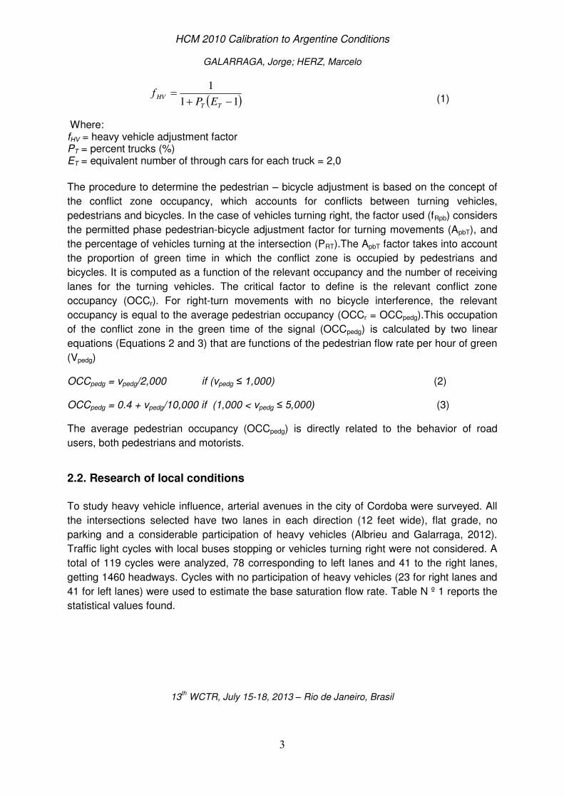
The procedure to determine the pedestrian – bicycle adjustment is based on the concept of

the conflict zone occupancy, which accounts for conflicts between turning vehicles,

pedestrians and bicycles. In the case of vehicles turning right, the factor used (fRpb) considers

the permitted phase pedestrian-bicycle adjustment factor for turning movements (ApbT), and

the percentage of vehicles turning at the intersection (PRT).The ApbT factor takes into account

the proportion of green time in which the conflict zone is occupied by pedestrians and

bicycles. It is computed as a function of the relevant occupancy and the number of receiving

lanes for the turning vehicles. The critical factor to define is the relevant conflict zone

occupancy (OCCr). For right-turn movements with no bicycle interference, the relevant

occupancy is equal to the average pedestrian occupancy (OCCr = OCCpedg).This occupation

of the conflict zone in the green time of the signal (OCCpedg) is calculated by two linear

equations (Equations 2 and 3) that are functions of the pedestrian flow rate per hour of green

(Vpedg)

OCCpedg = vpedg/2,000 if (vpedg ≤ 1,000) (2)

OCCpedg = 0.4 + vpedg/10,000 if (1,000 < vpedg ≤ 5,000) (3)

The average pedestrian occupancy (OCCpedg) is directly related to the behavior of road

users, both pedestrians and motorists.

2.2. Research of local conditions

To study heavy vehicle influence, arterial avenues in the city of Cordoba were surveyed. All

the intersections selected have two lanes in each direction (12 feet wide), flat grade, no

parking and a considerable participation of heavy vehicles (Albrieu and Galarraga, 2012).

Traffic light cycles with local buses stopping or vehicles turning right were not considered. A

total of 119 cycles were analyzed, 78 corresponding to left lanes and 41 to the right lanes,

getting 1460 headways. Cycles with no participation of heavy vehicles (23 for right lanes and

41 for left lanes) were used to estimate the base saturation flow rate. Table N º 1 reports the

statistical values found.




4

Table Nº1: Base Headway in seconds (s)

Lane Average Standard Dev. Minimum Maximum N° of cycles Right 2,029 0,209 1,6 2,33 23 Left 1,876 0,164 1,5 2,20 41 Both 1,931 0,195 1,5 2,33 64

The difference found between left and right lanes led to query whether these differences

were due to chance or not. Hypothesis test were conducted on equal variances in order to

determine the appropriate test for means. The F test for variances did not permit to reject the

hypothesis of equality, therefore it was applied a test of means with equal variances. Table

N° 2 shows the results of hypothesis tests performed.

Table Nº2: Hypothesis tests

Mean Headway (s) Variance (s2) F test for variances t test for means

Right lane 2,029 0,044 1,81410 1,99897

Left lane 1,876 0,027

Statistic 1,62878 3,23934

Ho No reject Reject

The higher headway found in the right lane (implies a lower saturation flow) can be related to

the lower speed due to regulations and lateral friction (generated by roadside activity).Taking

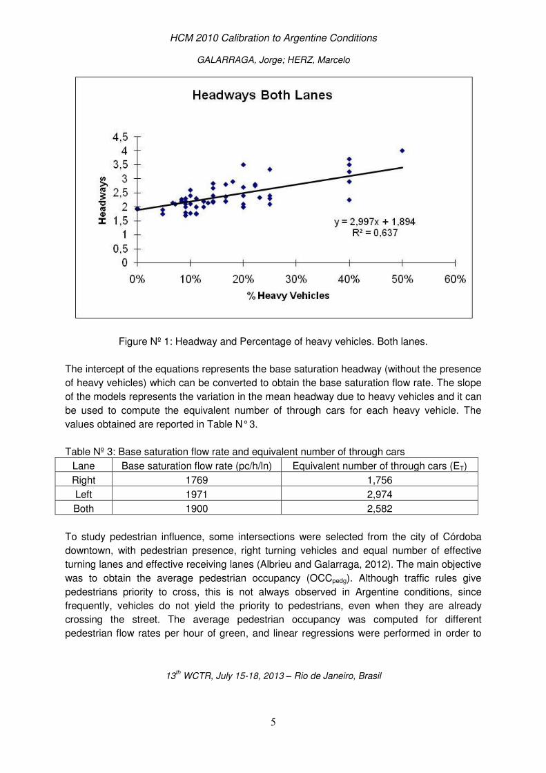
into account all 119 cycles, linear regression models were estimated, considering the mean

headway as dependent variable (Y) and the percentage of heavy vehicles as independent

variable (X). Regression results for the right and left lanes mean headways are shown in

Equations 4 and 5.

Right Lane Y= 1,583 X + 2,0346 (R2=0,41) (4)

Left Lane Y= 3,604 X + 1,8262 (R2=0,72) (5)

Figure N° 1 shows headways data and regression equation for both lanes.




5

Figure Nº 1: Headway and Percentage of heavy vehicles. Both lanes.

The intercept of the equations represents the base saturation headway (without the presence

of heavy vehicles) which can be converted to obtain the base saturation flow rate. The slope

of the models represents the variation in the mean headway due to heavy vehicles and it can

be used to compute the equivalent number of through cars for each heavy vehicle. The

values obtained are reported in Table N° 3.

Table Nº 3: Base saturation flow rate and equivalent number of through cars

Lane Base saturation flow rate (pc/h/ln) Equivalent number of through cars (ET)

Right 1769 1,756

Left 1971 2,974

Both 1900 2,582

To study pedestrian influence, some intersections were selected from the city of Córdoba

downtown, with pedestrian presence, right turning vehicles and equal number of effective

turning lanes and effective receiving lanes (Albrieu and Galarraga, 2012). The main objective

was to obtain the average pedestrian occupancy (OCCpedg). Although traffic rules give

pedestrians priority to cross, this is not always observed in Argentine conditions, since

frequently, vehicles do not yield the priority to pedestrians, even when they are already

crossing the street. The average pedestrian occupancy was computed for different

pedestrian flow rates per hour of green, and linear regressions were performed in order to




6

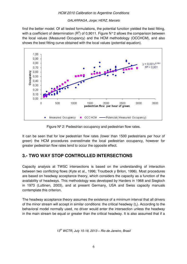
find the better model. Of all tested formulations, the potential function yielded the best fitting,

with a coefficient of determination (R2) of 0,9011. Figure N° 2 allows the comparison between

the local values (Measured Occupancy) and the HCM methodology (OCCHCM), and also

shows the best fitting curve obtained with the local values (potential equation).

Figure Nº 2: Pedestrian occupancy and pedestrian flow rates.

It can be seen that for low pedestrian flow rates (lower than 1500 pedestrians per hour of

green) the HCM procedures overestimate the local pedestrian occupancy, however for

greater pedestrian flow rates tend to occur the opposite effect.

3.- TWO WAY STOP CONTROLLED INTERSECTIONS

Capacity analysis at TWSC intersections is based on the understanding of interaction

between two conflicting flows (Kyte et al., 1996; Troutbeck y Brilon, 1996). Most procedures

are based on headway acceptance theory, which considers the capacity as a function of the

availability of headways. This methodology was developed by Harders in 1968 and Siegloch

in 1973 (Luttinen, 2003), and at present Germany, USA and Swiss capacity manuals

contemplate this criterion.

The headway acceptance theory assumes the existence of a minimum interval that all drivers

of the minor stream will accept in similar conditions: the critical headway (tc). According to the

behavioral model normally used, no driver would enter the intersection unless the headway

in the main stream be equal or greater than the critical headway. It is also assumed that if a




7

large enough headway is obtained, two or more drivers from the minor stream could use it.

The headway between them is called follow up time (tf).

3.1.- HCM 2010

HCM 2010 (TRB, 2010) analyzes TWSC intersections based on headway acceptance theory

and provides a detailed methodology to compute capacity and level of service for

intersections controlled by two stop signs (Chapter 19: TWSC)

HCM 2010 provides critical headways and follow up times corresponding to base conditions,

for different types of movements in TWSC intersections. Tables Nº 4 and Nº 5 show the

proposed values. In Table Nº 4 only critical headways in one stage are reported, for through

and left turn traffic from minor.

Table N° 4: Base Critical Headways from HCM2010, in seconds (s)

Vehicle

Movement Two lanes in major Four lanes in major Six lanes in major

Left turn from

major 4.1 4.1 5.3

U turn from

major NA

6.4 (wide lane)

6.9 (narrow lane)

5.6

Right turn from

minor 6.2 6.9 7.1

Through traffic

on minor 6.5 6.5 6.5

Left turn from

minor 7.1 7.5 6.4




8

Table N° 5: Base Follow up times base from HCM2010, in seconds (s)

Vehicle

Movement Two lanes in major Four lanes in major Six lanes in major

Left turn from

major 2.2 2.2 3.1

U turn from

major NA

2.5 (wide lane)

3.1 (narrow lane)

2.3

Right turn from

minor 3.3 3.3 3.9

Through traffic

on minor 4.0 4.0 4.0

Left turn from

minor 3.5 3.5 3.8

3.2.- Research of local conditions

In Argentina, intersections of a major avenue with a local street reproduce the conditions of a

TWSC intersection. Vehicles on the avenue have the priority and experiments no delay.

Vehicles on the minor street must wait until obtaining an adequate headway (Depiante y

Galarraga, 2012).

Local studies conducted at five intersections (Galarraga et al, 2002) showed that critical

headways and follow up times, computed by the maximum likelihood method, yielded lower

values than reported in the HCM2010. Local drivers clearly are more aggressive, therefore

capacity estimates may be higher but operation at the intersection may be less safe. The

90% confidence intervals of the mean critical headway and follow up time do not include

HCM2010 recommended values.

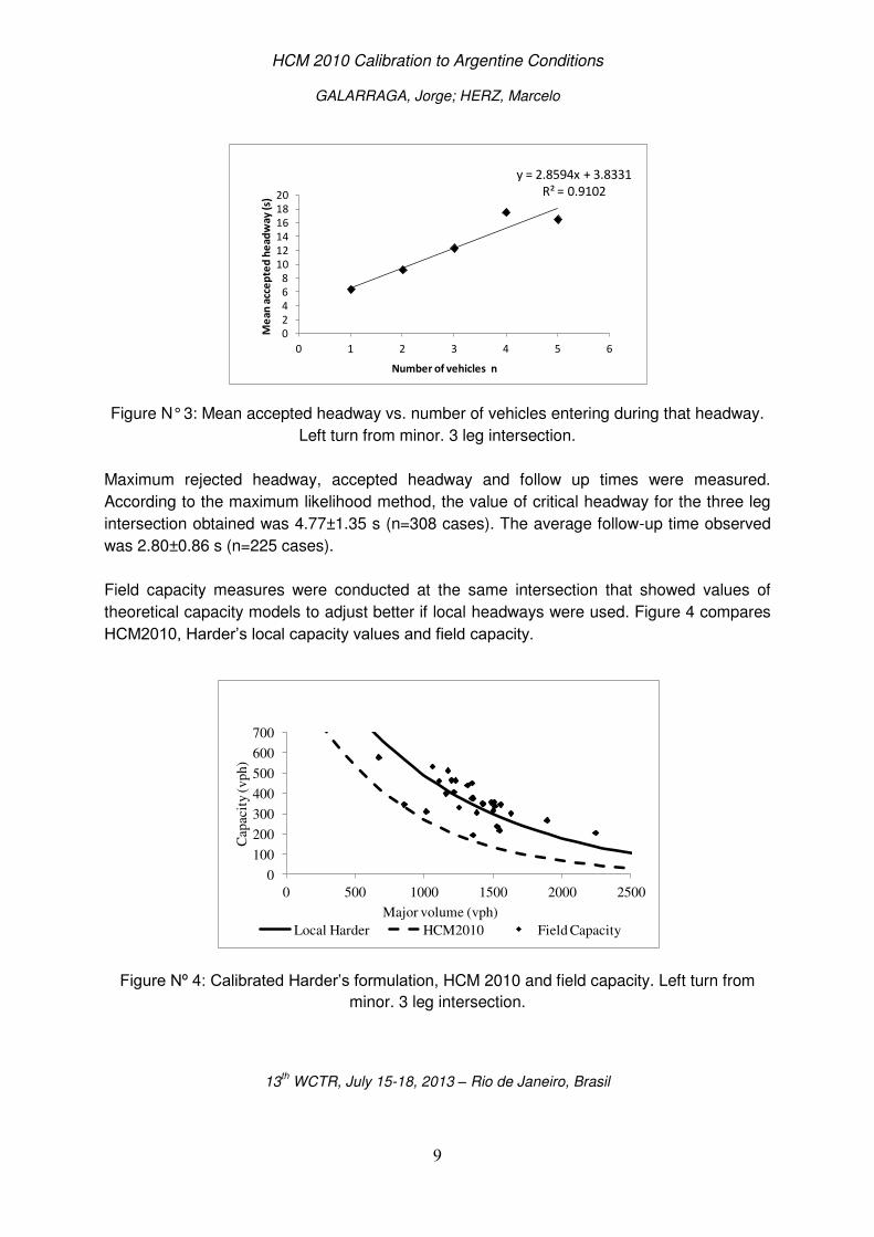
A local example of critical headway and follow up time estimation is showed in Figure Nº 3. In

this case the Siegloch method using linear regression model has been applied (Depiante,

2011). The results correspond to the left turn movement from the minor street. The slope of

the curve is the follow-up time (tf): 2.8594s. The critical headway (tc) can be obtained as the

intercept (3.8331s) plus half of the follow-up time (1.4297s): 5,2628s.




9

Figure N° 3: Mean accepted headway vs. number of vehicles entering during that headway.

Left turn from minor. 3 leg intersection.

Maximum rejected headway, accepted headway and follow up times were measured.

According to the maximum likelihood method, the value of critical headway for the three leg

intersection obtained was 4.77±1.35 s (n=308 cases). The average follow-up time observed

was 2.80±0.86 s (n=225 cases).

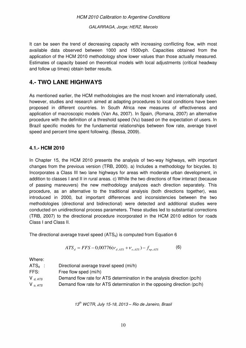
Field capacity measures were conducted at the same intersection that showed values of

theoretical capacity models to adjust better if local headways were used. Figure 4 compares

HCM2010, Harder’s local capacity values and field capacity.

Figure Nº 4: Calibrated Harder’s formulation, HCM 2010 and field capacity. Left turn from

minor. 3 leg intersection.

y = 2.8594x + 3.8331

R² = 0.9102

0

2

4

6

8

10

12

14

16

18

20

0 1 2 3 4 5 6

Me

an

acc

ep

ted

he

ad

wa

y (

s)

Number of vehicles n

0

100

200

300

400

500

600

700

0 500 1000 1500 2000 2500

Cap

acit

y (

vp

h)

Major volume (vph)

Local Harder HCM2010 Field Capacity




10

ATSnpATSoATSdd fFFSATS ,,, )(00776,0

It can be seen the trend of decreasing capacity with increasing conflicting flow, with most

available data observed between 1000 and 1500vph. Capacities obtained from the

application of the HCM 2010 methodology show lower values than those actually measured.

Estimates of capacity based on theoretical models with local adjustments (critical headway

and follow up times) obtain better results.

4.- TWO LANE HIGHWAYS

As mentioned earlier, the HCM methodologies are the most known and internationally used,

however, studies and research aimed at adapting procedures to local conditions have been

proposed in different countries. In South Africa new measures of effectiveness and

application of macroscopic models (Van As, 2007). In Spain, (Romana, 2007) an alternative

procedure with the definition of a threshold speed (Vu) based on the expectation of users. In

Brazil specific models for the fundamental relationships between flow rate, average travel

speed and percent time spent following. (Bessa, 2009).

4.1.- HCM 2010

In Chapter 15, the HCM 2010 presents the analysis of two-way highways, with important

changes from the previous version (TRB, 2000). a) Includes a methodology for bicycles. b)

Incorporates a Class III two lane highways for areas with moderate urban development, in

addition to classes I and II in rural areas. c) While the two directions of flow interact (because

of passing maneuvers) the new methodology analyzes each direction separately. This

procedure, as an alternative to the traditional analysis (both directions together), was

introduced in 2000, but important differences and inconsistencies between the two

methodologies (directional and bidirectional) were detected and additional studies were

conducted on unidirectional process parameters. These studies led to substantial corrections

(TRB, 2007) to the directional procedure incorporated in the HCM 2010 edition for roads

Class I and Class II.

The directional average travel speed (ATSd) is computed from Equation 6

(6)

Where:

ATSd : Directional average travel speed (mi/h)

FFS: Free flow sped (mi/h)

V d, ATS Demand flow rate for ATS determination in the analysis direction (pc/h)

V o, ATS Demand flow rate for ATS determination in the opposing direction (pc/h)




11

f np, ATS Adjustment factor for ATS determination for the percentage of no passing

zones in the analysis direction ( mi/h)

The adjustment factor f np, ATS is obtained from a table, as a function of the free flow speed,

the opposing demand flow rate and the percent of no passing zones. For greater opposing

demand flow rates the adjustment factor decreases. It should be noted that even for

segments with 0% of no passing zones, the adjustment factor is non zero, reflecting that it is

not independent of the other terms of the model.


Surveys were conducted in three road sections between 5 and 9 km in length located in the

Province of Córdoba. The locations were selected in rural areas, with high values of AADT

and known characteristics of traffic and topography (Maldonado et al, 2012). The main

objective was to calibrate the TSIS-CORSIM traffic simulation model (Mc Trans, 2010). All

the necessary traffic and geometry information for the HCM methodology and for the

simulation model was obtained from field surveys.

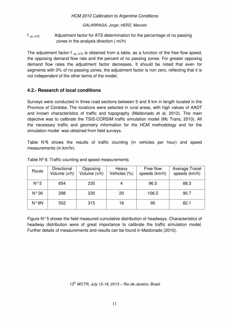
Table N°6 shows the results of traffic counting (in vehicles per hour) and speed

measurements (in km/hr).

Table Nº 6: Traffic counting and speed measurements

Route Directional

Volume (v/h) Opposing

Volume (v/h) Heavy

Vehicles (%) Free flow

speeds (km/h) Average Travel speeds (km/h)

N° 5 654 235 4 96.5 88.3

N° 36 298 230 20 106.5 90.7

N° 9N 552 315 18 95 82.1

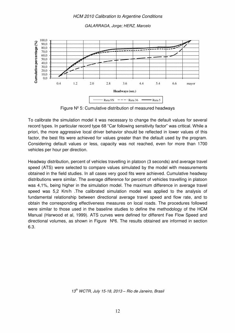
Figure N° 5 shows the field measured cumulative distribution of headways. Characteristics of

headway distribution were of great importance to calibrate the traffic simulation model.

Further details of measurements and results can be found in Maldonado (2010).




12

Figure Nº 5: Cumulative distribution of measured headways

To calibrate the simulation model it was necessary to change the default values for several

record types. In particular record type 68 “Car following sensitivity factor” was critical. While a priori, the more aggressive local driver behavior should be reflected in lower values of this

factor, the best fits were achieved for values greater than the default used by the program.

Considering default values or less, capacity was not reached, even for more than 1700

vehicles per hour per direction.

Headway distribution, percent of vehicles travelling in platoon (3 seconds) and average travel

speed (ATS) were selected to compare values simulated by the model with measurements

obtained in the field studies. In all cases very good fits were achieved. Cumulative headway

distributions were similar. The average difference for percent of vehicles travelling in platoon

was 4,1%, being higher in the simulation model. The maximum difference in average travel

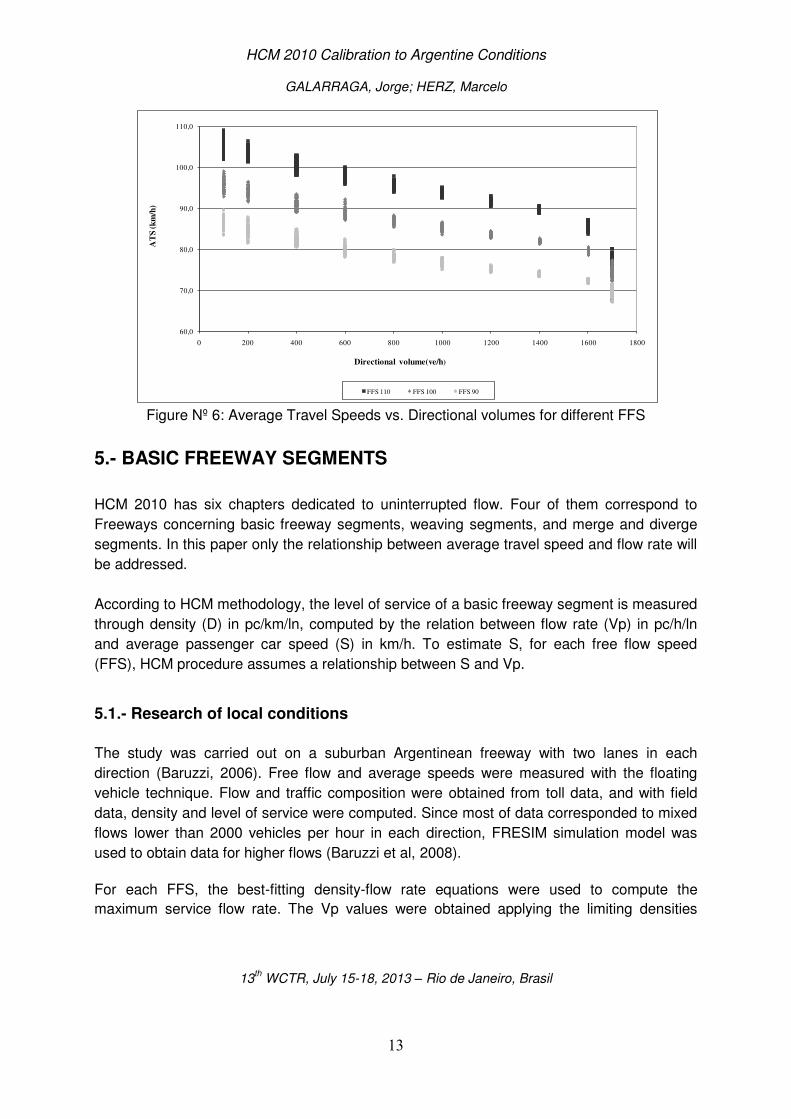
speed was 5,2 Km/h .The calibrated simulation model was applied to the analysis of

fundamental relationship between directional average travel speed and flow rate, and to

obtain the corresponding effectiveness measures on local roads. The procedures followed

were similar to those used in the baseline studies to define the methodology of the HCM

Manual (Harwood et al, 1999). ATS curves were defined for different Fee Flow Speed and

directional volumes, as shown in Figure Nº6. The results obtained are informed in section

6.3.

0,010,020,030,040,050,060,070,080,090,0

100,0

0.4 1.2 2.0 2.8 3.6 4.4 5.4 6.6 mayorCu

mu

lati

ve

pe

rce

nta

ge

(%

)

Headways (sec.)

Ruta 9N Ruta 36 Ruta 5




13

Figure Nº 6: Average Travel Speeds vs. Directional volumes for different FFS

5.- BASIC FREEWAY SEGMENTS

HCM 2010 has six chapters dedicated to uninterrupted flow. Four of them correspond to

Freeways concerning basic freeway segments, weaving segments, and merge and diverge

segments. In this paper only the relationship between average travel speed and flow rate will

be addressed.

According to HCM methodology, the level of service of a basic freeway segment is measured

through density (D) in pc/km/ln, computed by the relation between flow rate (Vp) in pc/h/ln

and average passenger car speed (S) in km/h. To estimate S, for each free flow speed

(FFS), HCM procedure assumes a relationship between S and Vp.


The study was carried out on a suburban Argentinean freeway with two lanes in each

direction (Baruzzi, 2006). Free flow and average speeds were measured with the floating

vehicle technique. Flow and traffic composition were obtained from toll data, and with field

data, density and level of service were computed. Since most of data corresponded to mixed

flows lower than 2000 vehicles per hour in each direction, FRESIM simulation model was

used to obtain data for higher flows (Baruzzi et al, 2008).

For each FFS, the best-fitting density-flow rate equations were used to compute the

maximum service flow rate. The Vp values were obtained applying the limiting densities

60,0

70,0

80,0

90,0

100,0

110,0

0 200 400 600 800 1000 1200 1400 1600 1800

AT

S (

km

/h)

Directional volume(ve/h)

FFS 110 FFS 100 FFS 90




14

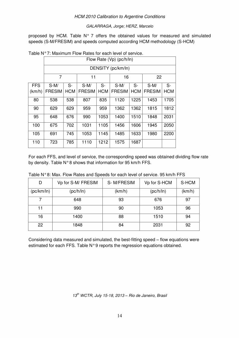
proposed by HCM. Table N° 7 offers the obtained values for measured and simulated

speeds (S-M/FRESIM) and speeds computed according HCM methodology (S-HCM)

Table N° 7: Maximum Flow Rates for each level of service.

Flow Rate (Vp) (pc/h/ln)

DENSITY (pc/km/ln)

7 11 16 22

FFS

(km/h)

S-M/

FRESIM

S-

HCM

S-M/

FRESIM

S-

HCM

S-M/

FRESIM

S-

HCM

S-M/

FRESIM

S-

HCM

80 538 538 807 835 1120 1225 1453 1705

90 629 629 959 959 1362 1362 1815 1812

95 648 676 990 1053 1400 1510 1848 2031

100 675 702 1031 1105 1456 1606 1945 2050

105 691 745 1053 1145 1485 1633 1980 2200

110 723 785 1110 1212 1575 1687

For each FFS, and level of service, the corresponding speed was obtained dividing flow rate

by density. Table N° 8 shows that information for 95 km/h FFS.

Table N° 8: Max. Flow Rates and Speeds for each level of service. 95 km/h FFS

D Vp for S-M/ FRESIM S- M/FRESIM Vp for S-HCM S-HCM

(pc/km/ln) (pc/h/ln) (km/h) (pc/h/ln) (km/h)

7 648 93 676 97

11 990 90 1053 96

16 1400 88 1510 94

22 1848 84 2031 92

Considering data measured and simulated, the best-fitting speed – flow equations were

estimated for each FFS. Table N° 9 reports the regression equations obtained.




15

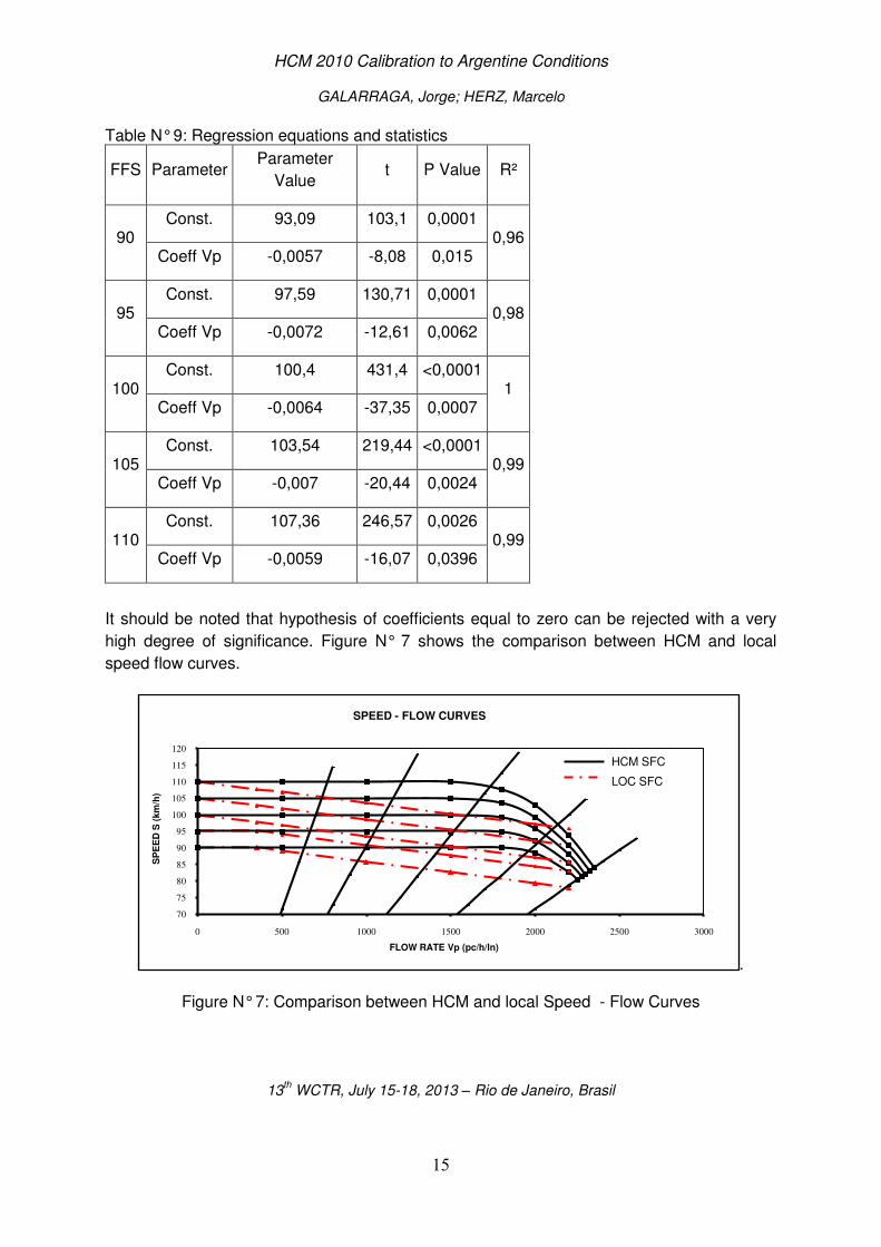
Table N° 9: Regression equations and statistics

FFS Parameter Parameter

Value t P Value R²

90 Const. 93,09 103,1 0,0001

0,96 Coeff Vp -0,0057 -8,08 0,015

95 Const. 97,59 130,71 0,0001

0,98 Coeff Vp -0,0072 -12,61 0,0062

100 Const. 100,4 431,4 <0,0001

1 Coeff Vp -0,0064 -37,35 0,0007

105 Const. 103,54 219,44 <0,0001

0,99 Coeff Vp -0,007 -20,44 0,0024

110 Const. 107,36 246,57 0,0026

0,99 Coeff Vp -0,0059 -16,07 0,0396

It should be noted that hypothesis of coefficients equal to zero can be rejected with a very

high degree of significance. Figure N° 7 shows the comparison between HCM and local

speed flow curves.

.

Figure N° 7: Comparison between HCM and local Speed - Flow Curves

70

75

80

85

90

95

100

105

110

115

120

0 500 1000 1500 2000 2500 3000

SP

EE

D S

(km

/h)

FLOW RATE Vp (pc/h/ln)

SPEED - FLOW CURVES

HCM SFC

LOC SFC




16

6.- RECOMMENDATIONS

6.1.- Signalized Intersections

For adjustment factor of Heavy Vehicles: The equivalent number of through cars obtained for

local conditions (ET = 2,5) is recommended to apply on lanes with presence of trucks. For

lanes with only buses is recommended to apply the equivalent number of through cars

proposed by the HCM (ET = 2,0)

For adjustment factor of Pedestrians: It has been observed that, for flow rates below 1500

pedestrians per hours of green, the average pedestrian occupancy (OCCpedg) in local

conditions is lower than the values proposed by the HCM. For greater flows the pedestrian

activity is enough high at the intersection that drivers tend to respect priorities and therefore

the average pedestrian occupancy for local conditions is similar to the values recommended

by the HCM. In order to better represent local reality is advisable to use, for flows lower than

1500 pedestrians per hour of green, Equation 7 for the calculation of the average pedestrian

occupancy (OCCpedg)

(7)

6.2.- Two Way Stop Controlled Intersections

Local values for critical headways and follow up times are proposed. Table Nº 10 shows the

corresponding headways for local and HCM conditions.

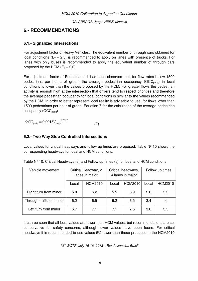
Table N° 10: Critical Headways (s) and Follow up times (s) for local and HCM conditions

Vehicle movement Critical Headway, 2

lanes in major

Critical headways,

4 lanes in major

Follow up times

Local HCM2010 Local HCM2010 Local HCM2010

Right turn from minor 5.0 6.2 5.5 6.9 2.6 3.3

Through traffic on minor 6.2 6.5 6.2 6.5 3.4 4

Left turn from minor 6.7 7.1 7.1 7.5 3.0 3.5

It can be seen that all local values are lower than HCM values, but recommendations are set

conservative for safety concerns, although lower values have been found. For critical

headways it is recommended to use values 5% lower than those proposed in the HCM2010

7617.00018.0 pedgpedg VOCC




17

for through and left turning movements and values 20% lower in the case of right turns. For

follow-up times it is recommended to use values 15% lower than those proposed in the

HCM2010 for through and left turning movements and values 20% lower for the case of right

turns.

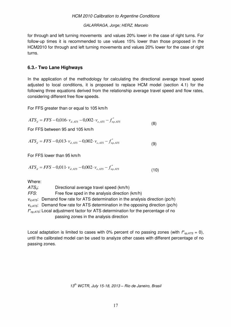
6.3.- Two Lane Highways

In the application of the methodology for calculating the directional average travel speed

adjusted to local conditions, it is proposed to replace HCM model (section 4.1) for the

following three equations derived from the relationship average travel speed and flow rates,

considering different free flow speeds.

For FFS greater than or equal to 105 km/h

(8)

For FFS between 95 and 105 km/h

(9)

For FFS lower than 95 km/h

(10)

Where:

ATSd: Directional average travel speed (km/h)

FFS: Free flow sped in the analysis direction (km/h)

vd,ATS: Demand flow rate for ATS determination in the analysis direction (pc/h)

vo,ATS: Demand flow rate for ATS determination in the opposing direction (pc/h)

f*np,ATS: Local adjustment factor for ATS determination for the percentage of no

passing zones in the analysis direction

Local adaptation is limited to cases with 0% percent of no passing zones (with f*np,ATS = 0),

until the calibrated model can be used to analyze other cases with different percentage of no

passing zones.

*

,,, 002,0016,0 ATSnpATSoATSdd fvvFFSATS

*


*





18

6.4.- Basic Freeway Segments

Considering the results obtained, adopting an average coefficient for Vp, equation 11 is

proposed for local conditions

S = FFS – 0,0064 Vp. (11)

In the analyzed freeway the measured and simulated average speed values (S) decrease

faster than predicted with the HCM methodology. In the case of FFS lower than 95 km/h, S

begins to decrease around 300 pc/h/ln, and for FFS greater than 100 km/h, S begins to

decrease at even lower flow values. In the curves obtained using the HCM procedures S

begins to decrease above 1300 pc/h/ln (or greater with lower FFS), becoming closer to the

measured and simulated values near congestion. (see Figure Nº 7).

According to the performed analysis, it is concluded that for suburban freeways with two

lanes in each direction, considering local driver and vehicle characteristics, average travel

speeds decrease around 1 km/h for every flow rate increase of 150 pc/h/ln. This fact may be

explained by the high coefficients of variation in operating speeds. The high standard

deviations are produced by the heterogeneity of the vehicle fleet (old and new cars) and by

the unconstrained driver behavior (without speed limit enforcement).

6.5 Further research

Continuously increase of motorization and society demands for mobility and sustainable

transportation, require better understanding of local traffic characteristics, as influenced by

drivers behavior and vehicle fleet. The HCM methodologies have proven to be useful when

calibrated to adjust to Argentinean conditions.

ACKNOWLEDGEMENTS

The authors thank the Secretary of Science and Technology of the Universidad Nacional de

Cordoba (Secyt-UNC) for the research financial support received.

The authors acknowledge the contribution of Maria Laura Albrieu, Violeta Depiante, Marcelo

Maldonado, Alejandro Baruzzi, and other research collaborators at the National University of

Cordoba.




19

REFERENCES

Albrieu L., Galarraga J. (2012). Recomendaciones para la aplicación de la metodología del

HCM para intersecciones semaforizadas en Argentina. XVI Congreso Argentino de

Vialidad y Tránsito. Córdoba. Argentina.

Akcelik & Assoc. (2002) AaSIDRA User Guide. Akcelik & Associates Pty Ltd. Melbourne.

Australia

Baruzzi, A. (2006) “Recomendaciones para la aplicación de la metodología del HCM 2000 en autopistas argentinas” Tesis de Maestría en Ciencias de la Ingeniería Mención en Transporte. Facultad de Ciencias Exactas, Físicas y Naturales, Universidad Nacional

de Córdoba, Argentina.

Baruzzi, A; Galarraga J., Herz, M. (2008). Speed Flow Curves in Argentinean Freeways.

Proceedings of 6th Internacional Conference on Traffic and Transportation Studies.

Beijing Jiatong University. China.

Bessa Júnior, J.E., (2009). “Caracterizacao do fluxo do tráfego em rodovias de pista simples do Estado de Sao Paulo” Disertación para obtener titulo de Maestría. Escuela de

Ingeniería de San Carlos, San Pablo

Depiante, V. (2011) Giros a la izquierda en intersecciones no semaforizadas. Tesis de

Maestría en Ciencias de la Ingeniería–Mención Transporte-. Facultad de Ciencias

Exactas, Físicas y Naturales, Universidad Nacional de Córdoba. Argentina.

Depiante V., Galarraga J. (2012): Recomendaciones para la aplicación de la metodología del

HCM para intersecciones no semaforizadas en Argentina. XVI Congreso Argentino

de Vialidad y Tránsito. Córdoba. Argentina.

Galarraga, J., Herz M., Depiante V., Ruiz Juri N. (2002) - Intervalos críticos: comportamiento

de los conductores y su impacto en la eficiencia y seguridad de las intersecciones no

semaforizadas. Diferencias locales con respecto a estudios del HCM 2000. Congreso

Provsegur.

Harwood, D., May A.D., Anderson I.B., Leiman L., Archilla, R. (1999) “Capacity And Quality Of Service Of Two-Lane Highways” National Cooperative Highway Research Program Report 3-55(3). Transportation Research Board National Research Council

Midwest Research Institute University of California-Berkeley USA. November 1999.

Kyte, M., Z. Tian, Z. Mir, Z. Hameedmansoor, W. Kittelson, M. Vandehey, B. Robinson, W.

Brilon, L. Bondzio, N. Wu, R. Troutbeck, (1996) Capacity and Level of Service at

Unsignalized Intersections. Final Report: Volume 1 – Two Way Stop-Controlled

Intersections. National Cooperative Highway Research Program 3-46.




20

Luttinen, T. (2003) Capacity at Unsignalized Intersections. TL Consulting Engineers, Ltd.

Lahti . TL Research Report No 3. ISBN 952-5415-02-3, ISSN 1458-3313.

Luttinen, T. (2006) Capacity and Level-of-Service Estimation in Finland. Fifth International

Symposium on Highway Capacity and Quality of Service - Yokohama, Japan.

Maldonado M., Herz M., Galarraga J. (2012): Aplicación de la metodología del HCM 2010

adaptada a carreteras argentinas. XXVI Congreso Argentino de Vialidad y Tránsito.

Córdoba. Argentina.

Maldonado, M. (2010) “Validación de la Metodología del Manual de Capacidad HCM a las condiciones locales para el Análisis de Operación en Carreteras” Tesis de Maestría

en Ciencias de la Ingeniería Mención en Transporte. Facultad de Ciencias Exactas,

Físicas y Naturales, Universidad Nacional de Córdoba, Argentina

McTrans Center (2010) TSIS-CORSIM Release 6.2 University of Florida, USA.

Romana, M. G. (2007), “La Definición de un umbral de velocidad para medir el nivel de

servicio en carreteras de dos carriles” Revista Rutas España, Agosto 2007.

Teply S., Allingham D.I., Richarson D. B., Stephenson, D.B. (2006). Canadian Capacity

Guide for Signalized Intersection. Institute of Transportation Engineers. District 7

Canada. Editor J. W. Gough. 3th Edition

TRB (2000) Highway Capacity Manual. Transportation Research Board, National Research

Council, Washington, D.C., USA.

TRB (2007) Committee AHB40, Highway Capacity and Quality of Service “Approved Corrections and Changes for the HCM 2000. Update 2007”. Transportation Research Board National Research Council, Washington, D.C., USA.

TRB (2010) Highway Capacity Manual. Transportation Research Board, National Research

Council, Washington, D.C., USA.

Troutbeck, R.; W. Brilon (1996) Unsignalized Intersection Theory. Chapter 8. Página de

internet: http://www.tfhrc.gov/its/tft/chap8.pdf.

Van As, C. (2007). South African Highway Capacity Research. TRB Workshop Presentation.

South African National Roads Agency, Limited, 2007.

http://www.tfhrc.gov/its/tft/chap8.pdf

Documents

hcm 2010 calibration to argentine conditions