Height fluctuations of stationary TASEP on a ring in relaxation

time scale

Zhipeng Liu∗

October 14, 2016

Abstract

We consider the totally asymmetric simple exclusion process on a ring with stationary initial condi-

tions. The crossover between KPZ dynamics and equilibrium dynamics occurs when time is proportional

to the 3/2 power of the ring size. We obtain the limit of height function along the direction of charac-

teristic line in this time scale. The two-point covariance function in this scale is also discussed.

1 Introduction

In this paper we consider the totally asymmetric simple exclusion process (TASEP) on a ring of size L which

we denote by ZL. The dynamics of TASEP on the ring is the same as that of TASEP on Z except the

particle at the site L− 1, once it jumps, moves to the site 0 if 0 is empty, here the i denotes the element i

(mod L) in ZL for i ∈ {0, 1, · · · , L− 1}. Let ηi = ηi(t) the occupation variable of this model, 0 ≤ i ≤ L− 1.

ηi is 1 if the site i is occupied or 0 if the site i is empty. We extend the occupation variable to Z periodically

by defining ηi(t) = ηi+L(t) for all i ∈ Z. Define the following height function

ht(`) =

2J0(t) +

∑`j=1(1− 2ηj(t)), ` ≥ 1,

2J0(t), ` = 0,

2J0(t)−∑0j=`+1(1− 2ηj(t)), ` ≤ −1,

(1.1)

where J0(t) counts the number of particles jumping through the bond from 0 to 1 on ZL during the time

interval [0, t]. Note that ht(`)− h0(`) = 2J`(t), where J`(t) counts the number of particles jumping through

the bond from ` (mod L) to ` + 1 (mod L) on ZL during the time interval [0, t]. Although η`(t), J`(t) are

both periodic in `, ht(`) is not periodic except when the system is half-filled. Indeed, we have ht(` + L) =

ht(`) + (L− 2N) for all ` ∈ Z and t ≥ 0, where N =∑L−1j=0 ηj is the number of particles on the ring.

We are interested in the fluctuations of ht(`) when t and ` both increase of order O(L3/2), and L,N go

to infinity proportionally. The scale t = O(L3/2) is called the relaxation time scale, which was first studied

by Gwa and Spohn [10]. At this relaxation time scale, one expects to see a crossover between the KPZ

dynamics and the Gaussian dynamics and hence the fluctuations are of great interest to both math and

physics communities. The crossover limiting distributions were obtained only recently by Prolhac [15] and

Baik and Liu [4]. In [15], Prolhac obtained (not rigorously) the limit of the current fluctuations for step, flat

and stationary initial conditions in the half particle system (with the restriction L = 2N). Independently,

Baik and Liu also obtained the limit in a more general setting of N and L for flat and step initial conditions

∗Courant Institute of Mathematical Sciences, New York University, New York, NY 10012

email: zhipeng@cims.nyu.edu

1

in [4]1. The main goal of this paper is to extend the work of [4] to the stationary initial condition and

prove the rigorous limit theorem of ht(`) in relaxation time scale. Compared to [15], there are some other

differences except for the rigorousness: We consider a more general setting of stationary initial conditions

than [15], and more generally the height function ht(`), than the current in [15], which is equivalent to ht(0).

Hence the limiting distribution obtained in this paper, FU (x; τ, γ) in Theorem 1.1, contains two parameters

of time τ and location γ, in contrast to that of only time parameter in [15].

Due to the ring structure, the number of particles is invariant and hence it is natural to consider the

following uniform initial condition of N particles: initially all possible configurations of N particles on the

ring of size L are of equal probability, i.e.,(LN

)−1= N !(L−N)!

L! . This initial condition is stationary, and is the

unique one for fixed number of particles N and ring size L [12].

For this uniform initial condition, there is a characteristic line ` = (1−2ρ)t in the space-time plane, here

ρ = NL−1 is the density of the system. The main theorem of this paper is on the fluctuations of h`(t) near

the characteristic line in relaxation time scale.

Theorem 1.1. Let c1 and c2 be two fixed constants satisfying 0 < c1 < c2 < 1. Suppose NL is a sequence

of integers such that c1L ≤ NL ≤ c2L for all L. We consider the TASEP on a ring of size L with NLparticles. Assume that they satisfy the uniform initial condition. Denote ρL = NL/L. Let τ and w be two

fixed constants satisfying τ > 0 and w ∈ R. Suppose

tL =τ√

ρL(1− ρL)L3/2. (1.2)

Then along the line

`L = (1− 2ρL)tL + 2w(ρL(1− ρL))1/3t2/3L , (1.3)

we have

limL→∞

P

(htL(`L)− (1− 2ρL)`L − 2ρL(1− ρL)tL

−2ρ2/3L (1− ρL)2/3t

1/3L

≤ x

)= FU (τ1/3x; τ, 2wτ2/3) (1.4)

for each x ∈ R. Here FU (x; τ, γ) is a distribution function defined in (2.1) for any τ > 0 and γ = 2wτ2/3 ∈ R.

It satisfies FU (x; τ, γ) = FU (x; τ, γ + 1) and FU (x; τ, γ) = FU (x; τ,−γ).

Remark 1.1. In [15], Prolhac obtained (1.4) when `N = 0 and ρL = 1/2 (and hence w = 0, γ = 0) with a

different formula of the limiting distribution. His proof, as mentioned before, is not completely rigorous.

Note that if we write γ = 2wτ2/3, then the line (1.3) can be rewritten as

`L = (1− 2ρL)tL + γL. (1.5)

This expression gives an intuitive reason why the limiting function FU (x; τ, γ) is periodic on γ: It is the

periodicity of the shifted height function htL(`L + L)− (1− 2ρL)(`L + L) = htL(`L)− (1− 2ρL)`L.

To better understand the parametrization in the above theorem, we compare it with the infinite TASEP

with stationary condition, i.e., the stationary TASEP on Z. Suppose initially each site in Z is occupied

independently with probability p. Then the height fluctuation converges along the line ` = (1 − 2p)t +

2w(p(1− p))1/3t2/3 for any given constant w ∈ R, see [9, 2],

limt→∞

P(ht(`)− (1− 2p)`− 2p(1− p)t−2p2/3(1− p)2/3t1/3

≤ x)

= Fw(x), x ∈ R, (1.6)

1The formulas of the limiting distribution in two papers [15] and [4] are slightly different and it is yet to be proved that they

are indeed the same. The numeric plots show that they do agree.

2

where Fw(s) is the Baik-Rains distribution defined in [6]2. Theorem 1.1 of this paper shows that for the

stationary TASEP on a ring with uniform initial condition in relaxation time scale, similar limiting laws hold

near the characteristic line. The difference is that for the ring TASEP, the fluctuations have a periodicity

on the parameter γ = 2wτ2/3, which is not present in the infinite TASEP model.

The leading terms (1−2ρL)`L and 2ρL(1−ρL)tL in htL(`L) can be explained as following. The first term

(1− 2ρL)`L measures the change of height along the direction `L: For fixed tL, recall that htL(`L)− htL(0)

grows as (1− 2ρL)`L in the leading order and satisfies htL(`L +L) = htL(`L) + (1− 2ρL)L. The second term

2ρL(1 − ρL)tL measures the time-integrated current at a fixed location: htL(`L) − h0(`L) = 2J0(tL) which

grows as 2ρL(1− ρL)tL in the leading order.

As an application of Theorem 1.1, we can express the limit of two-point covariance function in terms

of FU (x; τ, γ). Recall the occupation variable η`(t) at the beginning of the paper. Define the two-point

covariance function

S(`; t) := E (η`(t)η0(0))− ρ2 (1.7)

where ρ = N/L is the system density. It is known that for the stationary TASEP, there is a relation between

this two-point function S(`; t) and the height function h`(t): 8S(`; t) = Var(ht(` + 1)) − 2Var(ht(`)) +

Var(ht(`−1)). This relation was proved for the infinite TASEP in [14] but the proof is also valid for TASEP

on a ring after minor modifications. Using this identity and the tail estimate which is provided in the

appendix A, we obtain the following result. The proof is almost the same as that for the stationary TASEP

on Z, see [3], and hence we omit it.

Corollary 1.1. Suppose NL, tL and `L are defined as in Theorem 1.1 with the same constants τ > 0 and

γ = 2wτ2/3 ∈ R. Then we have

limL→∞

2t2/3L S(`L, tL)

ρ2/3L (1− ρL)2/3

= g′′U (γ; τ), (1.8)

if integrated over smooth functions in γ with compact support, where

gU (γ; τ) := τ2/3

∫Rx2dFU (x; τ, γ). (1.9)

Another application is that one can obtain the height fluctuations for other stationary TASEP on a ring.

Note that the uniform initial conditions with N = 0, 1, · · · , L form a complete basis for all stationary initial

conditions. Hence we may apply Theorem 1.1 for other stationary initial conditions. One example is the

Bernoulli condition. Suppose initially each site of the ring is occupied independently with probability p,

where p is a constant satisfies 0 < p < 1. Then we have the following result.

Corollary 1.2. Suppose p ∈ (0, 1) is a fixed constant. We consider the TASEP on the ring of size L with

Bernoulli initial condition of parameter p. Suppose w ∈ R, τ > 0 and x ∈ R are fixed constants. Denote

tL =τ√

p(1− p)L3/2,

`L = (1− 2p)tL + 2w(p(1− p))1/3t2/3L ,

(1.10)

Then

limL→∞

P

(htL(`L)− (1− 2p)`L − 2p(1− p)tL

−2p2/3(1− p)2/3t1/3L

≤ x

)= FB(τ1/3x; τ, 2wτ2/3). (1.11)

2In [6], Fw(s) was denoted by H(s+ w2;w/2,−w/2).

3

Here FB(x; τ, γ) is a distribution function for arbitrary τ > 0 and γ = 2wτ2/3 ∈ R, given by

FB(x; τ, γ) :=1

2√

2πτ

∫Re−

(y−γ)2

8τ2 FU

(x+

γ2 − y2

4τ; τ, y

)dy. (1.12)

A formal proof is as following. Assume there are pL + y√p(1− p)L1/2 particles initially. By applying

Theorem 1.1, we obtain that

P

(htL(`L)− (1− 2p)`L − 2p(1− p)tL

−2p2/3(1− p)2/3t1/3L

≤ x

∣∣∣∣∣ pL+ y√p(1− p)L1/2 particles with uniform initial condition

)(1.13)

converges to

FU

(τ1/3x− γy − τy2; τ, γ + 2yτ

)(1.14)

as L→∞, where γ = 2wτ2/3. Together with the central limit theorem, we obtain

limL→∞

(htL(`L)− (1− 2p)`L − 2p(1− p)tL

−2p2/3(1− p)2/3t1/3L

≤ x

)=

1√2π

∫Re−y

2/2FU

(τ1/3x− γy − τy2; τ, γ + 2yτ

)dy.

(1.15)

By a simple change of variables we arrive at (1.12). This argument can be made rigorous by a simple tail

estimate on the number of particles and then by the dominated convergence theorem. Since the argument

is standard, we omit the details.

Recall that FU (x; τ, γ) is symmetric on γ. Hence by using the formula (1.12) we have FB(x; τ, γ) =

FB(x; τ,−γ). However, different from FU (x; τ, γ), we do not expect FB(x; τ, γ) = FB(x; τ, γ + 1). It is

because by definition ht(` + L) − ht(`) − (1 − 2p)L = −2∑`+Lj=`+1(ηj(t) − p) ≈ −2L1/2

√p(1− p)χ where χ

is a standard Gaussian random variable. Hence formally

htL(`L + L)− (1− 2p)(`L + L)− 2p(1− p)tL−2p2/3(1− p)2/3t

1/3L

≈ htL(`L)− (1− 2p)`L − 2p(1− p)tL−2p2/3(1− p)2/3t

1/3L

+χ

τ1/3. (1.16)

Here the two random variables on the right hand side of (1.16) are not necessarily independent. This relation

still strongly indicates that FB(τ1/3x; τ, γ + 1) is not the same as FB(τ1/3x; τ, γ).

The organization of this paper is as following. In Section 2 we give the explicit formula and some

properties of FU (x; τ, γ). The proof of Theorem 1.1 is given in Section 3 and 4: The finite time distribution

formula is provided in Section 3 and then the asymptotics in Section 4. Finally in the appendix A we give

some tail bounds related to the distribution function FU (x; τ, γ).

Acknowledgement

The author would like to thank Jinho Baik, Ivan Corwin and Peter Nejjar for useful discussions.

2 Limiting distribution FU

The limiting distribution FU (x; τ, γ) is defined as following

FU (x; τ, γ) = −∮

d

dx

(exA1(z)+τA2(z)+2B(z) det

(I −K(2)

z;x

)) dz√2πiz2

(2.1)

4

where the integral is over an arbitrary simple closed contour within the disk |z| < 1 and with 0 inside. The

terms Ai(z) are given by

A1(z) = − 1√2π

Li3/2(z), A2(z) = − 1√2π

Li5/2(z), (2.2)

and B(z) is given by

B(z) =1

4π

∫ z

0

(Li1/2(y))2

ydy. (2.3)

Here Lis(z) is the polylogarithm function defined by Lis(z) :=∑∞k=1

zk

ks for all |z| < 1, and then to be

analytical continuous to the complex plane except the half line R≥1. And log is the usual logarithm function

with branch cut R≤0. The operator K(2)z;x is defined on the set Sz,left = {ξ : e−ξ

2/2 = z,Re(ξ) < 0} with

kernel

K(2)z;x(ξ1, ξ2) = K(2)

z;x(ξ1, ξ2; τ, γ) =∑

η∈Sz,left

eΦz(ξ1;x,τ)+Φz(η;x,τ)+ γ2 (ξ21−η

2)

ξ1η(ξ1 + η)(η + ξ2), (2.4)

where

Φz(ξ;x, τ) = −1

3τξ3 + xξ −

√2

π

∫ ξ

−∞Li1/2(e−ω

2/2)dω, ξ ∈ Sz,left. (2.5)

The terms Ai(z), B(z) and K(2)z;x are defined in [4]. They appeared in the limiting distributions of TASEP

on a ring with step initial condition in relaxation time scale, more explicitly in the distribution function

F2(x; τ, γ) as shown below

F2(x; τ, γ) =

∮exA1(z)+τA2(z)+2B(z) det

(I −K(2)

z;x

) dz

2πiz, (2.6)

see (4.10) of [4]. It is known that they are well defined and bounded uniformly on the choice of z (but the

bound may depend on the contour). Furthermore, the Fredholm determinant det(I −K(2)

z;x

)is periodic and

symmetric on γ, which implies F2(x; τ, γ) = F2(x; τ, γ + 1) and F2(x; τ, γ) = F2(x; τ,−γ).

To ensure FU (x; τ, γ) in (2.1) is well defined, we still need to check that the derivative in the integrand

exists and is uniformly bounded. The only non-trivial part is to check ddx det

(I −K(2)

z;x

). This can be proved

by directly using the super-exponential decaying property of the kernel. The argument is standard and we

do not provide details. Alternately, our analysis in Section 4.6 also implies ddx det

(I −K(2)

z;x

)is a limit of a

uniformly bounded sequence hence it is also uniformly bounded. See Lemma 4.5 and 4.6.

As we discussed in Remark 1.1, the limiting distribution when γ = 0 was obtained in [15]. Numeric plots

of our formula FU (x; τ, 0) match the limiting distribution obtained in [15] well, see Figure 1 in this paper

and Fig.5.b in [15]. However, a rigorous proof of the equivalence on FU (x; τ, 0) and their formula (see (10)

of [15]) is still missing.

For any fixed τ > 0 and γ ∈ R, the function FU (x; τ, γ) is a distribution function. The proof is not

trivial and we prove it in the appendix A. Similar to F2(x; τ, γ), the function FU (x; τ, γ) has the properties

FU (x; τ, γ+ 1) = FU (x; τ, γ) and FU (x; τ, γ) = FU (x; τ,−γ). Also by using the following simple identity (see

(11) of [8])

E(htL(`L)) = (1− 2ρL)`L + 2ρL(1− ρL)tL +2ρL(1− ρL)tL

L− 1(2.7)

which can also be checked directly from the definition, we formally have∫RxdFU (x; τ, γ) = −τ. (2.8)

5

-4 -3 -2 -1 0 1 2 3 4

0

0.05

0.1

0.15

0.2

0.25

0.3

0.35

0.4

0.45

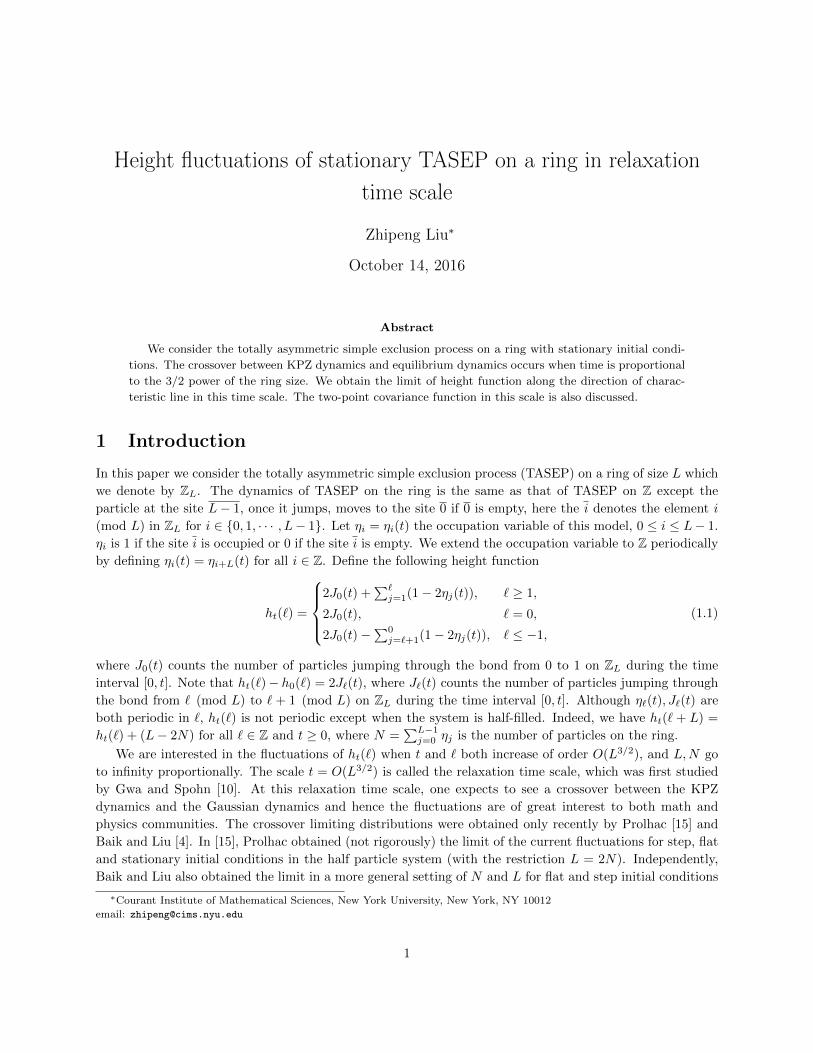
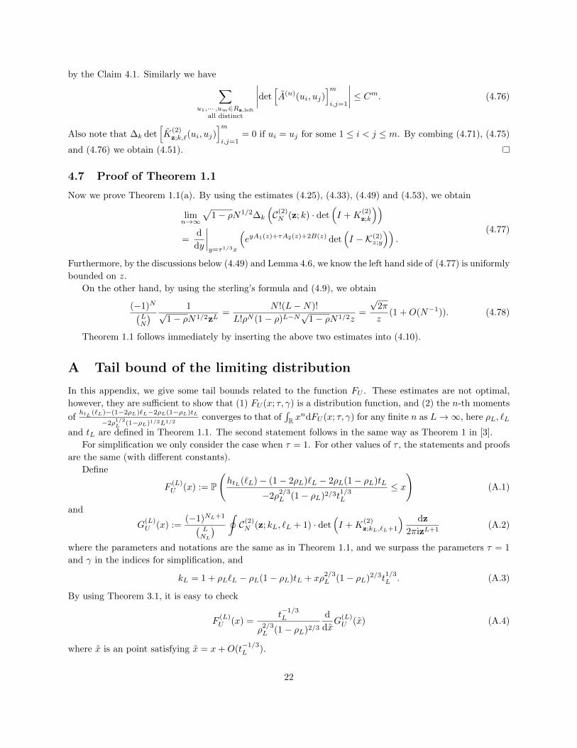
Figure 1: The three dashed lines are, from left to

right, density functions of FU (τ1/3x; τ, 0) with τ = 1,

0.1, and 0.02 respectively. And the solid line is the

density function of Baik-Rains distribution F0(x).

-6 -4 -2 0 2 4 6

0

0.05

0.1

0.15

0.2

0.25

0.3

0.35

0.4

0.45

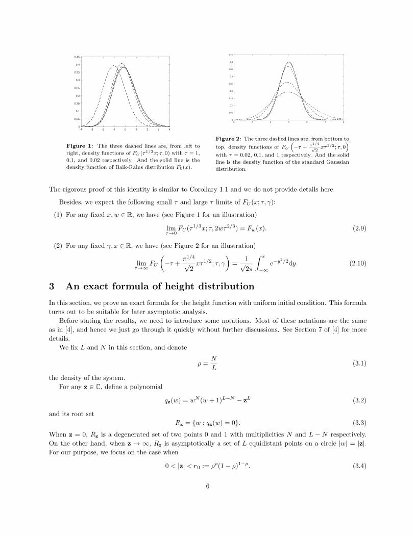
Figure 2: The three dashed lines are, from bottom to

top, density functions of FU

(−τ + π1/4

√2xτ1/2; τ, 0

)with τ = 0.02, 0.1, and 1 respectively. And the solid

line is the density function of the standard Gaussian

distribution.

The rigorous proof of this identity is similar to Corollary 1.1 and we do not provide details here.

Besides, we expect the following small τ and large τ limits of FU (x; τ, γ):

(1) For any fixed x,w ∈ R, we have (see Figure 1 for an illustration)

limτ→0

FU (τ1/3x; τ, 2wτ2/3) = Fw(x). (2.9)

(2) For any fixed γ, x ∈ R, we have (see Figure 2 for an illustration)

limτ→∞

FU

(−τ +

π1/4

√2xτ1/2; τ, γ

)=

1√2π

∫ x

−∞e−y

2/2dy. (2.10)

3 An exact formula of height distribution

In this section, we prove an exact formula for the height function with uniform initial condition. This formula

turns out to be suitable for later asymptotic analysis.

Before stating the results, we need to introduce some notations. Most of these notations are the same

as in [4], and hence we just go through it quickly without further discussions. See Section 7 of [4] for more

details.

We fix L and N in this section, and denote

ρ =N

L(3.1)

the density of the system.

For any z ∈ C, define a polynomial

qz(w) = wN (w + 1)L−N − zL (3.2)

and its root set

Rz = {w : qz(w) = 0}. (3.3)

When z = 0, Rz is a degenerated set of two points 0 and 1 with multiplicities N and L − N respectively.

On the other hand, when z → ∞, Rz is asymptotically a set of L equidistant points on a circle |w| = |z|.For our purpose, we focus on the case when

0 < |z| < r0 := ρρ(1− ρ)1−ρ. (3.4)

6

For such z, Rz contains L −N points in the half plane {w : Re(w) < −ρ} and N points in the second half

plane {w : Re(w) > −ρ}. We denote Rz,left and Rz,right the sets of these L−N and N points respectively.

Then we define

qz,left(w) =∏

u∈Rz,left

(w − u), qz,right(w) =∏

v∈Rz,right

(w − v), (3.5)

which are two monic polynomials with root sets Rz,left and Rz,right respectively. These two functions satisfy

the following equation

qz,left(w)qz,right(w) = qz(w) (3.6)

for all w ∈ C.

For z ∈ C satisfying (3.4) and arbitrary k, ` ∈ Z, we define a kernel K(2)z;k,` acting on `2(Rz,left) as following

K(2)z;k,`(u, u

′) = f2(u)∑

v∈Rz,right

1

(u− v)(u′ − v)f2(v), u, u′ ∈ Rz,left, (3.7)

where the function f2 : Rz → C is defined by

f2(w) = f2(w; k, `) :=

(qz,right(w))

2w−2N−k+2(w + 1)−`+k+1etw

w + ρ, w ∈ Rz,left,(

q′z,right(w))2

w−2N−k+2(w + 1)−`+k+1etw

w + ρ, w ∈ Rz,right.

(3.8)

We also define a function

C(2)N (z; k, `) =

∏u∈Rz,left

(−u)k+N−1∏v∈Rz,right

(v + 1)−`+L−N+ketv∏u∈Rz,left

∏v∈Rz,right

(v − u). (3.9)

K(2)z;k,` and C(2)

N (z; k, `) are the same as K(2)z and C(2)

N (z) in [4] (with ` and k replaced by a and k − N

respectively) but we emphasize the parameters k and ` for our purpose.

Finally we denote ∆k the difference operator

∆kf(k) = f(k + 1)− f(k) (3.10)

for arbitrary function f : Z→ C. For an example, ∆kC(2)N (z; k, `) = C(2)

N (z; k + 1, `)− C(2)N (z; k, `).

Now we state the formula for the distribution function of ht(`).

Theorem 3.1. Suppose ` and b are both integers satisfying b ≡ ` (mod 2). For the N -particle TASEP on

the ring of size L with uniform initial condition, the distribution of the height function is given by

P (ht(`) ≥ b) =(−1)N+1(

LN

) ∮∆k

(C(2)N (z; k, `+ 1) · det

(I +K

(2)z;k,`+1

)) dz

2πizL+1, (3.11)

where

k = 1− b− `2

, (3.12)

and the integral is over an arbitrary simple closed contour which contains 0 inside and lies in an annulus

0 < |z| < r0.

7

Proof. We consider an equivalent model: the TASEP on XN (L). The configuration space XN (L) is defined

by

XN (L) = {(x1, x2, · · · , xN ) ∈ ZN : x1 < x2 < · · · < xN < x1 + L}. (3.13)

The equivalence between TASEP on XN (L) and TASEP with N particles on the ring of size L is as following:

the ring TASEP can be obtained by projecting the particles in TASEP on XN (L) to a ring of size L, and on

the other hand, in the TASEP on a ring if we define xk to be the number of steps the k-th particle moved

plus its initial location, then (x1, · · · , xN ) ∈ XN (L) and we obtain the TASEP on XN (L). See [4] for more

discussions on TASEP on a ring and its equivalent models.

It is easy to see that the uniform initial condition for the TASEP of N particles on a ring of size L

corresponds to the uniform initial condition in the following set

YN (L) = {(y1, y2, · · · , yN ) ∈ ZN : −L+ 1 ≤ y1 < y2 < · · · < yN ≤ 0} (3.14)

in the system of TASEP on XN (L). Moreover, for any Y ∈ YN (L), we have the following relation between

two models 3

P (ht(`) ≥ b in TASEP on the ring with initial configuration Y ) = PY (xk′(t) ≥ a) (3.15)

where

k′ = N

[b− `− 2

2N

]+N + 1− b− `

2,

a = L

[b− `− 2

2N

]+ `+ 1,

(3.16)

and the notations PY , xk′(t) denote the probability of TASEP on XN (L) with initial configuration Y ∈ YN (L)

and the location of the k′-th particle at time t respectively.

Now we sum over all possible initial configurations Y ∈ YN (L) each of which has probability 1

(LN), and

obtain

P(ht(`) ≥ b) =1(LN

) ∑Y ∈YN (L)

PY (xk′(t) ≥ a). (3.17)

On the other hand, the one point distribution function for TASEP on XN (L) with arbitrary initial

condition Y ∈ XN (L) was obtained in [4] (see Proposition 6.1). More explicitly, we have

PY (xk′(t) ≥ a)

=(−1)(k′−1)(N+1)

2πi

∮det

[1

L

∑w∈Rz

wj−i−k′+1(w + 1)yj−j−a+k′+1etw

w + ρ

]Ni,j=1

dz

z1−(k′−1)L,

(3.18)

where the integral is over any simple closed contour with 0 inside. To proceed, we need the following two

lemmas.

Lemma 3.1. Suppose w1, w2, · · · , wN ∈ Rz, then we have∑Y ∈YN (L)

det[wji (wi + 1)yj−j

]Ni,j=1

= det[wj−1i (wi + 1)−N+1

]Ni,j=1

− (−1)N−1z−L det[wji (wi + 1)−N

]Ni,j=1

.

(3.19)

3We first consider the case when 1 ≤ ` ≤ L. In this case, ht(`) = 2J`(t) + h0(`) = 2J`(t) + ` − 2∑`j=1 ηj(0). Therefore

ht(`) ≥ b if and only if J`(t)−∑`j=1 ηj(0) ≥ (b− `)/2, which is further equivalent to xk′ (t) ≥ a. The case when ` ≥ L+ 1 or

` ≤ 0 follows immediately from the fact that ht(`) = ht(`− L) + (L− 2N).

8

Lemma 3.2. (Theorem 7.2 in [4]) Suppose z is in the annulus 0 < |z| < r0 as in (3.4). For any integer k,

we have the following identity4

(−1)(k−1)(N+1)z(k+N−1)L det

[1

L

∑w∈Rz

wj−i−k−N+1(w + 1)−`+ketw

w + ρ

]Ni,j=1

= C(2)N (z; k, `+1)·det

(I +K

(2)z;k,`+1

).

(3.20)

We first assume Lemma 3.1 is true. By inserting (3.18) to (3.17) and then applying Lemma 3.1, we have

P (ht(`) ≥ b) =1(LN

)∆k′(−1)(k′−2)(N+1)

2πi

∮det

[1

L

∑w∈Rz

wj−i−k′+1(w + 1)−N−a+k′+1etw

w + ρ

]Ni,j=1

dz

z1−(k′−2)L.

(3.21)

Note that by using (3.3) this expression is invariant under the following changes: a→ a−L and k′ → k′−N ,

therefore we can replace a by a − L[b−y−2

2N

]= ` + 1 and k′ by k′ − N

[b−y−2

2N

]= k + N . Thus the above

equation equals to

1(LN

)∆k(−1)(k+N−2)(N+1)

2πi

∮det

[1

L

∑w∈Rz

wj−i−k−N+1(w + 1)−`+ketw

w + ρ

]Ni,j=1

dz

z1−(k+N−2)L. (3.22)

By restricting z in the annulus 0 < |z| < r0 and applying Lemma 3.2 we immediately obtain (3.11).

It remains to prove Lemma 3.1.

We take the sum over Y ∈ YN (L) in the following order: yN , yN−1, · · · , y1. It is easy to check that the

summation over Y ∈ YN (L) is equivalent to that over yj : yj−1 +1 ≤ yj ≤ j−N recurrently for j = N, · · · , 2and finally −L + 1 ≤ y1 ≤ 1 − N . Note yj only appears in the j-th column in the determinant on the left

hand side of (3.19). Hence if we take the sum over all possible yj , all other columns in the determinant do

not change except the j-th one. Then for each j = N, · · · , 2, we have the following sum over yj on the j-th

columnj−N∑

yj=yj−1+1

wji (wi + 1)yj−j = wj−1i (wi + 1)−N+1 − wj−1

i (wi + 1)yj−1−(j−1), (3.23)

where the second term is the same as the (i, j − 1) entry thus the determinant does not change if we remove

this term. After taking the sum over yN , · · · , y2, we obtain a new determinant whose first column is the

same as before but the j-th column is wj−1i (wi + 1)−N+1 for all j = N, · · · , 2. Then we take the sum over

y1. Note that the bounds for y1 are −L+ 1 and 1−N . Therefore we have∑Y ∈Y

det[wji (wi + 1)yj−j

]Ni,j=1

= det[wj−1i (wi + 1)−N+1 − δ1(j)wj−1

i (wi + 1)−L]Ni,j=1

= det[wj−1i (wi + 1)−N+1

]Ni,j=1

− det[wj−1i (wi + 1)−N+1−δ1(j)(L−N+1)

]Ni,j=1

,

(3.24)

where δ1(j) is the delta function and we used the linearity of the determinant on the first column in the

second equation. Comparing it with (3.19), it remains to show

det[wj−1i (wi + 1)−N+1−δ1(j)(L−N+1)

]Ni,j=1

= (−1)N−1z−L det[wji (wi + 1)−N

]Ni,j=1

. (3.25)

4The identity in [4] includes an integral over z. However, the proof is still valid if we drop the integral in both sides.

9

By using the fact that (wi+1)L−NwNi = zL and then exchanging the columns, the above equation is further

reduced to

det[wji (wi + 1)−N+1−δN (j)

]Ni,j=1

= det[wji (wi + 1)−N

]Ni,j=1

, (3.26)

which follows from the simple identity[wji (wi + 1)−N+1−δN (j)

]Ni,j=1

=[wji (wi + 1)−N

]Ni,j=1

[δi(j) + δi(j + 1)]Ni,j=1 . (3.27)

4 Asymptotic analysis and proof of Theorem 1.1

In this section, we focus on the asymptotics of the formula (3.11) and prove Theorem 1.1. We will follow

the framework in [4], where they computed the asymptotics of two similar formulas, one of which contains

exactly the same components C(2)N (z; k, `), K

(2)z;k,` and det

(I +K

(2)z;k,`

)as in this paper. However, there are

the following two differences:

(1) In [4], the asymptotics of C(2)N (z; k, `) and det

(I +K

(2)z;k,`

)was obtained with a special choice of param-

eters. More explicitly, the authors considered a case of discrete times t and an order O(L) parameter k.

In this paper, we have a different setting of parameters, in which we let t goes to infinity continuously

and k grows as O(t).

(2) The formula (3.11) in this paper contains a new feature. Namely, we have difference operator ∆k in the

formula, which was not present in [4]. In the asymptotics, this ∆k, after appropriate scaling, converges

to the differentiation with respect to x.

For (1), one can modify the calculations in [4] to the new parameters. However, in this paper we instead

consider a more general setting and find the conditions for parameters such that both C(2)N (z; k, `) and

det(I +K

(2)z;k,`

)converge simultaneously. Then we check our parameters as a special case.

For (2), we need to find the asymptotics of ∆kC(2)N (z; k, `) and ∆k det

(I +K

(2)z;k,`

). The first one can be

obtained straightforward, while the second one requires a bound estimate (uniformly on L and z) of each

term in its expansion, which guarantees the convergence (uniformly on z) of ∆k det(I +K

(2)z;k,`

).

4.1 Setting of the parameters

In this subsection, we list the following general setting of the parameters.

We suppose the density ρ = ρL = NL/L satisfies c1 < ρL < c2 for some fixed positive constants c1, c2.

And we assume

t = tL =τ√

ρL(1− ρL)L3/2 +O(L), (4.1)

for some fixed constant τ > 0. Moreover, suppose ` = `L and k = kL are two integer sequences which are

bounded uniformly by O(L3/2) and satisfy

dist

(`L − (1− 2ρL)tL − γL

L, Z)

= O(L−1/2). (4.2)

andkL + ρL(1− ρL)tL − ρL`L

ρ2/3L (1− ρL)2/3t

1/3L

= x+O(L−1/2), (4.3)

10

where γ = 2wτ2/3 and x are arbitrary fixed real constants, and the notation dist (u,Z) denotes the smallest

distance between u and all integers.

Recall the asymptotics is taken along the line `L = (1− 2ρL)tL + γL, and the asymptotics along the line

`L = (1− 2ρL)tL + (γ + 1)L is the same. See (1.5) and its discussions. The condition (4.2) means that the

points should be asymptotically on the `L = (1− 2ρL)tL + (γ + Z)L lines.

To understand the second condition (4.3), we need to view kL (more precisely kL + NL) as the label of

particle which is at the given location `L at time tL. First we extend the TASEP on a ring to a periodic

TASEP on Z by making infinitely many identical copies of the particles on each interval of length L, more

precisely define xk+N (t) = xk(t) +L for all k and t. With this setting, the labels of particles are in Z instead

of {1, 2, · · · , N}. (4.3) means the label of particle located at site `L at time tL is ρLL − ρL(1 − ρL)tL at

the leading order (more precisely N + ρL`L − ρL(1 − ρL)tL due to our choice of initial labeling: the label

is asymptotically N at site 0 initially), plus an O(t1/3L ) fluctuation term. The term ρL`L (assuming `L > 0,

otherwise considering −`L instead) is asymptotically the number of particles initially in the interval [0, `L],

while ρL(1 − ρL)tL is asymptotically the number of particles jumping through any given site during time

[0, tL].

The above descriptions are in terms of stationary TASEP on a ring with uniform initial condition.

However, recalling the discussions at the beginning of Section 4, the formula arising in step initial condition

contains the same components C(2)N (z; k, `) and det

(I +K

(2)z;k,`

), whose asymptotics can be found within the

same framework. Thus the conditions (4.2) and (4.3) can also be interpreted similarly in terms of TASEP

on a ring with step initial condition.

Now we consider three different choices of parameters satisfying (4.1), (4.2) and (4.3).

The first choice is that we fix the label of particle kL and then let `L and tL go to infinity simultaneously.

This choice corresponds to the case when an observer focuses on a tagged particle. Now we rewrite the

conditions (4.2) and (4.3) as

`L − (1− 2ρL)tL = γL+ jL+O(L1/2) (4.4)

and

`L − (1− ρL)tL = ρ−1kL − xρ−1/3L (1− ρL)2/3t

1/3L , (4.5)

where j = jL is an integer sequence. These two equations imply that

tL =L

ρLj +

γ

ρLL− 1

ρ2L

kL +O(L1/2). (4.6)

Now we want tL grows as (4.1), and hence j grows as[τρ

1/2L (1− ρL)−1/2L1/2

], here the notation [y] denotes

the integer part of y. For simplification, we ignore the O(L1/2) in tL and obtain

tL =L

ρL

[τ√ρL√

1− ρLL1/2

]+

γ

ρLL− 1

ρ2L

kL, (4.7)

which is a time scaling of TASEP on a ring with step initial condition discussed in [4] (with their kL replaced

by kL +NL). See Theorem 3.3 of [4].

The second choice of parameters is that we fix the location `L and let kL and `L goes to infinity simul-

taneously. This choice corresponds to the case when an observer focuses on a fixed location. By a similar

argument as above, we find that tL can be expressed as

L

|1− 2ρL|

[|1− 2ρL|τ√ρL(1− ρL)

L1/2

]− γL

1− 2ρL+

`L1− 2ρL

(4.8)

11

when ρL is of O(1) distance to 1/2. When ρL = 1/2, then the line `L = const is the characteristic line with

a constant shift and this case is reduced to the next one we will discuss later. These scalings were discussed

in [4], see Theorem 3.4 of that paper.

The third choice of parameters is that we fix the line `L − (1 − 2ρL)tL = γL. This is exactly the

choice we pick in Theorem 1.1. It means that an observe moves along the direction of the characteristic

line. In this case, the time parameter tL can grow continuously, and the location `L changes according to

`L − (1 − 2ρL)tL = γL. Finally the label of particle grows by the formula (4.3). Note that in Theorem 1.1

we have the height htL(`L) instead of the label of particles kL, hence to check (4.3) one needs to use the

relation kL = `L−bL2 + 1 in (3.12).

For notation convenience, we will surpass the subscript L in the asymptotic analysis from the next

subsection to the end of Section 4.

4.2 Preliminaries: choice of integral contour and parameter-independent asymp-

totics

In this subsection we follow the setting of [4] (see Section 8) and give the explicit choice of integral contour.

We also give the limit of Rz,left and Rz,right, and asymptocis of some parameter-independent components in

C(2)N (z; k, `). These results are all included in [4] and hence we do not provide details.

In (3.11), we set

zL = (−1)NrL0 z, (4.9)

where z is along any given simple closed contour within the unit disk |z| < 1 and with 0 inside. Then (3.11)

becomes

P (ht(`) ≥ b) =(−1)N+1(

LN

) ∮z−L∆k

(C(2)N (z; k, `+ 1) · det

(I +K

(2)z;k,`+1

)) dz

2πiz, (4.10)

here z = z(z) is any number determined by (4.9). And it is easy to check the integrand above is invariant

for z→ ze2πi/L, and hence the choice of z, provided it satisfies (4.9), does not affect the integral.

We first consider the limits of the nodes sets Rz,left and Rz,right with z scaled as (4.9). It turns out that

after rescaling these nodes sets converge to the sets Sz,left = {ξ : e−ξ2/2 = z,Re ξ < 0} and Sz,right = {ξ :

e−ξ2/2 = z,Re ξ > 0} respectively. The explicit meaning of this convergence is described as below.

Lemma 4.1. (Lemma 8.1 of [4]) Let z be a fixed number satisfying 0 < |z| < 1 and let ε be a real constant

satisfying 0 < ε < 1/2. Set zL = (−1)NrL0 z where r0 = ρρ(1 − ρ)1−ρ. Define the map ML,left from

Rz,left ∩{w : |w + ρ| ≤ ρ

√1− ρN ε/4−1/2

}to Sz,left by

MN,left(w) = ξ, where ξ ∈ Sz,left and

∣∣∣∣ξ − (w + ρ)N1/2

ρ√

1− ρ

∣∣∣∣ ≤ N3ε/4−1/2 logN. (4.11)

Then for large enough N we have:

(a) MN,left is well-defined.

(b) MN,left is injective.

(c) The following relations hold:

S(Nε/4−1)z,left ⊆ I(MN,left) ⊆ S(Nε/4+1)

z,left , (4.12)

where I(MN,left) :=MN,left

(Rz,left ∩ {z : |z + ρ| ≤ ρ

√1− ρN ε/4−1/2}

), the image of the mapMN,left,

and S(c)z,left := Sz,left ∩ {ξ : |ξ| ≤ c} for all c > 0.

12

If we define the mapping MN,right in the same way but replace Rz,left and Sz,left by Rz,right and Sz,right

respectively, the same results hold for MN,right.

Then we consider the limits of qz,left(w), qz,right(w) and the following function

C(2)N,1(z) :=

∏u∈Rz,left

(−u)N∏v∈Rz,right

(v + 1)L−N∏u∈Rz,left

∏v∈Rz,right

(v − u). (4.13)

The first two functions arise from the kernel K(2)z;k,y+1, and the third function C(2)

N,1(z) is part of C(2)N (z; k, `).

The limits of these three functions were obtained in [4] as below.

Lemma 4.2. (Lemma 8.2 of [4]) Suppose z, z and ε satisfy the conditions in Lemma 4.1.

(a) For complex number ξ = ξN satisfying c ≤ |ξ| ≤ N ε/4 with some positive constant c, set wN = wN (ξ) =

−ρ+ ρ√

1− ρξN−1/2. Then for sufficiently large N

qz,left(wN ) = (wN + 1)L−Nehleft(ξ,z)(1 +O(N ε−1/2 logN)) (4.14)

if Re ξ > c, where

hleft(ξ, z) := − 1√2π

∫ −ξ−∞

Li1/2

(ze(ξ2−y2)/2

)dy. (4.15)

Similarly for sufficiently large N

qz,right(wN ) = (−wN )Nehright(ξ,z)(1 +O(N ε−1/2 logN)) (4.16)

if Re ξ < −c, where

hright(ξ, z) := − 1√2π

∫ ξ

−∞Li1/2

(ze(ξ2−y2)/2

)dy. (4.17)

(b) For large enough N we have

C(2)N,1(z) = e2B(z)

(1 +O(N ε−1/2)

), (4.18)

where B(z) = 14π

∫ z0

(Li1/2(y))2

y dy is defined in (2.3).

Finally, we need the expansions of two functions qz(w) and L(w+ρ)w(w+1) along the line Rew = −ρ. These

estimates were obtained in [4], see (9.36) and (9.37) of that paper. Below we gave a quick summary of these

estimates. Write w = −ρ+ ρ√

1− ρξN−1/2, where ξ ∈ iR. It is direct to check that when |ξ| ≤ N ε/4

N log(

1−√

1− ρξN−1/2)

+ (L−N) log

(1 +

ρ√1− ρ

ξN−1/2

)= −1

2ξ2 +

2ρ− 1

3√

1− ρξ3N−1/2 +O(N ε−1),

(4.19)

here and below log denotes the natural logarithm function with the branch cut R≤0.

Together with (3.2) and (4.9), we have for |ξ| ≤ N ε/4

qz(w)

zL= z−1

(1−

√1− ρξN−1/2

)N (1 +

ρ√1− ρ

ξN−1/2

)L−N− 1

=e−ξ

2/2 − zz

(1 +

2ρ− 1

3√

1− ρe−ξ

2/2

e−ξ2/2 − zξ3N−1/2 +O(N ε−1)

).

(4.20)

When |ξ| > N ε/4, it is also easy to check that∣∣∣∣qz(w)

zL

∣∣∣∣ ≥ ecNε/2 (4.21)

13

for some positive constant c.

Similarly, for |ξ| ≤ N ε/4, we have

L(w + ρ)

w(w + 1)= − 1

ρ√

1− ρξN1/2

(1 +

1− 2ρ√1− ρ

ξN−1/2 +O(N−1)

). (4.22)

4.3 Asymptotics of C(2)N (z; k, `)

As we discussed before, the asymptotics of C(2)N (z; k, `) was obtained in [4] with a specific choice of parameters.

The idea is as following: write C(2)N (z; k, `) as C(2)

N,1(z) · C(2)N,2(z; k, `), where C(2)

N,1(z) is defined in (4.13) and

C(2)N,2(z; k, `) :=

∏u∈Rz,left

(−u)k−1∏

v∈Rz,right

(v + 1)−`+ketv. (4.23)

With the parameter setting in [4], they obtained (see Lemma 8.7 in [4])

limN→∞

C(2)N,2(z; k, `) = eτ

1/3xA1(z)+τA2(z)(

1 +O(N ε−1/2)), (4.24)

where A1(z) = − 1√2π

Li3/2(z) and A2(z) = − 1√2π

Li5/2(z) are defined in (2.2). Together with (4.18) in

Lemma 4.2, one has

C(2)N (z; k, `) = eτ

1/3xA1(z)+τA2(z)+2B(z)(

1 +O(N ε−1/2)). (4.25)

The goal of this subsection is to check the proof of (4.24) in [4] also works under the more general

setting (4.1), (4.2) and (4.3). Considering that the asymptotic analysis in [4] was focusing on a different

case which corresponds to the flat initial condition and (4.24) appearing in the step case was only discussed

briefly, and that some parts of the proof will be used in later discussions, we would like to go through the

main steps of the proof of (4.24) with the more general settings in this paper. However, we will not discuss

many details on the calculations unless they are necessary.

First we write the summation in log C(2)N,2(z; k, `) as an integral. By using a residue computation, it is

easy to see that

(k − 1)∑

u∈Rz,left

log(−u) +∑

v∈Rz,right

((−`+ k) log(v + 1) + tv)

=LzL∫ −ρ+i∞

−ρ−i∞(G2(w)−G2(−ρ))

w + ρ

w(w + 1)qz(w)

dw

2πi,

(4.26)

where

G2(w) = (k − 1) log(−w) + (`− k) log(w + 1)− tw. (4.27)

Now we changes variables w = −ρ + ρ√

1− ρξN−1/2 where ξ ∈ iR. Recall (4.21), it is sufficient to

consider the integral over |ξ| ≤ N ε/4 and the error is exponentially small O(e−cNε/2

). With this restriction

and the assumptions that `, k are bounded by O(L3/2), we have

G2(w)−G2(−ρ)

=−k + ρ`− ρ(1− ρ)t√

1− ρN1/2ξ +

(2ρ− 1)k − ρ2`

2(1− ρ)Nξ2 +

−(1− 3ρ+ 3ρ2)k + ρ3`

3(1− ρ)3/2N3/2ξ3 +O(N ε−1/2).

(4.28)

For notation simplification we denote the first three terms a1ξ + a2ξ2 + a3ξ

3. By using the conditions (4.1)-

(4.3), it is easy to see that

a1 = −τ1/3x+O(N−1/2), a2 = O(N1/2), a3 = O(1), − 2(1− 2ρ)a2√1− ρN1/2

+ 3a3 =ρ(−k + ρ`)√

1− ρN3/2= τ +O(N−1/2).

(4.29)

14

Now by plugging (4.28), (4.20), and (4.22) we obtain that (4.26) equals to an exponentially small term

O(e−cNε/2

) plus

−∫ iNε/4

−iNε/4

z(a1ξ2 + a2ξ

3 + a3ξ4)

e−ξ2/2 − z

(1− 2ρ− 1

3√

1− ρe−ξ

2/2

e−ξ2/2 − zξ3N−1/2

)(1 +

1− 2ρ√1− ρ

ξN−1/2

)dξ

2πi+O(N ε−1/2).

(4.30)

By using the symmetry of the integral domain and integrating by parts, it is direct to check that the above

quantity equals to

− a1

∫ iNε/4

−iNε/4

zξ2

e−ξ2/2 − zdξ

2πi−(− 2(1− 2ρ)a2

3√

1− ρN1/2+ a3

)∫ iNε/4

−iNε/4

zξ4

e−ξ2/2 − zdξ

2πi+O(N ε−1/2)

=− a1A1(z) +

(− 2(1− 2ρ)a2√

1− ρN1/2+ 3a3

)A2(z) +O(N ε−1/2)

(4.31)

where A1(z) = − 1√2π

Li3/2(z) =∫

Re ξ=0zξ2

e−ξ2/2−zdξ2πi and A2(z) = − 1√

2πLi3/2(z) = − 1

3

∫Re ξ=0

zξ4

e−ξ2/2−zdξ2πi

are defined in (2.2). Now we insert (4.29) into the above equation, we obtain the right hand side equals to

τ1/3xA1(z) + τA2(z) +O(N ε−1/2). Combing with (4.26), we have (4.24).

4.4 Asymptotics of ∆kC(2)N (z; k, `)

By definition, we have

∆kC(2)N (z; k, `) = C(2)

N (z; k, `)

∏u∈Rz,left

(−u)∏

v∈Rz,right

(v + 1)− 1

. (4.32)

By applying (4.25) and the following Lemma, we obtain

∆kC(2)N (z; k) =

A1(z)√1− ρN1/2

eτ1/3xA1(z)+τA2(z)+2B(z)

(1 +O(N ε−1/2)

), (4.33)

where ε is the same as in the previous subsection.

Lemma 4.3. For any fixed ε satisfying 0 < ε < 1/2, we have∑u∈Rz,left

log(−u) +∑

v∈Rz,right

log(v + 1) =A1(z)√

1− ρN1/2

(1 +O(N ε−1/2)

). (4.34)

Proof. By a residue computation similar to (4.26), we write the left hand side of (4.34) as

LzL∫ −ρ+i∞

−ρ−i∞(log(w/(−ρ))− log((w + 1)/(1− ρ)))

w + ρ

w(w + 1)qz(w)

dw

2πi. (4.35)

The rest of the proof is similar to (4.31) but much easier. We omit the details.

4.5 Asymptotics of det(I + K

(2)z;k,`

)Similarly to C(2)

N (z; k, `), the asymptotics of det(I +K

(2)z;k,`

)was also obtained in [4] with a special setting of

parameters. The argument can apply here for the general settings by a modification. Below we only provide

the main steps and omit the details.

15

By using the property that wN (w + 1)L−N = zL for arbitrary w ∈ Rz, we can rewrite the determinant

as det(I + K

(2)z;k,`

)with the kernel

K(2)z;k,`(u1, u2) = h2(u1)

∑v∈Rz,right

1

(u1 − v)(u2 − v)h2(v)(4.36)

where

h2(w) = h2;k,`(w) =

g2(w)

w + ρ

qz,right(w)2

w2N, w ∈ Rz,left,

g2(w)

w + ρ

q′z,right(w)2

w2N, w ∈ Rz,right,

(4.37)

with

g2(w) = g2;k,`(w) =g2(w)

g2(−ρ)

wjN (w + 1)j(L−N)

(−ρ)jN (−ρ+ 1)j(L−N)(4.38)

and

g2(w) = g2;k,`(w) = w−k+2(w + 1)−`+k+1etw. (4.39)

Here j = jL in (4.38) is an integer sequence satisfying

jL+ `− (1− 2ρ)t− γL = O(L1/2). (4.40)

The existence of such j is guaranteed by (4.2). Moreover, since we assume t and ` are both at most O(L3/2),

we have j ≤ O(L1/2).

Now we consider the asymptotics of h2(w). Write w = −ρ+ ρ√

1− ρξN−1/2. Then we have

g2(w) = e−G2(w)+G2(−ρ) w(w + 1)

−ρ(−ρ+ 1)

(1−

√1− ρξN−1/2

)jN (1 +

ρ√1− ρ

ξN−1/2

)j(L−N)

(4.41)

where G2 is defined in (4.27). If we further assume |ξ| ≤ N ε/4, the asymptotics of g2(w) can be obtained by

using (4.28) and (4.19)

g2(w) = eb1ξ+b2ξ2+b3ξ

3

(1 +O(N ε−1/2)), (4.42)

where

b1 = a1 = −τ1/3x+O(N−1/2),

b2 = a2 −1

2j = −1

2γ +

(1− 2ρ)(ρ`− k − ρ(1− ρ)t)

2ρ(1− ρ)L= −1

2γ +O(N−1/2),

b3 = a3 +2ρ− 1

3√

1− ρjN−1/2 =

(1− 3ρ+ 3ρ2)(ρ`− k)− (2ρ− 1)2ρ(1− ρ)t+O(L)

3ρ3/2(1− ρ)3/2L3/2=τ

3+O(N−1/2).

(4.43)

Here in the second and third equations of (4.43) we used the conditions (4.3) and (4.1). Thus we have

g2(w) = e−τ1/3xξ− γ2 ξ

2+ τ3 ξ

3

(1 +O(N ε−1/2)), (4.44)

Together with Lemma 4.2 (a), we immediately obtain the asymptotics of h2(w) when |w+ρ| ≤ ρ√

1− ρN ε/4.

For the case when |w + ρ| > ρ√

1− ρN ε/4, one can show that h2(w) decays on w ∈ Rz,left and grows on

w ∈ Rz,right exponentially fast as w → ∞. The proof is similar to the case discussed in [4] and we do not

provide details. The explicit asymptotics is described in the following lemma, which was proved for the

special parameters in [4].

Lemma 4.4. (Lemma 8.8 of [4]) Let ε be a fixed constant satisfying 0 < ε < 1/2.

16

(a) When u ∈ Rz,left and |u+ ρ| ≤ ρ√

1− ρN ε/4−1/2, we have

h2(u) =N1/2

ρ√

1− ρξe2hright(ξ,z)− 1

3 τξ3+τ1/3xξ+ 1

2γξ2

(1 +O(N ε−1/2 logN)), (4.45)

where ξ = N1/2(u+ρ)ρ√

1−ρ and hright is defined by (4.17), and the error term O(N ε−1/2 logN) in (4.45) is

independent of u or ξ.

(b) When v ∈ Rz,right and |v + ρ| ≤ ρ√

1− ρN ε/4−1/2, we have

1

h2(v)=ρ3(1− ρ)3/2

ζN3/2e2hleft(ζ,z)+

13 τζ

3−τ1/3xζ− 12γζ

2

(1 +O(N ε−1/2 logN)), (4.46)

where ζ = N1/2(v+ρ)ρ√

1−ρ and hleft is defined by (4.15), and the error term O(N ε−1/2 logN) in (4.46) is

independent of v or ζ.

(c) When w ∈ Rz and |w + ρ| ≥ ρ√

1− ρN ε/4−1/2, we have

h2(w) = O(e−CN3ε/4

), w ∈ Rz,left (4.47)

or1

h2(w)= O(e−CN

3ε/4

), w ∈ Rz,right. (4.48)

Here both error terms O(e−CN3ε/4

) are independent of w.

The Lemmas 4.1 and 4.4 indicate the following result

limn→∞

det(I +K

(2)z;k,`

)= det

(I −K(2)

z;τ1/3x

), (4.49)

where K(2)z;x is an operator on Sz,left as defined in (2.4)5. A rigorous proof needs a uniform bound of the

Fredholm determinant on the left hand side and an error control when we change the space from Rz to Sz,

both of which was considered in [4] for their choice of parameters. However, the argument holds here as well

and hence we omit the details.

4.6 Asymptotics of ∆k det(I + K

(2)z;k

)Similar to the previous subsection, we write ∆k det

(I +K

(2)z;k,`

)as ∆k det

(I + K

(2)z;k,`

).

Before presenting the result, we need the following two lemmas.

Lemma 4.5. For any fixed positive integer m, we have

limn→∞

√1− ρN1/2

∑u1,··· ,um∈Rz,left

∆k det[K

(2)z;k,`(ui, uj)

]mi,j=1

=∑

ξ1,··· ,ξm∈Sz,left

d

dy

∣∣∣∣y=τ1/3x

det[−K(2)

z;y(ξi, ξj)]mi,j=1

.

(4.50)

5Note that hleft(ζ, z) = hright(−ζ, z) = −√

12π

∫−ζ−∞ Li1/2(e−ω

2/2)dω for ζ ∈ Sz,right.

17

Lemma 4.6. There exists some constants C and C ′ which do not depend on z, such that for all positive

integer m we have

N1/2∑

u1,··· ,um∈Rz,left

∣∣∣∣∆k det[K

(2)z;k,`(ui, uj)

]mi,j=1

∣∣∣∣ ≤ 2mCm (4.51)

for all N ≥ C ′.

We first assume both lemmas hold. By using the dominated convergence theorem and the two lemmas

above, we have

limN→∞

√1− ρN1/2∆k det

(I + K

(2)z;k,`

)=∑m≥1

1

m!

d

dy

∣∣∣∣y=τ1/3x

∑ξ1,··· ,ξm∈Sz,left

det[−K(2)

z;y(ξi, ξj)]mi,j=1

. (4.52)

Moreover, the right hand side is uniformly bounded. This further implies ddy

∣∣∣y=τ1/3x

det(I −K(2)

z;y

)is well

defined and uniformly bounded. The above result thus can be written as

limn→∞

√1− ρN1/2∆k det

(I + K

(2)z;k,`

)=

d

dy

∣∣∣∣y=τ1/3x

det(I −K(2)

z;y

)(4.53)

uniformly on z.

Now we prove Lemmas 4.5 and 4.6.

Proof of Lemma 4.5. Recall the definition of K(2)z;k,` in (4.36). It is easy to check that

∆k det[K

(2)z;k,`(ui, uj)

]mi,j=1

=∑

v1,··· ,vm∈Rz,right

∆k det

[h2;k,`(ui)

(ui − vi)(uj − vi)h2;k,`(vi)

]mi,j=1

=∑

v1,··· ,vm∈Rz,right

(m∏i=1

(ui + 1)vi(vi + 1)ui

− 1

)det

[h2;k,`(ui)

(ui − vi)(uj − vi)h2;k,`(vi)

]mi,j=1

.

(4.54)

Here we emphasize the parameters in the function h2(w) to avoid confusion. Hence we have√1− ρN1/2

∑u1,··· ,um∈Rz,left

∆k det[K

(2)z;k,`(ui, uj)

]mi,j=1

=∑

u1,··· ,um∈Rz,left

v1,··· ,vm∈Rz,right

√1− ρN1/2

(m∏i=1

(ui + 1)vi(vi + 1)ui

− 1

)det

[h2;k,`(ui)

(ui − vi)(uj − vi)h2;k,`(vi)

]mi,j=1

.(4.55)

Note that there are only O(L2m) terms in the summation since |Rz| = L, and when |ui + ρ| ≥ ρ√

1− ρN ε/4

or |vi + ρ| ≥ ρ√

1− ρN ε/4 for some i the summand is exponentially small (see Lemma 4.4). Therefore

we can restrict the summation on all ui and vi’s of at most ρ√

1− ρN ε/4 distance to −ρ. We write ui =

−ρ+ ρ√

1− ρξiN−1/2 and vi = −ρ+ ρ√

1− ρζiN−1/2, where |ξi|, |ζi| ≤ N ε/4. Then by applying Lemma 4.4

we have

(4.55)

=∑

ξ1,··· ,ξmζ1,··· ,ζm

(m∑i=1

(ξi − ζi) +O(N ε−1/2)

)det

[eφright(ξi)−φleft(ζi)

ξiζi(ξi − ζi)(ξj − ζi)+O(N ε−1/2 logN)

]mi,j=1

+O(e−cNε/2

),

(4.56)

18

where the summation is over all possible ξi and ζi such that |ξi|, |ζi| ≤ N ε/4 and−ρ+ρ√

1− ρξiN−1/2 ∈ Rz,left

and −ρ+ ρ√

1− ρζiN−1/2 ∈ Rz,right for all i = 1, · · · ,m. And

φright(ξ) := 2hright(ξ, z)−1

3τξ3 +

1

2γξ2 + τ1/3xξ,

φleft(ζ) := −2hleft(ζ, z)−1

3τζ3 +

1

2γζ2 + τ1/3xζ,

(4.57)

for ξ and ζ satisfying Re ξ < 0 and Re ζ > 0. Recall that the error terms in (4.56) are all uniformly on

ξi and ηi (see Lemma 4.4), and note that there are at most O(N ε/2) elements by Lemma 4.1 part (c).

Therefore (4.56) equals to

∑ξ1,··· ,ξmζ1,··· ,ζm

m∑i=1

(ξi − ζi) det

[eφright(ξi)−φleft(ζi)

ξiζi(ξi − ζi)(ξj − ζi)

]mi,j=1

+O(N (m+2)ε−1/2). (4.58)

Now by using Lemma 4.1 we know that these ξi and ζi’s are chosen from a perturbation of I(MN,left)

and I(MN,right), the images of MN,left and MN,right respectively, see Lemma 4.1. The perturbation size is

uniformly bounded by N3ε/4−1/2 logN . Similar to the reasoning from (4.56) to (4.58), we can replace (4.58)

by ∑ξ1,··· ,ξm∈I(MN,left)ζ1,··· ,ζm∈I(MN,right)

m∑i=1

(ξi − ζi) det

[eφright(ξi)−φleft(ζi)

ξiζi(ξi − ζi)(ξj − ζi)

]mi,j=1

+O(N (m+2)ε−1/2). (4.59)

If we choose ε small such that (m+ 2)ε < 1/2, then the above quantity converges to

∑ξ1,··· ,ξm∈Sz,leftζ1,··· ,ζm∈Sz,right

m∑i=1

(ξi − ζi) det

[eφright(ξi)−φleft(ζi)

ξiζi(ξi − ζi)(ξj − ζi)

]mi,j=1

. (4.60)

Finally we check that (4.60) equals to the right hand side of (4.50). This follows from the facts that

hright(ξ, z) = − 1√2π

∫ ξ−∞ Li1/2(e−ω

2/2)dω for all ξ ∈ Sz,left, and hleft(ζ, z) = − 1√2π

∫ −ζ−∞ Li1/2(e−ω

2/2)dω for

all ζ ∈ Sz,right, and that Sz,right = −Sz,left.

Proof of Lemma 4.6. In this proof, we need the following result.

Claim 4.1. There exist a positive constant C and C ′ uniformly on z such that∑u1∈Rz,left

√ ∑u2∈Rz,left

|A(u1, u2)|2 ≤ C (4.61)

for all N ≥ C ′, where

A(u1, u2) :=√|h2(u1)h2(u2)|E(u1)E(u2)

∑v∈Rz,right

|E(v)|2

|u1 − v||u2 − v||h2(v)|(4.62)

and

E(w) := 1 +ρ|w + 1|

(1− ρ)|w|+

(1− ρ)|w|ρ|w + 1|

+N1/2

(∣∣∣∣ (1− ρ)w

ρ(w + 1)+ 1

∣∣∣∣+

∣∣∣∣ρ(w + 1)

(1− ρ)w+ 1

∣∣∣∣) . (4.63)

Proof of Claim 4.1. Note that E(w) is always positive and bounded by c1N1/2 + c2 uniformly on Rz. On

the other hand, h2(u) and h2(v)−1 are exponentially small when u ∈ Rz,left , v ∈ Rz,right are of distance

19

≥ O(N ε/4−1/2), see Lemma 4.4 (c). Thus it is sufficient to prove the following inequality

∑u1∈Rz,left

|u1+ρ|≤Nε/4−1/2

√√√√√√√√ ∑u2∈Rz,left

|u2+ρ|≤Nε/4−1/2

|h2(u1)h2(u2)E(u1)2E(u2)2|

∑v∈Rz,right

|v+ρ|≤Nε/4−1/2

|E(v)|2|u1 − v||u2 − v||h2(v)|

2

≤ C.

(4.64)

On the other hand, it is easy to check that

E(−ρ+ ρ√

1− ρξN−1/2) = 3 +2√

1− ρ|ξ|+O(N ε−1/2) ≤ 3 + C1|ξ|+O(N ε−1/2), (4.65)

uniformly for all |ξ| ≤ N ε/4, here C1 is a constant independent of N (recall that ρ = ρL ∈ (c1, c2) depends

on L). We denote

E(−ρ+ ρ√

1− ρξN−1/2) := the right hand side of (4.65). (4.66)

Then (4.64) is reduced to

∑u1∈Rz,left

|u1+ρ|≤Nε/4−1/2

√√√√√√√√ ∑u2∈Rz,left

|u2+ρ|≤Nε/4−1/2

|h2(u1)h2(u2)E(u1)2E(u2)2|

∑v∈Rz,right

|v+ρ|≤Nε/4−1/2

|E(v)|2|u1 − v||u2 − v||h2(v)|

2

≤ C.

(4.67)

Using Lemmas 4.1 and 4.4, the left hand side of (4.67) converges to

∑ξ1∈Sz,left

√√√√√ ∑ξ2∈Sz,right

∣∣∣∣∣eφright(ξ1)+φright(ξ2)

ξ1ξ2

∣∣∣∣∣ ∑ζ∈Sz,right

|e−φleft(ζ)||ξ1 − ζ||ξ2 − ζ|

2

, (4.68)

as N → ∞, where φright(ξ) := φright(ξ) + 2 log (3 + C1|ξ|) and φleft(ζ) := φleft(ζ) − 2 log (3 + C1|ξ|). The

rigorous proof of this convergence is similar to that of Lemma 4.5 and hence we do not provide details. Also

it is easy to see that (4.68) is finite. Therefore (4.67) holds for sufficiently large N .

Now we prove Lemma 4.6. This idea is to express the summand on the left hand side of (4.51) as a sum

of determinants det[A(n)(ui, uj)

]where A(n) has similar structure of A in Claim 4.1, and then apply the

Hadamard’s inequality.

The first step is to write

det[K

(2)z;k,`(ui, uj)

]mi,j=1

=∑

v1,··· ,vm∈Rz,right

det

[ √h2;k,`(ui)

√h2;k,`(uj)

(ui − vi)(uj − vi)h2;k,`(vi)

]mi,j=1

(4.69)

by using a conjugation, here√h2;k,`(ui) is the square root function with any fixed branch cut. Denote

Hk,`(u, u′; v) =

√h2;k,`(u)

√h2;k,`(u′)

(u− v)(u′ − v)h2;k,`(v). (4.70)

20

Similarly to (4.54), we have

N1/2∆k det[K

(2)z;k,`(ui, uj)

]mi,j=1

=N1/2∑

v1,··· ,vm∈Rz,right

(m∏i=1

(ui + 1)vi(vi + 1)ui

− 1

)det [Hk,`(ui, uj ; vi)]

mi,j=1

=

m∑n=1

∑v1,··· ,vm∈Rz,right

N1/2

(−ρ(un + 1)

(1− ρ)un− 1

) n−1∏i=1

−ρ(ui + 1)

(1− ρ)uidet

[(1− ρ)viHk,`(ui, uj ; vi)

−ρ(vi + 1)

]mi,j=1

+

m∑n=1

∑v1,··· ,vm∈Rz,right

N1/2

(1− −ρ(vn + 1)

(1− ρ)vn

) n−1∏i=1

−ρ(vi + 1)

(1− ρ)videt

[(1− ρ)viHk,`(ui, uj ; vi)

−ρ(vi + 1)

]mi,j=1

=

m∑n=1

det[A(n)(ui, uj)

]mi,j=1

+

m∑n=1

det[A(n)(ui, uj)

]mi,j=1

,

(4.71)

where

A(n)(ui, uj) =

−ρ(ui + 1)

(1− ρ)ui

∑v∈Rz,right

(1− ρ)vHk,`(ui, uj ; v)

−ρ(v + 1), 1 ≤ i ≤ n− 1,

N1/2

(−ρ(un + 1)

(1− ρ)un− 1

) ∑v∈Rz,right

(1− ρ)vHk,`(ui, uj ; v)

−ρ(v + 1), i = n,

∑v∈Rz,right

(1− ρ)vHk,`(ui, uj ; v)

−ρ(v + 1), n+ 1 ≤ i ≤ m,

(4.72)

and

A(n)(ui, uj) =

∑v∈Rz,right

Hk,`(ui, uj ; v), 1 ≤ i ≤ n− 1,

∑v∈Rz,right

N1/2

((1− ρ)v

−ρ(v + 1)− 1

)Hk,`(ui, uj ; v), i = n,

∑v∈Rz,right

(1− ρ)vHk,`(ui, uj ; v)

−ρ(v + 1), n+ 1 ≤ i ≤ m.

(4.73)

It is easy to check that |A(n)(ui, uj)| and |A(n)(ui, uj)| are bounded by |A(ui, uj)| defined in the Claim 4.1.

By Hadamard’s inequality, we have∣∣∣∣det[A(n)(ui, uj)

]mi,j=1

∣∣∣∣ ≤ m∏i=1

√ ∑1≤j≤m

|A(n)(ui, uj)|2 ≤m∏i=1

√ ∑u′∈Rz,left

|A(ui, u′)|2 (4.74)

for all distinct u1, · · · , um ∈ Rz,left. As a result,

∑u1,··· ,um∈Rz,left

all distinct

∣∣∣∣det[A(n)(ui, uj)

]mi,j=1

∣∣∣∣ ≤ ∑u1,··· ,um∈Rz,left

m∏i=1

√ ∑u′∈Rz,left

|A(ui, u′)|2

=

∑u∈Rz,left

√ ∑u′∈Rz,left

|A(u, u′)|2

m

≤ Cm(4.75)

21

by the Claim 4.1. Similarly we have ∑u1,··· ,um∈Rz,left

all distinct

∣∣∣∣det[A(n)(ui, uj)

]mi,j=1

∣∣∣∣ ≤ Cm. (4.76)

Also note that ∆k det[K

(2)z;k,`(ui, uj)

]mi,j=1

= 0 if ui = uj for some 1 ≤ i < j ≤ m. By combing (4.71), (4.75)

and (4.76) we obtain (4.51).

4.7 Proof of Theorem 1.1

Now we prove Theorem 1.1(a). By using the estimates (4.25), (4.33), (4.49) and (4.53), we obtain

limn→∞

√1− ρN1/2∆k

(C(2)N (z; k) · det

(I +K

(2)z;k

))=

d

dy

∣∣∣∣y=τ1/3x

(eyA1(z)+τA2(z)+2B(z) det

(I −K(2)

z;y

)).

(4.77)

Furthermore, by the discussions below (4.49) and Lemma 4.6, we know the left hand side of (4.77) is uniformly

bounded on z.

On the other hand, by using the sterling’s formula and (4.9), we obtain

(−1)N(LN

) 1√1− ρN1/2zL

=N !(L−N)!

L!ρN (1− ρ)L−N√

1− ρN1/2z=

√2π

z(1 +O(N−1)). (4.78)

Theorem 1.1 follows immediately by inserting the above two estimates into (4.10).

A Tail bound of the limiting distribution

In this appendix, we give some tail bounds related to the function FU . These estimates are not optimal,

however, they are sufficient to show that (1) FU (x; τ, γ) is a distribution function, and (2) the n-th moments

ofhtL (`L)−(1−2ρL)`L−2ρL(1−ρL)tL

−2ρ1/2L (1−ρL)1/2L1/2

converges to that of∫R x

ndFU (x; τ, γ) for any finite n as L→∞, here ρL, `L

and tL are defined in Theorem 1.1. The second statement follows in the same way as Theorem 1 in [3].

For simplification we only consider the case when τ = 1. For other values of τ , the statements and proofs

are the same (with different constants).

Define

F(L)U (x) := P

(htL(`L)− (1− 2ρL)`L − 2ρL(1− ρL)tL

−2ρ2/3L (1− ρL)2/3t

1/3L

≤ x

)(A.1)

and

G(L)U (x) :=

(−1)NL+1(LNL

) ∮C(2)N (z; kL, `L + 1) · det

(I +K

(2)z;kL,`L+1

) dz

2πizL+1(A.2)

where the parameters and notations are the same as in Theorem 1.1, and we surpass the parameters τ = 1

and γ in the indices for simplification, and

kL = 1 + ρL`L − ρL(1− ρL)tL + xρ2/3L (1− ρL)2/3t

1/3L . (A.3)

By using Theorem 3.1, it is easy to check

F(L)U (x) =

t−1/3L

ρ2/3L (1− ρL)2/3

d

dxG

(L)U (x) (A.4)

where x is an point satisfying x = x+O(t−1/3L ).

22

Proposition A.1. (Left tail bound of F(L)U ) There exist constants α > 0, c > 0, C > 0 and C ′ > 0, such

that

F(L)U (x) ≤ e−c|x|

α

(A.5)

for all x ≤ −C and L ≥ C ′|x|.

Proposition A.2. (Right tail bound of G(L)U ) There exist constants α > 0, c > 0, C > 0 and C ′ > 0, such

that ∣∣∣∣∣x+ 1−t−1/3L

ρ2/3L (1− ρL)2/3

G(L)U (x)

∣∣∣∣∣ ≤ e−cxα (A.6)

for all x ≥ C and L ≥ C ′x6.6

Although we use the same notations of constants α, c, C and C ′ in the above two propositions, their

values are not the same.

We also remark that these two propositions are analogous to Proposition 1 and 2 in [3].

A.1 Proof of Proposition A.1

The idea of the proof is to map the periodic TASEP to the periodic directed last passage percolation (DLPP).

The relation was discussed in [4] and [5] and we refer the readers to Section 3.1 of [5] for more details. Here

we just give a brief description.

We first introduce the periodic TASEP. This is equivalent to TASEP on XN (L) except we have infinitely

many copies of particles, which satisfy xk+N (t) = xk(t) + L for all k ∈ Z.

Similarly to the mapping between the infinite TASEP and usual DLPP, see [11], there is a mapping from

periodic TASEP to periodic DLPP described as following: Let v = (L−N,−N) be the period vector, and

Γ be a lattice path with lower left corners (i+ xN+1−i(0), i) for i ∈ Z. It is easy to check that Γ is invariant

if translated by v. Let w(q) be random exponential variables with parameter 1 for all lattice points q which

are on the upper right side of Γ. We require w(q) = w(q + v) for all q. Except for this restriction, all w(q)

are independent. We then define

Hp(q) = maxπ

∑r∈π

w(r) (A.7)

where the maximum is over all the possible up/right lattice paths from p to q. We also define

HΓ(q) = maxp

Hp(q). (A.8)

Now we are ready to introduce the relation between particle location in periodic DLPP and last passage

time in periodic DLPP, see (3.7) in [5],

Pv (xk(t) ≥ a) = Pv (HΓ(N + a− k,N + 1− k) ≤ t) , (A.9)

where we use the notation Pv to denote the probability functions in periodic TASEP and the equivalent

periodic DLPP model. Using (A.9) and the relation between height function ht(`L) and the particle location

xk(t), see (3.15), it is a direct to show the following

F(L)U (x) = Pv (HΓ(q) ≤ tL) (A.10)

where q = (q1,q2) with

q1 = (1− ρL)2tL + γ(1− ρL)L− xρ2/3L (1− ρL)2/3t

1/3L ,

q2 = ρ2LtL − γρLL− xρ

2/3L (1− ρL)2/3t

1/3L .

(A.11)

6For general τ , the term x+ 1 in (A.6) should be replaced by x+ τ .

23

The rest of this section is to show that there exist constants α > 0, c > 0, C > 0, and C ′ > 0, such that

Pv (HΓ(q) ≤ tL) ≤ e−c|x|α

(A.12)

for all x < −C and L ≥ C ′|x|. Then Proposition A.1 follows immediately.

The idea to prove (A.12) is to compare the periodic DLPP with the usual DLPP. This idea was applied in

[5] for periodic TASEP in sub-relaxation time scale. In the case we consider in this paper, we need a relaxation

time analogous of the argument and hence a modification is needed. We first introduce some known results

on DLPP model. The probability space for DLPP is that all the lattice points q are associated with an

i.i.d. exponential random variable w(q), we use P to denote the probability associated to this space. Similarly

to the periodic DLPP, we denote Gp(q) the last passage time from p to q, and GΛ(q) the last passage time

from the lattice path Λ to q. Finally we define B(c1, c2) := {q = (q1,q2) ∈ Z2≥0; c1q1 ≤ q2 ≤ c2q1} for

arbitrary constants c1, c2 satisfying 0 < c1 < c2. From now on we fix these two constants c1 and c2. It is

known that [11]

lim|q|→∞

q∈B(c1,c2)

P(G(q)− d(q)

s(q)≤ x

)= FGUE(x), (A.13)

where d(q) = (√q1 +

√q2)2 and s(q) = (q1q2)−1/6(

√q1 +

√q2)4/3. The following tail estimate is also

needed, which is due to [1, 3],

P(G(q)− d(q)

s(q)≤ −y

)≤ e−c3y (A.14)

for sufficiently large y ≥ C1 and q ∈ B(c1, c2) satisfying |q| ≥ C ′1. Here c3, C1 and C ′1 are constants only

depend on c1 and c2. The last result in DLPP we need is about the transversal fluctuations. Define Bpq(y)

to be the set of all lattice points r satisfying

dist (r,pq) ≤ y|q− p|2/3. (A.15)

We also define πmaxp (q) to be the maximal path from p to q in the usual DLPP. The following transversal

fluctuation estimate is currently known: There exist constants c4, C2 and C ′2 such that

P(πmax0 (q) ⊆ B0q(y)

)≥ 1− e−c4y (A.16)

for all y ≥ C2 and and q ∈ B(c1, c2) satisfying |q| ≥ C ′2. The analog of this estimate in Poissonian version of

DLPP was obtained in [7] and their idea can be applied in the exponential case similarly. We hence do not

provide a proof here, instead we refer the readers to a forthcoming paper [13] by Nejjar for more discussions.

Now we use (A.14) and (A.16) to prove (A.12). We pick k+1 equidistant points 0 = q(0),q(1) · · · ,q(k) = q

on the line 0q such that

dist(v,0q

)≥ C2|q(i+1) − q(i)|2/3, i = 0, 1, · · · , k − 1, (A.17)

here k is some large parameter which will be decided later. Note that dist(v,0q

)= O(|q|2/3), hence the

above inequality is satisfied as long as k is greater than certain constant.

Now note that HΓ(q) ≥ H(1,1)(q) = H0(q) +O(1) since (1, 1) is at the upper right side of to the initial

contour Γ by definition, and H0(q) ≥∑k−1i=0 Hq(i)(q(i+1)), therefore

Pv (HΓ(q) ≤ tL) ≤ kPv

(H0(q(1)) ≤ tL/k

). (A.18)

On the other hand, by using (A.16) we know that

Pv

(H0(q(1)) ≤ tL/k

)≤ P

(G0(q(1)) ≤ tL/k

)+ e−c4k

2/3|q|−2/3dist (v,0q) (A.19)

24

provided |q| ≥ C ′2k. Finally, by inserting (A.11) and then applying (A.14), we have

P(G0(q(1)) ≤ tL/k

)≤ e−c5k

−2/3|x| (A.20)

provided |q| ≥ C ′1k and x < −C, where c5 and C are constants. By combing (A.18), (A.19) and (A.20), we

obtain

Pv (HΓ(q) ≤ tL) ≤ ke−c5k−2/3|x| + ke−c4k

2/3|q|−2/3dist (v,0q) (A.21)

Finally we pick k = |x| and (A.12) follows immediately.

A.2 Proof of Proposition A.2

The proof is similar to that of Theorem 1.1 but we do not need to handle the difference operator. We only

provide the main ideas here.

First we do the same change of variables as in (4.10) and write

G(L)U (x) =

(−1)N+1(LN

) ∮z−L

(C(2)N (z; k, `+ 1) · det

(I +K

(2)z;k,`+1

)) dz

2πiz. (A.22)

Now we assume x is large and pick z on the following circle

|z| = e−x. (A.23)

With this choice of z, by using a similar argument as in Section 4.3 we have

C(2)N (z; k, `+ 1) = exA1(z)+A2(z)+2B(z)(1 +O(L−1/3)) =

(1− 1√

2π(x+ 1)z

)(1 +O(L−1/3)) +O(ze−cx)

(A.24)

provided L� x6. By tracking the error terms, the term O(L−1/3) is analytic in z and can be expressed as

c+ c′z +O(z2L−1/3) with c, c′ both bounded by O(L−1/3).

And similarly to Section 4.5, we write det(I +K

(2)z;k,`+1

)as det

(I + K

(2)z;k,`

)whose kernel is defined

in (4.36). By a similar argument as Lemma 4.4, one can show that the kernel decays exponentially∣∣∣K(2)z;k,`(ξ, η)

∣∣∣ ≤ e−c(Re(− 13 ξ

3+xξ)+(− 13η

3+xη)) (A.25)

for all ξ, η ∈ Sz,left and sufficiently large x. Here c > 0 is a constant. The heuristic argument is as following:

Suppose ξ = a+ ib ∈ Sz,left with a < 0, then a2 − b2 = 2x by (A.23). It is a direct to show that the leading

term in the exponent of h(u) in Lemma 4.4 (a) (after dropping the term 12γξ

2, whose real part is independent

of ξ and hence cancels with the counterpart from 1/h(v)) is

Re

(−1

3ξ3 + xξ

)=

2

3a3 − xa ≤ 1

3xa ≤ −2

3x3/2 � 0. (A.26)

Similar estimates for the 1/h(v) in Lemma 4.4 (b) holds. Therefore we have (A.25). Finally, by using (A.25)

and (A.26), it is a direct to prove that

det(I + K

(2)z;k,`

)= 1 +O(e−cx

3/2

) (A.27)

for a different positive constant c. Since the above argument is similar to that in Section 4.5, we do not

provide details.

Finally by combing (4.78), (A.24) and (A.27), also noting that zL = (−1)NrL0 z, we obtain that

G(L)U (x) =

√ρL(1− ρL)L1/2

(x+ 1 +O(e−cx)

). (A.28)

Hence we obtain Proposition A.2.

25

References

[1] J. Baik, G. B. Arous, and S. Peche. Phase transition of the largest eigenvalue for nonnull complex

sample covariance matrices. Ann. Probab., 33(5):1643–1697, 2005.

[2] J. Baik, P. L. Ferrari, and S. Peche. Limit process of stationary TASEP near the characteristic line.

Comm. Pure Appl. Math., 63(8):1017–1070, 2010.

[3] J. Baik, P. L. Ferrari, and S. Peche. Convergence of the two-point function of the stationary TASEP.

In Singular phenomena and scaling in mathematical models, pages 91–110. Springer, Cham, 2014.

[4] J. Baik and Z. Liu. Fluctuations of TASEP on a ring in relaxation time scale. 2016. arXiv:1605.07102.

[5] J. Baik and Z. Liu. Tasep on a ring in sub-relaxation time scale. 2016. arXiv:1608.08263.

[6] J. Baik and E. M. Rains. Limiting distributions for a polynuclear growth model with external sources.

J. Statist. Phys., 100(3-4):523–541, 2000.

[7] R. Basu, V. Sidoravicius, and A. Sly. Last Passage Percolation with a Defect Line and the Solution of

the Slow Bond Problem. arxiv:1408.3464.

[8] B. Derrida and J. L. Lebowitz. Exact large deviation function in the asymmetric exclusion process.

Phys. Rev. Lett., 80(2):209–213, 1998.

[9] P. L. Ferrari and H. Spohn. Scaling limit for the space-time covariance of the stationary totally asym-

metric simple exclusion process. Comm. Math. Phys., 265(1):1–44, 2006.

[10] L.-H. Gwa and H. Spohn. Six-vertex model, roughened surfaces, and an asymmetric spin Hamiltonian.

Phys. Rev. Lett., 68(6):725–728, 1992.

[11] K. Johansson. Shape fluctuations and random matrices. Comm. Math. Phys., 209(2):437–476, 2000.

[12] P. Meakin, P. Ramanlal, L. M. Sander, and R. C. Ball. Ballistic deposition on surfaces. Phys. Rev. A,

34:5091–5103, Dec 1986.

[13] P. Nejjar. Transition to shock fluctuations in TASEP. Upcoming.

[14] M. Prahofer and H. Spohn. Current fluctuations for the totally asymmetric simple exclusion process. In

In and out of equilibrium (Mambucaba, 2000), volume 51 of Progr. Probab., pages 185–204. Birkhauser

Boston, Boston, MA, 2002.

[15] S. Prolhac. Finite-time fluctuations for the totally asymmetric exclusion process. Phys. Rev. Lett.,

116:090601, 2016.

26