Embed Size (px)
Citation preview
2018 Volume 26 No.1-2
GENERAL MATHEMATICS
EDITOR-IN-CHIEF
Daniel Florin SOFONEA
ASSOCIATE EDITOR
Ana Maria ACU
HONORARY EDITOR
Dumitru ACU
EDITORIAL BOARD
Heinrich Begehr Andrei Duma Dumitru Gaspar
Shigeyoshi Owa Dorin Andrica Hari M. Srivastava
Malvina Baica Vasile Berinde Piergiulio Corsini
Vijay Gupta Gradimir V. Milovanovic Claudiu Kifor
Detlef H. Mache Aldo Peretti Adrian Petrusel
SCIENTIFIC SECRETARY
Emil C. POPA
Nicusor MINCULETE
Ioan TINCU
Augusta RATIU
EDITORIAL OFFICE
DEPARTMENT OF MATHEMATICS AND INFORMATICS
GENERAL MATHEMATICS
Str.Dr. Ion Ratiu, no. 5-7 550012 - Sibiu, ROMANIA
Electronical version: http://depmath.ulbsibiu.ro/genmath/

Contents
V. Gupta, Some Examples of Genuine Approximation Operators . . . . 3
A. K. Wanas, B. A. Frasin, Applications of Fractional Calculus for a
Certain Subclass of Multivalent Analytic Functions on Complex Hilbert
Space . . . . . . . . . . . . . . . . . . . . . . . . . . . . . . . . . . . . . . . . . . . . . . . . . . . . . . . . . . . . . . 11
K. R. Karthikeyan, K. Srinivasan, K. Ramachandran, Some Classes
Of Multivalent Starlike Functions With Respect To Symmetric
Conjugate Points . . . . . . . . . . . . . . . . . . . . . . . . . . . . . . . . . . . . . . . . . . . . . . . . . . . 25
U. Abel, G. Arends, A remark on some combinatorial identities . . 35
M. Cakmak, Refinements of Bullen-Type Inequalities for Different Kind
of Convex Functions via Riemann-Liouville Fractional Integrals Involving
Gauss Hypergeometric Function . . . . . . . . . . . . . . . . . . . . . . . . . . . . . . . . . . . . 41
A. Ratiu, D. I. Duca, Second Order Approximated Semi-Infinite
Optimization Problems . . . . . . . . . . . . . . . . . . . . . . . . . . . . . . . . . . . . . . . . . . . . . 57
H. Bouhadjera, Common Fixed Points for Two Mappings . . . . . . . . .79
Shyam Lal, Rakesh, Legendre Wavelet approximation of a Function
f with its third derivative f (3) belonging to Lipschitz class of order
0 < α ≤ 1 . . . . . . . . . . . . . . . . . . . . . . . . . . . . . . . . . . . . . . . . . . . . . . . . . . . . . . . . . 101
K. Sarkar, K. Tiwary, Common Coupled Coincidence Point in Cone
Metric Space . . . . . . . . . . . . . . . . . . . . . . . . . . . . . . . . . . . . . . . . . . . . . . . . . . . . . . 127

General Mathematics Vol. 26, No. 1-2 (2018), 3–9
Some Examples of Genuine Approximation Operators 1
Vijay Gupta
Abstract
In the present paper we provide some examples of operators, which pre-serve constant as well as linear functions and establish their moments in termsof hypergeometric and confluent hypergeometric series. We also establish thequantitative estimate for the difference of Srivastava-Gupta operators and Mas-troianni operators.
2010 Mathematics Subject Classification: 41A25, 41A30.Key words and phrases: Srivastava-Gupta operators, Mastroianni operators,
genuine operators, hypergeometric series, difference of operators.
1 Introduction
In [12] Srivastava-Gupta proposed the summation-integral type operators, which aredefined by
Gn,c(f, x) = n∞∑k=1
pn,k(x, c)
∫ ∞0
pn+c,k−1(t, c)f(t)dt
+pn,0(x, c)f(0),(1)
where
pn,k(x, c) =(−x)k
k!φ(k)n,c(x)
with the following special cases:
• If c = 0 and φn,c(x) = e−nx then we get pn,k(x, 0) = e−nx (nx)k
k! ,
• If c ∈ N and φn,c(x) = (1+cx)−n/c, then we obtain pn,k(x, c) = (n/c)kk!
(cx)k
(1+cx)nc +k ,
1Received 10 January, 2018Accepted for publication (in revised form) 23 February, 2018
3
4 Vijay Gupta
• If c = −1 and φn,c(x) = (1− x)n then pn,k(x,−1) =(nk
)xk(1− x)n−k.
In the last case c = −1, we have x ∈ [0, 1], while for c ∈ N ∪ {0}, we havex ∈ [0,∞). In [2], [9] and [13] some approximation properties of these operatorsand their variants have been discussed. The r-th (r ∈ N) order moments of (1) wither(t) = tr, satisfy the relation:
Gn,c(er, x) =
{nx·r!
(n−c)(n−2c)···(n−rc) 2F1
(nc + 1, 1− r; 2;−cx
), c ∈ N ∪ {−1},
nx.r!nr 1F1(1− r; 2;−nx), c = 0.
From the above hypergeometric and confluent hypergeometric series representationof the moments, one can see that the operators defined by (1) preserve only the con-stant functions. Also, for n > c(r+ 1) the moments satisfy the following recurrencerelation:
[n− c(r + 1)]Gn,c(er+1, x) = (nx+ r)Gn,c(er, x) + x(1 + cx)G′n,c(er, x).
For some other sequences of similar type linear positive operators, we refer the read-ers to [3], [4], [6] and [8] etc. Here we give some examples of genuine operators and inlast section, we find the difference of Srivastava-Gupta operators with Mastroiannioperators.
2 Genuine operators and Moments
In this section, we provide some examples of operators, which reproduce the linearfunctions, we may say such operators as genuine operators. Although for the casec = 0, the original operators (1) are genuine operators, but for all other cases, onemay consider the following:
Example 1 For c ∈ N ∪ {0}, we introduce
Vn,c(f, x) = n
∞∑k=1
pn−c,k(x, c)
∫ ∞0
pn+c,k−1(t, c)f(t)dt
+pn−c,0(x, c)f(0),
where pn,k(x, c) is as defined in (1) above. The two cases mentioned above providewell known Phillips operators and the genuine Baskakov-Durrmeyer type operatorsrespectively. For c = −1 the operators take the form:
Vn,−1(f, x) = nn∑
k=1
pn+1,k(x,−1)
∫ 1
0pn−1,k−1(t,−1)f(t)dt
+pn+1,0(x,−1)f(0) + pn+1,n+1(x,−1),
The r-th (r ∈ N) order moments of the operators Vn,c, in terms of hypergeometricfunction satisfy
Vn,c(er, x) = xΓ((n/c)− r)Γ(r + 1)
Γ((n/c)− 1).cr−12F1
(nc, 1− r; 2;−cx
), c ∈ N ∪ {−1}.
Genuine Approximation Operators 5
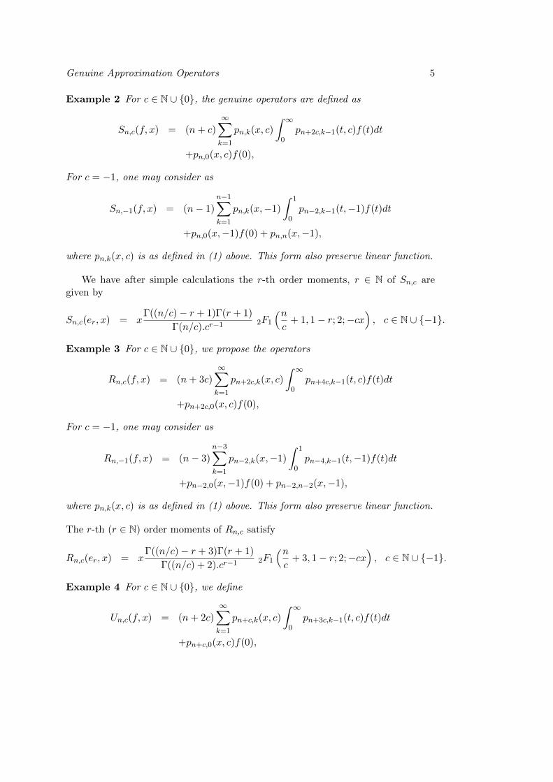
Example 2 For c ∈ N ∪ {0}, the genuine operators are defined as
Sn,c(f, x) = (n+ c)∞∑k=1
pn,k(x, c)
∫ ∞0
pn+2c,k−1(t, c)f(t)dt
+pn,0(x, c)f(0),
For c = −1, one may consider as
Sn,−1(f, x) = (n− 1)
n−1∑k=1
pn,k(x,−1)
∫ 1
0pn−2,k−1(t,−1)f(t)dt
+pn,0(x,−1)f(0) + pn,n(x,−1),
where pn,k(x, c) is as defined in (1) above. This form also preserve linear function.
We have after simple calculations the r-th order moments, r ∈ N of Sn,c aregiven by
Sn,c(er, x) = xΓ((n/c)− r + 1)Γ(r + 1)
Γ(n/c).cr−12F1
(nc
+ 1, 1− r; 2;−cx), c ∈ N ∪ {−1}.
Example 3 For c ∈ N ∪ {0}, we propose the operators
Rn,c(f, x) = (n+ 3c)∞∑k=1
pn+2c,k(x, c)
∫ ∞0
pn+4c,k−1(t, c)f(t)dt
+pn+2c,0(x, c)f(0),
For c = −1, one may consider as
Rn,−1(f, x) = (n− 3)n−3∑k=1
pn−2,k(x,−1)
∫ 1
0pn−4,k−1(t,−1)f(t)dt
+pn−2,0(x,−1)f(0) + pn−2,n−2(x,−1),
where pn,k(x, c) is as defined in (1) above. This form also preserve linear function.
The r-th (r ∈ N) order moments of Rn,c satisfy
Rn,c(er, x) = xΓ((n/c)− r + 3)Γ(r + 1)
Γ((n/c) + 2).cr−12F1
(nc
+ 3, 1− r; 2;−cx), c ∈ N ∪ {−1}.
Example 4 For c ∈ N ∪ {0}, we define
Un,c(f, x) = (n+ 2c)∞∑k=1
pn+c,k(x, c)
∫ ∞0
pn+3c,k−1(t, c)f(t)dt
+pn+c,0(x, c)f(0),
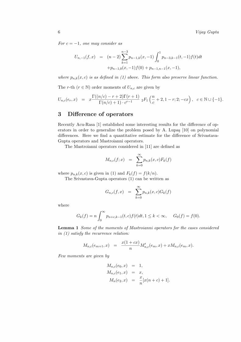
6 Vijay Gupta
For c = −1, one may consider as
Un,−1(f, x) = (n− 2)
n−3∑k=1
pn−1,k(x,−1)
∫ 1
0pn−3,k−1(t,−1)f(t)dt
+pn−1,0(x,−1)f(0) + pn−1,n−1(x,−1),
where pn,k(x, c) is as defined in (1) above. This form also preserve linear function.
The r-th (r ∈ N) order moments of Un,c are given by
Un,c(er, x) = xΓ((n/c)− r + 2)Γ(r + 1)
Γ(n/c) + 1) · cr−1 2F1
(nc
+ 2, 1− r; 2;−cx), c ∈ N ∪ {−1}.
3 Difference of operators
Recently Acu-Rasa [1] established some interesting results for the difference of op-erators in order to generalize the problem posed by A. Lupas [10] on polynomialdifferences. Here we find a quantitative estimate for the difference of Srivastava-Gupta operators and Mastroianni operators.
The Mastroianni operators considered in [11] are defined as
Mn,c(f ;x) =∞∑k=0
pn,k(x, c)Fk(f)
where pn,k(x, c) is given in (1) and Fk(f) = f(k/n).The Srivastava-Gupta operators (1) can be written as
Gn,c(f, x) =∞∑k=0
pn,k(x, c)Gk(f)
where
Gk(f) = n
∫ ∞0
pn+c,k−1(t, c)f(t)dt, 1 ≤ k <∞, G0(f) = f(0).
Lemma 1 Some of the moments of Mastroianni operators for the cases consideredin (1) satisfy the recurrence relation:
Mn,c(em+1, x) =x(1 + cx)
nM ′n,c(em, x) + xMn,c(em, x).
Few moments are given by
Mn,c(e0, x) = 1,
Mn,c(e1, x) = x,
Mn(e2, x) =x
n[x(n+ c) + 1].
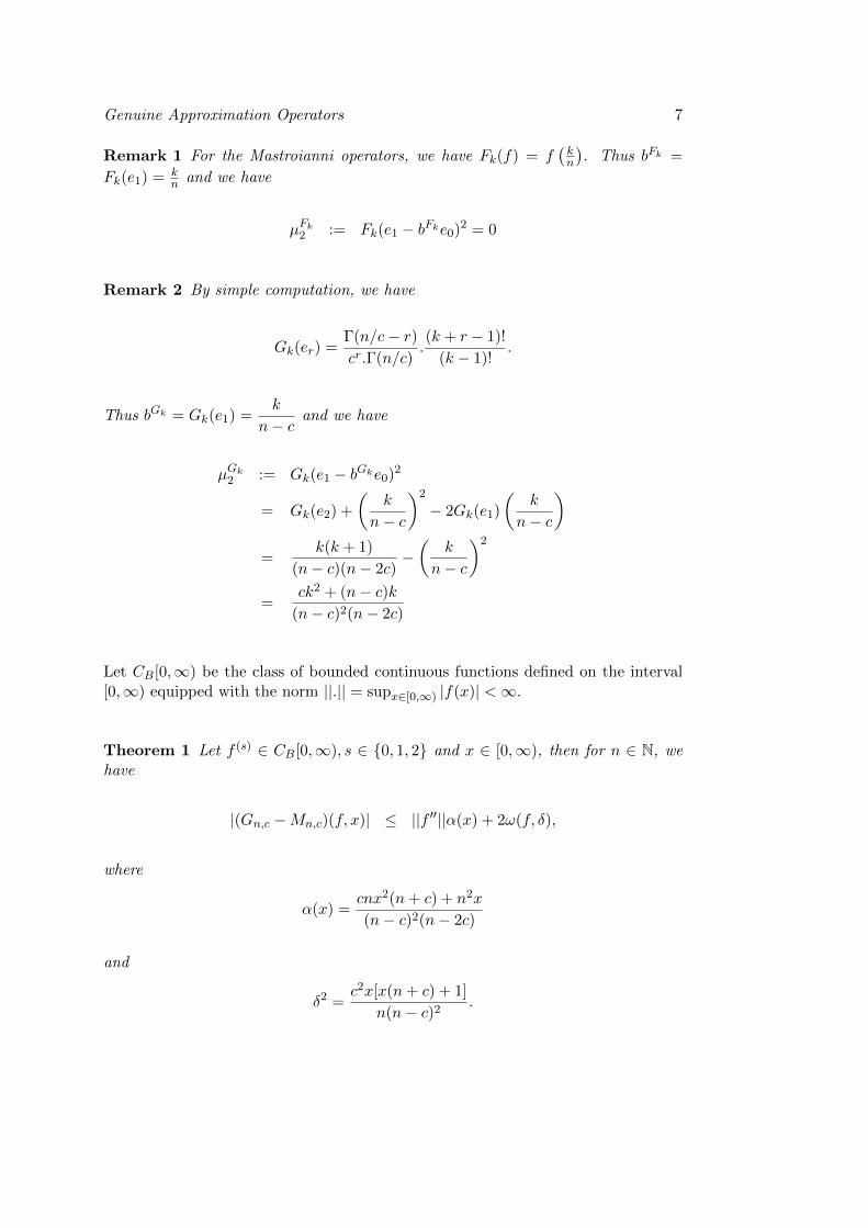
Genuine Approximation Operators 7
Remark 1 For the Mastroianni operators, we have Fk(f) = f(kn
). Thus bFk =
Fk(e1) = kn and we have
µFk2 := Fk(e1 − bFke0)
2 = 0
Remark 2 By simple computation, we have
Gk(er) =Γ(n/c− r)cr.Γ(n/c)
.(k + r − 1)!
(k − 1)!.
Thus bGk = Gk(e1) =k
n− cand we have
µGk2 := Gk(e1 − bGke0)
2
= Gk(e2) +
(k
n− c
)2
− 2Gk(e1)
(k
n− c
)=
k(k + 1)
(n− c)(n− 2c)−(
k
n− c
)2
=ck2 + (n− c)k
(n− c)2(n− 2c)
Let CB[0,∞) be the class of bounded continuous functions defined on the interval[0,∞) equipped with the norm ||.|| = supx∈[0,∞) |f(x)| <∞.
Theorem 1 Let f (s) ∈ CB[0,∞), s ∈ {0, 1, 2} and x ∈ [0,∞), then for n ∈ N, wehave
|(Gn,c −Mn,c)(f, x)| ≤ ||f ′′||α(x) + 2ω(f, δ),
where
α(x) =cnx2(n+ c) + n2x
(n− c)2(n− 2c)
and
δ2 =c2x[x(n+ c) + 1]
n(n− c)2.
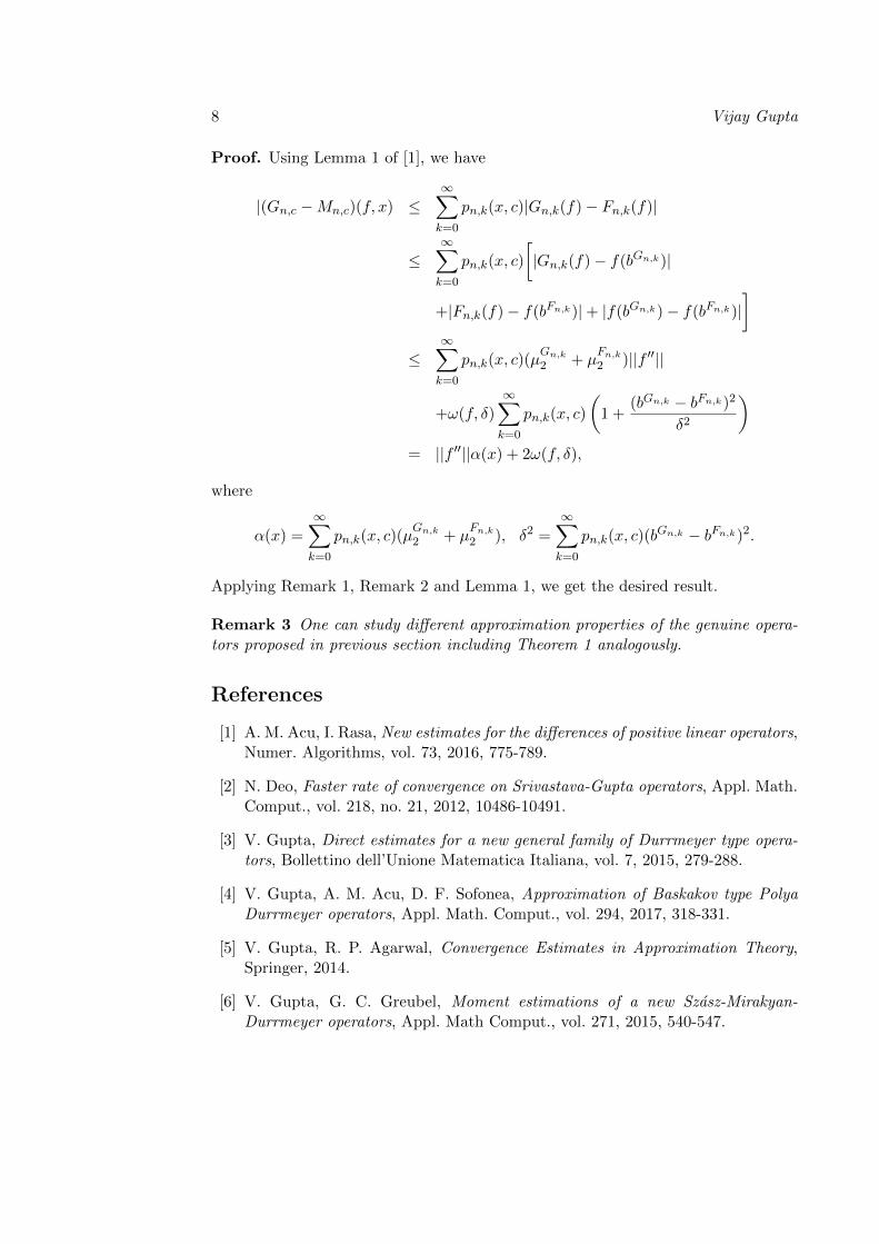
8 Vijay Gupta
Proof. Using Lemma 1 of [1], we have
|(Gn,c −Mn,c)(f, x) ≤∞∑k=0
pn,k(x, c)|Gn,k(f)− Fn,k(f)|
≤∞∑k=0
pn,k(x, c)
[|Gn,k(f)− f(bGn,k)|
+|Fn,k(f)− f(bFn,k)|+ |f(bGn,k)− f(bFn,k)|]
≤∞∑k=0
pn,k(x, c)(µGn,k
2 + µFn,k
2 )||f ′′||
+ω(f, δ)∞∑k=0
pn,k(x, c)
(1 +
(bGn,k − bFn,k)2
δ2
)= ||f ′′||α(x) + 2ω(f, δ),
where
α(x) =
∞∑k=0
pn,k(x, c)(µGn,k
2 + µFn,k
2 ), δ2 =
∞∑k=0
pn,k(x, c)(bGn,k − bFn,k)2.
Applying Remark 1, Remark 2 and Lemma 1, we get the desired result.
Remark 3 One can study different approximation properties of the genuine opera-tors proposed in previous section including Theorem 1 analogously.
References
[1] A. M. Acu, I. Rasa, New estimates for the differences of positive linear operators,Numer. Algorithms, vol. 73, 2016, 775-789.
[2] N. Deo, Faster rate of convergence on Srivastava-Gupta operators, Appl. Math.Comput., vol. 218, no. 21, 2012, 10486-10491.
[3] V. Gupta, Direct estimates for a new general family of Durrmeyer type opera-tors, Bollettino dell’Unione Matematica Italiana, vol. 7, 2015, 279-288.
[4] V. Gupta, A. M. Acu, D. F. Sofonea, Approximation of Baskakov type PolyaDurrmeyer operators, Appl. Math. Comput., vol. 294, 2017, 318-331.
[5] V. Gupta, R. P. Agarwal, Convergence Estimates in Approximation Theory,Springer, 2014.
[6] V. Gupta, G. C. Greubel, Moment estimations of a new Szasz-Mirakyan-Durrmeyer operators, Appl. Math Comput., vol. 271, 2015, 540-547.
Genuine Approximation Operators 9
[7] V. Gupta, G. Tachev, Approximation with Positive Linear Operators and LinearCombinations, Series: Developments in Mathematics, Springer, vol. 50, 2017.
[8] V. Gupta, R. Yadav, On the approximation of certain integral operators, ActaMath Vietnamica, vol. 39, 2014, 193-203.
[9] N. Ispir, I. Yuksel, On the Bezier variant of Srivastava-Gupta operators, Appl.Math E Notes, vol. 5, 2005, 129-137.
[10] A. Lupas, The approximation by means of some linear positive operators, In:Approximation Theory (M.W. Muller others, eds), Akademie-Verlag, Berlin,1995, 201-227.
[11] Antonio-Jess Lpez-Moreno, Jos-Manuel, Latorre-Palacios, Localization resultsfor generalized Baskakov/Mastroianni and composite operators, J. Math. Anal.Appl., vol. 380, no. 2, 2011, 425-439.
[12] H. M. Srivastava, V. Gupta, A certain family of summation-integral type oper-ators, Math. Comput. Modelling, vol. 37, 2003, 1307-1315.
[13] D. K. Verma, P. N. Agrawal, Convergence in simultaneous approxima-tion for Srivastava-Gupta operators, Math. Sci., vol. 22, no. 6, 2012,https://doi.org/10.1186/2251-7456-6-22.
Vijay GuptaNetaji Subhas University of TechnologyDepartment of MathematicsSector 3 Dwarka, New Delhi 110078e-mail: [email protected]

General Mathematics Vol. 26, No. 1-2 (2018), 11–23
Applications of Fractional Calculus for a CertainSubclass of Multivalent Analytic Functions on
Complex Hilbert Space 1
Abbas Kareem Wanas, B. A. Frasin
Abstract
The object of the present paper is to study an applications of the
fractional integral and the fractional derivative techniques for a certain
subclass of multivalent analytic functions on Hilbert space and obtain
some important geometric properties such as coefficient estimates, ex-
treme points and convex combination.
2010 Mathematics Subject Classification: 30C45,30C50.
Key words and phrases: Multivalent functions, Fractional calculus,
Convex combination, Hilbert space.
1 Introduction
Let A(p,m) denote the class of functions of the form:
(1) f(z) = zp +
∞∑n=p+m
anzn (p,m ∈ N = {1, 2, · · · }),
which are analytic and multivalent in the open unit disk U = {z ∈ C : |z| < 1}.1Received 15 May , 2018
Accepted for publication (in revised form) 2 August, 2018
11
12 Abbas Kareem Wanas, B. A. Frasin
Let F (p,m) denote the subclass of A(p,m) consisting of functions of the
form:
(2) f(z) = zp −∞∑
n=p+m
anzn (an ≥ 0, p,m ∈ N = {1, 2, · · · }).
A function f ∈ A(p,m) is said to be multivalent starlike of order α(0 ≤α < p) if it satisfies the condition:
Re
{zf ′(z)
f(z)
}> α (z ∈ U),
and is said to be multivalent convex of order α(0 ≤ α < p) if it satisfies the
condition:
Re
{1 +
zf ′′(z)
f ′(z)
}> α (z ∈ U).
Denote by S∗m(p, α) and Cm(p, α) the classes of multivalent starlike and mul-
tivalent convex functions of order α, respectively, which were introduced and
studied by Owa [12]. It is known that (see [7] and [12])
f ∈ Cm(p, α) if and only iff ′(z)
p∈ S∗m(p, α).
The classes S∗1(p, α) = S∗(p, α) and C1(p, α) = C(p, α) were studied by Own
[11].
Let H be a complex Hilbert space. Let T be a linear operator on H. For a
complex analytic function f on the unit disk U , we denoted f(T ), the operator
on H defined by the usual Riesz-Dunford integral [2]
f(T ) =1
2πi
∫cf(z) (zI − T )−1 dz,
where I is the identity operator on H, c is a positively oriented simple closed
rectifiable contour lying in U and containing the spectrum σ(T ) of T in its
interior domain [3]. Also f(T ) can be defined by the series
f(T ) =∞∑n=0
f (n)(0)
n!Tn,
which converges in the norm topology [4].
Applications of Fractional Calculus for a Certain Subclass 13
Definition 1 [13]. The fractional integral operator of order λ(λ > 0) is de-
fined by
D−λT f(T ) =1
Γ(λ)
∫ 1
0
T λf(tT )
(1− t)1−λdt,
where f is analytic function in a simply connected region of z-plane containing
the origin.
Definition 2 [13]. The fractional derivative for operator of order λ(0 ≤ λ <1) is defined by
DλT f(T ) =
1
Γ(1− λ)
d
dT
∫ 1
0
T 1−λf(tT )
(1− t)λdt,
where f is analytic in a simply connected region of z-plane containing the
origin.
For f ∈ F (p,m), from Definition 1 and Definition 2, we get
(3) D−λT f(T ) =Γ(p+ 1)
Γ(p+ λ+ 1)T p+λ −
∞∑n=p+m
Γ(n+ 1)
Γ(n+ λ+ 1)anT
n+λ
and
(4) DλT f(T ) =
Γ(p+ 1)
Γ(p− λ+ 1)T p−λ −
∞∑n=p+m
Γ(n+ 1)
Γ(n− λ+ 1)anT
n−λ
Definition 3 A function f ∈ F (p,m) is said to be in the class AF (p,m, γ, δ, τ, T )
if and only if satisfies the inequality:
(5)∥∥Tf ′′′(T )− (p− 2)f ′′(T )
∥∥ < ∥∥γTf ′′′(T ) + (δ − τ)f ′′(T )∥∥ ,
where 0 ≤ γ < 1, 0 < δ ≤ 1, 0 ≤ τ < 1, p,m ∈ N, p > 2 and for all operator
T with ‖T‖ < 1 and T 6= ∅ (∅ denote the zero operator on H).
The operators on Hilbert space were considered recently be Xiaopei [15],
Joshi [8], Chrauim et al. [1], Ghanim and Darus [6], selvaraj et al. [13],
Murugusundaramoorthy et al. [10], Gbolagade and Makinde [5], Joshi et al.
[9] and Wanas and Jebur [14].
14 Abbas Kareem Wanas, B. A. Frasin
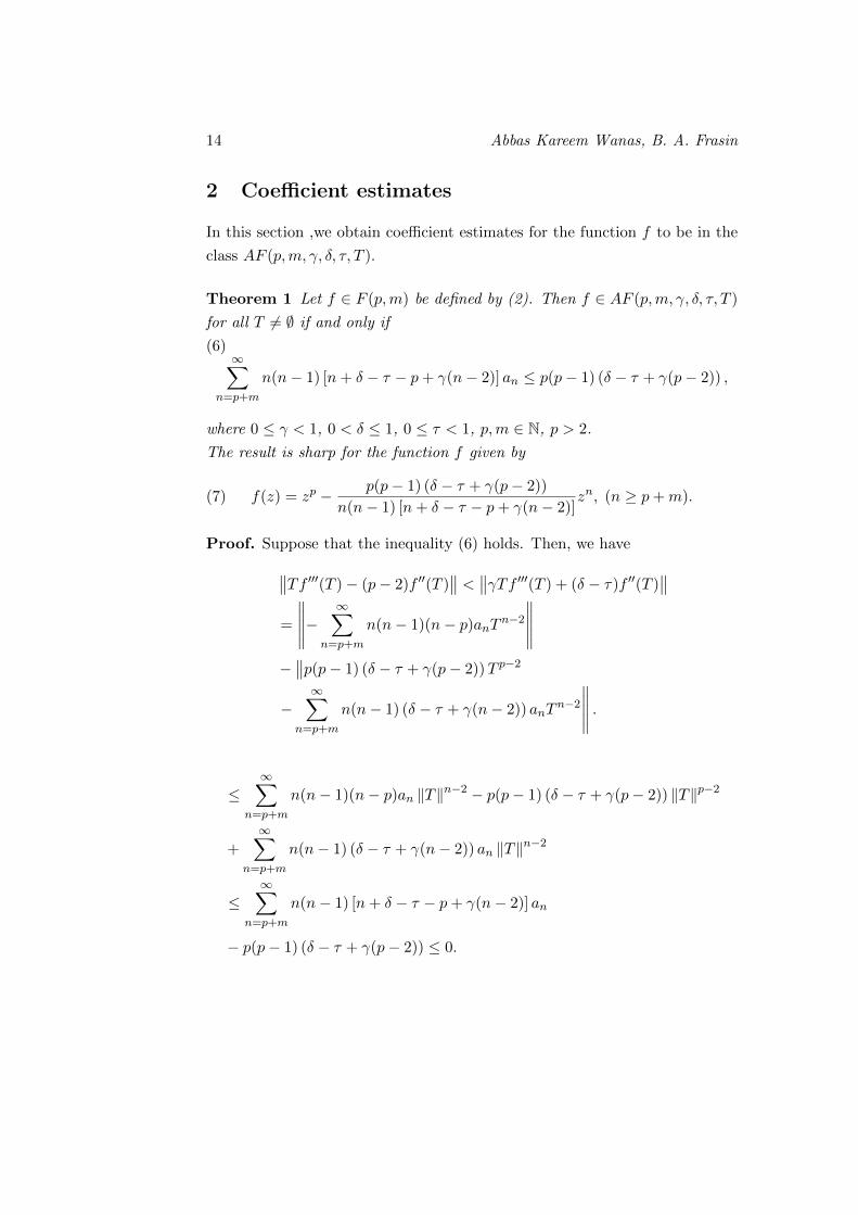
2 Coefficient estimates
In this section ,we obtain coefficient estimates for the function f to be in the
class AF (p,m, γ, δ, τ, T ).
Theorem 1 Let f ∈ F (p,m) be defined by (2). Then f ∈ AF (p,m, γ, δ, τ, T )
for all T 6= ∅ if and only if
(6)∞∑
n=p+m
n(n− 1) [n+ δ − τ − p+ γ(n− 2)] an ≤ p(p− 1) (δ − τ + γ(p− 2)) ,
where 0 ≤ γ < 1, 0 < δ ≤ 1, 0 ≤ τ < 1, p,m ∈ N, p > 2.
The result is sharp for the function f given by
(7) f(z) = zp − p(p− 1) (δ − τ + γ(p− 2))
n(n− 1) [n+ δ − τ − p+ γ(n− 2)]zn, (n ≥ p+m).
Proof. Suppose that the inequality (6) holds. Then, we have∥∥Tf ′′′(T )− (p− 2)f ′′(T )∥∥ < ∥∥γTf ′′′(T ) + (δ − τ)f ′′(T )
∥∥=
∥∥∥∥∥−∞∑
n=p+m
n(n− 1)(n− p)anTn−2∥∥∥∥∥
−∥∥p(p− 1) (δ − τ + γ(p− 2))T p−2
−∞∑
n=p+m
n(n− 1) (δ − τ + γ(n− 2)) anTn−2
∥∥∥∥∥ .
≤∞∑
n=p+m
n(n− 1)(n− p)an ‖T‖n−2 − p(p− 1) (δ − τ + γ(p− 2)) ‖T‖p−2
+∞∑
n=p+m
n(n− 1) (δ − τ + γ(n− 2)) an ‖T‖n−2
≤∞∑
n=p+m
n(n− 1) [n+ δ − τ − p+ γ(n− 2)] an
− p(p− 1) (δ − τ + γ(p− 2)) ≤ 0.
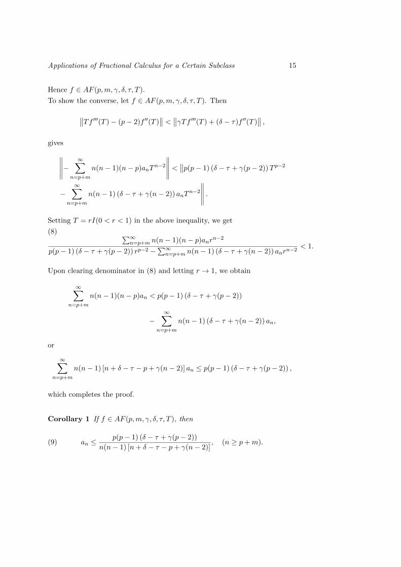
Applications of Fractional Calculus for a Certain Subclass 15
Hence f ∈ AF (p,m, γ, δ, τ, T ).
To show the converse, let f ∈ AF (p,m, γ, δ, τ, T ). Then
∥∥Tf ′′′(T )− (p− 2)f ′′(T )∥∥ < ∥∥γTf ′′′(T ) + (δ − τ)f ′′(T )
∥∥ ,gives∥∥∥∥∥−
∞∑n=p+m
n(n− 1)(n− p)anTn−2∥∥∥∥∥ < ∥∥p(p− 1) (δ − τ + γ(p− 2))T p−2
−∞∑
n=p+m
n(n− 1) (δ − τ + γ(n− 2)) anTn−2
∥∥∥∥∥ .Setting T = rI(0 < r < 1) in the above inequality, we get
(8) ∑∞n=p+m n(n− 1)(n− p)anrn−2
p(p− 1) (δ − τ + γ(p− 2)) rp−2 −∑∞
n=p+m n(n− 1) (δ − τ + γ(n− 2)) anrn−2< 1.
Upon clearing denominator in (8) and letting r → 1, we obtain
∞∑n=p+m
n(n− 1)(n− p)an < p(p− 1) (δ − τ + γ(p− 2))
−∞∑
n=p+m
n(n− 1) (δ − τ + γ(n− 2)) an,
or
∞∑n=p+m
n(n− 1) [n+ δ − τ − p+ γ(n− 2)] an ≤ p(p− 1) (δ − τ + γ(p− 2)) ,
which completes the proof.
Corollary 1 If f ∈ AF (p,m, γ, δ, τ, T ), then
(9) an ≤p(p− 1) (δ − τ + γ(p− 2))
n(n− 1) [n+ δ − τ − p+ γ(n− 2)], (n ≥ p+m).
16 Abbas Kareem Wanas, B. A. Frasin
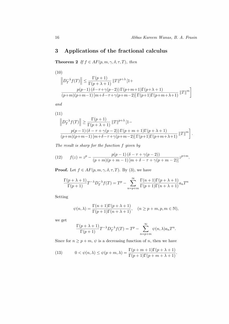
3 Applications of the fractional calculus
Theorem 2 If f ∈ AF (p,m, γ, δ, τ, T ), then
∥∥∥D−λT f(T )∥∥∥ ≤ Γ(p+ 1)
Γ(p+ λ+ 1)‖T‖p+λ [1+
(10)
p(p−1) (δ−τ+γ(p−2)) Γ(p+m+1)Γ(p+λ+ 1)
(p+m)(p+m−1) [m+δ−τ+γ(p+m−2)] Γ(p+1)Γ(p+m+λ+1)‖T‖m
]and
∥∥∥D−λT f(T )∥∥∥ ≥ Γ(p+ 1)
Γ(p+ λ+ 1)‖T‖p+λ [1−
(11)
p(p− 1) (δ − τ + γ(p− 2)) Γ(p+m+ 1)Γ(p+ λ+ 1)
(p+m)(p+m−1) [m+δ−τ+γ(p+m−2)] Γ(p+1)Γ(p+m+λ+1)‖T‖m
].
The result is sharp for the function f given by
(12) f(z) = zp − p(p− 1) (δ − τ + γ(p− 2))
(p+m)(p+m− 1) [m+ δ − τ + γ(p+m− 2)]zp+m.
Proof. Let f ∈ AF (p,m, γ, δ, τ, T ). By (3), we have
Γ(p+ λ+ 1)
Γ(p+ 1)T−λD−λT f(T ) = T p −
∞∑n=p+m
Γ(n+ 1)Γ(p+ λ+ 1)
Γ(p+ 1)Γ(n+ λ+ 1)anT
n
Setting
ψ(n, λ) =Γ(n+ 1)Γ(p+ λ+ 1)
Γ(p+ 1)Γ(n+ λ+ 1), (n ≥ p+m, p,m ∈ N),
we get
Γ(p+ λ+ 1)
Γ(p+ 1)T−λD−λT f(T ) = T p −
∞∑n=p+m
ψ(n, λ)anTn.
Since for n ≥ p+m, ψ is a decreasing function of n, then we have
(13) 0 < ψ(n, λ) ≤ ψ(p+m,λ) =Γ(p+m+ 1)Γ(p+ λ+ 1)
Γ(p+ 1)Γ(p+m+ λ+ 1).
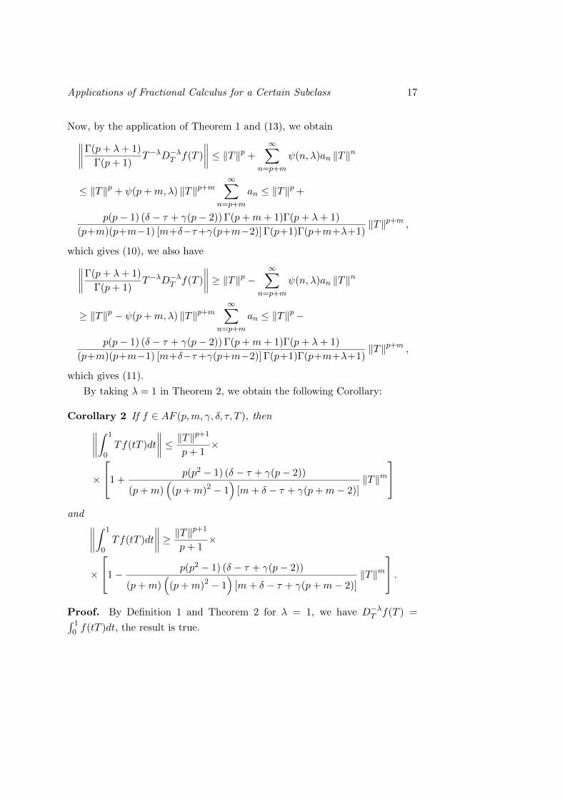
Applications of Fractional Calculus for a Certain Subclass 17
Now, by the application of Theorem 1 and (13), we obtain∥∥∥∥Γ(p+ λ+ 1)
Γ(p+ 1)T−λD−λT f(T )
∥∥∥∥ ≤ ‖T‖p +∞∑
n=p+m
ψ(n, λ)an ‖T‖n
≤ ‖T‖p + ψ(p+m,λ) ‖T‖p+m∞∑
n=p+m
an ≤ ‖T‖p +
p(p− 1) (δ − τ + γ(p− 2)) Γ(p+m+ 1)Γ(p+ λ+ 1)
(p+m)(p+m−1) [m+δ−τ+γ(p+m−2)] Γ(p+1)Γ(p+m+λ+1)‖T‖p+m ,
which gives (10), we also have∥∥∥∥Γ(p+ λ+ 1)
Γ(p+ 1)T−λD−λT f(T )
∥∥∥∥ ≥ ‖T‖p − ∞∑n=p+m
ψ(n, λ)an ‖T‖n
≥ ‖T‖p − ψ(p+m,λ) ‖T‖p+m∞∑
n=p+m
an ≤ ‖T‖p−
p(p− 1) (δ − τ + γ(p− 2)) Γ(p+m+ 1)Γ(p+ λ+ 1)
(p+m)(p+m−1) [m+δ−τ+γ(p+m−2)] Γ(p+1)Γ(p+m+λ+1)‖T‖p+m ,
which gives (11).
By taking λ = 1 in Theorem 2, we obtain the following Corollary:
Corollary 2 If f ∈ AF (p,m, γ, δ, τ, T ), then∥∥∥∥∫ 1
0Tf(tT )dt
∥∥∥∥ ≤ ‖T‖p+1
p+ 1×
×
1 +p(p2 − 1) (δ − τ + γ(p− 2))
(p+m)(
(p+m)2 − 1)
[m+ δ − τ + γ(p+m− 2)]‖T‖m
and ∥∥∥∥∫ 1
0Tf(tT )dt
∥∥∥∥ ≥ ‖T‖p+1
p+ 1×
×
1− p(p2 − 1) (δ − τ + γ(p− 2))
(p+m)(
(p+m)2 − 1)
[m+ δ − τ + γ(p+m− 2)]‖T‖m
.Proof. By Definition 1 and Theorem 2 for λ = 1, we have D−λT f(T ) =∫ 10 f(tT )dt, the result is true.
18 Abbas Kareem Wanas, B. A. Frasin
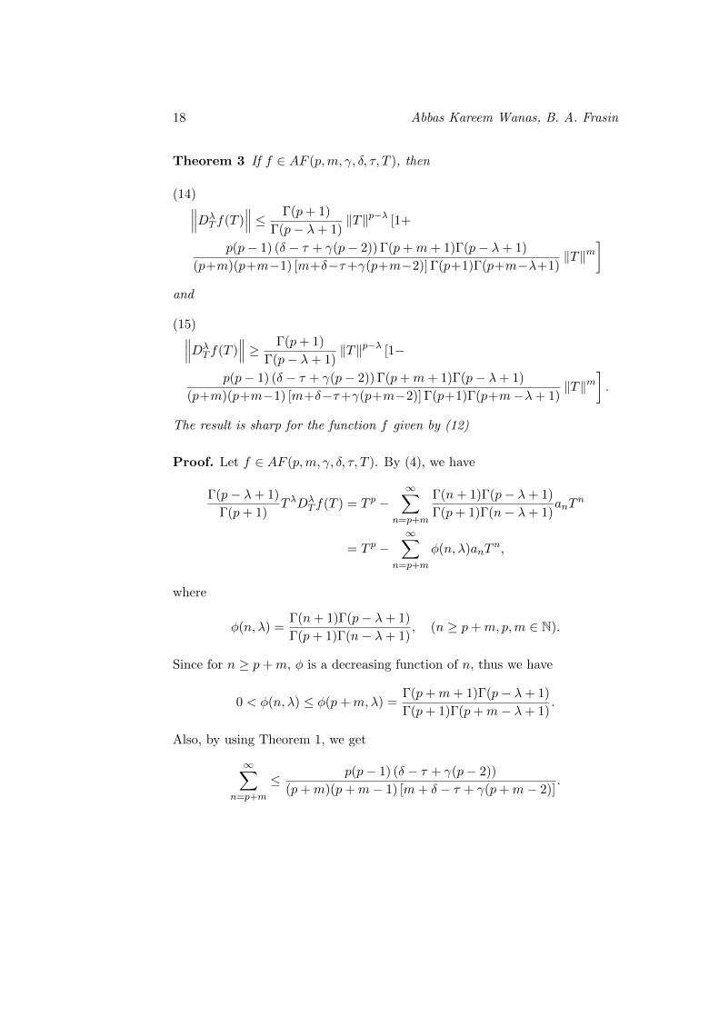
Theorem 3 If f ∈ AF (p,m, γ, δ, τ, T ), then
∥∥∥DλT f(T )
∥∥∥ ≤ Γ(p+ 1)
Γ(p− λ+ 1)‖T‖p−λ [1+
(14)
p(p− 1) (δ − τ + γ(p− 2)) Γ(p+m+ 1)Γ(p− λ+ 1)
(p+m)(p+m−1) [m+δ−τ+γ(p+m−2)] Γ(p+1)Γ(p+m−λ+1)‖T‖m
]and
∥∥∥DλT f(T )
∥∥∥ ≥ Γ(p+ 1)
Γ(p− λ+ 1)‖T‖p−λ [1−
(15)
p(p− 1) (δ − τ + γ(p− 2)) Γ(p+m+ 1)Γ(p− λ+ 1)
(p+m)(p+m−1) [m+δ−τ+γ(p+m−2)] Γ(p+1)Γ(p+m−λ+ 1)‖T‖m
].
The result is sharp for the function f given by (12)
Proof. Let f ∈ AF (p,m, γ, δ, τ, T ). By (4), we have
Γ(p− λ+ 1)
Γ(p+ 1)T λDλ
T f(T ) = T p −∞∑
n=p+m
Γ(n+ 1)Γ(p− λ+ 1)
Γ(p+ 1)Γ(n− λ+ 1)anT
n
= T p −∞∑
n=p+m
φ(n, λ)anTn,
where
φ(n, λ) =Γ(n+ 1)Γ(p− λ+ 1)
Γ(p+ 1)Γ(n− λ+ 1), (n ≥ p+m, p,m ∈ N).
Since for n ≥ p+m, φ is a decreasing function of n, thus we have
0 < φ(n, λ) ≤ φ(p+m,λ) =Γ(p+m+ 1)Γ(p− λ+ 1)
Γ(p+ 1)Γ(p+m− λ+ 1).
Also, by using Theorem 1, we get
∞∑n=p+m
≤ p(p− 1) (δ − τ + γ(p− 2))
(p+m)(p+m− 1) [m+ δ − τ + γ(p+m− 2)].
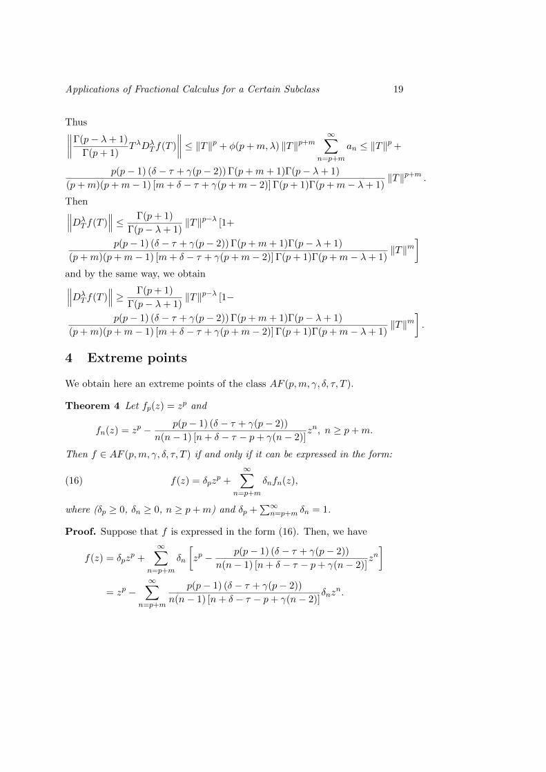
Applications of Fractional Calculus for a Certain Subclass 19
Thus∥∥∥∥Γ(p− λ+ 1)
Γ(p+ 1)T λDλ
T f(T )
∥∥∥∥ ≤ ‖T‖p + φ(p+m,λ) ‖T‖p+m∞∑
n=p+m
an ≤ ‖T‖p +
p(p− 1) (δ − τ + γ(p− 2)) Γ(p+m+ 1)Γ(p− λ+ 1)
(p+m)(p+m− 1) [m+ δ − τ + γ(p+m− 2)] Γ(p+ 1)Γ(p+m− λ+ 1)‖T‖p+m .
Then∥∥∥DλT f(T )
∥∥∥ ≤ Γ(p+ 1)
Γ(p− λ+ 1)‖T‖p−λ [1+
p(p− 1) (δ − τ + γ(p− 2)) Γ(p+m+ 1)Γ(p− λ+ 1)
(p+m)(p+m− 1) [m+ δ − τ + γ(p+m− 2)] Γ(p+ 1)Γ(p+m− λ+ 1)‖T‖m
]and by the same way, we obtain∥∥∥Dλ
T f(T )∥∥∥ ≥ Γ(p+ 1)
Γ(p− λ+ 1)‖T‖p−λ [1−
p(p− 1) (δ − τ + γ(p− 2)) Γ(p+m+ 1)Γ(p− λ+ 1)
(p+m)(p+m− 1) [m+ δ − τ + γ(p+m− 2)] Γ(p+ 1)Γ(p+m− λ+ 1)‖T‖m
].
4 Extreme points
We obtain here an extreme points of the class AF (p,m, γ, δ, τ, T ).
Theorem 4 Let fp(z) = zp and
fn(z) = zp − p(p− 1) (δ − τ + γ(p− 2))
n(n− 1) [n+ δ − τ − p+ γ(n− 2)]zn, n ≥ p+m.
Then f ∈ AF (p,m, γ, δ, τ, T ) if and only if it can be expressed in the form:
(16) f(z) = δpzp +
∞∑n=p+m
δnfn(z),
where (δp ≥ 0, δn ≥ 0, n ≥ p+m) and δp +∑∞
n=p+m δn = 1.
Proof. Suppose that f is expressed in the form (16). Then, we have
f(z) = δpzp +
∞∑n=p+m
δn
[zp − p(p− 1) (δ − τ + γ(p− 2))
n(n− 1) [n+ δ − τ − p+ γ(n− 2)]zn]
= zp −∞∑
n=p+m
p(p− 1) (δ − τ + γ(p− 2))
n(n− 1) [n+ δ − τ − p+ γ(n− 2)]δnz
n.
20 Abbas Kareem Wanas, B. A. Frasin
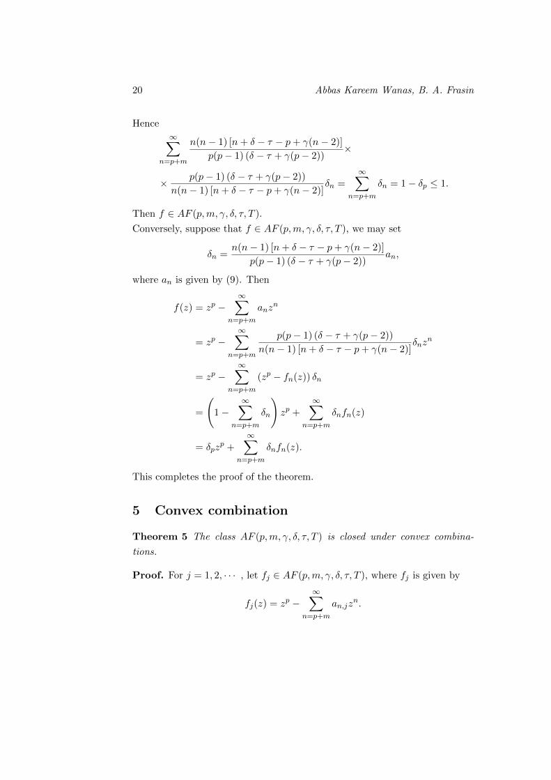
Hence
∞∑n=p+m
n(n− 1) [n+ δ − τ − p+ γ(n− 2)]
p(p− 1) (δ − τ + γ(p− 2))×
× p(p− 1) (δ − τ + γ(p− 2))
n(n− 1) [n+ δ − τ − p+ γ(n− 2)]δn =
∞∑n=p+m
δn = 1− δp ≤ 1.
Then f ∈ AF (p,m, γ, δ, τ, T ).
Conversely, suppose that f ∈ AF (p,m, γ, δ, τ, T ), we may set
δn =n(n− 1) [n+ δ − τ − p+ γ(n− 2)]
p(p− 1) (δ − τ + γ(p− 2))an,
where an is given by (9). Then
f(z) = zp −∞∑
n=p+m
anzn
= zp −∞∑
n=p+m
p(p− 1) (δ − τ + γ(p− 2))
n(n− 1) [n+ δ − τ − p+ γ(n− 2)]δnz
n
= zp −∞∑
n=p+m
(zp − fn(z)) δn
=
(1−
∞∑n=p+m
δn
)zp +
∞∑n=p+m
δnfn(z)
= δpzp +
∞∑n=p+m
δnfn(z).
This completes the proof of the theorem.
5 Convex combination
Theorem 5 The class AF (p,m, γ, δ, τ, T ) is closed under convex combina-
tions.
Proof. For j = 1, 2, · · · , let fj ∈ AF (p,m, γ, δ, τ, T ), where fj is given by
fj(z) = zp −∞∑
n=p+m
an,jzn.
Applications of Fractional Calculus for a Certain Subclass 21
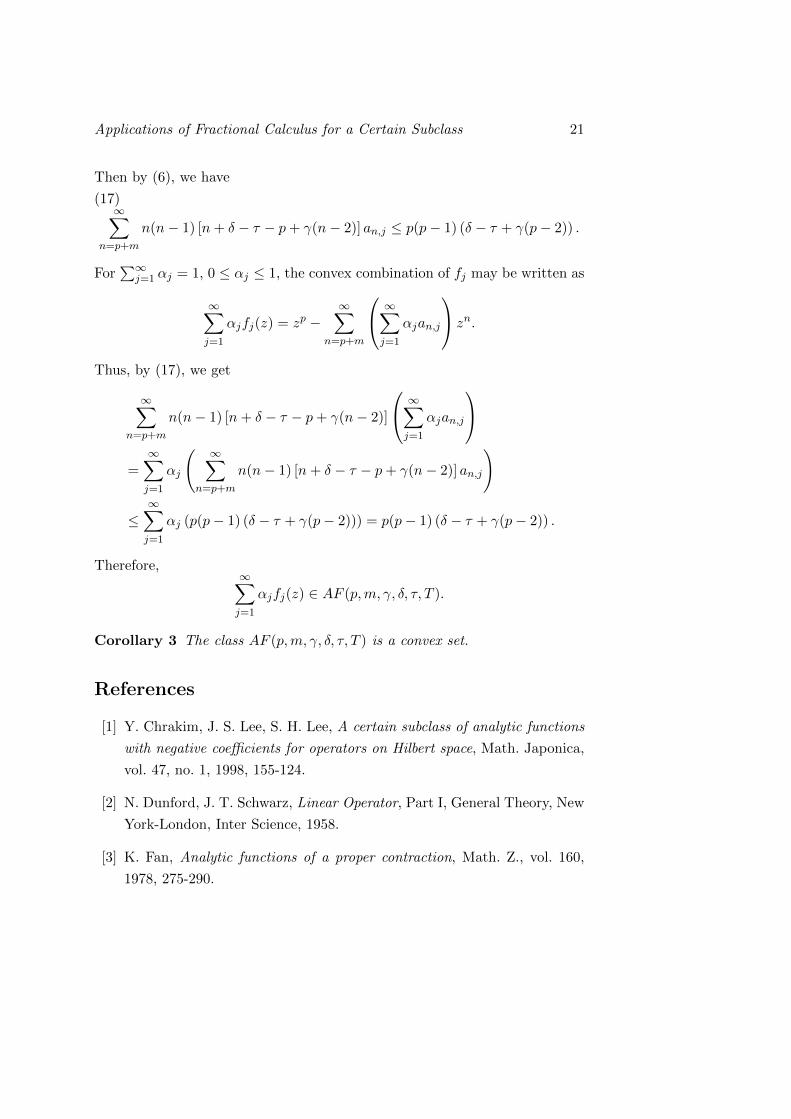
Then by (6), we have
(17)∞∑
n=p+m
n(n− 1) [n+ δ − τ − p+ γ(n− 2)] an,j ≤ p(p− 1) (δ − τ + γ(p− 2)) .
For∑∞
j=1 αj = 1, 0 ≤ αj ≤ 1, the convex combination of fj may be written as
∞∑j=1
αjfj(z) = zp −∞∑
n=p+m
∞∑j=1
αjan,j
zn.
Thus, by (17), we get
∞∑n=p+m
n(n− 1) [n+ δ − τ − p+ γ(n− 2)]
∞∑j=1
αjan,j
=∞∑j=1
αj
( ∞∑n=p+m
n(n− 1) [n+ δ − τ − p+ γ(n− 2)] an,j
)
≤∞∑j=1
αj (p(p− 1) (δ − τ + γ(p− 2))) = p(p− 1) (δ − τ + γ(p− 2)) .
Therefore,∞∑j=1
αjfj(z) ∈ AF (p,m, γ, δ, τ, T ).
Corollary 3 The class AF (p,m, γ, δ, τ, T ) is a convex set.
References
[1] Y. Chrakim, J. S. Lee, S. H. Lee, A certain subclass of analytic functions
with negative coefficients for operators on Hilbert space, Math. Japonica,
vol. 47, no. 1, 1998, 155-124.
[2] N. Dunford, J. T. Schwarz, Linear Operator, Part I, General Theory, New
York-London, Inter Science, 1958.
[3] K. Fan, Analytic functions of a proper contraction, Math. Z., vol. 160,
1978, 275-290.
22 Abbas Kareem Wanas, B. A. Frasin
[4] K. Fan, Julias lemma for operators, Math. Ann., vol. 239, 1979, 241-245.
[5] A. M. Gbolagade, D. O. Makinde, Operator on Hilbert space and its ap-
plication to certain multivalent functions with fixed point associated with
hypergeometric function, Tbilisi Math. J., vol. 9, no. 2, 2016, 151-157.
[6] F. Ghanim, M. Darus, On new subclass of analytic p-valent function with
negative coefficients for operators on Hilbert space, Int. Math. Forum, vol.
3, no. 2, 2008, 69-77.
[7] A. W. Goodman, Univalent Functions, Vols. I and II, Palygonal House,
Washington, New Jersey, 1983.
[8] S. B. Joshi, On a class of analytic functions with negative coefficients for
operators on Hilbert Space, J. Appr. Theory and Appl., 1998, 107-112.
[9] S. Joshi, S. B. Joshi, R. Mohapatra, On a subclass of analytic functions
for operator on a Hilbert space, Stud. Univ. Babes-Bolyai Math., vol. 61,
no. 2, 2016, 147-153.
[10] G. Murugusundaramoorthy, K. Uma, M. Darus, Analytic functions as-
sociated with Caputos fractional differentiation defined by Hilbert space
operator, Boletin de la Asociacion Matematica Venezolana, vol. XVIII,
no. 2, 2011, 111-125.
[11] S. Owa, On certain classes of p-valent functions with negative coefficients,
Siman Stevin, vol. 59, 1985, 385-402.
[12] S. Owa, The quasi-Hadamard products of certion analytic functions, in
Current Topics in Analytic Function Theory, H. M. Srivastava and Owa,
(Editors), World Scientific Publishing Company , Singapore, New Jersey,
London, and Hong Kony, 1992, 234-251.
[13] C. Selvaraj, A. J. Pamela, M. Thirucheran, On a subclass of multivalent
analytic functions with negative coefficients for contraction operators on
Hilbert space, Int. J. Contemp. Math. Sci., vol. 4, no. 9, 2009, 447-456.
Applications of Fractional Calculus for a Certain Subclass 23
[14] A. K. Wanas, S. K. Jebur, Geometric Properties for a family of p-valent
holomorphic functions with negative coefficients for operator on Hilbert
space, Journal of AL-Qadisiyah for Computer Science and Mathematics,
vol. 10, no. 2, 2018, 1-5.
[15] Y. Xiapei, A subclass of analytic p-valent functions for operator on Hilbert
space, Math. Japonica, vol. 40, no. 2, 1994, 303-308.
Abbas Kareem Wanas
University of Al-Qadisiyah
College of Science
Department of Mathematics
Diwaniya, Iraq
e-mail: [email protected]
B. A. Frasin
Al al-Bayt University
Faculty of Science
Department of Mathematics
Mafraq, Jordan
e-mail: [email protected]

General Mathematics Vol. 26, No. 1-2 (2018), 25–34
Some Classes Of Multivalent Starlike Functions WithRespect To Symmetric Conjugate Points 1
K. R. Karthikeyan, K. Srinivasan, K. Ramachandran
Abstract
A new subclass of multivalent analytic functions with respect to conjugatesymmetric functions are introduced. Relationship with other well known classessuch as convex and starlike functions have been established. Further, veryinteresting conditions for starlikeness have been obtained using subordination.
2010 Mathematics Subject Classification: 30C45
Key words and phrases: multivalent, starlike, convex, (j, k)- symmetricalfunctions, differential subordination.
1 Introduction
Let U = {z ∈ C : | z |< 1} be the open unit disc. Let H be the class of functionsanalytic in U . Let H(a, n) be the subclass of H consisting of functions of the formf(z) = a+ anz
n + an+1zn+1 + · · · .
Let Ap denote the class of all analytic functions of the form
(1) f(z) = zp +∞∑
k=p+1
akzk (p ∈ N := {1, 2, 3, . . . }) ,
and let A = A1.
Let the functions f(z) and g(z) be members of A. We say that the functionf is subordinate to g (or g is superordinate to f), written f ≺ g, if there existsa Schwarz function w analytic in U , with w(0) = 0 and |w(z)| < 1 and such thatf(z) = g(w(z)). In particular, if g is univalent, then f ≺ g if and only if f(0) = g(0)and f(U) ⊂ g(U).
1Received 19 May, 2016Accepted for publication (in revised form) 11 May, 2018
25
26 K. R. Karthikeyan, K. Srinivasan, K. Ramachandran
We denote by S∗, C, K and C∗ the familiar subclasses of A consisting of functionswhich are respectively starlike, convex, close-to-convex and quasi-convex in U . Also,we let P to denote the class of functions analytic in U having Taylor series expansionof the form
h(z) = 1 +∞∑n=1
hnzn,
and satisfy the condition Re {h(z)} > 0, (z ∈ U). Our favorite references of the fieldare [3, 4] which covers most of the topics in a lucid and economical style.
Motivated by the concept introduced by K. Sakaguchi in [9], recently severalsubclasses of analytic functions with respect to k-symmetric points were introducedand studied by various authors. More prominently, Wang et. al. in [11] introduced
class S(k)s
(ϕ)
of functions f ∈ A subject to satisfying the condition
zf ′(z)
fk(z)≺ ϕ(z) (z ∈ U) ,
where ϕ(z) ∈ P, k ≥ 1 is fixed positive integer and fk(z) is defined by the equality
fj, k(z) =1
k
k−1∑ν=0
ενf(ενz).
Similarly, C(k)s
(ϕ)
denote the class of functions in S satisfying the condition
(zf ′(z))′
f ′k(z)≺ ϕ(z) (z ∈ U) ,
where ϕ(z) ∈ P, k ≥ 1 is fixed positive integerLiczberski and Po lubinski in [6] introduced the notion (j, k) symmetrical function
(k = 2, 3, . . . ; j = 0, 1, . . . , k − 1), which is a generalization of even, odd and k-symmetrical functions. A function f ∈ A is said to be (j, k)-symmetrical if for eachz ∈ U
(2) f(εz) = εjf(z),
(k = 1, 2, . . . ; j = 0, 1, 2, . . . (k − 1)),
where ε = exp(2πi/k). The family of (j, k)-symmetrical functions will be denotedby F jk . We observe that F1
2 , F02 and F1
k are well-known families of odd functions,even functions and k-symmetrical functions respectively. It was further proved in[6] that each function defined on a symmetrical set can be uniquely represented asthe sum of an even function and an odd function.
Also let fj, k(z) be defined by the following equality
(3) fj, k(z) =1
k
k−1∑ν=0
f(ενz)
ενpj,
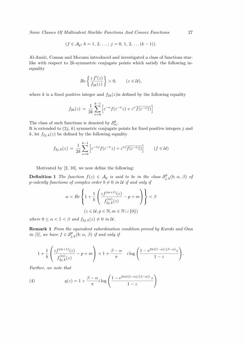
Some Classes Of Multivalent Starlike Functions And Convex Functions 27
(f ∈ Ap; k = 1, 2, . . . ; j = 0, 1, 2, . . . (k − 1)).
Al-Amiri, Coman and Mocanu introduced and investigated a class of functions star-like with respect to 2k-symmetric conjugate points which satisfy the following in-equality
Re
{z f ′(z)
f2k(z)
}> 0, (z ∈ U),
where k is a fixed positive integer and f2k(z)is defined by the following equality
f2k(z) =1
2k
k−1∑ν=0
[ε−νf(ε−νz) + ενf(ε−νz)
]The class of such functions is denoted by Sksc.It is extended to (2j, k) symmetric conjugate points for fixed positive integers j andk, let f2j, k(z) be defined by the following equality
f2j, k(z) =1
2k
k−1∑ν=0
[ε−νjf(ε−νz) + ενjf(ε−νz)
](f ∈ U)
Motivated by [2, 10], we now define the following:
Definition 1 The function f(z) ∈ Ap is said to be in the class Spj, k(b; α, β) ofp-valently functions of complex order b 6= 0 in U if and only if
α < Re
1 +1
b
zf (m+1)(z)
f(m)2j, k(z)
− p+m
< β
(z ∈ U , p ∈ N,m ∈ N ∪ {0})
where 0 ≤ α < 1 < β and f2j, k(z) 6= 0 in U .
Remark 1 From the equivalent subordination condition proved by Kuroki and Owain [5], we have f ∈ Spj, k(b; α, β) if and only if
1 +1
b
zf (m+1)(z)
f(m)2j, k(z)
− p+m
≺ 1 +β − απ
i log
(1− e2πi(1−α)\(β−α)z
1− z
).
Further, we note that
(4) q(z) = 1 +β − απ
i log
(1− e2πi((1−α)/(β−α)) z
1− z
)
28 K. R. Karthikeyan, K. Srinivasan, K. Ramachandran
maps U onto a convex domain conformally and is of the form
h(z) = 1 +∞∑n=1
cnzn
where cn = β−αnπ i
(1− e2nπi((1−α)/(β−α))
).
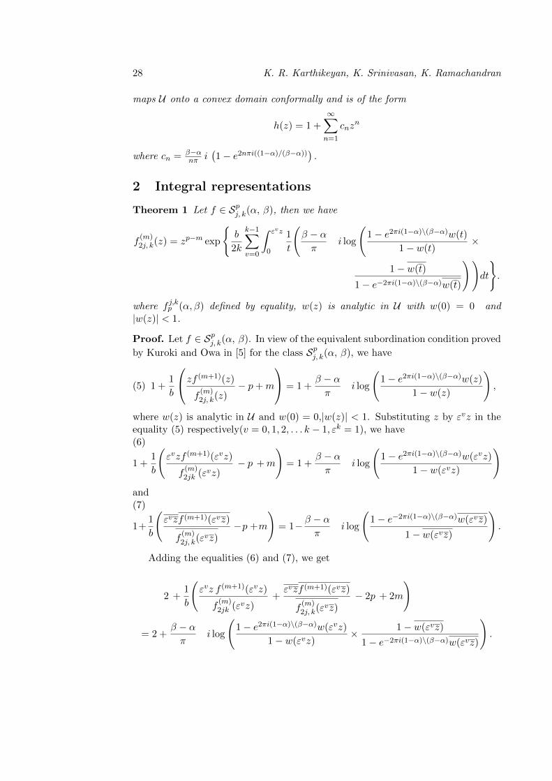
2 Integral representations
Theorem 1 Let f ∈ Spj, k(α, β), then we have
f(m)2j, k(z) = zp−m exp
{b
2k
k−1∑v=0
∫ εvz
0
1
t
(β − απ
i log
(1− e2πi(1−α)\(β−α)w(t)
1− w(t)×
1− w(t)
1− e−2πi(1−α)\(β−α)w(t)
))dt
}.
where f j,kp (α, β) defined by equality, w(z) is analytic in U with w(0) = 0 and|w(z)| < 1.
Proof. Let f ∈ Spj, k(α, β). In view of the equivalent subordination condition proved
by Kuroki and Owa in [5] for the class Spj, k(α, β), we have
(5) 1 +1
b
zf (m+1)(z)
f(m)2j, k(z)
− p+m
= 1 +β − απ
i log
(1− e2πi(1−α)\(β−α)w(z)
1− w(z)
),
where w(z) is analytic in U and w(0) = 0,|w(z)| < 1. Substituting z by εvz in theequality (5) respectively(v = 0, 1, 2, . . . k − 1, εk = 1), we have(6)
1 +1
b
(εvzf (m+1)(εvz)
f(m)2jk (εvz)
− p +m
)= 1 +
β − απ
i log
(1− e2πi(1−α)\(β−α)w(εvz)
1− w(εvz)
)and(7)
1+1
b
(εvzf (m+1)(εvz)
f(m)2j, k(ε
vz)−p +m
)= 1− β − α
πi log
(1− e−2πi(1−α)\(β−α)w(εvz)
1− w(εvz)
).
Adding the equalities (6) and (7), we get
2 +1
b
(εvz f (m+1)(εvz)
f(m)2jk (εvz)
+εvzf (m+1)(εvz)
f(m)2j, k(ε
vz)− 2p + 2m
)
= 2 +β − απ
i log
(1− e2πi(1−α)\(β−α)w(εvz)
1− w(εvz)× 1− w(εvz)
1− e−2πi(1−α)\(β−α)w(εvz)
).
Some Classes Of Multivalent Starlike Functions And Convex Functions 29
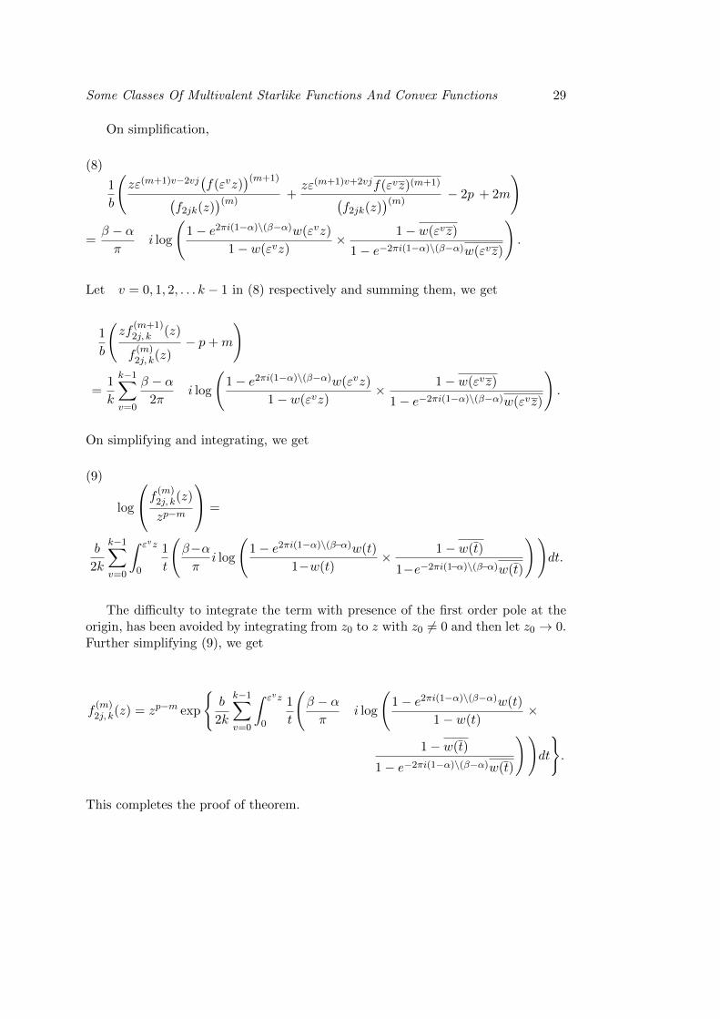
On simplification,
(8)
1
b
(zε(m+1)v−2vj(f(εvz)
)(m+1)(f2jk(z)
)(m)+zε(m+1)v+2vjf(εvz)(m+1)(
f2jk(z))(m)
− 2p + 2m
)
=β − απ
i log
(1− e2πi(1−α)\(β−α)w(εvz)
1− w(εvz)× 1− w(εvz)
1− e−2πi(1−α)\(β−α)w(εvz)
).
Let v = 0, 1, 2, . . . k − 1 in (8) respectively and summing them, we get
1
b
(zf
(m+1)2j, k (z)
f(m)2j, k(z)
− p+m
)
=1
k
k−1∑v=0
β − α2π
i log
(1− e2πi(1−α)\(β−α)w(εvz)
1− w(εvz)× 1− w(εvz)
1− e−2πi(1−α)\(β−α)w(εvz)
).
On simplifying and integrating, we get
(9)
log
f (m)2j, k(z)
zp−m
=
b
2k
k−1∑v=0
∫ εvz
0
1
t
(β−απ
i log
(1− e2πi(1−α)\(β−α)w(t)
1−w(t)× 1− w(t)
1−e−2πi(1−α)\(β−α)w(t)
))dt.
The difficulty to integrate the term with presence of the first order pole at theorigin, has been avoided by integrating from z0 to z with z0 6= 0 and then let z0 → 0.Further simplifying (9), we get
f(m)2j, k(z) = zp−m exp
{b
2k
k−1∑v=0
∫ εvz
0
1
t
(β − απ
i log
(1− e2πi(1−α)\(β−α)w(t)
1− w(t)×
1− w(t)
1− e−2πi(1−α)\(β−α)w(t)
))dt
}.
This completes the proof of theorem.
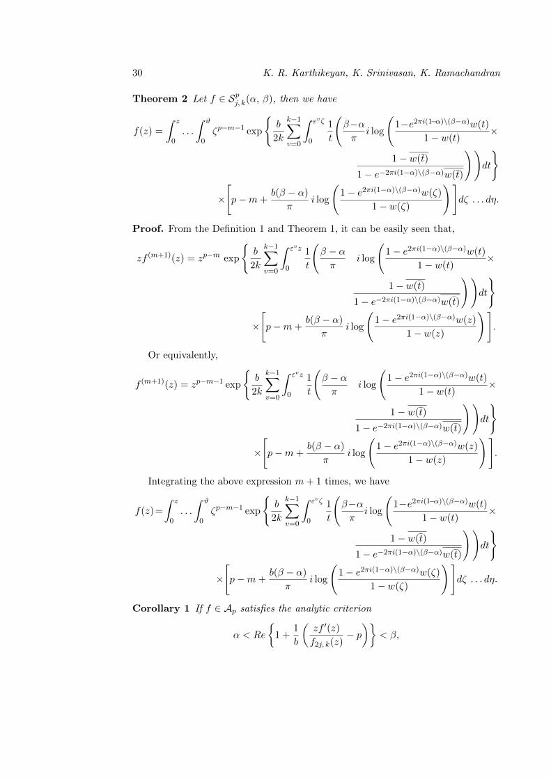
30 K. R. Karthikeyan, K. Srinivasan, K. Ramachandran
Theorem 2 Let f ∈ Spj, k(α, β), then we have
f(z) =
∫ z
0. . .
∫ ϑ
0ζp−m−1 exp
{b
2k
k−1∑v=0
∫ εvζ
0
1
t
(β−απ
i log
(1−e2πi(1−α)\(β−α)w(t)
1− w(t)×
1− w(t)
1− e−2πi(1−α)\(β−α)w(t)
))dt
}
×
[p−m+
b(β − α)
πi log
(1− e2πi(1−α)\(β−α)w(ζ)
1− w(ζ)
)]dζ . . . dη.
Proof. From the Definition 1 and Theorem 1, it can be easily seen that,
zf (m+1)(z) = zp−m exp
{b
2k
k−1∑v=0
∫ εvz
0
1
t
(β − απ
i log
(1− e2πi(1−α)\(β−α)w(t)
1− w(t)×
1− w(t)
1− e−2πi(1−α)\(β−α)w(t)
))dt
}
×
[p−m+
b(β − α)
πi log
(1− e2πi(1−α)\(β−α)w(z)
1− w(z)
)].
Or equivalently,
f (m+1)(z) = zp−m−1 exp
{b
2k
k−1∑v=0
∫ εvz
0
1
t
(β − απ
i log
(1− e2πi(1−α)\(β−α)w(t)
1− w(t)×
1− w(t)
1− e−2πi(1−α)\(β−α)w(t)
))dt
}
×
[p−m+
b(β − α)
πi log
(1− e2πi(1−α)\(β−α)w(z)
1− w(z)
)].
Integrating the above expression m+ 1 times, we have
f(z)=
∫ z
0. . .
∫ ϑ
0ζp−m−1 exp
{b
2k
k−1∑v=0
∫ εvζ
0
1
t
(β−απ
i log
(1−e2πi(1−α)\(β−α)w(t)
1− w(t)×
1− w(t)
1− e−2πi(1−α)\(β−α)w(t)
))dt
}
×
[p−m+
b(β − α)
πi log
(1− e2πi(1−α)\(β−α)w(ζ)
1− w(ζ)
)]dζ . . . dη.
Corollary 1 If f ∈ Ap satisfies the analytic criterion
α < Re
{1 +
1
b
(zf ′(z)
f2j, k(z)− p)}
< β,
Some Classes Of Multivalent Starlike Functions And Convex Functions 31
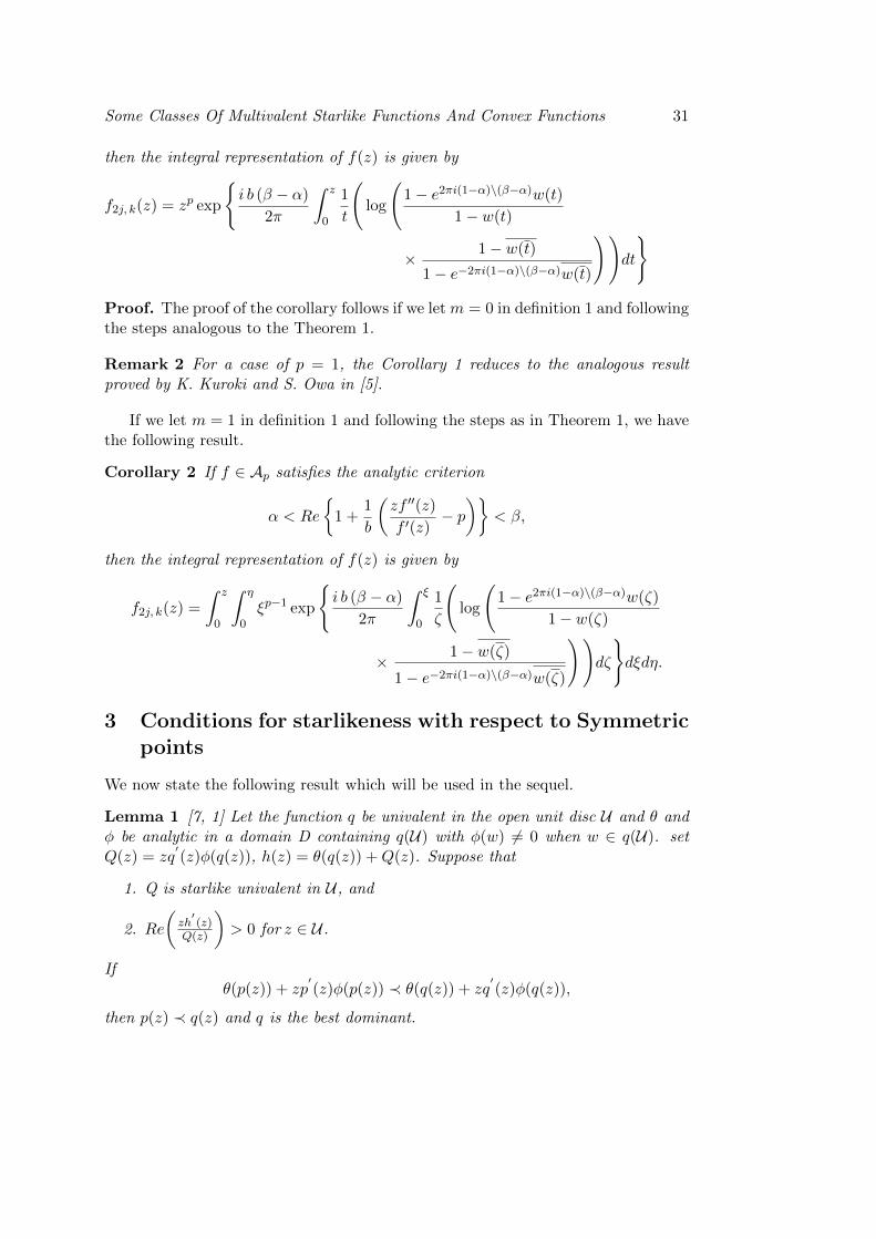
then the integral representation of f(z) is given by
f2j, k(z) = zp exp
{i b (β − α)
2π
∫ z
0
1
t
(log
(1− e2πi(1−α)\(β−α)w(t)
1− w(t)
× 1− w(t)
1− e−2πi(1−α)\(β−α)w(t)
))dt
}
Proof. The proof of the corollary follows if we let m = 0 in definition 1 and followingthe steps analogous to the Theorem 1.
Remark 2 For a case of p = 1, the Corollary 1 reduces to the analogous resultproved by K. Kuroki and S. Owa in [5].
If we let m = 1 in definition 1 and following the steps as in Theorem 1, we havethe following result.
Corollary 2 If f ∈ Ap satisfies the analytic criterion
α < Re
{1 +
1
b
(zf ′′(z)
f ′(z)− p)}
< β,
then the integral representation of f(z) is given by
f2j, k(z) =
∫ z
0
∫ η
0ξp−1 exp
{i b (β − α)
2π
∫ ξ
0
1
ζ
(log
(1− e2πi(1−α)\(β−α)w(ζ)
1− w(ζ)
× 1− w(ζ)
1− e−2πi(1−α)\(β−α)w(ζ)
))dζ
}dξdη.
3 Conditions for starlikeness with respect to Symmetricpoints
We now state the following result which will be used in the sequel.
Lemma 1 [7, 1] Let the function q be univalent in the open unit disc U and θ andφ be analytic in a domain D containing q(U) with φ(w) 6= 0 when w ∈ q(U). setQ(z) = zq
′(z)φ(q(z)), h(z) = θ(q(z)) +Q(z). Suppose that
1. Q is starlike univalent in U , and
2. Re
(zh
′(z)
Q(z)
)> 0 for z ∈ U .
Ifθ(p(z)) + zp
′(z)φ(p(z)) ≺ θ(q(z)) + zq
′(z)φ(q(z)),
then p(z) ≺ q(z) and q is the best dominant.
32 K. R. Karthikeyan, K. Srinivasan, K. Ramachandran
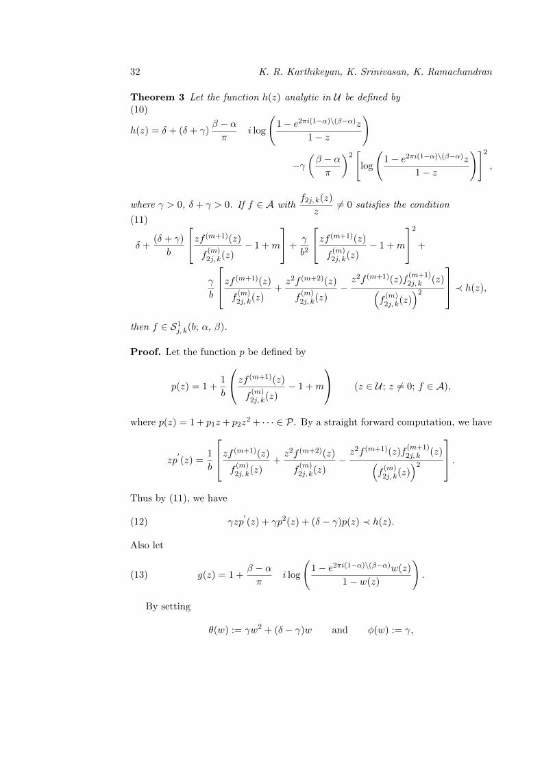
Theorem 3 Let the function h(z) analytic in U be defined by(10)
h(z) = δ + (δ + γ)β − απ
i log
(1− e2πi(1−α)\(β−α)z
1− z
)
−γ(β − απ
)2[
log
(1− e2πi(1−α)\(β−α)z
1− z
)]2,
where γ > 0, δ + γ > 0. If f ∈ A withf2j, k(z)
z6= 0 satisfies the condition
(11)
δ +(δ + γ)
b
zf (m+1)(z)
f(m)2j, k(z)
− 1 +m
+γ
b2
zf (m+1)(z)
f(m)2j, k(z)
− 1 +m
2
+
γ
b
zf (m+1)(z)
f(m)2j, k(z)
+z2f (m+2)(z)
f(m)2j, k(z)
−z2f (m+1)(z)f
(m+1)2j, k (z)(
f(m)2j, k(z)
)2 ≺ h(z),
then f ∈ S1j, k(b; α, β).
Proof. Let the function p be defined by
p(z) = 1 +1
b
zf (m+1)(z)
f(m)2j, k(z)
− 1 +m
(z ∈ U ; z 6= 0; f ∈ A),
where p(z) = 1 + p1z+ p2z2 + · · · ∈ P. By a straight forward computation, we have
zp′(z) =
1
b
zf (m+1)(z)
f(m)2j, k(z)
+z2f (m+2)(z)
f(m)2j, k(z)
−z2f (m+1)(z)f
(m+1)2j, k (z)(
f(m)2j, k(z)
)2 .
Thus by (11), we have
(12) γzp′(z) + γp2(z) + (δ − γ)p(z) ≺ h(z).
Also let
(13) g(z) = 1 +β − απ
i log
(1− e2πi(1−α)\(β−α)w(z)
1− w(z)
).
By setting
θ(w) := γw2 + (δ − γ)w and φ(w) := γ,
Some Classes Of Multivalent Starlike Functions And Convex Functions 33
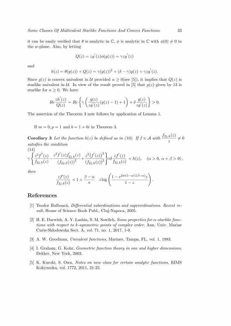
it can be easily verified that θ is analytic in C, φ is analytic in C with φ(0) 6= 0 inthe w-plane. Also, by letting
Q(z) = zg′(z)φ(g(z)) = γzg
′(z)
and
h(z) = θ(g(z)) +Q(z) = γ(g(z))2 + (δ − γ)g(z) + γzg′(z).
Since g(z) is convex univalent in U provided α ≥ 0(see [5]), it implies that Q(z) isstarlike univalent in U . In view of the result proved in [5] that g(z) given by 13 isstarlike for α ≥ 0. We have
Rezh
′(z)
Q(z)= Re
{γ
(g(z)
zg′(z)(g(z)− 1) + 1
)+ δ
g(z)
zg′(z)
}> 0.
The assertion of the Theorem 3 now follows by application of Lemma 1.
If m = 0, p = 1 and b = 1 + 0i in Theorem 3.
Corollary 3 Let the function h(z) be defined as in (10). If f ∈ A withf2j, k(z)
z6= 0
satisfies the condition(14)
γ
{z2f
′′(z)
f2j, k(z)−z2f
′(z)f
′2j, k(z)
(f2j, k(z))2 +
z2(f
′(z))2
(f2j, k(z))2
}+δ
zf′(z)
f2j, k(z)≺ h(z), (α > 0, α+ β > 0) ,
thenzf ′(z)
f2j, k(z)≺ 1 +
β − απ
i log
(1− e2πi(1−α)\(β−α)z
1− z
).
References
[1] Teodor Bulboaca, Differential subordinations and superordinations. Recent re-sult, House of Science Book Publ., Cluj-Napoca, 2005.
[2] H. E. Darwish, A. Y. Lashin, S. M. Sowileh, Some properties for α-starlike func-tions with respect to k-symmetric points of complex order, Ann. Univ. MariaeCurie-Sk lodowska Sect. A, vol. 71, no. 1, 2017, 1-9.
[3] A. W. Goodman, Univalent functions, Mariner, Tampa, FL, vol. 1, 1983.
[4] I. Graham, G. Kohr, Geometric function theory in one and higher dimensions,Dekker, New York, 2003.
[5] K. Kuroki, S. Owa, Notes on new class for certain analytic functions, RIMSKokyuroku, vol. 1772, 2011, 21-25.
34 K. R. Karthikeyan, K. Srinivasan, K. Ramachandran
[6] P. Liczberski, J. Po lubinski, On (j, k)-symmetrical functions, Math. Bohem.,vol. 120, no. 1, 1995, 13-28.
[7] S. S. Miller, P. T. Mocanu, Subordinants of differential superordinations, Com-plex Var. Theory Appl., vol. 48, no. 10, 2003, 815-826.
[8] M. A. Nasr, M. K. Aouf, Starlike function of complex order, J. Natur. Sci.Math., vol. 25, no. 1, 1985, 1-12.
[9] K. Sakaguchi, On a certain univalent mapping, J. Math. Soc. Japan, vol. 11,1959, 72-75.
[10] C. Selvaraj, K. R. Karthikeyan, G. Thirupathi, Multivalent functions with re-spect to symmetric conjugate points, Punjab Univ. J. Math. (Lahore), vol. 46,no. 1, 2014, 1-8.
[11] Z.-G. Wang, C.-Y. Gao, S.-M. Yuan, On certain subclasses of close-to-convexand quasi-convex functions with respect to k-symmetric points, J. Math. Anal.Appl., vol. 322, no. 1, 2006, 97-106.
[12] P. Wiatrowski, The coefficients of a certain family of holomorphic functions,Zeszyty Nauk. Uniw. Lodz. Nauki Mat. Przyrod. Ser. II, no. 39, 1971, 75-85.
K. R. KarthikeyanCaledonian College of EngineeringDepartment of Mathematics and StatisticsMuscat, Sultanate of Oman.e-mail: kr [email protected]
K. SrinivasanPresidency College (Autonomous)Department of MathematicsChennai-600005, Tamilnadu, India.
K. RamachandranSRM UniversityDepartment of MathematicsRamapuram, Chennai-600089, Tamilnadu, India.e-mail: [email protected]
General Mathematics Vol. 26, No. 1-2 (2018), 35–39
A remark on some combinatorial identities 1
Ulrich Abel, Georg Arends
Abstract
Recently, Barar presented new families of rational and polynomial Heunfunctions. As an application she derived two interesting combinatorial identi-ties. We give an independent proof of a generalization which gives insight intothe structure of the expressions.
2010 Mathematics Subject Classification: 05A19.Key words and phrases: Combinatorial identities.
1 Introduction
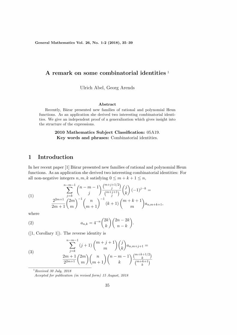
In her recent paper [1] Barar presented new families of rational and polynomial Heunfunctions. As an application she derived two interesting combinatorial identities: Forall non-negative integers n,m, k satisfying 0 ≤ m + k + 1 ≤ n,
(1)
n−m−1∑j=k
(n−m− 1
j
)(m+j+1/2j
)(m+j+1
j
) (jk
)(−1)j−k =
22m+1
2m + 1
(2m
m
)−1( n
m + 1
)−1
(k + 1)
(m + k + 1
m
)an,m+k+1,
where
(2) an,k = 4−n
(2k
k
)(2n− 2k
n− k
).
([1, Corollary 1]). The reverse identity is
(3)
n−m−1∑j=k
(j + 1)
(m + j + 1
m
)(j
k
)an,m+j+1 =
2m + 1
22m+1
(2m
m
)(n
m + 1
)(n−m− 1
k
)(m+k+1/2k
)(m+k+1
k
)1Received 30 July, 2018Accepted for publication (in revised form) 15 August, 2018
35
36 Ulrich Abel, Georg Arends
([1, Corollary 2]).Further investigations on Heun functions, in particular closed forms, explicit
expressions, or representations in terms of hypergeometric functions can be found inthe paper [2] by Barar, Mocanu and Rasa. The same authors presented in the paper[3] a plenty of combinatorial identities which were derived by comparing differentexpressions of the same Heun function.
The purpose of this note is a direct proof of identity (1) in a more general formyielding a concise expression of the right-hand side. Moreover, we observe thatidentity (3) is a consequence of the binomial inversion.
We derive the following result.
2 Main result
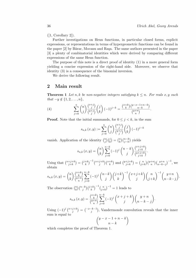
Theorem 1 Let n, k be non-negative integers satisfying k ≤ n. For reals x, y suchthat −y /∈ {1, 2, . . . , n},
(4)
n∑j=0
(n
j
)(x+jj
)(y+jj
)(jk
)(−1)j−k =
(x+kk
)(y−x−1+n−k
n−k
)(y+nn
) .
Proof. Note that the initial summands, for 0 ≤ j < k, in the sum
sn,k (x, y) :=n∑
j=0
(n
j
)(x+jj
)(y+jj
)(jk
)(−1)j−k
vanish. Application of the identity(nj
)(jk
)=(nk
)(n−kj−k
)yields
sn,k (x, y) =
(n
k
) n−k∑j=0
(−1)j(n− k
j
)(x+j+kj+k
)(y+j+kj+k
) .Using that
(x+j+kj+k
)=(j+kk
)−1(x+j+kj
)(x+kk
)and
(y+j+kj+k
)=(
nj+k
)(y+nn
)(y+n
n−k−j
)−1, we
obtain
sn,k (x, y) =
(n
k
)(x+kk
)(y+nn
) n−k∑j=0
(−1)j(n−kj
)(j+k
k
)−1(x+j+k
j
)(n
j+k
)−1( y+n
n−k−j
).
The observation(nk
)(n−kj
)(j+kk
)−1( nj+k
)−1= 1 leads to
sn,k (x, y) =
(x+kk
)(y+nn
) n−k∑j=0
(−1)j(x + j + k
j
)(y + n
n− k − j
).
Using (−1)j(x+j+k
j
)=(−x−k−1
j
), Vandermonde convolution reveals that the inner
sum is equal to (y − x− 1 + n− k
n− k
)which completes the proof of Theorem 1.
A remark on some combinatorial identities 37
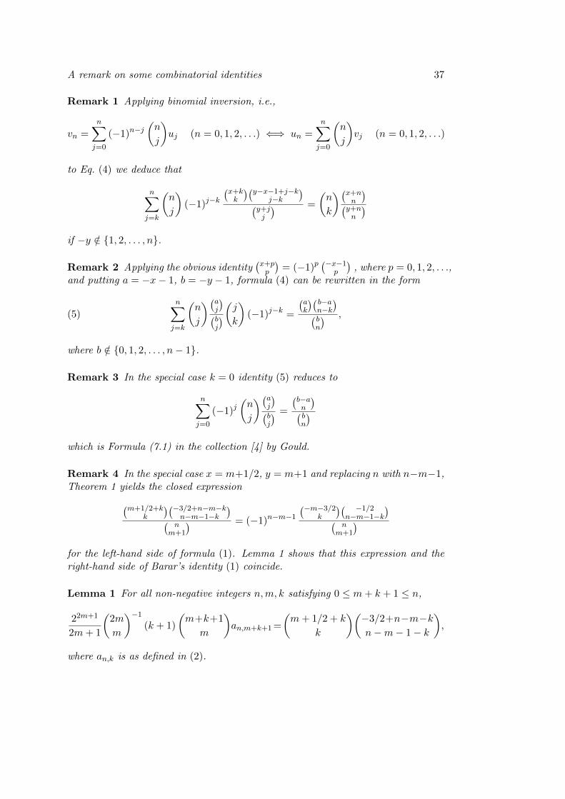
Remark 1 Applying binomial inversion, i.e.,
vn =n∑
j=0
(−1)n−j
(n
j
)uj (n = 0, 1, 2, . . .) ⇐⇒ un =
n∑j=0
(n
j
)vj (n = 0, 1, 2, . . .)
to Eq. (4) we deduce that
n∑j=k
(n
j
)(−1)j−k
(x+kk
)(y−x−1+j−k
j−k
)(y+jj
) =
(n
k
)(x+nn
)(y+nn
)if −y /∈ {1, 2, . . . , n}.
Remark 2 Applying the obvious identity(x+pp
)= (−1)p
(−x−1p
), where p = 0, 1, 2, . . .,
and putting a = −x− 1, b = −y − 1, formula (4) can be rewritten in the form
(5)
n∑j=k
(n
j
)(aj
)(bj
)(jk
)(−1)j−k =
(ak
)(b−an−k
)(bn
) ,
where b /∈ {0, 1, 2, . . . , n− 1}.
Remark 3 In the special case k = 0 identity (5) reduces to
n∑j=0
(−1)j(n
j
)(aj
)(bj
) =
(b−an
)(bn
)which is Formula (7.1) in the collection [4] by Gould.
Remark 4 In the special case x = m+1/2, y = m+1 and replacing n with n−m−1,Theorem 1 yields the closed expression(m+1/2+k
k
)(−3/2+n−m−kn−m−1−k
)(n
m+1
) = (−1)n−m−1
(−m−3/2k
)( −1/2n−m−1−k
)(n
m+1
)for the left-hand side of formula (1). Lemma 1 shows that this expression and theright-hand side of Barar’s identity (1) coincide.
Lemma 1 For all non-negative integers n,m, k satisfying 0 ≤ m + k + 1 ≤ n,
22m+1
2m + 1
(2m
m
)−1
(k + 1)
(m+k+1
m
)an,m+k+1=
(m + 1/2 + k
k
)(−3/2+n−m−kn−m− 1− k
),
where an,k is as defined in (2).
38 Ulrich Abel, Georg Arends
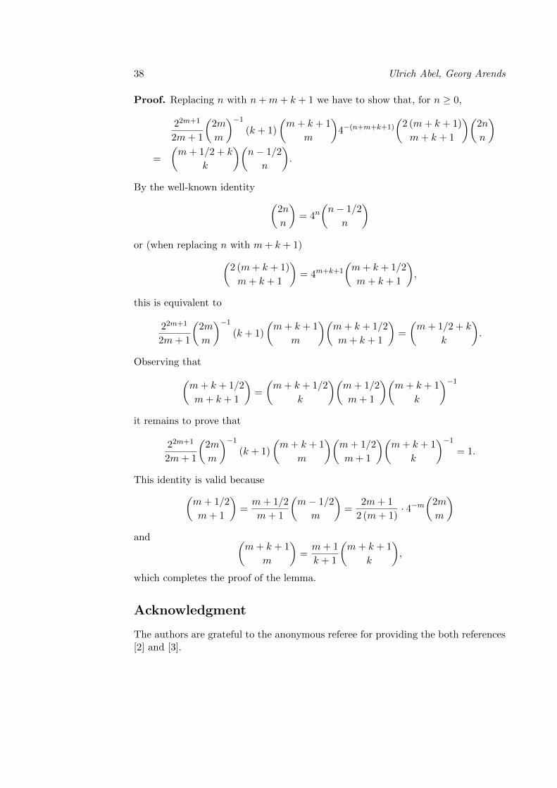
Proof. Replacing n with n + m + k + 1 we have to show that, for n ≥ 0,
22m+1
2m + 1
(2m
m
)−1
(k + 1)
(m + k + 1
m
)4−(n+m+k+1)
(2 (m + k + 1)
m + k + 1
)(2n
n
)=
(m + 1/2 + k
k
)(n− 1/2
n
).
By the well-known identity (2n
n
)= 4n
(n− 1/2
n
)or (when replacing n with m + k + 1)(
2 (m + k + 1)
m + k + 1
)= 4m+k+1
(m + k + 1/2
m + k + 1
),
this is equivalent to
22m+1
2m + 1
(2m
m
)−1
(k + 1)
(m + k + 1
m
)(m + k + 1/2
m + k + 1
)=
(m + 1/2 + k
k
).
Observing that(m + k + 1/2
m + k + 1
)=
(m + k + 1/2
k
)(m + 1/2
m + 1
)(m + k + 1
k
)−1
it remains to prove that
22m+1
2m + 1
(2m
m
)−1
(k + 1)
(m + k + 1
m
)(m + 1/2
m + 1
)(m + k + 1
k
)−1
= 1.
This identity is valid because(m + 1/2
m + 1
)=
m + 1/2
m + 1
(m− 1/2
m
)=
2m + 1
2 (m + 1)· 4−m
(2m
m
)and (
m + k + 1
m
)=
m + 1
k + 1
(m + k + 1
k
),
which completes the proof of the lemma.
Acknowledgment
The authors are grateful to the anonymous referee for providing the both references[2] and [3].
A remark on some combinatorial identities 39
References
[1] A. Barar, Some families of rational Heun functions and combinatorial identities,General Mathematics, vol. 25, no. 1-2, 2017, 29-36.
[2] A. Barar, G. R. Mocanu, I. Rasa, Heun functions related to entropies, Rev.R. Acad. Cienc. Exactas Fıs. Nat. Ser. A Math. RACSAM, 2018, 1-12.https://doi.org/10.1007/s13398-018-0516-x.
[3] A. Barar, G. R. Mocanu, I. Rasa, Heun functions and combinatorial identities,2018, arXiv:1801.05054.
[4] H. W. Gould, Combinatorial Identities, Morgantown Print & Bind., Morgan-town, WV, 1972.
Ulrich AbelTechnische Hochschule MittelhessenFachbereich Mathematik, Naturwissenschaften und DatenverarbeitungWilhelm-Leuschner-Straße 13, 61169 Friedberg, Germanye-mail: [email protected]
Georg Arends52249 Eschweiler, Germanye-mail: [email protected]

General Mathematics Vol. 26, No. 1-2 (2018), 41–55
Refinements of Bullen-Type Inequalities for DifferentKind of Convex Functions via Riemann-Liouville
Fractional Integrals Involving Gauss HypergeometricFunction 1
Musa Cakmak
Abstract
In this paper, the author establishes a new identity for differentiable func-tions and obtain some new inequalities for differentiable functions based ons-convexity, m-convexity and (,m)-convexity via Riemann-Liouville fractionalintegrals involving Gauss hypergeometric function.
2010 Mathematics Subject Classification: 26D07, 26D10, 26D15.Key words and phrases: Bullen’s inequality, s-convex function, m-convexfunction, (,m)-convex function, Power-mean inequality, Riemann-Liouville
fractional integrals.
1 Introduction
Let f : I ⊆ R→ R be a convex mapping defined on the interval I of real numbersand a, b ∈ I, with a < b. The following double inequalities:
(HH) f
(a+ b
2
)≤ 1
b− a
∫ b
af (x) dx ≤ f (a) + f (b)
2
hold. In the literature, this double inequalities are known as the Hermite-Hadamardinequality for convex functions.Many important inequalities are established for theclass of convex functions, but one of the most famous is so called Hermite-Hadamard’sinequality (or Hadamard’s inequality). For the development and use of this inequal-ity, in recent years many authors established several inequalities connected to thisfact. For recent results, refinements, counterparts, generalizations and new Hermite-Hadamard type inequalities see [1]-[12], [16] and [21]-[25].
1Received 18 June, 2018Accepted for publication (in revised form) 10 August, 2018
41
42 Musa Cakmak
The following inequality is well known in the literature as Bullen’s inequality(see for example [9, p.10]);
(B)1
b− a
∫ b
af (κ) dκ ≤ 1
2
[f (a) + f (b)
2+ f
(a+ b
2
)],
provided that f : [a, b]→ R is a convex function on [a, b].In this section we will present definitions, theorems, lemma and remarks used in
this paper.
Definition 1 [15, 17]Let I be an interval in R. Then f : I → R, ∅ 6= I ⊆ R is saidto be convex if
f (tx+ (1− t) y) ≤ tf (x) + (1− t) f (y) .
for all x, y ∈ I and t ∈ [0, 1].
Definition 2 [12] Let s ∈ (0, 1]. A function f : I ⊂ R0 = [0,∞)→ R0 is said to bes-convex in the second sense if
f (tx+ (1− t) y) ≤ tsf (x) + (1− t)s f (y)
for all x, y ∈ I and t ∈ [0, 1].It can be easily checked for s = 1, s-convexity reducesto the ordinary convexity of functions defined on [0,∞).
Definition 3 [22, 23] A function f : [0, b] → R is said to be m−convex, wherem ∈ [0, 1], if we have
f (tx+m (1− t) y) ≤ tf (x) +m (1− t) f (y)
for all x, y ∈ [0, b] and t ∈ [0, 1]. We say that f is m−concave if −f is m−convex.Denote by Km(b) the class of all m−convex functions on [0, b] for which f(0) ≤ 0.
Definition 4 [22, 23] The function f : [0, b] → R is said to be (α,m)−convex,where (α,m) ∈ [0, 1]2 , if for every x, y ∈ [0, b] and t ∈ [0, 1] , we have
f (tx+m (1− t) y) ≤ tαf (x) +m (1− tα) f (y) .
Denote by Kαm(b) the set of the (α,m)−convex functions on [0, b] for which f(0) ≤
0. We say that f is (α,m)−concave if −f is (α,m)−convex. Denote by Kαm(b) the
class of all (α,m)−convex functions on [0, b] for which f(0) ≤ 0.
Lemma 1 [3]Let f : I → R, I ⊂ R be a differentiable mapping on I◦, and a, b ∈I, a < b. If f ′ ∈ L1 ([a.b]) , t ∈ [0, 1] then∫ 1
0(1− 2t)
[(f ′(ta+ (1− t)
(a+ b
2
))+ f ′
(t
(a+ b
2
)+ (1− t) b
))]dt
=4
(b− a)
(f (a) + f (b)
2+ f
(a+ b
2
)− 2
b− a
∫ b
af (x) dx
).
Here I◦ denotes the interior of I.
Bullen-Type Inequalities via Riemann-Liouville Fractional Integrals 43
Theorem 1 [19]Let f : [a, b] → R be a positive function with 0 ≤ a < b andf ∈ L1 [a, b] . If f is a convex function on [a, b], then the following inequalities forfractional integrals hold:
f
(a+ b
2
)≤ Γ (γ + 1)
2 (b− a)γ[Jγa+f (b) + Jγb−f (a)
]≤ f (a) + f (b)
2
with γ > 0.
Definition 5 [13]The hypergeometric function defined by
pFq (a1, a2, ..., ap; b1, b2, ..., bq;x) =
∞∑k=0
(a1)k ... (ap)k(b1)k ... (bq)k
xk
k!
includes, as special cases, many of the elementary special functions. The first resultis a representation of 2F1 in terms of the beta integral
β (a, b) =
∫ 1
0ta−1 (1− t)b−1 dt.
The hypergeometric function 2F1 is given by
2F1 (a, b; c;x) =1
β (b, c− b)
∫ 1
0tb−1 (1− t)c−b−1 (1− tx)−a dt.
Euler’s gamma function defined by
Γ (a) =
∫ ∞0
ta−1e−tdt.
and
β (a, b) =Γ (a) Γ (b)
Γ (a+ b), Re a > 0, Re b > 0.
Definition 6 [11, 14, 18]Let f ∈ L1 [a, b]. The Riemann-Liouville integrals Jγa+f
and Jγb−f of order γ > 0 with a ≥ 0 are defined by
Jγa+f (x) =1
Γ (γ)
∫ x
a(x− t)γ−1 f (t) dt, a < x
and
Jγb−f (x) =1
Γ (γ)
∫ b
x(t− x)γ−1 f (t) dt, x < b
respectively. Here Γ (γ) is the Gamma function and J0a+f (x) = J0
b−f (x) = f (x) .
44 Musa Cakmak
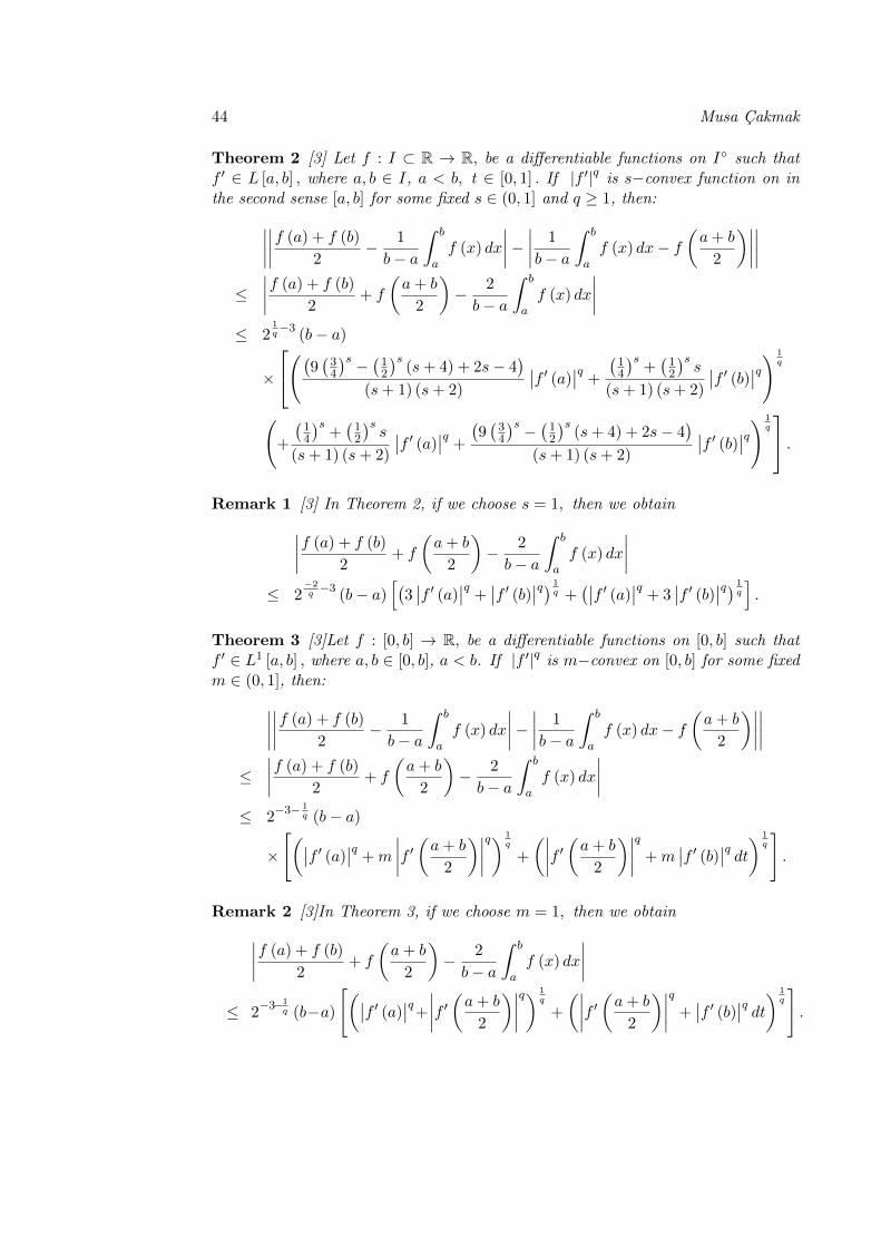
Theorem 2 [3] Let f : I ⊂ R → R, be a differentiable functions on I◦ such thatf ′ ∈ L [a, b] , where a, b ∈ I, a < b, t ∈ [0, 1] . If |f ′|q is s−convex function on inthe second sense [a, b] for some fixed s ∈ (0, 1] and q ≥ 1, then:∣∣∣∣∣∣∣∣f (a) + f (b)
2− 1
b− a
∫ b
af (x) dx
∣∣∣∣− ∣∣∣∣ 1
b− a
∫ b
af (x) dx− f
(a+ b
2
)∣∣∣∣∣∣∣∣≤
∣∣∣∣f (a) + f (b)
2+ f
(a+ b
2
)− 2
b− a
∫ b
af (x) dx
∣∣∣∣≤ 2
1q−3
(b− a)
×
((9 (34)s − (12)s (s+ 4) + 2s− 4)
(s+ 1) (s+ 2)
∣∣f ′ (a)∣∣q +
(14
)s+(12
)ss
(s+ 1) (s+ 2)
∣∣f ′ (b)∣∣q) 1q
(+
(14
)s+(12
)ss
(s+ 1) (s+ 2)
∣∣f ′ (a)∣∣q +
(9(34
)s − (12)s (s+ 4) + 2s− 4)
(s+ 1) (s+ 2)
∣∣f ′ (b)∣∣q) 1q
.Remark 1 [3] In Theorem 2, if we choose s = 1, then we obtain∣∣∣∣f (a) + f (b)
2+ f
(a+ b
2
)− 2
b− a
∫ b
af (x) dx
∣∣∣∣≤ 2
−2q−3
(b− a)[(
3∣∣f ′ (a)
∣∣q +∣∣f ′ (b)∣∣q) 1
q +(∣∣f ′ (a)
∣∣q + 3∣∣f ′ (b)∣∣q) 1
q
].
Theorem 3 [3]Let f : [0, b] → R, be a differentiable functions on [0, b] such thatf ′ ∈ L1 [a, b] , where a, b ∈ [0, b], a < b. If |f ′|q is m−convex on [0, b] for some fixedm ∈ (0, 1], then:∣∣∣∣∣∣∣∣f (a) + f (b)
2− 1
b− a
∫ b
af (x) dx
∣∣∣∣− ∣∣∣∣ 1
b− a
∫ b
af (x) dx− f
(a+ b
2
)∣∣∣∣∣∣∣∣≤
∣∣∣∣f (a) + f (b)
2+ f
(a+ b
2
)− 2
b− a
∫ b
af (x) dx
∣∣∣∣≤ 2
−3− 1q (b− a)
×
[(∣∣f ′ (a)∣∣q +m
∣∣∣∣f ′(a+ b
2
)∣∣∣∣q) 1q
+
(∣∣∣∣f ′(a+ b
2
)∣∣∣∣q +m∣∣f ′ (b)∣∣q dt) 1
q
].
Remark 2 [3]In Theorem 3, if we choose m = 1, then we obtain∣∣∣∣f (a) + f (b)
2+ f
(a+ b
2
)− 2
b− a
∫ b
af (x) dx
∣∣∣∣≤ 2
−3−1q (b−a)
[(∣∣f ′ (a)∣∣q+∣∣∣∣f ′(a+ b
2
)∣∣∣∣q) 1q
+
(∣∣∣∣f ′(a+ b
2
)∣∣∣∣q +∣∣f ′ (b)∣∣q dt) 1
q
].
Bullen-Type Inequalities via Riemann-Liouville Fractional Integrals 45
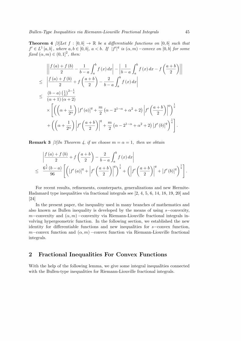
Theorem 4 [3]Let f : [0, b] → R be a differentiable functions on [0, b] such thatf ′ ∈ L1 [a, b] , where a, b ∈ [0, b], a < b. If |f ′|q is (α,m)−convex on [0, b] for somefixed (α,m) ∈ (0, 1]2, then:
∣∣∣∣∣∣∣∣f (a) + f (b)
2− 1
b− a
∫ b
af (x) dx
∣∣∣∣− ∣∣∣∣ 1
b− a
∫ b
af (x) dx− f
(a+ b
2
)∣∣∣∣∣∣∣∣≤
∣∣∣∣f (a) + f (b)
2+ f
(a+ b
2
)− 2
b− a
∫ b
af (x) dx
∣∣∣∣≤
(b− a)(14
)2− 1q
(α+ 1) (α+ 2)
×
[((α+
1
2α
) ∣∣f ′ (a)∣∣q +
m
2
(α− 21−α + α2 + 2
) ∣∣∣∣f ′(a+ b
2
)∣∣∣∣q) 1q
+
((α+
1
2α
) ∣∣∣∣f ′(a+ b
2
)∣∣∣∣q +m
2
(α− 21−α + α2 + 2
) ∣∣f ′ (b)∣∣q) 1q
].
Remark 3 [3]In Theorem 4, if we choose m = α = 1, then we obtain
∣∣∣∣f (a) + f (b)
2+ f
(a+ b
2
)− 2
b− a
∫ b
af (x) dx
∣∣∣∣≤ 6
1q (b− a)
96
[(∣∣f ′ (a)∣∣q +
∣∣∣∣f ′(a+ b
2
)∣∣∣∣q) 1q
+
(∣∣∣∣f ′(a+ b
2
)∣∣∣∣q +∣∣f ′ (b)∣∣q) 1
q
].
For recent results, refinements, counterparts, generalizations and new Hermite-Hadamard type inequalities via fractional integrals see [2, 4, 5, 6, 14, 18, 19, 20] and[24]
In the present paper, the inequality used in many branches of mathematics andalso known as Bullen inequality is developed by the means of using s−convexity,m−convexity and (α,m)−convexity via Riemann-Liouville fractional integrals in-volving hypergeometric function. In the following section, we established the newidentity for differentiable functions and new inequalities for s−convex function,m−convex function and (α,m)−convex function via Riemann-Liouville fractionalintegrals.
2 Fractional Inequalities For Convex Functions
With the help of the following lemma, we give some integral inequalities connectedwith the Bullen-type inequalities for Riemann-Liouville fractional integrals.
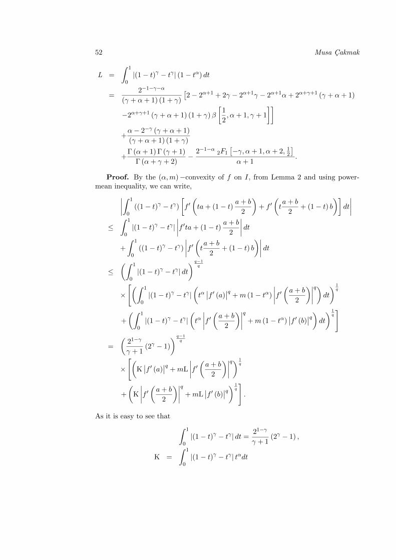
46 Musa Cakmak
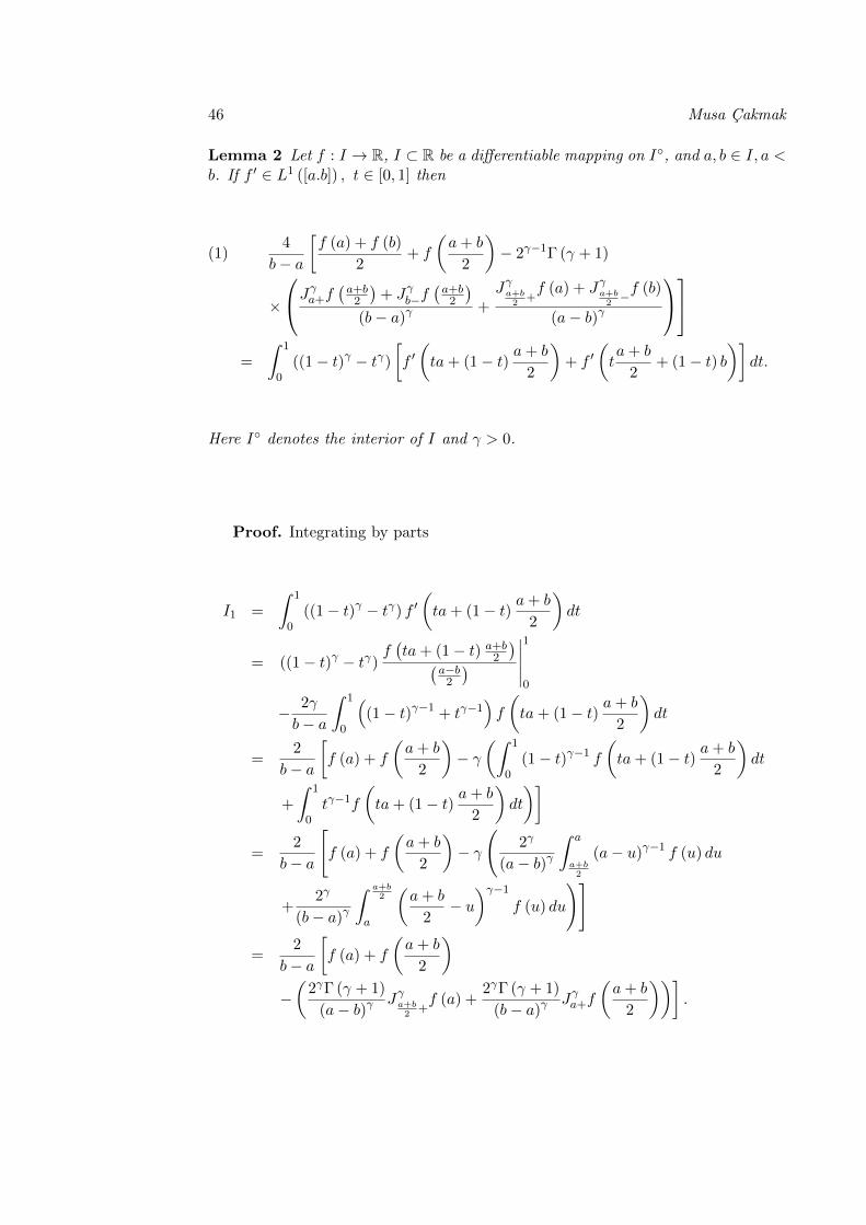
Lemma 2 Let f : I → R, I ⊂ R be a differentiable mapping on I◦, and a, b ∈ I, a <b. If f ′ ∈ L1 ([a.b]) , t ∈ [0, 1] then
4
b− a
[f (a) + f (b)
2+ f
(a+ b
2
)− 2γ−1Γ (γ + 1)(1)
×
Jγa+f (a+b2 )+ Jγb−f(a+b2
)(b− a)γ
+Jγa+b
2+f (a) + Jγa+b
2−f (b)
(a− b)γ
=
∫ 1
0((1− t)γ − tγ)
[f ′(ta+ (1− t) a+ b
2
)+ f ′
(ta+ b
2+ (1− t) b
)]dt.
Here I◦ denotes the interior of I and γ > 0.
Proof. Integrating by parts
I1 =
∫ 1
0((1− t)γ − tγ) f ′
(ta+ (1− t) a+ b
2
)dt
= ((1− t)γ − tγ)f(ta+ (1− t) a+b2
)(a−b2
) ∣∣∣∣∣1
0
− 2γ
b− a
∫ 1
0
((1− t)γ−1 + tγ−1
)f
(ta+ (1− t) a+ b
2
)dt
=2
b− a
[f (a) + f
(a+ b
2
)− γ
(∫ 1
0(1− t)γ−1 f
(ta+ (1− t) a+ b
2
)dt
+
∫ 1
0tγ−1f
(ta+ (1− t) a+ b
2
)dt
)]=
2
b− a
[f (a) + f
(a+ b
2
)− γ
(2γ
(a− b)γ∫ a
a+b2
(a− u)γ−1 f (u) du
+2γ
(b− a)γ
∫ a+b2
a
(a+ b
2− u)γ−1
f (u) du
)]
=2
b− a
[f (a) + f
(a+ b
2
)−(
2γΓ (γ + 1)
(a− b)γJγa+b
2+f (a) +
2γΓ (γ + 1)
(b− a)γJγa+f
(a+ b
2
))].
Bullen-Type Inequalities via Riemann-Liouville Fractional Integrals 47
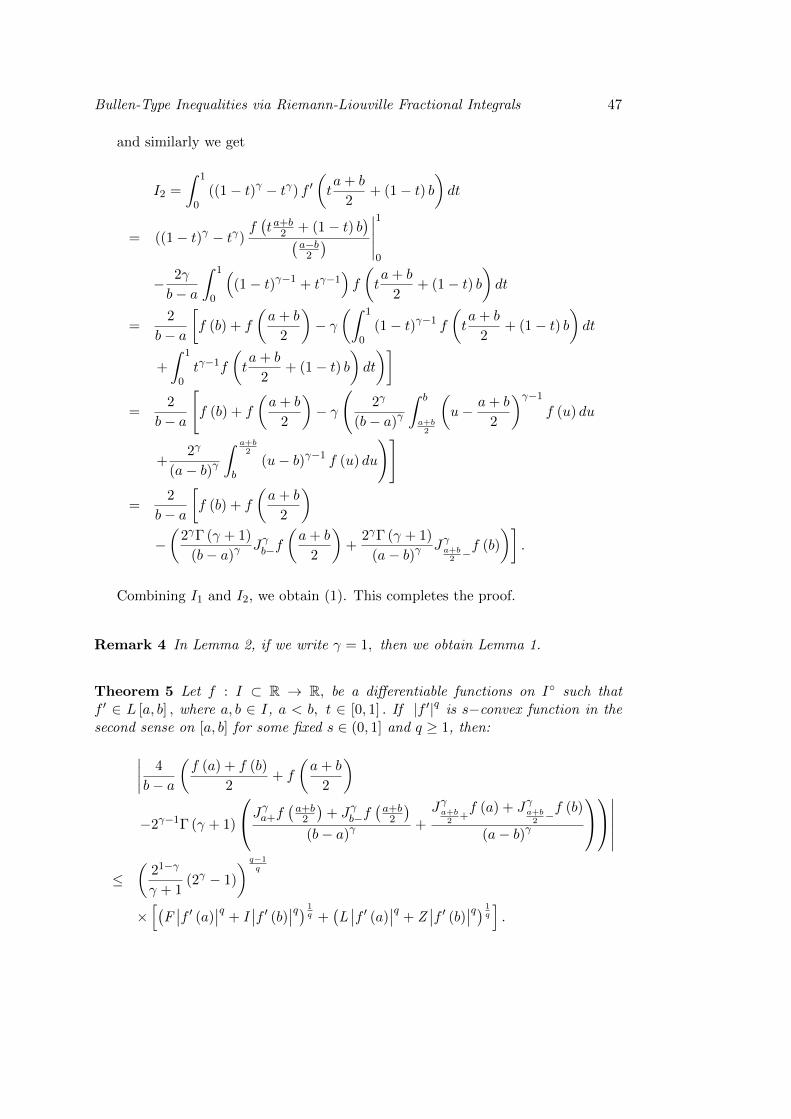
and similarly we get
I2 =
∫ 1
0((1− t)γ − tγ) f ′
(ta+ b
2+ (1− t) b
)dt
= ((1− t)γ − tγ)f(ta+b2 + (1− t) b
)(a−b2
) ∣∣∣∣∣1
0
− 2γ
b− a
∫ 1
0
((1− t)γ−1 + tγ−1
)f
(ta+ b
2+ (1− t) b
)dt
=2
b− a
[f (b) + f
(a+ b
2
)− γ
(∫ 1
0(1− t)γ−1 f
(ta+ b
2+ (1− t) b
)dt
+
∫ 1
0tγ−1f
(ta+ b
2+ (1− t) b
)dt
)]=
2
b− a
[f (b) + f
(a+ b
2
)− γ
(2γ
(b− a)γ
∫ b
a+b2
(u− a+ b
2
)γ−1f (u) du
+2γ
(a− b)γ∫ a+b
2
b(u− b)γ−1 f (u) du
)]
=2
b− a
[f (b) + f
(a+ b
2
)−(
2γΓ (γ + 1)
(b− a)γJγb−f
(a+ b
2
)+
2γΓ (γ + 1)
(a− b)γJγa+b
2−f (b)
)].
Combining I1 and I2, we obtain (1). This completes the proof.
Remark 4 In Lemma 2, if we write γ = 1, then we obtain Lemma 1.
Theorem 5 Let f : I ⊂ R → R, be a differentiable functions on I◦ such thatf ′ ∈ L [a, b] , where a, b ∈ I, a < b, t ∈ [0, 1] . If |f ′|q is s−convex function in thesecond sense on [a, b] for some fixed s ∈ (0, 1] and q ≥ 1, then:
∣∣∣∣ 4
b− a
(f (a) + f (b)
2+ f
(a+ b
2
)
−2γ−1Γ (γ + 1)
Jγa+f (a+b2 )+ Jγb−f(a+b2
)(b− a)γ
+Jγa+b
2+f (a) + Jγa+b
2−f (b)
(a− b)γ
∣∣∣∣∣∣≤
(21−γ
γ + 1(2γ − 1)
) q−1q
×[(
F∣∣f ′ (a)
∣∣q + I∣∣f ′ (b)∣∣q) 1
q +(L∣∣f ′ (a)
∣∣q + Z∣∣f ′ (b)∣∣q) 1
q
].
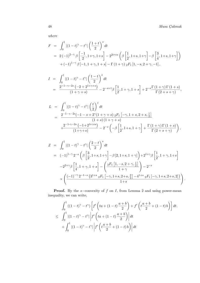
48 Musa Cakmak
where
F =
∫ 1
0|(1− t)γ − tγ |
(1 + t
2
)sdt
= 2 (−1)2−γ β
[−1
2, 1+γ, 1+s
]− 22+γ+s
(β
[1
2, 1+s, 1+γ
]−β
[3
4, 1+s, 1+γ
])+ (−1)1−γ β [−1, 1 + γ, 1 + s]− Γ (1 + γ) 2F1 [1,−s, 2 + γ,−1] ,
I =
∫ 1
0|(1− t)γ − tγ |
(1− t
2
)sdt
=2−1−γ−2s
(−2 + 21+γ+s
)(1 + γ + s)
− 2−s+1β
[1
2, 1 + γ, 1 + s
]+ 2−s
Γ (1 + γ) Γ (1 + s)
Γ (2 + s+ γ),
L =
∫ 1
0|(1− t)γ − tγ |
(t
2
)sdt
=2−1−γ−2s(−1− s+ 2γ(1 + γ + s) 2F1
[−γ, 1 + s, 2 + s, 12
](1 + s) (1 + γ + s)
+2−1−γ−2s
(−1+21+γ+s
)(1+γ+s)
− 2−s(−β[
1
2, 1+s, 1 + γ
]+
Γ (1 + γ) Γ (1 + s)
Γ (2 + s+ γ)
),
Z =
∫ 1
0|(1− t)γ − tγ |
(2− t
2
)sdt
= (−1)1−γ 2−s(β
[3
2, 1+s, 1+γ
]−β [2, 1+s, 1 + γ]
)+21+γβ
[1
2, 1 + γ, 1+s
]−22+γβ
[1
4, 1 + γ, 1 + s
]−
(2F1
[1,−s, 2 + γ, 12
]1 + γ
)− 2−s
×
((−1)−γ 2−1−s
(31+s 2F1
[−γ, 1+s, 2+s, 32
]−41+s 2F1 [−γ, 1+s, 2+s, 2]
)1+s
).
Proof. By the s−convexity of f on I, from Lemma 2 and using power-meaninequality, we can write,∫ 1
0((1− t)γ − tγ)
[f ′(ta+ (1− t) a+ b
2
)+ f ′
(ta+ b
2+ (1− t) b
)]dt.
≤∫ 1
0|(1− t)γ − tγ |
∣∣∣∣f ′(ta+ (1− t) a+ b
2
)∣∣∣∣ dt+
∫ 1
0|(1− t)γ − tγ |
∣∣∣∣f ′(ta+ b
2+ (1− t) b
)∣∣∣∣ dt
Bullen-Type Inequalities via Riemann-Liouville Fractional Integrals 49
≤(∫ 1
0|(1− t)γ − tγ | dt
) q−1q
×
[(∫ 1
0|(1− t)γ − tγ |
((1 + t
2
)s ∣∣f ′ (a)∣∣q +
(1− t
2
)s ∣∣f ′ (b)∣∣q)) 1q
dt
+
(∫ 1
0|(1− t)γ − tγ |
((t
2
)s ∣∣f ′ (a)∣∣q +
(2− t
2
)s ∣∣f ′ (b)∣∣q)) 1q
dt
]
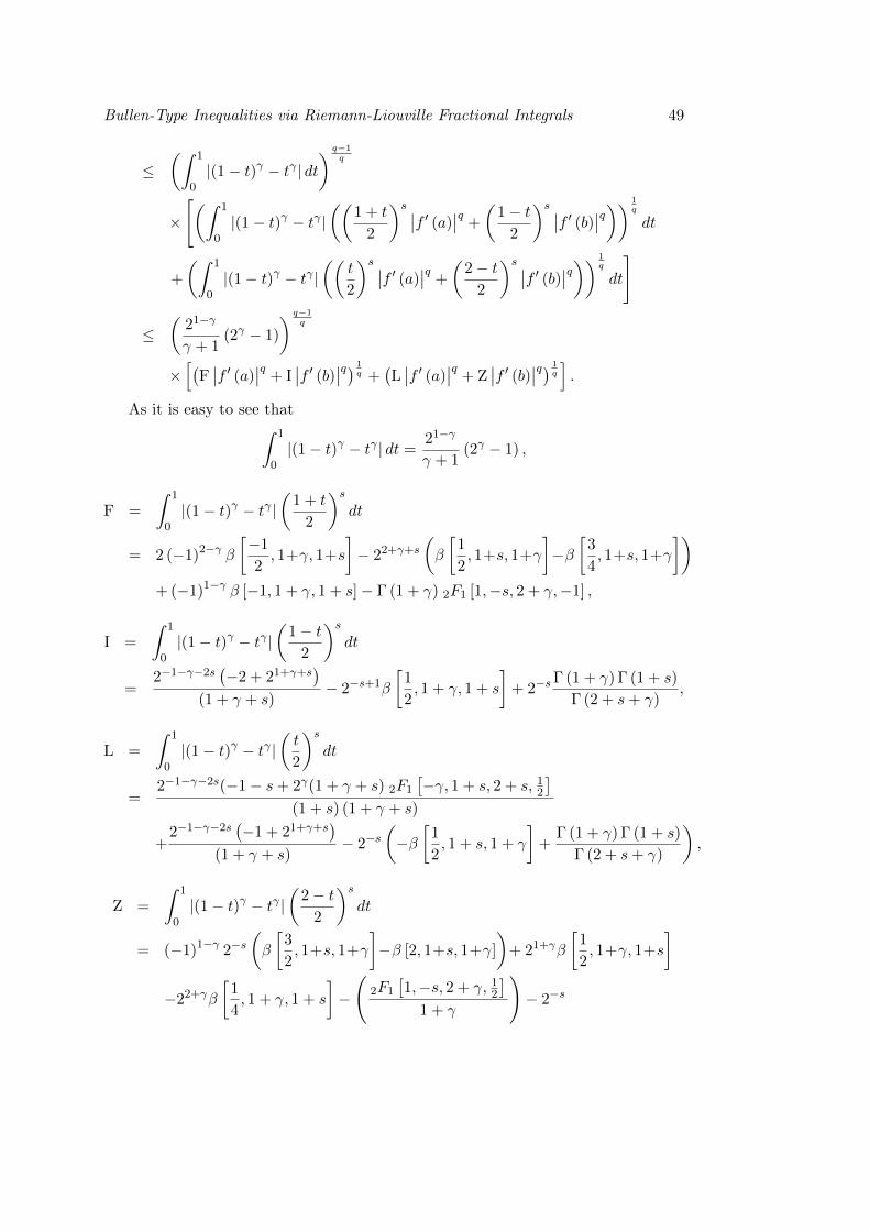
≤(
21−γ
γ + 1(2γ − 1)
) q−1q
×[(
F∣∣f ′ (a)
∣∣q + I∣∣f ′ (b)∣∣q) 1
q +(L∣∣f ′ (a)
∣∣q + Z∣∣f ′ (b)∣∣q) 1
q
].
As it is easy to see that∫ 1
0|(1− t)γ − tγ | dt =
21−γ
γ + 1(2γ − 1) ,
F =
∫ 1
0|(1− t)γ − tγ |
(1 + t
2
)sdt
= 2 (−1)2−γ β
[−1
2, 1+γ, 1+s
]− 22+γ+s
(β
[1
2, 1+s, 1+γ
]−β
[3
4, 1+s, 1+γ
])+ (−1)1−γ β [−1, 1 + γ, 1 + s]− Γ (1 + γ) 2F1 [1,−s, 2 + γ,−1] ,
I =
∫ 1
0|(1− t)γ − tγ |
(1− t
2
)sdt
=2−1−γ−2s
(−2 + 21+γ+s
)(1 + γ + s)
− 2−s+1β
[1
2, 1 + γ, 1 + s
]+ 2−s
Γ (1 + γ) Γ (1 + s)
Γ (2 + s+ γ),
L =
∫ 1
0|(1− t)γ − tγ |
(t
2
)sdt
=2−1−γ−2s(−1− s+ 2γ(1 + γ + s) 2F1
[−γ, 1 + s, 2 + s, 12
](1 + s) (1 + γ + s)
+2−1−γ−2s
(−1 + 21+γ+s
)(1 + γ + s)
− 2−s(−β[
1
2, 1 + s, 1 + γ
]+
Γ (1 + γ) Γ (1 + s)
Γ (2 + s+ γ)
),
Z =
∫ 1
0|(1− t)γ − tγ |
(2− t
2
)sdt
= (−1)1−γ 2−s(β
[3
2, 1+s, 1+γ
]−β [2, 1+s, 1+γ]
)+ 21+γβ
[1
2, 1+γ, 1+s
]−22+γβ
[1
4, 1 + γ, 1 + s
]−
(2F1
[1,−s, 2 + γ, 12
]1 + γ
)− 2−s
50 Musa Cakmak
×
((−1)−γ 2−1−s
(31+s 2F1
[−γ, 1+s, 2+s, 32
]−41+s 2F1 [−γ, 1+s, 2+s, 2]
)1+s
).
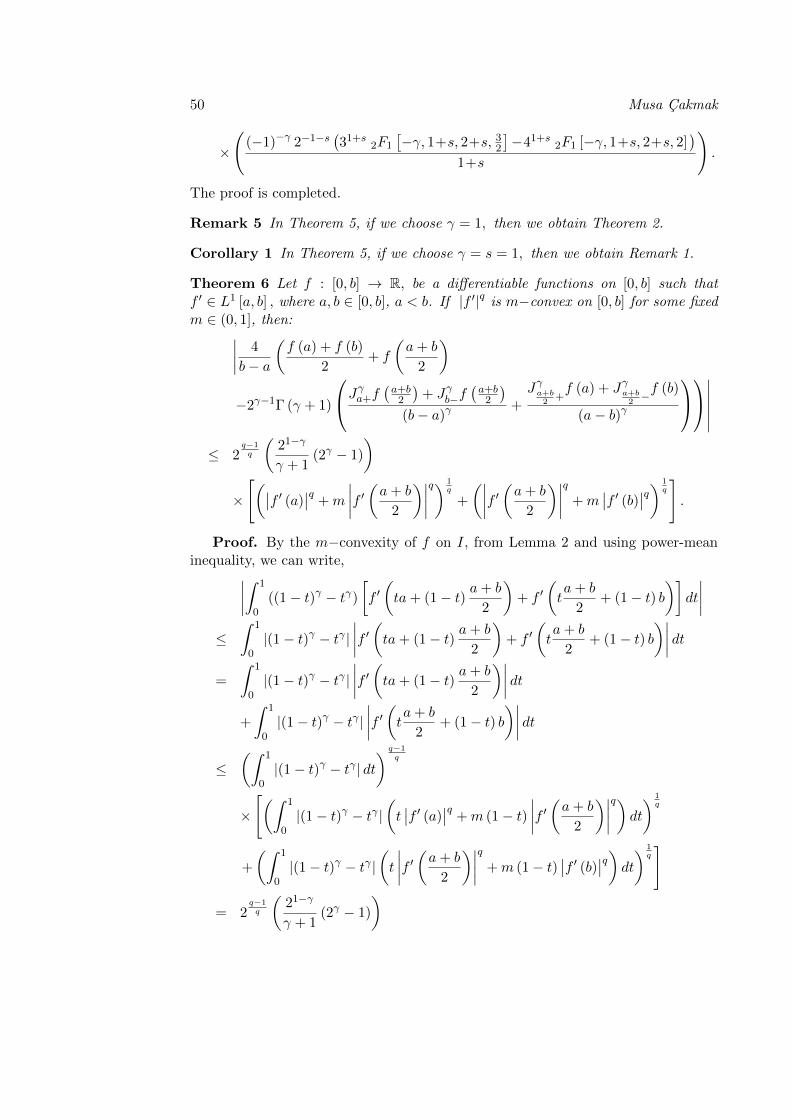
The proof is completed.
Remark 5 In Theorem 5, if we choose γ = 1, then we obtain Theorem 2.
Corollary 1 In Theorem 5, if we choose γ = s = 1, then we obtain Remark 1.
Theorem 6 Let f : [0, b] → R, be a differentiable functions on [0, b] such thatf ′ ∈ L1 [a, b] , where a, b ∈ [0, b], a < b. If |f ′|q is m−convex on [0, b] for some fixedm ∈ (0, 1], then:∣∣∣∣ 4
b− a
(f (a) + f (b)
2+ f
(a+ b
2
)
−2γ−1Γ (γ + 1)
Jγa+f (a+b2 )+ Jγb−f(a+b2
)(b− a)γ
+Jγa+b
2+f (a) + Jγa+b
2−f (b)
(a− b)γ
∣∣∣∣∣∣≤ 2
q−1q
(21−γ
γ + 1(2γ − 1)
)×
[(∣∣f ′ (a)∣∣q +m
∣∣∣∣f ′(a+ b
2
)∣∣∣∣q) 1q
+
(∣∣∣∣f ′(a+ b
2
)∣∣∣∣q +m∣∣f ′ (b)∣∣q) 1
q
].
Proof. By the m−convexity of f on I, from Lemma 2 and using power-meaninequality, we can write,∣∣∣∣∫ 1
0((1− t)γ − tγ)
[f ′(ta+ (1− t) a+ b
2
)+ f ′
(ta+ b
2+ (1− t) b
)]dt
∣∣∣∣≤
∫ 1
0|(1− t)γ − tγ |
∣∣∣∣f ′(ta+ (1− t) a+ b
2
)+ f ′
(ta+ b
2+ (1− t) b
)∣∣∣∣ dt=
∫ 1
0|(1− t)γ − tγ |
∣∣∣∣f ′(ta+ (1− t) a+ b
2
)∣∣∣∣ dt+
∫ 1
0|(1− t)γ − tγ |
∣∣∣∣f ′(ta+ b
2+ (1− t) b
)∣∣∣∣ dt≤
(∫ 1
0|(1− t)γ − tγ | dt
) q−1q
×
[(∫ 1
0|(1− t)γ − tγ |
(t∣∣f ′ (a)
∣∣q +m (1− t)∣∣∣∣f ′(a+ b
2
)∣∣∣∣q) dt)1q
+
(∫ 1
0|(1− t)γ − tγ |
(t
∣∣∣∣f ′(a+ b
2
)∣∣∣∣q +m (1− t)∣∣f ′ (b)∣∣q) dt) 1
q
]
= 2q−1q
(21−γ
γ + 1(2γ − 1)
)
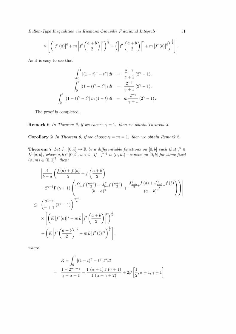
Bullen-Type Inequalities via Riemann-Liouville Fractional Integrals 51
×
[(∣∣f ′ (a)∣∣q +m
∣∣∣∣f ′(a+ b
2
)∣∣∣∣q) 1q
+
(∣∣∣∣f ′(a+ b
2
)∣∣∣∣q +m∣∣f ′ (b)∣∣q) 1
q
].
As it is easy to see that ∫ 1
0|(1− t)γ − tγ | dt =
21−γ
γ + 1(2γ − 1) ,∫ 1
0|(1− t)γ − tγ | tdt =
2−γ
γ + 1(2γ − 1) ,∫ 1
0|(1− t)γ − tγ |m (1− t) dt = m
2−γ
γ + 1(2γ − 1) .
The proof is completed.
Remark 6 In Theorem 6, if we choose γ = 1, then we obtain Theorem 3.
Corollary 2 In Theorem 6, if we choose γ = m = 1, then we obtain Remark 2.
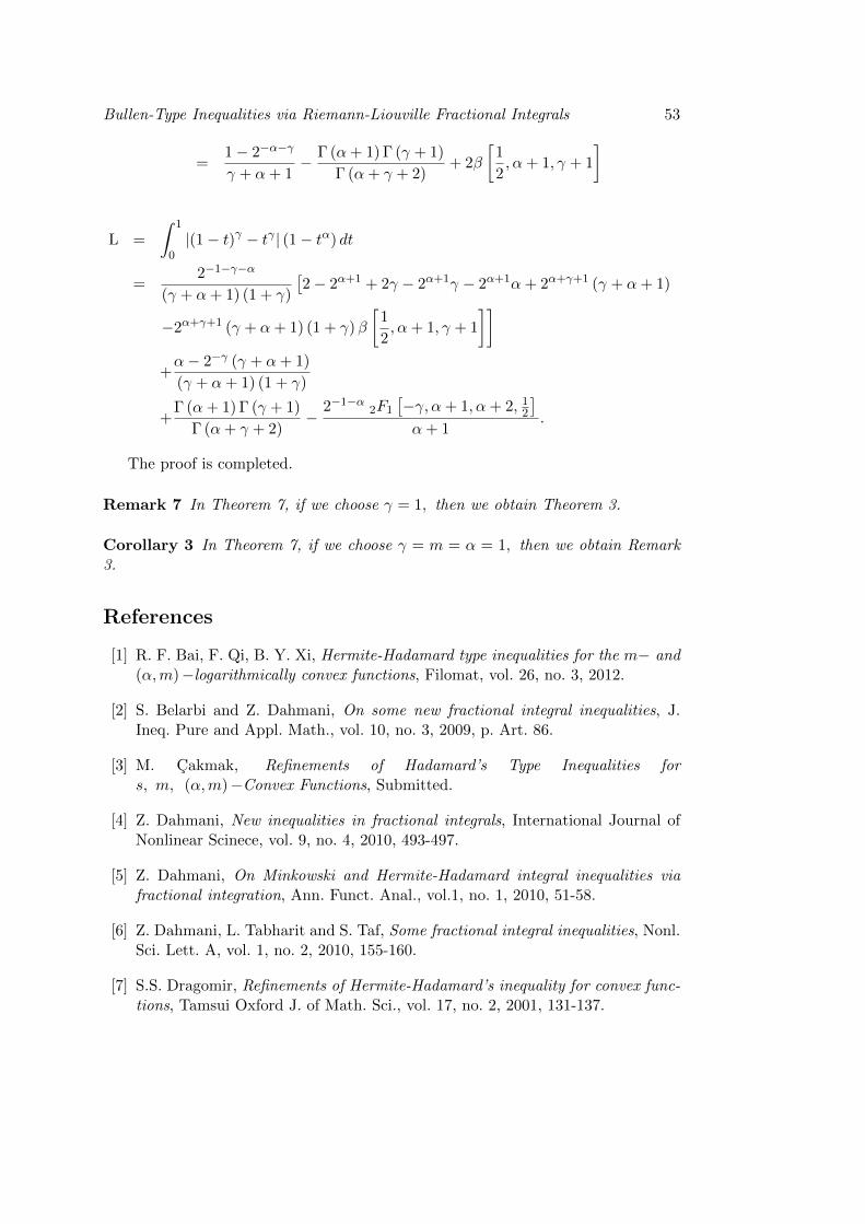
Theorem 7 Let f : [0, b] → R be a differentiable functions on [0, b] such that f ′ ∈L1 [a, b] , where a, b ∈ [0, b], a < b. If |f ′|q is (α,m)−convex on [0, b] for some fixed(α,m) ∈ (0, 1]2, then:∣∣∣∣ 4
b− a
(f (a) + f (b)
2+ f
(a+ b
2
)
−2γ−1Γ (γ + 1)
Jγa+f (a+b2 )+ Jγb−f(a+b2
)(b− a)γ
+Jγa+b
2+f (a) + Jγa+b
2−f (b)
(a− b)γ
∣∣∣∣∣∣≤
(21−γ
γ + 1(2γ − 1)
) q−1q
×
[(K∣∣f ′ (a)
∣∣q +mL
∣∣∣∣f ′(a+ b
2
)∣∣∣∣q) 1q
+
(K
∣∣∣∣f ′(a+ b
2
)∣∣∣∣q +mL∣∣f ′ (b)∣∣q) 1
q
].
where
K =
∫ 1
0|(1− t)γ − tγ | tαdt
=1− 2−α−γ
γ + α+ 1− Γ (α+ 1) Γ (γ + 1)
Γ (α+ γ + 2)+ 2β
[1
2, α+ 1, γ + 1
]
52 Musa Cakmak
L =
∫ 1
0|(1− t)γ − tγ | (1− tα) dt
=2−1−γ−α
(γ + α+ 1) (1 + γ)
[2− 2α+1 + 2γ − 2α+1γ − 2α+1α+ 2α+γ+1 (γ + α+ 1)
−2α+γ+1 (γ + α+ 1) (1 + γ)β
[1
2, α+ 1, γ + 1
]]+α− 2−γ (γ + α+ 1)
(γ + α+ 1) (1 + γ)
+Γ (α+ 1) Γ (γ + 1)
Γ (α+ γ + 2)−
2−1−α 2F1
[−γ, α+ 1, α+ 2, 12
]α+ 1
.
Proof. By the (α,m)−convexity of f on I, from Lemma 2 and using power-mean inequality, we can write,∣∣∣∣∫ 1
0((1− t)γ − tγ)
[f ′(ta+ (1− t) a+ b
2
)+ f ′
(ta+ b
2+ (1− t) b
)]dt
∣∣∣∣≤
∫ 1
0|(1− t)γ − tγ |
∣∣∣∣f ′ta+ (1− t) a+ b
2
∣∣∣∣ dt+
∫ 1
0((1− t)γ − tγ)
∣∣∣∣f ′(ta+ b
2+ (1− t) b
)∣∣∣∣ dt≤
(∫ 1
0|(1− t)γ − tγ | dt
) q−1q
×
[(∫ 1
0|(1− t)γ − tγ |
(tα∣∣f ′ (a)
∣∣q +m (1− tα)
∣∣∣∣f ′(a+ b
2
)∣∣∣∣q) dt)1q
+
(∫ 1
0|(1− t)γ − tγ |
(tα∣∣∣∣f ′(a+ b
2
)∣∣∣∣q +m (1− tα)∣∣f ′ (b)∣∣q) dt) 1
q
]
=
(21−γ
γ + 1(2γ − 1)
) q−1q
×
[(K∣∣f ′ (a)
∣∣q +mL
∣∣∣∣f ′(a+ b
2
)∣∣∣∣q) 1q
+
(K
∣∣∣∣f ′(a+ b
2
)∣∣∣∣q +mL∣∣f ′ (b)∣∣q) 1
q
].
As it is easy to see that ∫ 1
0|(1− t)γ − tγ | dt =
21−γ
γ + 1(2γ − 1) ,
K =
∫ 1
0|(1− t)γ − tγ | tαdt
Bullen-Type Inequalities via Riemann-Liouville Fractional Integrals 53
=1− 2−α−γ
γ + α+ 1− Γ (α+ 1) Γ (γ + 1)
Γ (α+ γ + 2)+ 2β
[1
2, α+ 1, γ + 1
]
L =
∫ 1
0|(1− t)γ − tγ | (1− tα) dt
=2−1−γ−α
(γ + α+ 1) (1 + γ)
[2− 2α+1 + 2γ − 2α+1γ − 2α+1α+ 2α+γ+1 (γ + α+ 1)
−2α+γ+1 (γ + α+ 1) (1 + γ)β
[1
2, α+ 1, γ + 1
]]+α− 2−γ (γ + α+ 1)
(γ + α+ 1) (1 + γ)
+Γ (α+ 1) Γ (γ + 1)
Γ (α+ γ + 2)−
2−1−α 2F1
[−γ, α+ 1, α+ 2, 12
]α+ 1
.
The proof is completed.
Remark 7 In Theorem 7, if we choose γ = 1, then we obtain Theorem 3.
Corollary 3 In Theorem 7, if we choose γ = m = α = 1, then we obtain Remark3.
References
[1] R. F. Bai, F. Qi, B. Y. Xi, Hermite-Hadamard type inequalities for the m− and(α,m)−logarithmically convex functions, Filomat, vol. 26, no. 3, 2012.
[2] S. Belarbi and Z. Dahmani, On some new fractional integral inequalities, J.Ineq. Pure and Appl. Math., vol. 10, no. 3, 2009, p. Art. 86.
[3] M. Cakmak, Refinements of Hadamard’s Type Inequalities fors, m, (α,m)−Convex Functions, Submitted.
[4] Z. Dahmani, New inequalities in fractional integrals, International Journal ofNonlinear Scinece, vol. 9, no. 4, 2010, 493-497.
[5] Z. Dahmani, On Minkowski and Hermite-Hadamard integral inequalities viafractional integration, Ann. Funct. Anal., vol.1, no. 1, 2010, 51-58.
[6] Z. Dahmani, L. Tabharit and S. Taf, Some fractional integral inequalities, Nonl.Sci. Lett. A, vol. 1, no. 2, 2010, 155-160.
[7] S.S. Dragomir, Refinements of Hermite-Hadamard’s inequality for convex func-tions, Tamsui Oxford J. of Math. Sci., vol. 17, no. 2, 2001, 131-137.
54 Musa Cakmak
[8] S.S. Dragomir, R. P. Agarwal, Two Inequalities for Differentiable Mappingsand Applications to Special Means of Real Nubbers and to Trapezoidal Formula,Appl. Math. Lett., vol. 11, no. 5, 1998, 91-95.
[9] S.S. Dragomir, C. E. M. Pearce, Selected Topic on Hermite- Hadamard Inequal-ities and Applications, Melbourne and Adelaide, December, 2000.
[10] S.S. Dragomir, S. Fitzpatricks, The Hadamard’s inequality for s-convex func-tions in the second sense, Demonstratio Math., vol. 32, no. 4, 1999, 687-696.
[11] R. Gorenflo, F. Mainardi, Fractional calculus: integral and differential equationsof fractional order, Springer Verlag, Wien, 1997, 223-276.
[12] H. Hudzik, L. Maligranda, Some remarks on s-convex functions, AequationesMath., 48, 1994, 100-111.
[13] K. T. Kohl, V. H. Moll, The integrals in Gradshteyn and Ryzhik, Part 20:Hypergeometric functions, SCIENTIA Series A: Mathematical Sciences, vol.21, 2011, 43-54.
[14] S. Miller and B. Ross, On introduction to the fractional calculus and fractionaldifferential equations, John Wiley and Sons, USA, vol. 13, no. 2, 1993.
[15] D.S. Mitrinovi, J. Peari, A.M. Fink, Classical and New Inequalities in Analysis,KluwerAcademic, Dordrecht, 1993.
[16] C.E.M. Pearce, J. Peari, Inequalities for differentiable mappings with applicationto special means and quadrature formulae, Appl. Math. Lett.,vol. 13, 2000, 51-55.
[17] J.E. Peari, F. Proschan, Y.L Tong, Convex Functions, Partial Orderings, andStatistical Applications, Academic Press Inc., 1992.
[18] I. Podlubni, Fractional differential equations, Academic Press, San Diego, 1999.
[19] M. Z. Sarikaya, E. Set, H. Yaldiz, N. Basak, Hermite-Hadamard’s inequalitiesfor fractional integrals and related fractional inequalities, Mathematical andComputer Modelling, vol. 57, 2013, 2403-2407, doi: 10.1016/j.mcm.2011.12.048.
[20] M. Z. Sarikaya, H. Yaldiz, On weighted Montogomery identities for Riemann-Liouville fractional integrals, Konuralp Journal of Mathematics, vol. 1, no. 1,2013, 48-53.
[21] F. Qi, Z. L. Wei, Q. Yang, Generalizations and refinements of Hermite-Hadamard’s inequality, The Rocky Mountain Journal of Mathematics, vol. 35,no. 1, 2005, 235-251.
[22] G.H. Toader, On a generalisation of the convexity, Mathematica, vol. 30, no.53, 1988, 83-87.
Bullen-Type Inequalities via Riemann-Liouville Fractional Integrals 55
[23] G.H. Toader, Some generalisations of the convexity, Proc. Colloq. Approx. Op-tim, Cluj-Napoca (Romania), 1984, 329-338.
[24] J. Wang, X. Li, M. Feckan, Y. Zhou, Hermite-Hadamard-type inequalities forRiemann-Liouville fractional integrals via two kinds of convexity, ApplicableAnalysis, 2012, 1-13, doi: 10.1080/00036811.2012.727986.
[25] B.-Y. Xi, F. Qi, Some integral inequalities of Hermite-Hadamard type for convexfunctions with applications to means, J. Funct. Spaces Appl., 2012, Article ID980438.
Musa CakmakHatay Mustafa Kemal UniversityYayladagı Vocational School of Social SciencesMustafa Kemal University, Hatay, 31000, Turkey.e-mail: [email protected]

General Mathematics Vol. 26, No. 1-2 (2018), 57–77
Second Order Approximated Semi-Infinite OptimizationProblems 1
Augusta Ratiu, Dorel I. Duca
Abstract
In this paper, for a semi-infinite optimization Problem (P ), second order η-approximated optimization problems (P0,2), (P2,0), (P1,2), (P2,1) and (P2,2) areconstructed . Some connections are established between the optimal solutionsof these problems and optimal solutions of the original Problem (P ).
2010 Mathematics Subject Classification: 90C34, 90C46, 90C59.
Key words and phrases: semi-infinite optimization, optimal solutions,η-approximation, pseudoinvex function, quasi-incave function, second order
approximation.
1 Introduction
We consider the optimization problem:
(P)
min f(x)such that:
x ∈ Xgt(x) ≤ 0, t ∈ Ths(x) = 0, s ∈ S
where X is a subset of Rn, T and S are nonempty index sets, and f : X → R,gt : X → R, (t ∈ T ) and hs : X → R, (s ∈ S) are functions.
If the sets T and S are finite, then the Problem (P ) is a classic optimizationproblem, otherwise the Problem (P ) is a semi-infinite optimization problem withinfinite number of constraints.
1Received 12 May, 2018Accepted for publication (in revised form) 24 July, 2018
57
58 Augusta Ratiu, Dorel I. Duca
The field of semi-infinite programming appeared in 1924, but the name wascoined in 1962 by Kortanek, Cooper and Charnes in the papers (see, [3], [4]). Inrecent years, semi-infinite programming became an active research topic in appliedmathematics, e.g., air pollution control, fuzzy sets, design problems, reverse Cheby-shev approximation, problems of maneuverability of robots (see, [8], [9]). In theliterature, there are many papers (see, [11], [13], [6]), as well as the books (see, [7],[10]), which contain researches for semi-infinite optimization problems.
There are several methods to solve the Problem (P ). One of them might be toattach another optimization problem whose solutions will provide information aboutthe optimal solution of the original problem. Antczak in [1] and [2], approached theissue in this manner introducing the notion of η-approximation. For T and S finites,he constructed a η-approximated optimization problem equivalent with the originalmathematical programming problem and he studied connections between optimalsolutions of the two problems. In [5], Duca and Duca solved this problem in moregeneral conditions.
Let η : X ×X → X be a function, x0 be an interior point of X. If the functionsf : X → R, gt : X → R, (t ∈ T ) and hs : X → R, (s ∈ S) are differentiable at x0,
then we denote by F 〈1〉, G〈1〉t , H
〈1〉s : X → R (t ∈ T, s ∈ S) the functions defined by:
F 〈1〉 (x) := f(x0) +[∇f(x0)
] (η(x, x0)
),
G〈1〉t (x) := gt(x
0) +[∇gt(x0)
] (η(x, x0)
), (t ∈ T ) ,
H〈1〉s (x) := hs(x
0) +[∇hs(x0)
] (η(x, x0)
), (s ∈ S) ,
for all x ∈ X, and if the functions f : X → R, gt : X → R, (t ∈ T ) and hs : X → R,(s ∈ S) are twice differentiable at x0, then we denote by F 〈2〉, G
〈2〉t , H
〈2〉s : X → R
(t ∈ T, s ∈ S) the functions defined by:
F 〈2〉 (x) := f(x0) +[∇f(x0)
] (η(x, x0)
)+
+ 12
⟨η(x, x0),
[∇2f(x0)
] (η(x, x0)
)⟩,
G〈2〉t (x) := gt(x
0) +[∇gt(x0)
] (η(x, x0)
)+
+ 12
⟨η(x, x0),
[∇2gt(x
0)] (η(x, x0)
)⟩≤ 0, (t ∈ T ),
H〈2〉s (x) := hs(x
0) +[∇hs(x0)
] (η(x, x0)
)+
+12
⟨η(x, x0), [∇2hs(x
0)](η(x, x0)
)⟩= 0, (s ∈ S).
Let F 〈0〉 = f , G〈0〉t = gt, H
〈0〉s = hs, (t ∈ T, s ∈ S).
In [12], Ratiu and Duca attached to Problem (P ), the problems: (P1,0), (P0,1)and (P1,1), where (Pj,k), ((j, k) ∈ {(1, 0), (0, 1), (1, 1)}), is the problem:
Semi-Infinite Optimization Problems 59
(Pj,k)
min F 〈j〉 (x)such that:
x ∈ XG
〈k〉t (x) ≤ 0, t ∈ T
H〈k〉s (x) = 0, s ∈ S
called (j, k)-η approximated optimization problem, and some connections betweenthe optimal solutions of their are given.
The goal of this paper is to attach to Problem (P ), the problems: (P2,0), (P0,2),(P1,2), (P2,1) and (P2,2), where (Pj,k), ((j, k) ∈ {(2, 0), (0, 2), (1, 2), (2, 1),(2, 2)}), is the problem:
(Pj,k)
min F 〈j〉 (x)such that:
x ∈ XG
〈k〉t (x) ≤ 0, t ∈ T
H〈k〉s (x) = 0, s ∈ S
called (j, k)-η approximated optimization problem.In what follows, we denote by:
F0 :={x ∈ X : G
〈0〉t (x) ≤ 0, (t ∈ T ) , H〈0〉
s (x) = 0, (s ∈ S)},
F1 :={x ∈ X : G
〈1〉t (x) ≤ 0, (t ∈ T ), H〈1〉
s (x) = 0, (s ∈ S)},
andF2 :=
{x ∈ X : G
〈2〉t (x) ≤ 0, (t ∈ T ) , H〈2〉
s (x) = 0, (s ∈ S)}.
Let’s remark that if F(P ) denote the set of all feasible solution of Problem (P ),then F0 = F(P ) = F(P1,0) = F(P2,0), F1 = F(P0,1) = F(P1,1) = F(P2,1) andF2 = F(P0,2) = F(P1,2) = F(P2,2).
After presenting some concepts, in paragraph 3, are given some connections be-tween the optimal solutions of Problem (P ) and approximated (P0,2), (P2,0), (P1,2),(P2,1), (P2,2).
2 Definitions and preliminary results
Definition 1 Let X be a nonempty subset of Rn, x0 be an interior point of X, f :X → R be a differentiable function at x0 and η : X×X → X be a function. We saythat:
(a) the function f is invex at x0 with respect to (w.r.t.) η if, for all x ∈ X,
f(x)− f(x0) ≥ [∇f(x0)](η(x, x0)),
60 Augusta Ratiu, Dorel I. Duca
or, equivalently,f (x) ≥ F 〈1〉 (x) ,
(b) the function f is incave at x0 w.r.t. η if (−f) is invex at x0 w.r.t. η,(c) the function f is avex at x0 w.r.t. η if f is both invex and incave at x0 w.r.t.
η,(d) the function f is pseudoinvex at x0 w.r.t. η if, for all x ∈ X,
[∇f(x0)](η(x, x0)) ≥ 0⇒ f(x)− f(x0) ≥ 0,
or, equivalently,F 〈1〉 (x)− f
(x0)≥ 0⇒ f(x)− f(x0) ≥ 0,
(e) the function f is quasiincave at x0 w.r.t. η if, for all x ∈ X,
f(x)− f(x0) ≥ 0⇒ [∇f(x0)](η(x, x0)) ≥ 0,
or, equivalently,f(x)− f(x0) ≥ 0⇒ F 〈1〉 (x)− f(x0) ≥ 0.
Definition 2 Let X be a nonempty subset of Rn, x0 be an interior point of X, f :X → R be a twice differentiable function at x0 and η : X ×X → X be a function.We say that:
(a) the function f is second order invex at x0 w.r.t. η if, for all x ∈ X,
f(x)− f(x0) ≥[∇f(x0)
] (η(x, x0)
)+
+ 12
⟨η(x, x0),
[∇2f(x0)
] (η(x, x0)
)⟩,
or, equivalently,f(x) ≥ F 〈2〉(x),
(b) the function f is second order incave at x0 w.r.t. η if, for all x ∈ X,
f(x)− f(x0) ≤[∇f(x0)
] (η(x, x0)
)+
+ 12
⟨η(x, x0),
[∇2f(x0)
] (η(x, x0)
)⟩,
or, equivalently,f(x) ≤ F 〈2〉(x),
(c) the function f is second order avex at x0 w.r.t. η if
f(x) = F 〈2〉(x), for all x ∈ X,
(d) the function f is second order pseudoinvex at x0 w.r.t. η if, for all x ∈ X,
[∇f(x0)](η(x, x0)) + 12
⟨η(x, x0),
[∇2f(x0)
] (η(x, x0)
)⟩≥ 0 =⇒
=⇒ f(x)− f(x0) ≥ 0,
or, equivalently,
F 〈2〉(x)− f(x0) ≥ 0 =⇒ f(x)− f(x0) ≥ 0,
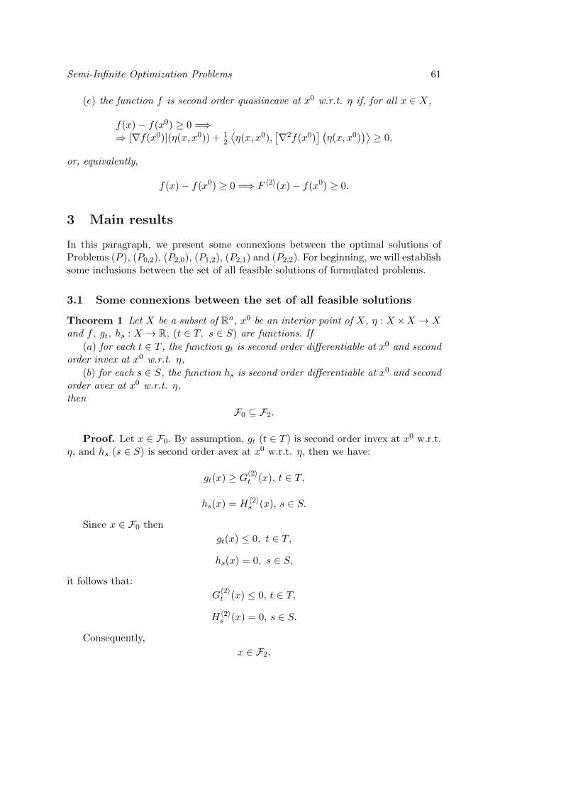
Semi-Infinite Optimization Problems 61
(e) the function f is second order quasiincave at x0 w.r.t. η if, for all x ∈ X,
f(x)− f(x0) ≥ 0 =⇒⇒ [∇f(x0)](η(x, x0)) + 1
2
⟨η(x, x0),
[∇2f(x0)
] (η(x, x0)
)⟩≥ 0,
or, equivalently,
f(x)− f(x0) ≥ 0 =⇒ F 〈2〉(x)− f(x0) ≥ 0.
3 Main results
In this paragraph, we present some connexions between the optimal solutions ofProblems (P ), (P0,2), (P2,0), (P1,2), (P2,1) and (P2,2). For beginning, we will establishsome inclusions between the set of all feasible solutions of formulated problems.
3.1 Some connexions between the set of all feasible solutions
Theorem 1 Let X be a subset of Rn, x0 be an interior point of X, η : X ×X → Xand f , gt, hs : X → R, (t ∈ T, s ∈ S) are functions. If
(a) for each t ∈ T , the function gt is second order differentiable at x0 and secondorder invex at x0 w.r.t. η,
(b) for each s ∈ S, the function hs is second order differentiable at x0 and secondorder avex at x0 w.r.t. η,then
F0 ⊆ F2.
Proof. Let x ∈ F0. By assumption, gt (t ∈ T ) is second order invex at x0 w.r.t.η, and hs (s ∈ S) is second order avex at x0 w.r.t. η, then we have:
gt(x) ≥ G〈2〉t (x), t ∈ T,
hs(x) = H〈2〉s (x), s ∈ S.
Since x ∈ F0 then
gt(x) ≤ 0, t ∈ T,
hs(x) = 0, s ∈ S,
it follows that:
G〈2〉t (x) ≤ 0, t ∈ T,
H〈2〉s (x) = 0, s ∈ S.
Consequently,
x ∈ F2.
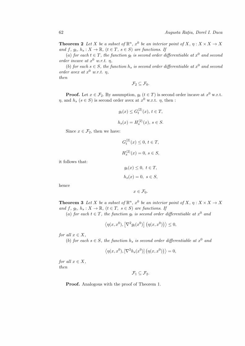
62 Augusta Ratiu, Dorel I. Duca
Theorem 2 Let X be a subset of Rn, x0 be an interior point of X, η : X ×X → Xand f , gt, hs : X → R, (t ∈ T , s ∈ S) are functions. If
(a) for each t ∈ T , the function gt is second order differentiable at x0 and secondorder incave at x0 w.r.t. η,
(b) for each s ∈ S, the function hs is second order differentiable at x0 and secondorder avex at x0 w.r.t. η,then
F2 ⊆ F0.
Proof. Let x ∈ F2. By assumption, gt (t ∈ T ) is second order incave at x0 w.r.t.η, and hs (s ∈ S) is second order avex at x0 w.r.t. η, then :
gt(x) ≤ G〈2〉t (x), t ∈ T,
hs(x) = H〈2〉s (x), s ∈ S.
Since x ∈ F2, then we have:
G〈2〉t (x) ≤ 0, t ∈ T,
H〈2〉s (x) = 0, s ∈ S,
it follows that:
gt(x) ≤ 0, t ∈ T,
hs(x) = 0, s ∈ S,
hence
x ∈ F0.
Theorem 3 Let X be a subset of Rn, x0 be an interior point of X, η : X ×X → Xand f , gt, hs : X → R, (t ∈ T, s ∈ S) are functions. If
(a) for each t ∈ T , the function gt is second order differentiable at x0 and⟨η(x, x0),
[∇2gt(x
0)] (η(x, x0)
)⟩≤ 0,
for all x ∈ X,
(b) for each s ∈ S, the function hs is second order differentiable at x0 and⟨η(x, x0), [∇2hs(x
0)](η(x, x0)
)⟩= 0,
for all x ∈ X,then
F1 ⊆ F2.
Proof. Analogous with the proof of Theorem 1.
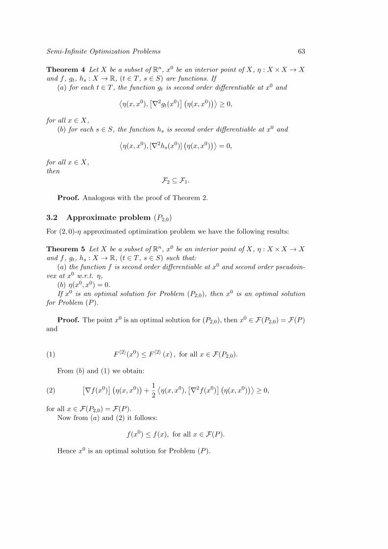
Semi-Infinite Optimization Problems 63
Theorem 4 Let X be a subset of Rn, x0 be an interior point of X, η : X ×X → Xand f , gt, hs : X → R, (t ∈ T , s ∈ S) are functions. If
(a) for each t ∈ T , the function gt is second order differentiable at x0 and⟨η(x, x0),
[∇2gt(x
0)] (η(x, x0)
)⟩≥ 0,
for all x ∈ X,
(b) for each s ∈ S, the function hs is second order differentiable at x0 and⟨η(x, x0), [∇2hs(x
0)](η(x, x0)
)⟩= 0,
for all x ∈ X,then
F2 ⊆ F1.
Proof. Analogous with the proof of Theorem 2.
3.2 Approximate problem (P2,0)
For (2, 0)-η approximated optimization problem we have the following results:
Theorem 5 Let X be a subset of Rn, x0 be an interior point of X, η : X ×X → Xand f , gt, hs : X → R, (t ∈ T , s ∈ S) such that:
(a) the function f is second order differentiable at x0 and second order pseudoin-vex at x0 w.r.t. η,
(b) η(x0, x0) = 0.
If x0 is an optimal solution for Problem (P2,0), then x0 is an optimal solutionfor Problem (P ).
Proof. The point x0 is an optimal solution for (P2,0), then x0 ∈ F(P2,0) = F(P )and
(1) F 〈2〉(x0) ≤ F 〈2〉 (x) , for all x ∈ F(P2,0).
From (b) and (1) we obtain:
(2)[∇f(x0)
] (η(x, x0)
)+
1
2
⟨η(x, x0),
[∇2f(x0)
] (η(x, x0)
)⟩≥ 0,
for all x ∈ F(P2,0) = F(P ).
Now from (a) and (2) it follows:
f(x0) ≤ f(x), for all x ∈ F(P ).
Hence x0 is an optimal solution for Problem (P ).
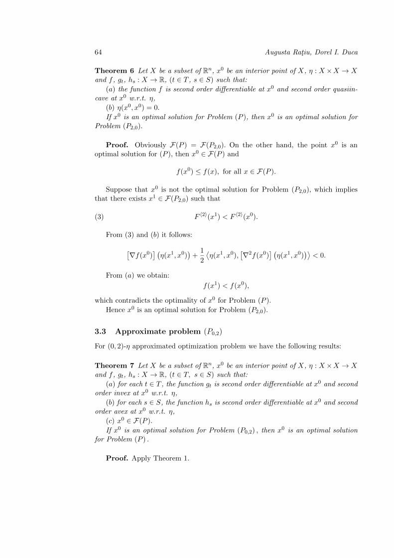
64 Augusta Ratiu, Dorel I. Duca
Theorem 6 Let X be a subset of Rn, x0 be an interior point of X, η : X ×X → Xand f , gt, hs : X → R, (t ∈ T , s ∈ S) such that:
(a) the function f is second order differentiable at x0 and second order quasiin-cave at x0 w.r.t. η,
(b) η(x0, x0) = 0.
If x0 is an optimal solution for Problem (P ), then x0 is an optimal solution forProblem (P2,0).
Proof. Obviously F(P ) = F(P2,0). On the other hand, the point x0 is anoptimal solution for (P ), then x0 ∈ F(P ) and
f(x0) ≤ f(x), for all x ∈ F(P ).
Suppose that x0 is not the optimal solution for Problem (P2,0), which impliesthat there exists x1 ∈ F(P2,0) such that
(3) F 〈2〉(x1) < F 〈2〉(x0).
From (3) and (b) it follows:
[∇f(x0)
] (η(x1, x0)
)+
1
2
⟨η(x1, x0),
[∇2f(x0)
] (η(x1, x0)
)⟩< 0.
From (a) we obtain:
f(x1) < f(x0),
which contradicts the optimality of x0 for Problem (P ).
Hence x0 is an optimal solution for Problem (P2,0).
3.3 Approximate problem (P0,2)
For (0, 2)-η approximated optimization problem we have the following results:
Theorem 7 Let X be a subset of Rn, x0 be an interior point of X, η : X ×X → Xand f , gt, hs : X → R, (t ∈ T, s ∈ S) such that:
(a) for each t ∈ T , the function gt is second order differentiable at x0 and secondorder invex at x0 w.r.t. η,
(b) for each s ∈ S, the function hs is second order differentiable at x0 and secondorder avex at x0 w.r.t. η,
(c) x0 ∈ F(P ).
If x0 is an optimal solution for Problem (P0,2) , then x0 is an optimal solutionfor Problem (P ) .
Proof. Apply Theorem 1.
Semi-Infinite Optimization Problems 65
Theorem 8 Let X be a subset of Rn, x0 be an interior point of X, η : X ×X → Xand f , gt, hs : X → R, (t ∈ T , s ∈ S) such that:
(a) for each t ∈ T , the function gt is second order differentiable at x0 and secondorder incave at x0 w.r.t. η,
(b) for each s ∈ S, the function hs is second order differentiable at x0 and secondorder avex at x0 w.r.t. η,
(c) x0 ∈ F(P0,2).If x0 is an optimal solution for Problem (P ) , then x0 is an optimal solution for
Problem (P0,2) .
Proof. Apply Theorem 2.
3.4 Approximate problem (P1,2)
For (1, 2)-η approximated optimization problem we have the following results:
Theorem 9 Let X be a subset of Rn, x0 be an interior point of X, η : X ×X → Xand f , gt, hs : X → R, (t ∈ T , s ∈ S) such that:
(a) the function f is differentiable at x0 and pseudoinvex at x0 w.r.t. η,(b) for each t ∈ T , the function gt is second order differentiable at x0 and second
order invex at x0 w.r.t. η,(c) for each s ∈ S, the function hs is second order differentiable at x0 and second
order avex at x0 w.r.t. η,(d) x0 ∈ F(P ),(e) η(x0, x0) = 0.If x0 is an optimal solution for Problem (P1,2), then x0 is an optimal solution
for Problem (P ).
Proof. The point x0 is an optimal solution for (P1,2), then we have:
(4) F 〈1〉(x0) ≤ F 〈1〉(x), for all x ∈ F(P1,2).
By Theorem 1, we have:F(P ) ⊆ F(P1,2).
From (e) and (4) we obtain:
(5)[∇f(x0)
] (η(x, x0)
)≥ 0, for all x ∈ F(P1,2).
Now from (a) and (5) it follows:
f(x0) ≤ f(x), for all x ∈ F(P1,2),
then, from (d),f(x0) ≤ f(x), for all x ∈ F(P ).
Hence x0 is an optimal solution for Problem (P ).
66 Augusta Ratiu, Dorel I. Duca
Theorem 10 Let X be a subset of Rn, x0 be an interior point of X, η : X×X → Xand f , gt, hs : X → R, (t ∈ T , s ∈ S) such that:
(a) the function f is differentiable at x0 and quasi-incave at x0 w.r.t. η,(b) for each t ∈ T , the function gt is second order differentiable at x0 and second
order incave at x0 w.r.t. η,(c) for each s ∈ S, the function hs is second order differentiable at x0 and second
order avex at x0 w.r.t. η,(d) x0 ∈ F(P1,2),(e) η(x0, x0) = 0.If x0 is an optimal solution for Problem (P ), then x0 is an optimal solution for
Problem (P1,2).
Proof. The point x0 is an optimal solution for (P ), then we have:
(6) f(x0) ≤ f(x), for all x ∈ F(P ).
On the other hand, by Theorem 2
F(P1,2) ⊆ F(P ).
Now from (6) and (a) it follows:[∇f(x0)
] (η(x, x0)
)≥ 0, for all x ∈ F(P ),
hence [∇f(x0)
] (η(x, x0)
)≥ 0, for all x ∈ F(P1,2).
Consequently,F 〈1〉(x0) ≤ F 〈1〉(x), for all x ∈ F(P1,2).
Hence x0 is an optimal solution for Problem (P1,2).
3.5 Approximate problem (P2,1)
For (2, 1)-η approximated optimization problem we have the following results:
Theorem 11 Let X be a subset of Rn, x0 be an interior point of X, η : X×X → Xand f , gt, hs : X → R, (t ∈ T , s ∈ S) such that:
(a) the function f is second order differentiable at x0 and second order pseudoin-vex at x0 w.r.t. η,
(b) for each t ∈ T , the function gt is differentiable at x0 and invex at x0 w.r.t.η,
(c) for each s ∈ S, the function hs is differentiable at x0 and avex at x0 w.r.t.η,
(d) x0 ∈ F(P ),(e) η(x0, x0) = 0.If x0 is an optimal solution for Problem (P2,1), then x0 is an optimal solution
for Problem (P ).
Semi-Infinite Optimization Problems 67
Proof. The point x0 is an optimal solution for (P2,1), then we have
(7) F 〈2〉(x0) ≤ F 〈2〉(x), for all x ∈ F(P2,1).
From (7) and (e) we obtain:[∇f(x0)
] (η(x, x0)
)+
1
2
⟨η(x, x0),
[∇2f(x0)
] (η(x, x0)
)⟩≥ 0, for all x ∈ F(P2,1).
By assumption (a) we have:
f(x0) ≤ f(x), for all x ∈ F(P2,1).
From (d), we deduce:
f(x0) ≤ f(x), for all x ∈ F(P ).
Hence x0 is an optimal solution for Problem (P ).
Theorem 12 Let X be a subset of Rn, x0 be an interior point of X, η : X×X → Xand f , gt, hs : X → R, (t ∈ T , s ∈ S) such that:
(a) the function f is second order differentiable at x0 and second order quasiin-cave at x0 w.r.t. η,
(b) for each t ∈ T , the function gt is differentiable at x0 and incave at x0 w.r.t.η,
(c) for each s ∈ S, the function hs is differentiable at x0 and avex at x0 w.r.t.η,
(d) x0 ∈ F(P2,1),(e) η(x0, x0) = 0.If x0 is an optimal solution for Problem (P ), then x0 is an optimal solution for
Problem (P2,1).
Proof. The point x0 is an optimal solution for Problem (P ), we have:
f(x0) ≤ f(x), for all x ∈ F(P ).
On the other hand, from (a) and (d),
(8)[∇f(x0)
] (η(x, x0)
)+
1
2
⟨η(x, x0),
[∇2f(x0)
] (η(x, x0)
)⟩≥ 0,
for all x ∈ F(P ), and
F 〈2〉(x0) ≤ F 〈2〉(x), for all x ∈ F(P2,1).
We obtain:
(9)[∇f(x0)
] (η(x, x0)
)+
1
2
⟨η(x, x0),
[∇2f(x0)
] (η(x, x0)
)⟩≥ 0,
for all x ∈ F(P2,1).From (8) and (9), we deduce that x0 is an optimal solution for Problem (P2,1).
68 Augusta Ratiu, Dorel I. Duca
3.6 Approximate problem (P2,2)
For (2, 2)-η approximated optimization problem we have the following results:
Theorem 13 Let X be a subset of Rn, x0 be an interior point of X, η : X×X → Xand f , gt, hs : X → R, (t ∈ T, s ∈ S) such that:
(a) the function f is second order differentiable at x0 and second order pseudoin-vex at x0 w.r.t. η,
(b) for each t ∈ T , the function gt is second order differentiable at x0 and secondorder invex at x0 w.r.t. η,
(c) for each s ∈ S, the function hs is second order differentiable at x0 and secondorder avex at x0 w.r.t. η,
(d) η(x0, x0) = 0,
(e) x0 ∈ F(P ).
If x0 is an optimal solution for Problem (P2,2) , then x0 is an optimal solutionfor Problem (P ) .
Proof. Apply Theorem 1 and Theorem 5.
Theorem 14 Let X be a subset of Rn, x0 be an interior point of X, η : X×X → Xand f , gt, hs : X → R, (t ∈ T , s ∈ S) such that:
(a) the function f is second order differentiable at x0 and second order quasiin-cave at x0 w.r.t. η,
(b) for each t ∈ T , the function gt is second order differentiable at x0 and secondorder incave at x0 w.r.t. η,
(c) for each s ∈ S, the function hs is second order differentiable at x0 and secondorder avex at x0 w.r.t. η,
(d) η(x0, x0) = 0,
(e) x0 ∈ F(P2,2).
If x0 is an optimal solution for Problem (P ) , then x0 is an optimal solution forProblem (P2,2) .
Proof. Apply Theorem 2 and Theorem 6.
3.7 Corollaries
Corollary 1 Let X be a subset of Rn, x0 be an interior point of X, η : X×X → Xand f , gt, hs : X → R, (t ∈ T , s ∈ S) such that:
(a) the function f is second order differentiable at x0, second order pseudoinvexat x0 w.r.t. η and quasiincave at x0 w.r.t. η,
(b) for each t ∈ T , the function gt is second order differentiable at x0 and secondorder incave at x0 w.r.t. η,
(c) for each s ∈ S, the function hs is second order differentiable at x0 and secondorder avex at x0 w.r.t. η,
(d) x0 ∈ F(P1,2),
Semi-Infinite Optimization Problems 69
(e) η(x0, x0) = 0.If x0 is an optimal solution for Problem (P2,0), then x0 is an optimal solution
for Problem (P1,2).
Proof. By Theorem 5, x0 is an optimal solution for Problem (P ) and by Theo-rem 10, x0 is an optimal solution for Problem (P1,2) .
Corollary 2 Let X be a subset of Rn, x0 be an interior point of X, η : X×X → Xand f , gt, hs : X → R, (t ∈ T , s ∈ S) such that:
(a) the function f is second order differentiable at x0, second order quasi-incaveat x0 w.r.t. η and pseudoinvex at x0 w.r.t. η,
(b) for each t ∈ T , the function gt is second order differentiable at x0 and secondorder invex at x0 w.r.t. η,
(c) for each s ∈ S, the function hs is second order differentiable at x0 and secondorder avex at x0 w.r.t. η,
(d) x0 ∈ F(P ),(e) η(x0, x0) = 0.If x0 is an optimal solution for Problem (P1,2), then x0 is an optimal solution
for Problem (P2,0).
Proof. By Theorem 9, x0 is an optimal solution for Problem (P ) and byTheorem 6, x0 is an optimal solution for Problem (P2,0) .
Corollary 3 Let X be a subset of Rn, x0 be an interior point of X, η : X×X → Xand f , gt, hs : X → R, (t ∈ T , s ∈ S) such that:
(a) the function f is second order differentiable at x0, pseudoinvex at x0 w.r.t.η and second order quasiincave at x0 w.r.t. η,
(b) for each t ∈ T , the function gt is second order differentiable at x0, incave atx0 w.r.t. η and second order invex at x0 w.r.t. η
(c) for each s ∈ S, the function hs is second order differentiable at x0, incave atx0 w.r.t. η and second order avex at x0 w.r.t. η,
(d) x0 ∈ F(P ) ∩ F(P2,1),(e) η(x0, x0) = 0.If x0 is an optimal solution for Problem (P1,2), then x0 is an optimal solution
for Problem (P2,1).
Proof. By Theorem 9, x0 is an optimal solution for Problem (P ) , and byTheorem 12, x0 is an optimal solution for Problem (P2,1) .
Corollary 4 Let X be a subset of Rn, x0 be an interior point of X, η : X×X → Xand f , gt, hs : X → R, (t ∈ T , s ∈ S) such that:
(a) the function f is second order differentiable at x0 and second order pseudoin-vex at x0 w.r.t. η and quasi-incave at x0 w.r.t. η,
(b) for each t ∈ T , the function gt is second order differentiable at x0, secondorder incave at x0 w.r.t. η and invex at x0 w.r.t. η,
70 Augusta Ratiu, Dorel I. Duca
(c) for each s ∈ S, the function hs is second order differentiable at x0, secondorder avex at x0 w.r.t. η and avex at x0 w.r.t. η,
(d) x0 ∈ F(P ) ∩ F(P1,2),
(e) η(x0, x0) = 0.
If x0 is an optimal solution for Problem (P2,1), then x0 is an optimal solutionfor Problem (P1,2).
Proof. By Theorem 11, x0 is an optimal solution for Problem (P ) and then byTheorem 10, x0 is an optimal solution for Problem (P1,2) .
Corollary 5 Let X be a subset of Rn, x0 be an interior point of X, η : X×X → Xand f , gt, hs : X → R, (t ∈ T , s ∈ S) such that:
(a) the function f is second order differentiable at x0,
(b) for each t ∈ T , the function gt is differentiable at x0 and invex at x0 w.r.t.η,
(c) for each s ∈ S, the function hs is differentiable at x0 and avex at x0 w.r.t. η,
(d) x0 ∈ F(P2,0).
If x0 is an optimal solution for Problem (P2,1), then x0 is an optimal solutionfor Problem (P2,0).
Proof. The point x0 is an optimal solution for (P2,1), then
F 〈2〉(x0) ≤ F 〈2〉(x), for all x ∈ F(P2,1).
From (d) and F(P2,0) ⊆ F(P2,1), (by Theorem 2 [12]), we have that x0 is anoptimal solution for Problem (P2,0).
Corollary 6 Let X be a subset of Rn, x0 be an interior point of X, η : X×X → Xand f , gt, hs : X → R, (t ∈ T , s ∈ S) such that:
(a) the function f is second order differentiable at x0,
(b) for each t ∈ T , the function gt is differentiable at x0 and incave at x0 w.r.t.η,
(c) for each s ∈ S, the function hs is differentiable at x0 and avex at x0 w.r.t.η,
(d) x0 ∈ F(P2,1),
If x0 is an optimal solution for Problem (P2,0), then x0 is an optimal solutionfor Problem (P2,1).
Proof. The point x0 is an optimal solution for (P2,0), then
(10) F 〈2〉(x0) ≤ F 〈2〉(x), for all x ∈ F(P2,0).
From (d) and F(P2,1) ⊆ F(P2,0), (by Theorem 3 [12]), we have that x0 is anoptimal solution for Problem (P2,1).
Semi-Infinite Optimization Problems 71
Corollary 7 Let X be a subset of Rn, x0 be an interior point of X, η : X×X → Xand f , gt, hs : X → R, (t ∈ T, s ∈ S) such that:
(a) the function f is differentiable at x0 and quasi-incave at x0 w.r.t. η,(b) for each t ∈ T , the function gt is second order differentiable at x0,(c) for each s ∈ S, the function hs is second order differentiable at x0,(d) η(x0, x0) = 0.If x0 is an optimal solution for Problem (P0,2) , then x0 is an optimal solution
for Problem (P1,2) .
Proof. Obviously F(P0,2) = F(P1,2). On the other hand, the point x0 is anoptimal solution for (P0,2), then
(11) f(x0) ≤ f(x), for all x ∈ F(P0,2).
From (11) and (a) it follows:
(12)[∇f(x0)
] (η(x, x0)
)≥ 0, for all x ∈ F(P0,2).
Now from (d) and (12),F 〈1〉(x0) ≤ F 〈1〉(x),
for all x ∈ F(P0,2) = F(P1,2).Hence x0 is an optimal solution for Problem (P1,2).
Corollary 8 Let X be a subset of Rn, x0 be an interior point of X, η : X×X → Xand f , gt, hs : X → R, (t ∈ T , s ∈ S) such that:
(a) the function f is differentiable at x0 and pseudoinvex at x0 w.r.t. η,(b) for each t ∈ T , the function gt is second order differentiable at x0,(c) for each s ∈ S, the function hs is second order differentiable at x0,(d) η(x0, x0) = 0.If x0 is an optimal solution for Problem (P1,2), then x0 is an optimal solution
for Problem (P0,2) .
Proof. Obviously F(P0,2) = F(P1,2). On the other hand, the point x0 is anoptimal solution for (P1,2), then
(13) F 〈1〉(x0) ≤ F 〈1〉(x), for all x ∈ F(P1,2).
From (13) and (d),[∇f(x0)
] (η(x, x0)
)≥ 0, for all x ∈ F(P1,2).
Now from (a) and (13) it follows:
f(x0) ≤ f(x), for all x ∈ F(P0,2) = F(P1,2).
Hence x0 is an optimal solution for Problem (P0,2).
72 Augusta Ratiu, Dorel I. Duca
Corollary 9 Let X be a subset of Rn, x0 be an interior point of X, η : X×X → Xand f , gt, hs : X → R, (t ∈ T , s ∈ S) such that:
(a) the function f is second order differentiable at x0 and second order quasiin-cave at x0 w.r.t. η,
(b) for each t ∈ T , the function gt is second order differentiable at x0 and secondorder invex at x0 w.r.t. η,
(c) for each s ∈ S, the function hs is second order differentiable at x0 and secondorder avex at x0 w.r.t. η,
(d) x0 ∈ F(P ),
(e) η(x0, x0) = 0.
If x0 is an optimal solution for Problem (P0,2), then x0 is an optimal solutionfor Problem (P2,0) .
Proof. By Theorem 7, x0 is an optimal solution for Problem (P ) and then byTheorem 6, x0 is an optimal solution for Problem (P2,0).
Corollary 10 Let X be a subset of Rn, x0 be an interior point of X, η : X×X → Xand f , gt, hs : X → R, (t ∈ T , s ∈ S) such that:
(a) the function f is second order differentiable at x0 and second order pseudoin-vex at x0 w.r.t. η,
(b) for each t ∈ T , the function gt is second order differentiable at x0 and secondorder incave at x0 w.r.t. η,
(c) for each s ∈ S, the function hs is second order differentiable at x0 and secondorder avex at x0 w.r.t. η,
(d) x0 ∈ F(P0,2),
(e) η(x0, x0) = 0.
If x0 is an optimal solution for Problem (P2,0), then x0 is an optimal solutionfor Problem (P0,2) .
Proof. By Theorem 5, x0 is an optimal solution for Problem (P ) and then byTheorem 8, x0 is an optimal solution for Problem (P0,2).
Corollary 11 Let X be a subset of Rn, x0 be an interior point of X, η : X×X → Xand f , gt, hs : X → R, (t ∈ T , s ∈ S) such that:
(a) the function f is second order differentiable at x0 and second order quasiin-cave at x0 w.r.t. η,
(b) for each t ∈ T , the function gt is second order differentiable at x0, secondorder avex at x0 w.r.t. η,
(c) for each s ∈ S, the function hs is second order differentiable at x0, secondorder avex at x0 w.r.t. η,
(d) x0 ∈ F(P ) ∩ F(P2,1),
(e) η(x0, x0) = 0.
If x0 is an optimal solution for Problem (P0,2), then x0 is an optimal solutionfor Problem (P2,1) .
Semi-Infinite Optimization Problems 73
Proof. By Theorem 7, x0 is an optimal solution for Problem (P ) and then byTheorem 12, x0 is an optimal solution for Problem (P2,1).
Corollary 12 Let X be a subset of Rn, x0 be an interior point of X, η : X×X → Xand f , gt, hs : X → R, (t ∈ T , s ∈ S) such that:
(a) the function f is second order differentiable at x0 and second order pseudoin-vex at x0 w.r.t. η,
(b) for each t ∈ T , the function gt is second order differentiable at x0, secondorder avex at x0 w.r.t. η,
(c) for each s ∈ S, the function hs is second order differentiable at x0, secondorder avex at x0 w.r.t. η,
(d) x0 ∈ F(P ) ∩ F(P0,2),(e) η(x0, x0) = 0.If x0 is an optimal solution for Problem (P2,1), then x0 is an optimal solution
for Problem (P0,2) .
Proof. By Theorem 11, x0 is an optimal solution for Problem (P ) and then byTheorem 8, x0 is an optimal solution for Problem (P0,2).
Corollary 13 Let X be a subset of Rn, x0 be an interior point of X, η : X×X → Xand f , gt, hs : X → R, (t ∈ T , s ∈ S) such that:
(a) the function f is second order differentiable at x0 and second order incave atx0 w.r.t. η,
(b) for each t ∈ T , the function gt is second order differentiable at x0,(c) for each s ∈ S, the function hs is second order differentiable at x0,(d) η(x0, x0) = 0.If x0 is an optimal solution for Problem (P0,2), then x0 is an optimal solution
for Problem (P2,2) .
Proof. Obviously F(P0,2) = F(P2,2). On the other hand, the point x0 is anoptimal solution for (P0,2), then
(14) f(x0) ≤ f(x), for all x ∈ F(P0,2).
From (14), (a) and (d) it follows:
F 〈2〉(x0) ≤ F 〈2〉(x), for all x ∈ F(P2,2).
Hence x0 is an optimal solution for Problem (P2,2).
Corollary 14 Let X be a subset of Rn, x0 be an interior point of X, η : X×X → Xand f , gt, hs : X → R, (t ∈ T , s ∈ S) such that:
(a) the function f is second order differentiable at x0 and second order invex atx0 w.r.t. η,
(b) for each t ∈ T , the function gt is second order differentiable at x0,(c) for each s ∈ S, the function hs is second order differentiable at x0,
74 Augusta Ratiu, Dorel I. Duca
(d) η(x0, x0) = 0.
If x0 is an optimal solution for Problem (P2,2), then x0 is an optimal solutionfor Problem (P0,2) .
Proof. Obviously F(P2,2) = F(P0,2). On the other hand, the point x0 is anoptimal solution for (P2,2), then
(15) F 〈2〉(x0) ≤ F 〈2〉(x), for all x ∈ F(P2,2).
From (15), (a) and (d) it follows:
f(x0) ≤ f(x), for all x ∈ F(P0,2).
Hence x0 is an optimal solution for Problem (P0,2).
Corollary 15 Let X be a subset of Rn, x0 be an interior point of X, η : X×X → Xand f , gt, hs : X → R, (t ∈ T , s ∈ S) such that:
(a) the function f is second order differentiable at x0,
(b) for each t ∈ T , the function gt is second order differentiable at x0,
(c) for each s ∈ S, the function hs is second order differentiable at x0,
(d)⟨η(x, x0),
[∇2f(x0)
] (η(x, x0)
)⟩≥⟨η(x0, x0),
[∇2f(x0)
] (η(x0, x0)
)⟩, for all
x ∈ (P1,2)
If x0 is an optimal solution for Problem (P1,2), then x0 is an optimal solutionfor Problem (P2,2) .
Proof. Obviously F(P1,2) = F(P2,2) and
F 〈1〉 (x) ≥ F 〈1〉 (x0) ,for all x ∈ F(P1,2).
From (d) we have
F 〈2〉 (x) ≥ F 〈2〉 (x0) .Hence x0 is an optimal solution for Problem (P2,2).
Corollary 16 Let X be a subset of Rn, x0 be an interior point of X, η : X×X → Xand f , gt, hs : X → R, (t ∈ T , s ∈ S) such that:
(a) the function f is second order differentiable at x0,
(b) for each t ∈ T , the function gt is second order differentiable at x0,
(c) for each s ∈ S, the function hs is second order differentiable at x0,
(d)⟨η(x, x0),
[∇2f(x0)
] (η(x, x0)
)⟩≤⟨η(x0, x0),
[∇2f(x0)
] (η(x0, x0)
)⟩, for all
x ∈ F(P1,2)
If x0 is an optimal solution for Problem (P2,2), then x0 is an optimal solutionfor Problem (P1,2) .
Semi-Infinite Optimization Problems 75
Proof. Obviously F(P2,2) = F(P1,2) and
F 〈2〉 (x) ≥ F 〈2〉 (x0) ,for all x ∈ F(P2,2).
From (d) we obtain that x0 is an optimal solution for Problem (P1,2).
Corollary 17 Let X be a subset of Rn, x0 be an interior point of X, η : X×X → Xand f , gt, hs : X → R, (t ∈ T , s ∈ S) such that:
(a) the function f is second order differentiable at x0,(b) for each t ∈ T , the function gt is second order differentiable at x0 and second
order incave at x0 w.r.t. η,(c) for each s ∈ S, the function hs is second order differentiable at x0, second
order avex at x0 w.r.t. η,(d) x0 ∈ F(P2,2).If x0 is an optimal solution for Problem (P2,0), then x0 is an optimal solution
for Problem (P2,2) .
Proof. Apply Theorem 2.
Corollary 18 Let X be a subset of Rn, x0 be an interior point of X, η : X×X → Xand f , gt, hs : X → R, (t ∈ T , s ∈ S) such that:
(a) the function f is second order differentiable at x0,(b) for each t ∈ T , the function gt is second order differentiable at x0 and second
order invex at x0 w.r.t. η,(c) for each s ∈ S, the function hs is second order differentiable at x0, second
order avex at x0 w.r.t. η,(d) x0 ∈ F(P2,0).If x0 is an optimal solution for Problem (P2,2), then x0 is an optimal solution
for Problem (P2,0) .
Proof. Apply Theorem 1.
Corollary 19 Let X be a subset of Rn, x0 be an interior point of X, η : X×X → Xand f , gt, hs : X → R, (t ∈ T , s ∈ S) such that:
(a) the function f is second order differentiable at x0,(b) for each t ∈ T , the function gt is second order differentiable at x0 and⟨
η(x, x0),[∇2gt(x
0)] (η(x, x0)
)⟩≥ 0,
(c) for each s ∈ S, the function hs is second order differentiable at x0 and⟨η(x, x0), [∇2hs(x
0)](η(x, x0)
)⟩= 0,
(d) x0 ∈ F(P2,2).If x0 is an optimal solution for Problem (P2,1), then x0 is an optimal solution
for Problem (P2,2) .
76 Augusta Ratiu, Dorel I. Duca
Proof. Apply Theorem 4.
Corollary 20 Let X be a subset of Rn, x0 be an interior point of X, η : X×X → Xand f , gt, hs : X → R, (t ∈ T , s ∈ S) such that:
(a) the function f is second order differentiable at x0,(b) for each t ∈ T , the function gt is second order differentiable at x0 and⟨
η(x, x0),[∇2gt(x
0)] (η(x, x0)
)⟩≤ 0,
(c) for each s ∈ S, the function hs is second order differentiable at x0 and⟨η(x, x0), [∇2hs(x
0)](η(x, x0)
)⟩= 0,
(d) x0 ∈ F(P2,1).If x0 is an optimal solution for Problem (P2,2), then x0 is an optimal solution
for Problem (P2,1) .
Proof. Apply Theorem 3.
4 Conclusions
This study presents four problems (P0,2), (P2,0), (P1,2), (P2,1) and (P2,2) whoseoptimal solutions give us informations about the optimal solutions of Problem (P ).
References
[1] T. Antczak, Saddle point criteria in an η−approximation method for nonlin-ear mathematical programming problems involving invex functions, Journal ofOptimization Theory and Applications, 132, no. 1, 2007, 71-87.
[2] T. Antczak, A second order η− approximation method for constrained optimiza-tion problems involving second order invex functions, Applications of Mathe-matics, 54, no. 5, 2009, 433-445.
[3] A. Charnes, W. W. Cooper, K. O. Kortanek, Duality, Haar programs and finitesequence spaces, Proceedings of the National Academy of Science, 48, 1962,783-786.
[4] A. Charnes, W. W. Cooper, K. O. Kortanek, Duality in semi-infinite programsand some works of Haar and Caratheodory Management Sciences, 9, 1963, 209-228.
[5] D. I. Duca, E. Duca, Optimization problems and η− approximation optimizationproblems, Studia Universitatis Babes-Bolyai, Math. 54, no. 4, 2009, 49-62.
[6] M. A. Goberna, M. A. Lopez, Linear semi-infinite optimization, Wiley, Chich-ester, 1998.
Semi-Infinite Optimization Problems 77
[7] M. A. Goberna, M. A. Lopez, Semi-infinite programming: recent advances,Kluwer, Boston, 2001.
[8] R. P. Hettich, K. O. Kortanek, Semi-infinite programming: theory, methods andapplications, SIAM Review, 35, 1993, 380-429.
[9] M. Lopez, G. Still, Semi-infinite programming, European Journal of OperationalResearch, 180, no. 2, 2007, 491-518.
[10] R. Reemtsen, J. J. Ruckmann, Semi-infinite programming, Kluwer, Boston,1998.
[11] J. J. Ruckmann, A. Shapiro, First order optimality conditions in generalizedsemi-infinite programming, Journal of Optimization Theory and Applications,101, 1999, 677-691.
[12] A. Ratiu, D. I. Duca, Semi-infinite optimization problems and their approxi-mations, Studia Universitatis Babes-Bolyai, Math., vol. 58, no. 3, 2013, 401-411.
[13] G. Still, Generalized semi-infinite programming: Numerical aspects, Optimiza-tion, vol. 49, no. 3, 2001, 223-242.
Augusta RatiuLucian Blaga University of SibiuFaculty of ScienceDepartment of Mathematics and Computer ScienceStreet Dr. I. Ratiu 5-7, 550012 Sibiu, Romaniae-mail: [email protected]
Dorel I. DucaBabes-Bolyai UniversityFaculty of Mathematics and Computer ScienceDepartment of MathematicsStreet Mihail Kogalniceanu 1, 400084 Cluj-Napoca, Romaniae-mail: [email protected]

General Mathematics Vol. 26, No. 1-2 (2018), 79–99
Common Fixed Points for Two Mappings 1
Hakima Bouhadjera
Abstract
The aim of the present paper is to obtain a common fixed point
theorem by employing the new introduced notion of weak subsequen-
tial continuity [3]. This new notion is a proper generalization of weak
reciprocal continuity introduced recently by R.P. Pant et al. [26] and
sequential continuity of type (Af ) and (Ag) introduced by D. Gopal et
al. [8], and is applicable to compatible mappings as well as R-weakly
commuting mappings of type (Af ) (resp. (Ag) and (P)). Our results
generalize several fixed point theorems.
2010 Mathematics Subject Classification: 47H10, 37C25, 54H25,
47H10, 55M20.
Key words and phrases: Reciprocal continuity, Weak reciprocal
continuity, sequential continuity of type (Af ), sequential continuity of type
(Ag), subsequential continuity, weak subsequential continuity, compatible
mappings, subcompatible mappings, R-weakly commuting mappings of type
(Af ), R-weakly commuting mappings of type (Ag).
1Received 25 August, 2017
Accepted for publication (in revised form) 14 June, 2018
79
80 Hakima Bouhadjera
1 Introduction
In 1998, R.P. Pant [23] introduced the concept of reciprocal continuity. Sev-
eral papers employed this notion to study fixed points in different situations.
In [4] (the old version) with C. Godet-Thobie, we introduced the concept
of subsequential continuity which is a legitimate generalization of reciprocal
continuity and obtained the first result that established a situation in which
a collection of mappings has a fixed point which is a point of discontinuity
for all the mappings. A large number of papers like [1, 6, 7, 8, 9, 10, 12,
13, 14, 16, 17, 18, 19, 20, 21, 22, 25, 27, 28, 30, 32, 33, 34, 35] employed
our concept to study fixed points of discontinuous mappings in various set-
tings. Recently in 2011 the same author R.P. Pant with R.K. Bisht and D.
Arora [26] introduced the notion of weak reciprocal continuity which is a gen-
eralization of reciprocal continuity and is applicable to compatible as well as
noncompatible mappings. In the present paper the proper generalization of
weak reciprocal continuity called weak subsequential continuity will be used
and with an example we will show that there exist weakly subsequentially
continuous mappings which are neither weakly reciprocally continuous (resp.
reciprocally continuous) nor subsequentially continuous. In 1986, G. Jungck
[11] generalized the concept of weakly commuting mappings introduced by
S. Sessa [31] by introducing the notion of compatible mappings. In 1994,
R.P. Pant [24] gave the notions of R-weakly commuting and pointwise R-
weakly commuting mappings. In 1997, H.K. Pathak et al. [29] introduced
the concept of R-weakly commuting mappings of type (Af ) and (Ag). The
notion of R-weakly commuting mappings of type (P) was introduced by S.
Kumar in 2010. Recently in [4] (the old version) and [5] (the new version),
we introduced with C. Godet-Thobie the notion of subcompatible mappings
which is a significant enriched generalization of occasionally weakly compati-
ble mappings given by M.A. Al-Thagafi and N. Shahzad [2]. Several authors
[1, 6, 7, 8, 9, 10, 12, 13, 14, 16, 17, 18, 19, 20, 21, 22, 25, 27, 28, 30, 32, 33, 34, 35]
used our notion to prove some fixed point theorems in various settings. Our
aim here is to use the notion of weak subsequential continuity which is a gen-
eralization of the concept of weak reciprocal continuity and to show that we
Common Fixed Points for Two Mappings 81
can find a non-unique common fixed point using weak reciprocal continuity of
[26] and subcompatible mappings of [4, 5].
2 Preliminaries
Definition 1 ([12]) Two self-mappings f and g of a metric space (X , d) are
called compatible if
limn→∞
d(fgxn, gfxn) = 0,
whenever {xn} is a sequence in X such that limn→∞
fxn = limn→∞
gxn = t for some
t ∈ X .
Definition 2 ([24]) Two self-mappings f and g of a metric space (X , d) are
called R-weakly commuting at a point x in X if
d(fgx, gfx) ≤ Rd(fx, gx)
for some R > 0.
Definition 3 ([24]) Two self-mappings f and g of a metric space (X , d) are
called pointwise R-weakly commuting on X if given x in X there exists R > 0
such that
d(fgx, gfx) ≤ Rd(fx, gx).
Definition 4 ([29]) Two self-mappings f and g of a metric space (X , d) are
called R-weakly commuting of type (Af ) if there exists some positive real num-
ber R such that
d(fgx, ggx) ≤ Rd(fx, gx)
for all x in X .
Definition 5 ([29]) Two self-mappings f and g of a metric space (X , d) are
called R-weakly commuting of type (Ag) if there exists some positive real num-
ber R such that
d(gfx, ffx) ≤ Rd(fx, gx)
for all x in X .
82 Hakima Bouhadjera
Definition 6 ([15]) Two self-mappings f and g of a metric space (X , d) are
called R-weakly commuting of type (P) if there exists some positive real number
R such that
d(ffx, ggx) ≤ Rd(fx, gx)
for all x in X .
Definition 7 ([4, 5]) Two self-mappings f and g of a metric space (X , d) are
called subcompatible if and only if there exists a sequence {xn} in X such that
limn→∞
fxn = limn→∞
gxn = t, t ∈ X and which satisfy
limn→∞
d(fgxn, gfxn) = 0.
Definition 8 ([23]) Two self-mappings f and g of a metric space (X , d) are
called reciprocally continuous if limn→∞
fgxn = ft and limn→∞
gfxn = gt whenever
{xn} is a sequence such that limn→∞
fxn = limn→∞
gxn = t for some t in X .
Definition 9 ([4, 5]) Two self-mappings f and g of a metric space (X , d)
are said to be subsequentially continuous if and only if there exists a sequence
{xn} in X such that limn→∞
fxn = limn→∞
gxn = t for some t in X and satisfy
limn→∞
fgxn = ft and limn→∞
gfxn = gt.
Definition 10 ([26]) Two self-mappings f and g of a metric space (X , d) will
be called weakly reciprocally continuous if limn→∞
fgxn = ft or limn→∞
gfxn = gt,
whenever {xn} is a sequence in X such that limn→∞
fxn = limn→∞
gxn = t for some
t in X .
3 Main Results
Before giving our new results, we need to clarify something: in their paper [25],
R.P. Pant and R.K. Bisht claimed that continuity mappings; subsequentially
continuous mappings and reciprocally continuous mappings; subsequentially
continuous mappings. Again, they claimed that there is no relation between
reciprocally continuous mappings and subsequentially continuous mappings.
And to illustrate their claim, they gave the following: let X = R, f, g : X → X
Common Fixed Points for Two Mappings 83
such that fx = x and gx = x + 1. f and g are continuous and reciprocally
continous but non subsequentially continuous.
To assert that the above claim is not true, let X be a metric space, f, g :
X → X , and let D = {{xn} ⊆ X : limn→∞
fxn = limn→∞
gxn = t ∈ X}. If
D 6= ∅, then it is easy to see from the definitions that continuous mappings⇒reciprocally continuous mappings ⇒ subsequentially continuous mappings.
Now, if D = ∅, in this case we can not speak about neither reciprocally
continuous mappings nor subsequentially continuous mappings.
For fx = x and gx = x + 1, notice that there is no sequence {xn} ⊆ Xwhich verifies lim
n→∞fxn = lim
n→∞gxn = t ∈ X , so D = ∅.
To finish, consider the following example:
Example 1 Let X = [0,∞), f, g : X → X such that fx = 1 − x and gx =
1 + x, so, f and g are continuous. Let D = {{xn}n=1,2,... : limn→∞
xn = 0}, then
limn→∞
fxn = limn→∞
(1− xn) = 1 = limn→∞
(1 + xn) = limn→∞
gxn. Moreover
limn→∞
fgxn = limn→∞
f(1 + xn) = limn→∞
(−xn) = 0 = f(1),
and
limn→∞
gfxn = limn→∞
g(1− xn) = limn→∞
(2− xn) = 2 = g(1),
therefore f and g are reciprocally continuous which implies that f and g are
subsequentially continuous.
We now recall our new concept.
Definition 11 ([3]) Two self-mappings f and g of a metric space (X , d) are
called weakly subsequentially continuous if and only if there exists a se-
quence {xn} in X such that limn→∞
fxn = limn→∞
gxn = t for some t in X and
which satisfy limn→∞
fgxn = ft or limn→∞
gfxn = gt.
It is easy to see from the definitions that
continuous mappings ⇒ reciprocally continuous mappings ⇒subsequentially continuous mappings ⇒weakly subsequentially continuous mappings, and
84 Hakima Bouhadjera
continuous mappings ⇒ reciprocally continuous mappings ⇒weakly reciprocally continuous mappings ⇒weakly subsequentially continuous mappings.
The example below shows that there exist weakly subsequentially continu-
ous pairs of mappings which are neither subsequentially continuous nor weakly
reciprocally continuous (resp. reciprocally continuous, continuous).
Example 2 Consider X = [0,∞) endowed with the natural metric d and
define f, g : X → X by
fx =
{1 + x if x ∈ [0, 1)
2x− 1 if x ∈ [1,∞),gx =
{1− x if x ∈ [0, 1]
3x− 2 if x ∈ (1,∞).
First it may be remarked that there is a discontinuity at x = 1.
If we choose xn = 1 + εn where εn → 0 as n→∞, then
limn→∞
fxn = limn→∞
(2xn − 1) = 1 = t,
limn→∞
gxn = limn→∞
(3xn − 2) = 1 = t,
limn→∞
fgxn = limn→∞
f(3xn − 2) = limn→∞
(6xn − 5) = 1 = f(1),
and
limn→∞
gfxn = limn→∞
g(2xn − 1) = limn→∞
(6xn − 5) = 1 6= 0 = g(1).
Thus, the pair (f, g) is weakly subsequentially continuous and of course non
subsequentially continuous.
To substantiate the claim that f and g are neither weakly reciprocally con-
tinuous nor reciprocally continuous, we can choose xn =1
nfor n = 1, 2, . . ..
Then
limn→∞
fxn = limn→∞
(1 + xn) = 1 = t,
limn→∞
gxn = limn→∞
(1− xn) = 1 = t,
limn→∞
fgxn = limn→∞
f(1− xn) = limn→∞
(2− xn) = 2 6= 1 = f(1),
and
limn→∞
gfxn = limn→∞
g(1 + xn) = limn→∞
(3xn + 1) = 1 6= 0 = g(1).
Common Fixed Points for Two Mappings 85
Recently, D. Gopal et al. [8] introduced the notions of sequentially contin-
uous mappings of type (Af ) and (Ag) as follows:
Definition 12 A pair (f, g) of self-mappings defined on a metric space (X , d)
is said to be sequentially continuous of type (Af ) if and only if there exists a
sequence {xn} in X such that limn→∞
fxn = limn→∞
gxn = t for some t ∈ X and
limn→∞
fgxn = ft and limn→∞
ggxn = gt.
Definition 13 A pair (f, g) of self-mappings defined on a metric space (X , d)
is said to be sequentially continuous of type (Ag) if and only if there exists a
sequence {xn} in X such that limn→∞
fxn = limn→∞
gxn = t for some t ∈ X and
limn→∞
gfxn = gt and limn→∞
ffxn = ft.
Remark 1 Notice that, if in Definition 11, we have limn→∞
gfxn = gt then
sequentially continuous mappings of type (Ag) ⇒ Definition 11, and if we
have limn→∞
fgxn = ft then sequentially continuous mappings of type (Af ) ⇒Definition 11, but the converse implications are false in general. Consequently,
this shows the generality of Definition 11 over even sequential continuity of
type (Af ) (resp. (Ag))
To substantiate this generality we furnish the following example:
Example 3 Consider X = [0,∞) endowed with the natural metric d. Define
f, g : X → X by
fx =
{1− x if x ∈ [0, 1)
2x− 1 if x ∈ [1,∞),gx =
{1 + x if x ∈ [0, 1]
3x− 2 if x ∈ (1,∞).
If we choose xn = 1 +1
nfor n = 1, 2, . . ., then
limn→∞
fxn = limn→∞
(2xn − 1) = 1 = t,
limn→∞
gxn = limn→∞
(3xn − 2) = 1 = t
and
limn→∞
fgxn = limn→∞
f(3xn − 2) = limn→∞
(6xn − 5) = 1 = f(1)
86 Hakima Bouhadjera
but
limn→∞
ggxn = limn→∞
g(3xn − 2) = limn→∞
(9xn − 8) = 1 6= 2 = g(1).
Thus, the pair (f, g) is weakly subsequentially continuous but not sequentially
continuous of type (Af ).
Notice that f and g are not subsequentially continuous because
limn→∞
gfxn = limn→∞
g(2xn − 1) = limn→∞
(6xn − 5) = 1 6= 2 = g(1).
Now, as an application of weak reciprocal continuity, R.P. Pant et al. [26]
proved the next theorem:
Theorem 1 Let f and g be weakly reciprocally continuous self-mappings of a
complete metric space (X , d) such that
(1) fX ⊆ gX
(2) d(fx, fy) ≤ ad(gx, gy) + bd(fx, gx) + cd(fy, gy),
0 ≤ a, b, c < 1, 0 ≤ a+ b+ c < 1.
If f and g are either compatible or R-weakly commuting of type (Ag) or R-
weakly commuting of type (Af ) then f and g have a unique common fixed
point.
Note that, for example if fx = gx and fy = gy, we get d(fx, fy) ≤ad(fx, fy) < d(fx, fy) which is a contradiction. Also, if fx = gy and fy = gx,
we obtain
d(fx, fy) ≤ ad(fx, fy)+bd(fx, fy)+cd(fx, fy) = (a+b+c)d(fx, fy) < d(fx, fy)
which is also a contradiction, so we must exclude any contradiction.
Now, Let f and g be self-mappings of a metric space (X , d). Let us define
the set
S = {{xn} ⊆ X : if there holds limn→∞
fxn = limn→∞
gxn = t,
then there holds limn→∞
fgxn = ft or limn→∞
gfxn = gt}.
Common Fixed Points for Two Mappings 87
Suppose that fX ⊆ gX , there exists a sequence {xi}∞i=0, such that xn+1 is the
pre-image under g of fxn, that is
(a) fx0 = gx1, fx1 = gx2, . . . , fxn = gxn+1, . . . .
Let us define the set U to be the set of all sequences {xn} defined by (a).
Let us define the sequence {yn} ⊆ X by yn = fxn = gxn+1, n = 0, 1, 2, . . ..
Theorem 2 Let f and g be weakly subsequentially continuous self-mappings
of a complete metric space (X , d) such that
(1) fX ⊆ gX and U ∩ S 6= ∅,
(2) d(fx, fy) ≤ ad(gx, gy) + bd(fx, gx) + cd(fy, gy)
for all x, y in X with ad(gx, gy) + bd(fx, gx) + cd(fy, gy) ≮ d(fx, fy), where
c > 0 arbitrary and 0 ≤ a+ b+ c < 1.
If f and g are either compatible or R-weakly commuting of type (Ag) or R-
weakly commuting of type (Af ) or R-weakly commuting of type (P) then f and
g have a unique common fixed point.
Proof. We choose an arbitrary x0, such that the corresponding sequence {xn},defined in (a) belongs to U ∩ S. Then, as in [26], by a routine calculation it
follows that {yn} defined above is a Cauchy sequence. Since X is complete,
{yn} converges to a point t in X . Moreover, limn→∞
fxn = limn→∞
gxn+1 = t.
Suppose that f and g are compatible mappings. Now, weak subsequen-
tial continuity of f and g implies limn→∞
fgxn = ft or limn→∞
gfxn = gt. Let
limn→∞
gfxn = gt. Then compatibility of f and g yields limn→∞
d(fgxn, gfxn) =
0. Letting n → ∞ we get limn→∞
fgxn = gt. By virtue of (a) this yields
limn→∞
fgxn+1 = limn→∞
ffxn = gt. Using (2) we get
d(ft, ffxn) ≤ ad(gt, gfxn) + bd(ft, gt) + cd(ffxn, gfxn).
On letting n→∞ we get
d(ft, gt) ≤ ad(gt, gt) + bd(ft, gt) + cd(gt, gt) = bd(ft, gt),
88 Hakima Bouhadjera
that is, ft = gt, since b < 1. Again compatibility of f and g implies commu-
tativity at a coincidence point. Hence gft = fgt = fft = ggt. Using (2) we
obtain
d(ft, fft) ≤ ad(gt, gft) + bd(ft, gt) + cd(fft, gft) = ad(ft, fft),
i.e., ft = fft. Hence ft = fft = gft and ft is a common fixed point of f and
g.
Next suppose limn→∞
fgxn = ft. Then fX ⊆ gX implies that ft = gu for some
u ∈ X and limn→∞
fgxn = gu. Compatibility of f and g implies, limn→∞
gfxn = gu.
By virtue of (a) this yields limn→∞
fgxn+1 = limn→∞
ffxn = gu. Using (2) we get
d(fu, ffxn) ≤ ad(gu, gfxn) + bd(fu, gu) + cd(ffxn, gfxn).
On letting n→∞ we get
d(fu, gu) ≤ ad(gu, gu) + bd(fu, gu) + cd(gu, gu) = bd(fu, gu),
that is, fu = gu, since b < 1. Compatibility of f and g yields fgu = gfu =
ggu = ffu. Finally, using (2), we obtain
d(fu, ffu) ≤ ad(gu, gfu) + bd(fu, gu) + cd(ffu, gfu) = ad(fu, ffu),
i.e., fu = ffu. Hence fu = ffu = gfu and fu is a common fixed point of f
and g.
Now, suppose that f and g are R-weakly commuting of type (Ag). Now,
weak subsequential continuity of f and g implies that limn→∞
fgxn = ft or
limn→∞
gfxn = gt. Let us first assume that limn→∞
gfxn = gt. Then R-weak
commutativity of type (Ag) of f and g yields d(ffxn, gfxn) ≤ Rd(fxn, gxn).
Making n→∞ we get limn→∞
ffxn = gt. Also, using (2) we get
d(ft, ffxn) ≤ ad(gt, gfxn) + bd(ft, gt) + cd(ffxn, gfxn).
On letting n→∞ we get
d(ft, gt) ≤ ad(gt, gt) + bd(ft, gt) + cd(gt, gt) = bd(ft, gt),
Common Fixed Points for Two Mappings 89
that is, ft = gt. Again, by virtue of R-weak commutativity of type (Ag),
d(fft, gft) ≤ Rd(ft, gt). This yields fft = gft or fft = fgt = gft = ggt.
Using (2) we get
d(ft, fft) ≤ ad(gt, gft) + bd(ft, gt) + cd(fft, gft) = ad(ft, fft),
i.e., ft = fft. Hence ft = fft = gft and ft is a common fixed point of f and
g.
Next suppose that limn→∞
fgxn = ft. Then fX ⊆ gX implies that ft = gu for
some u ∈ X and limn→∞
fgxn = gu. By virtue of (a) this yields limn→∞
ffxn =
gu. Hence R-weak commutativity of type (Ag) implies d(ffxn, gfxn) ≤Rd(fxn, gxn). On letting n → ∞ we get lim
n→∞gfxn = gu. Now, using (2)
we get
d(fu, ffxn) ≤ ad(gu, gfxn) + bd(fu, gu) + cd(ffxn, gfxn).
On letting n→∞ we get
d(fu, gu) ≤ ad(gu, gu) + bd(fu, gu) + cd(gu, gu) = bd(fu, gu),
i.e., fu = gu. Again, R-weak commutativity of type (Ag) implies, d(ffu, gfu) ≤Rd(fu, gu). This yields ffu = gfu and ffu = fgu = gfu = ggu. Finally,
using (2), we get
d(fu, ffu) ≤ ad(gu, gfu) + bd(fu, gu) + cd(ffu, gfu) = ad(fu, ffu).
This yields fu = ffu. Hence fu = ffu = gfu and fu is a common fixed
point of f and g.
Suppose f and g are R-weakly commuting of type (Af ). Now, weak subse-
quential continuity of f and g implies that limn→∞
fgxn = ft or limn→∞
gfxn =
gt. Let limn→∞
gfxn = gt. Then R-weak commutativity of type (Af ) yields
d(ggxn, fgxn) ≤ Rd(fxn, gxn). Making n → ∞ and by virtue of (a), we get
limn→∞
fgxn = gt. Also, using (2) we get
d(ft, fgxn) ≤ ad(gt, ggxn) + bd(ft, gt) + cd(fgxn, ggxn).
90 Hakima Bouhadjera
On letting n→∞ we get
d(ft, gt) ≤ ad(gt, gt) + bd(ft, gt) + cd(gt, gt) = bd(ft, gt),
that is, ft = gt. Again, by virtue of R-weak commutativity of type (Af ),
d(ggt, fgt) ≤ Rd(ft, gt). This yields fgt = ggt and fft = fgt = ggt = gft.
Using (2) we get
d(ft, fft) ≤ ad(gt, gft) + bd(ft, gt) + cd(fft, gft) = ad(ft, fft),
i.e., ft = fft. Hence ft = fft = gft and ft is a common fixed point of f and
g.
Next suppose that limn→∞
fgxn = ft. Then fX ⊆ gX implies that ft = gu for
some u ∈ X and limn→∞
fgxn = gu. Hence R-weak commutativity of type (Af )
implies d(ggxn, fgxn) ≤ Rd(fxn, gxn). On letting n→∞ we get limn→∞
ggxn =
gu. Now, using (2) we get
d(fu, fgxn) ≤ ad(gu, ggxn) + bd(fu, gu) + cd(fgxn, ggxn).
On letting n→∞ we get
d(fu, gu) ≤ ad(gu, gu) + bd(fu, gu) + cd(gu, gu) = bd(fu, gu),
that is, fu = gu. Again, using R-weak commutativity of type (Af ) we have
d(ggu, fgu) ≤ Rd(fu, gu). This yields ggu = fgu and ggu = gfu = fgu =
ffu. Using (2), we get
d(fu, ffu) ≤ ad(gu, gfu) + bd(fu, gu) + cd(ffu, gfu) = ad(fu, ffu),
that is, (1 − a)d(fu, ffu) ≤ 0. Hence fu = ffu = gfu and fu is a common
fixed point of f and g.
Finally, assume that f and g are R-weakly commuting of type (P). Now, weak
subsequential continuity of f and g implies that limn→∞
fgxn = ft or limn→∞
gfxn =
gt. Let limn→∞
gfxn = gt. R-weak commutativity of type (P) of f and g yields
d(ffxn, ggxn) ≤ Rd(fxn, gxn). Letting n→∞ we get limn→∞
ffxn = limn→∞
ggxn.
By (a) we have limn→∞
ffxn = limn→∞
ggxn = limn→∞
gfxn−1 = gt. Using (2) we get
d(ft, ffxn) ≤ ad(gt, gfxn) + bd(ft, gt) + cd(ffxn, gfxn).
Common Fixed Points for Two Mappings 91
Letting n→∞ we get
d(ft, gt) ≤ ad(gt, gt) + bd(ft, gt) + cd(gt, gt) = bd(ft, gt),
that is, ft = gt. Again, by virtue of R-weak commutativity of type (P) we
obtain fft = ggt = gft. By (2) we have
d(ft, fft) ≤ ad(gt, gft) + bd(ft, gt) + cd(fft, gft) = ad(ft, fft),
i.e., ft = fft = gft. Hence ft = gt is a common fixed point of f and g.
Next, suppose that limn→∞
fgxn = ft. fX ⊆ gX implies that there exists some
u ∈ X such that ft = gu. R-weak commutativity of type (P) of f and g
implies limn→∞
ffxn = limn→∞
ggxn. By (a) we have limn→∞
fgxn+1 = limn→∞
ffxn =
limn→∞
ggxn = ft = gu. Using (2) we get
d(fu, fgxn) ≤ ad(gu, ggxn) + bd(fu, gu) + cd(fgxn, ggxn).
Letting n→∞ we get
d(fu, gu) ≤ ad(gu, gu) + bd(fu, gu) + cd(gu, gu) = bd(fu, gu),
i.e., fu = gu. Again R-weak commutativity of type (P) yields ffu = ggu =
fgu = gfu. By (2), we have
d(fu, ffu) ≤ ad(gu, gfu) + bd(fu, gu) + cd(ffu, gfu) = ad(fu, ffu),
that is, fu = ffu = gfu and fu = ft = gu is a common fixed point of f and
g.
For uniqueness of the common fixed point, suppose that f and g have another
common fixed point fz. Then by (2) we have
d(fft, ffz) ≤ ad(gft, gfz) + bd(fft, gft) + cd(ffz, gfz) = ad(fft, ffz),
that is, (1− a)d(fft, ffz) ≤ 0. Hence fft = ffz = ft = fz.
To illustrate our theorem, we give the following example.
92 Hakima Bouhadjera
Example 4 Let X = [0, 1] and d be the usual metric on X . Define f, g : X →X as follows:
fx =
3
8if x ∈ [0,
3
8]
1
2if x ∈ (
3
8,1
2]
3
8if x ∈ (
1
2, 1],
gx =
3
8if x ∈ [0,
3
8]
1 if x ∈ (3
8,1
2]
x+ 1
4if x ∈ (
1
2, 1].
First, we know that X = [0, 1] endowed with the usual metric is a complete
metric space. Also, it is clear to see that f and g are discontinuous at x =3
8.
Again, we have fX = {3
8,1
2} ⊆ gX = [
3
8,1
2] ∪ {1}. Further, f and g are
R-weakly commuting of type (Ag). Moreover, it can be noted that f and g
are weakly subsequentially continuous. To see this, let xn =1
2+
1
2nfor n =
1, 2, . . .. Then
limn→∞
fxn = limn→∞
(3
8) =
3
8= t
limn→∞
gxn = limn→∞
(xn + 1
4) =
3
8= t
and
limn→∞
gfxn = limn→∞
g(3
8) =
3
8
but
limn→∞
fgxn = limn→∞
f(xn + 1
4) =
1
26= 3
8= f(
3
8),
that is, f and g are weakly subsequentially continuous. Also, it can be verified
that f and g satisfy inequality (2) with a =4
5, b =
1
10and c =
1
15. Therefore,
f and g satisfy all the conditions of the theorem and have a unique common
fixed point x =3
8.
In the following, we will prove a common fixed point theorem for a sub-
compatible pair of self-mappings.
Theorem 3 Let f and g be weakly reciprocally continuous subcompatible self-
mappings of a metric space (X , d) satisfying
(1) fX ⊆ gX ,
Common Fixed Points for Two Mappings 93
(2) d(fx, fy) ≤ ad(gx, gy) + bd(fx, gx) + cd(fy, gy)
for all x, y in X with ad(gx, gy) + bd(fx, gx) + cd(fy, gy) ≮ d(fx, fy), where
a, b > 0 arbitrary and c < 1,
(3) d(fx, f2x) < d(gx, g2x)
whenever gx 6= g2x.
If f and g are R-weakly commuting of type (Ag) or R-weakly commuting of
type (Af ) then f and g have a common fixed point.
Proof. Since f and g are subcompatible mappings, there exists a sequence
{xn} in X such that limn→∞
fxn = limn→∞
gxn = t for some t in X and which satisfy
limn→∞
d(fgxn, gfxn) = 0.
Suppose that f and g are R-weakly commuting of type (Ag). Then weak
reciprocal continuity of f and g implies limn→∞
fgxn = ft or limn→∞
gfxn = gt.
Let us first assume that limn→∞
gfxn = gt. Then R-weak commutativity of type
(Ag) of f and g yields d(ffxn, gfxn) ≤ Rd(fxn, gxn). On letting n → ∞,
this yields limn→∞
ffxn = gt. Using (2) we get
d(ffxn, ft) ≤ ad(gfxn, gt) + bd(ffxn, gfxn) + cd(ft, gt).
On letting n → ∞, we get d(gt, ft) ≤ cd(ft, gt). This implies that ft =
gt since c < 1. Again, by virtue of R-weak commutativity of type (Ag),
d(fft, gft) ≤ Rd(ft, gt). This yields fft = gft and fft = fgt = gft = ggt.
If ft 6= fft then using (3), we get d(ft, fft) < d(gt, ggt) = d(ft, fft), a
contradiction. Hence ft = fft = gft and ft is a common fixed point of f and
g.
Next suppose that limn→∞
fgxn = ft. Then fX ⊆ gX implies that ft = gu for
some u ∈ X and by virtue of subcompatibility of f and g we have limn→∞
gfxn =
ft = gu. Hence, R-weak commutativity of type (Ag) of f and g yields
d(ffxn, gfxn) ≤ Rd(fxn, gxn). Making n→∞ we get limn→∞
ffxn = ft = gu.
Also, using (2) we get
d(ffxn, fu) ≤ ad(gfxn, gu) + bd(ffxn, gfxn) + cd(fu, gu).
94 Hakima Bouhadjera
On letting n → ∞, we get d(gu, fu) ≤ cd(fu, gu). This implies that fu =
gu since c < 1. Again, by virtue of R-weak commutativity of type (Ag),
d(ffu, gfu) ≤ Rd(fu, gu). This yields ffu = gfu and ffu = fgu =
gfu = ggu. If fu 6= ffu then using (3), we get d(fu, ffu) < d(gu, ggu) =
d(fu, ffu), a contradiction. Hence fu = ffu = gfu and fu is a common
fixed point of f and g.
Finally suppose that f and g are R-weakly commuting of type (Af ). Then
weak reciprocal continuity of f and g implies limn→∞
fgxn = ft or limn→∞
gfxn = gt.
Let us first assume that limn→∞
gfxn = gt. By virtue of subcompatibility of f
and g we have limn→∞
fgxn = gt. Then R-weak commutativity of type (Af ) of
f and g yields d(ggxn, fgxn) ≤ Rd(fxn, gxn). On letting n → ∞, this yields
limn→∞
ggxn = gt. Using (2) we get
d(fgxn, ft) ≤ ad(ggxn, gt) + bd(fgxn, ggxn) + cd(ft, gt).
On letting n → ∞, we get d(gt, ft) ≤ cd(ft, gt). This implies that ft =
gt since c < 1. Again, by virtue of R-weak commutativity of type (Af ),
d(ggt, fgt) ≤ Rd(ft, gt). This yields ggt = fgt and ggt = gft = fgt = fft.
If ft 6= fft then using (3), we get d(ft, fft) < d(gt, ggt) = d(ft, fft), a
contradiction. Hence ft = fft = gft and ft is a common fixed point of f and
g.
Next suppose that limn→∞
fgxn = ft. Then fX ⊆ gX implies that ft = gu for
some u ∈ X . Hence, R-weak commutativity of type (Af ) of f and g yields
d(ggxn, fgxn) ≤ Rd(fxn, gxn). Making n → ∞ we get limn→∞
ggxn = ft = gu.
Also, using (2) we get
d(fgxn, fu) ≤ ad(ggxn, gu) + bd(fgxn, ggxn) + cd(fu, gu).
On letting n → ∞, we get d(gu, fu) ≤ cd(fu, gu). This implies that fu =
gu since c < 1. Again, by virtue of R-weak commutativity of type (Af ),
d(ggu, fgu) ≤ Rd(fu, gu). This yields ggu = fgu and ggu = gfu = fgu =
ffu. If fu 6= ffu then using (3), we get d(fu, ffu) < d(gu, ggu) = d(fu, ffu),
a contradiction. Hence fu = ffu = gfu and fu is a common fixed point of f
and g.
Common Fixed Points for Two Mappings 95
Corollary 1 Let f and g be weakly reciprocally continuous subcompatible self-
mappings of a metric space (X , d) satisfying
(1) fX ⊆ gX ,
(2) d(fx, fy) ≤ d(gx, gy) + bd(fx, gx) + cd(fy, gy)
for all x, y in X with d(gx, gy) + bd(fx, gx) + cd(fy, gy) ≮ d(fx, fy), where
b > 0 arbitrary and c < 1,
(3) d(fx, f2x) < d(gx, g2x)
whenever gx 6= g2x.
If f and g are R-weakly commuting of type (Ag) or R-weakly commuting of
type (Af ) then f and g have a common fixed point.
To illustrate our theorem we give the below example.
Example 5 Let X = [0, 6] be a metric space with the usual metric d(x, y) =
|x− y| for all x, y ∈ X . Define
fx =
1 if x ∈ [0, 1]3
2if x ∈ (1,
3
2]
1 if x ∈ (3
2, 6],
gx =
1 if x ∈ [0, 1]3
2if x ∈ (1,
3
2]
x
5if x ∈ (
3
2, 6],
respectively. First note that FX = {1, 3
2} ⊆ gX = (
3
10,6
5] ∪ {3
2}, and f , g
are discontinuous at x = 1 and x =3
2. To see that (f, g) is subcompatible,
suppose that {xn} is a sequence in [0, 6] such that xn =1
nor xn = 1− 1
nfor
n = 1, 2, . . .. Then, we have fxn = 1 = t = gxn, and fgxn = 1 = gfxn,
consequently, d(fgxn, gfxn) = 0. Now, take xn =3
2for n = 1, 2, . . .. Then,
fxn =3
2= t = gxn, and fgxn =
3
2= gfxn, therefore d(fgxn, gfxn) = 0. On
the other hand, in respect of the sequence xn = 5 + εn for n = 1, 2, . . ., where
εn → 0 as n→∞, we have
fxn = 1→ 1 = t,
96 Hakima Bouhadjera
gxn =xn5→ 1 = t,
and
gfxn = g(1) = 1,
fgxn = f(xn5
) =3
26= 1 = f(1)
which shows that the pair (f, g) is weakly reciprocally continuous. Also, we may
note that, mappings f and g are R-weakly commuting of type (Ag). Moreover,
we can check inequalities (2) and (3) by taking a =3
2and b = c =
1
2. Thus,
all the conditions of Theorem 3 are satisfied. Notice that 1 and3
2are two
common fixed points of f and g.
Competing interests The author declares that she has no competing
interests.
References
[1] R. P. Agarwal, R. K. Bisht, N. Shahzad, A comparison of various non-
commuting conditions in metric fixed point theory and their applications,
Fixed Point Theory Appl., 2014:38.
[2] M. A. Al-Thagafi, N. Shahzad, Generalized I-nonexpansive selfmaps and
invariant approximations, Acta Math. Sin. (Engl. Ser.), vol. 24, no. 5,
2008, 867-876.
[3] H. Bouhadjera, More general common fixed point theorems under a new
concept, Demonstr. Math., vol. 49, no. 1, 2016, 64-78.
[4] H. Bouhadjera, C. Godet-Thobie, Common fixed point theorems for pairs
of subcompatible maps, arXiv: 0906.3159v1 [math. FA], 17 June 2009.
[5] H. Bouhadjera, C. Godet-Thobie, Common fixed point theorems for pairs
of subcompatible maps, arXiv: 0906.3159v2 [math. FA], 23 May 2011.
[6] S. Chauchan, Z. Kadelburg, S. Dalal, A common fixed point theorem in
metric space under general contractive condition, J. Appl. Math., vol.
2013, Article ID 510691, 7 pages.
Common Fixed Points for Two Mappings 97
[7] S. Chauchan, W. Shatanawi, S. Radenovic, I. Abu-Irwaq, Variants of
sub-sequentially continuous mappings and integral-type fixed point results,
Rend. Circ. Mat. Palermo, vol. 63, no. 1, 2014, 53-72.
[8] D. Gopal, M. Imdad, M. Abbas, Metrical common fixed point theorems
without completness and closedness, Fixed Point Theory Appl., 2012:18.
[9] A. Jain, M. Jain, Sub-compatible maps and common fixed point theorem
in 2 non-Archimedean Menger PM-spase, Adv. Fixed Point Theory, vol.
3, no. 3, 2013, 556-567.
[10] A. Jain, B. Singh, M. Jain, Sub compatible maps and common fixed point
theorem in non-Archimedean Menger PM-spase, Theoritical Mathematics
and Applications, vol. 3, no. 1, 2013, 183-198.
[11] G. Jungck, Compatible mappings and common fixed points, Internat. J.
Math. Math. Sci., vol. 9, no. 4, 1986, 771-779.
[12] M. A. Khan, S. Chauchan, Coincidence and fixed points in G-metric
spaces, Bull. Math. Anal. Appl., vol. 4, no. 4, 2012, 67-75.
[13] M. A. Khan, Sumitra, Sub compatible and sub sequentially continuous
maps in fuzzy metric spaces, Appl. Math. Sci., vol. 5, no. 29, 2011, 1421-
1430.
[14] M. A. Khan, Sumitra, R. Kumar, Sub compatible and sub sequential con-
tinuous maps in non-Archimedean Menger PM-spase, Jordan Journal of
Mathematics and Statistics (JJMS), vol. 5, no. 2, 2012, 137-150.
[15] S. Kumar, A note on Jungck’s fixed point theorem, Fasc. Math., vol. 45,
2010, 59-69.
[16] S. R. Kumar, Loganathan, M. P. Mohamed, Common fixed point theo-
rems for sub compatible and sub sequentially continuous maps in 2 metric
spaces, Int. Math. Forum, vol. 7, no. 24, 2012, 1187-1200.
[17] S. K. Malhotra, V. Singh, Extension of sub-compatible maps in fuzzy
metric spaces, IOSR Journal of Mathematics (IOSR-JM), vol. 10, no. 1,
2014, 62-65.
98 Hakima Bouhadjera
[18] S. Manro, A common fixed point theorem in fuzzy metric space using sub-
compatible and subsequential continuous maps, International Journal of
Advanced Scientific and Technical Research, vol. 6, no. 2, 2012, 292-298.
[19] S. Manro, A common fixed point theorem in G-metric space by using sub-
compatible maps, J. Math. Comput. Sci., vol. 3, no. 1, 2013, 322-331.
[20] S. Manro, H. Bouhadjera, S. Singh, A common fixed point theorem in
intuitionistic fuzzy metric space by using sub-compatible maps, Int. J.
Contemp. Math. Sciences, vol. 5, no. 53-56, 2010, 2699-2707.
[21] M. K. Mishra, D. B. Ojha, A view on fixed point for more general occa-
sionnally non commuting mappings, Int. J. Comp. Tech. Appl., vol. 1, no.
1, 2010, 8-10.
[22] P. P. Murthy, U. Mishra, Rashmi, C. Vetro, Generalized (ϕ,ψ)-weak
contractions involving (f, g)-reciprocally continuous maps in fuzzy met-
ric spases, Ann. Fuzzy Math. Inform., vol. 5, no. 1, 2013, 45-57.
[23] R. P. Pant, Common fixed points of four mappings, Bull. Cal. Math. Soc.,
vol. 90, no. 4, 1998, 281-286.
[24] R. P. Pant, Common fixed points of noncommuting mappings, J. Math.
Anal. Appl., vol. 188, 1994, 436-440.
[25] R. P. Pant, R. K. Bisht, Common fixed point theorems under a new con-
tinuity condition, Ann. Univ. Ferrara, vol. 58, no. 1, 2012, 127-141.
[26] R. P. Pant, R. K. Bisht, D. Arora, Weak reciprocal continuity and fixed
point theorems, Ann. Univ. Ferrara, vol. 57, no. 1, 2011, 181-190.
[27] B. D. Pant, S. Chauchan, J. Vujakovic, M. A. Khan, C. Vetro C., A
coupled fixed point theorem in fuzzy metric space satisfying φ-contractive
condition, Adv. Fuzzy. Syst., 2013, Article ID 826596, 9 pages.
[28] D. K. Patel, P. Kumam, D. Gopal, Some discussion on the existence
of common fixed points for a pair of maps, Fixed Point Theory Appl.,
2013:187.
Common Fixed Points for Two Mappings 99
[29] H. K. Pathak, Y. J. Cho, S. M. Kang, Remarks of R-weakly commuting
mappings and common fixed point theorems, Bull. Korean Math. Soc.,
vol. 34, no. 2, 1997, 247-257.
[30] M. Rangamma, G. M. Reddy, P. S. Rao, Common fixed point theorems for
six self maps under sub compatible and sub sequentially continuous maps
in fyzzy metric spaces by using implicit relation, International Journal of
Innovative Research in Science, Engineering and Technology, vol. 2, no.
7, 2013, 2610-2617.
[31] S. Sessa, On a weak commutativity condition of mappings in fixed point
considerations, Publ. Inst. Math., vol. 32, no. 46, 1982, 149-153.
[32] B. Singh, A. Jain, A. A. Wani, Sub-compatibility and fixed point theorem
in fuzzy metric space, Int. J. Math. Anal., vol. 27, no. 5, 2011, 1301-1308.
[33] R. Sumitra, U. R. Uthariaraj, R. Hemavathy, Common fixed point theorem
for more general occasionally noncommuting mappings, Int. J. Contemp.
Math. Sci., vol. 5, no. 7, 2010, 333-340.
[34] M. Verma M., R. S. Chandel, A common fixed point theorem for sub com-
patible and sub sequentially continuous maps in intuitionistic fyzzy metric
spaces using implicit relation, Journal of Advanced Studies in Topology,
vol. 3, no. 4, 2012, 53-61.
[35] K. Wadhwa, F. Beg, H. Dubey, Common fixed point theorem for sub
compatible and sub sequentially continuous maps in fuzzy metric spase
using implicit relation, International Journal of Research and Reviews in
Applied Sciences IJRRAS, vol. 9, no. 1, 2011, 87-92.
Hakima Bouhadjera
Badji Mokhtar-Annaba University
Faculty of Sciences
Department of Mathematics
Laboratory of Applied Mathematics, P.O. Box 12, 23000 Annaba, Algeria
e-mail: b [email protected]

General Mathematics Vol. 26, No. 1-2 (2018), 101–126
Legendre Wavelet approximation of a Function f withits third derivative f (3) belonging to Lipschitz class of
order 0 < α ≤ 1 1
Shyam Lal, Rakesh
Abstract
In this paper, four new estimates E2k−1,0, E2k−1,1, E2k−1,2 and E2k−1,M of a
function f with its third derivative f (3) belonging to Lipα[0, 1] 0 < α ≤ 1, areobtained by Legendre wavelet method. These estimators are new, sharper andbest possible in Wavelet Analysis.
2010 Mathematics Subject Classification: 42C40, 65T60, 65L10, 41A50.
Key words and phrases: Wavelet Approximation, Legendre Wavelet.
1 Introduction
Wavelet analysis is rapidly developing areas in Geophysics, Mathematical Science,Chemistry, Economics, Mathematics, signal processing, image processing, electro-magnetic compatibility etc. The wavelet transform has the localized property in timeand frequency both. Due to this property, the information has been extracted froma signal. The window Fourier transform as well as Fourier transform have no suchadvantage. The wavelet approximation of certain functions has been studied by sev-eral researchers like Debnath[2], Meyer[4], Morlet[5], Chui[1], Lal and Rakesh[6, 7]under different normed spaces. In best of our knowledge, till now no work seems tohave been done to obtain the approximation of a function f with its third derivativef (3) ∈ Lipα[0,1] by Legendre wavelet method. The estimators for the approximationof this function f obtained in this paper are better, sharper and best possible inwavelet analysis.
1Received 8 February, 2018Accepted for publication (in revised form) 16 July, 2018
101
102 Shyam Lal, Rakesh
2 Definitions and Preliminaries :
2.1 Legendre Wavelet
Wavelets constitute a group of functions generated from dilation and translation of asingle function ψ(L) ∈ L2(R) called mother wavelet. When the translation parameterb and dilation parameter a vary continuously, following group of continuous waveletsare obtained :
ψ(L)b,a (v) = |a|−
12ψ(L)(v−ba ) ; a, b ∈ R and a 6= 0.
Taking a = 2−k, b = (2n− 1)2−k and ψ(L)(v) =(m+ 1
2
) 12 Pm(v) then
ψ(L)(k, n,m, v) = ψ(L)n,m(v) =
{(m+ 1
2)12 2
k2Pm(2kv − n) for n−1
2k≤ v < n+1
2k
0, otherwise.
This Legendre Wavelet ψ(L)n,m is derived from the famous mth order Legendre poly-
nomial Pm(v) (Dizicheh [3]), where n = 1, 2,... , 2k−1, n = 2n− 1 and m = 0, 1, 2,...,
k is a positive integer, v is normalized time and m is the order of the Legendrepolynomial Pm(v). The Legendre polynomial Pm(v) satisfy :
P0(v) = 1, P1(v) = v , P2(v) = 3v2−12
and the recurrence formula for Legendre polynomial is given by
Pm+1(v) = v 2m+1m+1 Pm(v)− m
m+1Pm−1(v),m = 1, 2,... .
The orthogonality relation of {Pm(v), m = 0, 1, 2,...} is given by
< Pm, Pn >=1∫−1Pm(v)Pn(v)dv =
{2
2m+1 , for m = n
0, otherwise.
∴ {ψ(L)n,m} forms an orthonormal basis of L2[0, 1).
1∫0
ψ(L)n,m(v)ψ
(L)
n′ ,m′(v)dv = δn,n′ δm,m′ ,
in which δ denotes Kronecker delta function defined by
δn,n′ =
{1 for n = n
′
0, otherwise.
2.2 Function of Lipα class
A function f ∈ Lipα, if
|f(x)− f(v)| = O(|x− v|α), 0 < α ≤ 1, ∀x, v ∈ [0, 1) (Titchmarsh[8]).
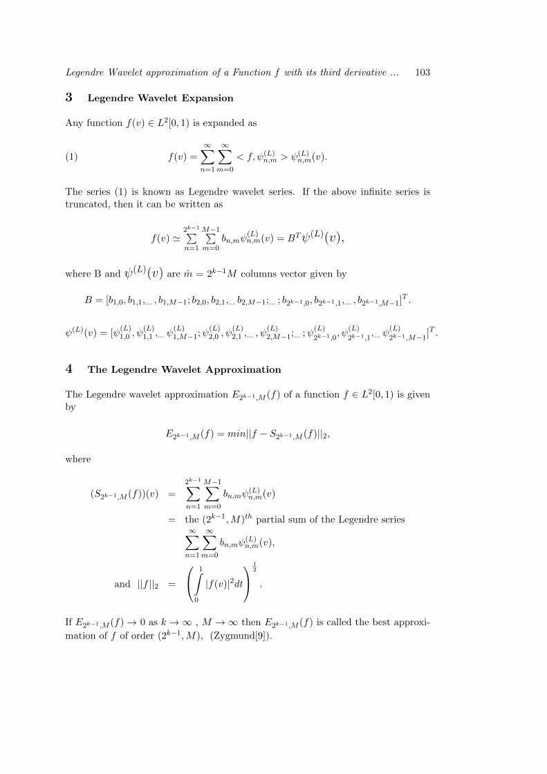
Legendre Wavelet approximation of a Function f with its third derivative ... 103
3 Legendre Wavelet Expansion
Any function f(v) ∈ L2[0, 1) is expanded as
(1) f(v) =∞∑n=1
∞∑m=0
< f,ψ(L)n,m > ψ(L)
n,m(v).
The series (1) is known as Legendre wavelet series. If the above infinite series istruncated, then it can be written as
f(v) '2k−1∑n=1
M−1∑m=0
bn,mψ(L)n,m(v) = BTψ(L)(v),
where B and ψ(L)(v) are m = 2k−1M columns vector given by
B = [b1,0, b1,1,... , b1,M−1; b2,0, b2,1,... b2,M−1;... ; b2k−1,0, b2k−1,1,... , b2k−1,M−1]T .
ψ(L)(v) = [ψ(L)1,0 , ψ
(L)1,1 ,... ψ
(L)1,M−1;ψ
(L)2,0 , ψ
(L)2,1 ,... , ψ
(L)2,M−1;... ;ψ
(L)
2k−1,0, ψ
(L)
2k−1,1,... ψ
(L)
2k−1,M−1]T .
4 The Legendre Wavelet Approximation
The Legendre wavelet approximation E2k−1,M (f) of a function f ∈ L2[0, 1) is givenby
E2k−1,M (f) = min||f − S2k−1,M (f)||2,
where
(S2k−1,M (f))(v) =
2k−1∑n=1
M−1∑m=0
bn,mψ(L)n,m(v)
= the (2k−1,M)th partial sum of the Legendre series∞∑n=1
∞∑m=0
bn,mψ(L)n,m(v),
and ||f ||2 =
1∫0
|f(v)|2dt
12
.
If E2k−1,M (f)→ 0 as k →∞ , M →∞ then E2k−1,M (f) is called the best approxi-
mation of f of order (2k−1,M), (Zygmund[9]).
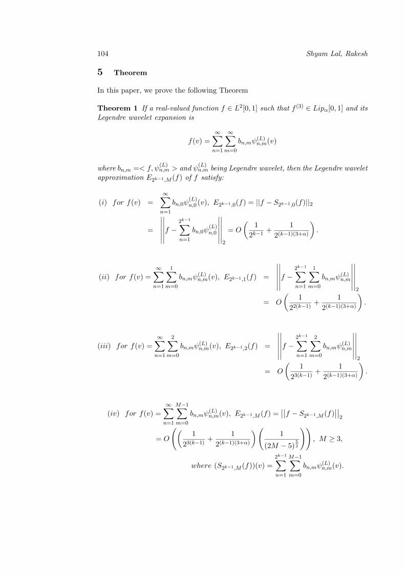
104 Shyam Lal, Rakesh
5 Theorem
In this paper, we prove the following Theorem
Theorem 1 If a real-valued function f ∈ L2[0, 1] such that f (3) ∈ Lipα[0, 1] and itsLegendre wavelet expansion is
f(v) =∞∑n=1
∞∑m=0
bn,mψ(L)n,m(v)
where bn,m =< f,ψ(L)n,m > and ψ
(L)n,m being Legendre wavelet, then the Legendre wavelet
approximation E2k−1,M (f) of f satisfy:
(i) for f(v) =∞∑n=1
bn,0ψ(L)n,0 (v), E2k−1,0(f) = ||f − S2k−1,0(f)||2
=
∣∣∣∣∣∣∣∣∣∣∣∣f −
2k−1∑n=1
bn,0ψ(L)n,0
∣∣∣∣∣∣∣∣∣∣∣∣2
= O
(1
2k−1+
1
2(k−1)(3+α)
).
(ii) for f(v) =∞∑n=1
1∑m=0
bn,mψ(L)n,m(v), E2k−1,1(f) =
∣∣∣∣∣∣∣∣∣∣∣∣f −
2k−1∑n=1
1∑m=0
bn,mψ(L)n,m
∣∣∣∣∣∣∣∣∣∣∣∣2
= O
(1
22(k−1)+
1
2(k−1)(3+α)
).
(iii) for f(v) =
∞∑n=1
2∑m=0
bn,mψ(L)n,m(v), E2k−1,2(f) =
∣∣∣∣∣∣∣∣∣∣∣∣f −
2k−1∑n=1
2∑m=0
bn,mψ(L)n,m
∣∣∣∣∣∣∣∣∣∣∣∣2
= O
(1
23(k−1)+
1
2(k−1)(3+α)
).
(iv) for f(v) =
∞∑n=1
M−1∑m=0
bn,mψ(L)n,m(v), E2k−1,M (f) =
∣∣∣∣f − S2k−1,M (f)∣∣∣∣2
= O
((1
23(k−1)+
1
2(k−1)(3+α)
)(1
(2M − 5)52
)), M ≥ 3,
where (S2k−1,M (f))(v) =2k−1∑n=1
M−1∑m=0
bn,mψ(L)n,m(v).
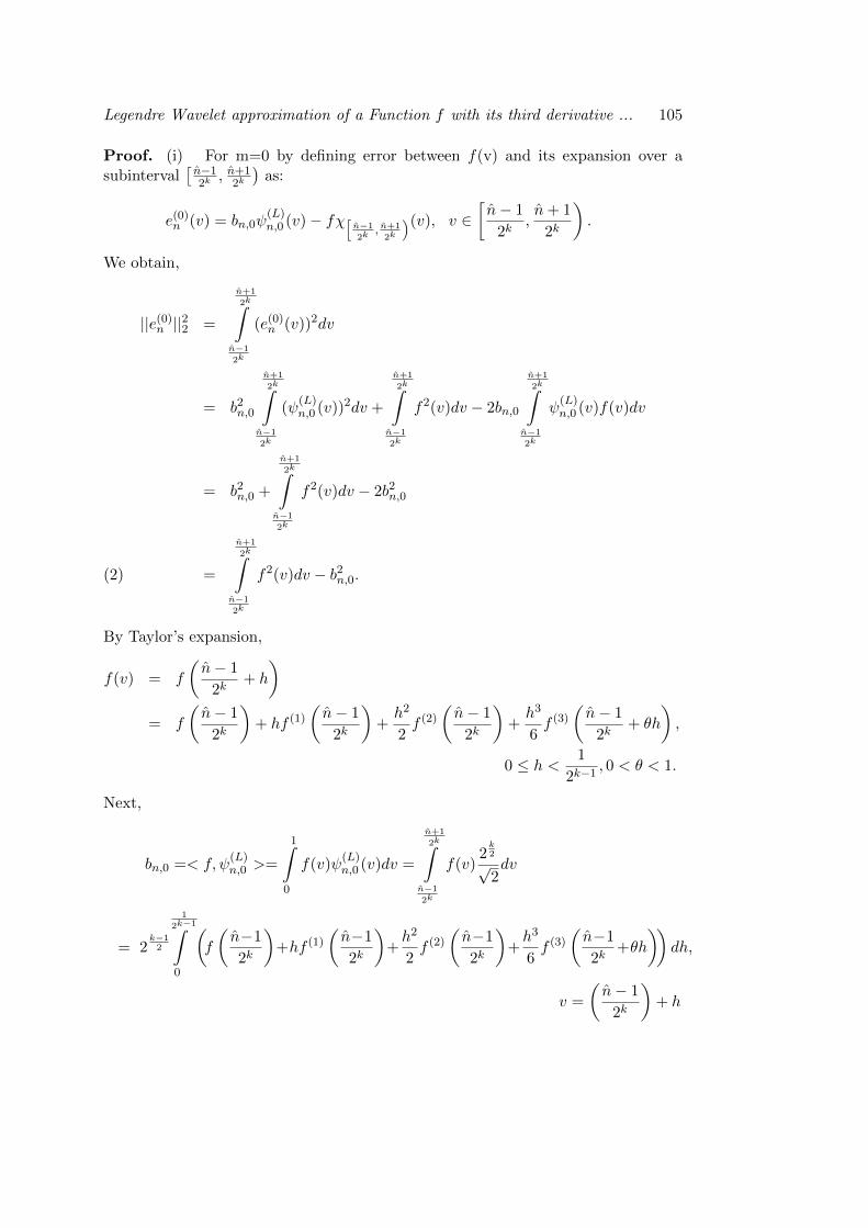
Legendre Wavelet approximation of a Function f with its third derivative ... 105
Proof. (i) For m=0 by defining error between f(v) and its expansion over asubinterval
[n−12k, n+1
2k
)as:
e(0)n (v) = bn,0ψ(L)n,0 (v)− fχ[ n−1
2k, n+1
2k
)(v), v ∈[n− 1
2k,n+ 1
2k
).
We obtain,
||e(0)n ||22 =
n+1
2k∫n−1
2k
(e(0)n (v))2dv
= b2n,0
n+1
2k∫n−1
2k
(ψ(L)n,0 (v))2dv +
n+1
2k∫n−1
2k
f2(v)dv − 2bn,0
n+1
2k∫n−1
2k
ψ(L)n,0 (v)f(v)dv
= b2n,0 +
n+1
2k∫n−1
2k
f2(v)dv − 2b2n,0
=
n+1
2k∫n−1
2k
f2(v)dv − b2n,0.(2)
By Taylor’s expansion,
f(v) = f
(n− 1
2k+ h
)= f
(n− 1
2k
)+ hf (1)
(n− 1
2k
)+h2
2f (2)
(n− 1
2k
)+h3
6f (3)
(n− 1
2k+ θh
),
0 ≤ h < 1
2k−1, 0 < θ < 1.
Next,
bn,0 =< f,ψ(L)n,0 >=
1∫0
f(v)ψ(L)n,0 (v)dv =
n+1
2k∫n−1
2k
f(v)2
k2
√2dv
= 2k−12
1
2k−1∫0
(f
(n−1
2k
)+hf (1)
(n−1
2k
)+h2
2f (2)
(n−1
2k
)+h3
6f (3)
(n−1
2k+θh
))dh,
v =
(n− 1
2k
)+ h
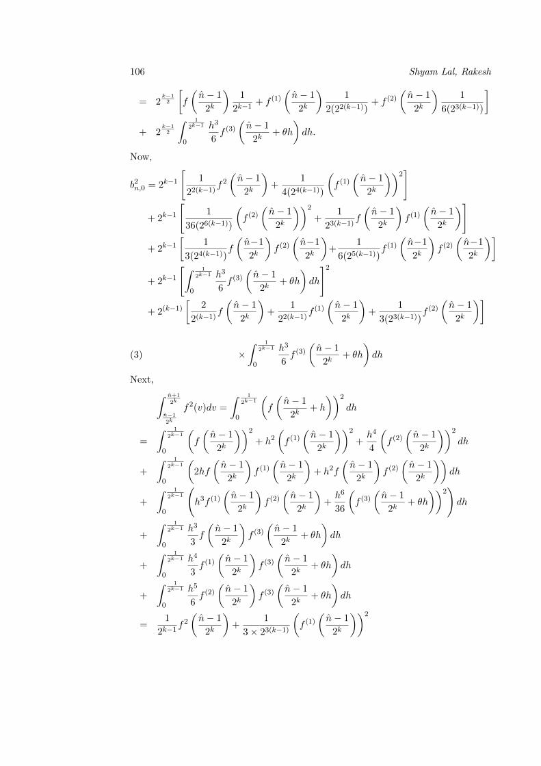
106 Shyam Lal, Rakesh
= 2k−12
[f
(n− 1
2k
)1
2k−1+ f (1)
(n− 1
2k
)1
2(22(k−1))+ f (2)
(n− 1
2k
)1
6(23(k−1))
]+ 2
k−12
∫ 1
2k−1
0
h3
6f (3)
(n− 1
2k+ θh
)dh.
Now,
b2n,0 = 2k−1
[1
22(k−1)f2(n− 1
2k
)+
1
4(24(k−1))
(f (1)
(n− 1
2k
))2]
+ 2k−1
[1
36(26(k−1))
(f (2)
(n− 1
2k
))2
+1
23(k−1)f
(n− 1
2k
)f (1)
(n− 1
2k
)]
+ 2k−1[
1
3(24(k−1))f
(n−1
2k
)f (2)
(n−1
2k
)+
1
6(25(k−1))f (1)
(n−1
2k
)f (2)
(n−1
2k
)]
+ 2k−1
[∫ 1
2k−1
0
h3
6f (3)
(n− 1
2k+ θh
)dh
]2+ 2(k−1)
[2
2(k−1)f
(n− 1
2k
)+
1
22(k−1)f (1)
(n− 1
2k
)+
1
3(23(k−1))f (2)
(n− 1
2k
)]
(3) ×∫ 1
2k−1
0
h3
6f (3)
(n− 1
2k+ θh
)dh
Next, ∫ n+1
2k
n−1
2k
f2(v)dv =
∫ 1
2k−1
0
(f
(n− 1
2k+ h
))2
dh
=
∫ 1
2k−1
0
(f
(n− 1
2k
))2
+ h2(f (1)
(n− 1
2k
))2
+h4
4
(f (2)
(n− 1
2k
))2
dh
+
∫ 1
2k−1
0
(2hf
(n− 1
2k
)f (1)
(n− 1
2k
)+ h2f
(n− 1
2k
)f (2)
(n− 1
2k
))dh
+
∫ 1
2k−1
0
(h3f (1)
(n− 1
2k
)f (2)
(n− 1
2k
)+h6
36
(f (3)
(n− 1
2k+ θh
))2)dh
+
∫ 1
2k−1
0
h3
3f
(n− 1
2k
)f (3)
(n− 1
2k+ θh
)dh
+
∫ 1
2k−1
0
h4
3f (1)
(n− 1
2k
)f (3)
(n− 1
2k+ θh
)dh
+
∫ 1
2k−1
0
h5
6f (2)
(n− 1
2k
)f (3)
(n− 1
2k+ θh
)dh
=1
2k−1f2(n− 1
2k
)+
1
3× 23(k−1)
(f (1)
(n− 1
2k
))2
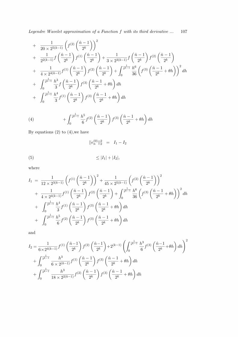
Legendre Wavelet approximation of a Function f with its third derivative ... 107
+1
20× 25(k−1)
(f (2)
(n− 1
2k
))2
+1
22(k−1)f
(n− 1
2k
)f (1)
(n− 1
2k
)+
1
3× 23(k−1)f
(n− 1
2k
)f (2)
(n− 1
2k
)+
1
4× 24(k−1)f (1)
(n− 1
2k
)f (2)
(n− 1
2k
)+
∫ 1
2k−1
0
h6
36
(f (3)
(n− 1
2k+ θh
))2
dh
+
∫ 1
2k−1
0
h3
3f
(n− 1
2k
)f (3)
(n− 1
2k+ θh
)dh
+
∫ 1
2k−1
0
h4
3f (1)
(n− 1
2k
)f (3)
(n− 1
2k+ θh
)dh
(4) +
∫ 1
2k−1
0
h5
6f (2)
(n− 1
2k
)f (3)
(n− 1
2k+ θh
)dh
By equations (2) to (4),we have
||e(0)n ||22 = I1 − I2
(5) ≤ |I1|+ |I2|,
where
I1 =1
12× 23(k−1)
(f (1)
(n− 1
2k
))2
+1
45× 25(k−1)
(f (2)
(n− 1
2k
))2
+1
4× 24(k−1)f (1)
(n− 1
2k
)f (2)
(n− 1
2k
)+
∫ 1
2k−1
0
h6
36
(f (3)
(n− 1
2k+ θh
))2
dh
+
∫ 1
2k−1
0
h4
3f (1)
(n− 1
2k
)f (3)
(n− 1
2k+ θh
)dh
+
∫ 1
2k−1
0
h5
6f (2)
(n− 1
2k
)f (3)
(n− 1
2k+ θh
)dh
and
I2 =1
6×24(k−1)f (1)
(n−1
2k
)f (2)
(n−1
2k
)+2(k−1)
(∫ 1
2k−1
0
h3
6f (3)
(n−1
2k+θh
)dh
)2
+
∫ 1
2k−1
0
h3
6× 2(k−1)f (1)
(n− 1
2k
)f (3)
(n− 1
2k+ θh
)dh
+
∫ 1
2k−1
0
h3
18× 22(k−1)f (2)
(n− 1
2k
)f (3)
(n− 1
2k+ θh
)dh
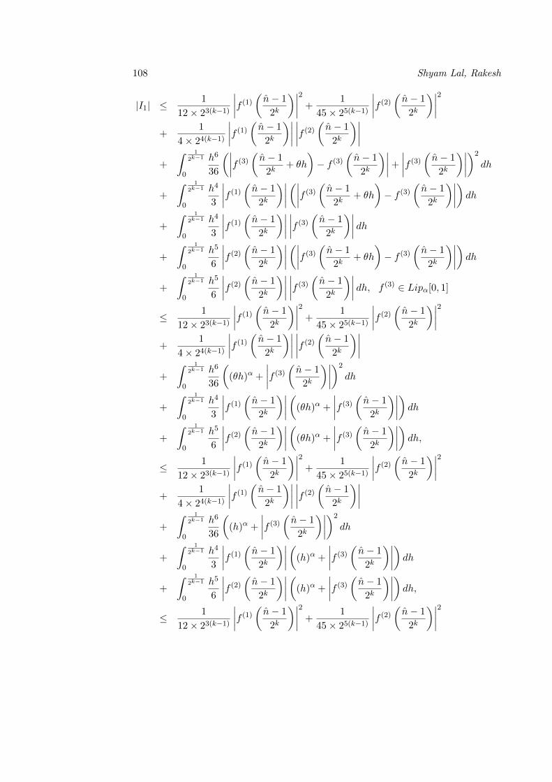
108 Shyam Lal, Rakesh
|I1| ≤1
12× 23(k−1)
∣∣∣∣f (1)( n− 1
2k
)∣∣∣∣2 +1
45× 25(k−1)
∣∣∣∣f (2)( n− 1
2k
)∣∣∣∣2+
1
4× 24(k−1)
∣∣∣∣f (1)( n− 1
2k
)∣∣∣∣ ∣∣∣∣f (2)( n− 1
2k
)∣∣∣∣+
∫ 1
2k−1
0
h6
36
(∣∣∣∣f (3)( n− 1
2k+ θh
)− f (3)
(n− 1
2k
)∣∣∣∣+
∣∣∣∣f (3)( n− 1
2k
)∣∣∣∣)2
dh
+
∫ 1
2k−1
0
h4
3
∣∣∣∣f (1)( n− 1
2k
)∣∣∣∣ (∣∣∣∣f (3)( n− 1
2k+ θh
)− f (3)
(n− 1
2k
)∣∣∣∣) dh+
∫ 1
2k−1
0
h4
3
∣∣∣∣f (1)( n− 1
2k
)∣∣∣∣ ∣∣∣∣f (3)( n− 1
2k
)∣∣∣∣ dh+
∫ 1
2k−1
0
h5
6
∣∣∣∣f (2)( n− 1
2k
)∣∣∣∣ (∣∣∣∣f (3)( n− 1
2k+ θh
)− f (3)
(n− 1
2k
)∣∣∣∣) dh+
∫ 1
2k−1
0
h5
6
∣∣∣∣f (2)( n− 1
2k
)∣∣∣∣ ∣∣∣∣f (3)( n− 1
2k
)∣∣∣∣ dh, f (3) ∈ Lipα[0, 1]
≤ 1
12× 23(k−1)
∣∣∣∣f (1)( n− 1
2k
)∣∣∣∣2 +1
45× 25(k−1)
∣∣∣∣f (2)( n− 1
2k
)∣∣∣∣2+
1
4× 24(k−1)
∣∣∣∣f (1)( n− 1
2k
)∣∣∣∣ ∣∣∣∣f (2)( n− 1
2k
)∣∣∣∣+
∫ 1
2k−1
0
h6
36
((θh)α +
∣∣∣∣f (3)( n− 1
2k
)∣∣∣∣)2
dh
+
∫ 1
2k−1
0
h4
3
∣∣∣∣f (1)( n− 1
2k
)∣∣∣∣ ((θh)α +
∣∣∣∣f (3)( n− 1
2k
)∣∣∣∣) dh+
∫ 1
2k−1
0
h5
6
∣∣∣∣f (2)( n− 1
2k
)∣∣∣∣ ((θh)α +
∣∣∣∣f (3)( n− 1
2k
)∣∣∣∣) dh,≤ 1
12× 23(k−1)
∣∣∣∣f (1)( n− 1
2k
)∣∣∣∣2 +1
45× 25(k−1)
∣∣∣∣f (2)( n− 1
2k
)∣∣∣∣2+
1
4× 24(k−1)
∣∣∣∣f (1)( n− 1
2k
)∣∣∣∣ ∣∣∣∣f (2)( n− 1
2k
)∣∣∣∣+
∫ 1
2k−1
0
h6
36
((h)α +
∣∣∣∣f (3)( n− 1
2k
)∣∣∣∣)2
dh
+
∫ 1
2k−1
0
h4
3
∣∣∣∣f (1)( n− 1
2k
)∣∣∣∣ ((h)α +
∣∣∣∣f (3)( n− 1
2k
)∣∣∣∣) dh+
∫ 1
2k−1
0
h5
6
∣∣∣∣f (2)( n− 1
2k
)∣∣∣∣ ((h)α +
∣∣∣∣f (3)( n− 1
2k
)∣∣∣∣) dh,≤ 1
12× 23(k−1)
∣∣∣∣f (1)( n− 1
2k
)∣∣∣∣2 +1
45× 25(k−1)
∣∣∣∣f (2)( n− 1
2k
)∣∣∣∣2
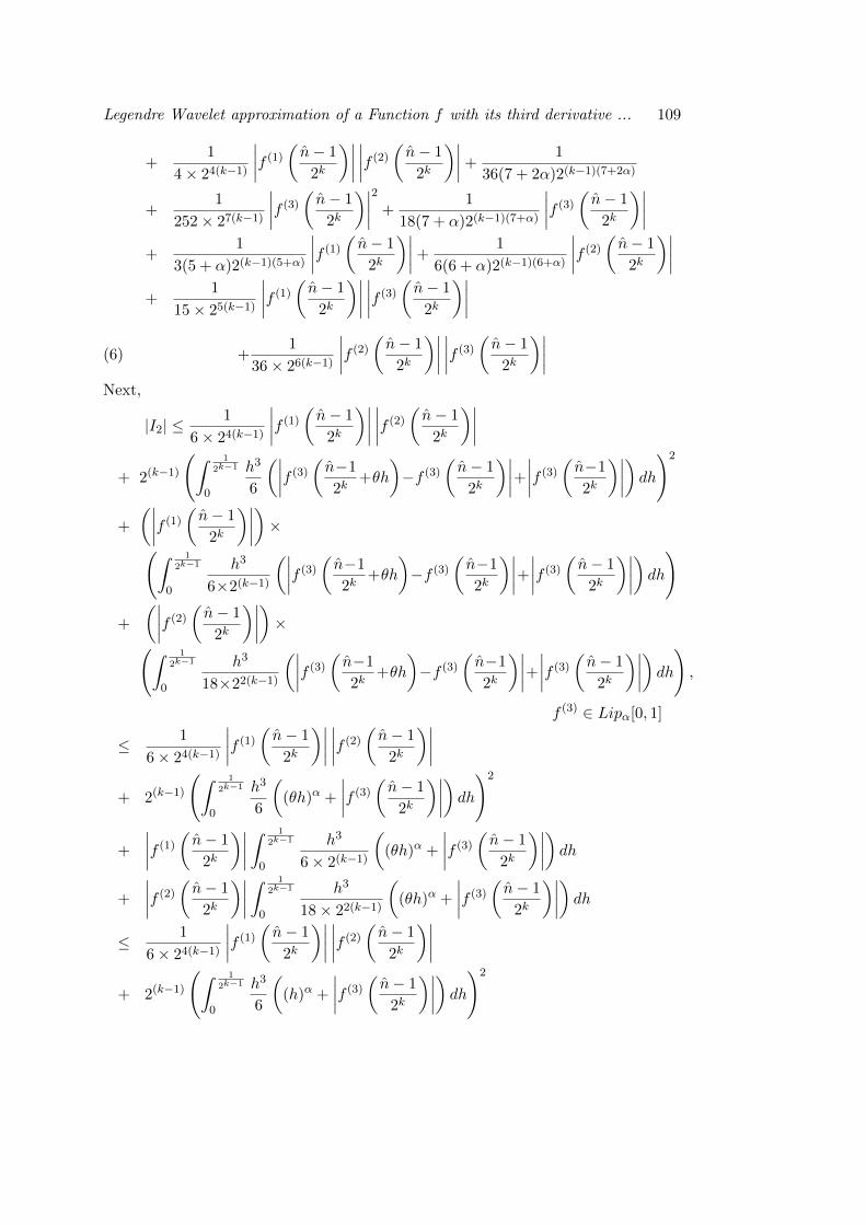
Legendre Wavelet approximation of a Function f with its third derivative ... 109
+1
4× 24(k−1)
∣∣∣∣f (1)( n− 1
2k
)∣∣∣∣ ∣∣∣∣f (2)( n− 1
2k
)∣∣∣∣+1
36(7 + 2α)2(k−1)(7+2α)
+1
252× 27(k−1)
∣∣∣∣f (3)( n− 1
2k
)∣∣∣∣2 +1
18(7 + α)2(k−1)(7+α)
∣∣∣∣f (3)( n− 1
2k
)∣∣∣∣+
1
3(5 + α)2(k−1)(5+α)
∣∣∣∣f (1)( n− 1
2k
)∣∣∣∣+1
6(6 + α)2(k−1)(6+α)
∣∣∣∣f (2)( n− 1
2k
)∣∣∣∣+
1
15× 25(k−1)
∣∣∣∣f (1)( n− 1
2k
)∣∣∣∣ ∣∣∣∣f (3)( n− 1
2k
)∣∣∣∣(6) +
1
36× 26(k−1)
∣∣∣∣f (2)( n− 1
2k
)∣∣∣∣ ∣∣∣∣f (3)( n− 1
2k
)∣∣∣∣Next,
|I2| ≤1
6× 24(k−1)
∣∣∣∣f (1)( n− 1
2k
)∣∣∣∣ ∣∣∣∣f (2)( n− 1
2k
)∣∣∣∣+ 2(k−1)
(∫ 1
2k−1
0
h3
6
(∣∣∣∣f (3)( n−1
2k+θh
)−f (3)
(n− 1
2k
)∣∣∣∣+∣∣∣∣f (3)( n−1
2k
)∣∣∣∣) dh)2
+
(∣∣∣∣f (1)( n− 1
2k
)∣∣∣∣)×(∫ 1
2k−1
0
h3
6×2(k−1)
(∣∣∣∣f (3)( n−1
2k+θh
)−f (3)
(n−1
2k
)∣∣∣∣+∣∣∣∣f (3)( n− 1
2k
)∣∣∣∣) dh)
+
(∣∣∣∣f (2)( n− 1
2k
)∣∣∣∣)×(∫ 1
2k−1
0
h3
18×22(k−1)
(∣∣∣∣f (3)( n−1
2k+θh
)−f (3)
(n−1
2k
)∣∣∣∣+∣∣∣∣f (3)( n− 1
2k
)∣∣∣∣) dh),
f (3) ∈ Lipα[0, 1]
≤ 1
6× 24(k−1)
∣∣∣∣f (1)( n− 1
2k
)∣∣∣∣ ∣∣∣∣f (2)( n− 1
2k
)∣∣∣∣+ 2(k−1)
(∫ 1
2k−1
0
h3
6
((θh)α +
∣∣∣∣f (3)( n− 1
2k
)∣∣∣∣) dh)2
+
∣∣∣∣f (1)( n− 1
2k
)∣∣∣∣ ∫ 1
2k−1
0
h3
6× 2(k−1)
((θh)α +
∣∣∣∣f (3)( n− 1
2k
)∣∣∣∣) dh+
∣∣∣∣f (2)( n− 1
2k
)∣∣∣∣ ∫ 1
2k−1
0
h3
18× 22(k−1)
((θh)α +
∣∣∣∣f (3)( n− 1
2k
)∣∣∣∣) dh≤ 1
6× 24(k−1)
∣∣∣∣f (1)( n− 1
2k
)∣∣∣∣ ∣∣∣∣f (2)( n− 1
2k
)∣∣∣∣+ 2(k−1)
(∫ 1
2k−1
0
h3
6
((h)α +
∣∣∣∣f (3)( n− 1
2k
)∣∣∣∣) dh)2
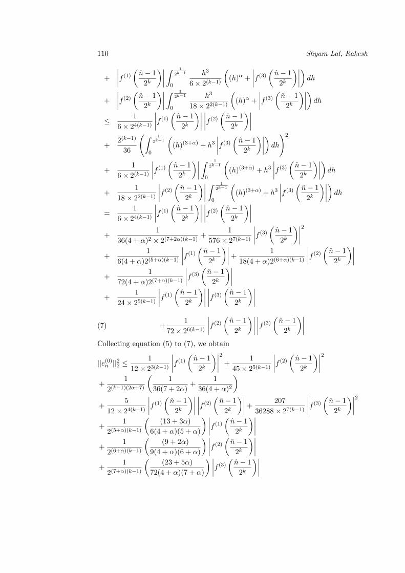
110 Shyam Lal, Rakesh
+
∣∣∣∣f (1)( n− 1
2k
)∣∣∣∣ ∫ 1
2k−1
0
h3
6× 2(k−1)
((h)α +
∣∣∣∣f (3)( n− 1
2k
)∣∣∣∣) dh+
∣∣∣∣f (2)( n− 1
2k
)∣∣∣∣ ∫ 1
2k−1
0
h3
18× 22(k−1)
((h)α +
∣∣∣∣f (3)( n− 1
2k
)∣∣∣∣) dh≤ 1
6× 24(k−1)
∣∣∣∣f (1)( n− 1
2k
)∣∣∣∣ ∣∣∣∣f (2)( n− 1
2k
)∣∣∣∣+
2(k−1)
36
(∫ 1
2k−1
0
((h)(3+α) + h3
∣∣∣∣f (3)( n− 1
2k
)∣∣∣∣) dh)2
+1
6× 2(k−1)
∣∣∣∣f (1)( n− 1
2k
)∣∣∣∣ ∫ 1
2k−1
0
((h)(3+α) + h3
∣∣∣∣f (3)( n− 1
2k
)∣∣∣∣) dh+
1
18× 22(k−1)
∣∣∣∣f (2)( n− 1
2k
)∣∣∣∣ ∫ 1
2k−1
0
((h)(3+α) + h3
∣∣∣∣f (3)( n− 1
2k
)∣∣∣∣) dh=
1
6× 24(k−1)
∣∣∣∣f (1)( n− 1
2k
)∣∣∣∣ ∣∣∣∣f (2)( n− 1
2k
)∣∣∣∣+
1
36(4 + α)2 × 2(7+2α)(k−1) +1
576× 27(k−1)
∣∣∣∣f (3)( n− 1
2k
)∣∣∣∣2+
1
6(4 + α)2(5+α)(k−1)
∣∣∣∣f (1)( n− 1
2k
)∣∣∣∣+1
18(4 + α)2(6+α)(k−1)
∣∣∣∣f (2)( n− 1
2k
)∣∣∣∣+
1
72(4 + α)2(7+α)(k−1)
∣∣∣∣f (3)( n− 1
2k
)∣∣∣∣+
1
24× 25(k−1)
∣∣∣∣f (1)( n− 1
2k
)∣∣∣∣ ∣∣∣∣f (3)( n− 1
2k
)∣∣∣∣(7) +
1
72× 26(k−1)
∣∣∣∣f (2)( n− 1
2k
)∣∣∣∣ ∣∣∣∣f (3)( n− 1
2k
)∣∣∣∣Collecting equation (5) to (7), we obtain
||e(0)n ||22 ≤1
12× 23(k−1)
∣∣∣∣f (1)( n− 1
2k
)∣∣∣∣2 +1
45× 25(k−1)
∣∣∣∣f (2)( n− 1
2k
)∣∣∣∣2+
1
2(k−1)(2α+7)
(1
36(7 + 2α)+
1
36(4 + α)2
)+
5
12× 24(k−1)
∣∣∣∣f (1)( n− 1
2k
)∣∣∣∣ ∣∣∣∣f (2)( n− 1
2k
)∣∣∣∣+207
36288× 27(k−1)
∣∣∣∣f (3)( n− 1
2k
)∣∣∣∣2+
1
2(5+α)(k−1)
((13 + 3α)
6(4 + α)(5 + α)
) ∣∣∣∣f (1)( n− 1
2k
)∣∣∣∣+
1
2(6+α)(k−1)
((9 + 2α)
9(4 + α)(6 + α)
) ∣∣∣∣f (2)( n− 1
2k
)∣∣∣∣+
1
2(7+α)(k−1)
((23 + 5α)
72(4 + α)(7 + α)
) ∣∣∣∣f (3)( n− 1
2k
)∣∣∣∣
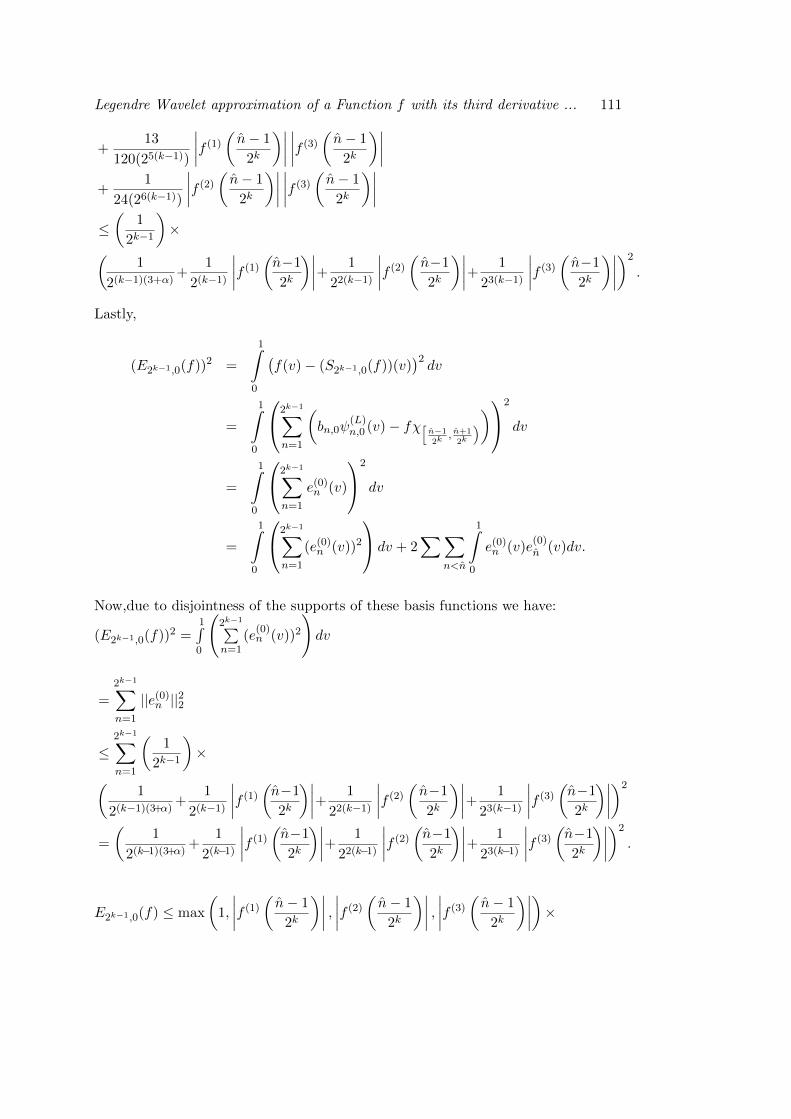
Legendre Wavelet approximation of a Function f with its third derivative ... 111
+13
120(25(k−1))
∣∣∣∣f (1)( n− 1
2k
)∣∣∣∣ ∣∣∣∣f (3)( n− 1
2k
)∣∣∣∣+
1
24(26(k−1))
∣∣∣∣f (2)( n− 1
2k
)∣∣∣∣ ∣∣∣∣f (3)( n− 1
2k
)∣∣∣∣≤(
1
2k−1
)×(
1
2(k−1)(3+α)+
1
2(k−1)
∣∣∣∣f (1)(n−1
2k
)∣∣∣∣+ 1
22(k−1)
∣∣∣∣f (2)( n−1
2k
)∣∣∣∣+ 1
23(k−1)
∣∣∣∣f (3)( n−1
2k
)∣∣∣∣)2
.
Lastly,
(E2k−1,0(f))2 =
1∫0
(f(v)− (S2k−1,0(f))(v)
)2dv
=
1∫0
2k−1∑n=1
(bn,0ψ
(L)n,0 (v)− fχ[ n−1
2k, n+1
2k
))2
dv
=
1∫0
2k−1∑n=1
e(0)n (v)
2
dv
=
1∫0
2k−1∑n=1
(e(0)n (v))2
dv + 2∑∑
n<n
1∫0
e(0)n (v)e(0)n (v)dv.
Now,due to disjointness of the supports of these basis functions we have:
(E2k−1,0(f))2 =1∫0
(2k−1∑n=1
(e(0)n (v))2
)dv
=2k−1∑n=1
||e(0)n ||22
≤2k−1∑n=1
(1
2k−1
)×
(1
2(k−1)(3+α)+
1
2(k−1)
∣∣∣∣f (1)(n−1
2k
)∣∣∣∣+ 1
22(k−1)
∣∣∣∣f (2)( n−1
2k
)∣∣∣∣+ 1
23(k−1)
∣∣∣∣f (3)(n−1
2k
)∣∣∣∣)2
=
(1
2(k−1)(3+α)+
1
2(k−1)
∣∣∣∣f (1)(n−1
2k
)∣∣∣∣+ 1
22(k−1)
∣∣∣∣f (2)(n−1
2k
)∣∣∣∣+ 1
23(k−1)
∣∣∣∣f (3)(n−1
2k
)∣∣∣∣)2
.
E2k−1,0(f) ≤ max
(1,
∣∣∣∣f (1)( n− 1
2k
)∣∣∣∣ , ∣∣∣∣f (2)( n− 1
2k
)∣∣∣∣ , ∣∣∣∣f (3)( n− 1
2k
)∣∣∣∣)×
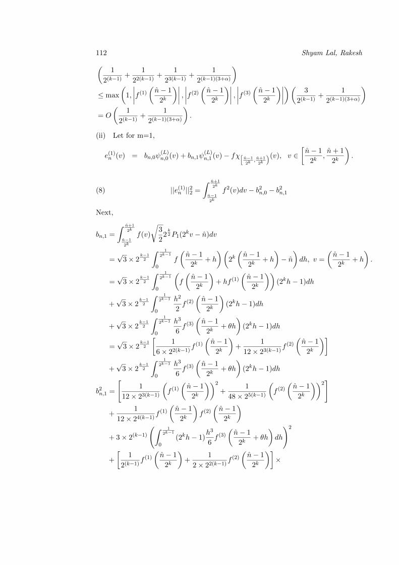
112 Shyam Lal, Rakesh(1
2(k−1)+
1
22(k−1)+
1
23(k−1)+
1
2(k−1)(3+α)
)≤ max
(1,
∣∣∣∣f (1)( n− 1
2k
)∣∣∣∣ , ∣∣∣∣f (2)( n− 1
2k
)∣∣∣∣ , ∣∣∣∣f (3)( n− 1
2k
)∣∣∣∣)( 3
2(k−1)+
1
2(k−1)(3+α)
)= O
(1
2(k−1)+
1
2(k−1)(3+α)
).
(ii) Let for m=1,
e(1)n (v) = bn,0ψ(L)n,0 (v) + bn,1ψ
(L)n,1 (v)− fχ[ n−1
2k, n+1
2k
)(v), v ∈[n− 1
2k,n+ 1
2k
).
(8) ||e(1)n ||22 =
∫ n+1
2k
n−1
2k
f2(v)dv − b2n,0 − b2n,1
Next,
bn,1 =
∫ n+1
2k
n−1
2k
f(v)
√3
22
k2P1(2
kv − n)dv
=√
3× 2k−12
∫ 1
2k−1
0f
(n− 1
2k+ h
)(2k(n− 1
2k+ h
)− n
)dh, v =
(n− 1
2k+ h
).
=√
3× 2k−12
∫ 1
2k−1
0
(f
(n− 1
2k
)+ hf (1)
(n− 1
2k
))(2kh− 1)dh
+√
3× 2k−12
∫ 1
2k−1
0
h2
2f (2)
(n− 1
2k
)(2kh− 1)dh
+√
3× 2k−12
∫ 1
2k−1
0
h3
6f (3)
(n− 1
2k+ θh
)(2kh− 1)dh
=√
3× 2k−12
[1
6× 22(k−1)f (1)
(n− 1
2k
)+
1
12× 23(k−1)f (2)
(n− 1
2k
)]+√
3× 2k−12
∫ 1
2k−1
0
h3
6f (3)
(n− 1
2k+ θh
)(2kh− 1)dh
b2n,1 =
[1
12× 23(k−1)
(f (1)
(n− 1
2k
))2
+1
48× 25(k−1)
(f (2)
(n− 1
2k
))2]
+1
12× 24(k−1)f (1)
(n− 1
2k
)f (2)
(n− 1
2k
)+ 3× 2(k−1)
(∫ 1
2k−1
0(2kh− 1)
h3
6f (3)
(n− 1
2k+ θh
)dh
)2
+
[1
2(k−1)f (1)
(n− 1
2k
)+
1
2× 22(k−1)f (2)
(n− 1
2k
)]×
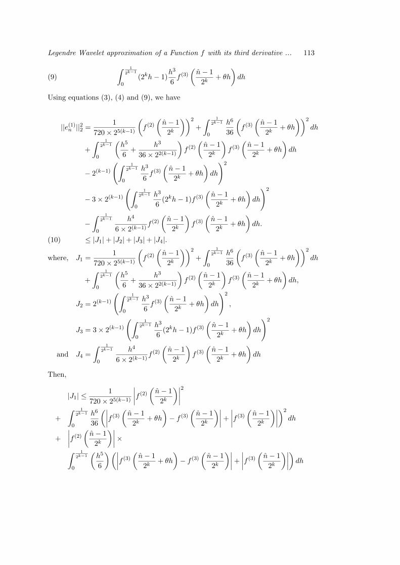
Legendre Wavelet approximation of a Function f with its third derivative ... 113
(9)
∫ 1
2k−1
0(2kh− 1)
h3
6f (3)
(n− 1
2k+ θh
)dh
Using equations (3), (4) and (9), we have
||e(1)n ||22 =1
720× 25(k−1)
(f (2)
(n− 1
2k
))2
+
∫ 1
2k−1
0
h6
36
(f (3)
(n− 1
2k+ θh
))2
dh
+
∫ 1
2k−1
0
(h5
6+
h3
36× 22(k−1)
)f (2)
(n− 1
2k
)f (3)
(n− 1
2k+ θh
)dh
− 2(k−1)
(∫ 1
2k−1
0
h3
6f (3)
(n− 1
2k+ θh
)dh
)2
− 3× 2(k−1)
(∫ 1
2k−1
0
h3
6(2kh− 1)f (3)
(n− 1
2k+ θh
)dh
)2
−∫ 1
2k−1
0
h4
6× 2(k−1)f (2)
(n− 1
2k
)f (3)
(n− 1
2k+ θh
)dh.
≤ |J1|+ |J2|+ |J3|+ |J4|.(10)
where, J1 =1
720× 25(k−1)
(f (2)
(n− 1
2k
))2
+
∫ 1
2k−1
0
h6
36
(f (3)
(n− 1
2k+ θh
))2
dh
+
∫ 1
2k−1
0
(h5
6+
h3
36× 22(k−1)
)f (2)
(n− 1
2k
)f (3)
(n− 1
2k+ θh
)dh,
J2 = 2(k−1)
(∫ 1
2k−1
0
h3
6f (3)
(n− 1
2k+ θh
)dh
)2
,
J3 = 3× 2(k−1)
(∫ 1
2k−1
0
h3
6(2kh− 1)f (3)
(n− 1
2k+ θh
)dh
)2
and J4 =
∫ 1
2k−1
0
h4
6× 2(k−1)f (2)
(n− 1
2k
)f (3)
(n− 1
2k+ θh
)dh
Then,
|J1| ≤1
720× 25(k−1)
∣∣∣∣f (2)( n− 1
2k
)∣∣∣∣2+
∫ 1
2k−1
0
h6
36
(∣∣∣∣f (3)( n− 1
2k+ θh
)− f (3)
(n− 1
2k
)∣∣∣∣+
∣∣∣∣f (3)( n− 1
2k
)∣∣∣∣)2
dh
+
∣∣∣∣f (2)( n− 1
2k
)∣∣∣∣×∫ 1
2k−1
0
(h5
6
)(∣∣∣∣f (3)( n− 1
2k+ θh
)− f (3)
(n− 1
2k
)∣∣∣∣+
∣∣∣∣f (3)( n− 1
2k
)∣∣∣∣) dh
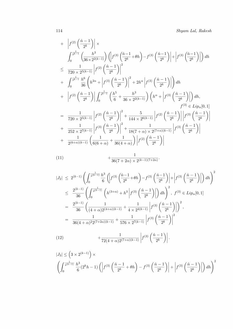
114 Shyam Lal, Rakesh
+
∣∣∣∣f (2)( n− 1
2k
)∣∣∣∣×∫ 1
2k−1
0
(h3
36×22(k−1)
)(∣∣∣∣f (3)(n−1
2k+θh
)−f (3)
(n−1
2k
)∣∣∣∣+∣∣∣∣f (3)(n−1
2k
)∣∣∣∣) dh≤ 1
720× 25(k−1)
∣∣∣∣f (2)( n− 1
2k
)∣∣∣∣2+
∫ 1
2k−1
0
h6
36
(h2α +
∣∣∣∣f (3)( n− 1
2k
)∣∣∣∣2 + 2hα∣∣∣∣f (3)( n− 1
2k
)∣∣∣∣)dh
+
∣∣∣∣f (2)( n− 1
2k
)∣∣∣∣ ∫ 1
2k−1
0
(h5
6+
h3
36× 22(k−1)
)(hα +
∣∣∣∣f (3)( n− 1
2k
)∣∣∣∣) dh,f (3) ∈ Lipα[0, 1]
=1
720× 25(k−1)
∣∣∣∣f (2)( n− 1
2k
)∣∣∣∣2 +5
144× 26(k−1)
∣∣∣∣f (2)( n− 1
2k
)∣∣∣∣ ∣∣∣∣f (3)( n− 1
2k
)∣∣∣∣+
1
252× 27(k−1)
∣∣∣∣f (3)( n− 1
2k
)∣∣∣∣2 +1
18(7 + α)× 2(7+α)(k−1)
∣∣∣∣f (3)( n− 1
2k
)∣∣∣∣+
1
2(6+α)(k−1)
(1
6(6 + α)+
1
36(4 + α)
) ∣∣∣∣f (2)( n− 1
2k
)∣∣∣∣(11) +
1
36(7 + 2α)× 2(k−1)(7+2α).
|J2| ≤ 2(k−1)
(∫ 1
2(k−1)
0
h3
6
(∣∣∣∣f (3)(n−1
2k+θh
)−f (3)
(n−1
2k
)∣∣∣∣+∣∣∣∣f (3)( n− 1
2k
)∣∣∣∣) dh)2
≤ 2(k−1)
36
(∫ 1
2(k−1)
0
(h(3+α) + h3
∣∣∣∣f (3)( n− 1
2k
)∣∣∣∣) dh)2
, f (3) ∈ Lipα[0, 1]
=2(k−1)
36
(1
(4 + α)2(4+α)(k−1)+
1
4× 24(k−1)
∣∣∣∣f (3)( n− 1
2k
)∣∣∣∣)2
,
=1
36(4 + α)22(7+2α)(k−1) +1
576× 27(k−1)
∣∣∣∣f (3)( n− 1
2k
)∣∣∣∣2
(12) +1
72(4 + α)2(7+α)(k−1)
∣∣∣∣f (3)( n− 1
2k
)∣∣∣∣ .|J3| ≤
(3× 2(k−1)
)×(∫ 1
2(k−1)
0
h3
6(2kh− 1)
(∣∣∣∣f (3)( n− 1
2k+ θh
)− f (3)
(n− 1
2k
)∣∣∣∣+
∣∣∣∣f (3)( n− 1
2k
)∣∣∣∣) dh)2
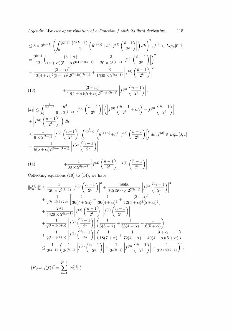
Legendre Wavelet approximation of a Function f with its third derivative ... 115
≤ 3× 2(k−1)
(∫ 1
2(k−1)
0
(2kh−1)
6
(h(3+α)+h3
∣∣∣∣f (3)( n−1
2k
)∣∣∣∣) dh)2
, f (3) ∈ Lipα[0, 1]
=2k−1
12
((3 + α)
(4 + α)(5 + α)2(4+α)(k−1)+
3
20× 24(k−1)
∣∣∣∣f (3)( n− 1
2k
)∣∣∣∣)2
=(3 + α)2
12(4 + α)2(5 + α)22(7+2α)(k−1) +3
1600× 27(k−1)
∣∣∣∣f (3)( n− 1
2k
)∣∣∣∣2
(13) +(3 + α)
40(4 + α)(5 + α)2(7+α)(k−1)
∣∣∣∣f (3)( n− 1
2k
)∣∣∣∣ .|J4| ≤
∫ 1
2(k−1)
0
h4
6× 2(k−1)
∣∣∣∣f (2)( n− 1
2k
)∣∣∣∣ (∣∣∣∣f (3)( n− 1
2k+ θh
)− f (3)
(n− 1
2k
)∣∣∣∣+
∣∣∣∣f (3)( n− 1
2k
)∣∣∣∣) dh≤ 1
6× 2(k−1)
∣∣∣∣f (2)( n−1
2k
)∣∣∣∣ ∫ 1
2(k−1)
0
(h(4+α)+h4
∣∣∣∣f (3)( n− 1
2k
)∣∣∣∣) dh, f (3) ∈ Lipα[0, 1]
=1
6(5 + α)2(6+α)(k−1)
∣∣∣∣f (2)( n− 1
2k
)∣∣∣∣(14) +
1
30× 26(k−1)
∣∣∣∣f (2)( n− 1
2k
)∣∣∣∣ ∣∣∣∣f (3)( n− 1
2k
)∣∣∣∣Collecting equations (10) to (14), we have
||e(1)n ||22 ≤1
720× 25(k−1)
∣∣∣∣f (2)( n− 1
2k
)∣∣∣∣2 +48896
6451200× 27(k−1)
∣∣∣∣f (3)( n− 1
2k
)∣∣∣∣2+
1
2(k−1)(7+2α)
[1
36(7 + 2α)+
1
36(4 + α)2+
(3 + α)2
12(4 + α)2(5 + α)2
]+
294
4320× 26(k−1)
∣∣∣∣f (2)( n− 1
2k
)∣∣∣∣ ∣∣∣∣f (3)( n− 1
2k
)∣∣∣∣+
1
2(k−1)(6+α)
∣∣∣∣f (2)( n− 1
2k
)∣∣∣∣ ( 1
6(6 + α)+
1
36(4 + α)+
1
6(5 + α)
)+
1
2(k−1)(7+α)
∣∣∣∣f (3)( n− 1
2k
)∣∣∣∣ ( 1
18(7 + α)+
1
72(4 + α)+
3 + α
40(4 + α)(5 + α)
)≤ 1
2(k−1)
(1
22(k−1)
∣∣∣∣f (2)( n− 1
2k
)∣∣∣∣+1
23(k−1)
∣∣∣∣f (3)( n− 1
2k
)∣∣∣∣+1
2(3+α)(k−1)
)2
.
(E2k−1,1(f))2 =2k−1∑n=1
||e(1)n ||22
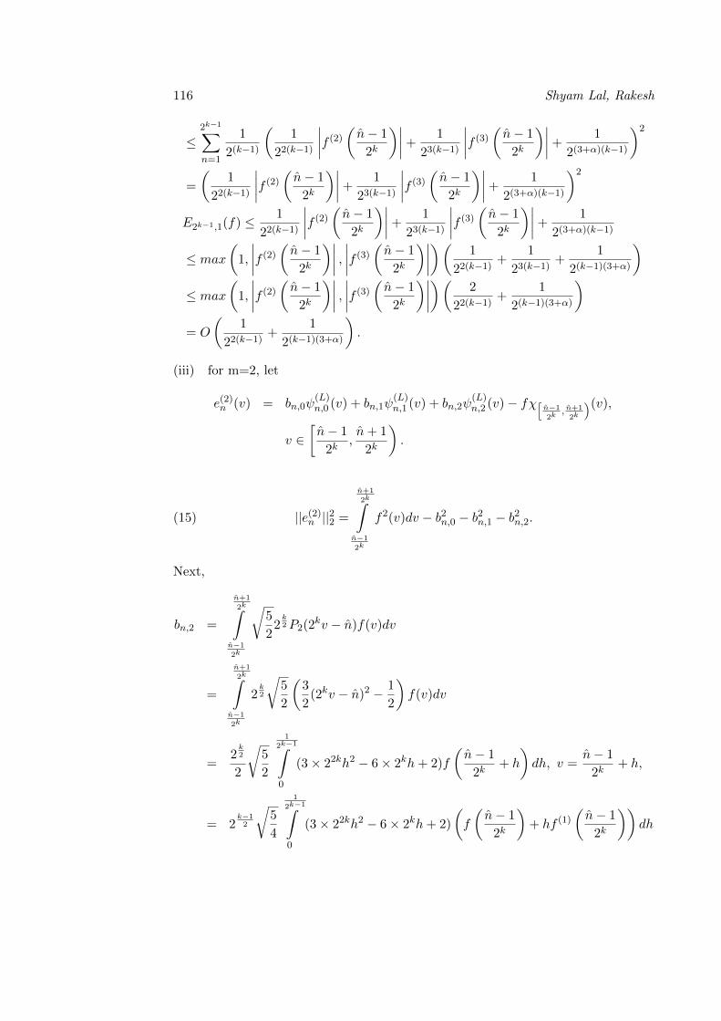
116 Shyam Lal, Rakesh
≤2k−1∑n=1
1
2(k−1)
(1
22(k−1)
∣∣∣∣f (2)( n− 1
2k
)∣∣∣∣+1
23(k−1)
∣∣∣∣f (3)( n− 1
2k
)∣∣∣∣+1
2(3+α)(k−1)
)2
=
(1
22(k−1)
∣∣∣∣f (2)( n− 1
2k
)∣∣∣∣+1
23(k−1)
∣∣∣∣f (3)( n− 1
2k
)∣∣∣∣+1
2(3+α)(k−1)
)2
E2k−1,1(f) ≤ 1
22(k−1)
∣∣∣∣f (2)( n− 1
2k
)∣∣∣∣+1
23(k−1)
∣∣∣∣f (3)( n− 1
2k
)∣∣∣∣+1
2(3+α)(k−1)
≤ max(
1,
∣∣∣∣f (2)( n− 1
2k
)∣∣∣∣ , ∣∣∣∣f (3)( n− 1
2k
)∣∣∣∣)( 1
22(k−1)+
1
23(k−1)+
1
2(k−1)(3+α)
)≤ max
(1,
∣∣∣∣f (2)( n− 1
2k
)∣∣∣∣ , ∣∣∣∣f (3)( n− 1
2k
)∣∣∣∣)( 2
22(k−1)+
1
2(k−1)(3+α)
)= O
(1
22(k−1)+
1
2(k−1)(3+α)
).
(iii) for m=2, let
e(2)n (v) = bn,0ψ(L)n,0 (v) + bn,1ψ
(L)n,1 (v) + bn,2ψ
(L)n,2 (v)− fχ[ n−1
2k, n+1
2k
)(v),
v ∈[n− 1
2k,n+ 1
2k
).
(15) ||e(2)n ||22 =
n+1
2k∫n−1
2k
f2(v)dv − b2n,0 − b2n,1 − b2n,2.
Next,
bn,2 =
n+1
2k∫n−1
2k
√5
22
k2P2(2
kv − n)f(v)dv
=
n+1
2k∫n−1
2k
2k2
√5
2
(3
2(2kv − n)2 − 1
2
)f(v)dv
=2
k2
2
√5
2
1
2k−1∫0
(3× 22kh2 − 6× 2kh+ 2)f
(n− 1
2k+ h
)dh, v =
n− 1
2k+ h,
= 2k−12
√5
4
1
2k−1∫0
(3× 22kh2 − 6× 2kh+ 2)
(f
(n− 1
2k
)+ hf (1)
(n− 1
2k
))dh
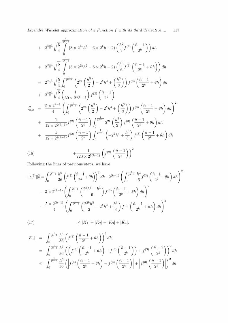
Legendre Wavelet approximation of a Function f with its third derivative ... 117
+ 2k−12
√5
4
1
2k−1∫0
(3× 22kh2 − 6× 2kh+ 2)
(h2
2f (2)
(n− 1
2k
))dh
+ 2k−12
√5
4
1
2k−1∫0
(3× 22kh2 − 6× 2kh+ 2)
(h3
6f (3)
(n− 1
2k+ θh
))dh
= 2k−12
√5
4
∫ 1
2k−1
0
(22k(h5
2
)− 2kh4 +
(h3
3
))f (3)
(n− 1
2k+ θh
)dh
+ 2k−12
√5
4
(1
30× 23(k−1)
)f (2)
(n− 1
2k
)b2n,2 =
5× 2k−1
4
(∫ 1
2k−1
0
(22k(h5
2
)− 2kh4 +
(h3
3
))f (3)
(n− 1
2k+ θh
)dh
)2
+1
12× 22(k−1)f (2)
(n− 1
2k
)∫ 1
2k−1
022k(h5
2
)f (3)
(n− 1
2k+ θh
)dh
+1
12× 22(k−1)f (2)
(n− 1
2k
)∫ 1
2k−1
0
(−2kh4 +
h3
3
)f (3)
(n− 1
2k+ θh
)dh
(16) +1
720× 25(k−1)
(f (2)
(n− 1
2k
))2
Following the lines of previous steps, we have
||e(2)n ||22 =
∫ 1
2k−1
0
h6
36
(f (3)
(n−1
2k+θh
))2
dh−2(k−1)
(∫ 1
2k−1
0
h3
6f (3)
(n−1
2k+θh
)dh
)2
− 3× 2(k−1)
(∫ 1
2k−1
0
(2kh4 − h3
6
)f (3)
(n− 1
2k+ θh
)dh
)2
− 5× 2(k−1)
4
(∫ 1
2k−1
0
(22kh5
2− 2kh4 +
h3
3
)f (3)
(n− 1
2k+ θh
)dh
)2
(17) ≤ |K1|+ |K2|+ |K3|+ |K4|.
|K1| =
∫ 1
2k−1
0
h6
36
(f (3)
(n− 1
2k+ θh
))2
dh
=
∫ 1
2k−1
0
h6
36
((f (3)
(n− 1
2k+ θh
)− f (3)
(n− 1
2k
))+ f (3)
(n− 1
2k
))2
dh
≤∫ 1
2k−1
0
h6
36
(∣∣∣∣f (3)( n− 1
2k+ θh
)− f (3)
(n− 1
2k
)∣∣∣∣+
∣∣∣∣f (3)( n− 1
2k
)∣∣∣∣)2
dh
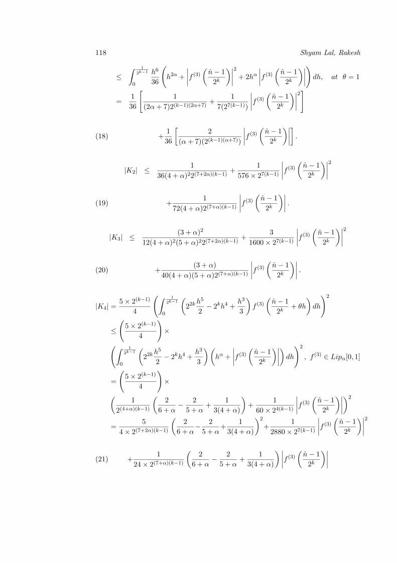
118 Shyam Lal, Rakesh
≤∫ 1
2k−1
0
h6
36
(h2α +
∣∣∣∣f (3)( n− 1
2k
)∣∣∣∣2 + 2hα∣∣∣∣f (3)( n− 1
2k
)∣∣∣∣)dh, at θ = 1
=1
36
[1
(2α+ 7)2(k−1)(2α+7)+
1
7(27(k−1))
∣∣∣∣f (3)( n− 1
2k
)∣∣∣∣2]
(18) +1
36
[2
(α+ 7)(2(k−1)(α+7))
∣∣∣∣f (3)( n− 1
2k
)∣∣∣∣] .
|K2| ≤1
36(4 + α)22(7+2α)(k−1) +1
576× 27(k−1)
∣∣∣∣f (3)( n− 1
2k
)∣∣∣∣2
(19) +1
72(4 + α)2(7+α)(k−1)
∣∣∣∣f (3)( n− 1
2k
)∣∣∣∣ .
|K3| ≤(3 + α)2
12(4 + α)2(5 + α)22(7+2α)(k−1) +3
1600× 27(k−1)
∣∣∣∣f (3)( n− 1
2k
)∣∣∣∣2
(20) +(3 + α)
40(4 + α)(5 + α)2(7+α)(k−1)
∣∣∣∣f (3)( n− 1
2k
)∣∣∣∣ .
|K4| =5× 2(k−1)
4
(∫ 1
2k−1
0
(22k
h5
2− 2kh4 +
h3
3
)f (3)
(n− 1
2k+ θh
)dh
)2
≤
(5× 2(k−1)
4
)×(∫ 1
2k−1
0
(22k
h5
2− 2kh4 +
h3
3
)(hα +
∣∣∣∣f (3)( n− 1
2k
)∣∣∣∣) dh)2
, f (3) ∈ Lipα[0, 1]
=
(5× 2(k−1)
4
)×(
1
2(4+α)(k−1)
(2
6 + α− 2
5 + α+
1
3(4 + α)
)+
1
60× 24(k−1)
∣∣∣∣f (3)( n− 1
2k
)∣∣∣∣)2
=5
4× 2(7+2α)(k−1)
(2
6 + α− 2
5 + α+
1
3(4 + α)
)2
+1
2880× 27(k−1)
∣∣∣∣f (3)( n− 1
2k
)∣∣∣∣2
(21) +1
24× 2(7+α)(k−1)
(2
6 + α− 2
5 + α+
1
3(4 + α)
) ∣∣∣∣f (3)( n− 1
2k
)∣∣∣∣
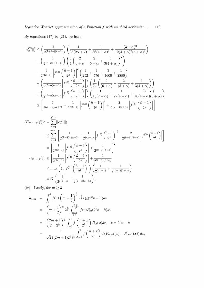
Legendre Wavelet approximation of a Function f with its third derivative ... 119
By equations (17) to (21), we have
||e(2)n ||22 ≤(
1
2(7+2α)(k−1)
)(1
36(2α+ 7)+
1
36(4 + α)2+
(3 + α)2
12(4 + α)2(5 + α)2
)+
(1
2(7+2α)(k−1)
)(5
4
(2
6 + α− 2
5 + α+
1
3(4 + α)
)2)
+1
27(k−1)
∣∣∣∣f (3)( n− 1
2k
)∣∣∣∣2( 1
252+
1
576+
3
1600+
1
2880
)+
(1
2(7+α)(k−1)
∣∣∣∣f (3)( n− 1
2k
)∣∣∣∣)( 1
24
(2
(6 + α)− 2
(5 + α)+
1
3(4 + α)
))+
(1
2(7+α)(k−1)
∣∣∣∣f (3)( n− 1
2k
)∣∣∣∣)( 1
18(7 + α)+
1
72(4 + α)+
(3 + α)
40(4 + α)(5 + α)
)≤
[1
2(k−1)(2α+7)+
1
27(k−1)
∣∣∣∣f (3)( n− 1
2k
)∣∣∣∣2 +2
2(k−1)(7+α)
∣∣∣∣f (3)( n− 1
2k
)∣∣∣∣]
(E2k−1,2(f))2 =2k−1∑n=1
||e(2)n ||22
≤2k−1∑n=1
[1
2(k−1)(2α+7)+
1
27(k−1)
∣∣∣∣f (3)(n−1
2k
)∣∣∣∣2+2
2(k−1)(7+α)
∣∣∣∣f (3)(n−1
2k
)∣∣∣∣]
=
[1
23(k−1)
∣∣∣∣f (3)( n− 1
2k
)∣∣∣∣+1
2(k−1)(3+α)
]2E2k−1,2(f) ≤
[1
23(k−1)
∣∣∣∣f (3)( n− 1
2k
)∣∣∣∣+1
2(k−1)(3+α)
]≤ max
(1,
∣∣∣∣f (3)( n− 1
2k
)∣∣∣∣)( 1
23(k−1)+
1
2(k−1)(3+α)
)= O
(1
23(k−1)+
1
2(k−1)(3+α)
).
(iv) Lastly, for m ≥ 3
bn,m =
∫ 1
0f(v)
(m+
1
2
) 12
2k2Pm(2kv − n)dv
=
(m+
1
2
) 12
2k2
∫ n+1
2k
n−1
2k
f(v)Pm(2kv − n)dv
=
(2m+ 1
2× 2k
) 12∫ 1
−1f
(n+ x
2k
)Pm(x)dx, x = 2kv − n
=1
√2 ((2m+ 1)2k)
12
∫ 1
−1f
(n+ x
2k
)d (Pm+1(x)− Pm−1(x)) dx,
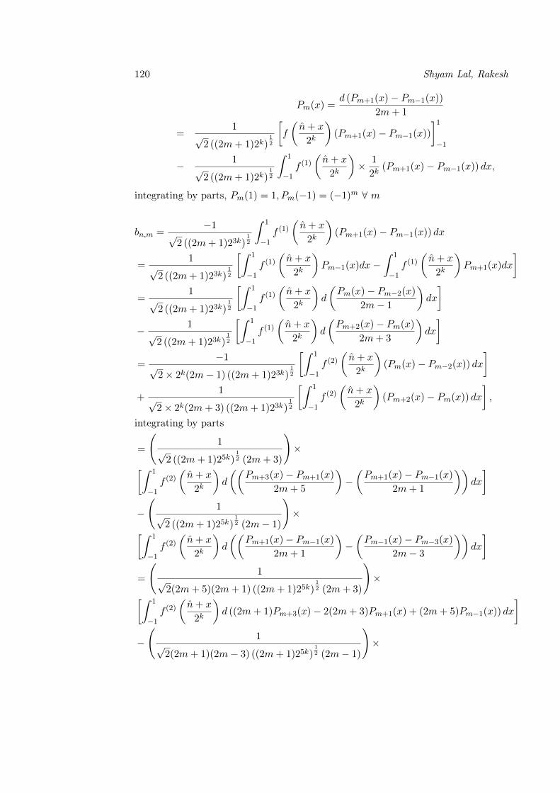
120 Shyam Lal, Rakesh
Pm(x) =d (Pm+1(x)− Pm−1(x))
2m+ 1
=1
√2 ((2m+ 1)2k)
12
[f
(n+ x
2k
)(Pm+1(x)− Pm−1(x))
]1−1
− 1√
2 ((2m+ 1)2k)12
∫ 1
−1f (1)
(n+ x
2k
)× 1
2k(Pm+1(x)− Pm−1(x)) dx,
integrating by parts, Pm(1) = 1, Pm(−1) = (−1)m ∀ m
bn,m =−1
√2 ((2m+ 1)23k)
12
∫ 1
−1f (1)
(n+ x
2k
)(Pm+1(x)− Pm−1(x)) dx
=1
√2 ((2m+ 1)23k)
12
[∫ 1
−1f (1)
(n+ x
2k
)Pm−1(x)dx−
∫ 1
−1f (1)
(n+ x
2k
)Pm+1(x)dx
]=
1√
2 ((2m+ 1)23k)12
[∫ 1
−1f (1)
(n+ x
2k
)d
(Pm(x)− Pm−2(x)
2m− 1
)dx
]− 1√
2 ((2m+ 1)23k)12
[∫ 1
−1f (1)
(n+ x
2k
)d
(Pm+2(x)− Pm(x)
2m+ 3
)dx
]=
−1√
2× 2k(2m− 1) ((2m+ 1)23k)12
[∫ 1
−1f (2)
(n+ x
2k
)(Pm(x)− Pm−2(x)) dx
]+
1√
2× 2k(2m+ 3) ((2m+ 1)23k)12
[∫ 1
−1f (2)
(n+ x
2k
)(Pm+2(x)− Pm(x)) dx
],
integrating by parts
=
(1
√2 ((2m+ 1)25k)
12 (2m+ 3)
)×[∫ 1
−1f (2)
(n+ x
2k
)d
((Pm+3(x)− Pm+1(x)
2m+ 5
)−(Pm+1(x)− Pm−1(x)
2m+ 1
))dx
]−
(1
√2 ((2m+ 1)25k)
12 (2m− 1)
)×[∫ 1
−1f (2)
(n+ x
2k
)d
((Pm+1(x)− Pm−1(x)
2m+ 1
)−(Pm−1(x)− Pm−3(x)
2m− 3
))dx
]=
(1
√2(2m+ 5)(2m+ 1) ((2m+ 1)25k)
12 (2m+ 3)
)×[∫ 1
−1f (2)
(n+ x
2k
)d ((2m+ 1)Pm+3(x)− 2(2m+ 3)Pm+1(x) + (2m+ 5)Pm−1(x)) dx
]−
(1
√2(2m+ 1)(2m− 3) ((2m+ 1)25k)
12 (2m− 1)
)×
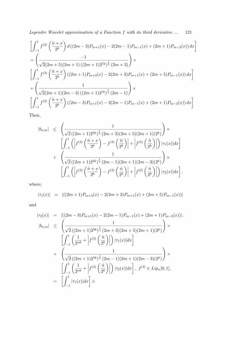
Legendre Wavelet approximation of a Function f with its third derivative ... 121[∫ 1
−1f (2)
(n+ x
2k
)d ((2m− 3)Pm+1(x)− 2(2m− 1)Pm−1(x) + (2m+ 1)Pm−3(x)) dx
]=
(−1
√2(2m+ 5)(2m+ 1) ((2m+ 1)27k)
12 (2m+ 3)
)×[∫ 1
−1f (3)
(n+ x
2k
)((2m+ 1)Pm+3(x)− 2(2m+ 3)Pm+1(x) + (2m+ 5)Pm−1(x)) dx
]+
(1
√2(2m+ 1)(2m− 3) ((2m+ 1)27k)
12 (2m− 1)
)×[∫ 1
−1f (3)
(n+ x
2k
)((2m− 3)Pm+1(x)− 2(2m− 1)Pm−1(x) + (2m+ 1)Pm−3(x)) dx
]Then,
|bn,m| ≤
(1
√2 ((2m+ 1)25k)
12 (2m+ 3)(2m+ 5)(2m+ 1)(2k)
)×[∫ 1
−1
(∣∣∣∣f (3)( n+ x
2k
)− f (3)
(n
2k
)∣∣∣∣+
∣∣∣∣f (3)( n
2k
)∣∣∣∣) |τ1(x)|dx]
+
(1
√2 ((2m+ 1)25k)
12 (2m− 1)(2m+ 1)(2m− 3)(2k)
)×[∫ 1
−1
(∣∣∣∣f (3)( n+ x
2k
)− f (3)
(n
2k
)∣∣∣∣+
∣∣∣∣f (3)( n
2k
)∣∣∣∣) |τ2(x)|dx].
where,
|τ1(x)| = |((2m+ 1)Pm+3(x)− 2(2m+ 3)Pm+1(x) + (2m+ 5)Pm−1(x))|
and
|τ2(x)| = |((2m− 3)Pm+1(x)− 2(2m− 1)Pm−1(x) + (2m+ 1)Pm−3(x))| .
|bn,m| ≤
(1
√2 ((2m+ 1)25k)
12 (2m+ 3)(2m+ 5)(2m+ 1)(2k)
)×[∫ 1
−1
(1
2αk+
∣∣∣∣f (3)( n
2k
)∣∣∣∣) |τ1(x)|dx]
+
(1
√2 ((2m+ 1)25k)
12 (2m− 1)(2m+ 1)(2m− 3)(2k)
)×[∫ 1
−1
(1
2αk+
∣∣∣∣f (3)( n
2k
)∣∣∣∣) |τ2(x)|dx], f (3) ∈ Lipα[0, 1],
=
[∫ 1
−1|τ1(x)|dx
]×
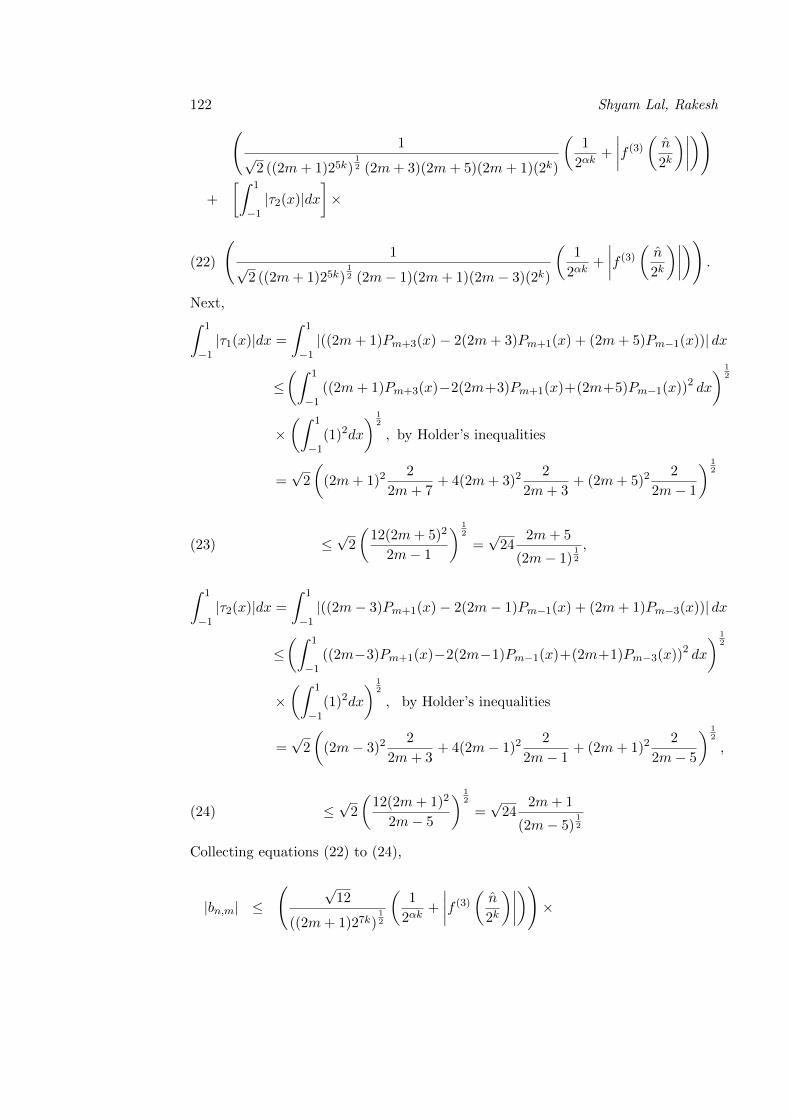
122 Shyam Lal, Rakesh(1
√2 ((2m+ 1)25k)
12 (2m+ 3)(2m+ 5)(2m+ 1)(2k)
(1
2αk+
∣∣∣∣f (3)( n
2k
)∣∣∣∣))
+
[∫ 1
−1|τ2(x)|dx
]×
(22)
(1
√2 ((2m+ 1)25k)
12 (2m− 1)(2m+ 1)(2m− 3)(2k)
(1
2αk+
∣∣∣∣f (3)( n
2k
)∣∣∣∣)).
Next,∫ 1
−1|τ1(x)|dx =
∫ 1
−1|((2m+ 1)Pm+3(x)− 2(2m+ 3)Pm+1(x) + (2m+ 5)Pm−1(x))| dx
≤(∫ 1
−1((2m+ 1)Pm+3(x)−2(2m+3)Pm+1(x)+(2m+5)Pm−1(x))2 dx
) 12
×(∫ 1
−1(1)2dx
) 12
, by Holder’s inequalities
=√
2
((2m+ 1)2
2
2m+ 7+ 4(2m+ 3)2
2
2m+ 3+ (2m+ 5)2
2
2m− 1
) 12
(23) ≤√
2
(12(2m+ 5)2
2m− 1
) 12
=√
242m+ 5
(2m− 1)12
,
∫ 1
−1|τ2(x)|dx =
∫ 1
−1|((2m− 3)Pm+1(x)− 2(2m− 1)Pm−1(x) + (2m+ 1)Pm−3(x))| dx
≤(∫ 1
−1((2m−3)Pm+1(x)−2(2m−1)Pm−1(x)+(2m+1)Pm−3(x))2 dx
) 12
×(∫ 1
−1(1)2dx
) 12
, by Holder’s inequalities
=√
2
((2m− 3)2
2
2m+ 3+ 4(2m− 1)2
2
2m− 1+ (2m+ 1)2
2
2m− 5
) 12
,
(24) ≤√
2
(12(2m+ 1)2
2m− 5
) 12
=√
242m+ 1
(2m− 5)12
Collecting equations (22) to (24),
|bn,m| ≤
( √12
((2m+ 1)27k)12
(1
2αk+
∣∣∣∣f (3)( n
2k
)∣∣∣∣))×
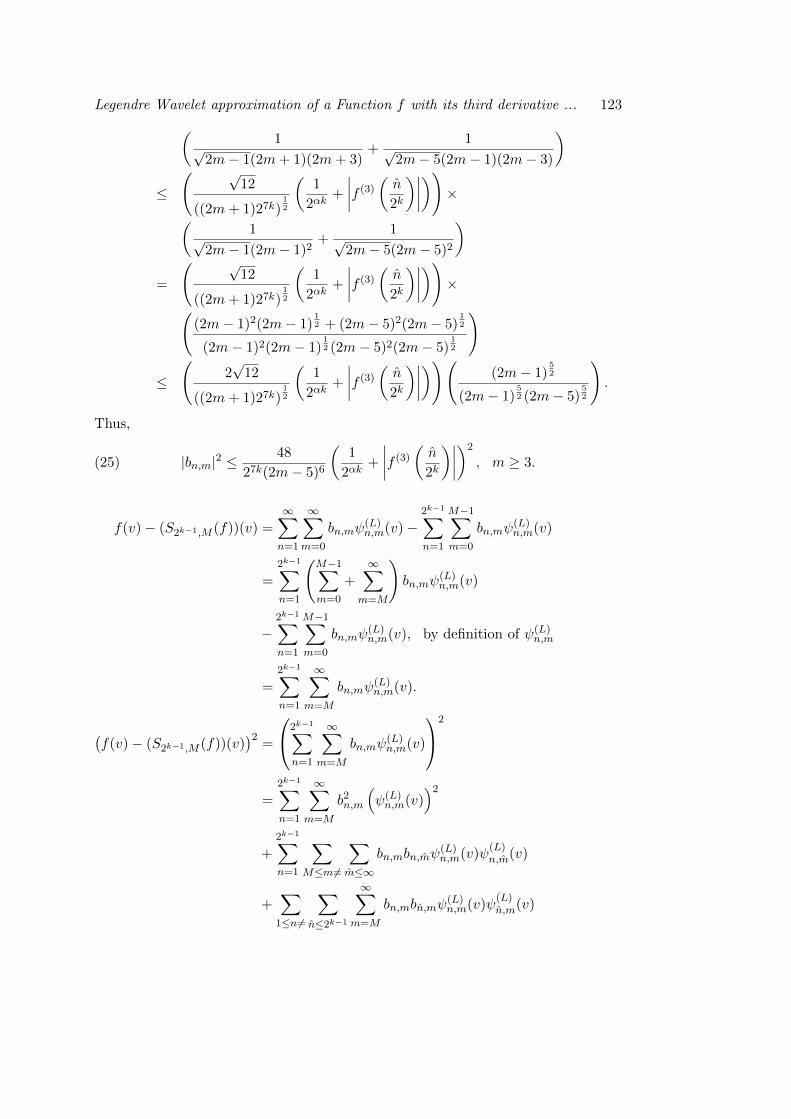
Legendre Wavelet approximation of a Function f with its third derivative ... 123(1√
2m− 1(2m+ 1)(2m+ 3)+
1√2m− 5(2m− 1)(2m− 3)
)≤
( √12
((2m+ 1)27k)12
(1
2αk+
∣∣∣∣f (3)( n
2k
)∣∣∣∣))×(
1√2m− 1(2m− 1)2
+1√
2m− 5(2m− 5)2
)=
( √12
((2m+ 1)27k)12
(1
2αk+
∣∣∣∣f (3)( n
2k
)∣∣∣∣))×(
(2m− 1)2(2m− 1)12 + (2m− 5)2(2m− 5)
12
(2m− 1)2(2m− 1)12 (2m− 5)2(2m− 5)
12
)
≤
(2√
12
((2m+ 1)27k)12
(1
2αk+
∣∣∣∣f (3)( n
2k
)∣∣∣∣))(
(2m− 1)52
(2m− 1)52 (2m− 5)
52
).
Thus,
(25) |bn,m|2 ≤48
27k(2m− 5)6
(1
2αk+
∣∣∣∣f (3)( n
2k
)∣∣∣∣)2
, m ≥ 3.
f(v)− (S2k−1,M (f))(v) =
∞∑n=1
∞∑m=0
bn,mψ(L)n,m(v)−
2k−1∑n=1
M−1∑m=0
bn,mψ(L)n,m(v)
=2k−1∑n=1
(M−1∑m=0
+∞∑
m=M
)bn,mψ
(L)n,m(v)
−2k−1∑n=1
M−1∑m=0
bn,mψ(L)n,m(v), by definition of ψ(L)
n,m
=
2k−1∑n=1
∞∑m=M
bn,mψ(L)n,m(v).
(f(v)− (S2k−1,M (f))(v)
)2=
2k−1∑n=1
∞∑m=M
bn,mψ(L)n,m(v)
2
=2k−1∑n=1
∞∑m=M
b2n,m
(ψ(L)n,m(v)
)2+
2k−1∑n=1
∑M≤m 6=
∑m≤∞
bn,mbn,mψ(L)n,m(v)ψ
(L)n,m(v)
+∑1≤n6=
∑n≤2k−1
∞∑m=M
bn,mbn,mψ(L)n,m(v)ψ
(L)n,m(v)
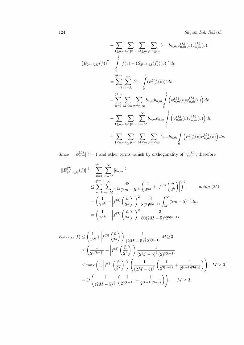
124 Shyam Lal, Rakesh
+∑1≤n6=
∑n≤2k−1
∑M≤m
∑6=m≤∞
bn,mbn,mψ(L)n,m(v)ψ
(L)n,m(v).
(E2k−1,M (f)
)2=
1∫0
∣∣f(v)− (S2k−1,M (f))(v)∣∣2 dv
=2k−1∑n=1
∞∑m=M
b2n,m
1∫0
(ψ(L)n,m(v))2dv
+2k−1∑n=1
∑M≤m
∑6=m≤∞
bn,mbn,m
1∫0
(ψ(L)n,m(v)ψ
(L)n,m(v)
)dv
+∑1≤n6=
∑n≤2k−1
∞∑m=M
bn,mbn,m
1∫0
(ψ(L)n,m(v)ψ
(L)n,m(v)
)dv
+∑1≤n6=
∑n≤2k−1
∑M≤m
∑6=m≤∞
bn,mbn,m
1∫0
(ψ(L)n,m(v)ψ
(L)n,m(v)
)dv.
Since ||ψ(L)n,m||22 = 1 and other terms vanish by orthogonality of ψ
(L)n,m, therefore
||E(2)
2k−1,M(f)||2 =
2k−1∑n=1
∞∑m=M
|bn,m|2
≤2k−1∑n=1
∞∑m=M
48
27k(2m− 5)6
(1
2αk+
∣∣∣∣f (3)( n
2k
)∣∣∣∣)2
, using (25)
=
(1
2αk+
∣∣∣∣f (3)( n
2k
)∣∣∣∣)2 3
8(2)6(k−1)
∫ ∞M
(2m− 5)−6dm
=
(1
2αk+
∣∣∣∣f (3)( n
2k
)∣∣∣∣)2 3
80(2M − 5)526(k−1)
E2k−1,M (f) ≤(
1
2αk+
∣∣∣∣f (3)( n2k)∣∣∣∣) 1
(2M − 5)52 23(k−1)
,M≥3
≤(
1
2α(k−1)+
∣∣∣∣f (3)( n
2k
)∣∣∣∣) 1
(2M − 5)52 (2)3(k−1)
≤ max
(1,
∣∣∣∣f (3)( n
2k
)∣∣∣∣)(
1
(2M − 5)52
(1
23(k−1)+
1
2(k−1)(3+α)
)), M ≥ 3
= O
(1
(2M − 5)52
(1
23(k−1)+
1
2(k−1)(3+α)
)), M ≥ 3.
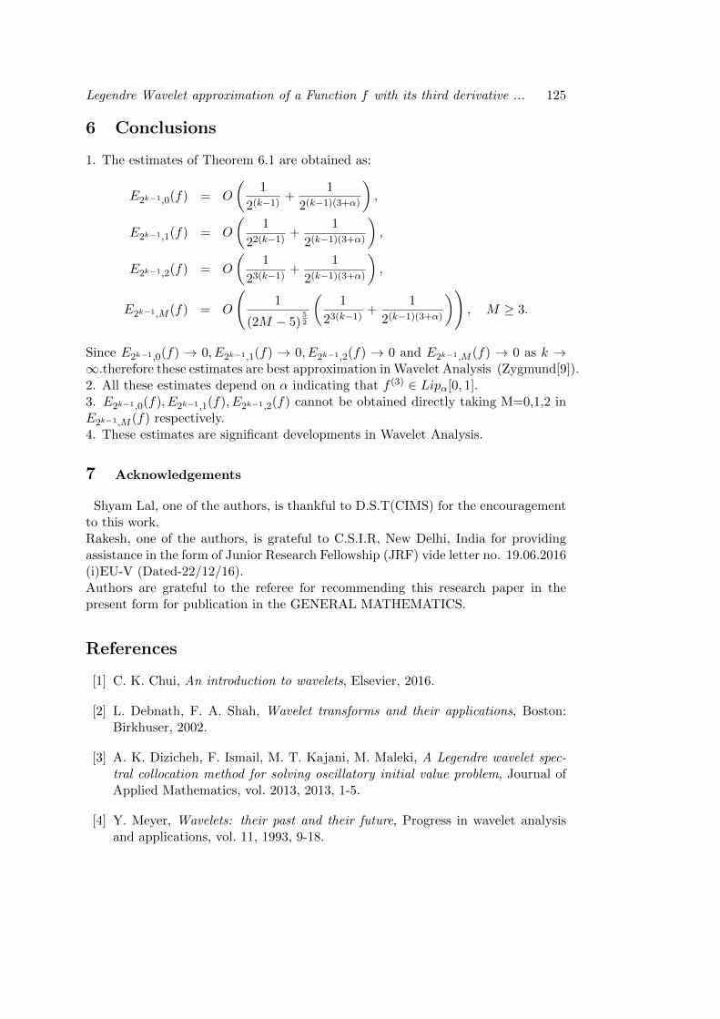
Legendre Wavelet approximation of a Function f with its third derivative ... 125
6 Conclusions
1. The estimates of Theorem 6.1 are obtained as:
E2k−1,0(f) = O
(1
2(k−1)+
1
2(k−1)(3+α)
),
E2k−1,1(f) = O
(1
22(k−1)+
1
2(k−1)(3+α)
),
E2k−1,2(f) = O
(1
23(k−1)+
1
2(k−1)(3+α)
),
E2k−1,M (f) = O
(1
(2M − 5)52
(1
23(k−1)+
1
2(k−1)(3+α)
)), M ≥ 3.
Since E2k−1,0(f) → 0, E2k−1,1(f) → 0, E2k−1,2(f) → 0 and E2k−1,M (f) → 0 as k →∞.therefore these estimates are best approximation in Wavelet Analysis (Zygmund[9]).2. All these estimates depend on α indicating that f (3) ∈ Lipα[0, 1].3. E2k−1,0(f), E2k−1,1(f), E2k−1,2(f) cannot be obtained directly taking M=0,1,2 inE2k−1,M (f) respectively.4. These estimates are significant developments in Wavelet Analysis.
7 Acknowledgements
Shyam Lal, one of the authors, is thankful to D.S.T(CIMS) for the encouragementto this work.Rakesh, one of the authors, is grateful to C.S.I.R, New Delhi, India for providingassistance in the form of Junior Research Fellowship (JRF) vide letter no. 19.06.2016(i)EU-V (Dated-22/12/16).Authors are grateful to the referee for recommending this research paper in thepresent form for publication in the GENERAL MATHEMATICS.
References
[1] C. K. Chui, An introduction to wavelets, Elsevier, 2016.
[2] L. Debnath, F. A. Shah, Wavelet transforms and their applications, Boston:Birkhuser, 2002.
[3] A. K. Dizicheh, F. Ismail, M. T. Kajani, M. Maleki, A Legendre wavelet spec-tral collocation method for solving oscillatory initial value problem, Journal ofApplied Mathematics, vol. 2013, 2013, 1-5.
[4] Y. Meyer, Wavelets: their past and their future, Progress in wavelet analysisand applications, vol. 11, 1993, 9-18.
126 Shyam Lal, Rakesh
[5] J. Morlet, G. Arens, E. Fourgeau, D. Giard, Wave propagation and samplingtheory, part-I, Complex signal and scattering in multilayer media, Geophysics,vol. 47, no. 2, 1982, 203-221.
[6] S. Lal, Rakesh, The approximations of a function belonging Holder classHα[0, 1) by second kind Chebyshev Wavelet Method and applications in solu-tions of differential equation, Accepted for publication in International Journalof Wavelets, Multiresolution and Information Processing, 2018.
[7] S. Lal, Rakesh, Generalized Legendre wavelet method and its applications inapproximation of functions of bounded derivatives, Accepted for publication inPalestine Journal of Mathematics, 2018.
[8] E. C. Titchmarsh, The Theory of functions, Oxford University Press, SecondEdition, 1993.
[9] A. Zygmund , Trigonometric Series, Cambridge University Press, vol. I, 1959.
Dr. Shyam LalBanaras Hindu UniversityProfessorDepartment of MathematicsInstitute of Science, Varanasi-221005, Indiae-mail: shyam [email protected]
RakeshBanaras Hindu UniversityResearch ScholarDepartment of MathematicsInstitute of Science, Varanasi-221005, Indiae-mail: [email protected]
General Mathematics Vol. 26, No. 1-2 (2018), 127–134
Common Coupled Coincidence Point in Cone MetricSpace 1
Krishnadhan Sarkar, Kalishankar Tiwary
Abstract
In this paper we prove some coupled coincidence fixed point theorem inCone metric space with a cone having non-empty interior. Our results is ageneralization of the results of W. Shatanawi[6]. The result generalize manywell known results in the literature.
2010 Mathematics Subject Classification: 47H10, 54H25.Key words and phrases: Common Fixed Point, Coupled fixed point, Coupled
coincidence fixed point, Cone Metric Space.
1 Introduction
In 2007, Huang and Zhang [2] introduce the concept of Cone metric space, replacingthe set of real numbers by an ordered Banach space. They proved some fixed pointtheorems of contractive type mappings over cone metric spaces. Later many authorsgeneralize their fixed point theorems by changing the conditions. V. Bhaskar andLakshmikantam [4] introduced the concept of a coupled fixed point of a mappingF from X × X to X and studied fixed point theorems in partially ordered metricspaces. In 2010, M. Abbas et al.[1] introduce the concept of w-compatible mappingin cone metric spaces and in 2012, W. Shatanawi[6] generalized the results of M.Abbas et al.[1].In this paper we generalize the results of W. Shatanawi [6] by the concept of acommon coupled coincidence point of the mapping F,G : X ×X → X and f : X →X for non-linear contractive mappings in a cone metric space with a cone havingnon-empty interior.
1Received 8 July, 2018Accepted for publication (in revised form) 5 August, 2018
127
128 Krishnadhan Sarkar, Kalishankar Tiwary
2 Preliminarise
2.1 Definition[2]
Let E be a real Banach spaces and K be a subset of E. K is called a cone if andonly if(a). K is closed, nonempty and K 6= 0.(b). ax+ by in K for all x, y in K and a, b ≥ 0.(c). x ∈ K and −x ∈ K ⇒ x = 0⇔ K ∩ (−K) = 0.Consider a cone K ⊂ E. We define a partial ordering ≤ with respect to K byx ≤ y if and only if y− x ∈ K, we write x < y to indicate that x ≤ y but x 6= y andx << y to indicate that y − x ∈ intK. The intK denotes the interior of K.Let X be a non empty set and K ⊂ E be a real Banach space. Suppose the metricmapping d : X ×X → E is satisfies the following conditions:1. d(x, y) ≥ 0 and d(x, y) = 0 iff x = y, for all x, y in X.2. d(x, y) = d(y, x), for all x ,y in X.3. d(x, z) ≤ d(x, y) + d(y, z); for all x,y,z in X.Then d is called a cone metric on X and (X,d) is called a cone metric space.
2.2 Definition[2]
Let, (X,d) be a cone metric space, x ∈ X and xn is a sequence in X. Then1. xn converges to x if for every c ∈ E with 0 << c there is a natural number Nsuch that d(xn, x) << c for all n ≥ N . We shall denote it by limn→∞xn = x or,xn → x.2. xn is a Cauchy sequence , if for every c ∈ E with 0 << c there is a naturalnumber N such that d(xn, xm) ≤ c for all n,m ≥ N .3. (X, d) is a complete cone metric space if every Cauchy sequence is convergent.
2.3 Definition [6]
An element (x, y) ∈ X × X is called a common coupled fixed point of mappingsF : X ×X → X and f : X → X if F (x, y) = fx = x and F (y, x) = fy = y.
2.4 Definition[6]
An element (x, y) ∈ X ×X is called a common coupled coincidence point of map-pings F : X ×X → X and f : X → X if F (x, y) = fx and F (y, x) = fy.
Common Coupled Coincidence Point in Cone Metric Space 129
3 Main Result
3.1 Theorem
Let, (X,d) be a cone metric space with a cone P having nonempty interior. LetF,G : X ×X → X and f : X → X be functions such that
d(F (x, y), G(u, v)) ≤ α1d(fx, fu)+α2d(fy, fv)+α3d(F (x, y), fx)+α4d(G(u, v), fu)
+α5d(F (x, y), fu) + α6d(G(u, v), fx) + α7d(G(u, v), fu) + d(F (x, y), fu)
2
+α8d(fx, fu) + d(F (x, y), fu)
2+ α9
d(F (x, y, fx) + d(F (x, y), fu)
2
(1) +α10d(fx, fu) + d(F (x, y), fx) + d(F (x, y), fu)
3
holds for all x, y, u, v ∈ X. Also F,G and f satiesfy the following conditions:(a) F (X ×X) ⊆ f(X))(b) G(X ×X) ⊆ f(X) and(c) f(X) is a complete subspace of X.If all αi > 0 and (α1 + α2 + α3 + α4 + α5) + 2α6 + α7+α8+α9
2 + 2α103 < 1
Then, F,G and f have a common coupled coincidence point in X.Proof. Let, x0, y0 be two arbitrary elements in X. As, F (X ×X) ⊆ f(X), we canchoose x1, y1 ∈ X such that fx1 = F (x0, y0) and fy1 = F (y0, x0).Again as G(X ×X) ⊆ f(X), we can choose x2, y2 ∈ X such that fx2 = G(x1, y1)and fy2 = G(y1, x1) containing the same process, we can construct two sequences(xn) and (yn) in X such thatfx2n+1 = F (x2n, y2n) and fy2n+1 = F (y2n, x2n); fx2n+2 = G(x2n+1, y2n+1) andfy2n+2 = G(y2n+1, x2n+1)Let,n ∈ N ∪ 0. Then, we have,
d(fx2n, fx2n+1) = d(F (x2n, y2n), G(x2n+1, y2n+1))
≤ α1d(f2n, fx2n+1) + α2d(fy2n, fy2n+1) + α3d(F (x2n, y2n), fx2n)
+α4d(G(x2n+1, y2n+1), fx2n+1) + α5d(F (x2n, y2n), fx2n+1)+
α6d(G(x2n+1, y2n+1), fx2n)+α7d(G(x2n+1, y2n+1), fx2n+1) + d(F (x2n, y2n), fx2n+1)
2
+α8d(fx2n, fx2n+1) + d(F (x2n, y2n), fx2n+1)
2
+α9d(F (x2n, y2n), fx2n) + d(F (x2n, y2n), fx2n+1)
2+
α10d(fx2n, fx2n+1) + d(F (x2n, y2n), fx2n) + d(F (x2n, y2n), fx2n+1)
3
130 Krishnadhan Sarkar, Kalishankar Tiwary
= α1d(fx2n, fx2n+1)+α2d(fy2n, fy2n+1)+α3d(fx2n+1, fx2n)+α4d(fx2n+2, fx2n+1)+
α5d(fx2n+1, fx2n+1)+α6d(fx2n+2, fx2n)+α7d(fx2n+2, fx2n+1) + d(fx2n+1, fx2n+1)
2
+α8d(fx2n, fx2n+1) + d(fx2n+1, fx2n+1)
2+ α9
fx2n+1, fx2n) + d(fx2n+1, fx2n+1)
2
(2) +α10d(fx2n, fx2n+1) + d(fx2n+1, fx2n) + d(fx2n+1, fx2n+1)
3
Again, d(fx2n+2, fx2n) ≤ d(fx2n+2, fx2n+1) + d(fx2n+1, fx2n)So, we get from (2),
(1− α4 − α6 −α7
2)d(fx2n+2, fx2n+1)(3)
≤ (α1 + α3 + α6 +α8
2+α9
2+ 2
α10
3)d(fx2n+1, fx2n) + α2d(fy2n+1, fy2n).
Similarly we will get,
(1− α4 − α6 −α7
2)d(fy2n+2, fy2n+1)(4)
≤ (α1 + α3 + α6 +α8
2+α9
2+ 2
α10
3)d(fy2n+1, fy2n) + α2d(fx2n+1, fx2n).
Adding (3) and (4) we get,
(1− α4 − α6 −α7
2)[d(fx2n+2, fx2n+1) + d(fy2n+2, fy2n+1)]
(5)
≤ (α1 + α2 + α3 + α6 +α8
2+α9
2+ 2
α10
3)[d(fx2n+1, fx2n) + d(fy2n+1, fy2n)].
Let, r =α1 + α2 + α3 + α6 + α8
2 + α92 + 2α10
3
(1− α4 − α6 − α72 )
i.e., r < 1 as
α1 + α2 + α3 + α4 + α5) + 2α6 +α7 + α8 + α9
2+ 2
α10
3< 1
are given. So, from (5) we get,
(6) [d(fx2n+2, fx2n+1)+d(fy2n+2, fy2n+1)] ≤ r[d(fx2n+1, fx2n)+d(fy2n+1, fy2n)].
Similarly, if we proceed then we will get,
(7) [d(fx2n+1, fx2n) + d(fy2n+1, fy2n)] ≤ r[d(fx2n, fx2n−1) + d(fy2n, fy2n−1)].
From inequality (6) and (7) we get,
[d(fx2n+2, fx2n+1) + d(fy2n+2, fy2n+1)] ≤ r[d(fx2n+1, fx2n) + d(fy2n+1, fy2n)]
≤ r2[d(fx2n, fx2n−1) + d(fy2n, fy2n−1)]
≤ ... ≤ r2n+1[d(fx1, fx0) + d(fy1, fy0)].
Common Coupled Coincidence Point in Cone Metric Space 131
Let, (wn)∞n=0 = (fx0, fx1, fx2, ...) and (zn)∞n=0 = (fy0, fy1, fy2, ...) for all n ∈ N ,we have
(8) [d(wn, wn+1) + d(zn, zn+1)] ≤ rn[d(w0, w1) + d(z0, z1)].
Case I: If d(w0, w1) + d(z0, z1) = θ , gives that w0 = w1 and z0 = z1. Byinequality (8), we get w0 = wn and z0 = zn for each n ∈ N . Hence, fx0 = fx1 =F (x0, y0) and fy0 = fy1 = F (y0, x0) Now, we will prove that G(x0, y0) = fx0, andG(y0, x0) = fy0. From given condition we have,
d(fx0, G(x0, y0)) = d(F (x0, y0), G(x0, y0)) ≤ α1d(fx0, fx0) + α2d(fy0, fy0)
+ α3d(fx0, fx0) + α4d(G(x0, y0), fx0) + α5d(fx0, fx0)
+ α6d(G(x0, y0), fx0) + α7d(G(x0, y0), fx0) + d(fx0, fx0)
2
+ α8d(fx0, fx0) + d(fx0, fx0)
2+ α9
d(fx0, fx0) + d(fx0, fx0)
2
+ α10d(fx0, fx0) + d(fx0, fx0) + d(fx0, fx0)
3.
Or, d(fx0, G(x0, y0)) ≤ (α4 +α6 + α72 )d(fx0, G(x0, y0)). Since, α4 +α6 + α7
2 < 1, weget, d(fx0, G(x0, y0)) = θ. And hence, fx0 = G(x0, y0) . Similarly, we can show thatfy0 = G(y0, x0). So, we get that the point (x0, y0) is a common coupled coincidencepoint of F, G and f.
Case II: If d(w0, w1) + d(z0, z1) 6= θ. For, m > n we get
d(wn, wm) ≤ d(wn, wn+1) + ...+ d(wm−1, wm)
andd(zn, zm) ≤ d(zn, zn+1) + ...+ d(zm−1, zm).
By inequality (8) and from r < 1 , we have
d(wn, wm) + d(zn, zm) ≤ rn
1− r[d(w0, w1) + d(z0, z1)]→ θ as n→∞.
Thus for c >> θ , we can find k ∈ N such that
rn
1− r[d(w0, w1) + d(z0, z1)] << c for all n ≥ k.
Hence,d(wn, wm) + d(zn, zm) << c, for all n ≥ k.
Since, d(wn, wm) ≤ d(wn, wm) + d(zn, zm) and d(zn, zm) ≤ d(wn, wm) + d(zn, zm).Now, we can say that (wn) and (zn) are Cauchy sequences in f(X). As f(X) iscomplete,we can find x,y in X such that
wn = f(xn)→ f(x)
132 Krishnadhan Sarkar, Kalishankar Tiwary
and
zn = f(yn)→ f(y) as n→∞.
So, we have f(x2n+1)→ f(x), f(x2n)→ f(x) and f(y2n+1)→ f(y) , f(y2n)→ f(y).
We will prove that F (x, y) = G(x, y) = fx and F (y, x) = G(y, x) = fy.
Now,
(9) d(F (x, y), fx) ≤ d(F (x, y), fx2n+2) + d(fx2n+2, fx),
d(F (x, y), fx2n+2) = d(F (x, y), G(x2n+1, y2n+1))
(10)
≤ α1d(fx, fx2n+1) + α2d(fy, fy2n+1) + α3d(F (x, y), fx) + α4d(fx2n+2, fx2n+1)
+α5d(F (x, y), fx2n+1)+α6d(fx2n+1, fx)+α7d(fx2n+2, fx2n+1)+d(F (x, y), fx2n+1)
2
+ α8d(fx, fx2n+1) + d(F (x, y), fx2n+1)
2+ α9
d(F (x, y), fx) + d(F (x, y), fx2n+1)
2
+ α10d(fx, fx2n+1) + d(F (x, y), fx) + d(F (x, y), fx2n+1)
3.
Put,
d(fx2n+2, fx2n+1) ≤ d(fx2n+2, fx) + d(fx, fx2n+1)
and
d(F (x, y), fx2n+1) ≤ d(F (x, y), fx) + d(fx, fx2n+2).
So, from (10) we get,
(1− α3 − α5 − α9 −α7 + α8
2− 2
α10
3)d(F (x, y), fx) ≤ α2d(fy, fy2n+1)+
(α1+α4+α5+α7+α8+α9
2+2
α10
3)d(fx, fx2n+1)+(α4+α6+
α7
2)d(fx, fx2n+2).
So,
d(F (x, y), fx) ≤ α2
(1− α3 − α5 − α9 − α7+α82 − 2α10
3 )d(fy, fy2n+1)(11)
+(α1 + α4 + α5 + α7 + α8 + +α9
2 + 2α103 )
(1− α3 − α5 − α9 − α7+α82 − 2α10
3 )d(fx, fx2n+1)
+(α4 + α6 + α7
2 )
(1− α3 − α5 − α9 − α7+α82 − 2α10
3 )d(fx, fx2n+2).
Since, f(x2n+1) → f(x), f(x2n) → f(x) and f(y2n+1) → f(y) , f(y2n) → f(y) asn→∞, then for c >> θ there is N0 ∈ N such that
d(fy, fy2n+1) ≤(1− α3 − α5 − α9 − α7+α8
2 − 2α103 )
3α2c
Common Coupled Coincidence Point in Cone Metric Space 133
d(fx, fx2n+1) ≤(1− α3 − α5 − α9 − α7+α8
2 − 2α103 )
3(α1 + α4 + α5 + α7 + α8 + α92 + 2α10
3 )c
and
d(fx, fx2n+2) ≤(1− α3 − α5 − α9 − α7+α8
2 − 2α103 )
3(α4 + α6 + α72 )
c
hold for all n ≥ N . So, d(F (x, y), fx) << c and hence, F (x, y) = fx.Similarly, if we proceed as above and using the inequality:
d(fx,G(x, y)) ≤ d(fx, fx2n+1) + d(fx2n+1, G(x, y))
= d(fx2n+1, fx) + d(F (x2n, y2n), G(x, y))
we will get, G(x, y) = fx . Hence, F (x, y) = G(x, y) = fx. By using the samemethod as above we can show that F (y, x) = G(y, x) = fy . Therefore, (x, y) is acommon coupled coincidence point of the mappings F,G and f.
3.2 Theorem
Let, (X,d) be a cone metric space with a cone P having nonempty interior. LetF : X ×X → X and f : X → X be functions such that
d(F (x, y), F (u, v)) ≤ α1d(fx, fu) + α2d(fy, fv) + α3d(F (x, y), fx) + α4d(F (u, v), fu)
(12)
+ α5d(F (x, y), fu) + α6d(F (u, v), fx) + α7d(F (u, v), fu) + d(F (x, y), fu)
2
+ α8d(fx, fu) + d(F (x, y), fu)
2+ α9
d(F (x, y, fx) + d(F (x, y), fu)
2
+ α10d(fx, fu) + d(F (x, y), fx) + d(F (x, y), fu)
3.
holds for all x, y, u, v ∈ X. Also F and f satiesfy the following conditions:(a) F (X ×X) ⊆ f(X)).(b) f(X) is a complete subspace of X.If all αi > 0 and (α1 + α2 + α3 + α4 + α5) + 2α6 + α7+α8+α9
2 + 2α103 < 1.
Then, F and f have a common coupled coincidence point in X.Proof. Put G = F in Theorem 3.1, then we will get the required result.
4 Conclusion
If we put α7 = α8 = α9 = α10 = 0 and α5 = α4 and α6 = α5 in our main result ,then we get the results of W. Shatanawi [6]. Our main result is a generalization ofmany results in the literature.
134 Krishnadhan Sarkar, Kalishankar Tiwary
References
[1] M. Abbas et al., Common coupled fixed point theorems in cone metric spacefor w-compatible mapping, Applied Mathematics and Computation, 2010, doi:10.1016/j.amc.2010.05.042.
[2] L. G. Haung, X. Zhang, Cone metric space and fixed point theorems of contrac-tive mappings, Journal of Mathematical Analysis and Applications, vol. 332,2007, 1468-1476.
[3] E. Karapinar, Couple Fixed Point on Cone Metric spaces, Gazi University Jour-nal of Science, vol. 24, no. 1, 2011, 51-58.
[4] V. Lakshmikantham, Lj. B. Ciric, Coupled fixed point theorems for nonlinearcontractions in partially ordered metric spaces, Nonlinear Analysis, vol. 70,2009, 4341-4349.
[5] W. Shatanawi, Some Common Coupled Fixed Point Results in Cone MetricSpaces, Int. Journal of Math. Analysis, vol. 4, no. 48, 2010, 2381-2388.
[6] W. Shatanawi, On w-compatible mappings and common coupled coincidencepoint in cone metric spaces, Applied Mathematics Letters, vol. 25, 2012, 925-931.
Krishnadhan SarkarRaniganj Girls’ CollegeAssistant ProfessorDepartment of MathematicsRaniganj-713358, Westbengal, Indiae-mail: [email protected]
Kalishankar TiwaryRaiganj UniversityProfessorDepartment of MathematicsRaiganj-733134, West Bengal, Indiae-mail: [email protected]