Helicopter Loads Synthesis using a Neural Network Abstract · Helicopter Loads Synthesis using a Neural Network C. Cheung*, L. Krake† Abstract This study investigates the use of

AIAC-12 Twelfth Australian International Aerospace Congress

Fifth DSTO International Conference on Health & Usage Monitoring – HUMS2007

Helicopter Loads Synthesis using a Neural Network C. Cheung*, L. Krake†

Abstract

This study investigates the use of a multi-layer artificial neural network (ANN) to estimate helicopter dynamic component loads from fixed airframe measurements using data obtained from a S-70A-9 Black Hawk flight loads survey. While measuring dynamic component loads directly is possible through slip-rings or telemetry systems, these methods are not reliable and are difficult to maintain. The estimation of dynamic component loads based on fixed airframe measurements would be significantly more practical and efficient. The goal of this work is to assess the effectiveness of neural networks to estimate these loads, and thereby obtain more accurate loads data sets, that would enable the calculation of more accurate component retirement times (CRTs). It has been shown that small changes in flight loads can result in extremely large changes in the calculated fatigue lives of components [1]. Since CRTs are a major driver of maintenance and replacement costs, more accurate estimates of the component lives would enable the fatigue life management of a helicopter fleet to be significantly improved. This paper provides the initial implementation details of the neural network and the preliminary results obtained demonstrating the method validity and its potential as an effective and accurate tool in addressing this issue.

Keywords: helicopter, load synthesis, Black Hawk, neural network.

Abbreviations ANN CRT ESSS FDR FFT FS IFFT MR NR TR VH

artificial neural network component retirement time External Stores Support System flight data recorder fast fourier transform fuselage station inverse FFT main rotor normal rotor speed tail rotor maximum level flight indicated airspeed achievable at max continuous engine power

1. Introduction

Accurately determining component loads on a helicopter is an important goal in the helicopter structural integrity field. These loads are used to calculate the component retirement times (CRTs) that indicate the number of flight hours a component can safely be used in service. Once a component has reached this point it must be discarded. One of the factors that aircraft manufacturers use to define CRTs is the design usage spectrum. This usage spectrum is meant to be a worst-case scenario for how the aircraft will be used in * Research Officer, Institute for Aerospace Research, National Research Council Canada, Ottawa, Canada. [email protected]. † Helicopter Structural Engineer, Air Vehicles Division, Defence Science and Technology Organisation, Melbourne, Australia.


Fifth DSTO International Conference on Health & Usage Monitoring – HUMS2007 2

service. Hence, this usage spectrum will be different to how operators actually use the aircraft. An operator may elect to determine and apply a new usage spectrum for their fleet, however, this spectrum still be based on the worst aspects of the intended usage, and not how they are actually flown.

The rotor system components and attachments are some of the most fatigue-critical structural components on a helicopter. Direct measurement of the dynamic loads in these areas has traditionally been accomplished through slip rings or telemetry systems, however, these techniques are difficult to implement and are often unreliable. Over the past few decades, there have been a number of attempts at estimating these dynamic component loads indirectly from loads measured at fixed points on the airframe or from flight state parameters recorded by a flight data recorder (FDR). Ref. 2 summarises the major findings in this area up until the late 1990s.

Figure 1: Australian Army Black Hawk S-70-A-9

In this work, the data gathered from a Sikorsky Black Hawk S-70A-9 operated by the Australian Army (Figure 1) were analysed. In common with other helicopter manufacturers, Sikorsky uses three key elements to calculate component fatigue lives from which the recommended CRTs are specified. These elements are: the usage spectrum, flight load data, and fatigue strength data [1]. The usage spectrum lists a set of flight conditions and quantifies the expected worst case usage for the aircraft during its service life. In addition, the usage spectrum attributes a percentage of the total flight time expected to be spent in each of these flight regimes. The flight load data define the expected loads on components during each flight regime. Finally, the fatigue strength data, often obtained by material coupon testing, show the degree of resistance of a particular material or component to fatigue damage from the flight loads, i.e. the number of cycles at a particular cyclic stress level the material or component will endure.

Obtaining accurate loads data relevant to the actual usage of the aircraft is extremely important. It has been shown that small changes in the flight loads values or material strength data can translate to drastic changes in a component’s calculated fatigue life [1]. Hence, helicopter manufacturers must apply very conservative assumptions to their loads data to ensure that errors in measuring loads do not result in non-conservative CRTs. This work focuses on developing an effective method to determine flight loads more accurately. This paper describes the implementation details of a neural network used to estimate the dynamic loads in the main rotor.

2. Test data

The data used in this work was obtained from a S-70A-9 Black Hawk flight loads survey conducted in 2000 by the Georgia Tech Research Institute (GTRI) on behalf of the United



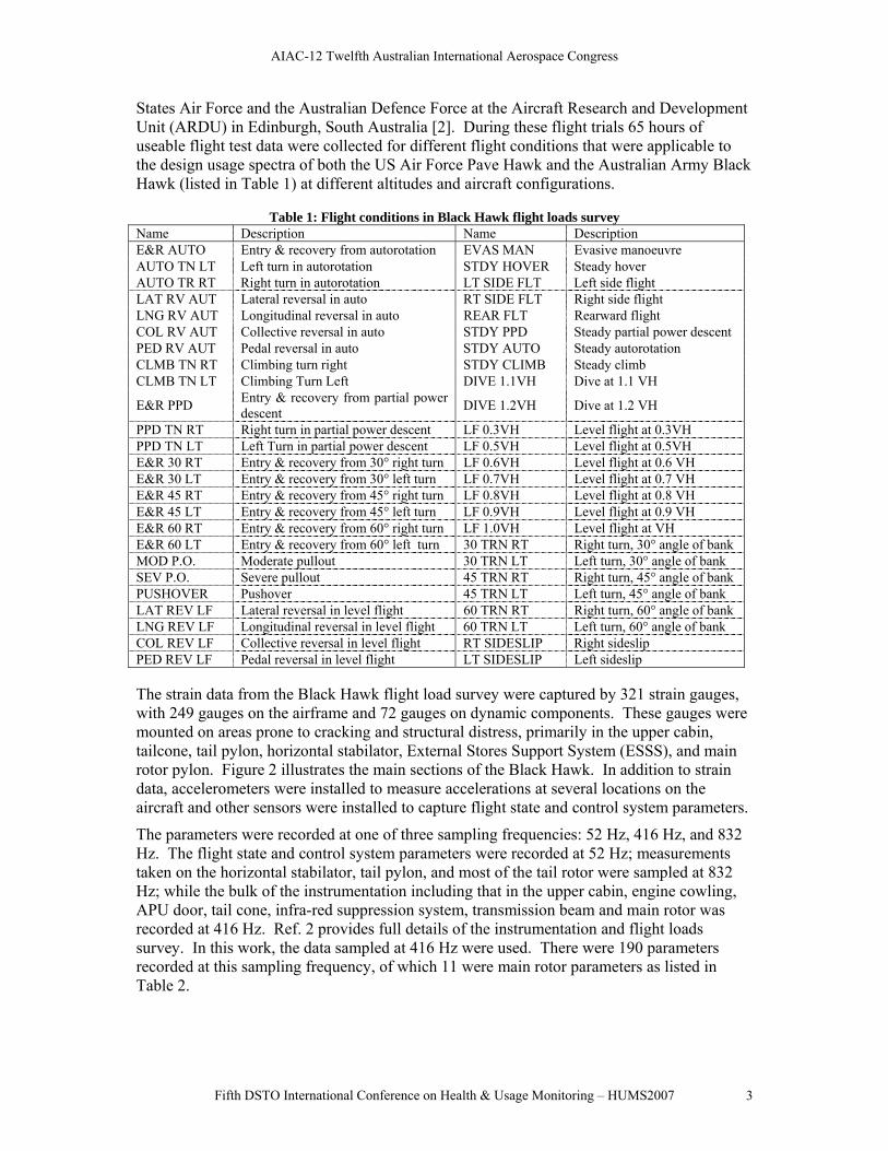
States Air Force and the Australian Defence Force at the Aircraft Research and Development Unit (ARDU) in Edinburgh, South Australia [2]. During these flight trials 65 hours of useable flight test data were collected for different flight conditions that were applicable to the design usage spectra of both the US Air Force Pave Hawk and the Australian Army Black Hawk (listed in Table 1) at different altitudes and aircraft configurations.

Table 1: Flight conditions in Black Hawk flight loads survey Name Description Name Description E&R AUTO Entry & recovery from autorotation EVAS MAN Evasive manoeuvre AUTO TN LT Left turn in autorotation STDY HOVER Steady hover AUTO TR RT Right turn in autorotation LT SIDE FLT Left side flight LAT RV AUT Lateral reversal in auto RT SIDE FLT Right side flight LNG RV AUT Longitudinal reversal in auto REAR FLT Rearward flight COL RV AUT Collective reversal in auto STDY PPD Steady partial power descent PED RV AUT Pedal reversal in auto STDY AUTO Steady autorotation CLMB TN RT Climbing turn right STDY CLIMB Steady climb CLMB TN LT Climbing Turn Left DIVE 1.1VH Dive at 1.1 VH

E&R PPD Entry & recovery from partial power descent DIVE 1.2VH Dive at 1.2 VH

PPD TN RT Right turn in partial power descent LF 0.3VH Level flight at 0.3VH PPD TN LT Left Turn in partial power descent LF 0.5VH Level flight at 0.5VH E&R 30 RT Entry & recovery from 30° right turn LF 0.6VH Level flight at 0.6 VH E&R 30 LT Entry & recovery from 30° left turn LF 0.7VH Level flight at 0.7 VH E&R 45 RT Entry & recovery from 45° right turn LF 0.8VH Level flight at 0.8 VH E&R 45 LT Entry & recovery from 45° left turn LF 0.9VH Level flight at 0.9 VH E&R 60 RT Entry & recovery from 60° right turn LF 1.0VH Level flight at VH E&R 60 LT Entry & recovery from 60° left turn 30 TRN RT Right turn, 30° angle of bank MOD P.O. Moderate pullout 30 TRN LT Left turn, 30° angle of bank SEV P.O. Severe pullout 45 TRN RT Right turn, 45° angle of bank PUSHOVER Pushover 45 TRN LT Left turn, 45° angle of bank LAT REV LF Lateral reversal in level flight 60 TRN RT Right turn, 60° angle of bank LNG REV LF Longitudinal reversal in level flight 60 TRN LT Left turn, 60° angle of bank COL REV LF Collective reversal in level flight RT SIDESLIP Right sideslip PED REV LF Pedal reversal in level flight LT SIDESLIP Left sideslip

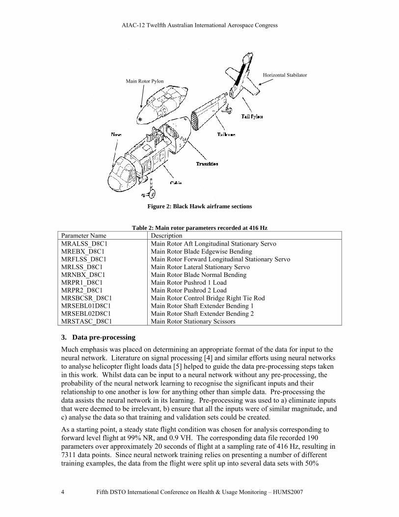
The strain data from the Black Hawk flight load survey were captured by 321 strain gauges, with 249 gauges on the airframe and 72 gauges on dynamic components. These gauges were mounted on areas prone to cracking and structural distress, primarily in the upper cabin, tailcone, tail pylon, horizontal stabilator, External Stores Support System (ESSS), and main rotor pylon. Figure 2 illustrates the main sections of the Black Hawk. In addition to strain data, accelerometers were installed to measure accelerations at several locations on the aircraft and other sensors were installed to capture flight state and control system parameters.

The parameters were recorded at one of three sampling frequencies: 52 Hz, 416 Hz, and 832 Hz. The flight state and control system parameters were recorded at 52 Hz; measurements taken on the horizontal stabilator, tail pylon, and most of the tail rotor were sampled at 832 Hz; while the bulk of the instrumentation including that in the upper cabin, engine cowling, APU door, tail cone, infra-red suppression system, transmission beam and main rotor was recorded at 416 Hz. Ref. 2 provides full details of the instrumentation and flight loads survey. In this work, the data sampled at 416 Hz were used. There were 190 parameters recorded at this sampling frequency, of which 11 were main rotor parameters as listed in Table 2.



Figure 2: Black Hawk airframe sections

Table 2: Main rotor parameters recorded at 416 Hz Parameter Name Description MRALSS_D8C1 MREBX_D8C1 MRFLSS_D8C1 MRLSS_D8C1 MRNBX_D8C1 MRPR1_D8C1 MRPR2_D8C1 MRSBCSR_D8C1 MRSEBL01D8C1 MRSEBL02D8C1 MRSTASC_D8C1

Main Rotor Aft Longitudinal Stationary Servo Main Rotor Blade Edgewise Bending Main Rotor Forward Longitudinal Stationary Servo Main Rotor Lateral Stationary Servo Main Rotor Blade Normal Bending Main Rotor Pushrod 1 Load Main Rotor Pushrod 2 Load Main Rotor Control Bridge Right Tie Rod Main Rotor Shaft Extender Bending 1 Main Rotor Shaft Extender Bending 2 Main Rotor Stationary Scissors

3. Data pre-processing

Much emphasis was placed on determining an appropriate format of the data for input to the neural network. Literature on signal processing [4] and similar efforts using neural networks to analyse helicopter flight loads data [5] helped to guide the data pre-processing steps taken in this work. Whilst data can be input to a neural network without any pre-processing, the probability of the neural network learning to recognise the significant inputs and their relationship to one another is low for anything other than simple data. Pre-processing the data assists the neural network in its learning. Pre-processing was used to a) eliminate inputs that were deemed to be irrelevant, b) ensure that all the inputs were of similar magnitude, and c) analyse the data so that training and validation sets could be created.

As a starting point, a steady state flight condition was chosen for analysis corresponding to forward level flight at 99% NR, and 0.9 VH. The corresponding data file recorded 190 parameters over approximately 20 seconds of flight at a sampling rate of 416 Hz, resulting in 7311 data points. Since neural network training relies on presenting a number of different training examples, the data from the flight were split up into several data sets with 50%

Main Rotor Pylon Horizontal Stabilator



overlap. Each set contained approximately 2 seconds of data, allowing for 14 data sets. Sixty percent of the data sets (9 sets) were used for training, while the remaining sets were reserved for validation purposes.

Since the parameter signals are periodic, it was decided to perform the analyses in the frequency domain. The parameter signals were transformed from the time domain to the frequency domain equivalent using Matlab’s built-in fast-fourier transform (FFT) function. The time domain and frequency domain representations are related by the following equations [4]:

( ) ( )

( ) ( )∑

∑−

=

−

=

−

=

=

1

0

/2

1

0

/2

1 N

m

Nmnj

N

n

Nnmj

emXN

nx

enxmX

π

π

The mean strain of these signals was subtracted from the signals before performing a 1024-point FFT on each of the parameters and normalising the resulting frequency components. Following the work of Lombardo [5], the mean strain component plus nine key main rotor and tail rotor frequencies were extracted from the FFTs to represent the parameters and to be used as inputs (Table 3) to the neural network.

Table 3: Selected analysis frequencies Main Rotor or Tail Rotor Harmonic Frequency

0.25 MR 0.5 MR 1 MR 2 MR 3 MR 4 MR 1 TR 8 MR 12 MR

Mean strain

1.075 Hz 2.15 Hz 4.3 Hz 8.6 Hz 12.9 Hz 17.2 Hz 19.8 Hz 34.4 Hz 51.6 Hz

-

3.1 Verification of key FFT frequencies

To verify that the subset of key frequencies was sufficient to produce an acceptable approximation of the original time domain signal, an analysis of the FFT signals was performed.

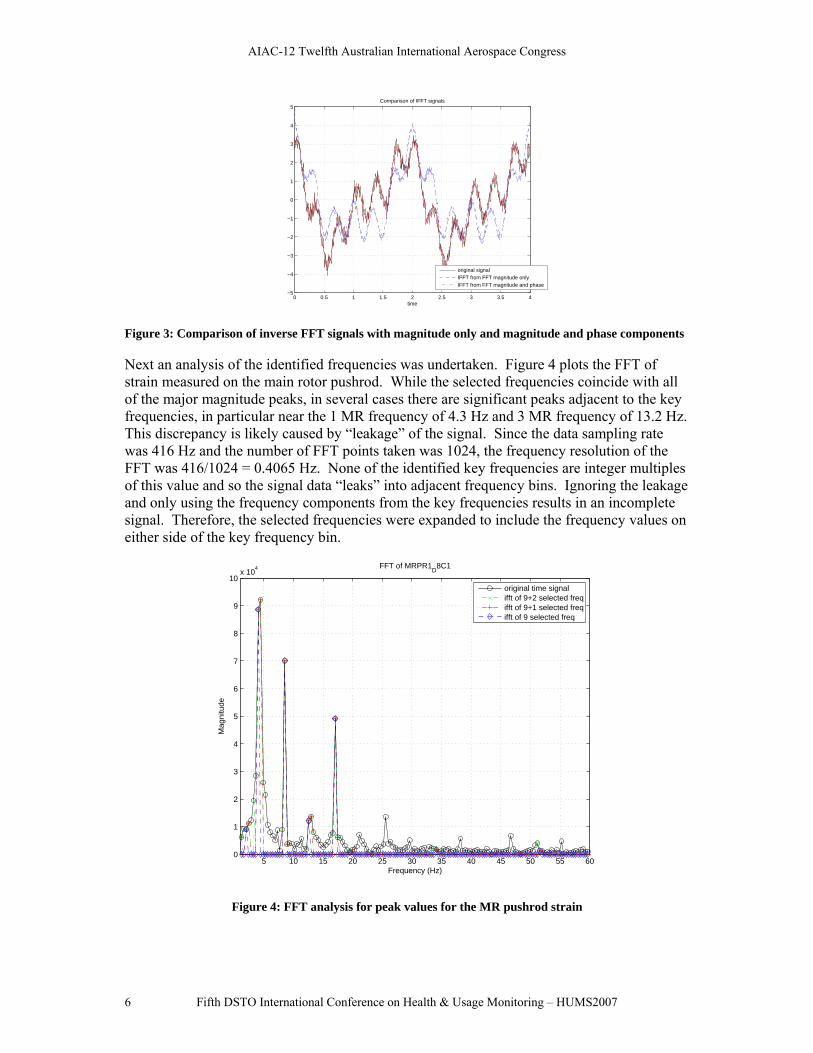
The FFT frequency terms are complex numbers that indicate the magnitude and phase relationship between the FFT frequency and the original signal. While the phase accuracy of the time signal is not considered significant in fatigue damage calculations, amplitudes, peak values, and signal frequency are important. Initially, it was hoped that the magnitude values alone at the selected frequencies would contain enough information to reconstruct the original time sequences. Figure 3 shows a test case evaluating the results of an inverted signal, i.e. the inverse FFT performed on a FFT signal generating its time domain representation, using only magnitude information. While the signal shape is similar, the peak values of the original signal are not reached and therefore the magnitude values alone are insufficient to reconstruct an accurate enough time signal. Thus magnitude and phase components of the FFT signals were required.



0 0.5 1 1.5 2 2.5 3 3.5 4−5

−4

−3

−2

−1

0

1

2

3

4

5

time

Comparison of IFFT signals

original signalIFFT from FFT magnitude onlyIFFT from FFT magnitude and phase

Figure 3: Comparison of inverse FFT signals with magnitude only and magnitude and phase components

Next an analysis of the identified frequencies was undertaken. Figure 4 plots the FFT of strain measured on the main rotor pushrod. While the selected frequencies coincide with all of the major magnitude peaks, in several cases there are significant peaks adjacent to the key frequencies, in particular near the 1 MR frequency of 4.3 Hz and 3 MR frequency of 13.2 Hz. This discrepancy is likely caused by “leakage” of the signal. Since the data sampling rate was 416 Hz and the number of FFT points taken was 1024, the frequency resolution of the FFT was 416/1024 = 0.4065 Hz. None of the identified key frequencies are integer multiples of this value and so the signal data “leaks” into adjacent frequency bins. Ignoring the leakage and only using the frequency components from the key frequencies results in an incomplete signal. Therefore, the selected frequencies were expanded to include the frequency values on either side of the key frequency bin.

5 10 15 20 25 30 35 40 45 50 55 600

1

2

3

4

5

6

7

8

9

10x 10

4 FFT of MRPR1D

8C1

Frequency (Hz)

Mag

nitu

de

original time signalifft of 9+2 selected freqifft of 9+1 selected freqifft of 9 selected freq

Figure 4: FFT analysis for peak values for the MR pushrod strain



0 0.5 1 1.5 2 2.5−6

−5

−4

−3

−2

−1

0

1

2

3x 10

4 Inverse FFT of MREBXD

8C1 using magnitude and phase data

time(s)

stra

in (

µstr

ain)

original time signalifft of 9 selected freqifft of 9+1 selected freqifft of 9+2 selected freq

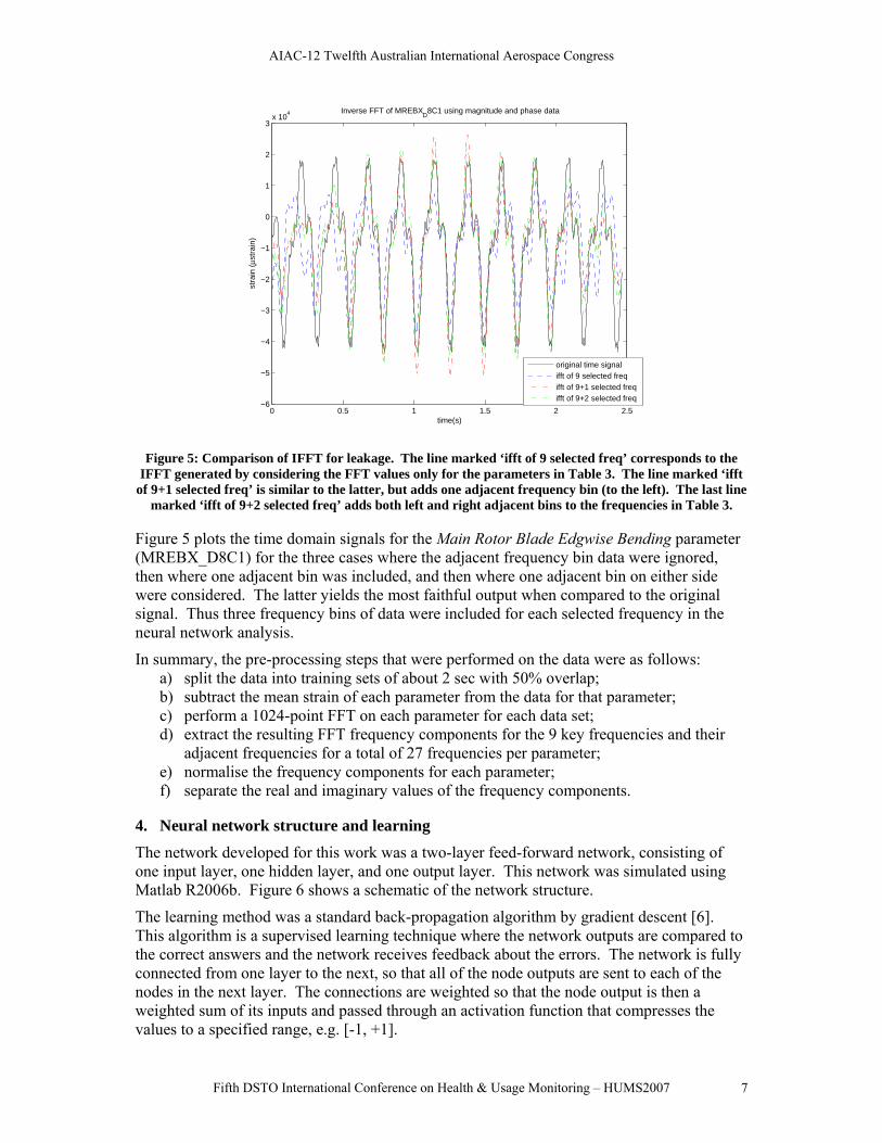
Figure 5: Comparison of IFFT for leakage. The line marked ‘ifft of 9 selected freq’ corresponds to the

IFFT generated by considering the FFT values only for the parameters in Table 3. The line marked ‘ifft of 9+1 selected freq’ is similar to the latter, but adds one adjacent frequency bin (to the left). The last line

marked ‘ifft of 9+2 selected freq’ adds both left and right adjacent bins to the frequencies in Table 3.

Figure 5 plots the time domain signals for the Main Rotor Blade Edgwise Bending parameter (MREBX_D8C1) for the three cases where the adjacent frequency bin data were ignored, then where one adjacent bin was included, and then where one adjacent bin on either side were considered. The latter yields the most faithful output when compared to the original signal. Thus three frequency bins of data were included for each selected frequency in the neural network analysis.

In summary, the pre-processing steps that were performed on the data were as follows: a) split the data into training sets of about 2 sec with 50% overlap; b) subtract the mean strain of each parameter from the data for that parameter; c) perform a 1024-point FFT on each parameter for each data set; d) extract the resulting FFT frequency components for the 9 key frequencies and their

adjacent frequencies for a total of 27 frequencies per parameter; e) normalise the frequency components for each parameter; f) separate the real and imaginary values of the frequency components.

4. Neural network structure and learning

The network developed for this work was a two-layer feed-forward network, consisting of one input layer, one hidden layer, and one output layer. This network was simulated using Matlab R2006b. Figure 6 shows a schematic of the network structure.

The learning method was a standard back-propagation algorithm by gradient descent [6]. This algorithm is a supervised learning technique where the network outputs are compared to the correct answers and the network receives feedback about the errors. The network is fully connected from one layer to the next, so that all of the node outputs are sent to each of the nodes in the next layer. The connections are weighted so that the node output is then a weighted sum of its inputs and passed through an activation function that compresses the values to a specified range, e.g. [-1, +1].



Figure 6: Two-layer back-propagation neural network

The hyperbolic tangent activation function was used in this work yielding outputs in the range [-1, +1] and given by the following equations:

( )( ) ( )21'

tanhgxgxxg

−=

=

β

β

Explicitly, the network inputs, ξk, are fed through to the hidden layer nodes so that the hidden node input, hj,is

j jk kk

h w ξ=∑ ,

where wjk are the weights between the input layer and hidden layer nodes.

The hidden node output, Vj, results from the activation function g(x) applied to its input,

( )j j jk kk

V g h g w ξ⎛ ⎞= = ⎜ ⎟

⎝ ⎠∑

Similarly, the output unit, Oi, receives an input

i ij jj

h W V=∑ ,

where Wij are the weights between the hidden and output layers. The final output, Oi, is calculated as

( )i i ij jj

O g h g W V⎛ ⎞

= = ⎜ ⎟⎝ ⎠∑

To update the weights, the errors are calculated and propagated back through the network.

The error at the output layer is calculated by comparing the network output, Oi to the desired or target output, ζi.

( )[ ]'i i i ig h Oδ ζ= −

For the hidden layer nodes, the error is calculated as

INPUTS: FFT frequency components

OUTPUT: FFT frequency components of MR parameter

wjk

Wij

δij

δjk



( )1 1'm m m mi i ji j

jg h wδ δ− −= ∑

The weights are then updated as follows: 1

ij ij

m m mij i j

new oldij

w V

w w w

αδ −∆ =

= + ∆,

where α is the learning rate.

Network training consists of this learning process and weight update carried out for each training set or pattern input to the network, where each iteration is known as an epoch, and repeated until an acceptable error is achieved. The error measure used in this work was the sum-squared loss:

( )212 i i

ie Oζ= −∑

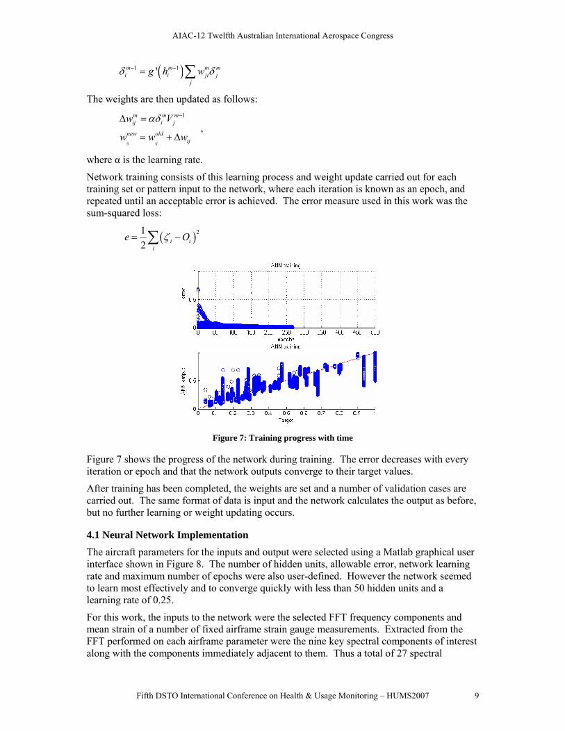
Figure 7: Training progress with time

Figure 7 shows the progress of the network during training. The error decreases with every iteration or epoch and that the network outputs converge to their target values.

After training has been completed, the weights are set and a number of validation cases are carried out. The same format of data is input and the network calculates the output as before, but no further learning or weight updating occurs.

4.1 Neural Network Implementation

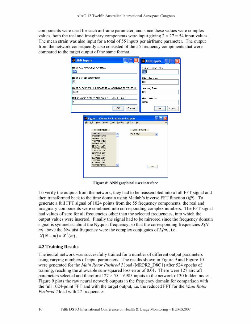
The aircraft parameters for the inputs and output were selected using a Matlab graphical user interface shown in Figure 8. The number of hidden units, allowable error, network learning rate and maximum number of epochs were also user-defined. However the network seemed to learn most effectively and to converge quickly with less than 50 hidden units and a learning rate of 0.25.

For this work, the inputs to the network were the selected FFT frequency components and mean strain of a number of fixed airframe strain gauge measurements. Extracted from the FFT performed on each airframe parameter were the nine key spectral components of interest along with the components immediately adjacent to them. Thus a total of 27 spectral



components were used for each airframe parameter, and since these values were complex values, both the real and imaginary components were input giving 2 × 27 = 54 input values. The mean strain was also input for a total of 55 inputs per airframe parameter. The output from the network consequently also consisted of the 55 frequency components that were compared to the target output of the same format.

Figure 8: ANN graphical user interface

To verify the outputs from the network, they had to be reassembled into a full FFT signal and then transformed back to the time domain using Matlab’s inverse FFT function (ifft). To generate a full FFT signal of 1024 points from the 55 frequency components, the real and imaginary components were combined into corresponding complex numbers. The FFT signal had values of zero for all frequencies other than the selected frequencies, into which the output values were inserted. Finally the signal had to be mirrored since the frequency domain signal is symmetric about the Nyquist frequency, so that the corresponding frequencies X(N-m) above the Nyquist frequency were the complex conjugates of X(m), i.e. ( ) )(* mXmNX =− .

4.2 Training Results

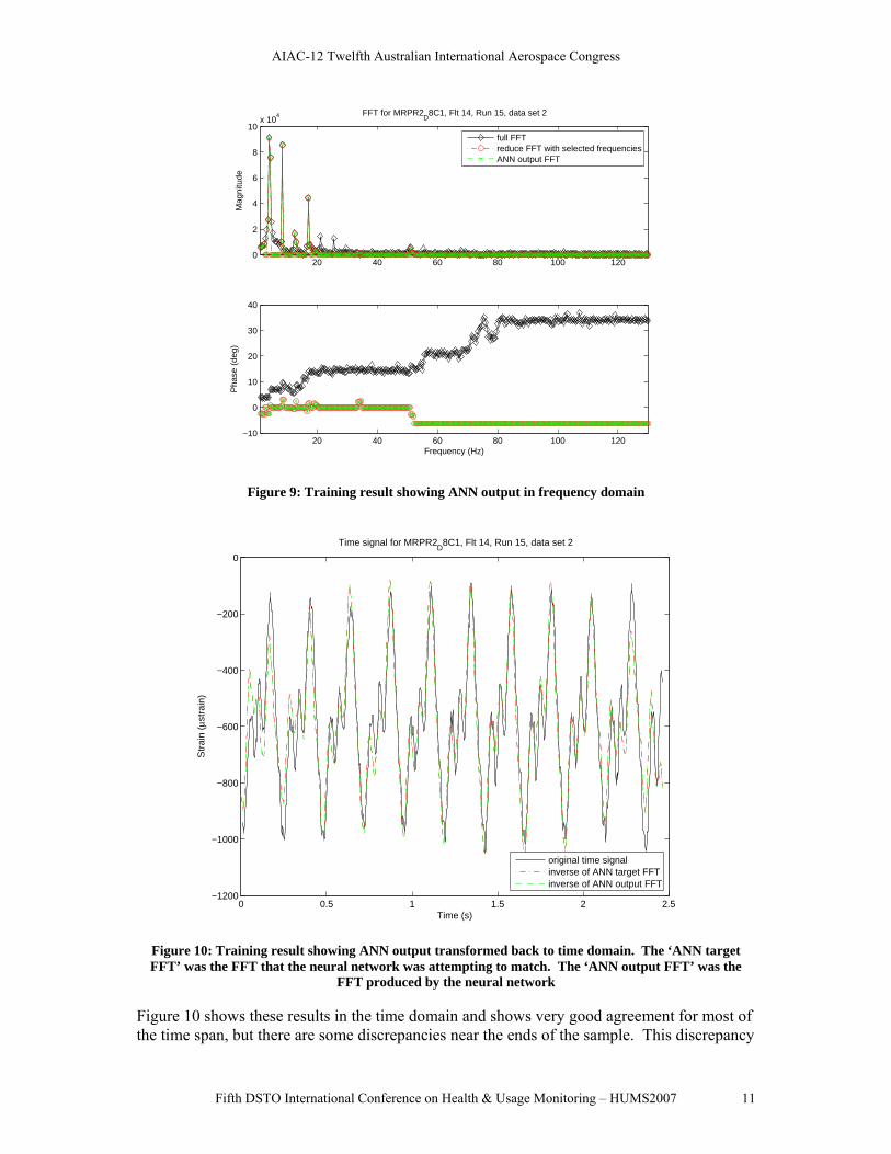
The neural network was successfully trained for a number of different output parameters using varying numbers of input parameters. The results shown in Figure 9 and Figure 10 were generated for the Main Rotor Pushrod 2 load (MRPR2_D8C1) after 524 epochs of training, reaching the allowable sum-squared loss error of 0.01. There were 127 aircraft parameters selected and therefore 127 × 55 = 6985 inputs to the network of 30 hidden nodes. Figure 9 plots the raw neural network outputs in the frequency domain for comparison with the full 1024-point FFT and with the target output, i.e. the reduced FFT for the Main Rotor Pushrod 2 load with 27 frequencies.



20 40 60 80 100 1200

2

4

6

8

10x 10

4 FFT for MRPR2D

8C1, Flt 14, Run 15, data set 2

Mag

nitu

de

full FFTreduce FFT with selected frequenciesANN output FFT

20 40 60 80 100 120−10

0

10

20

30

40

Pha

se (

deg)

Frequency (Hz)

Figure 9: Training result showing ANN output in frequency domain

0 0.5 1 1.5 2 2.5−1200

−1000

−800

−600

−400

−200

0

Time (s)

Str

ain

(µst

rain

)

Time signal for MRPR2D

8C1, Flt 14, Run 15, data set 2

original time signalinverse of ANN target FFTinverse of ANN output FFT

Figure 10: Training result showing ANN output transformed back to time domain. The ‘ANN target FFT’ was the FFT that the neural network was attempting to match. The ‘ANN output FFT’ was the

FFT produced by the neural network

Figure 10 shows these results in the time domain and shows very good agreement for most of the time span, but there are some discrepancies near the ends of the sample. This discrepancy



is likely an artefact of an FFT performed on a finite rectangular window of time. By looking at the results from the preceding and subsequent data sets which overlap by 50%, the same phenomenon is observed. This would confirm that the mismatch is linked to problems with FFTs near the edges of a sample as opposed to problems with the signal itself.

5. Discussion and Future Work

The work described in this paper represents the early stages of an investigation into using neural networks to estimate helicopter dynamic loads. The results thus far demonstrate the validity of the method and highlight its potential to be an effective tool in addressing the issue of estimating dynamic loads from fixed airframe measurements.

The main drawbacks of the current implementation are the large number of inputs used and the loss of accuracy of the output time signal near the edges of the data sample. Minimising the number of inputs required to achieve an accurate output signal will be a major area of focus as this work proceeds. One approach being considered is an automated method to gradually reduce the number of input parameters using a tournament selection scheme or a weights analysis. The airframe parameters will be grouped according to their location on the airframe and a limited number of parameters from each group will be selected based on the magnitudes of their weights. Additionally, using windowing techniques to decrease the leakage of the frequency data into adjacent bins will be explored to reduce the number of frequencies required for each airframe parameter. More research into the sampling effects near the ends of the data samples is likely to improve the fidelity of the estimation of the target parameter at the sample edges. In addition, the ability of the network to adapt to different flight conditions will need to be addressed in the future.

Now that the network has been set up and its overall functionality verified, a series of trials will be conducted on the current data file. These trials will then be extended to other data files of the same flight condition, i.e. forward level flight, 99% NR, 0.9VH. This will then be followed by analysing other flight conditions, however, in the short term, the application of the neural network will be focussed on steady state flight conditions for simplicity.

Acknowledgments

This work was undertaken with the aid and support of the Helicopter Structural Integrity area of the Defence Science and Technology Organisation’s Air Vehicles Division.

References 1. King, C.N., Lombardo, D.C., Black Hawk Helicopter Component Fatigue Lives:

Sensitivity to Changes in Usage, DSTO-TR-0912, Dec 1999. 2. Polanco, F., Estimation of Structural Component Loads in Helicopters: A Review of

Current Methodologies, DSTO-TN-0239, Dec 1999. 3. Georgia Tech Research Institute, Joint USAF-ADF S-70A-9 Flight Test Program,

Summary Report, A-6186, May 2001. 4. Lyons, R., Understanding Digital Signal Processing, Prentice Hall PTR, New Jersey,

USA, 2001. 5. Lombardo, D.C., Helicopter Flight Condition Recognition: A Minimalist Approach,

Advanced Topics in Artificial Intelligence, Proceedings of the 11th Australian Joint Conference on Artificial Intelligence, July 1998.

6. Hertz, J., Krogh, A., Palmer, R.G., Introduction to the Theory of Neural Computation, Perseus Books, Cambridge, Massachusetts, USA, 1991.

Documents

Helicopter Loads Synthesis using a Neural Network Abstract · Helicopter Loads Synthesis using a Neural Network C. Cheung*, L. Krake† Abstract This study investigates the use of