Helsinki University of Technology Laboratory of Acoustics and Audio Signal Processing

Espoo 2000 Report 54

Physics-Based Sound Synthesis of the Piano

Balázs Bank

Helsinki University of Technology Laboratory of Acoustics and Audio Signal Processing

Espoo 2000 Report 54

Physics-Based Sound Synthesis of the Piano

Master's thesis

Balázs Bank

Supervisors:

Dr. László Sujbert

Budapest University of Technology and Economics, Department of Measurement and

Information Systems

Dr. Vesa Välimäki

Helsinki University of Technology, Laboratory of Acoustics and Audio Signal Processing

Helsinki University of TechnologyLaboratory of Acoustics and Audio Signal ProcessingP.O.Box 3000FIN 02015-HUTTel. +358 9 4511Fax. +358 9 460 224E-mail lea.soderman@hut.�

ISBN 951-22-5037-3ISSN 1456-6303

Abstract

The present work is about the synthesis of piano sound based on the grounds ofphysical principles. For that, �rst the acoustical properties of the piano have to beunderstood, since the underlying physical phenomena establish the framework forthe model-based sound synthesis. Therefore, the di�erent parts of the piano weremeasured and analyzed.

The groundwork of the piano model lies in the digital waveguide modeling ofthe string behavior. Accordingly, the digital waveguide string model is thoroughlydiscussed and analyzed. The mathematical equivalence of the digital waveguide andthe resonator bank is also presented.

The partition of the piano model follows the principles of the sound productionmechanism of the real piano. The hammer is modeled by nonlinear interaction. Thediscontinuity problem arising when connecting the hammer to the string is investi-gated and new solutions for its avoidance are proposed. The instability problems ofthe hammer model are overcome by a novel multi-rate implementation. The possibleuse of a nonlinear damper model is also discussed. The string simulation is basedon the digital waveguide. For beating and two-stage decay, a new parallel resonatorbank structure is proposed. The soundboard model consists of a feedback delaynetwork with shaping �lters. A new technique is presented to reproduce the attacknoise of the piano sound in an e�cient and physically meaningful way. Concerningthe implementation issues, a multi-rate piano model is proposed, which resolves theproblem of di�erent computational loads presented by the string models of the lowand high register.

Additionally, the calibration of the piano model is described. A new loss �lterdesign algorithm is presented for the calibration of the digital waveguide. The newtechnique minimizes the error of the resulting decay times and also ensures thestability of the feedback loop. For the one-pole �lter as a special case, a novel �lterdesign technique is proposed. It is founded on the new theoretical results of theAppendix concerning the decay times of a feedback loop containing the one-poleloop �lter. A robust technique for the measurement of beating and two-stage decayis presented. This is used for the calibration of the parallel resonator bank.

The methods and techniques proposed here are described with the application topiano sound synthesis. Nevertheless, most of them can be exploited for the e�cientsynthesis of other musical instruments as well.

Keywords: digital signal processing, digital waveguide, musical acoustics, mu-sical instruments, piano, sound synthesis

5

6

Preface

This work is a Master's Thesis for the Department of Measurement and InformationSystems, Budapest University of Technology and Economics (Hungary). Most ofthe work has been carried out in the Laboratory of Acoustics and Audio SignalProcessing, Helsinki University of Technology (Finland) during the academic year1999�2000. The work is a part of the Sound Source Modeling Project �nanced bythe Academy of Finland.

First of all, I wish to thank my supervisors, Dr. László Sujbert and Dr. VesaVälimäki, for continuous help and support in all the aspects of my work.

I am grateful to Prof. Matti Karjalainen and Dr. Vesa Välimäki for providingme the honoring opportunity to conduct research at the Acoustics Laboratory ofHUT. The understanding of the teachers at BUTE is also acknowledged. Especially,I would like to thank for the help of Dr. László Sujbert, who organized all myadministration in Hungary, besides being my friend and supervisor.

I am much obliged to Prof. Matti Karjalainen and Dr. Tony Verma for carefullyreading through my manuscript and giving supporting critics and comments.

I wish to thank all the people at the Acoustics Laboratory of HUT. EspeciallyMr. Tom Bäckström and Mr. Henri Penttinen for sharing with me the fresh slopesof Siberia, Mr. Poju Antsalo for helping in my measurements and for his specialhammer, and Ms. Hanna Järveläinen for the annoying listening tests. I would liketo thank Mr. Juha Merimaa for feedback about the sound of my piano model. Iam thankful to Mrs. Lea Söderman for helping in my practical questions, and toDocent Unto K. Laine, who made me enthusiastic about the northern lights. Iam particularly grateful for the LaTeX advice of Mr. Cumhur Erkut and Mr. TeroTolonen, who helped me to make my thesis look nicer.

I am glad that I had the opportunity to discuss with Prof. Julius O. Smith fromStanford University about some parts of my piano model and other issues duringthe HUT Pythagoras seminar in December 1999.

Mr. János Márkus helped me in the piano measurements, which founded thebasis of my work. I am also thankful to him for his MIDI-to-text converter andother useful programs written by him, which made it possible to try the capabilitiesof the piano model on real musical scores. I whish to thank Mr. Attila Nagy forwriting a paper with me about the synthesis of piano and violin sound for a studentpaper contest. I also thank Dr. Fülöp Augusztinovicz for his advice and for providingthe measurement equipment I needed.

I will always remember the Sunday dinners by the Peltomaa family and the

7

8

discussions around the table, and I thank them for teaching me cross-country skiingin the marvelous woods of Lapland. I am also grateful for all the Finnish, Hungarian,and foreign friends I have met here, who made me feel home in Finland. I thank myrelatives and friends at home for their understanding in that I was away for almosta year.

I would like to express my gratitude to all the people who taught me. Particularlywho opened up the �elds of mathematics, physics, acoustics, and signal processing.

I am grateful to my brother for visiting me twice in Finland and for being notonly my brother, but my best friend as well. Finally, I wish to thank my parentsfor encouraging me to study, and also to study abroad, even if they missed me a lotin these months. I am grateful to them for their constant care and support in everyaspect of my life.

Otaniemi, FinlandMay 30, 2000

Balázs Bank

Contents

List of Symbols 13

1 Introduction 15

2 Acoustical properties of the piano 17

2.1 Piano action and hammer . . . . . . . . . . . . . . . . . . . . . . . . 182.1.1 The action . . . . . . . . . . . . . . . . . . . . . . . . . . . . . 182.1.2 The hammer . . . . . . . . . . . . . . . . . . . . . . . . . . . . 192.1.3 Measurement of the hammer behavior . . . . . . . . . . . . . 20

2.2 Piano strings . . . . . . . . . . . . . . . . . . . . . . . . . . . . . . . 212.2.1 Beating and two-stage decay . . . . . . . . . . . . . . . . . . . 222.2.2 Inharmonicity . . . . . . . . . . . . . . . . . . . . . . . . . . . 232.2.3 Measurement of inharmonicity . . . . . . . . . . . . . . . . . . 242.2.4 Nonlinear e�ects and longitudinal waves . . . . . . . . . . . . 25

2.3 The bridge and the soundboard . . . . . . . . . . . . . . . . . . . . . 272.3.1 Measurement of the soundboard . . . . . . . . . . . . . . . . . 27

2.4 Pedals . . . . . . . . . . . . . . . . . . . . . . . . . . . . . . . . . . . 282.5 Spectra of the piano sound . . . . . . . . . . . . . . . . . . . . . . . . 292.6 Conclusion . . . . . . . . . . . . . . . . . . . . . . . . . . . . . . . . . 30

3 Overview of synthesis methods 33

3.1 Abstract algorithms . . . . . . . . . . . . . . . . . . . . . . . . . . . . 333.2 Processing of pre-recorded samples . . . . . . . . . . . . . . . . . . . 343.3 Spectral models . . . . . . . . . . . . . . . . . . . . . . . . . . . . . . 353.4 Physical modeling . . . . . . . . . . . . . . . . . . . . . . . . . . . . . 353.5 Conclusion . . . . . . . . . . . . . . . . . . . . . . . . . . . . . . . . . 36

4 Principles of string modeling 37

4.1 Modeling the ideal string . . . . . . . . . . . . . . . . . . . . . . . . . 374.2 Non-ideal termination . . . . . . . . . . . . . . . . . . . . . . . . . . 434.3 The non-ideal string . . . . . . . . . . . . . . . . . . . . . . . . . . . 444.4 Equivalent resonators for lossy and dispersive waveguides . . . . . . . 454.5 The digital waveguide as an approximation . . . . . . . . . . . . . . . 464.6 Conclusion . . . . . . . . . . . . . . . . . . . . . . . . . . . . . . . . . 46

9

10 CONTENTS

5 Model structure 47

5.1 General structure of the piano model . . . . . . . . . . . . . . . . . . 475.2 Modeling the hammer and the dampers . . . . . . . . . . . . . . . . . 49

5.2.1 Overview of prior work . . . . . . . . . . . . . . . . . . . . . . 495.2.2 The discontinuity problem: nonlinear interaction in the digital

waveguide . . . . . . . . . . . . . . . . . . . . . . . . . . . . . 505.2.3 The multi-rate hammer . . . . . . . . . . . . . . . . . . . . . . 535.2.4 Modeling the e�ect of the damper . . . . . . . . . . . . . . . . 575.2.5 The nonlinear damper model . . . . . . . . . . . . . . . . . . 58

5.3 The string model . . . . . . . . . . . . . . . . . . . . . . . . . . . . . 585.3.1 The basic string model . . . . . . . . . . . . . . . . . . . . . . 595.3.2 Methods for beating and two-stage decay simulation . . . . . . 595.3.3 Novel resonator bank implementation for beating and two-

stage decay . . . . . . . . . . . . . . . . . . . . . . . . . . . . 625.4 Modeling the soundboard . . . . . . . . . . . . . . . . . . . . . . . . 64

5.4.1 Earlier work on soundboard modeling . . . . . . . . . . . . . . 655.4.2 Feedback delay networks . . . . . . . . . . . . . . . . . . . . . 655.4.3 The soundboard model . . . . . . . . . . . . . . . . . . . . . . 665.4.4 E�cient method for modeling the attack noise . . . . . . . . . 68

5.5 Real-time implementation issues . . . . . . . . . . . . . . . . . . . . . 695.5.1 The multi-rate piano . . . . . . . . . . . . . . . . . . . . . . . 705.5.2 Hammer and dampers . . . . . . . . . . . . . . . . . . . . . . 715.5.3 String model . . . . . . . . . . . . . . . . . . . . . . . . . . . 715.5.4 The soundboard . . . . . . . . . . . . . . . . . . . . . . . . . . 725.5.5 Finite wordlength e�ects . . . . . . . . . . . . . . . . . . . . . 72

5.6 Conclusion . . . . . . . . . . . . . . . . . . . . . . . . . . . . . . . . . 73

6 Model calibration 75

6.1 Parameters of hammer and damper models . . . . . . . . . . . . . . . 766.1.1 Calibration of the hammer . . . . . . . . . . . . . . . . . . . . 766.1.2 Calibration of the dampers . . . . . . . . . . . . . . . . . . . . 76

6.2 Parameter estimation for the string model . . . . . . . . . . . . . . . 786.2.1 Overview of signal estimation methods . . . . . . . . . . . . . 786.2.2 Heterodyne �ltering for signal estimation . . . . . . . . . . . . 79

6.3 Filter design . . . . . . . . . . . . . . . . . . . . . . . . . . . . . . . . 806.3.1 Review of loss �lter design algorithms . . . . . . . . . . . . . . 816.3.2 The transformation method: a novel loss �lter design technique 826.3.3 New method for designing the one-pole �lter . . . . . . . . . . 876.3.4 Designing the dispersion �lter . . . . . . . . . . . . . . . . . . 916.3.5 Setting the fundamental frequency . . . . . . . . . . . . . . . 92

6.4 Calibration of the resonator bank . . . . . . . . . . . . . . . . . . . . 926.4.1 Analysis of the two-mode model . . . . . . . . . . . . . . . . . 936.4.2 Estimation of beating and two stage decay . . . . . . . . . . . 956.4.3 The parameters of the resonator bank . . . . . . . . . . . . . . 97

CONTENTS 11

6.5 Calibration of the soundboard model . . . . . . . . . . . . . . . . . . 1006.5.1 Parameters of the feedback delay network . . . . . . . . . . . 1006.5.2 Shaping �lter design . . . . . . . . . . . . . . . . . . . . . . . 102

6.6 Conclusion . . . . . . . . . . . . . . . . . . . . . . . . . . . . . . . . . 102

7 Summary and future directions 105

7.1 The results . . . . . . . . . . . . . . . . . . . . . . . . . . . . . . . . 1057.2 The future . . . . . . . . . . . . . . . . . . . . . . . . . . . . . . . . . 107

Bibliography 108

Appendix 117

A.1 The secrets of the one-pole loss �lter . . . . . . . . . . . . . . . . . . 117A.2 Measurement of the piano . . . . . . . . . . . . . . . . . . . . . . . . 121

12 CONTENTS

List of symbols

a1 �lter coe�cientak amplitude coe�cient of the resonatorsA amplitudeA input coe�cient matrix of the resonators, feedback matrixb1 �lter coe�cientb(t) beating signalb input coe�cient vectorB inharmonicity coe�cientB output coe�cient matrix of the resonatorsc wave velocityc1; c3 coe�cients of the time-derivates in the wave equationc output coe�cient vectord diameter of the string, output coe�cientD phase delayD delay matrixe approximation errorf frequencyf0 fundamental frequencyfs sampling frequencyf+ right going traveling wave componentf� left going traveling wave componentF forceg real coe�cientH(z) transfer function in z-domainj imaginary unitK hammer sti�ness coe�cientl length of the stringM length of the digital waveguideMin force input position of the digital waveguideMout observation position of the digital waveguideN number of delays in the digital waveguide (N = 2M)p hammer sti�ness exponentpk poles of the resonatorsQ Young modulus

13

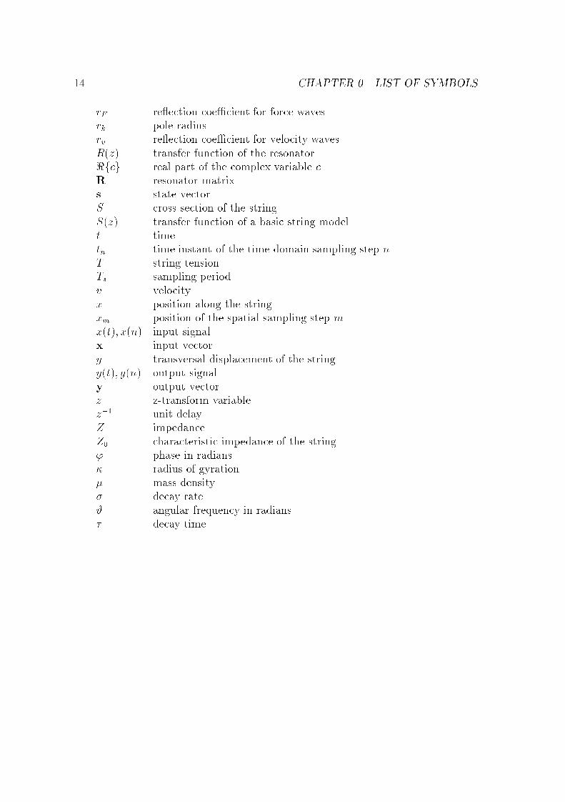
14 CHAPTER 0. LIST OF SYMBOLS

rF re�ection coe�cient for force wavesrk pole radiusrv re�ection coe�cient for velocity wavesR(z) transfer function of the resonator<fcg real part of the complex variable cR resonator matrixs state vectorS cross section of the stringS(z) transfer function of a basic string modelt timetn time instant of the time-domain sampling step nT string tensionTs sampling periodv velocityx position along the stringxm position of the spatial sampling step mx(t); x(n) input signalx input vectory transversal displacement of the stringy(t); y(n) output signaly output vectorz z-transform variablez�1 unit delayZ impedanceZ0 characteristic impedance of the string' phase in radians� radius of gyration� mass density� decay rate# angular frequency in radians� decay time

Chapter 1

Introduction

The aim of this thesis was understanding and simulating the sound generation of thepiano. Examining the physical principles of a musical instrument can be useful inmany ways: a better insight in the sound production mechanism of the piano couldlead to improvements of the instrument. On the other hand, it can be also appliedfor the design of sound synthesis algorithms, issuing in more realistic synthetic pianotones.

These two approaches yield di�erent modeling levels. While for understandingphysical phenomena complicated and accurate models are used, the e�cient soundsynthesis calls for simple and fast algorithms. Here we concentrate on the secondapproach. Accordingly, the proposed model captures only the most essential partsof the structure and sound generating behavior of the instrument.

The tasks for developing the structure of a physical model for an instrument arethe following: �rst, the acoustical properties of the instrument have to be carefullyinvestigated, then, a decision has to be made which features need to be simulated,the last step is �nding e�cient implementations for these features. After designingthe structure, the parameters of the model are calibrated. This is based on theanalysis of the real instrument. Thus, the design procedure both begins and endswith the analysis of the real world.

The physics-based approach has several advantages compared to traditionalmethods. The traditional techniques of sound synthesis simulate the resulting soundsignal by means of abstract algorithms or by the modi�cation of prerecorded sam-ples. Consequently, they hide the underlying sound production mechanism. More-over, their parameters have no meaning to the musician. This is similar to black-boxmodeling in system identi�cation. On the contrary, physical modeling techniquesconcentrate on the internal structure, similar to white-box models in the �eld ofsystem identi�cation. This way, the parameters of the model will have a more directinterpretation in the real word. They can be, e.g., the length of a string or the sti�-ness of the hammer felt. Once a speci�c instrument is designed, the modi�cation ofthe parameters will lead to meaningful results. For example, a modern grand pianocan be turned to an old pianoforte by changing two or three parameters. The largestbene�t of the physical modeling approach is that the interactions of the musician

15

16 CHAPTER 1. INTRODUCTION

are easily incorporated during sound synthesis.Nonetheless, physical modeling does not mean that all the parts of the model

have to be based on equations describing the behavior of the real piano. The gen-eral structure of the model originates from the real instrument, but some of theelements are modeled by non-physical algorithms. The aim is to incorporate themost advantageous methods for simulating the di�erent parts of the instrument.

The drawbacks of the physical modeling technique are the loss of generalityand the high implementation costs. While abstract algorithms or methods basedon prerecorded samples can be used for the reproduction of many kinds of instru-ments, a physical model is valid only for a speci�c instrument, or instrument family.Generally, physical models need more computational time compared to traditionaltechniques. Most likely these are the reasons why physical modeling techniques havenot gained signi�cance in the commercial synthesis market. Nevertheless, the yearby year increase in the computational power of digital signal processors can changethis state. Multimedia applications are also a promising �eld for the physics-basedmodeling of musical instruments.

Since this work deals with the physics-based modeling of the piano, the acousticalproperties of the instrument has to be discussed. This is done in Chapter 2, byreviewing the literature and presenting the results of own measurements. In Chapter3, di�erent sound synthesis algorithms are brie�y outlined, concentrating on theapplication to piano sound. Chapter 4 discusses the principles of digital waveguidemodeling, which is an e�cient technique for simulating the string behavior. Basedon the equations describing the digital waveguide, the equivalent resonator bankstructure is presented. In Chapter 5, we concentrate on the structure of the pianomodel. After presenting the general structure, the di�erent parts of the model arediscussed and several new methods are proposed. The model structure follows thatof the real piano. Namely, it consists of the hammer, string, and soundboard models.The chapter ends with the discussion of practical implementation issues. Chapter6 discusses the calibration of the di�erent parts presented in Chapter 5. Theseare aimed at determining the parameters of the model from measurements madeon real pianos. The goal is to �nd a parameter set to the model which gives themost similar sound output to the real piano. New calibration techniques are alsopresented. Finally, Chapter 7 summarizes the results and gives the planned directionof future research.

Chapter 2

Acoustical properties of the piano

The piano belongs to the group of struck string instruments. Historically, it is thedescendant of the harpsichord, but its excitation mechanism resembles that of theclavichord. The �rst piano was built as early as 1709 by Bartolomeo Cristofori, butit had to go through many changes to reach its modern form. This developmentwas mostly due to the work of Henry Steinweg in the middle of the 19th century.The comparison of a new and the 1720 Cristofori piano can be found in [Conklin1996a,b,c]. The upright pianoforte was developed in the middle of the nineteenthcentury [Fletcher and Rossing 1998]. Here we concentrate on the grand piano, butmost of the statements are valid for the upright piano as well. The description ofthe measurements can be found in the Appendix.

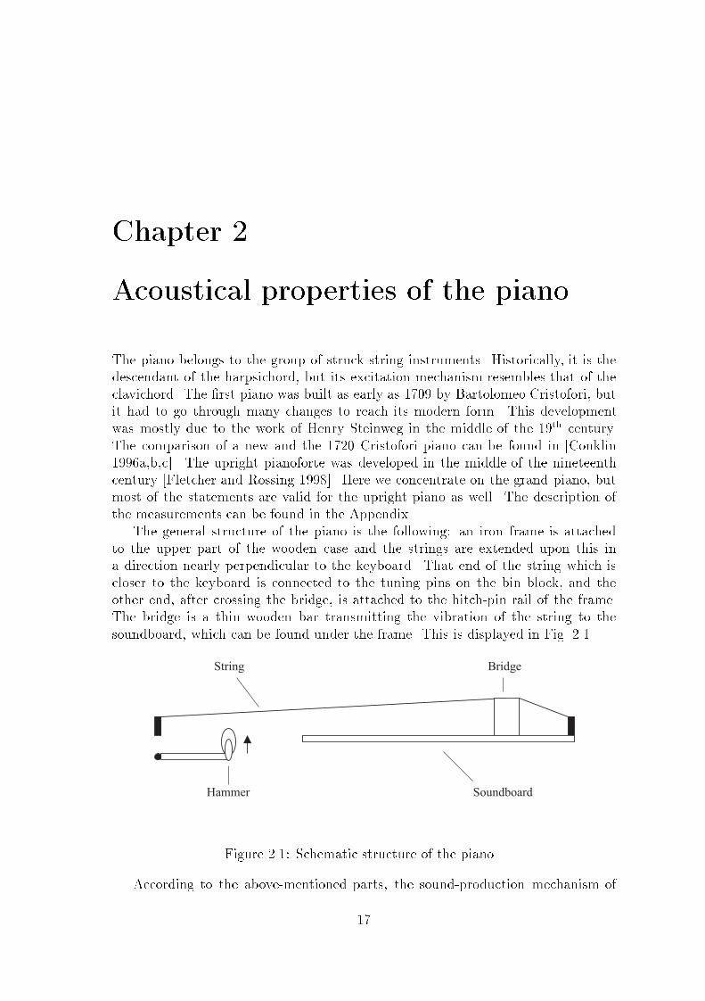
The general structure of the piano is the following: an iron frame is attachedto the upper part of the wooden case and the strings are extended upon this ina direction nearly perpendicular to the keyboard. That end of the string which iscloser to the keyboard is connected to the tuning pins on the bin block, and theother end, after crossing the bridge, is attached to the hitch-pin rail of the frame.The bridge is a thin wooden bar transmitting the vibration of the string to thesoundboard, which can be found under the frame. This is displayed in Fig. 2.1.

Figure 2.1: Schematic structure of the piano.

According to the above-mentioned parts, the sound-production mechanism of

17

18 CHAPTER 2. ACOUSTICAL PROPERTIES OF THE PIANO

the piano can be divided into the following steps:

1. The �rst is the excitation, the hammer strike. The piano action belongs to thispart as well, since it transmits the kinetic energy taken in by the artist to thekinetic energy of the hammer, which, after bouncing to the string, transformsto vibrational energy.

2. This energy is stored by the string in its normal modes. One part of that isdissipated due to internal losses, the other gets to the soundboard through thebridge.

3. The soundboard converts the vibrational energy to acoustical energy, to theaudible sound.

2.1 Piano action and hammer

2.1.1 The action

The action of the piano is an artwork of precision mechanics, and its operationis pretty complicated. This complexity is aimed at allowing the fastest possiblerepetition of a single note. In this way the repetition can be made before the hammerreaches its rest position. Roughly, the action can be considered as a lever systemwith a ratio of 1:5 between the movement of the key and the hammer. An important�avor of the action is that in the instant of hammer-string contact the hammerrotates freely. When the key is pressed down slowly, the hammer stops 4-6 mmbeneath the strings. Under normal playing conditions the hammer is sent towardsthe string by the transferred kinetic energy. By pressing a key the correspondingdamper is also lifted, which mutes the string by falling back after the key is released[Fletcher and Rossing 1998; Askenfelt and Jansson 1990, 1991].

By the examination of the timing of the action, Askenfelt and Jansson [1990]made some interesting observations. They concluded that the delay introduced bythe action depends on the dynamic level to a great extent. In the piano-legato touchthis delay can be as high as 100 ms, while at the forte-staccato touch from the hit ofthe key to the sound of the note elapses only 25 ms. Since this di�erence is audible,the skilled pianist must compensate for this actor. The key bottom contact canprovide some mechanical feedback to the player, since the di�erence there is in theorder of 15 ms, nevertheless skillful artists perform even more accurate timing.

The second article of the same series [Askenfelt and Jansson 1991] studies thedynamic properties of the action. There were contradicting standpoints betweenpianists and researchers concerning the possibilities of the pianist to in�uence thepiano tone. Researchers claimed that the resulting sound is controlled by the �-nal velocity of the hammer only. Nonetheless, pianists pay much attention to the�touch�. According to them considerable variations can be made in the tone thisway. Askenfelt and Jansson [1991] showed that the hammer exhibits various reso-nances and their level di�ers according to the type of touch. In legato playing, when

2.1. PIANO ACTION AND HAMMER 19

the action was accelerated continually, the amplitude of the hammer resonances wasconsiderably lower than that of the staccato touch. The resonant frequencies werefound at 50, 250 and 600 Hz with quality factor values between 15 and 30. It isstill unclear if these vibrations can have an in�uence on the string vibrations or not.Thus, it calls for future investigation.

2.1.2 The hammer

Hammers have a great in�uence on the timbre of the piano, since they excite thestrings. The hardwood cores of the hammers are covered by wool felt. The char-acteristics of the felt a�ect the resulting sound considerably. Harder felt results instronger partials, i.e., a brighter tone. On the contrary, softer hammers produceless partials and a softer tone. The timbre of the piano can be in�uenced by �voic-ing�. Hammers can be made softer by needling, or hardened by a hardening agent.Voicing is the last step of piano production, giving a �personality� to the instrument[Conklin 1996a].

The felt of the hammer is not homogeneous. Its hardness gradually changes fromthe outer part to the core. This is the main reason for the spectral di�erences atvarious dynamic levels: the high-frequency content of the tone increases with impactvelocity [Conklin 1996a; Askenfelt and Jansson 1993]. Consequently, the felt can beconsidered as a nonlinear spring, with a sti�ness increasing with compression. Anapproximate power-law model for the felt can be found in many articles [see, e.g.,Boutillon 1988]:

F = K(�y)p (2.1)

where �y refers to the compression of the felt, K is the sti�ness coe�cient and pis the sti�ness exponent. This may seem too simple for characterizing the complexbehavior of the hammer, but in practice, with proper K and p values, it describesthe hammer-string interaction at appropriate precision. These values (K and p)can be determined by curve-�tting from measured data [Boutillon 1988; Chaigneand Askenfelt 1994a]. Some papers suggest a hysteretic model for the hammer felt[Boutillon 1988; Stulov 1995]. An extensive theoretical and numerical analysis ofthe hammer-string interaction can be found in [Hall 1986, 1987a,b; Zhu and Mote1994].

The process of the hammer-string interaction is the following: the hammer,accelerated by the action, hits the string, but it does not bounce back immediately,since its mass is not negligible compared to the string. The hammer is thrownback by the re�ected pulses returning from the closer end of the string. The forceexperienced by the string (and the hammer) is a sequence of shock waves, whichgives to the graph of the force a lumpy character [Fletcher and Rossing 1998].

The shape and smoothness (and thus the frequency content) of the force curveis in�uenced by p, K and the initial velocity as well. Increasing K or the initialvelocity has the same e�ect, they both enlarge the high-frequency content of theexcitation. The average duration of the hammer-string contact is determined bythe ratio of the hammer and string mass. The heavier the hammer, the longer is

20 CHAPTER 2. ACOUSTICAL PROPERTIES OF THE PIANO

the contact time. With increasing initial velocities or K values the duration of thecontact decreases to some extent, but the signi�cance of this e�ect is much less thanthat of the mass ratio [Chaigne and Askenfelt 1994b; Fletcher and Rossing 1998].

The string is excited most e�ectively by the hammer when the contact time isequal to the half period of the tone. That's the case in the middle register. Onthe contrary, in the bass range the contact duration is much shorter, and in thetreble much longer than the ideal. In contemporary pianos, hammers of graduallychanging mass are used in order to reduce this e�ect [Conklin 1996a].

The spectra of the resulted sound depends on the striking point as well. Thisresults in a comb �ltering e�ect, since those modes of the string, which have a nodenear to the striking position cannot be excited e�ectively [Fletcher and Rossing1998; Conklin 1996a].

The model built for synthesis purposes (details are described later) allows theinvestigation of the hammer-string interaction. The results of the simulation werevery similar to those of the literature. The high-frequency content of the excitationforce increased with initial velocity and the contact time decreased by a negligibleamount. All other modi�cations on the excitation (hammer mass or sti�ness pa-rameter) gave the same results as those that can be found in the referred papers.This also justi�es the correctness of the model.

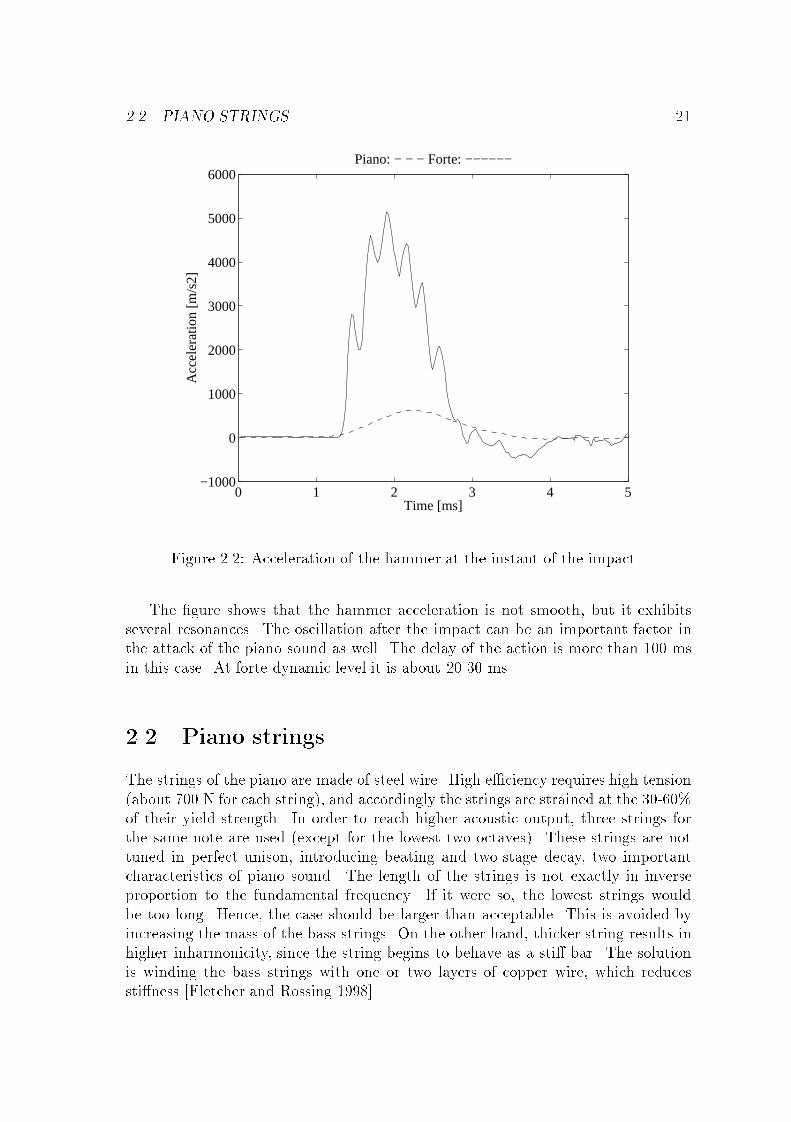
2.1.3 Measurement of the hammer behavior

The movement of the hammer was examined by a small accelerometer. In this waywe have an insight on the excitation signal, since one can estimate the shape of theforce experienced by the hammer from the acceleration of the hammer. The correctvalue of the force could be calculated only by knowing the inertia of the hammer.Consequently, the results shown here di�er from the force signal by a scaling factor.Ten di�erent keys were measured at various dynamic levels using legato and staccatotouch. The results resembled those found in the literature. Hammers in the middleregister showed resonances at about 20 and 300 Hz. These values are presumablylower than those of normal conditions, since adding the mass of the accelerometerlowers the frequency of the resonances. The measured contact times were similarto those of the referred papers. In Fig. 2.2 one can examine the acceleration ofthe hammer at the hammer-string contact at piano and forte levels (the measuredstring: A]

4, 467 Hz). For clarity the sign of the acceleration was inverted (since thehammer accelerates downwards during bouncing back from the string).

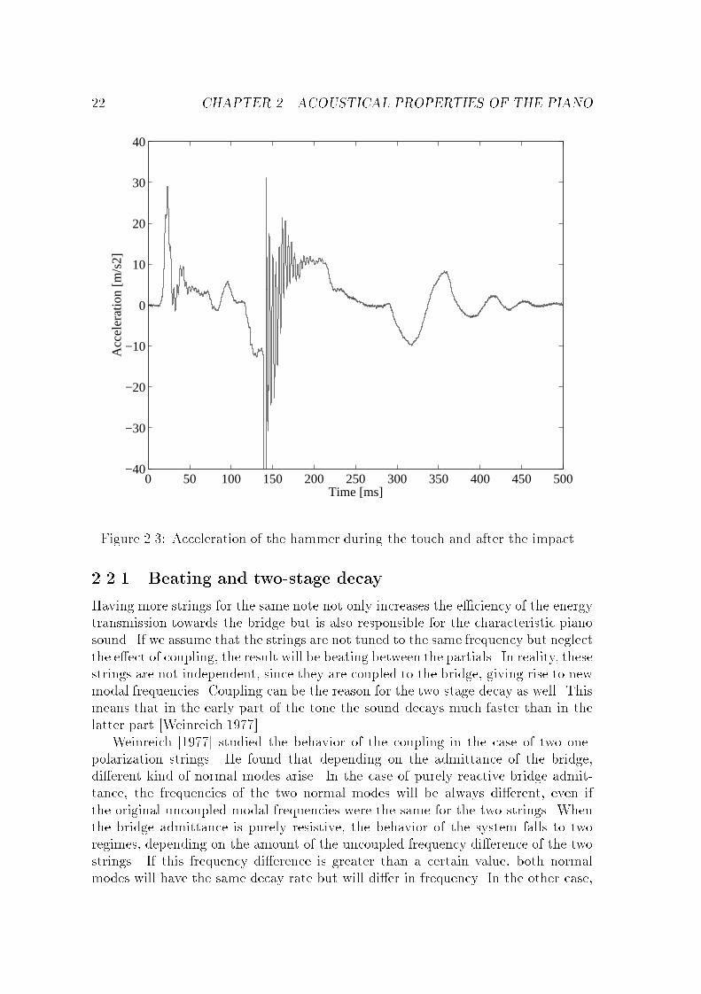
It can be seen that at higher initial velocities not only the amplitude of theexcitation force is changing but also its waveform. This is because of the nonlinearbehavior of the hammer felt. By vertically magnifying and horizontally compressingthe graph of the piano-level signal one can investigate the acceleration of the hammerbefore and after the impact (see Fig. 2.3). The �rst peak in the acceleration signalat around 20 ms corresponds to the beginning of the touch and the impact is nowrepresented by a vertical line at about 140 ms. Here positive values correspond toupward acceleration.

2.2. PIANO STRINGS 21

0 1 2 3 4 5−1000

0

1000

2000

3000

4000

5000

6000

Time [ms]

Acc

eler

atio

n [m

/s2]

Piano: − − − Forte: −−−−−−

Figure 2.2: Acceleration of the hammer at the instant of the impact.

The �gure shows that the hammer acceleration is not smooth, but it exhibitsseveral resonances. The oscillation after the impact can be an important factor inthe attack of the piano sound as well. The delay of the action is more than 100 msin this case. At forte dynamic level it is about 20-30 ms.

2.2 Piano strings

The strings of the piano are made of steel wire. High e�ciency requires high tension(about 700 N for each string), and accordingly the strings are strained at the 30-60%of their yield strength. In order to reach higher acoustic output, three strings forthe same note are used (except for the lowest two octaves). These strings are nottuned in perfect unison, introducing beating and two-stage decay, two importantcharacteristics of piano sound. The length of the strings is not exactly in inverseproportion to the fundamental frequency. If it were so, the lowest strings wouldbe too long. Hence, the case should be larger than acceptable. This is avoided byincreasing the mass of the bass strings. On the other hand, thicker string results inhigher inharmonicity, since the string begins to behave as a sti� bar. The solutionis winding the bass strings with one or two layers of copper wire, which reducessti�ness [Fletcher and Rossing 1998].

22 CHAPTER 2. ACOUSTICAL PROPERTIES OF THE PIANO

0 50 100 150 200 250 300 350 400 450 500−40

−30

−20

−10

0

10

20

30

40

Time [ms]

Acc

eler

atio

n [m

/s2]

Figure 2.3: Acceleration of the hammer during the touch and after the impact.

2.2.1 Beating and two-stage decay

Having more strings for the same note not only increases the e�ciency of the energytransmission towards the bridge but is also responsible for the characteristic pianosound. If we assume that the strings are not tuned to the same frequency but neglectthe e�ect of coupling, the result will be beating between the partials. In reality, thesestrings are not independent, since they are coupled to the bridge, giving rise to newmodal frequencies. Coupling can be the reason for the two-stage decay as well. Thismeans that in the early part of the tone the sound decays much faster than in thelatter part [Weinreich 1977].

Weinreich [1977] studied the behavior of the coupling in the case of two one-polarization strings. He found that depending on the admittance of the bridge,di�erent kind of normal modes arise. In the case of purely reactive bridge admit-tance, the frequencies of the two normal modes will be always di�erent, even ifthe original uncoupled modal frequencies were the same for the two strings. Whenthe bridge admittance is purely resistive, the behavior of the system falls to tworegimes, depending on the amount of the uncoupled frequency di�erence of the twostrings. If this frequency di�erence is greater than a certain value, both normalmodes will have the same decay rate but will di�er in frequency. In the other case,

2.2. PIANO STRINGS 23

the frequencies of the two normal modes will be the same, and their decay time willdi�er. If the admittance has both real and imaginary parts, as it is the case for areal soundboard, both the frequencies and decay times of the two normal modes candi�er. This means that the beating can grow and decay. The beating will reach itsmaximum when the amplitudes of the two modes approximately equal.

There is another explanation for the two-stage decay: the behavior of the twodi�erent polarizations. Since the vertical polarization of the string is coupled moree�ciently to the bridge than the horizontal polarization, the decay times di�ersigni�cantly. The hammer excites the vertical polarization to a greater extent, andthe energy transmission to the bridge is more e�ective in this direction as well. As aresult, in the beginning of the tone the sound produced by the vertical polarizationwill be the dominant. As the vibration of the vertical polarization decays faster, thelatter part of the tone will be determined by the horizontal polarization. However,these two polarizations are coupled to each other, so the description given here israther a simpli�cation of the real phenomenon. A detailed treatment on this subjectcan be found in [Weinreich 1977].

2.2.2 Inharmonicity

As mentioned earlier, the sti�ness of the strings results in a slightly inharmonicsound. The wave equation of the sti� string is the combination of the equations forthe ideal string (see Eq. 4.1) and ideal bar (for bending waves) [Morse 1948; Fletcherand Rossing 1998]:

�@2y

@t2= T

@2y

@x2�QS�2

@4y

@x4(2.2)

where x is the position along the string, y is the transversal string displacement,t is the time, T refers to tension and � to mass density. In Eq. (2.2) Q standsfor Young's modulus, S is the cross-section area of the string and � is the radius ofgyration. As a result of the forth-power term, dispersion will appear, and waves withhigher frequency will travel faster on the string, i.e., the wave velocity will not beconstant any more. The results of group velocity measurements in good agreementto the theory can be found in [Podlesak and Lee 1988]. As a result of dispersion,higher modes will go back and forth on the string within a shorter time, so theirfrequency will be somewhat higher than that of the ideal string. Solving Eq. (2.2)for small sti�ness the modal frequencies of the string will be the following [Fletcheret al. 1962; Fletcher and Rossing 1998; Morse 1948]:

fn = nf0p1 +Bn2 B =

�3Qd4

64l2T(2.3)

where f0 is the fundamental frequency of the ideal string, n is the number of thepartial, d is the diameter of the string and l is its length. The inharmonicity co-e�cient B can be calculated in this manner only for homogenous strings, but forwounded ones it is somewhat more di�cult, the precise formula gives a lower valuethan this. The exact formula can be found in [Fletcher and Rossing 1998]. It can

24 CHAPTER 2. ACOUSTICAL PROPERTIES OF THE PIANO

be seen from the equation that inharmonicity increases with partial number. TheB values are also increasing with the fundamental frequency of the string (since thelower strings are wound). On the contrary, when listening to piano sound, it seemsto be more inharmonic in the lower register than in the higher one. One reason forthis can be that the number of the partial which can be still heard is much higherfor the low strings. The other is a psychoacoustic phenomenon: for higher funda-mental frequencies the limit of perception for inharmonicity is higher than at lowfrequencies [Järveläinen et al. 1999]. The bandwidth of perceived inharmonicity wasstudied in [Rocchesso and Scalcon 1999].

It is an important question whether the inharmonicity is a desired factor orjust an unavoidable feature. Conklin [1996c] states that pianists usually choose thelargest piano available, which generally exhibits the lowest inharmonicity. The rea-son for this is that for low notes the amplitude of the fundamental is quite weak andthe determination of the pitch is mainly based on the higher partials. Due to inhar-monicity the frequency di�erence between partials is higher than the fundamentalfrequency and it increases with partial number. Accordingly, the de�nition of pitchbecomes uncertain. Conklin [1996c] concludes that inharmonicity is an importantfactor of piano sound, but there should be as little of it as possible.

Inharmonicity also a�ects piano-tuning. Since tuning is based on beating be-tween intervals (for �fths beating between the third partial of the lower note andthe second of the higher), stretching of partials will cause stretching of fundamentalfrequencies as well. As a result, the lowest notes of the piano are 30 cent below,while the highest are 30 cent above the tempered values. There appears to be apsychological reason for stretched tuning too, since listeners often judge intervalsas true octaves when their frequency ratio is slightly greater than 2:1 [Fletcher andRossing 1998].

2.2.3 Measurement of inharmonicity

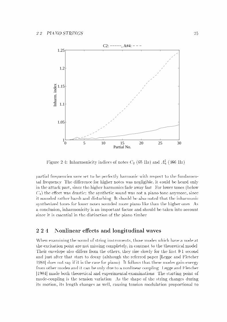
Several piano tones were recorded in this study with a microphone close to the sound-board. The results were similar to those of the literature. The graphs follow thetheoretical curves quite well. In Fig. 2.4 the inharmonicity indices (In = fn=(nf0))of the note C2 (65 Hz) and A]

4 (466 Hz) are plotted. The inharmonicity coe�cientscalculated by curve �tting were 0.0001 for C2 and 0.00075 for the A]

4 note. It can benoted that higher strings show higher inharmonicity, although perceptually they areconsidered to be less inharmonic. Besides the earlier mentioned reasons, anothercause for this di�erence can be that the higher partials of the higher note decaymuch faster than those of the lower one making the inharmonicity less audible.

Based on the measurements, subjective experiments were made in order to ex-plore whether it is needed or not to simulate inharmonicity in the synthesis model.Several piano tones were analyzed and resynthesized via additive synthesis. Thepartials had simple exponential decay curves �tted to measurements. The resultsounded like a somewhat unsuccessful attempt to synthesize piano tones, but it wasclear that it should be a piano sound. Then the dispersion was discarded, so all the

2.2. PIANO STRINGS 25

0 5 10 15 20 25 301

1.05

1.1

1.15

1.2

1.25C2: −−−−−, A#4: − − −

Partial No.

Inha

rm. i

ndex

Figure 2.4: Inharmonicity indices of notes C2 (65 Hz) and A]4 (466 Hz).

partial frequencies were set to be perfectly harmonic with respect to the fundamen-tal frequency. The di�erence for higher notes was negligible, it could be heard onlyin the attack part, since the higher harmonics fade away fast. For lower tones (belowC4) the e�ect was drastic: the synthetic sound was not a piano tone anymore, sinceit sounded rather harsh and disturbing. It should be also noted that the inharmonicsynthesized tones for lower notes sounded more piano-like than the higher ones. Asa conclusion, inharmonicity is an important factor and should be taken into accountsince it is essential in the distinction of the piano timbre.

2.2.4 Nonlinear e�ects and longitudinal waves

When examining the sound of string instruments, those modes which have a node atthe excitation point are not missing completely, in contrast to the theoretical model.Their envelope also di�ers from the others, they rise slowly for the �rst 0.1 secondand just after that start to decay (although the referred paper [Legge and Fletcher1984] does not say if it is the case for piano). It follows that these modes gain energyfrom other modes and it can be only due to a nonlinear coupling. Legge and Fletcher[1984] made both theoretical and experimental examinations. The starting-point ofmode-coupling is the tension variation. As the shape of the string changes duringits motion, its length changes as well, causing tension modulation proportional to

26 CHAPTER 2. ACOUSTICAL PROPERTIES OF THE PIANO

the elongation. By examining the lossy (�rst-order losses only), rigidly terminatedstring they concluded that the tension and the fundamental frequency decreaseexponentially as the sound decays. A modulation in tension at a double frequencyof the fundamental can be also found. In the case of completely rigid terminations,this tension variation can only a�ect the modes from which it originates. However,if one of the terminations has �nite impedance perpendicular to the string, modes nand m can transfer energy to the mode 2n �m. When the string passes the bridgeat an angle, the tension modulation exerts a force to the bridge perpendicular tothe strings. As the tension is modulated by twice the fundamental frequency, moden can deliver energy to the mode 2n [Legge and Fletcher 1984].

In a more recent paper [Hall and Clark 1987] claim that the nonlinear generationof missing modes is not the case for the piano, since the support is much more rigidthan that in Legge's and Fletcher's experiments. They explain that the small resid-ual amplitude of the �missing� modes comes from the �nite resistance of the bridge(they did not �nd the slow rise in the envelopes of these modes). The contradictionof the two papers has not been resolved yet, hence it calls for further research.

Conklin [1999] showed that the tension modulation is also audible in the acous-tical output of the piano. The so called �phantom partials� were only about 10 dBlower in amplitude than the nearest �real� partials. These were found at frequen-cies two times that of the exciting mode (2fn) and at sum and di�erence frequencies(fn�fm) of the exciting modes as well, contradicting the theoretical results of Leggeand Fletcher [1984]. The signi�cance of phantom partials is exceptionally high inthe case of piano, since they produce beating with the inharmonic real partials.Note that in a perfectly harmonic string the e�ect would be only a change in theinitial amplitude. This can be one of the reasons why pianists prefer pianos with lessinharmonicity, since in that case the frequency di�erence between real and phantompartials is lower.

The tension modulation as nonlinear coupling can also transfer energy betweenthe two transversal polarizations. As a result, the polarization ellipse does not re-main still but it features a slow precession [Fletcher and Rossing 1998] Experimentalresults on the subject can be found in [Hanson et al. 1994].

According to Giordano and Korty [1994], tension modulation is the cause of therise of longitudinal waves as well. Their starting-point was the observation that themusical sound is preceded by a precursor signal. This precursor has to be transferredby the longitudinal waves since they travel faster than the transversal ones. Theyare excited by the tension-variation exerted by the hammer strike.

The relative frequencies of the longitudinal modes also in�uence the quality ofthe piano sound. The di�erence between the �rst transversal and longitudinal modesis typically between 4200 and 5200 cents (42-52 semitones), and it is constant ir-respectively of the tuning of the string. In order to reach good quality, the �rstlongitudinal mode should be in tune with the piano. This means that it shouldcoincide with the �rst transversal mode of any higher note [Conklin 1996c].

2.3. THE BRIDGE AND THE SOUNDBOARD 27

2.3 The bridge and the soundboard

The soundboard of modern pianos is generally made of assembling strips of solidsoftwood (such as Sitka or red spruce). These 5-15 cm wide strips are glued together.Since the sti�ness of the wood is higher along the grain, the cross-grain sti�ness isincreased by adding ribs to the soundboard. This increases the travel velocity inthat direction. Pianos of lower cost are generally built of laminated wood. Thecomparison of soundboards of di�erent materials can be found in [Conklin 1996b].

The vibration of the strings is transmitted to the soundboard through the bridge.The bridge functions as an impedance transformer, presenting higher impedance tothe string than that if the strings were directly connected to the soundboard. In thelatter case decay times would be too short. By carefully designing the soundboardand the bridge the loudness and the decay time of the partials can be set, althoughthese parameters are in an inverse ratio [Fletcher and Rossing 1998].

The impedance curve of the soundboard exhibits a high modal density. Manystudies have been done on the low frequency behavior of the soundboard. Theseresonances are similar to the simple motion of a plate and can be easily observed bythe Chladni method [Conklin 1996b]. The higher frequency region of the soundboardwas investigated by Giordano [1998]. He found that the average of the impedance isconstant up to about 3-7 kHz (between 1000 and 10000 kg/s) and after that it startsto decrease with frequency. This decline is due to the ribs. Although the sti�ness ofthe soundboard di�ers in the di�erent directions, without ribs it would not producethis result, since the modal density would remain constant. According to Giordano[1998] the ribs sti�en the soundboard at lower frequencies to a higher extent, as athigher frequencies the modes �t in between the ribs. This result was supported bynumerical simulations as well [Giordano 1997].

2.3.1 Measurement of the soundboard

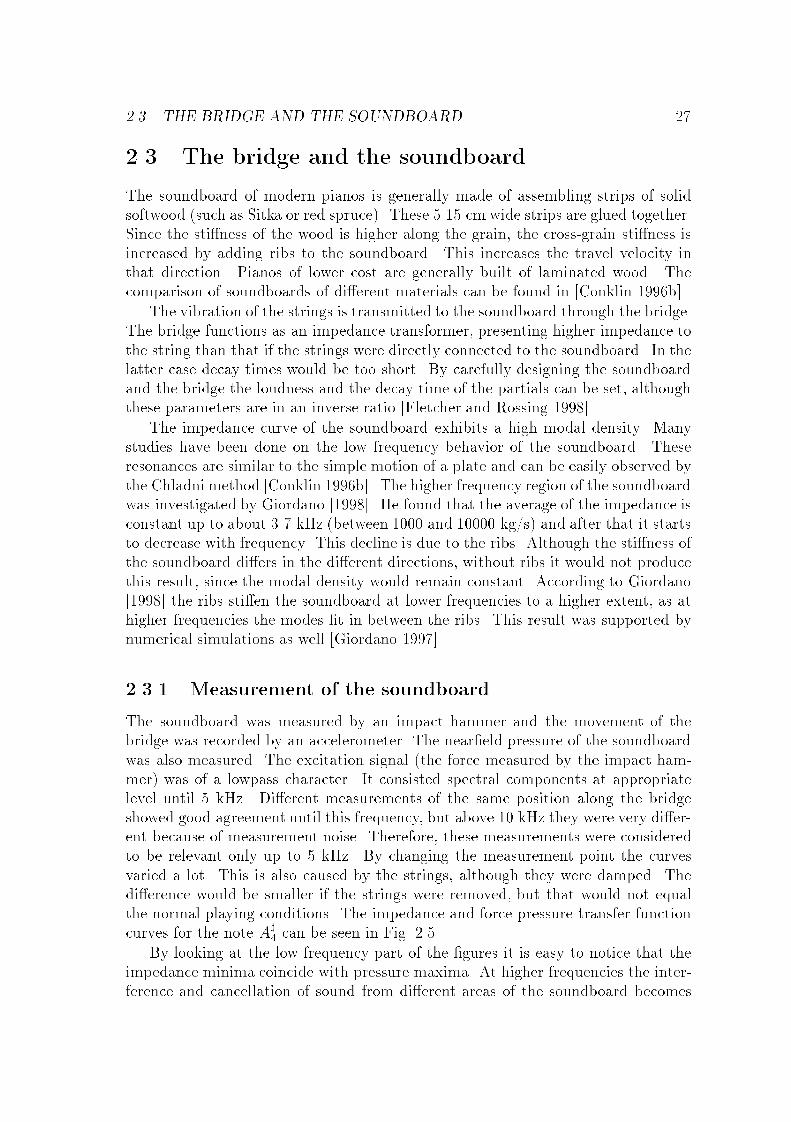
The soundboard was measured by an impact hammer and the movement of thebridge was recorded by an accelerometer. The near�eld pressure of the soundboardwas also measured. The excitation signal (the force measured by the impact ham-mer) was of a lowpass character. It consisted spectral components at appropriatelevel until 5 kHz. Di�erent measurements of the same position along the bridgeshowed good agreement until this frequency, but above 10 kHz they were very di�er-ent because of measurement noise. Therefore, these measurements were consideredto be relevant only up to 5 kHz. By changing the measurement point the curvesvaried a lot. This is also caused by the strings, although they were damped. Thedi�erence would be smaller if the strings were removed, but that would not equalthe normal playing conditions. The impedance and force-pressure transfer functioncurves for the note A]

4 can be seen in Fig. 2.5.

By looking at the low-frequency part of the �gures it is easy to notice that theimpedance minima coincide with pressure maxima. At higher frequencies the inter-ference and cancellation of sound from di�erent areas of the soundboard becomes

28 CHAPTER 2. ACOUSTICAL PROPERTIES OF THE PIANO

102

103

102

103

104

Impe

dane

[kg/

s]

Frequency [Hz]

102

103

−40

−30

−20

−10

0

P/F

[dB

]

Frequency [Hz]

Figure 2.5: Impedance and force-pressure transfer function of the soundboard.

more signi�cant, and the former coincidence cannot be found any longer. The aver-age value of the soundboard impedance is similar to the results of Giordano [1998],although the decrease with frequency cannot be observed. To answer this question,new measurements are needed which can be used at least up to 10 kHz.

2.4 Pedals

Pianos have either two or three pedals. The most important one is the sustain pedalon the right, which lifts the dampers of all the strings. This sustains the struck keyson the one hand and also changes the character of the timbre on the other, since allthe other strings can vibrate freely in sympathetic mode.

The e�ect of the sustain pedal was also measured. The bridge was hit by animpact hammer and the acceleration of the bridge and the near-�eld sound pressurewere recorded. The impedance curve of the bridge did not change signi�cantlycompared to that without sustain pedal. The resonances became more peaky but thedi�erence of the two curves stayed below one or two decibels. The main reason for thetimbral change is not the change of the impedance but of the force-pressure transfer

2.5. SPECTRA OF THE PIANO SOUND 29

function. The 300-400 ms long attack noise coming from the impulse response of thesoundboard remains the same but it is superimposed on the slow (10-20 sec long)decay of string vibrations. The impulse response varies largely with the measurementposition: hitting the bridge at the low register results in a softer timbre, hitting atthe high stings in a brighter one.

The left pedal is the una corda pedal, which shifts the entire action sideways.Consequently, the hammers strike only two strings out of three in the treble, orone out of two in the midrange. This causes only about 1 dB reduction of thesound pressure level, but changes the timbre [Fletcher and Rossing 1998]. One ofthe reasons for this is that the third string gains energy from the vibration of theother two. The initial conditions of the coupled vibration are changed, resulting ina slower decay [Weinreich 1977]. Another reason for the spectral change can be thatwhen the same hammer hits a smaller number of strings, it appears to be heavierwith respect to the single strings, causing longer contact times and a softer timbre.

In upright pianos, the left pedal is a soft pedal. It moves the hammers closer tothe string, resulting in lower striking force [Fletcher and Rossing 1998].

The middle pedal is the sustenuto pedal, which sustains only those notes thathave been hit before depressing the pedal. In some uprights, this is a practice pedal,which lowers a piece of felt between the strings and the hammers [Fletcher andRossing 1998].

2.5 Spectra of the piano sound

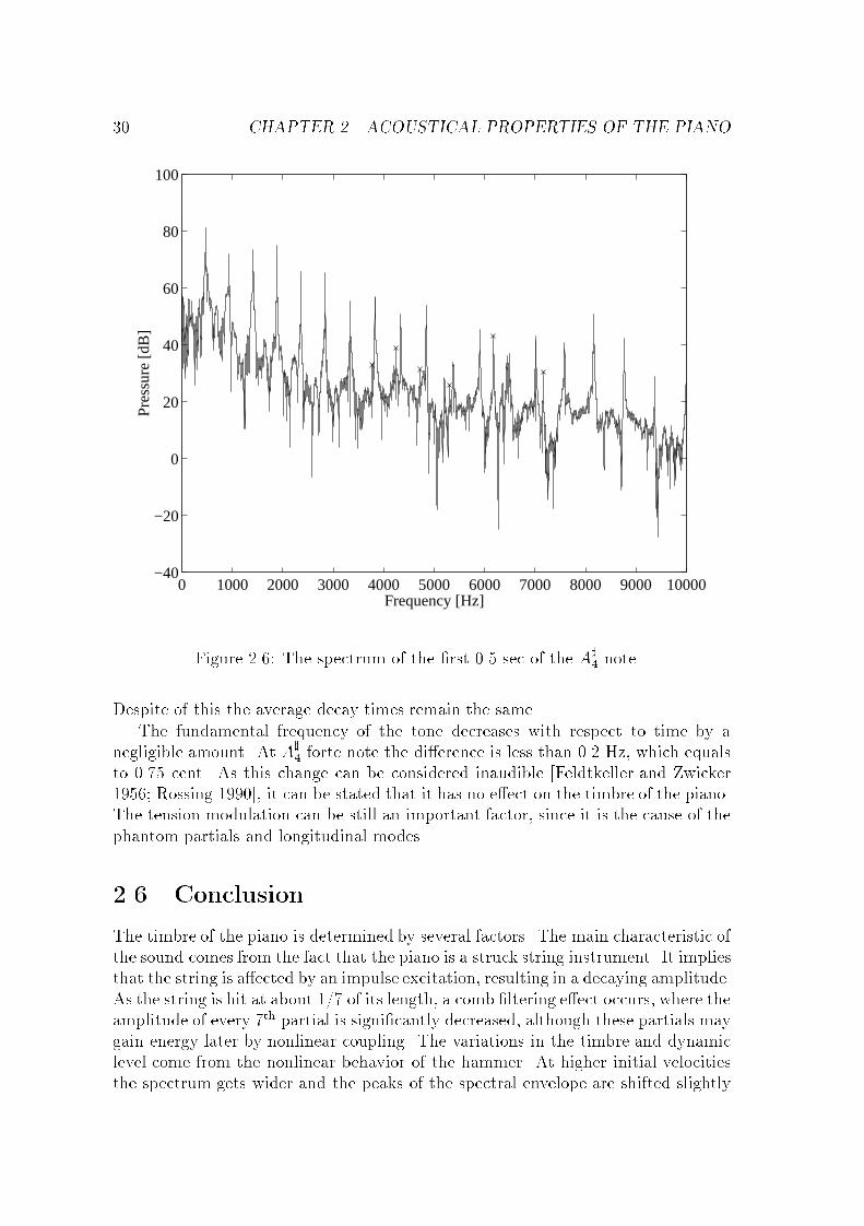
Fig. 2.6 shows the spectrum of the �rst 0.5 sec of the A]4 note at forte dynamic level.

The inharmonicity can be easily recognized: the distance between partials gets largeras the frequency increases. Between the real partials the phantom partials can alsobe found. Some are marked by � in Fig. 2.6. The frequencies of the marked phantompartials in terms of the real partial frequencies are: 2f4, f4+f5, 2f5, f1+f10, f6+f7,and f7 + f8.

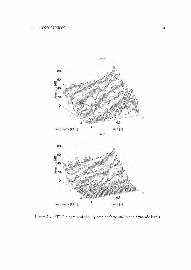
The upper part of Fig. 2.7 illustrates the STFT (Short Time Fourier Transform)of the �rst second of the same note up to 5 kHz. The length of the Hammingwindow was four times the pitch period. The envelopes of the distinct partialsevolve di�erently as a result of the complex coupling. The basic phenomenon is thebeating whose frequency is proportional to the partial number. The two-stage decayis not visible, since the displayed 1 sec time is too short for that.

The lower part of Fig. 2.7 shows the STFT diagram of the same note at pianolevel. It can be seen that not only the overall amplitude but also the level ratio ofthe partials changes. At lower hammer velocities the spectrum decays more steeplywith frequency. The time-domain evolutions of the envelopes exhibit di�erences aswell. The reason for this can be the nonlinear string behavior on one hand and thedi�erent excitation of the individual strings on the other. Because of the unevennessof the felt the hammer compliance for the distinct strings can be dissimilar, so thestrings gain energy from the hammer with di�erent ratios at di�erent dynamic levels.

30 CHAPTER 2. ACOUSTICAL PROPERTIES OF THE PIANO

0 1000 2000 3000 4000 5000 6000 7000 8000 9000 10000−40

−20

0

20

40

60

80

100

Frequency [Hz]

Pre

ssur

e [d

B]

Figure 2.6: The spectrum of the �rst 0.5 sec of the A]4 note.

Despite of this the average decay times remain the same.The fundamental frequency of the tone decreases with respect to time by a

negligible amount. At A]4 forte note the di�erence is less than 0.2 Hz, which equals

to 0.75 cent. As this change can be considered inaudible [Feldtkeller and Zwicker1956; Rossing 1990], it can be stated that it has no e�ect on the timbre of the piano.The tension modulation can be still an important factor, since it is the cause of thephantom partials and longitudinal modes.

2.6 Conclusion

The timbre of the piano is determined by several factors. The main characteristic ofthe sound comes from the fact that the piano is a struck string instrument. It impliesthat the string is a�ected by an impulse excitation, resulting in a decaying amplitude.As the string is hit at about 1/7 of its length, a comb �ltering e�ect occurs, where theamplitude of every 7th partial is signi�cantly decreased, although these partials maygain energy later by nonlinear coupling. The variations in the timbre and dynamiclevel come from the nonlinear behavior of the hammer. At higher initial velocitiesthe spectrum gets wider and the peaks of the spectral envelope are shifted slightly

2.6. CONCLUSION 31

00.5

1

0

2

4

0

20

40

60

80

Time [s]

Forte

Frequency [kHz]

Pre

ssur

e [d

B]

00.5

1

0

2

4

0

20

40

60

80

Time [s]

Piano

Frequency [kHz]

Pre

ssur

e [d

B]

Figure 2.7: STFT diagram of the A]4 note at forte and piano dynamic levels.

32 CHAPTER 2. ACOUSTICAL PROPERTIES OF THE PIANO

to the right.The kinetic energy of the hammer transforms to the vibrational energy of the

string. The main part of this energy is stored by the string, the second slowly getsto the soundboard and the third part dissipates. The string determines the funda-mental frequency of the note and in�uences the decay of the partials. The decay andthe transmitted energy also depend on the terminating impedance. At impedancemaxima of the soundboard the partials can deliver less energy to the soundboardduring the same amount of time. Therefore, their amplitudes will be lower andtheir decay times longer than those which are located at impedance minima. Thesti�ness of the string results in a high dispersion. There is no other western stringinstrument where the inharmonicity would be as high as in the case of the piano.Simulation results and informal listening experiments show that inharmonicity isespecially important at the low register of the piano.

The di�erent coupling of the two polarizations to the soundboard results in atwo-stage decay. The envelope of the partials decays faster in the early part of thetone than in the latter. The slight frequency di�erence of the two or three stringscauses beating. The resulting amplitude modulation is quite complicated becauseof the coupling of the strings. The tension modulation gives rise to longitudinalwaves whose relative amplitude to the transversal modes increases with dynamiclevel. The appearance of phantom partials comes from the tension modulation aswell. The three strings and their three di�erent polarizations constitute a complexnonlinearly coupled system, issuing in a dynamic change of the timbre.

The soundboard, besides in�uencing the decay times, determines the overallspectrum signi�cantly. Its behavior can be assumed to be linear, but its numerousresonances alter the timbre largely. The characteristic attack noise of the pianosound comes mainly from the impulse response of the soundboard, but also fromthe noise of the action.

Chapter 3

Overview of synthesis methods

Here we brie�y overview the di�erent techniques used for sound synthesis purposes,and their application to the piano. The details of the algorithms will not be given, formore thorough discussion see [Roads 1995; Tolonen et al. 1998]. The classi�cationof di�erent methods is based on the work of Smith [1991] and Tolonen et al. [1998].

3.1 Abstract algorithms

Here we discuss abstract algorithms. Their advantages are simplicity, generality, andthe small number of control parameters. The drawback is that analysis proceduresare complicated, making it almost impossible to simulate the sound of many realinstruments. They are rather useful for creating synthetic, never heard sonorities.

The FM (frequency modulation) synthesis was presented by [Chowning 1973].It is founded from the theory of frequency modulation used in radio transmission,but the frequencies of the modulating and carrier waves are in the same order here.Its advantage is that even a two-oscillator system can produce a rich spectrum.Inharmonic sounds can also be generated by this technique. If both the carrier andmodulating waves are sinusoids, the amplitudes of the resulting harmonics can becalculated by the Bessel functions. Van Duyne [1992] used the FM synthesis formodeling inharmonic low piano tones.

The waveshaping synthesis was developed by Le Brun [1979] and Ar�b [1979]. Itis based on the nonlinear distortion of a simple input signal. An advantage is that theamplitude variation of the signal results in a large alteration of the output spectrum.When the input signal is sinusoidal, the amplitudes of the resulting harmonics aredetermined by the Chebyshev polynomials. This way, the shaping function can beanalytically derived from the partial amplitudes. The method is capable to simulateharmonic spectra only.

The Karplus-Strong algorithm [Karplus and Strong 1983] is a simple algorithmbased on the modi�cation of the wavetable synthesis. In the wavetable synthesis,the signal is periodically read from a computer memory. In the Karplus-Strongalgorithm the sample is modi�ed after reading and written back to the same position.This way, the content of the wavetable will evolve with time. The algorithm has

33

34 CHAPTER 3. OVERVIEW OF SYNTHESIS METHODS

been found very e�cient in the simulation of plucked string and drum timbres.However, it was found soon that the Karplus-Strong algorithm is a special case ofthe technique now called digital waveguide modeling [Ja�e and Smith 1983; Smith1983].

3.2 Processing of pre-recorded samples

The methods described here are based on recording and processing of real sounds.Accordingly, they are very accurate in reproducing the speci�c sound, which wasrecorded. They are not able to reproduce the changes in playing conditions, i.e., thesimulation of not recorded sounds is not realistic. Another problem is that a largeamount of data is needed for describing the instruments.

Sampling synthesis is the basic form of these algorithms. All the commerciallyavailable digital pianos use this technique. They store separate tones of the instru-ment in a memory and play it back when a key is depressed [Roads 1995]. Thememory need is reduced by looping, that is, continuously repeating the steady statepart of the tone. The amplitude and timbre evolution of the piano is simulated by atime-varying amplitude envelope and a time-varying �lter. Di�erent dynamic levelsare taken into account by modifying these envelopes, hence a forte note results ina brighter and louder sound than a piano one. The method synthesizes the notesseparately. Therefore, it cannot simulate the coupled vibrations of the strings or therestrike of the same string. Nevertheless, even if physical models theoretically couldprovide better results, the highest quality synthesized piano sounds are coming fromdevices using the sampling technique. Also an advantage is that the implementationof the algorithm is simple. Sampling synthesis can be successful in the synthesis ofpiano sound, because the impact velocity can be easily mapped to the amplitudeand �lter envelopes. Other instruments, such as the violin, where the musician hasmore in�uence on the sound, could not be realistically simulated.

Multiple wavetable synthesis is in a way similar to sampling synthesis. One mu-sical tone is reproduced by many wavetables, whose content is interpolated [Roads1995]. It also resembles additive synthesis since the wavetables have separate ampli-tude envelopes and their output is summed. In [Yuen and Horner 1997] the attackof sounds were synthesised by sampling, and for the decay part multiple wavetablesynthesis was used.

Granular synthesis is based on composing the synthetic sounds from short soundelements in the time domain [Roads 1995]. The algorithms can be divided intoasynchronous and pitch synchronous methods. The �rst method can rahter be usedfor creating synthetic sounds. For the reproduction of musical instrument sounds,usually the latter one is applied.

3.3. SPECTRAL MODELS 35

3.3 Spectral models

Spectral models try to approach the synthesis problem from the spectral domain,which is more similar to the human sound perception. Some of them also takepsychoacoustic criteria into account. Their advantage comes from this fact. Adrawback is that generally many parameters are needed for the description of aninstrument. The simulation of transients is problematic, which makes them di�cultto use for the synthesis of piano sound.

The simplest spectral technique is the additive synthesis. It is based on summingsinusoidal signals with di�erent frequency and amplitude envelopes. It is popularsince its mathematical background, the Fourier transform, is well developed. Anadvantage of the additive technique is the �exibility. Its drawback is the hugenumber of control parameters. [Fletcher et al. 1962] used this technique for thesynthesis of piano sound by means of analog circuits.

Group additive synthesis is a combination of additive and wavetable synthesistechniques. It is motivated by the need for reducing the control stream of theadditive synthesis. Therefore, some partials are grouped together and they willhave common frequency and amplitude envelopes. These grouped partials are thencombined to form wavetables. Lee and Horner [1999] used the method for modelingthe sound of the piano. The grouping of the partials was determined with the helpof genetic algorithms. In Zheng [1999], a critical-band based grouping was used.

Spectral modeling synthesis is a method which decomposes the sound into deter-ministic and stochastic components in the spectral domain [Serra and Smith 1990].More recently, methods for deterministic, stochastic and transient decompositionwere developed [Verma and Meng 1995]. Modeling the transients seems to be essen-tial in synthesizing piano sound.

3.4 Physical modeling

The main feature of physical modeling approaches is that they model the originof the sound phenomenon, and not the resulting signal. This issues in a realisticresponse to the interactions of the musician, since the input parameters of the modelare analogous with the real world. Theoretically, the physical modeling approachcould give the most realistic synthetic instrument sounds. Their drawback is the lossof generality and the high computational cost. The calibration of the parameters isnot always trivial either.

The �rst method used in physical modeling was the discrete time solution of the�nite di�erence equation [Hiller and Ruiz 1971a,b]. The �nite di�erence method wasapplied for simulating the string of the piano in [Chaigne and Askenfelt 1994a,b].Giordano [1997] used the technique for modeling the soundboard of the piano. Acomplete piano model based on the �nite di�erence method was presented in [Hikichiand Osaka 1999]. The advantage of the approach is that the physical equations canbe directly implemented as algorithms. Its drawback is the high computational cost,

36 CHAPTER 3. OVERVIEW OF SYNTHESIS METHODS

especially if the structure is not one-dimensional.Modal synthesis describes the structure with the linear combination of vibration

modes [Adrien 1991]. Its main advantage is the generality, since the same kind offormulation can be used for the simulation of every vibrating structure. Analy-sis techniques for the determination of the modal parameters are already available,mostly used in the car and aircraft industry. However, these tools are rather expen-sive for academic research. The parameters of the model have physical meanings,but they are not intuitive. The visible parameters of the real structure, e.g., thelength of the string, are hidden.

The exciter-resonator technique was used in [Laroche and Meillier 1994] for thesynthesis of piano sound. A common excitation signal was derived which was �lteredthrough the resonators. The drawback of the exciter-resonator approach is that itis not capable of simulating nonlinear interaction.

McIntyre et al. [1983] recognized that most of the instruments can be simulatedwith a nonlinearity and a linear element in a feedback loop. The linear element isthe re�ection function, whose main feature is the delay.

Smith [1983, 1987, 1992] proposed a computationally very e�cient technique,the digital waveguide modeling. The method is based on the discretization of thetime-domain solution of the wave equation. The e�ciency of the digital waveguidelies in lumping the losses and dispersion of the structure to one point. Hence, thestring or acoustic tube is simulated by a delay and a linear �lter. In this way, it issimilar to the approach of McIntyre et al. [1983]. The Karplus-Strong algorithm isa special case of digital waveguide modeling [Ja�e and Smith 1983]. The �rst pianomodel based on the digital waveguide was presented in [Garnett 1987]. There, thedigital waveguides were connected to a common termination. In [Borin et al. 1997]a nonlinear hammer model was used. The computationally most e�cient digitalwaveguide piano model is the commuted piano proposed in [Smith and Van Duyne1995; Van Duyne and Smith 1995]. Since these are the approaches, which are mostsimilar to the model presented in this thesis, their detailed description will be givenin Chapter 5 with relation to the proposed model structure.

3.5 Conclusion

Until this time, the sampling synthesis has given the best results in synthesizing thepiano tone. If all the notes of the piano are recorded at di�erent dynamic levels,no other synthesis method can result in more realistic sound. The author believesthat the only exception is the physical modeling, since it can take into account theinteraction of the di�erent parts, such as the coupling between di�erent strings. Thesingle weak point of sampling synthesis is that it treats the sounds separately. Theonly way to make a better synthesis method is to attack this weakness. However, thephysical model described in this thesis does not completely ful�ll this requirementyet. It can be only considered as a �rst step towards the high quality synthesis ofpiano sound.

Chapter 4

Principles of string modeling

In this chapter the mathematical background of digital waveguide modeling is pre-sented. The formulation originates from the time-domain solution of the wave equa-tion. After an overview of the ideal string, the e�ect of losses and dispersion isdiscussed. This chapter also introduces a new resonator bank interpretation andshows its equivalence to the digital waveguide model.

4.1 Modeling the ideal string

An e�ective approach for modeling a string and an acoustical tube was introducedby Smith [1987, 1992]. The method is based on the discretization of the time-domainsolution of the wave equation.

By forming the wave equation of the ideal string, it is needed to make severalsimpli�cations: the length of the string is assumed to be in�nite, its mass density� and tension T is supposed to be homogenous and its displacement to be smallwith respect to string length, which means that its slope is very small (dy=dx� 1).Furthermore, only one transversal polarization of the string is taken into account.The result is the one-dimensional wave equation Eq. (4.1), which is similar to that oftransmission lines or the longitudinal motion of bars. The derivation of this equationcan be found in the literature [Morse 1948; Fletcher and Rossing 1998] et al.

@2y

@x2=

1

c2@2y

@t2; c =

sT

�(4.1)

In Eq. (4.1) x is the position along the string, y is the transversal displacement,t stands for time, T for the tension, � for linear mass density and c for the wavevelocity. The equation shows that the acceleration of a small section of the stringis proportional to the curvature of the string at that section. Every traveling wavewhich retains its shape is a solution of the wave equation. Because of the linearityof the string, the general solution is a superposition of two traveling waves; one ofthem going to the right, the other to the left direction:

y(x; t) = f+(ct� x) + f�(ct+ x)

37

38 CHAPTER 4. PRINCIPLES OF STRING MODELING

v(x; t) =dy

dt= c

df+

dt(ct� x) + c

df�

dt(ct+ x) (4.2)

According to these equations, the shapes of the two traveling-waves f+ and f� arecompletely determined by the initial displacement y(x; 0) and velocity v(x; 0).

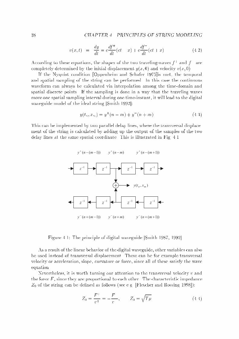
If the Nyquist condition [Oppenheim and Schafer 1975]is met, the temporaland spatial sampling of the string can be performed. In this case the continuouswaveform can always be calculated via interpolation among the time-domain andspatial discrete points. If the sampling is done in a way that the traveling wavesmove one spatial sampling interval during one time-instant, it will lead to the digitalwaveguide model of the ideal string [Smith 1992]:

y(tn; xm) = y+(n�m) + y�(n+m) (4.3)

This can be implemented by two parallel delay lines, where the transversal displace-ment of the string is calculated by adding up the output of the samples of the twodelay lines at the same spatial coordinate. This is illustrated in Fig. 4.1.

Figure 4.1: The principle of digital waveguide [Smith 1987, 1992].

As a result of the linear behavior of the digital waveguide, other variables can alsobe used instead of transversal displacement. These can be for example transversalvelocity or acceleration, slope, curvature or force, since all of these satisfy the waveequation.

Nevertheless, it is worth turning our attention to the transversal velocity v andthe force F , since they are proportional to each other. The characteristic impedanceZ0 of the string can be de�ned as follows (see e.g. [Fletcher and Rossing 1998]):

Z0 =F+

v+= �F

�

v�; Z0 =

qT� (4.4)

4.1. MODELING THE IDEAL STRING 39

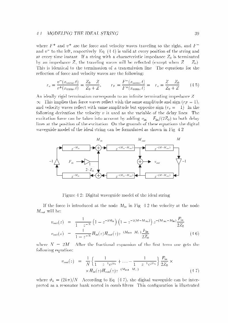
where F+ and v+ are the force and velocity waves traveling to the right, and F�

and v� to the left, respectively. Eq. (4.4) is valid at every position of the string andat every time instant. If a string with a characteristic impedance Z0 is terminatedby an impedance Z, the traveling waves will be re�ected (except when Z = Z0).This is identical to the termination of a transmission line. The equations for there�ection of force and velocity waves are the following:

rv =v�(xterm; t)

v+(xterm; t)=Z0 � Z

Z0 + Z; rF =

F�(xterm; t)

F+(xterm; t)= �rv = Z � Z0

Z0 + Z(4.5)

An ideally rigid termination corresponds to an in�nite terminating impedance Z =1. This implies that force waves re�ect with the same amplitude and sign (rF = 1),and velocity waves re�ect with same amplitude but opposite sign (rv = �1). In thefollowing derivation the velocity v is used as the variable of the delay lines. Theexcitation force can be taken into account by adding vin = Fin=(2Z0) to both delaylines at the position of the excitation. On the grounds of these equations the digitalwaveguide model of the ideal string can be formulated as shown in Fig. 4.2.

Figure 4.2: Digital waveguide model of the ideal string.

If the force is introduced at the node Min in Fig. 4.2 the velocity at the nodeMout will be:

vout(z) =1

1 � z�N

�1� z�2Min

� �1� z�2(M�Mout)

�z�(Mout�Min)

Fin

2Z0

vout(z) =1

1 � z�NHin(z)Hout(z)z

�(Mout�Min)Fin

2Z0(4.6)

where N = 2M . After the fractional expansion of the �rst term one gets thefollowing equation:

vout(z) =1

N

�1

1� z�1ej#1+ : : :+

1

1 � z�1ej#N

�Fin

2Z0�

�Hin(z)Hout(z)z�(Mout�Min) (4.7)

where #k = (2k�)=N . According to Eq. (4.7), the digital waveguide can be inter-preted as a resonator bank nested in comb �lters. This con�guration is illustrated

40 CHAPTER 4. PRINCIPLES OF STRING MODELING

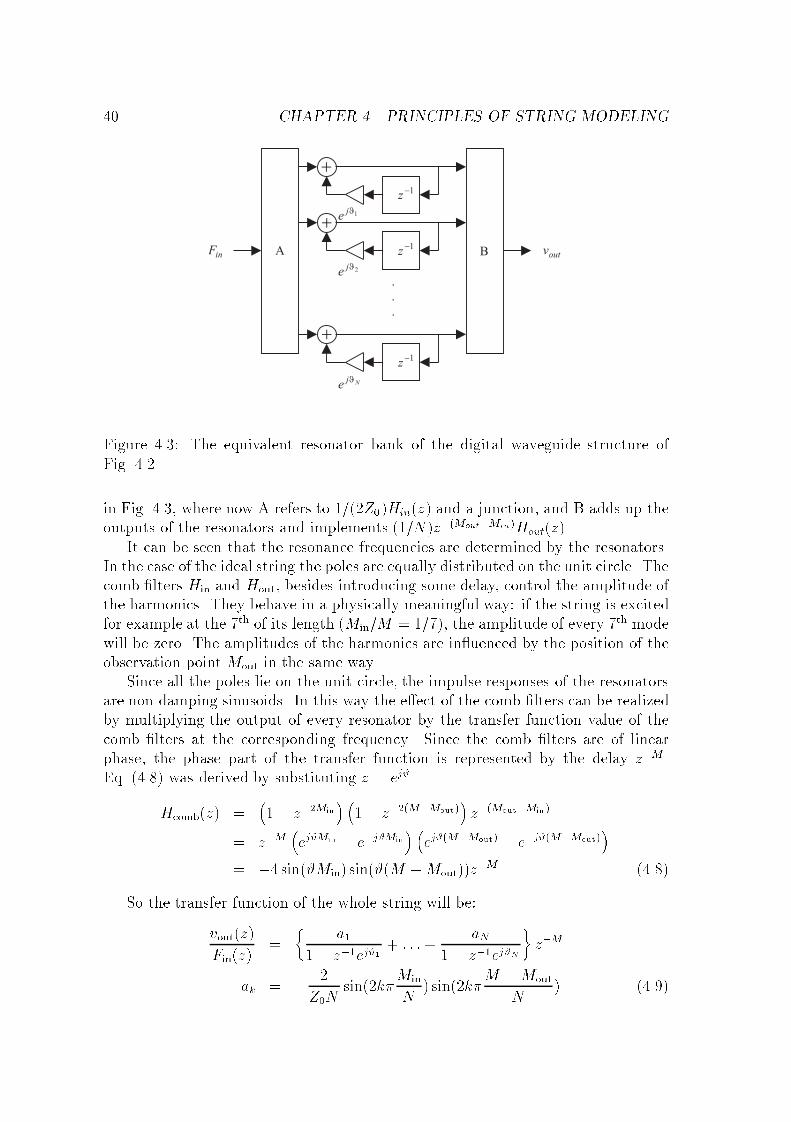
Figure 4.3: The equivalent resonator bank of the digital waveguide structure ofFig. 4.2.

in Fig. 4.3, where now A refers to 1=(2Z0)Hin(z) and a junction, and B adds up theoutputs of the resonators and implements (1=N)z�(Mout�Min)Hout(z).

It can be seen that the resonance frequencies are determined by the resonators.In the case of the ideal string the poles are equally distributed on the unit circle. Thecomb �lters Hin and Hout, besides introducing some delay, control the amplitude ofthe harmonics. They behave in a physically meaningful way: if the string is excitedfor example at the 7th of its length (Min=M = 1=7), the amplitude of every 7th modewill be zero. The amplitudes of the harmonics are in�uenced by the position of theobservation point Mout in the same way.

Since all the poles lie on the unit circle, the impulse responses of the resonatorsare non-damping sinusoids. In this way the e�ect of the comb �lters can be realizedby multiplying the output of every resonator by the transfer function value of thecomb �lters at the corresponding frequency. Since the comb �lters are of linearphase, the phase part of the transfer function is represented by the delay z�M .Eq. (4.8) was derived by substituting z = ej#.

Hcomb(z) =�1 � z�2Min

� �1� z�2(M�Mout)

�z�(Mout�Min)

= z�M�ej#Min � e�j#Min

� �ej#(M�Mout) � e�j#(M�Mout)

�= �4 sin(#Min) sin(#(M �Mout))z

�M (4.8)

So the transfer function of the whole string will be:

vout(z)

Fin(z)=

�a1

1� z�1ej#1+ : : :+

aN1 � z�1ej#N

�z�M

ak = � 2

Z0Nsin(2k�

Min

N) sin(2k�

M �Mout

N) (4.9)

4.1. MODELING THE IDEAL STRING 41

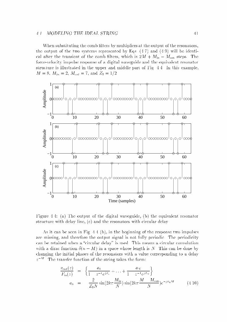
When substituting the comb �lters by multipliers at the output of the resonators,the output of the two systems represented by Eqs. (4.7) and (4.9) will be identi-cal after the transient of the comb �lters, which is 2M +Min �Mout steps. Theforce-velocity impulse response of a digital waveguide and the equivalent resonatorstructure is illustrated in the upper and middle part of Fig. 4.4. In this example,M = 8, Min = 2, Mout = 7, and Z0 = 1=2.

0 10 20 30 40 50 60−1

0

1

Am

plitu

de

(a)

0 10 20 30 40 50 60−1

0

1

Am

plitu

de

(b)

0 10 20 30 40 50 60−1

0

1

Time (samples)

Am

plitu

de

(c)

Figure 4.4: (a) The output of the digital waveguide, (b) the equivalent resonatorstructure with delay line, (c) and the resonators with circular delay.

As it can be seen in Fig. 4.4 (b), in the beginning of the response two impulsesare missing, and therefore the output signal is not fully periodic. The periodicitycan be retained when a �circular delay� is used. This means a circular convolutionwith a dirac function �(n�M) in a space whose length is N . This can be done bychanging the initial phases of the resonators with a value corresponding to a delayz�M . The transfer function of the string takes the form:

vout(z)

Fin(z)=

�a1

1� z�1ej#1+ : : :+

aN1 � z�1ej#N

�

ak = � 2

Z0Nsin(2k�

Min

N) sin(2k�

M �Mout

N)e�j#kM (4.10)

42 CHAPTER 4. PRINCIPLES OF STRING MODELING

The impulse response of the system is shown in Fig. 4.4 (c). Now in Fig. 4.3 A willrefer to a junction with input coe�cients ak to every branch and B reduces to asimple adder.

The impulse response of Eq. 4.10 can be formulated in the following way:

h(n) =N�1Xk=0

akej#kn =

N�1Xk=0

akej 2�Nkn (4.11)

which is the Inverse Discrete Fourier Transform of the ak coe�cients. Generally,when the poles of the resonators are equally distributed on the unit circle, theimpulse response of the digital waveguide and the initial amplitudes and phases ofthe resonators are related by the Discrete Fourier Transform. This holds for theideal string discussed above. This way the complex resonator coe�cients ak can becomputed by taking the DFT of the �rst N samples of the impulse response.

In the digital waveguide the behavior of the string between the nodes can becalculated by interpolation [Smith 1992; Laakso et al. 1996]. The inverse opera-tion of that is the deinterpolation [Välimäki et al. 1993; Välimäki 1995], where theexcitation force is introduced by fractional delay �lters between the nodes of thewaveguide. In the resonator implementation of Eq. (4.9) there is no need for suchoperations since by choosing proper input and output coe�cients for the resonators,Min and Mout can be arbitrary rational numbers.

In the case of multiple inputs and outputs, the input and output signals formvectors x and y, and the input and output coe�cients can be arranged to matricesA and B. The matrix R is diagonal and contains the transfer functions of theresonators. The output of the system is calculated in the following way:

y = BRAx Rkk =1

1 � z�1ej#k(4.12)

It is worth to note that in some cases the delay z�M of Eq. (4.9) cannot berealized with a circular delay as shown in Eq. (4.10). Equation (4.10) is useful onlywhen all the resonators are implemented. In the case of simulating some secondarye�ects of the piano sound, as it will be presented in Section 5.3, only some resonatorsare used. The solution for the problem will be discussed there.

In the simulation of string instruments, it is more important to know the forceexperienced by the termination (bridge) than the movement of the string. Thereason for this is that the sound is mainly radiated by the body or the soundboardand not the string, since the impedance matching between the string and the air isine�cient. From Eqs. (4.4) and (4.5) the force at the bridge Fbr will be:

F+ = v+Z0

F� = rFF+ = rFv

+Z0

Fbr = F+ + F� = (1 + rF )Z0v+ = 2Z0v

+ (4.13)

The transfer function from the excitation point to the bridge is:

Fbr

Fin=

1

1 � z�N

�1� z�2Min

�z�(M�Min) (4.14)

4.2. NON-IDEAL TERMINATION 43

The resonator coe�cients ak will take the form:

Fbr

Fin=

�a1

1 � z�1ej#1+ : : :+

aN1 � z�1ej#N

�z�M

ak = j2

Nsin(2k�

Min

N) (4.15)

where #k = (2k�)=N .The output of Eqs. (4.14) and (4.15) will di�er only in the �rstM+Min taps. The

delay z�M can be eliminated from Eq. (4.15) in the same way as shown in Eq. (4.10).Then the impulse response of the resonators and of the digital waveguide will be thesame from the �rst time instant.

4.2 Non-ideal termination

When the string is terminated by a �nite impedance Z > Z0, the absolute valueof the re�ection coe�cient rv will be somewhat lower than 1. If the terminationis purely resistive (Z is real and frequency independent), rv will be a real constantnumber. The waves traveling in the delay lines are multiplied by a constant factorevery time they pass through the termination. Consequently, all the harmonics willdecay exponentially with the same time coe�cient � . If one of the terminations iscompletely rigid and the other has an impedance of Z > Z0, the decay time of theharmonics will be the following:

� = � 1

f0 ln rF(4.16)

where rF is the force re�ection coe�cient (rF = �rv), f0 = N=fs is the fundamentalfrequency, fs refers to the sampling frequency, and N to the total length of thedelay line. The re�ection coe�cient rF can be calculated using Eq. (4.5). Eq. (4.16)was presented with relation to the decay times of the Karplus-Strong algorithm in[Ja�e and Smith 1983]. If none of the terminations are completely rigid, the rFused in Eq. (4.16) is the product of the re�ection coe�cients of the two sides. Theequivalent resonator bank will change in the radius of the poles since they moveslightly towards the origin:

Fbr

Fin=

�a1

1� z�1r1ej#1+ : : :+

aN1 � z�1rNej#N

�z�M

r1 = : : : = rN = (rF )1

N (4.17)

where #k = (2k�)=N , N = 2M and rk are the pole radii.The approximate decay times can be calculated in the same way for frequency

dependent rational impedance Z(z) with the help of Eqs. (4.5) and (4.16) at themodal frequencies. If e.g. the impedance of the termination decreases with frequency,the decay times of the higher harmonics will be smaller than those of the lower ones.

44 CHAPTER 4. PRINCIPLES OF STRING MODELING

If the slope of the function rF is small, the modal frequencies will not di�er fromthat of the in�nitely rigid termination signi�cantly.

By an arbitrary, complex termination the modal frequencies also change. A goodapproximation for these frequencies is:

'(#k)� #kN = �2k� (4.18)

where the �rst term '(#k) = arg(rF ) stands for the phase response introduced bythe impedance, and the second term refers to the phase of the delay line. Thephysical meaning of Eq. (4.18) is that a standing wave of the frequency #k has to�t in the string k=2, or in the delay line of the digital waveguide k times.

If the amplitude of rF is constant with respect to the frequency, Eq. (4.16) isexact. If not, the modal frequencies will be slightly in�uenced by the slope of jrF j.In our cases this di�erence can be neglected, since jrF j is close to 1 and its slope isvery small, thus it can be considered constant around the resonance frequencies ofthe digital waveguide.

If the impedance is not of an explicit form, the modal frequencies #k cannot becalculated directly. They can be estimated by the iterate use of Eq. (4.18) with astarting value of the ideal waveguide ('(#k) = 0). Precise results in determiningthe modal frequencies and decay times can be achieved by the fractional expansionof the whole transfer function. Because of the high order of the transfer function,numerical methods (such as the residue command in MATLAB) should be used,although these algorithms can easily give wrong results due to numerical instability.

4.3 The non-ideal string

In the general case, the wave equation of the string is similar to Eq. (4.1), but ithas to be extended by higher-order spatial- and time-derivate terms. The odd-ordertime-derivates are responsible for the losses and the even-order spatial-derivates forthe dispersion of the string [Smith 1993]. The latter means that the wave velocityof the sti� string will vary with the frequency. As a result, the partials will not beharmonic anymore.

Since we are observing the behavior of the string between two points (the inputand the output), the losses and dispersion can be lumped to one point [Smith 1992].As it was shown in the previous section, the in�uence of the termination can be easilytaken into account by a frequency dependent re�ection coe�cient rv. Hence, it isbene�cial to use the re�ection coe�cient for implementing the dispersion and lossesof the string as well. The re�ection coe�cients of the two sides can be transformedto one side of the string (rv = �rvleft � rvright), therefore on the other side only amultiplication by �1 is needed (see Fig. 4.5). This new re�ection coe�cient rvwill contain the losses and dispersion of the string on the one hand and the e�ectof the terminations on the other. Our task now is to determine this re�ectioncoe�cient from measurement data or analytical expressions. If it succeeds, thedigital waveguide will behave in the same way as the original system.

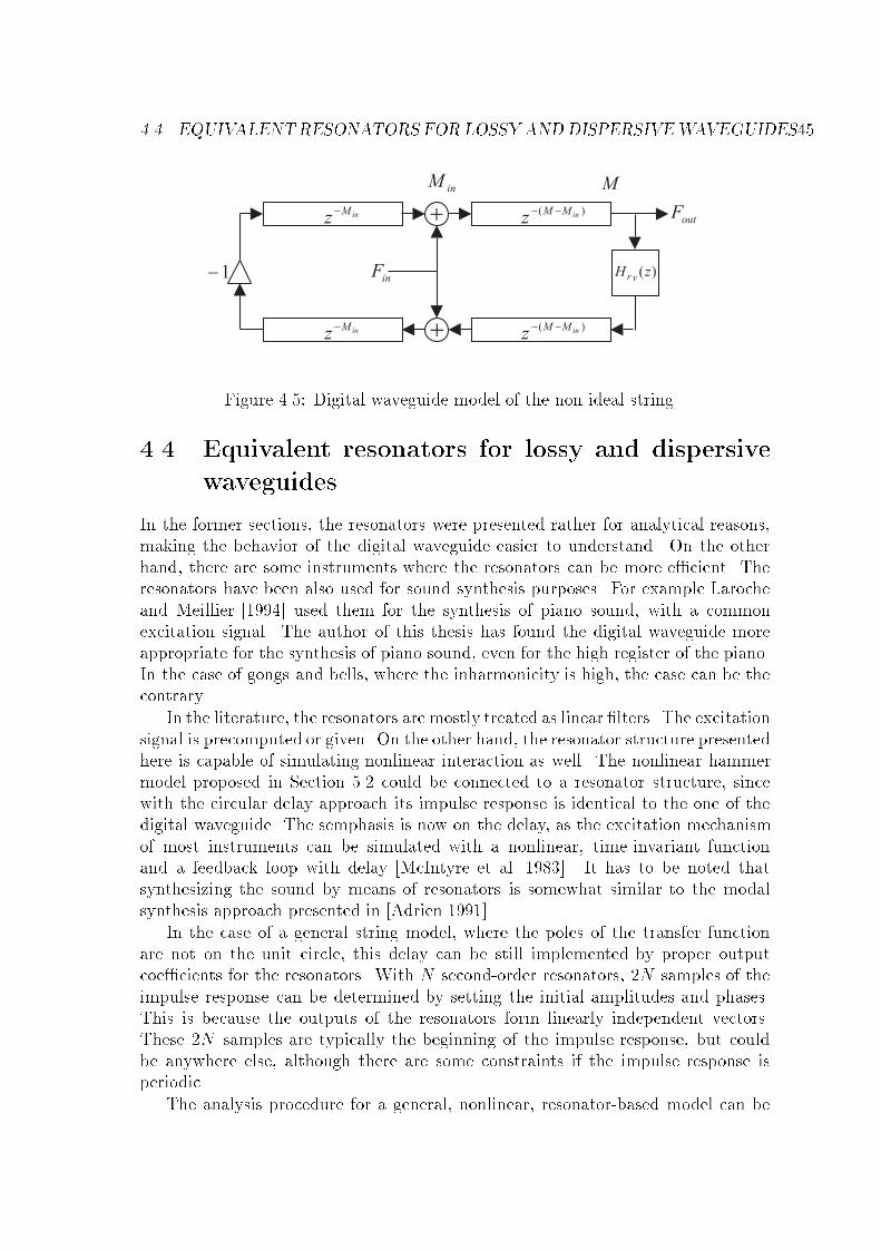
4.4. EQUIVALENTRESONATORS FOR LOSSY ANDDISPERSIVEWAVEGUIDES45

Figure 4.5: Digital waveguide model of the non-ideal string.

4.4 Equivalent resonators for lossy and dispersive

waveguides

In the former sections, the resonators were presented rather for analytical reasons,making the behavior of the digital waveguide easier to understand. On the otherhand, there are some instruments where the resonators can be more e�cient. Theresonators have been also used for sound synthesis purposes. For example Larocheand Meillier [1994] used them for the synthesis of piano sound, with a commonexcitation signal. The author of this thesis has found the digital waveguide moreappropriate for the synthesis of piano sound, even for the high register of the piano.In the case of gongs and bells, where the inharmonicity is high, the case can be thecontrary.

In the literature, the resonators are mostly treated as linear �lters. The excitationsignal is precomputed or given. On the other hand, the resonator structure presentedhere is capable of simulating nonlinear interaction as well. The nonlinear hammermodel proposed in Section 5.2 could be connected to a resonator structure, sincewith the circular delay approach its impulse response is identical to the one of thedigital waveguide. The semphasis is now on the delay, as the excitation mechanismof most instruments can be simulated with a nonlinear, time-invariant functionand a feedback loop with delay [McIntyre et al. 1983]. It has to be noted thatsynthesizing the sound by means of resonators is somewhat similar to the modalsynthesis approach presented in [Adrien 1991].

In the case of a general string model, where the poles of the transfer functionare not on the unit circle, this delay can be still implemented by proper outputcoe�cients for the resonators. With N second-order resonators, 2N samples of theimpulse response can be determined by setting the initial amplitudes and phases.This is because the outputs of the resonators form linearly independent vectors.These 2N samples are typically the beginning of the impulse response, but couldbe anywhere else, although there are some constraints if the impulse response isperiodic.

The analysis procedure for a general, nonlinear, resonator-based model can be

46 CHAPTER 4. PRINCIPLES OF STRING MODELING

the following: �rst, the partial frequencies and decay times are determined. Thenthe impulse response of the acoustical resonator (string, bell, etc.) is estimated.By using the frequency and decay time parameters of the N resonators, togetherwith 2N samples of the impulse response, 2N linear equations can be written. Oneresonator corresponds to two equations, since both the initial amplitude and phaseare free parameters. These parameters can be determined by using resonators, e.g.,with initial amplitude of 1 and initial phases of 0 and 90 degrees in the linearequations.

4.5 The digital waveguide as an approximation

By reversing the order of ideas, the digital waveguide can be viewed as the approx-imation of the resonator bank. If the fractions of the resonators are brought to acommon denominator, the resulting system will be an exact copy of the resonatorbank with respect to the input-output behavior. In the general case, the delay linedisappears and the whole digital waveguide will become a re�ection-coe�cient �lterwith feedback. In this case the number of operations remains the same. On thecontrary, if we let the speci�cation for the modal frequencies and decay times to besomewhat loose, the computational complexity can be radically reduced. Nearly har-monic signals can be produced by using a delay line and, e.g., a 10th-order re�ection�lter instead of using 100 resonators. While in the resonator-bank implementationthe computational complexity depends on the number of the harmonics, in the digi-tal waveguide it depends on the precision of the approximation. The human auditorysystem seems to be more tolerant for slight inaccuracies than for completely missingharmonics. Consequently, the digital waveguide is a more e�cient tool for modelingnearly harmonic sounds. On the other hand, when the generation of a small numberof partials is needed, the resonator bank can be a more e�cient approach. This isthe case for example when simulating the two-stage decay of the piano sound.

4.6 Conclusion

We overviewed a computationally very e�cient technique for modeling the stringbehavior, the digital waveguide model. Its e�ciency comes from the fact that lossesand dispersion of the string-termination system are lumped to one point. Therefore,the string simulation loop consists of two delay lines and one re�ection �lter. Bymathematically reformulating the transfer function of the digital waveguide, theequivalent resonator bank structure was presented. Methods for calculating theparameters of the resonator bank were also given. A new feature of this approachis that the resonator bank can be used for simulating nonlinear interaction, sinceits behavior is the same as that of the digital waveguide. This can be useful forthe modeling of instruments with high inharmonicity, such as mallet percussioninstruments, gongs, or bells.

Chapter 5

Model structure

First, the general structure of the piano model is presented. Then separate partsof the model are described in detail. A new multi-rate hammer model and a noveltechnique for simulating beating and two-stage decay are proposed. A simple tech-nique for the realistic simulation of the attack sound of the piano is also outlined.The last part of the chapter deals with the issues of practical implementation andpresents a multi-rate piano model. The calibration of the model and the estimationof the parameters are discussed in Chapter 6.

5.1 General structure of the piano model

Since the physical modeling approach tries to simulate the structure of the instru-ment, and not the sound itself, the piano model consists of the same parts as thereal piano. The structure of the model is displayed in Fig. 5.1. The �rst step ofthe sound production mechanism is the excitation, which is the hammer strike inthe case of the piano. The resulting signal propagates to the string, which deter-mines the fundamental frequency of the tone. The periodic output signal is �lteredthrough the radiator, covering the e�ect of the soundboard.

Figure 5.1 shows that the interaction between the string and the excitationis bidirectional, since the hammer force also depends on the string displacement[Fletcher and Rossing 1998]. On the other hand, there is no feedback from thesoundboard to the string. Although the impedance of the bridge and the sound-board in�uence the decay times of the partials, this e�ect is taken into account inthe string model. At this point, our model di�ers from the real piano: the two func-tions of the soundboard, namely, the determination of the decay times and formingthe spectrum, are put to separate parts of the model. This way, the e�ect of thesoundboard can be treated as a linear �ltering operation [Smith 1983; Välimäki etal. 1996].

The hammer model solves the di�erential equation of the hammer in discretetime. This part of the model is responsible for shaping the initial spectrum, byproviding the excitation to the string model. On the other hand, it has no in�uenceon the time dependent evolution of the spectra in the decay part of the sound. Its

47

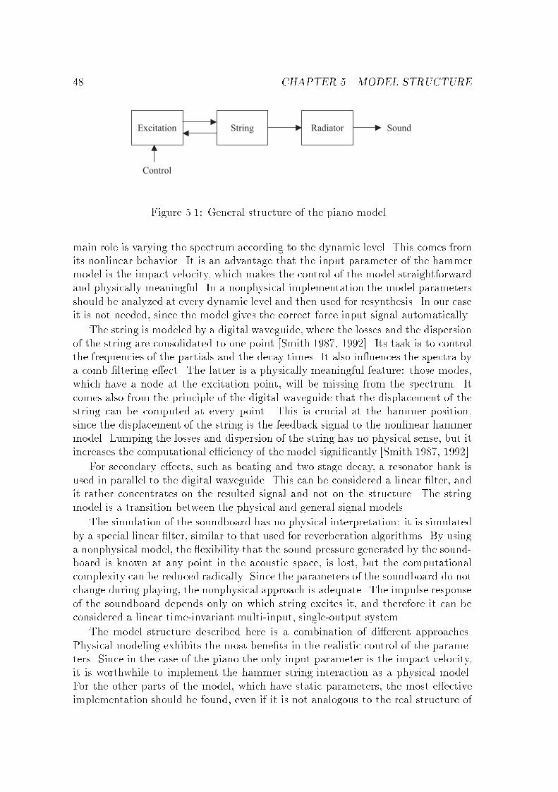
48 CHAPTER 5. MODEL STRUCTURE

Figure 5.1: General structure of the piano model.

main role is varying the spectrum according to the dynamic level. This comes fromits nonlinear behavior. It is an advantage that the input parameter of the hammermodel is the impact velocity, which makes the control of the model straightforwardand physically meaningful. In a nonphysical implementation the model parametersshould be analyzed at every dynamic level and then used for resynthesis. In our caseit is not needed, since the model gives the correct force input signal automatically.

The string is modeled by a digital waveguide, where the losses and the dispersionof the string are consolidated to one point [Smith 1987, 1992]. Its task is to controlthe frequencies of the partials and the decay times. It also in�uences the spectra bya comb �ltering e�ect. The latter is a physically meaningful feature: those modes,which have a node at the excitation point, will be missing from the spectrum. Itcomes also from the principle of the digital waveguide that the displacement of thestring can be computed at every point. This is crucial at the hammer position,since the displacement of the string is the feedback signal to the nonlinear hammermodel. Lumping the losses and dispersion of the string has no physical sense, but itincreases the computational e�ciency of the model signi�cantly [Smith 1987, 1992].

For secondary e�ects, such as beating and two stage decay, a resonator bank isused in parallel to the digital waveguide. This can be considered a linear �lter, andit rather concentrates on the resulted signal and not on the structure. The stringmodel is a transition between the physical and general signal models.

The simulation of the soundboard has no physical interpretation: it is simulatedby a special linear �lter, similar to that used for reverberation algorithms. By usinga nonphysical model, the �exibility that the sound pressure generated by the sound-board is known at any point in the acoustic space, is lost, but the computationalcomplexity can be reduced radically. Since the parameters of the soundboard do notchange during playing, the nonphysical approach is adequate. The impulse responseof the soundboard depends only on which string excites it, and therefore it can beconsidered a linear time-invariant multi-input, single-output system.

The model structure described here is a combination of di�erent approaches.Physical modeling exhibits the most bene�ts in the realistic control of the parame-ters. Since in the case of the piano the only input parameter is the impact velocity,it is worthwhile to implement the hammer-string interaction as a physical model.For the other parts of the model, which have static parameters, the most e�ectiveimplementation should be found, even if it is not analogous to the real structure of

5.2. MODELING THE HAMMER AND THE DAMPERS 49

the piano.

5.2 Modeling the hammer and the dampers

First, the di�erent hammer models found in the literature are reviewed. Then, theproblems for feeding the interaction force into the digital waveguide are discussed,and for avoiding these problems, new solutions are proposed. After that, the hammerand damper models are presented1.

The hammer is modeled by a linear di�erence equation and an instantaneousnonlinearity. The di�erence equation calculates the movement of the hammer andthe nonlinear part accounts for the felt characteristic. An advantage of the nonlinearmodel is the dynamic variation of the timbre, according to the impact velocity. Anovel multi-rate hammer model is presented for assuring the stability of the model.The e�ect of dampers is simulated with a linear �lter. A new nonlinear dampermodel is also proposed, which is based on the hammer model.

5.2.1 Overview of prior work

The hammer is generally considered as a mass connected to a nonlinear spring[see, e.g., Boutillon 1988]. As it has an initial velocity, it hits the string. Thespring compresses, and the interaction force pushes the hammer away from thestring. The most straightforward approach for modeling the hammer is discretizingthe di�erential equation of the mass. The position of the hammer is obtained bymultiplying the interaction force with a scalar and integrating twice with respect totime. The nonlinear felt characteristic (see Eq. 2.1) can be directly implemented ina discrete form. This approach was taken in [Chaigne and Askenfelt 1994a,b], wherethe hammer was connected to a �nite-di�erence model of the string. Simulationresults showed good agreement with the measured data. Borin et al. [1992] appliedthe same kind of power law model to the digital waveguide. An advantage of thistechnique is its simplicity, and, as it is a nonlinear model, the spectrum of itsoutput varies dynamically according to the impact velocity. The problem withthis straightforward approach is that for high sti�ness and initial velocity values thehammer model can become unstable, mostly in the high note range of the piano[Borin and De Poli 1996; Borin et al. 1997].

A solution to this problem can be found in [Borin and De Poli 1996; Borin etal. 1997]. It is based on the separation of known and unknown terms, and solvingan implicit equation. For integer sti�ness exponents (p = 2, 3, or 4 in Eq. 2.1)an analytic solution of the implicit equation can be derived. They also introducethe hysteresis to their model by discretizing the equations of [Stulov 1995]. Thedrawback of the model is that the computation of the interaction force is quitecomplicated, even for a sti�ness exponent value p = 2. The model cannot be used

1parts of this section are also published in [Bank 2000]

50 CHAPTER 5. MODEL STRUCTURE

with noninteger p values, since the solution of an implicit equation would take toomany computations.

An elegant solution for the hammer model based on the traveling wave decom-position of the mass-spring system was proposed in [Van Duyne et al. 1994]. There,a distributed hammer model was attached to the string by a scattering junction.The distributed model was derived for a linear spring. The nonlinear character-istic of the felt was taken into account by reading the sti�ness coe�cient from alookup-table, according to the compression of the felt. Hysteresis was modeled byo�setting the pointer in the table, corresponding to the velocity of felt compression.The disadvantage of this technique lies in its complexity.

In [Smith and Van Duyne 1995; Van Duyne and Smith 1995], a linear hammermodel was used. The hammer was modeled by a linear �lter, whose parameterswere determined by nonlinear simulation. The advantage of the linear approach isthat the soundboard �lter can be commuted through the string and the hammer[Karjalainen and Välimäki 1993; Smith 1993]. Hence, the soundboard need notbe implemented as a �lter, but as a wavetable, whose content is played into thestring through the hammer �lter. This reduces the computational complexity of thesoundboard model largely. A drawback is that the hammer �lter has to be designedfor all of the strings and at every dynamic level. Accordingly, the nice feature of thenonlinear model, that it responds to the initial velocity in a physically meaningfulway, is lost. Moreover, the restrike of the string cannot be simulated correctly.

5.2.2 The discontinuity problem: nonlinear interaction in the

digital waveguide

There are two di�erent tasks when connecting the hammer to the string. One isintroducing the interaction force to the digital waveguide and the other is determin-ing the displacement of the string, since that is the feedback signal to the hammermodel. These can be done as shown in Fig. 4.2, where Mout = Min for this case.The displacement of the string can be determined by integrating the velocity signalvout. However, there is a problem with this simple approach. Here we will deal withthe problem thoroughly, since it has not been discussed in the literature.

Let us assume that the string is in�nite, or terminated by a Z0 impedance, i.e.,there is no re�ection from the terminations. There are two possibilities for connect-ing the hammer model to the digital waveguide, according to Fig. 4.2. One is �rstto read the string velocity from the delay lines and then to add the excitation signalto the cells. After this, the delay lines are shifted. In this case, the velocity whichis read from the cells at the hammer position will be always zero. Consequently, allparts of the string will be moving, but not the excitation point. Since the feedbackto the hammer model is coming from the displacement of the excitation point, thehammer will behave as if it was bouncing to a rigid wall. Obviously, this method isnot appropriate.

The other approach is the opposite: �rst we add the excitation signal to thedelay cells at the position of the hammer, then read the string velocity, and shift

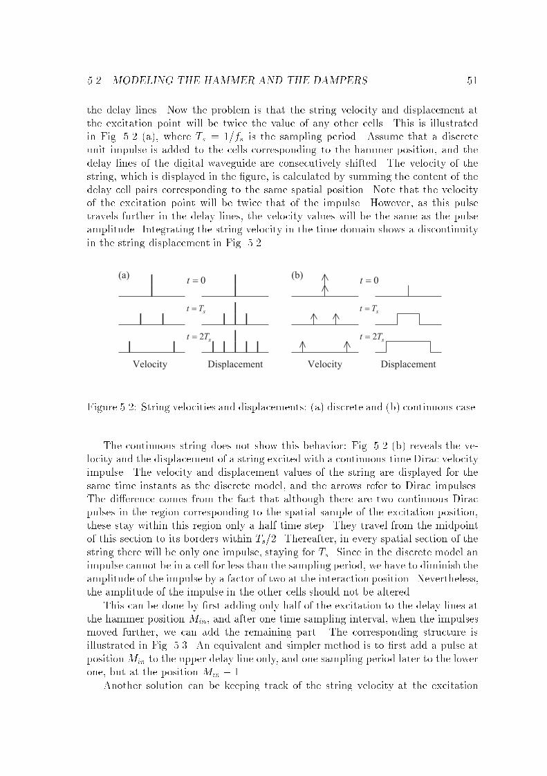
5.2. MODELING THE HAMMER AND THE DAMPERS 51

the delay lines. Now the problem is that the string velocity and displacement atthe excitation point will be twice the value of any other cells. This is illustratedin Fig. 5.2 (a), where Ts = 1=fs is the sampling period. Assume that a discreteunit impulse is added to the cells corresponding to the hammer position, and thedelay lines of the digital waveguide are consecutively shifted. The velocity of thestring, which is displayed in the �gure, is calculated by summing the content of thedelay cell pairs corresponding to the same spatial position. Note that the velocityof the excitation point will be twice that of the impulse. However, as this pulsetravels further in the delay lines, the velocity values will be the same as the pulseamplitude. Integrating the string velocity in the time domain shows a discontinuityin the string displacement in Fig. 5.2.

Figure 5.2: String velocities and displacements: (a) discrete and (b) continuous case.

The continuous string does not show this behavior: Fig. 5.2 (b) reveals the ve-locity and the displacement of a string excited with a continuous-time Dirac velocityimpulse. The velocity and displacement values of the string are displayed for thesame time instants as the discrete model, and the arrows refer to Dirac impulses.The di�erence comes from the fact that although there are two continuous Diracpulses in the region corresponding to the spatial sample of the excitation position,these stay within this region only a half time step. They travel from the midpointof this section to its borders within Ts=2. Thereafter, in every spatial section of thestring there will be only one impulse, staying for Ts. Since in the discrete model animpulse cannot be in a cell for less than the sampling period, we have to diminish theamplitude of the impulse by a factor of two at the interaction position. Nevertheless,the amplitude of the impulse in the other cells should not be altered.

This can be done by �rst adding only half of the excitation to the delay lines atthe hammer position Min, and after one time sampling-interval, when the impulsesmoved further, we can add the remaining part. The corresponding structure isillustrated in Fig. 5.3. An equivalent and simpler method is to �rst add a pulse atposition Min to the upper delay line only, and one sampling period later to the lowerone, but at the position Min � 1.

Another solution can be keeping track of the string velocity at the excitation

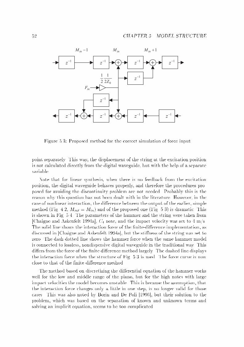
52 CHAPTER 5. MODEL STRUCTURE

Figure 5.3: Proposed method for the correct simulation of force input.

point separately. This way, the displacement of the string at the excitation positionis not calculated directly from the digital waveguide, but with the help of a separatevariable.

Note that for linear synthesis, when there is no feedback from the excitationposition, the digital waveguide behaves properly, and therefore the procedures pro-posed for avoiding the discontinuity problem are not needed. Probably this is thereason why this question has not been dealt with in the literature. However, in thecase of nonlinear interaction, the di�erence between the output of the earlier, simplemethod (Fig. 4.2, Mout = Min) and of the proposed one (Fig. 5.3) is dramatic. Thisis shown in Fig. 5.4. The parameters of the hammer and the string were taken from[Chaigne and Askenfelt 1994a], C4 note, and the impact velocity was set to 4 m/s.The solid line shows the interaction force of the �nite-di�erence implementation, asdiscussed in [Chaigne and Askenfelt 1994a], but the sti�ness of the string was set tozero. The dash-dotted line shows the hammer force when the same hammer modelis connected to lossless, nondispersive digital waveguide in the traditional way. Thisdi�ers from the force of the �nite di�erence method largely. The dashed line displaysthe interaction force when the structure of Fig. 5.3 is used. The force curve is nowclose to that of the �nite di�erence method.

The method based on discretizing the di�erential equation of the hammer workswell for the low and middle range of the piano, but for the high notes with largeimpact velocities the model becomes unstable. This is because the assumption, thatthe interaction force changes only a little in one step, is no longer valid for thosecases. This was also noted by Borin and De Poli [1996], but their solution to theproblem, which was based on the separation of known and unknown terms andsolving an implicit equation, seems to be too complicated.

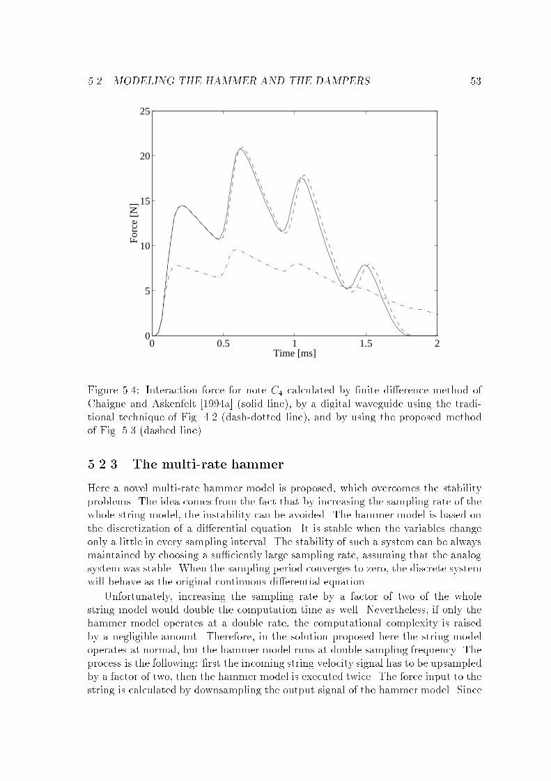
5.2. MODELING THE HAMMER AND THE DAMPERS 53

0 0.5 1 1.5 20

5

10

15

20

25

Time [ms]

For

ce [N

]

Figure 5.4: Interaction force for note C4 calculated by �nite di�erence method ofChaigne and Askenfelt [1994a] (solid line), by a digital waveguide using the tradi-tional technique of Fig. 4.2 (dash-dotted line), and by using the proposed methodof Fig. 5.3 (dashed line).

5.2.3 The multi-rate hammer

Here a novel multi-rate hammer model is proposed, which overcomes the stabilityproblems. The idea comes from the fact that by increasing the sampling rate of thewhole string model, the instability can be avoided. The hammer model is based onthe discretization of a di�erential equation. It is stable when the variables changeonly a little in every sampling interval. The stability of such a system can be alwaysmaintained by choosing a su�ciently large sampling rate, assuming that the analogsystem was stable. When the sampling period converges to zero, the discrete systemwill behave as the original continuous di�erential equation.

Unfortunately, increasing the sampling rate by a factor of two of the wholestring model would double the computation time as well. Nevertheless, if only thehammer model operates at a double rate, the computational complexity is raisedby a negligible amount. Therefore, in the solution proposed here the string modeloperates at normal, but the hammer model runs at double sampling frequency. Theprocess is the following: �rst the incoming string velocity signal has to be upsampledby a factor of two, then the hammer model is executed twice. The force input to thestring is calculated by downsampling the output signal of the hammer model. Since

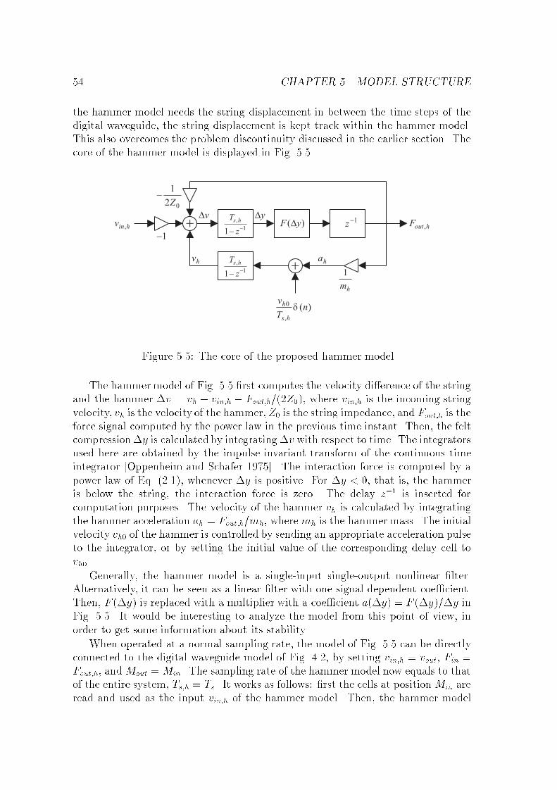
54 CHAPTER 5. MODEL STRUCTURE

the hammer model needs the string displacement in between the time steps of thedigital waveguide, the string displacement is kept track within the hammer model.This also overcomes the problem discontinuity discussed in the earlier section. Thecore of the hammer model is displayed in Fig. 5.5.

Figure 5.5: The core of the proposed hammer model.

The hammer model of Fig. 5.5 �rst computes the velocity di�erence of the stringand the hammer �v = vh � vin;h � Fout;h=(2Z0), where vin;h is the incoming stringvelocity, vh is the velocity of the hammer,Z0 is the string impedance, and Fout;h is theforce signal computed by the power law in the previous time instant. Then, the feltcompression�y is calculated by integrating�v with respect to time. The integratorsused here are obtained by the impulse-invariant transform of the continuous timeintegrator [Oppenheim and Schafer 1975]. The interaction force is computed by apower law of Eq. (2.1), whenever �y is positive. For �y < 0, that is, the hammeris below the string, the interaction force is zero. The delay z�1 is inserted forcomputation purposes. The velocity of the hammer vh is calculated by integratingthe hammer acceleration ah = Fout;h=mh, where mh is the hammer mass. The initialvelocity vh0 of the hammer is controlled by sending an appropriate acceleration pulseto the integrator, or by setting the initial value of the corresponding delay cell tovh0.

Generally, the hammer model is a single-input single-output nonlinear �lter.Alternatively, it can be seen as a linear �lter with one signal dependent coe�cient.Then, F (�y) is replaced with a multiplier with a coe�cient a(�y) = F (�y)=�y inFig. 5.5. It would be interesting to analyze the model from this point of view, inorder to get some information about its stability.

When operated at a normal sampling rate, the model of Fig. 5.5 can be directlyconnected to the digital waveguide model of Fig. 4.2, by setting vin;h = vout, Fin =Fout;h, and Mout = Min. The sampling rate of the hammer model now equals to thatof the entire system, Ts;h = Ts. It works as follows: �rst the cells at position Min areread and used as the input vin;h of the hammer model. Then, the hammer model

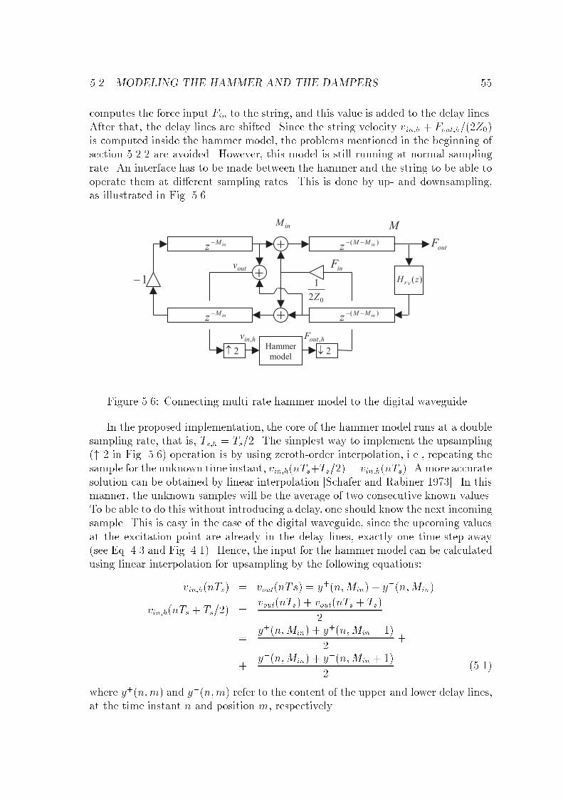
5.2. MODELING THE HAMMER AND THE DAMPERS 55

computes the force input Fin to the string, and this value is added to the delay lines.After that, the delay lines are shifted. Since the string velocity vin;h + Fout;h=(2Z0)is computed inside the hammer model, the problems mentioned in the beginning ofsection 5.2.2 are avoided. However, this model is still running at normal samplingrate. An interface has to be made between the hammer and the string to be able tooperate them at di�erent sampling rates. This is done by up- and downsampling,as illustrated in Fig. 5.6.

Figure 5.6: Connecting multi-rate hammer model to the digital waveguide.

In the proposed implementation, the core of the hammer model runs at a doublesampling rate, that is, Ts;h = Ts=2. The simplest way to implement the upsampling(" 2 in Fig. 5.6) operation is by using zeroth-order interpolation, i.e., repeating thesample for the unknown time instant, vin;h(nTs+Ts=2) = vin;h(nTs). A more accuratesolution can be obtained by linear interpolation [Schafer and Rabiner 1973]. In thismanner, the unknown samples will be the average of two consecutive known values.To be able to do this without introducing a delay, one should know the next incomingsample. This is easy in the case of the digital waveguide, since the upcoming valuesat the excitation point are already in the delay lines, exactly one time-step away(see Eq. 4.3 and Fig. 4.1). Hence, the input for the hammer model can be calculatedusing linear interpolation for upsampling by the following equations:

vin;h(nTs) = vout(nTs) = y+(n;Min) + y�(n;Min)

vin;h(nTs + Ts=2) =vout(nTs) + vout(nTs + Ts)

2

=y+(n;Min) + y+(n;Min � 1)

2+

+y�(n;Min) + y�(n;Min + 1)

2(5.1)

where y+(n;m) and y�(n;m) refer to the content of the upper and lower delay lines,at the time instant n and position m, respectively.

56 CHAPTER 5. MODEL STRUCTURE

The force input for the string is computed by simply averaging the two outputsamples of the force model, i.e., Fin(nTs) = (Fout;h(nTs) + Fout;h(nTs + Ts=2))=2.

The analysis of the new method

The multi-rate method has proven to be a robust solution for modeling the hammer.For note C7 (2090 Hz), the hammer starts to be unstable for an impact velocity asmuch as 20 m/s, which is three times of the maximal velocity which can arise in areal piano. By using the single-rate model, it is already unstable at around 5 m/s.

In Fig. 5.7 the interaction force is shown for note C5 (522 Hz). For the simula-tion, an ideal digital waveguide model was used, without any dispersion or losses.The parameters of the hammer were taken from [Chaigne and Askenfelt 1994a], C4

hammer. The impact velocity was vh0 = 6 m/s. The dash-dotted line refers tothe single-rate hammer model with fs = 44:1 kHz. The solid line shows the forceof the single-rate model, but the whole digital waveguide model is run at a doublesample rate, that is, fs = 88:2 kHz. This is our reference structure. The dashedline in Fig 5.7 is the force of the multi-rate implementation, by using fs = 44:1 kHzfor the waveguide model. It can be seen that the traditional technique operatingat normal sampling rate goes unstable, while the output of the proposed multi-rate hammer model coincides with the output of the single-rate model operating atdouble sampling frequency.

Surprisingly, the multi-rate method is more stable than the single-rate operatingat double sampling rate. For the same string and hammer parameters as in theprevious example, the single-rate model at double sampling frequency goes unstablefor vh0 > 18 m/s, the multi-rate model is still stable until vh;0 = 42 m/s. This isbecause the multi-rate model functions like the single-rate model running at dou-ble sampling frequency, but with lowpass-�ltering at the input and output of thehammer model. This comes from the up- and downsampling: the hammer modeloperates at 2fs, but its input vin;h is upsampled from a signal vout whose samplingrate is fs. Consequently, the input cannot contain strong frequency componentshigher than fs=2. In this way, the incoming high frequency components, which aremainly responsible for stability problems, are suppressed.

Hysteresis can be easily included in the model by discretizing the equations of[Stulov 1995]. This was done by the bilinear transform in [Borin and De Poli 1996].The �rst-order IIR �lter obtained that way is then cascaded with the instantaneousnonlinearity F (�y) in Fig. 5.5.

To conclude, the new multi-rate hammer model proposed here, overcomes thediscontinuity problem discussed in Section 5.2.2. This is done by computing thestring displacement at the excitation point within the hammer model. The stabilityof the hammer model is ensured by the multi-rate approach. This makes the modelmore stable since higher sampling rate yields a better discrete time approximationof the di�erential equation. It is also because the high frequency components of theinput signal, which are mainly responsible for instability problems, are suppressedby the linear interpolation. Another bene�t of the model is that it is simple, easy to

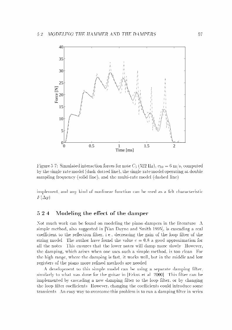
5.2. MODELING THE HAMMER AND THE DAMPERS 57

0 0.5 1 1.5 20

5

10

15

20

25

30

35

40

Time [ms]

For

ce [N

]

Figure 5.7: Simulated interaction forces for note C5 (522 Hz), vh0 = 6m/s, computedby the single-rate model (dash-dotted line), the single-rate model operating at doublesampling frequency (solid line), and the multi-rate model (dashed line).

implement, and any kind of nonlinear function can be used as a felt characteristicF (�y).

5.2.4 Modeling the e�ect of the damper

Not much work can be found on modeling the piano dampers in the literature. Asimple method, also suggested in [Van Duyne and Smith 1995], is cascading a realcoe�cient to the re�ection �lter, i.e., decreasing the gain of the loop �lter of thestring model. The author have found the value c = 0:8 a good approximation forall the notes. This ensures that the lower notes will damp more slowly. However,the damping, which arises when one uses such a simple method, is too clean. Forthe high range, where the damping is fast, it works well, but in the middle and lowregisters of the piano more re�ned methods are needed.

A development to this simple model can be using a separate damping �lter,similarly to what was done for the guitar in [Erkut et al. 2000]. This �lter can beimplemented by cascading a new damping �lter to the loop �lter, or by changingthe loop �lter coe�cients. However, changing the coe�cients could introduce sometransients. An easy way to overcome this problem is to run a damping �lter in series

58 CHAPTER 5. MODEL STRUCTURE

with the loop �lter. When the key is released, one has to simply switch from theoutput of the loop �lter to the output of the damping �lter, whose state variable isalready trained by the incoming samples [Välimäki and Laakso 1998]. The one-pole�lter approach gives good results for the high and middle register, but the roughnessof the damping of low piano strings is not reproduced.

5.2.5 The nonlinear damper model

The problem of these simple approaches, namely, changing the loop gain or cascadinga damping �lter, is that they are unable to simulate a characteristic feature of thedamping. The feature is that every 7th partial is damped ine�ciently, since thedamper cannot act well on a mode which has a node at the damper position (seeFig. 6.1). The di�erence can be heard especially at the lowest two octaves of thepiano. By using the physical modeling approach, this feature could also be modeled.

The proposed nonlinear damper model operates with the same architecture ofFig. 5.5, although its parameters have to be changed. As the hammer hits the stringfrom downwards, and the dampers fall on the string from upwards, the signs of thesignals in the input and output of the hammer model have to be inverted. Thegravity force, which pushes the damper to the string, can be simulated by addinga constant value to the hammer acceleration at every time instant. The mh valueand the F (�y) function have to be also changed. The initial velocity of the dampervh0 is set to zero. Since the main feature of the damper is dissipating energy, losseshave to be introduced to the model. The easiest way to do that is adding hysteresisto the felt, by cascading a highpass �lter with the output of the nonlinearity, as wasdone for the hammer in [Borin and De Poli 1996]. Another way can be to renderthe interaction force dependent on the velocity di�erence �v of the string and thehammer. Then the force is calculated by F (�v;�y).

The main bene�t of the model is that the slower damping of every partial, whichhas a node at the damper position, is modeled automatically. This comes from theprinciple of the physical modeling approach. Another advantage is that now thehammers and the dampers are simulated by the same part of the piano model. Aserious drawback is that the calibration of such a physical damper model can beproblematic. Unfortunately, there has been no data in the literature concerningthe damper characteristics of real pianos. This model has not been implemented inpractice, due to the previous reason. However, after conducting some measurementon piano dampers, the author plans to experiment with this nonlinear model.

5.3 The string model

The behavior of a piano string is simulated by a digital waveguide, mostly because ofpractical reasons. The equivalent resonator structure presented in Chapter 4 couldgive the same sound output, but it is computationally more expensive. It will beshown later in Section 5.3.3 that the resonators can be useful in modeling some

5.3. THE STRING MODEL 59

details of the piano sound.As discussed previously in connection with the hammermodel, the digital waveg-

uide has an important role in determining the excitation signal. Its other task islinear �ltering: it controls the frequencies and decay rates of the partials and itintroduces a comb-�ltering e�ect, thus also a�ects the short-time spectrum. If thesamples of the excitation signal are recorded and then fed to the digital waveguide,the same output will arise. This way the two functions of the digital waveguide,namely, determining the excitation and linear �ltering, can be separated. In thischapter, for didactical reasons, the digital waveguide is considered as a linear �lterand the excitation signal is assumed to be given.

5.3.1 The basic string model

The basic string model consists of a digital waveguide shown in Fig. 4.5 in Chapter 4.The fundamental frequency of the note and the frequency distribution of the partialsare determined by the delay line length M and the phase delay of the re�ection�lter Hrv . The decay times of the partials are controlled by the amplitude transferfunction of the re�ection �lter. The estimation of these parameters and methodsfor re�ection �lter design will be discussed in the next chapter. The basic stringmodel is capable of simulating pure exponentially decaying envelopes. Therefore itis unable to reproduce the beating and two-stage decay found in real piano tones.The physics of these two phenomena were discussed in Chapter 2.

5.3.2 Methods for beating and two-stage decay simulation

Here we review the methods previously presented in the literature.By using two digital waveguides in parallel for one note, the beating and two-

stage decay can be simulated in a simple way. If the fundamental frequencies ofthe two digital waveguides are di�erent, beating results, and if their decay timesare di�erent, two-stage decay will occur in the sound. The two digital waveguidescan be coupled with real coe�cients [Karjalainen et al. 1998]. Figure 5.8 shows thiscon�guration, where Sv(z) and Sh(z) are the two string models. The g parameterscontrol the input and output amplitudes of the digital waveguides and determinethe amount of coupling. The problem with this method is that the envelopes of thedi�erent partials will be similar, which is not the case for real piano tones. It alsoincreases the computational complexity by a factor of two compared to the basicstring model.

Another approach was taken by Smith [1993]. In his approximation, two idealstrings are coupled to the same termination, and all the losses are lumped to thebridge impedance Z. The structure is shown in Fig. 5.9. This comes from theassumption that all the losses come from the bridge, which is a rough approximation.By using one coupling �lter Hc for calculating the velocity of the bridge, the re�ectedvelocity waves v�1 and v�2 of the strings can be computed by subtracting the incomingwaves v+1 and v+2 from the bridge velocity vbr. The allpass �lters Hap1 and Hap2 still

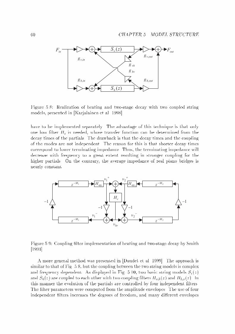
60 CHAPTER 5. MODEL STRUCTURE

Figure 5.8: Realization of beating and two-stage decay with two coupled stringmodels, presented in [Karjalainen et al. 1998].

have to be implemented separately. The advantage of this technique is that onlyone loss �lter Hc is needed, whose transfer function can be determined from thedecay times of the partials. The drawback is that the decay times and the couplingof the modes are not independent. The reason for this is that shorter decay timescorrespond to lower terminating impedance. Thus, the terminating impedance willdecrease with frequency to a great extent resulting in stronger coupling for thehigher partials. On the contrary, the average impedance of real piano bridges isnearly constant.

Figure 5.9: Coupling �lter implementation of beating and two-stage decay by Smith[1993].

A more general method was presented in [Daudet et al. 1999]. The approach issimilar to that of Fig. 5.8, but the coupling between the two string models is complexand frequency dependent. As displayed in Fig. 5.10, two basic string models Sv(z)and Sh(z) are coupled to each other with two coupling �ltersHv;h(z) and Hh;v(z). Inthis manner the evolution of the partials are controlled by four independent �lters.The �lter parameters were computed from the amplitude envelopes. The use of fourindependent �lters increases the degrees of freedom, and many di�erent envelopes

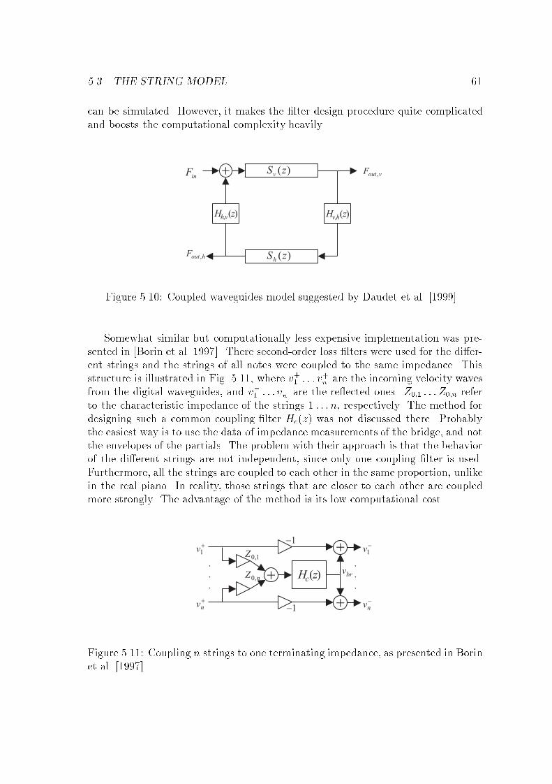
5.3. THE STRING MODEL 61

can be simulated. However, it makes the �lter design procedure quite complicatedand boosts the computational complexity heavily.

Figure 5.10: Coupled waveguides model suggested by Daudet et al. [1999].

Somewhat similar but computationally less expensive implementation was pre-sented in [Borin et al. 1997]. There second-order loss �lters were used for the di�er-ent strings and the strings of all notes were coupled to the same impedance. Thisstructure is illustrated in Fig. 5.11, where v+1 : : : v

+n are the incoming velocity waves

from the digital waveguides, and v�1 : : : v�

n are the re�ected ones. Z0;1 : : : Z0;n referto the characteristic impedance of the strings 1 : : : n, respectively. The method fordesigning such a common coupling �lter Hc(z) was not discussed there. Probablythe easiest way is to use the data of impedance measurements of the bridge, and notthe envelopes of the partials. The problem with their approach is that the behaviorof the di�erent strings are not independent, since only one coupling �lter is used.Furthermore, all the strings are coupled to each other in the same proportion, unlikein the real piano. In reality, those strings that are closer to each other are coupledmore strongly. The advantage of the method is its low computational cost.

Figure 5.11: Coupling n strings to one terminating impedance, as presented in Borinet al. [1997].

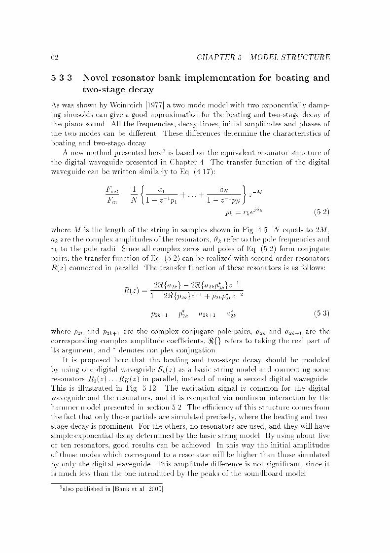
62 CHAPTER 5. MODEL STRUCTURE

5.3.3 Novel resonator bank implementation for beating and

two-stage decay

As was shown by Weinreich [1977] a two mode model with two exponentially damp-ing sinusoids can give a good approximation for the beating and two-stage decay ofthe piano sound. All the frequencies, decay times, initial amplitudes and phases ofthe two modes can be di�erent. These di�erences determine the characteristics ofbeating and two-stage decay.

A new method presented here2 is based on the equivalent resonator structure ofthe digital waveguide presented in Chapter 4. The transfer function of the digitalwaveguide can be written similarly to Eq. (4.17):

Fout

Fin

=1

N

(a1

1� z�1p1+ : : :+

aN1� z�1pN

)z�M

pk = rkej#k (5.2)

where M is the length of the string in samples shown in Fig. 4.5. N equals to 2M ,ak are the complex amplitudes of the resonators, #k refer to the pole frequencies andrk to the pole radii. Since all complex zeros and poles of Eq. (5.2) form conjugatepairs, the transfer function of Eq. (5.2) can be realized with second-order resonatorsR(z) connected in parallel. The transfer function of these resonators is as follows:

R(z) =2<fa2kg � 2<fa2kp�2kgz�1

1� 2<fp2kgz�1 + p2kp�2kz�2

p2k+1 = p�2k a2k+1 = a�2k (5.3)

where p2k and p2k+1 are the complex conjugate pole-pairs, a2k and a2k+1 are thecorresponding complex amplitude coe�cients, <fg refers to taking the real part ofits argument, and � denotes complex conjugation.

It is proposed here that the beating and two-stage decay should be modeledby using one digital waveguide Sv(z) as a basic string model and connecting someresonators R1(z) : : : RK(z) in parallel, instead of using a second digital waveguide.This is illustrated in Fig. 5.12. The excitation signal is common for the digitalwaveguide and the resonators, and it is computed via nonlinear interaction by thehammer model presented in section 5.2. The e�ciency of this structure comes fromthe fact that only those partials are simulated precisely, where the beating and two-stage decay is prominent. For the others, no resonators are used, and they will havesimple exponential decay determined by the basic string model. By using about �veor ten resonators, good results can be achieved. In this way the initial amplitudesof those modes which correspond to a resonator will be higher than those simulatedby only the digital waveguide. This amplitude di�erence is not signi�cant, since itis much less than the one introduced by the peaks of the soundboard model.

2also published in [Bank et al. 2000]

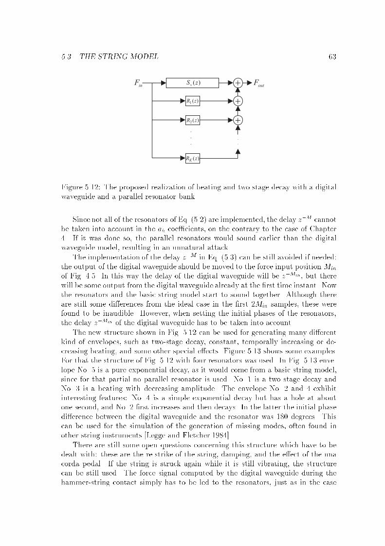
5.3. THE STRING MODEL 63

Figure 5.12: The proposed realization of beating and two-stage decay with a digitalwaveguide and a parallel resonator bank.

Since not all of the resonators of Eq. (5.2) are implemented, the delay z�M cannotbe taken into account in the ak coe�cients, on the contrary to the case of Chapter4. If it was done so, the parallel resonators would sound earlier than the digitalwaveguide model, resulting in an unnatural attack.

The implementation of the delay z�M in Eq. (5.3) can be still avoided if needed:the output of the digital waveguide should be moved to the force input position Min

of Fig. 4.5. In this way the delay of the digital waveguide will be z�Min , but therewill be some output from the digital waveguide already at the �rst time instant. Nowthe resonators and the basic string model start to sound together. Although thereare still some di�erences from the ideal case in the �rst 2Min samples, these werefound to be inaudible. However, when setting the initial phases of the resonators,the delay z�Min of the digital waveguide has to be taken into account.

The new structure shown in Fig. 5.12 can be used for generating many di�erentkind of envelopes, such as two-stage decay, constant, temporally increasing or de-creasing beating, and some other special e�ects. Figure 5.13 shows some examples.For that the structure of Fig. 5.12 with four resonators was used. In Fig. 5.13 enve-lope No. 5 is a pure exponential decay, as it would come from a basic string model,since for that partial no parallel resonator is used. No. 1 is a two stage decay andNo. 3 is a beating with decreasing amplitude. The envelope No. 2 and 4 exhibitinteresting features: No. 4 is a simple exponential decay but has a hole at aboutone second, and No. 2 �rst increases and then decays. In the latter the initial phasedi�erence between the digital waveguide and the resonator was 180 degrees. Thiscan be used for the simulation of the generation of missing modes, often found inother string instruments [Legge and Fletcher 1984].

There are still some open questions concerning this structure which have to bedealt with: these are the re-strike of the string, damping, and the e�ect of the unacorda pedal. If the string is struck again while it is still vibrating, the structurecan be still used. The force signal computed by the digital waveguide during thehammer-string contact simply has to be led to the resonators, just as in the case

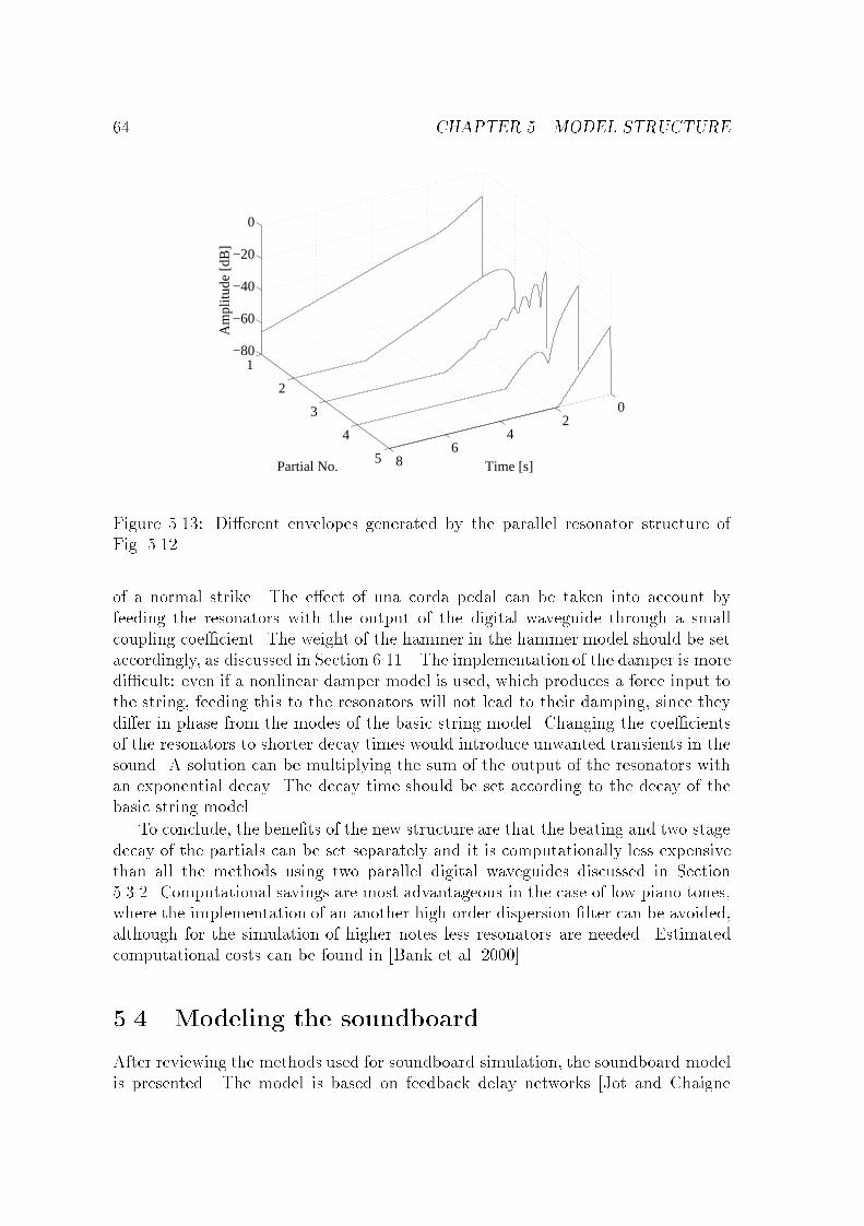
64 CHAPTER 5. MODEL STRUCTURE

02

46

8

1

2

3

4

5

−80

−60

−40

−20

0

Time [s]Partial No.

Am

plitu

de [d

B]

Figure 5.13: Di�erent envelopes generated by the parallel resonator structure ofFig. 5.12

of a normal strike. The e�ect of una corda pedal can be taken into account byfeeding the resonators with the output of the digital waveguide through a smallcoupling coe�cient. The weight of the hammer in the hammer model should be setaccordingly, as discussed in Section 6.11.. The implementation of the damper is moredi�cult: even if a nonlinear damper model is used, which produces a force input tothe string, feeding this to the resonators will not lead to their damping, since theydi�er in phase from the modes of the basic string model. Changing the coe�cientsof the resonators to shorter decay times would introduce unwanted transients in thesound. A solution can be multiplying the sum of the output of the resonators withan exponential decay. The decay time should be set according to the decay of thebasic string model.

To conclude, the bene�ts of the new structure are that the beating and two-stagedecay of the partials can be set separately and it is computationally less expensivethan all the methods using two parallel digital waveguides discussed in Section5.3.2. Computational savings are most advantageous in the case of low piano tones,where the implementation of an another high-order dispersion �lter can be avoided,although for the simulation of higher notes less resonators are needed. Estimatedcomputational costs can be found in [Bank et al. 2000].

5.4 Modeling the soundboard

After reviewing the methods used for soundboard simulation, the soundboard modelis presented. The model is based on feedback delay networks [Jot and Chaigne

5.4. MODELING THE SOUNDBOARD 65

1991]. The principles of feedback delay networks are also outlined. A new methodfor modeling the attack noise of the piano is proposed.

5.4.1 Earlier work on soundboard modeling

There are several di�erent approaches in the literature, concerning the simulation ofthe soundboard. The computationally most e�cient one is the commuted piano ofSmith and Van Duyne [1995]; Van Duyne and Smith [1995]. It is based on commutedsynthesis [Karjalainen and Välimäki 1993; Smith 1993], where the soundboard �lteris commuted with the digital waveguide and the hammer model. For this, the wholesystem has to be linear, hence the hammer model as well. The advantage of themethod is that the soundboard model does not have to be implemented as a highorder �lter, but as a wavetable, whose content is simply played to the string. Nodoubt, this is the computationally most e�cient soundboard modeling techniqueso far. However, it is a serious drawback that it cannot be used with a nonlinearhammer model (see Section 5.2.1).

The other end of the scale is the �nite di�erence soundboard model presented in[Giordano 1997]. It is physically meaningful and allows the simulation of di�erentfeatures of the soundboard, such as the e�ect of ribs. However, the solution of thetwo dimensional �nite di�erence equation takes a long computational time. There-fore, the �nite di�erence technique can be considered an analytical tool, and not asoundboard model candidate for sound synthesis.

A simple and e�cient piano soundboard model was presented in [Garnett 1987].The strings were modeled by digital waveguides, connected to the same termination.The soundboard was simulated by connecting six additional digital waveguides tothis common termination. Each of these interconnected waveguides contained alowpass �lter with a large damping factor. An advantage of the technique is thatit can provide high modal density for low computational cost. The disadvantageis that it simulates a general soundboard, modeling of the soundboard of a speci�cpiano is quite di�cult with this method.

A similar approach, suggested, e.g., in [Rocchesso and Smith 1997], is based onfeedback delay networks. Although this approach has not been used for modeling thesoundboard of the piano, but rather for room response simulation. The principlesof the feedback delay networks are outlined in the next section.

5.4.2 Feedback delay networks

Feedback delay networks can be considered the generalization of the state spacerepresentation of a discrete-time linear system [Rocchesso and Smith 1997]. Here,the elementary unit delays z�1 are replaced with delay lines of arbitrary length z�mk .The equations in the z domain are:

s(z) = D(z) (As(z) + bx(z))

y(z) = cT s(z) + dx(z) (5.4)

66 CHAPTER 5. MODEL STRUCTURE

where x(z) and y(z) are the input and output signals, s(z) is the state vector, D(z)is the diagonal delay matrixDkk = z�mk , and A is the feedback matrix. In Eq. (5.4)b is the input coe�cient vector, c is the output coe�cient vector, and d is the outputcoe�cient.

It can be shown that the technique used in [Garnett 1987], i.e., connecting digitalwaveguides to the same termination, is a special case of feedback delay networks[Rocchesso and Smith 1997].

An important issue is the stability of the system. The feedback delay network isstable when the corresponding state-space representation with z�1 = z�mk for eachdelay element is stable [Rocchesso and Smith 1997]. It was proven in [Rocchessoand Smith 1997] that as long as kAkn decays exponentially with n, the stabilityis assured. A straightforward approach for controlling the properties of the systemis making a lossless prototype and then introducing losses to the system [Jot andChaigne 1991; Rocchesso and Smith 1997]. For such a prototype, we need that allthe poles lie on the unit circle. This can be assured when the feedback matrix Ais unitary [see, e.g., Jot and Chaigne 1991; Rocchesso and Smith 1997]. Since wegenerally deal with systems with real coe�cients, the equivalent constraint is theorthogonality (A�1 = AT ) of the feedback matrix.

When the size of A is su�ciently large (about 12 rows and columns) and thetotal delay length is at least 1 second, the impulse response of the lossless prototypecan be compared to a pseudo-random noise generator [Jot 1992].

A new class of feedback delay networks was presented in [Rocchesso and Smith1997]. By choosing the feedback matrix to be circular, the distribution of eigenvaluesis easily controlled. The eigenvalues of the system and the �rst row of the circularfeedback matrixA are related through the Discrete Fourier Transform. Losslessnesscan be achieved by choosing eigenvalues of unit length, and calculating the feedbackmatrix by means of Inverse Discrete Fourier Transform.

Losses are introduced to the system by connecting �lters Hk(z) to the output ofthe delay lines [Jot and Chaigne 1991; Rocchesso and Smith 1997], that is, substitut-ing z�mk with z�mkHk(z) in the delay matrix D. Then, to maintain �at magnituderesponse, a tone corrector �lter has to be used in series to the feedback delay network[Jot and Chaigne 1991; Jot 1992].

5.4.3 The soundboard model

Feedback delay networks have been successfully used for room reverberation sim-ulation. This is because the late part of the impulse response of rooms can beconsidered as a nonstationary Gaussian process with a time-variant power spectraldensity. By properly choosing the feedback matrix A and the loss �lters Hk(z),similar output arises from the feedback delay network [Jot and Chaigne 1991]. Theunderlying metaphor and the connections of the response of a rectangular room andthe feedback delay network are discussed in [Rocchesso 1995].

The use of feedback delay networks for simulating the body of an instrumentwas suggested in [Rocchesso and Smith 1997]. This is motivated by the fact that

5.4. MODELING THE SOUNDBOARD 67

the exact position and height of resonances are perceptually insigni�cant. As longas the modal density and the decay times are close to the original one, the soundwill be similar. In reality, when listening to the impulse response of the soundboard,it sounds like a colored, decaying noise.

However, for soundboard modeling other considerations are needed than thosefor the room response simulation. The density of the pulses in the output of feed-back delay network is rather small in the beginning of the impulse response. Thiswell coincides with the behavior of real rooms, where the late reverberation slowlybuilds up. These early pulses in the response of the feedback delay network can beconsidered as the early re�ections in the room response. The colorless reverberationcan be ensured by using delay lines of comparable length [Rocchesso and Smith1997].

On the contrary, the impulse response of the piano soundboard does not showthis feature. It is rather a sum of damping modes, the rise in the attack cannotbe observed. If the soundboard is simulated with a delay line lengths of more thantwo or three hundred samples, the resulted sound will be rather cello-like, since thesharp attack of the piano sound disappears. Therefore, we need energy in the earlyregion of the impulse response as well. This can be done by applying short delaylines together with the long ones. The author has successfully used an eight delayline feedback delay network with gradually increasing delay lengths (37, 87, 181,271, 359, 492, 687, 721) for soundboard simulation. These are relative primes, inorder to avoid harmonic structure. For the losses, one-pole �lters were used in seriesto the delay lines. The parameters of the model are given in Section 6.5.

The feedback delay network model was found to be a good approximation ofthe soundboard impulse response. The main bene�t of such a structure againsttraditional FIR or IIR �lters comes from the e�cient implementation of the delaylines. This way, very high modal density can be obtained with relatively smallnumber of operations. The drawback is that the resonances cannot be controlledseparately. Consequently, this method is not capable to reproduce the exact copyof a real soundboard impulse response, but it is good enough to capture its mainfeatures.

From this point of view, its relation to general IIR �lters is similar to that of thedigital waveguide to the resonator bank. In IIR �lters the computational complexitydepends on the number of realized peaks in the transfer function. On the contrary,in feedback delay networks it comes from the accuracy of the approximation. Inother words, the feedback delay network is capable to simulate many modes for lowcomputational cost, but their place and height cannot be precisely controlled.

If the soundboard is simulated by the feedback delay network only, more naturalresult occurs, when the tone corrector �lter of [Jot and Chaigne 1991; Jot 1992] is notused. A better approximation has been obtained by whitening the impulse responsewith the tone corrector [Jot and Chaigne 1991; Jot 1992], and then �ltering with ashaping �lter whose magnitude response is similar to that of the real soundboard.The author has used a 100 tap FIR �lter with good results. The advantage ofthe FIR �lter that it can be easily designed by means of Inverse Discrete Fourier

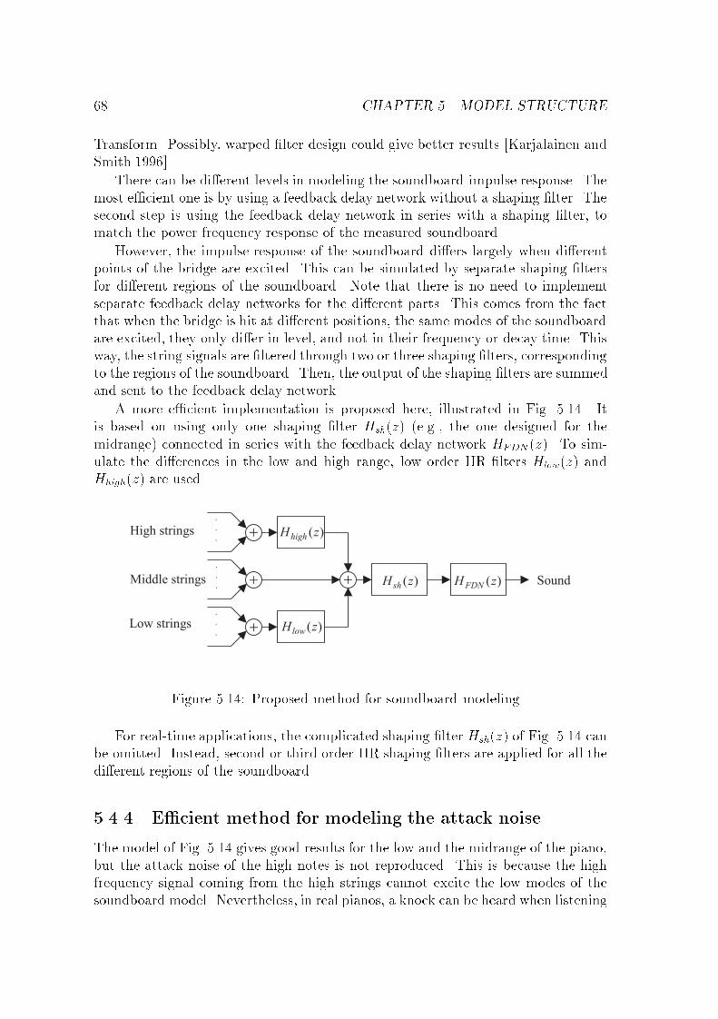
68 CHAPTER 5. MODEL STRUCTURE

Transform. Possibly, warped �lter design could give better results [Karjalainen andSmith 1996].

There can be di�erent levels in modeling the soundboard impulse response. Themost e�cient one is by using a feedback delay network without a shaping �lter. Thesecond step is using the feedback delay network in series with a shaping �lter, tomatch the power frequency response of the measured soundboard.

However, the impulse response of the soundboard di�ers largely when di�erentpoints of the bridge are excited. This can be simulated by separate shaping �ltersfor di�erent regions of the soundboard. Note that there is no need to implementseparate feedback delay networks for the di�erent parts. This comes from the factthat when the bridge is hit at di�erent positions, the same modes of the soundboardare excited, they only di�er in level, and not in their frequency or decay time. Thisway, the string signals are �ltered through two or three shaping �lters, correspondingto the regions of the soundboard. Then, the output of the shaping �lters are summedand sent to the feedback delay network.

A more e�cient implementation is proposed here, illustrated in Fig. 5.14. Itis based on using only one shaping �lter Hsh(z) (e.g., the one designed for themidrange) connected in series with the feedback delay network HFDN (z). To sim-ulate the di�erences in the low and high range, low order IIR �lters Hlow(z) andHhigh(z) are used.

Figure 5.14: Proposed method for soundboard modeling.

For real-time applications, the complicated shaping �lter Hsh(z) of Fig. 5.14 canbe omitted. Instead, second or third order IIR shaping �lters are applied for all thedi�erent regions of the soundboard.

5.4.4 E�cient method for modeling the attack noise

The model of Fig. 5.14 gives good results for the low and the midrange of the piano,but the attack noise of the high notes is not reproduced. This is because the highfrequency signal coming from the high strings cannot excite the low modes of thesoundboard model. Nevertheless, in real pianos, a knock can be heard when listening

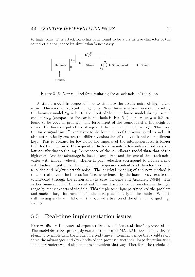
5.5. REAL-TIME IMPLEMENTATION ISSUES 69

to high tones. This attack noise has been found to be a distinctive character of thesound of pianos, hence its simulation is necessary.

Figure 5.15: New method for simulating the attack noise of the piano.

A simple model is proposed here to simulate the attack noise of high pianotones. The idea is displayed in Fig. 5.15. Now the interaction force calculated bythe hammer model FH is led to the input of the soundboard model through a realcoe�cient g (compare to the earlier methods in Fig. 5.1). The value g = 0:2 wasfound to be good in practice. The force input of the soundboard is the weightedsum of the force output of the string and the hammer, i.e., FS + gFH . This way,the force signal can e�ciently excite the low modes of the soundboard as well. Italso automatically ensures the di�erent coloration of the attack noise for di�erentkeys. This is because for low notes the impulse of the interaction force is longerthan for the high ones. Consequently, the force signals of low notes introduce morelowpass �ltering to the impulse response of the soundboard model than that of thehigh ones. Another advantage is that the amplitude and the tone of the attack noisevaries with impact velocity. Higher impact velocities correspond to a force signalwith higher amplitude and stronger high frequency content, and therefore result ina louder and brighter attack noise. The physical meaning of the new method isthat in real pianos the interaction force experienced by the hammer can excite thesoundboard through the action and the case [Chaigne and Askenfelt 1994b]. Theearlier piano model of the present author was described to be too clean in the highrange by many experts of the �eld. This simple technique partly solved the problemand made a large improvement in the perceptual quality of the model. What isstill missing is the simulation of the coupled vibration of the other undamped highstrings.

5.5 Real-time implementation issues

Here we discuss the practical aspects related to e�cient real-time implementation.The model described previously exists in the form of MATLAB code. The author isplanning to implement the model in a real-time environment, since that could reallyshow the advantages and drawbacks of the proposed methods. Experimenting withsome parameters would also be more convenient that way. Therefore, the techniques

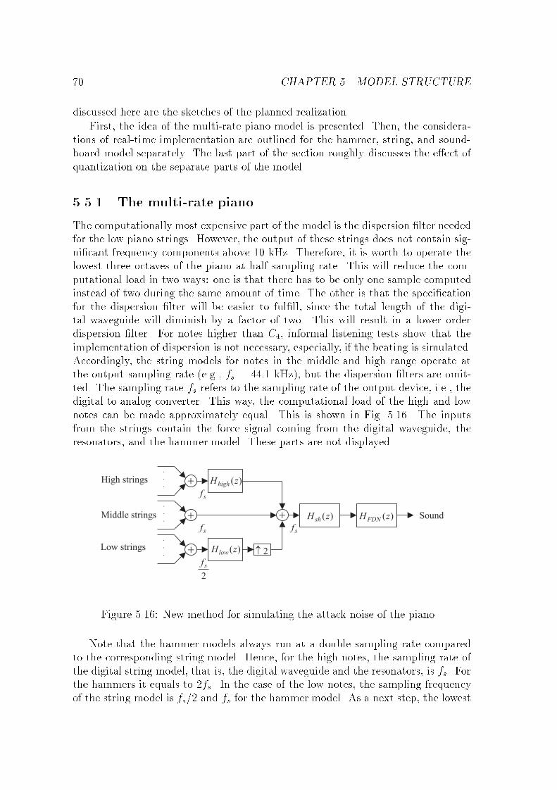
70 CHAPTER 5. MODEL STRUCTURE

discussed here are the sketches of the planned realization.

First, the idea of the multi-rate piano model is presented. Then, the considera-tions of real-time implementation are outlined for the hammer, string, and sound-board model separately. The last part of the section roughly discusses the e�ect ofquantization on the separate parts of the model.

5.5.1 The multi-rate piano

The computationally most expensive part of the model is the dispersion �lter neededfor the low piano strings. However, the output of these strings does not contain sig-ni�cant frequency components above 10 kHz. Therefore, it is worth to operate thelowest three octaves of the piano at half sampling rate. This will reduce the com-putational load in two ways: one is that there has to be only one sample computedinstead of two during the same amount of time. The other is that the speci�cationfor the dispersion �lter will be easier to ful�ll, since the total length of the digi-tal waveguide will diminish by a factor of two. This will result in a lower orderdispersion �lter. For notes higher than C4, informal listening tests show that theimplementation of dispersion is not necessary, especially, if the beating is simulated.Accordingly, the string models for notes in the middle and high range operate atthe output sampling rate (e.g., fs = 44:1 kHz), but the dispersion �lters are omit-ted. The sampling rate fs refers to the sampling rate of the output device, i.e., thedigital-to-analog converter. This way, the computational load of the high and lownotes can be made approximately equal. This is shown in Fig. 5.16. The inputsfrom the strings contain the force signal coming from the digital waveguide, theresonators, and the hammer model. These parts are not displayed.

Figure 5.16: New method for simulating the attack noise of the piano.

Note that the hammer models always run at a double sampling rate comparedto the corresponding string model. Hence, for the high notes, the sampling rate ofthe digital string model, that is, the digital waveguide and the resonators, is fs. Forthe hammers it equals to 2fs. In the case of the low notes, the sampling frequencyof the string model is fs=2 and fs for the hammer model. As a next step, the lowest

5.5. REAL-TIME IMPLEMENTATION ISSUES 71

octave of the piano can be operated at the fourth of the normal sampling rate fs=4,but that could lead to some degradation in sound quality.

The shaping �lters are operated at the same sampling rate as the strings con-nected to them. Then, the signal of the low register with sampling rate fs=2 isupsampled. Probably a 10th order FIR �lter will be appropriate for this purpose.After upsampling, the output signal of the low strings is added to that of the highones and fed to the shaping �lter and the feedback delay network.

5.5.2 Hammer and dampers

The implementation of the hammer model is quite straightforward. This is be-cause it can be considered a linear �lter connected in series with an instantaneousnonlinearity.

The only problem here is the realization of the F (�y) = K(�y)p function (seeFig. 5.5). One way is to use a lookup table with the values of (�y)p for �y valuesthat normally occur and for about ten p values between 2 and 3. The not stored�y values can be determined by means of linear interpolation.

A simpler solution, also proposed in [Borin and De Poli 1996], can be to ap-proximate K(�y)p with K2(�y)

2 +K3(�y)3. Alternatively, when determining the

parameters of the hammer model, this polynomial form could be used for optimiza-tion (see Section 6.1.1). An advantage of this approach is that no lookup-table isneeded. The interpolation between di�erent felt characteristics is straightforward,because the linear interpolation of K2 and K3 parameters give meaningful results.Note that in the case of a force model K(�y) it is not obvious how to interpolatebetween force characteristics of di�erent p values.

The fact, that the hammer runs at the double sampling frequency, does not leadto any complication in the implementation. From outside, the double sampling rateis not visible. It only means that the same kind of operations are executed twice inthe program code.

The dampers can be realized as one-pole �lters connected to the digital waveguidein series. The implementation of a nonlinear damper needs similar considerationsas the hammer model. The problem is the lack of data about real damper behavior.However, a real-time implementation could be useful in this sense, since the smallnumber of parameters of the damper model could be tuned just by listening to theresult.

5.5.3 String model

The e�ciency of the digital waveguide lies in the delay lines: they can be imple-mented as circular bu�ers. By commuting the �1 signs in Fig. 4.5, the �gure can beredrawn with two delay lines, without any sign change in the feedback loop [Smithand Van Duyne 1995]. This is similar to the case when the variables of the waveg-uide are force waves. The di�erence is up to a constant factor Z0. From a practicalpoint of view it is worth to use force signals in the delay lines instead of the velocity.

72 CHAPTER 5. MODEL STRUCTURE

This is because both the input and the output of the digital waveguide are forces.By doing so, the connections of the hammer model and the digital waveguide haveto be changed.

Now that there is no sign change in the delay lines, the whole digital waveguidecan be implemented as one circular bu�er with four pointers. Four pointers areneeded to compute the input of the hammer (see Eq. 5.1) and two of them are usedfor inserting the force input to the digital waveguide. The output of the digitalwaveguide is taken from the position y+(n;Min). Then, this cell is overwritten bythe �ltered version of the output signal. This realizes the re�ection �lter Hrv(z).After that, all the four pointers are shifted by one step.

The implementation of the resonator bank is rather straightforward, since itconsists of parallel second order sections.

5.5.4 The soundboard

The soundboard is implemented as a feedback delay network with correction andshaping �lters (see Fig. 5.14).

The delay lines of the feedback delay network are implemented as simple circularbu�ers. The most time-consuming operation of the feedback delay network is thematrix multiplication (see Eq. 5.4). Nevertheless, by the careful choice of the feed-back matrix A, the matrix multiplication can be eliminated [Rocchesso and Smith1997]. For example, in the case of the circular feedback matrix presented in Section6.5.1, all the output signals of the delay lines after the loss �lter are summed, mul-tiplied by �1=4 and fed into the input of all the delay lines. This corresponds tothe �1=4 elements of the feedback matrix A. The consecutive delay lines are alsoconnected with gain factors of 1. The latter implements the elements 1� 1=4 in thefeedback matrix.

5.5.5 Finite wordlength e�ects

For practical implementation, it is interesting to examine how sensitive the di�erentparts of the system are for roundo� errors. The problem with the hammer model liesin the digital integrators, since there a very small value is added to the past output.Some of the problems can be avoided by rescaling the signal levels in Fig. 5.5, i.e.,using nonphysical variables. However, their realization seems to be problematic in16-bit arithmetic.

The re�ection �lter of the digital waveguide is sensitive to quantization. Itsmagnitude response is close to 1, which means very small coe�cients. Also the dis-persion �lter can have large di�erence in the values of its coe�cients, if implementedin direct form. Therefore, to avoid instabilities, the re�ection �lter should be splitinto second order sections. If the quantization of the architecture is very rude, eventhe use of an FIR loss �lter should be considered. The second order resonators of theresonator bank can also face with stability problems, since the implemented quality

5.6. CONCLUSION 73

factor values are very large. Interpolated low frequency resonators could overcomethis problem [Välimäki and Tolonen 1998].

On the contrary, the soundboard model is quite robust against quantizationerrors. This is because there the magnitude of the loss �lters is not as close to unityas that of the string model. The shaping �lter is an FIR �lter, which is stable byprinciple.

To sum up, it seems that a 16-bit �x point arithmetic is not enough for the pianomodel. At least 24-bit �x point arithmetic should be used. The best solution wouldbe the use of a �oating point architecture. Then the physical units of the variablescould be directly used, i.e., they would not need any rescaling.

5.6 Conclusion

We discussed the structure of the piano model. After outlining the general structureof the piano, the hammer and damper models were presented. The discontinuityproblem of the string was analyzed and methods were suggested for taking in theinteraction force to the digital waveguide in a correct way. A new multi-rate hammermodel was presented, which is stable even for extremely high impact velocities. Theadvantage of this method compared to those of the literature lies in its simplicity.The same structure can also be used for the simulation of the e�ect of dampers, albeitthe calibration of such a damper model has not been solved yet. A novel resonatorbank based structure was presented for the simulation of beating and two-stagedecay. Although it simulates the harmonics separately, it responds to the variationof the interaction force automatically. The soundboard is simulated by a feedbackdelay network, a technique which has been found very successful in room responsemodeling. It can be viewed as a statistical model of the impulse response, sinceonly the general properties of the soundboard are matched. A simple technique formodeling the attack sound of the piano was presented. The last part of the chapterdealt with practical implementation issues. There, a multi-rate piano model waspresented, which balances the computational load of the high and low strings of themodel.

74 CHAPTER 5. MODEL STRUCTURE

Chapter 6

Model calibration

In the previous chapter the structure of the piano model was presented. Here wediscuss the calibration of the di�erent parts of the model. This is the inverse op-eration of the simulation, since in simulation the inputs are the model parametersand the output is the audible sound. Here the case is the contrary: we wish to �ndparameters for our model which give the most similar sound output to the sound ofthe real piano.

Theoretically, the easiest approach would be a nonlinear optimization processfor all the parameters of the model. It is the easiest from the point of view of thescientist, and not of the computer, of course. This optimization could be done byapplying genetic algorithms or neural networks for searching in the parameter spaceand maximizing a �tness function between the original and the synthesized signal.However, this would lead to instabilities in the parameter estimation, not to mentionthe need for a lot of computational power. Finding an appropriate �tness functioncould also be problematic.

The basic idea of this chapter is to keep the parameter estimation as simple aspossible, with respect to the necessary computations. The building blocks of theprocedures should be well known and easily realizable operations. The calibrationprocess should be straightforward, without any feedback from the output of themodel, to avoid any instabilities. This kind of approach needs more analytical work,since the behavior of the model structure should be well understood.

Two new �lter design algorithms are presented for the digital waveguide, one forthe general case and another for the one-pole loop �lter. The idea of both methods isto minimize the error of the resulting decay times, and not the magnitude response ofthe �lter. An advantage of these techniques is that the stability of the �lters can beeasily assured. In Section 5.3.3, a new technique was proposed for the simulation ofbeating and two-stage decay. A novel method had to be developed for the calibrationof this structure, which was found to be robust and reliable for all kind of pianosounds.

75

76 CHAPTER 6. MODEL CALIBRATION

6.1 Parameters of hammer and damper models

The parameters for the hammer model were taken from the literature, because of thelack of time. Nevertheless, a simple method for calibrating the hammer is proposed.The calibration of the linear damper model is similar to that of the digital waveguide,which is discussed in Section 6.2.

6.1.1 Calibration of the hammer

For the implemented piano model, the parameters of [Chaigne and Askenfelt 1994a]were used. The parameters of the three hammers measured in [Chaigne and Asken-felt 1994a] were interpolated for other notes. The hammer mass parameter of themodel was set in a way that the ratio of hammer and string mass was the same asfor the real piano. This means that the mass of a hammer which hits a triplet, hasto be divided by three, since in the model it is connected to one digital waveguideonly. For the same hammer, if the una corda pedal is depressed, the hammer massin the model will be the half of the real hammer mass.

However, there were only three hammers measured in [Chaigne and Askenfelt1994a], which obviously does not cover the entire keyboard. It would be also bene�-cial to make hammer measurements on old pianofortes, since their simulation couldbe even more interesting than the modern ones.

A method proposed here for estimation of hammer parameters is based on thework of [Boutillon 1988]. A miniature accelerometer is attached to the measuredhammer. Then, the key is hit several times at di�erent dynamic levels. The accel-eration signal is recorded for analysis. The impact velocities of the hammer can becomputed by integrating the acceleration signal. Then, a digital waveguide modelwith the proposed hammer model is run, and the acceleration of the hammer is com-puted. By using standard optimization algorithms, the di�erence of the two signalscan be minimized with respect to the hammer parameters. The initial guesses forthe optimization can be obtained from analytic expressions of the hammer behavior(see Section 2.1.2 for references). The hammer mass is computed by subtracting themass of the accelerometer from the outcome of the optimization. An advantage ofthe method is that the piano action does not have to be disassembled, and it doesnot make any harm in the hammer felt.

6.1.2 Calibration of the dampers

The calibration of the damper is similar to that of [Erkut et al. 2000], and it isbased on recorded piano tones. The analyzed signal can be sound pressure or theacceleration of the bridge. The procedure is as follows: �rst, the beginning of thedamping has to be determined. This was done manually, but it could be madeautomatic by looking for a jump in the time derivate of the amplitude envelope.This time instant will be the beginning of the analysis signal. The end is wherethe amplitude of the partials falls under the noise level. After determining the

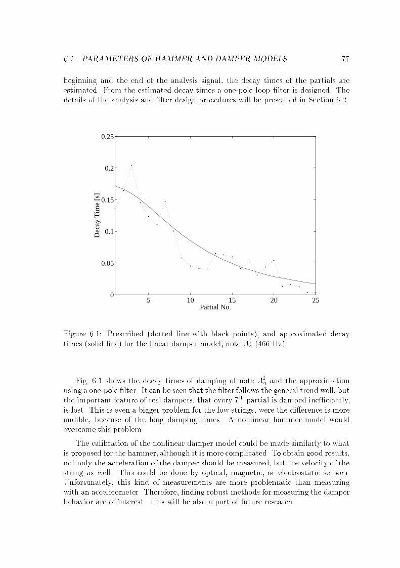
6.1. PARAMETERS OF HAMMER AND DAMPER MODELS 77

beginning and the end of the analysis signal, the decay times of the partials areestimated. From the estimated decay times a one-pole loop �lter is designed. Thedetails of the analysis and �lter design procedures will be presented in Section 6.2.

5 10 15 20 250

0.05

0.1

0.15

0.2

0.25

Partial No.

Dec

ay T

ime

[s]

Figure 6.1: Prescribed (dotted line with black points), and approximated decaytimes (solid line) for the linear damper model, note A]

4 (466 Hz).

Fig. 6.1 shows the decay times of damping of note A]4 and the approximation

using a one-pole �lter. It can be seen that the �lter follows the general trend well, butthe important feature of real dampers, that every 7th partial is damped ine�ciently,is lost. This is even a bigger problem for the low strings, were the di�erence is moreaudible, because of the long damping times. A nonlinear hammer model wouldovercome this problem.

The calibration of the nonlinear damper model could be made similarly to whatis proposed for the hammer, although it is more complicated. To obtain good results,not only the acceleration of the damper should be measured, but the velocity of thestring as well. This could be done by optical, magnetic, or electrostatic sensors.Unfortunately, this kind of measurements are more problematic than measuringwith an accelerometer. Therefore, �nding robust methods for measuring the damperbehavior are of interest. This will be also a part of future research.

78 CHAPTER 6. MODEL CALIBRATION

6.2 Parameter estimation for the string model

Since the model used for simulating the string behavior consists of two di�erentparts, namely, the digital waveguide and the resonator bank, the calibration ofthese needs di�erent considerations. Accordingly, the description of the string cali-bration is split to three sections. The �rst two discuss the calibration of the digitalwaveguide, namely, signal estimation and �lter design, and the third concentrateson the calibration of the resonator bank.

The calibration of the digital waveguide consists of designing the re�ection �lterHrv(z) and setting the length of the digital waveguide M in Fig. 4.5. One approachcould be the impedance measurement of the bridge and the analytic derivation ofstring losses and vibration. This could give an insight to the physical behavior ofthe string-soundboard system. The separation of the e�ects of the string and thetermination could be helpful in determining the parameters of a model displayedon Fig. 5.10 or 5.11. Smith [1983] computed the speci�cation for the re�ection�lter Hrv(z) by means of linear prediction and by a system identi�cation method.However, these did not give a robust solution. A more straightforward approachtaken here, also suggested by Välimäki et al. [1996], is based on the measurement ofpartial envelopes. The loss and dispersion �lters can be designed from the frequenciesand the decay times of the partials. This way, the e�ects introduced by the stringand the termination cannot be separated, but it is not needed for a single-stringdigital waveguide model. The interest is now only on designing a digital waveguidewhose behavior is similar to the measured string.

6.2.1 Overview of signal estimation methods

For the analysis of the partials, basically two types of methods are used in the liter-ature. One is based on the Short Time Fourier Transform [Allen and Rabiner 1977].The signal is �rst multiplied by a window function with a length corresponding tointeger number multiples of the pitch period. Then the DFT of the windowed datais computed. As this is done for several time instants, the result is the temporalevolution of the short time spectrum. By �nding and following the peaks of thesespectra, the frequencies and the decay times of the partials can be calculated. Themethod has been described in [Välimäki et al. 1996].

The other approach, also taken here, uses heterodyne �ltering [Moorer 1977].The observed partial is brought to around zero in the frequency domain by multi-plying the signal with a complex exponential corresponding to that frequency. Thefrequency components of other partials are suppressed by lowpass �ltering. Theamplitude of the partial is calculated by taking the absolute value of the lowpass�ltered signal [Välimäki and Tolonen 1998; Ding and Qian 1997]. The signal is ex-amined only at the partial frequencies, and this speeds up the analysis procedurecompared to the DFT based approach.

6.2. PARAMETER ESTIMATION FOR THE STRING MODEL 79

6.2.2 Heterodyne �ltering for signal estimation

Both the sound pressure and bridge acceleration of several piano tones were recordedfor analysis in this study. The bridge acceleration signals were found to be moreuseful than the sound pressure, since they contained stronger high harmonics. Thisis because the pressure signal is rather proportional to the bridge velocity, i.e., itsspectrum falls at a rate of 20 dB/decade compared to acceleration. The frequenciesand decay times of the partials are the same for the pressure and acceleration signals.Their amplitudes di�er but the initial amplitudes are irrelevant in the �lter design.

The heterodyne technique was chosen for the analysis of the measured signal,mostly because of its computational simplicity. The steps of the algorithm areillustrated in Fig. 6.2. The fundamental frequency of the tone can be calculated bysome pitch estimation methods, for example based on the autocorrelation function[Rabiner 1977; Välimäki et al. 1996], or by �nding peaks in the DFT of the signal.This is not needed here, because the fundamental frequency of the analyzed note isapproximately known, since it comes from which key of the piano was depressed.

The analyzed signal x(n) is multiplied by a complex exponential e�j#1n corre-sponding to the fundamental angular frequency estimate #1. Then the resultedcomplex signal is lowpass �ltered. There is a tradeo� between the time domainand frequency domain resolution of the analysis: if the lowpass �lter Hlpf has alow cut-o� frequency, the envelopes (especially in the attack part) will be some-what smeared, but it will suppress the measurement noise appropriately. On thecontrary, high cut-o� frequency leads to more noise, making the analysis procedureuncertain. The cuto� frequency of the �lter obviously has to be below the fundamen-tal frequency of the tone. Here, a fourth-order Butterworth �lter was used, designedby the MATLAB butter command. To avoid phase distortion, the data was �lteredin both forward and backward directions, by using the MATLAB filtfilt proce-dure [MAT 1996]. In this way, the resulted �lter had an order of eight. The cuto�frequency was set to half of the fundamental for the very low notes and to one fourthfor the others.

The amplitude envelope of the partial is computed by simply taking the absolutevalue of the �ltered complex signal. Note that this does not give the amplitude ofthe sinusoidal representation, but the amplitude of the complex exponential. Toobtain the amplitude of the corresponding sinusoid, the value should be multipliedby two. However, we are not interested here in the amplitudes, but the decay times.But before computing those, the time-span of valid data should be found. For thebeginning of the note, a good estimate is the time instant with maximal amplitude,since the piano sound is decaying by nature. Finding the end is somewhat morecomplicated. If the measured data is long enough, its very last part consists ofmeasurement noise only, whose level is then computed. The note is assumed to beterminated when its level falls below a certain limit, which was set to 10 dB abovethe measurement noise. The decay times �k are estimated by taking the logarithm ofthe amplitude envelope and applying linear regression to that, similarly to [Välimäkiet al. 1996]. The slope of the �tted line determines the decay time of the partial.

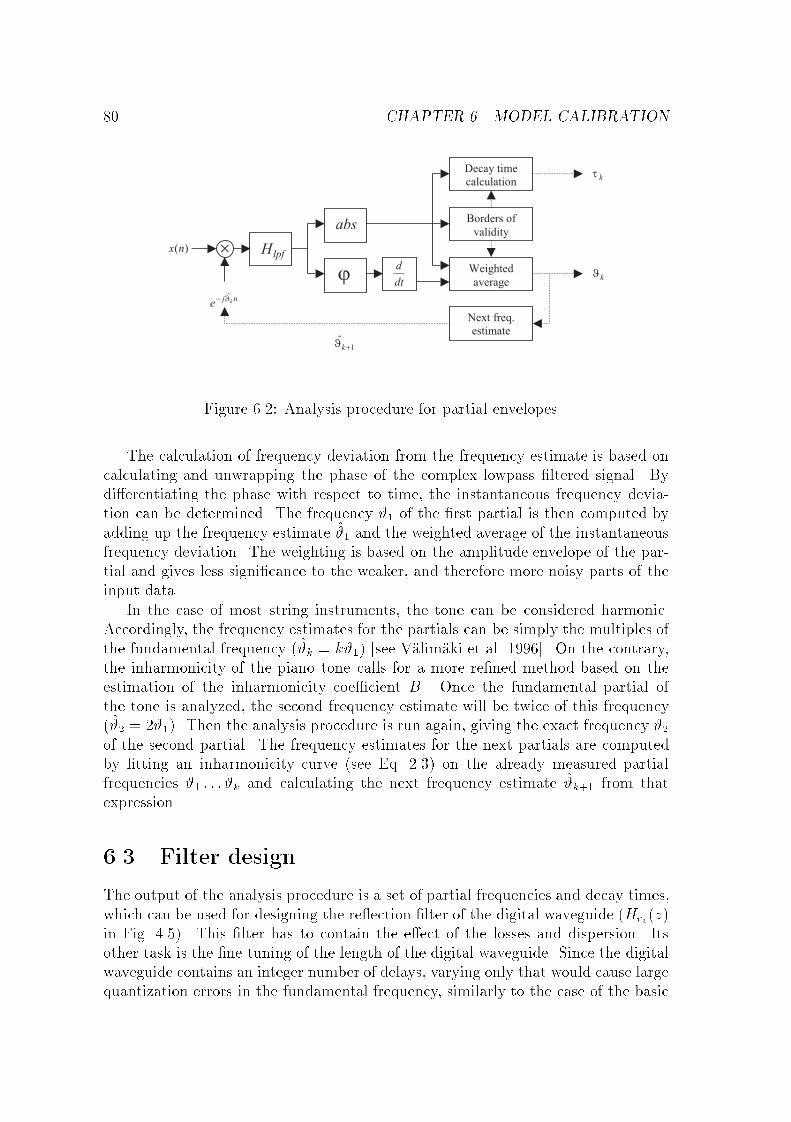
80 CHAPTER 6. MODEL CALIBRATION

Figure 6.2: Analysis procedure for partial envelopes.

The calculation of frequency deviation from the frequency estimate is based oncalculating and unwrapping the phase of the complex lowpass �ltered signal. Bydi�erentiating the phase with respect to time, the instantaneous frequency devia-tion can be determined. The frequency #1 of the �rst partial is then computed byadding up the frequency estimate #1 and the weighted average of the instantaneousfrequency deviation. The weighting is based on the amplitude envelope of the par-tial and gives less signi�cance to the weaker, and therefore more noisy parts of theinput data.

In the case of most string instruments, the tone can be considered harmonic.Accordingly, the frequency estimates for the partials can be simply the multiples ofthe fundamental frequency (#k = k#1) [see Välimäki et al. 1996]. On the contrary,the inharmonicity of the piano tone calls for a more re�ned method based on theestimation of the inharmonicity coe�cient B. Once the fundamental partial ofthe tone is analyzed, the second frequency estimate will be twice of this frequency(#2 = 2#1). Then the analysis procedure is run again, giving the exact frequency #2of the second partial. The frequency estimates for the next partials are computedby �tting an inharmonicity curve (see Eq. 2.3) on the already measured partialfrequencies #1 : : : #k and calculating the next frequency estimate #k+1 from thatexpression.

6.3 Filter design

The output of the analysis procedure is a set of partial frequencies and decay times,which can be used for designing the re�ection �lter of the digital waveguide (Hrv(z)in Fig. 4.5). This �lter has to contain the e�ect of the losses and dispersion. Itsother task is the �ne-tuning of the length of the digital waveguide. Since the digitalwaveguide contains an integer number of delays, varying only that would cause largequantization errors in the fundamental frequency, similarly to the case of the basic

6.3. FILTER DESIGN 81

Karplus-Strong algorithm [Karplus and Strong 1983; Ja�e and Smith 1983].The analysis data results in a complex speci�cation, which could be directly used

for �lter design. For this, one should be able to separate the phase and the amplitudeerror of the approximation, since for those di�erent constraints are needed. Thephase response of the re�ection �lter has to be very accurate at the fundamentalfrequency of the note. On the contrary, at other frequencies it is enough if it followsthe general trend of the prescription. If the shape of the phase delay is similar towhat is needed to simulate the inharmonicity, the sound output will be still piano-like, even if there are some inaccuracies. The decay times of the partials dependon the amplitude response of the �lter, as shown in Eq. (4.16). It follows from theequation, that the closer the amplitude response is to 1, the larger error will arise indecay times for the same amplitude di�erence. The amplitude response should neverbe larger than 1, since it would make the feedback loop unstable. Consequently, avery complicated �lter design algorithm would be needed, considering the di�erentkind of approximation errors, in order to give good results.

Smith [1983] reviews a number of sophisticated �lter design techniques, twoof them are also discussed in [Laroche and Jot 1992]. However, these methodssu�er from instabilities. The papers rather suggest the division of the �lter designprocedure to the loss �lter, dispersion �lter and fractional delay �lter parts [Ja�eand Smith 1983; Välimäki et al. 1996]. By using allpass �lters for simulating thedispersion and controlling the fundamental frequency of the note, the amplituderesponse of the re�ection �lter will depend only on the loss �lter, simplifying the�lter design procedure largely. The slight phase di�erence caused by the loss �ltercan be neglected when compared to the phase response of the dispersion �lter.

Note that dividing the �lter design into di�erent steps cannot give mathemati-cally optimal results, since the separate parts of the �lters have some constrains onthe �lter coe�cients, like being allpass for the dispersion �lter. Now the simplicityof the analysis will lead to computationally less e�cient implementation. It followsthat in the future it is of great interest to �nd a robust algorithm which could de-sign one complete re�ection �lter based on the previously mentioned amplitude andphase criteria.

6.3.1 Review of loss �lter design algorithms

The speci�cation for the loss �lter can be computed by using the inverse of Eq. (4.16):

gk = e�

1

f0�k (6.1)

where �k is the decay time of partial k, f0 is the fundamental frequency of the noteand gk is the desired amplitude value of the loss �lter at the angular frequency #kof partial k. Fitting a �lter to gk coe�cients is not trivial, even if the phase part ofthe transfer function is not considered. This is because of the previously mentionednature of the loop �lter: the error in the decay time is a nonlinear function ofthe amplitude error. The stability of the digital waveguide loop is also hard to

82 CHAPTER 6. MODEL CALIBRATION

handle. Unfortunately, there exists quite a small number of papers in the literatureconcerning this subject. The methods reviewed in [Smith 1983] were found to betoo complicated for practical implementation. The stability constraint of the digitalwaveguide jHrv(z)j < 1 cannot be incorporated in these methods either.

In [Välimäki et al. 1996; Välimäki and Tolonen 1998] the problem was solved byusing a one-pole �lter. The transfer function of such a �lter is:

H1p(z) = g1 + a1

1 + a1z�1(6.2)

where �a1 is the pole of the �lter and g refers to the DC gain. In [Välimäki etal. 1996; Välimäki and Tolonen 1998] such a �lter was found to be adequate forsimulating the acoustic guitar and other plucked string instruments. The DC gaing was set according to the decay time of the �rst partial (g = g1), or the averageof the �rst two or three gk coe�cients. The pole of the �lter was determined bycontinuously adjusting a1 and searching for the minimumof the analytical expressionof the approximation error. The error was computed in a least squares sense, byusing a weighting function putting more emphasis on slowly decaying partials. Ja�eand Smith [1983] also discussed the use of the one-pole �lter, but without the gainfactor, i.e., g = 1 in Eq. (6.2).

The advantage of using a one-pole �lter is that it is always of a lowpass characterfor a1 < 0. Since g is less than unity by the principle of calculating it, the waveguideloop will be always stable. As we discuss in the Appendix, such a simple constraintcan be found for the �rst-order FIR �lter as well. The problem of the technique of[Välimäki et al. 1996] comes from the separation of the g and a1 parameters, since�rst g is set and then a1 is optimized assuming g to be given. Nonlinear optimizationcan overcome this problem, as presented in [Erkut et al. 2000]. There the previouslymentioned procedure was used calculating the initial estimates for g and a1. Thena nonlinear optimization was carried out based on the amplitude envelope of thesynthesized and the original signal. This is motivated by the fact that the overalldecay time of the synthesized sound has a large perceptual signi�cance. On theother hand, the timbral evolution of the sound was not taken into account in thenonlinear optimization loop, still not leading to an optimal solution. However, it isa question, how precise the approximation must be. Listening tests show that thethreshold for recognizing di�erences in the overall decay time is rather high [Tolonenand Järveläinen 2000].

6.3.2 The transformation method: a novel loss �lter design

technique

The fact that the loss �lter has only one pole is also a hard constraint itself, sinceit restricts the sets of realizable decay times to a great extent. As we shall see, inthe case of the piano the dispersion �lter is computationally much more expensivethan the loss �lter. Hence, applying e.g., a fourth-order loss �lter instead of a �rst-order one would not increase the computational costs signi�cantly. A straightforward

6.3. FILTER DESIGN 83

solution for designing such a �lter is to use standard �lter design methods for gk witha weighting function, e.g., such as presented in [Välimäki et al. 1996]. Unfortunatelythis does not lead to useful results, since in most of the cases the amplitude responseof the resulted �lter goes above unity and the decay times calculated from thedesigned �lter are nothing similar to those of the speci�cation. This is because thedependence of the decay times on the �lter magnitude is highly nonlinear. Note thatweighting would give a solution to that only if this relation could be assumed linear.Until this time, no general and robust solution to the problem has been presentedin the literature.

The new approach taken here is based on a perceptually meaningful criterion.Rather than minimizing the amplitude error of the �lter, it optimizes the resultingdecay times. The error e� of the decay times used in the following derivationsis de�ned in the mean-square sense, but it could also be minimized according tominimax or absolute error criteria. Consequently, the results obtained here forleast-squares optimization are valid for the other criteria as well, although whenweights wk 6= 1 are used, some corrections are necessary. The squared decay timeerror is de�ned as :

e� =KXk=1

(�k � �k)2 (6.3)

where �k are the prescribed, and �k are the approximated decay times of partial k.K refers to the number of partials with which the �lter design is carried out. Bysubstituting the expression of decay times (see Eq. 4.16) and using the �rst-orderTaylor series approximation for the ln function (lnx � x� 1 for x � 1) one obtains:

e� =KXk=1

1

f0 ln gk� 1

f0 ln gk

!2

� 1

f20

KXk=1

1

1 � gk� 1

1 � gk

!2

(6.4)

where gk are the prescribed �lter magnitudes at the partial frequencies jvarthetakand gk = jHgk(e

j#k)j are the corresponding values of the approximation. Since thegk and gk values are close to 1, the approximation for the error is very accurate.

Based on Eq. (6.5) a transformed �lter Htr(z) is designed. This can be done byany least squares �lter design algorithm (e.g., invfreqz in MATLAB) by using atransformed speci�cation gk;tr. This minimizes the error:

eLS =KXk=1

wk

�Htr(e

j#k)� gk;tr�2; gk;tr =

1

1 � gk(6.5)

where #k refers to the frequency of partial k and wk is the corresponding weight,which is now equal to 1 for all k. The error eLS di�ers from the right hand side ofEq. (6.4) by a constant factor only, which means that if Eq. (6.5) has a minimum, sodo Eqs. (6.4) and (6.3). This implies that the deviation from the prescribed decaytimes is minimized. The loss �lter Hgk(z) can be computed from the transformed�lter Htr(z) by an inverse transformation:

Hgk(z) = 1� 1

Htr(z)(6.6)

84 CHAPTER 6. MODEL CALIBRATION

Minimizing the error of the decay times puts more emphasis on the lower, slowlydecaying partials than on the higher ones, since the same absolute di�erence willgive larger relative error for shorter decay times. The relative error

e�;rel =KXk=1

�k�k� 1

!2

(6.7)

can also be minimized by using the same procedure described above, but a weightingof wk = 1=� 2k or the corresponding wk = (1�gk)2 should be used in the least squares�lter design algorithm (see Eq. 6.5).

In practice, the approach of Eq. (6.3) was found to be more successful than ofEq. (6.7), since it automatically gives better approximation for the lower harmonicsthan for the higher ones, and it thus preserves the original decay time. Althoughsimply minimizing the error of the decay times gave good results, it would be stillinteresting to experiment with other weighting functions, based on some psychoa-coustic criteria on the audibility of decay time deviations of the partials. The audi-bility of the overall decay time deviations were studied in [Tolonen and Järveläinen2000]. Unfortunately, the research was conducted for the one-pole loop �lter case,and hence the results cannot be directly used for designing a weighting function.One interesting outcome of the study is that variations of 25 to 40 % in the overalldecay time are inaudible.

There is still one point which has to be considered: calculating the gk coe�cientsby Eq. (6.1) is precise only if the inharmonicity of the digital waveguide can beneglected, that is, the partial frequencies are multiples of the fundamental frequency(fk = kf0). In the case of the piano string model, when the inharmonicity issimulated by a dispersion �lter, the e�ective length of the digital waveguide will besmaller for the higher harmonics than for the lower ones. Consequently, componentsof high frequency will travel around the digital waveguide more times during thesame amount of time than in the harmonic case. This will result in more dampingthan desired. The audibility of the error caused by this is rather small, since therelative error depends on the corresponding inharmonicity index Ik = fk=(kf0),which is close 1 for the perceptually most signi�cant low partials. For the upperones, some error is introduced, but their amplitude and decay time is small anyway.However, this error can be avoided easily by using a variation of Eq. (6.1), where f0is replaced with fk=k:

gk = e�

kfk�k (6.8)

where fk is the frequency of the partial k.

The optimization for the decay time deviation can be done by using Eqs. (6.5) and(6.8) with a weighting of wk = (k=fk)

2 or, the same with angular frequencies, wk =(k=#k)2. This can be easily con�rmed by solving Eq. (6.8) for �k and substitutinginto Eq. (6.3).

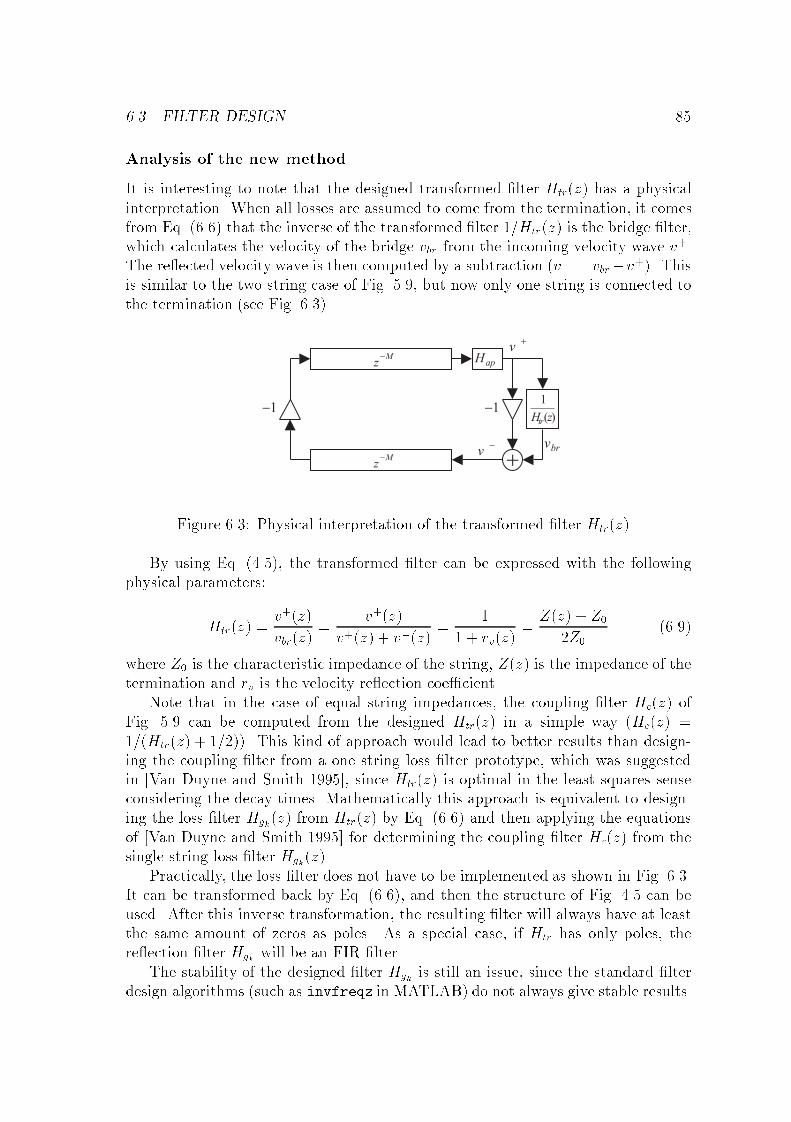
6.3. FILTER DESIGN 85

Analysis of the new method

It is interesting to note that the designed transformed �lter Htr(z) has a physicalinterpretation. When all losses are assumed to come from the termination, it comesfrom Eq. (6.6) that the inverse of the transformed �lter 1=Htr(z) is the bridge �lter,which calculates the velocity of the bridge vbr from the incoming velocity wave v+.The re�ected velocity wave is then computed by a subtraction (v� = vbr�v+). Thisis similar to the two string case of Fig. 5.9, but now only one string is connected tothe termination (see Fig. 6.3).

Figure 6.3: Physical interpretation of the transformed �lter Htr(z).

By using Eq. (4.5), the transformed �lter can be expressed with the followingphysical parameters:

Htr(z) =v+(z)

vbr(z)=

v+(z)

v+(z) + v�(z)=

1

1 + rv(z)=Z(z) + Z0

2Z0(6.9)

where Z0 is the characteristic impedance of the string, Z(z) is the impedance of thetermination and rv is the velocity re�ection coe�cient.

Note that in the case of equal string impedances, the coupling �lter Hc(z) ofFig. 5.9 can be computed from the designed Htr(z) in a simple way (Hc(z) =1=(Htr(z) + 1=2)). This kind of approach would lead to better results than design-ing the coupling �lter from a one string loss �lter prototype, which was suggestedin [Van Duyne and Smith 1995], since Htr(z) is optimal in the least squares senseconsidering the decay times. Mathematically this approach is equivalent to design-ing the loss �lter Hgk(z) from Htr(z) by Eq. (6.6) and then applying the equationsof [Van Duyne and Smith 1995] for determining the coupling �lter Hc(z) from thesingle string loss �lter Hgk(z).

Practically, the loss �lter does not have to be implemented as shown in Fig. 6.3.It can be transformed back by Eq. (6.6), and then the structure of Fig. 4.5 can beused. After this inverse transformation, the resulting �lter will always have at leastthe same amount of zeros as poles. As a special case, if Htr has only poles, there�ection �lter Hgk will be an FIR �lter.

The stability of the designed �lter Hgk is still an issue, since the standard �lterdesign algorithms (such as invfreqz in MATLAB) do not always give stable results.

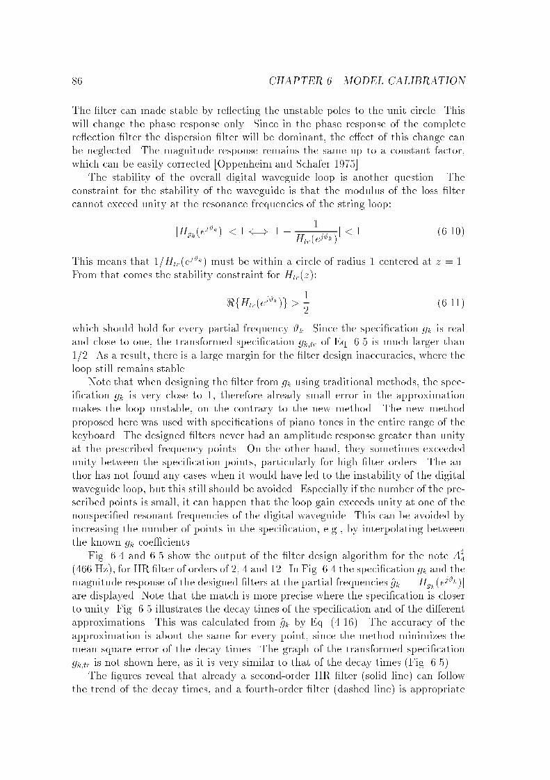
86 CHAPTER 6. MODEL CALIBRATION

The �lter can made stable by re�ecting the unstable poles to the unit circle. Thiswill change the phase response only. Since in the phase response of the completere�ection �lter the dispersion �lter will be dominant, the e�ect of this change canbe neglected. The magnitude response remains the same up to a constant factor,which can be easily corrected [Oppenheim and Schafer 1975].

The stability of the overall digital waveguide loop is another question. Theconstraint for the stability of the waveguide is that the modulus of the loss �ltercannot exceed unity at the resonance frequencies of the string loop:

jHgk(ej#k)j < 1() j1 � 1

Htr(ej#k)j < 1 (6.10)

This means that 1=Htr(ej#k) must be within a circle of radius 1 centered at z = 1.From that comes the stability constraint for Htr(z):

<fHtr(ej#k)g > 1

2(6.11)

which should hold for every partial frequency #k. Since the speci�cation gk is realand close to one, the transformed speci�cation gk;tr of Eq. 6.5 is much larger than1=2. As a result, there is a large margin for the �lter design inaccuracies, where theloop still remains stable.

Note that when designing the �lter from gk using traditional methods, the spec-i�cation gk is very close to 1, therefore already small error in the approximationmakes the loop unstable, on the contrary to the new method. The new methodproposed here was used with speci�cations of piano tones in the entire range of thekeyboard. The designed �lters never had an amplitude response greater than unityat the prescribed frequency points. On the other hand, they sometimes exceededunity between the speci�cation points, particularly for high �lter orders. The au-thor has not found any cases when it would have led to the instability of the digitalwaveguide loop, but this still should be avoided. Especially if the number of the pre-scribed points is small, it can happen that the loop gain exceeds unity at one of thenonspeci�ed resonant frequencies of the digital waveguide. This can be avoided byincreasing the number of points in the speci�cation, e.g., by interpolating betweenthe known gk coe�cients.

Fig. 6.4 and 6.5 show the output of the �lter design algorithm for the note A]4

(466 Hz), for IIR �lter of orders of 2, 4 and 12. In Fig. 6.4 the speci�cation gk and themagnitude response of the designed �lters at the partial frequencies gk = jHgk (e

j#k)jare displayed. Note that the match is more precise where the speci�cation is closerto unity. Fig. 6.5 illustrates the decay times of the speci�cation and of the di�erentapproximations. This was calculated from gk by Eq. (4.16). The accuracy of theapproximation is about the same for every point, since the method minimizes themean square error of the decay times. The graph of the transformed speci�cationgk;tr is not shown here, as it is very similar to that of the decay times (Fig. 6.5).

The �gures reveal that already a second-order IIR �lter (solid line) can followthe trend of the decay times, and a fourth-order �lter (dashed line) is appropriate

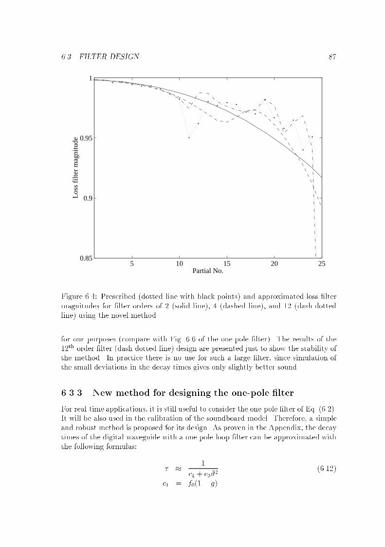
6.3. FILTER DESIGN 87

5 10 15 20 250.85

0.9

0.95

1

Partial No.

Loss

filte

r m

agni

tude

Figure 6.4: Prescribed (dotted line with black points) and approximated loss �ltermagnitudes for �lter orders of 2 (solid line), 4 (dashed line), and 12 (dash-dottedline) using the novel method.

for our purposes (compare with Fig. 6.6 of the one-pole �lter). The results of the12th-order �lter (dash-dotted line) design are presented just to show the stability ofthe method. In practice there is no use for such a large �lter, since simulation ofthe small deviations in the decay times gives only slightly better sound.

6.3.3 New method for designing the one-pole �lter

For real-time applications, it is still useful to consider the one-pole �lter of Eq. (6.2).It will be also used in the calibration of the soundboard model. Therefore, a simpleand robust method is proposed for its design. As proven in the Appendix, the decaytimes of the digital waveguide with a one-pole loop �lter can be approximated withthe following formulas:

� � 1

c1 + c3#2(6.12)

c1 = f0(1 � g)

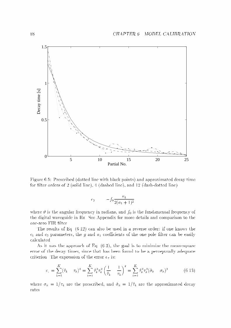
88 CHAPTER 6. MODEL CALIBRATION

5 10 15 20 250

0.5

1

1.5

Partial No.

Dec

ay ti

me

[s]

Figure 6.5: Prescribed (dotted line with black points) and approximated decay timefor �lter orders of 2 (solid line), 4 (dashed line), and 12 (dash-dotted line).

c3 = �f0 a12(a1 + 1)2

where # is the angular frequency in radians, and f0 is the fundamental frequency ofthe digital waveguide in Hz. See Appendix for more details and comparison to theone-zero FIR �lter.

The results of Eq. (6.12) can also be used in a reverse order: if one knows thec1 and c3 parameters, the g and a1 coe�cients of the one-pole �lter can be easilycalculated.

As it was the approach of Eq. (6.3), the goal is to minimize the mean-squareerror of the decay times, since that has been found to be a perceptually adequatecriterion. The expression of the error e� is:

e� =KXk=1

(�k � �k)2 =

KXk=1

� 2k �2k

�1

�k� 1

�k

�2=

KXk=1

� 2k �2k (�k � �k)

2 (6.13)

where �k = 1=�k are the prescribed, and �k = 1=�k are the approximated decayrates.

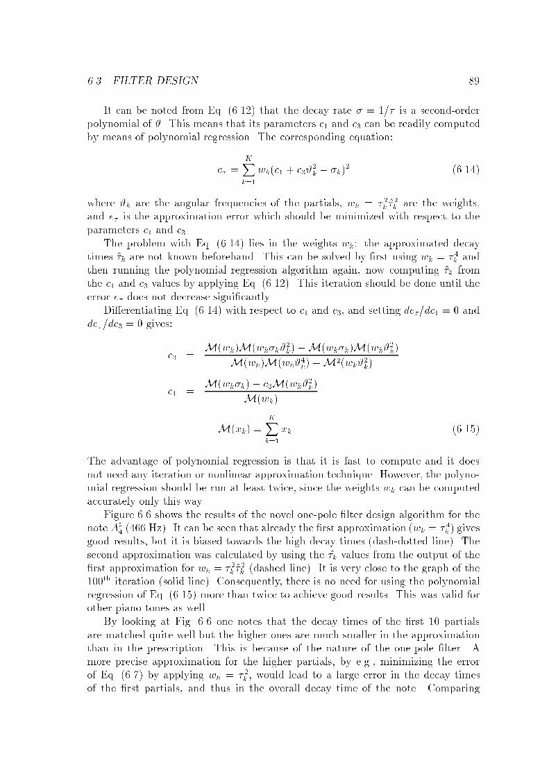
6.3. FILTER DESIGN 89

It can be noted from Eq. (6.12) that the decay rate � = 1=� is a second-orderpolynomial of #. This means that its parameters c1 and c3 can be readily computedby means of polynomial regression. The corresponding equation:

e� =KXk=1

wk(c1 + c3#2k � �k)

2 (6.14)

where #k are the angular frequencies of the partials, wk = � 2k �2k are the weights,

and e� is the approximation error which should be minimized with respect to theparameters c1 and c3.

The problem with Eq. (6.14) lies in the weights wk: the approximated decaytimes �k are not known beforehand. This can be solved by �rst using wk = � 4k andthen running the polynomial regression algorithm again, now computing �k fromthe c1 and c3 values by applying Eq. (6.12). This iteration should be done until theerror e� does not decrease signi�cantly.

Di�erentiating Eq. (6.14) with respect to c1 and c3, and setting de�=dc1 = 0 andde�=dc3 = 0 gives:

c3 =M(wk)M(wk�k#

2k)�M(wk�k)M(wk#

2k)

M(wk)M(wk#4k)�M2(wk#2k)

c1 =M(wk�k)� c3M(wk#

2k)

M(wk)

M(xk) =KXk=1

xk (6.15)

The advantage of polynomial regression is that it is fast to compute and it doesnot need any iteration or nonlinear approximation technique. However, the polyno-mial regression should be run at least twice, since the weights wk can be computedaccurately only this way.

Figure 6.6 shows the results of the novel one-pole �lter design algorithm for thenote A]

4 (466 Hz). It can be seen that already the �rst approximation (wk = � 4k ) givesgood results, but it is biased towards the high decay times (dash-dotted line). Thesecond approximation was calculated by using the �k values from the output of the�rst approximation for wk = � 2k �

2k (dashed line). It is very close to the graph of the

100th iteration (solid line). Consequently, there is no need for using the polynomialregression of Eq. (6.15) more than twice to achieve good results. This was valid forother piano tones as well.

By looking at Fig. 6.6 one notes that the decay times of the �rst 10 partialsare matched quite well but the higher ones are much smaller in the approximationthan in the prescription. This is because of the nature of the one-pole �lter. Amore precise approximation for the higher partials, by e.g., minimizing the errorof Eq. (6.7) by applying wk = � 2k , would lead to a large error in the decay timesof the �rst partials, and thus in the overall decay time of the note. Comparing

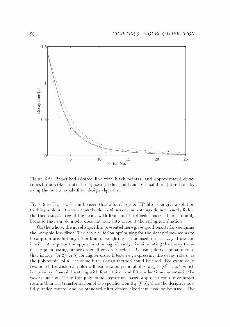
90 CHAPTER 6. MODEL CALIBRATION

5 10 15 20 250

0.5

1

1.5

Partial No.

Dec

ay ti

me

[s]

Figure 6.6: Prescribed (dotted line with black points), and approximated decaytimes for one (dash-dotted line), two (dashed line) and 100 (solid line) iterations byusing the new one-pole �lter design algorithm.

Fig. 6.6 to Fig. 6.5, it can be seen that a fourth-order IIR �lter can give a solutionto this problem. It seems that the decay times of piano strings do not exactly followthe theoretical curve of the string with �rst- and third-order losses. This is mainlybecause that simple model does not take into account the string termination.

On the whole, the novel algorithm presented here gives good results for designingthe one-pole loss �lter. The error criterion optimizing for the decay times seems tobe appropriate, but any other kind of weighting can be used, if necessary. However,it will not improve the approximation signi�cantly: for simulating the decay timesof the piano string higher-order �lters are needed. By using derivation similar tothat in Eqs. (A.2)-(A.5) for higher-order �lters, i.e., expressing the decay rate � asthe polynomial of #, the same �lter design method could be used. For example, atwo-pole �lter with real poles will lead to a polynomial of � � c1+c3#

2+c5#4, which

is the decay time of the string with �rst-, third- and �fth-order time derivates in thewave equation. Using this polynomial regression based approach could give betterresults than the transformation of the speci�cation Eq. (6.5), since the design is nowfully under control and no standard �lter design algorithm need to be used. The

6.3. FILTER DESIGN 91

disadvantage of this technique is that quite much analytical work is needed, makingit unrealizable for high �lter orders. On the contrary, the transformation methodcan be used for those cases easily. The author suggests the polynomial regressionbased approach for low �lter orders, such as one or two, and the transformationmethod for higher ones.

6.3.4 Designing the dispersion �lter

The dispersion of the string is implemented by an allpass �lter. This ensures that thedecay times will be controlled by the loss �lter and the stability of the delay loop willdepend on the loss �lter only. However, these are in�uenced by the dispersion �lter,since it sets the resonance frequencies of the digital waveguide. By reformulatingEq. (4.18) the e�ective length Deff of the digital waveguide should be:

Deff (fk) =fsk

fk= Dwg +DrF (fk) (6.16)

where fs is the sampling frequency, fk is the frequency of the partial k, Dwg = N isthe phase delay introduced by delay lines of the digital waveguide, and DrF is thephase delay of the re�ection �lter.

Since the phase delay of the loss �lter can be neglected when designing thedispersion �lter, the speci�cation for the dispersion �lter will be:

Ddisp(fk) =fsk

fk�Dwg (6.17)

When the inharmonicity indices fk=(kf0) increase with frequency, which is the casefor real strings, this will lead to a monotonically decreasing speci�cation. The delayof the digital waveguide Dwg is a free parameter during the �lter design.

Here the approach suggested by Van Duyne and Smith [1994] is taken. Thedispersion �lter is a series of �rst-order allpass �lters, whose transfer function is asfollows:

H1ap(z) =a1 + z�1

1 + a1z�1(6.18)

The phase delay of such a �lter is similar to that what is needed for simulating theinharmonicity of real strings. Unfortunately, one �lter is not enough to implementthe necessary phase delay. Therefore more �rst-order allpass �lters are connected inseries [Van Duyne and Smith 1994].

In [Van Duyne and Smith 1994] using the same a1 coe�cients for all the �rst-order allpass �lters was motivated by computational reasons. They suggested amultiplier-free implementation with a1 values being a power of 2 or 1 minus a powerof two. Here we do not restrict ourselves to these kind of coe�cients, a1 can be anyrational number. However, using the same a1 for all the �lters in the chain simpli�esthe �lter design process considerably.

The �lter coe�cient a1 was determined by minimizing the least squares errorin the phase delay. A weighting was used which gave more emphasis to the lower

92 CHAPTER 6. MODEL CALIBRATION

partials. The number of �rst-order allpass �lters in the chain was a given parameter.For the lowest notes of the piano, 16 �rst-order allpass �lters were connected in chain.For the higher ones, this number was 8 or 4. This was found to give satisfactory sonicresults, but it is not optimal in any sense. More work has to be done concerningthis part of the model.

Rocchesso and Scalcon [1996] suggested a more re�ned method by using theallpass �lter design technique of Lang and Laakso [1994]. The analysis of thattechnique and the sonic comparison to the simple method applied here will be apart of future research. The results of listening tests by Rocchesso and Scalcon[1999] and Järveläinen et al. [1999] could be also incorporated in the �lter design.

6.3.5 Setting the fundamental frequency

As mentioned earlier, the phase delay of the digital waveguide loop should be veryaccurate at the fundamental frequency of the note. If it is not so, the correspondingnote will be out of tune. Once the loss and the dispersion �lters are designed, thelength of the digital waveguide D(f0) at the fundamental frequency f0 of the toneshould be:

D(f0) = Dwg +Dfd =fsf0�Dgk (f0)�Ddisp(f0) (6.19)

where Dgk and Ddisp are the phase delay of the loss and dispersion �lters, respec-tively.

The prescribed length of the waveguideD(f0) is not an integer. On the contrary,only an integer phase delay can be implemented with delay lines. The solution is touse fractional delay �lters [Välimäki 1995; Laakso et al. 1996] in series with the delayline. Here a �rst-order allpass �lter was used for this purpose, as proposed in [Smith1983; Ja�e and Smith 1983], whose transfer function is described by Eq. (6.18). Theinteger part of D(f0) will be implemented as the delay line of the digital waveguidewith a length of Dwg = bD(f0) � 0:5c, and the fractional part will be realizedwith a �rst-order allpass �lter with a phase delay of Dfd(f0) = D(f0)�Dwg at thefundamental frequency f0. The resulting fractional delay will be 0:5 � Dfd(f0) < 1:5which is the optimal range for the �rst-order allpass �lter [Välimäki 1995]. Thea1 coe�cient of the allpass �lter can be approximately calculated as a1 = (1 �Dfd(f0))=(1 +Dfd(f0)) [Smith 1983; Ja�e and Smith 1983; Välimäki 1995].

6.4 Calibration of the resonator bank

This section will deal with the calibration of the novel resonator bank implemen-tation for beating and two-stage decay. Since the resonator based approach formodeling these e�ects is new, no analysis techniques could be found in the litera-ture. The problem is similar to what is needed for designing the �lters for the modelof Fig. 5.10, but the corresponding paper [Daudet et al. 1999] only says that theauthors used parametric modeling. The method presented here has the advantage

6.4. CALIBRATION OF THE RESONATOR BANK 93

that there is no nonlinear optimization needed and it is robust for real piano tones.Consequently, this new approach could also be useful for calibrating the model ofDaudet et al. [1999].

The structure was described in Section 5.3.3, and now the task is to determinethe poles pk and the amplitude coe�cients ak for the resonators (see Eqs. (5.2) and(5.3)). To be able to do that, �rst we have to investigate what kind of amplitudeenvelopes can arise from two exponentially damping sinusoids.

6.4.1 Analysis of the two-mode model

Our starting-point is the two-mode model, with two exponentially damping sinu-soids, whose initial amplitude, phase, decay time and fundamental frequency pa-rameters can all di�er. This simpli�ed model was found useful in describing themain features of beating and two stage decay [Weinreich 1977]. The physics of thesetwo phenomena was described in Section 2.2.1. Let us assume that the parametersof the two modes are already known. Then the sum of the two modes is:

x(t) = A1e�

t�1 sin(2�f1t+ '1) +A2e

�t�2 sin(2�f2t+ '2) (6.20)

where A1 and A2 are the initial amplitudes, '1 and '2 are the initial phases, f1 andf2 are the frequencies, and �1 and �2 are the decay times of the two modes.

To simplify the derivation, the following notation will be used:

a = A1e�

t�1

b = A2e�

t�2

� = 2�f1t+ '1

� = 2�f2t+ '2 (6.21)

Accordingly, the sum of the two modes can be written as:

x(t) = a sin�+ b sin� =a+ b

2(sin�+ sin�) +

a� b

2(sin� � sin �)

=

(a+ b) cos

�� �

2

!sin

�+ �

2+

(a� b) sin

�� �

2

!cos

� + �

2(6.22)

Since f1 � f2, Eq. (6.22) can be seen as a sum of an amplitude modulated sineand an amplitude modulated cosine function. We are not interested here in theinstantaneous phase or frequency of the resulted signal, but in the evolution of themodulating wave. The amplitude envelope A(t) of the signal x(t) will be:

A(t) =

s(a+ b)2 cos2

� � �

2+ (a� b)2 sin2

�� �

2

=

vuuta2 + b2 + 2ab

cos2

�� �

2� sin2

� � �

2

!

=qa2 + b2 + 2ab cos(�� �) (6.23)

94 CHAPTER 6. MODEL CALIBRATION

The geometrical interpretation of this equation is the length of the sum of twovectors in the x-y plane, whose lengths are a and b, and their angles to the x-axisare � and �.

By substituting the original variables according to Eq. (6.21) we obtain:

A(t) =

sA2

1e�

2t�1 +A2

2e�

2t�2 + 2A1A2e

�t

�1

�1+ 1

�2

�cos(2�(f1 � f2)t+ '1 � '2) (6.24)

This is the amplitude envelope of the signal x(t). It covers not only the beating, butalso the decay of the sound. We can have better insight to beating if we reformulateEq. (6.20):

x(t) = A1e�

t�1

sin(2�f1t+ '1) +

A2

A1e�t

�1

�2�

1

�1

�sin(2�f2t+ '2)

!

= A1e�

t�1 xrel(t) (6.25)

Now we have factored out the general exponential decay and normalized the initialamplitudes. The amplitude envelope b(t) of the normalized signal xrel(t) will be:

b(t) =

r1 +A2

be�

2t�b + 2Abe

�t�b cos(2�fbt+ 'b)

Ab =A2

A1

�b =1

�2� 1

�1fb = f1 � f2

'b = '1 � '2 (6.26)

We see from Eq. (6.26) that for Ab � 0 the upper and lower limits for the beatingsignal b(t) are:

j1�Abe�

t�b j � b(t) � 1 +Abe

�t�b (6.27)

From Eq. (6.27) follows that the beating is the largest when Abe�t=�b = 1, which is

when the amplitude envelope of the two decaying sinusoids cross. Before this point,the decay grows, and after that decays. Note that the largest beating does not referto the maximal b(t) value, but to the maximal relative di�erence between the lowerand upper bounds of b(t), which is when the lower bound equals to zero.

For those cases where 0 � Abe�t=�b � 1, the beating b(t) can be approximated

with an exponentially rising or decaying sinusoid:

b(t) � 1 +Abe�

t�b cos(2�fbt+ 'b) (6.28)

The smaller the Abe�t=�b value, the more accurate the approximation. It comes form

the constraint Abe�t=�b � 1 that Eq. (6.28) handles only either the decaying, or the

growing part of the beating. If we separate these parts during the analysis of realamplitude envelopes, and �t this kind of curve on one of them, we can get all theparameters which characterize the two-mode model. However, the synthesis modelwill behave as in Eq. (6.26).

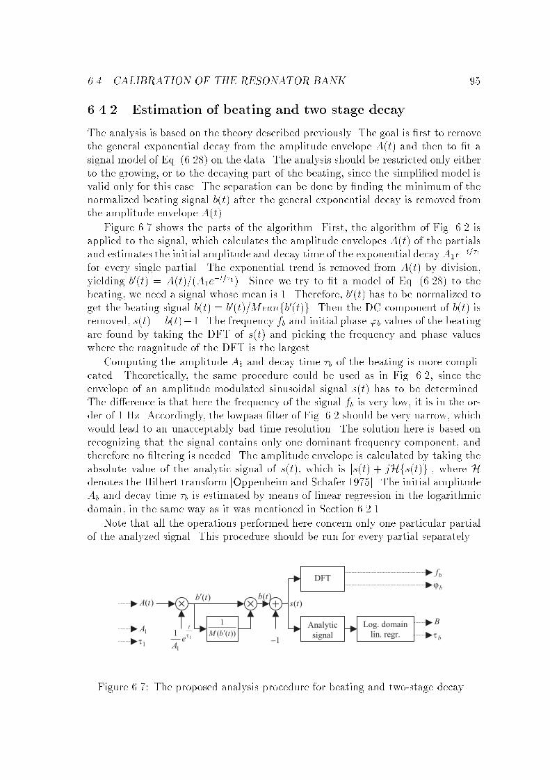
6.4. CALIBRATION OF THE RESONATOR BANK 95

6.4.2 Estimation of beating and two stage decay

The analysis is based on the theory described previously. The goal is �rst to removethe general exponential decay from the amplitude envelope A(t) and then to �t asignal model of Eq. (6.28) on the data. The analysis should be restricted only eitherto the growing, or to the decaying part of the beating, since the simpli�ed model isvalid only for this case. The separation can be done by �nding the minimum of thenormalized beating signal b(t) after the general exponential decay is removed fromthe amplitude envelope A(t).

Figure 6.7 shows the parts of the algorithm. First, the algorithm of Fig. 6.2 isapplied to the signal, which calculates the amplitude envelopes A(t) of the partialsand estimates the initial amplitude and decay time of the exponential decay A1e

�t=�1

for every single partial. The exponential trend is removed from A(t) by division,yielding b0(t) = A(t)=(A1e

�t=�1). Since we try to �t a model of Eq. (6.28) to thebeating, we need a signal whose mean is 1. Therefore, b0(t) has to be normalized toget the beating signal b(t) = b0(t)=Meanfb0(t)g. Then the DC component of b(t) isremoved, s(t) = b(t)�1. The frequency fb and initial phase 'b values of the beatingare found by taking the DFT of s(t) and picking the frequency and phase valueswhere the magnitude of the DFT is the largest.

Computing the amplitude Ab and decay time �b of the beating is more compli-cated. Theoretically, the same procedure could be used as in Fig. 6.2, since theenvelope of an amplitude modulated sinusoidal signal s(t) has to be determined.The di�erence is that here the frequency of the signal fb is very low, it is in the or-der of 1 Hz. Accordingly, the lowpass �lter of Fig. 6.2 should be very narrow, whichwould lead to an unacceptably bad time resolution. The solution here is based onrecognizing that the signal contains only one dominant frequency component, andtherefore no �ltering is needed. The amplitude envelope is calculated by taking theabsolute value of the analytic signal of s(t), which is js(t) + jHfs(t)gj, where Hdenotes the Hilbert transform [Oppenheim and Schafer 1975]. The initial amplitudeAb and decay time �b is estimated by means of linear regression in the logarithmicdomain, in the same way as it was mentioned in Section 6.2.1.

Note that all the operations performed here concern only one particular partialof the analyzed signal. This procedure should be run for every partial separately.

Figure 6.7: The proposed analysis procedure for beating and two-stage decay.

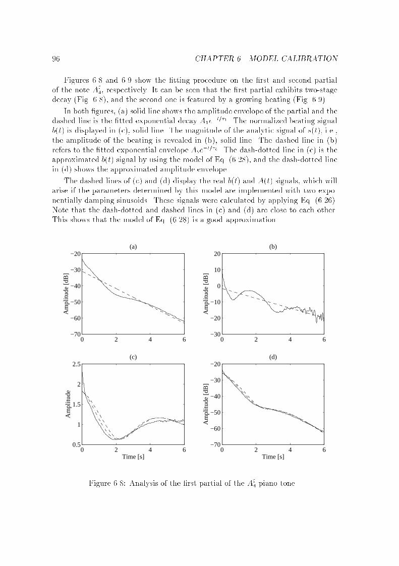
96 CHAPTER 6. MODEL CALIBRATION

Figures 6.8 and 6.9 show the �tting procedure on the �rst and second partialof the note A]

4, respectively. It can be seen that the �rst partial exhibits two-stagedecay (Fig. 6.8), and the second one is featured by a growing beating (Fig. 6.9).

In both �gures, (a) solid line shows the amplitude envelope of the partial and thedashed line is the �tted exponential decay A1e

�t=�1. The normalized beating signalb(t) is displayed in (c), solid line. The magnitude of the analytic signal of s(t), i.e.,the amplitude of the beating is revealed in (b), solid line. The dashed line in (b)refers to the �tted exponential envelope Abe

�t=�b. The dash-dotted line in (c) is theapproximated b(t) signal by using the model of Eq. (6.28), and the dash-dotted linein (d) shows the approximated amplitude envelope.

The dashed lines of (c) and (d) display the real b(t) and A(t) signals, which willarise if the parameters determined by this model are implemented with two expo-nentially damping sinusoids. These signals were calculated by applying Eq. (6.26).Note that the dash-dotted and dashed lines in (c) and (d) are close to each other.This shows that the model of Eq. (6.28) is a good approximation.

0 2 4 6−70

−60

−50

−40

−30

−20(a)

Am

plitu

de [d

B]

0 2 4 6−30

−20

−10

0

10

20(b)

Am

plitu

de [d

B]

0 2 4 60.5

1

1.5

2

2.5(c)

Time [s]

Am

plitu

de

0 2 4 6−70

−60

−50

−40

−30

−20(d)

Time [s]

Am

plitu

de [d

B]

Figure 6.8: Analysis of the �rst partial of the A]4 piano tone.

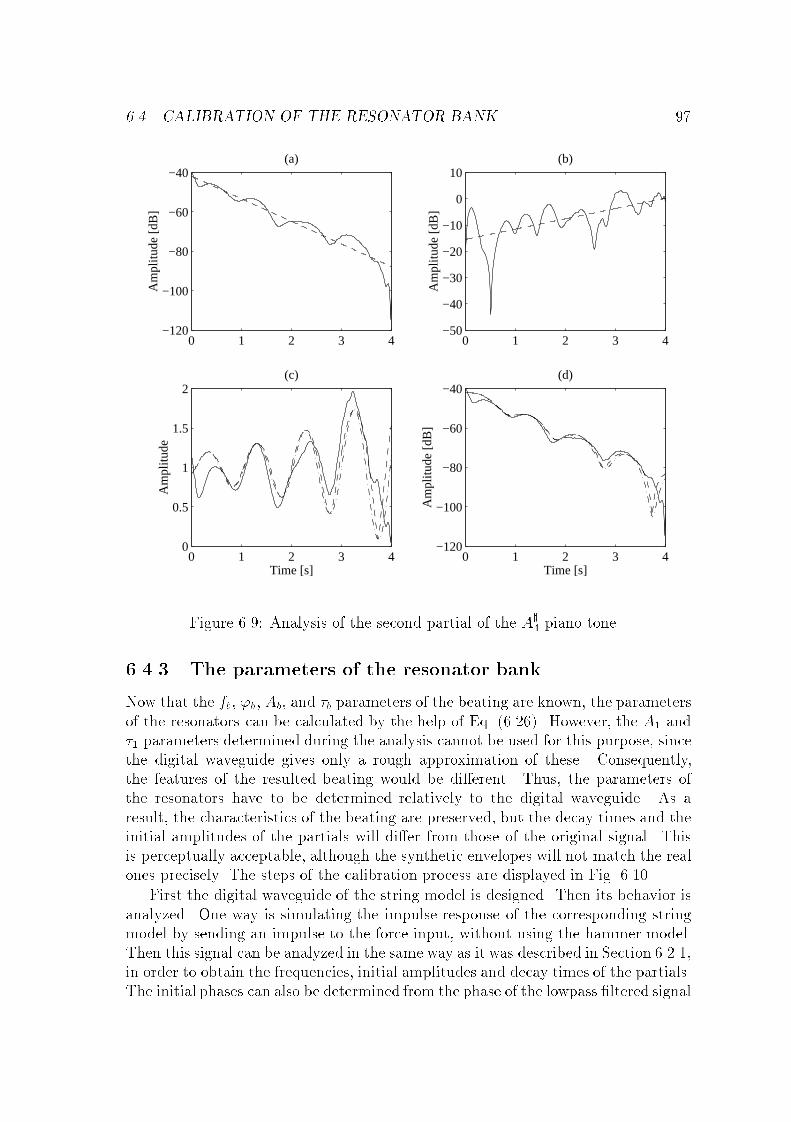
6.4. CALIBRATION OF THE RESONATOR BANK 97

0 1 2 3 4−120

−100

−80

−60

−40(a)

Am

plitu

de [d

B]

0 1 2 3 4−50

−40

−30

−20

−10

0

10(b)

Am

plitu

de [d

B]

0 1 2 3 40

0.5

1

1.5

2(c)

Time [s]

Am

plitu

de

0 1 2 3 4−120

−100

−80

−60

−40(d)

Time [s]

Am

plitu

de [d

B]

Figure 6.9: Analysis of the second partial of the A]4 piano tone.

6.4.3 The parameters of the resonator bank

Now that the fb, 'b, Ab, and �b parameters of the beating are known, the parametersof the resonators can be calculated by the help of Eq. (6.26). However, the A1 and�1 parameters determined during the analysis cannot be used for this purpose, sincethe digital waveguide gives only a rough approximation of these. Consequently,the features of the resulted beating would be di�erent. Thus, the parameters ofthe resonators have to be determined relatively to the digital waveguide. As aresult, the characteristics of the beating are preserved, but the decay times and theinitial amplitudes of the partials will di�er from those of the original signal. Thisis perceptually acceptable, although the synthetic envelopes will not match the realones precisely. The steps of the calibration process are displayed in Fig. 6.10.

First the digital waveguide of the string model is designed. Then its behavior isanalyzed. One way is simulating the impulse response of the corresponding stringmodel by sending an impulse to the force input, without using the hammer model.Then this signal can be analyzed in the same way as it was described in Section 6.2.1,in order to obtain the frequencies, initial amplitudes and decay times of the partials.The initial phases can also be determined from the phase of the lowpass �ltered signal

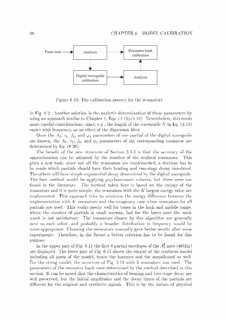
98 CHAPTER 6. MODEL CALIBRATION

Figure 6.10: The calibration process for the resonators.

in Fig. 6.2. Another solution is the analytic determination of these parameters byusing an approach similar to Chapter 4, Eqs. (4.15)-(4.18). Nevertheless, this needsmore careful considerations, since, e.g., the length of the waveguide N in Eq. (4.15)varies with frequency, as an e�ect of the dispersion �lter.

Once the A1, �1, f1, and '1 parameters of one partial of the digital waveguideare known, the A2, �2, f2, and '2 parameters of the corresponding resonator aredetermined by Eq. (6.26).

The bene�t of the new structure of Section 5.3.3 is that the accuracy of theapproximation can be adjusted by the number of the realized resonators. Thisgives a new task: since not all the resonators are implemented, a decision has tobe made which partials should have their beating and two-stage decay simulated.The others will have simple exponential decay determined by the digital waveguide.The best method would be applying psychoacoustic criteria, but these were notfound in the literature. The method taken here is based on the energy of theresonators and it is quite simple: the resonators with the K largest energy value areimplemented. This approach tries to minimize the energy di�erence between theimplementation with K resonators and the imaginary case when resonators for allpartials are used. This works pretty well for tones in the high and middle range,where the number of partials is small anyway, but for the lower ones the sonicresult is not satisfactory. The resonators chosen by this algorithm are generallynext to each other, and probably a broader distribution in frequency would bemore appropriate. Choosing the resonators manually gave better results after someexperiments. Therefore, in the future a better criterion has to be found for thispurpose.

In the upper part of Fig. 6.11 the �rst 8 partial envelopes of the A]4 note (466Hz)

are displayed. The lower part of Fig. 6.11 shows the output of the synthesis modelincluding all parts of the model, hence the hammer and the soundboard as well.For the string model, the structure of Fig. 5.12 with 5 resonators was used. Theparameters of the resonator bank were determined by the method described in thissection. It can be noted that the characteristics of beating and two-stage decay arewell preserved, but the initial amplitudes and the decay times of the partials aredi�erent for the original and synthetic signals. This is by the nature of physical

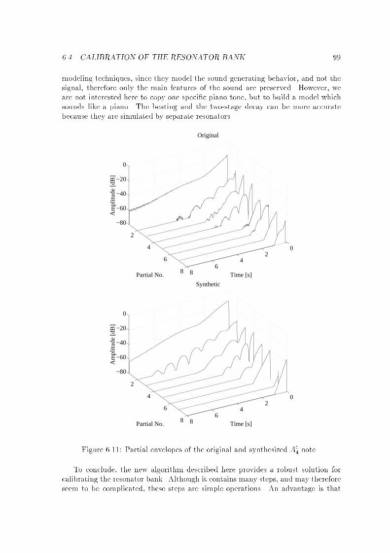
6.4. CALIBRATION OF THE RESONATOR BANK 99

modeling techniques, since they model the sound generating behavior, and not thesignal, therefore only the main features of the sound are preserved. However, weare not interested here to copy one speci�c piano tone, but to build a model whichsounds like a piano. The beating and the two-stage decay can be more accuratebecause they are simulated by separate resonators.

02

46

8

2

4

6

8

−80

−60

−40

−20

0

Time [s]

Original

Partial No.

Am

plitu

de [d

B]

02

46

8

2

4

6

8

−80

−60

−40

−20

0

Time [s]

Synthetic

Partial No.

Am

plitu

de [d

B]

Figure 6.11: Partial envelopes of the original and synthesized A]4 note.

To conclude, the new algorithm described here provides a robust solution forcalibrating the resonator bank. Although it contains many steps, and may thereforeseem to be complicated, these steps are simple operations. An advantage is that

100 CHAPTER 6. MODEL CALIBRATION

there is no need for any iteration or nonlinear optimization, and this ensures thestability of the algorithm. The method was found to be reliable for all analyzedpiano tones.

The problem of the technique described here is that it should be done for allpiano notes. The decay times for re�ection �lter design can be interpolated fromone or two measurements in every octave. On the contrary, the characteristics ofbeating and two-stage decay are so di�erent from note to note that these cannotbe determined by interpolation between the measured notes. By measuring theimpedance at some points along the bridge and calculating the parameters fromthat could possibly overcome this problem. Then the impedance curve should besampled at the modal frequencies of the string and the parameters of the beatingcould be calculated using the equations described in [Weinreich 1977]. This probablywould not give the same features as of the original tones, but it would give physicallymeaningful behavior. The robustness of such a method is a question, since the noisein impedance measurement can make the whole process unstable. Therefore, theauthor suggests measuring all piano tones and using the method based on partialenvelopes. The analysis process is automatic. The only time-consuming operationis the recording of the 88 piano notes.

6.5 Calibration of the soundboard model

The calibration of the soundboard model consists of two parts: determining theparameters of the feedback delay network and designing the shaping �lter.

6.5.1 Parameters of the feedback delay network

The feedback delay network is described by the variables of Eq. (5.4) and by theloss �lters Hk(z) connected to the delay lines in series. Choosing the length of thedelay lines was already discussed in Section 5.4.3.

The feedback matrix A was �rst chosen to be a special case of a circular matrix,where all the eigenvalues of A are at 1 expect one, which is at �1. This results ina feedback matrix, where the elements are the same expect the ones in the diagonal[Rocchesso and Smith 1997]. This leads to a very e�cient implementation. However,when the number of delay lines is higher than four, the magnitude of the elementsin the diagonal will be larger than the others. Consequently, the delay lines will getmore input from their own output than desired, and this results in more harmonictimbre. Better solutions can be obtained by shifting the feedback matrix to theright with one step. This spreads the eigenvalues of the feedback matrix around theunit circle [Rocchesso and Smith 1997]. Thus, the �rst row of the circular feedbackmatrix in our case is: [�1=4; 1 � 1=4;�1=4;�1=4;�1=4;�1=4;�1=4;�1=4].

The input and output coe�cient vectors b and c were chosen as suggested in[Rocchesso and Smith 1997] to avoid coloration in arti�cial reverberators. However,the equations in [Rocchesso and Smith 1997] are valid when the lengths of the delay

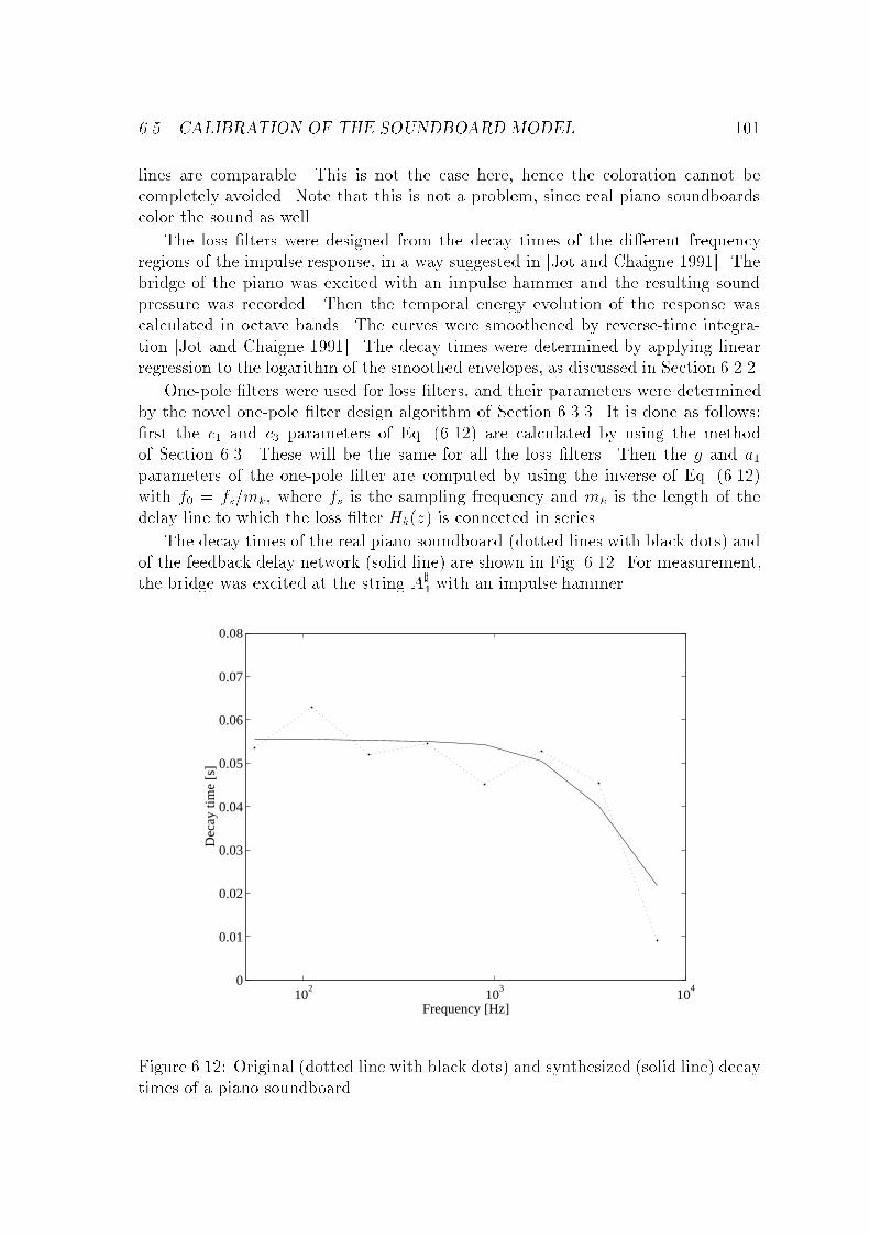
6.5. CALIBRATION OF THE SOUNDBOARD MODEL 101

lines are comparable. This is not the case here, hence the coloration cannot becompletely avoided. Note that this is not a problem, since real piano soundboardscolor the sound as well.

The loss �lters were designed from the decay times of the di�erent frequencyregions of the impulse response, in a way suggested in [Jot and Chaigne 1991]. Thebridge of the piano was excited with an impulse hammer and the resulting soundpressure was recorded. Then the temporal energy evolution of the response wascalculated in octave bands. The curves were smoothened by reverse-time integra-tion [Jot and Chaigne 1991]. The decay times were determined by applying linearregression to the logarithm of the smoothed envelopes, as discussed in Section 6.2.2.

One-pole �lters were used for loss �lters, and their parameters were determinedby the novel one-pole �lter design algorithm of Section 6.3.3. It is done as follows:�rst the c1 and c3 parameters of Eq. (6.12) are calculated by using the methodof Section 6.3. These will be the same for all the loss �lters. Then the g and a1parameters of the one-pole �lter are computed by using the inverse of Eq. (6.12)with f0 = fs=mk, where fs is the sampling frequency and mk is the length of thedelay line to which the loss �lter Hk(z) is connected in series.

The decay times of the real piano soundboard (dotted lines with black dots) andof the feedback delay network (solid line) are shown in Fig. 6.12. For measurement,the bridge was excited at the string A]

4 with an impulse hammer.

102

103

104

0

0.01

0.02

0.03

0.04

0.05

0.06

0.07

0.08

Frequency [Hz]

Dec

ay ti

me

[s]

Figure 6.12: Original (dotted line with black dots) and synthesized (solid line) decaytimes of a piano soundboard.

102 CHAPTER 6. MODEL CALIBRATION

It can be seen from Fig. 6.12 that the one-pole �lter can follow only the maintrend of the decay times. However, the perceptual quality of the soundboard modelwith such a simple �lter is already quite high. It seems that there is no needfor very complicated loss �lters to reproduce the general characteristics of a pianosoundboard.

6.5.2 Shaping �lter design

For shaping �lter design, the bridge of the soundboard was excited by an impulsehammer and the force and sound pressure signals were synchronously recorded.Then their spectra were computed by the Discrete Fourier Transform. The transferfunction was obtained by the frequency domain division of the two signals. Unfor-tunately, the noise level of both signals were high. This is especially critical in theforce signal, since its spectrum is in the denominator. Where the force spectrumapproaches zero, the transfer function of the soundboard has high peaks and thisleads to useless results.

This can be avoided by noting that the information content of the force signal isconcentrated only to the �rst hundred samples, since the excitation is of an impulsetype. After the impulse, when the force hammer has lost contact to the bridge, allthe values of the force signal were set to zero. This resulted in a large improvementin the noise level. The reduction is proportional to the length of the force impulseand of the analyzed record, which comes from the length of the pressure signal. Fortypical measurements, the noise energy in the force signal was reduced to the 1/50by this technique.

The impulse response of the soundboard was obtained by the Inverse DiscreteFourier Transform of the transfer function. The shaping �lter Hsh(z) in Fig. 5.14 isthe windowed version of the impulse response. The length of the FIR �lter used inthe model was 100 taps. Using IIR �lters could lead to a more e�cient implementa-tion. However, if the �lter order is high, the �lter design algorithms easily run intostability problems.

The speci�cations for the correction �lters Hhigh(z) and Hlow(z) in Fig. 5.14for the high and low range of the keyboard, respectively, are obtained by dividingthe transfer functions of the soundboard at the high and low range by the transferfunction of the shaping �lter Hsh(z). Then this frequency-domain data is smoothedand the �lters are designed by standard �lter design methods. Typically, second orthird-order IIR �lters give good results.

6.6 Conclusion

In this chapter the calibration of the piano model was outlined. For the loss �lterof the digital waveguide, a new design algorithm was presented. It is based on thetransformation of the speci�cation and optimizes the resulting decay times. Themethod has been found stable even for high �lter orders. A fast and robust algo-

6.6. CONCLUSION 103

rithm was presented for the design of the one-pole loss �lter, founded on polynomialregression. A new algorithm was developed for the measurement of beating and two-stage decay, which can be used for the calibration of the resonator bank. Methodsfor determining the parameters of the soundboard model were also described.

104 CHAPTER 6. MODEL CALIBRATION

Chapter 7

Summary and future directions

7.1 The results

The thesis presented a model for the synthesis of piano sound. The approach isgrounded on physical principles, because the structure of the model follows thatof the real piano. However, the implementations of the di�erent parts are notnecessarily physical. The aim of the author was to �nd the most e�cient fusionof the di�erent sound synthesis approaches.

The acoustical properties of the piano were discussed by both reviewing theresults of the literature and presenting the outcomes of measurements. Implicationswere given for which features of the piano are responsible for the distinctive characterof the timbre. This part of the work forms the basis for the sound synthesis of thepiano.

This was followed in Chapter 4 by the discussion of an e�cient string modelingtechnique: the digital waveguide modeling. The equations describing the digitalwaveguide were given. The fractional expansion of the transfer function resulted ina new approach in considering the behavior of digital waveguide. These equationsallowed the formulation of the equivalent resonator bank structure. When the polesof the digital waveguide are equally distributed along the unit circle, the impulseresponse of the waveguide and the amplitude coe�cients of the resonators are relatedby the Discrete Fourier Transform. For lossy and dispersive digital waveguides,the resonator coe�cients can be determined by solving a set of linear equations.Because of being capable of implementing delay, the resonator bank can be alsoused for simulating nonlinear interaction. This can be bene�cial for modeling largelyinharmonic instruments, such as, mallet percussion or bells.

After presenting the general principles of string modeling, Chapter 5 concen-trated on modeling a speci�c instrument, the piano. The piano model is a combina-tion of di�erent approaches. The physical modeling approach is most advantageousfor those parts of the model which are controlled by the musician. In the case ofthe piano, the input from the outside world is the movement of the hammer and thedampers. Consequently, the hammer is modeled by discretizing the physical equa-tions of real hammers. Since the force signal experienced by the string is in�uenced

105

106 CHAPTER 7. SUMMARY AND FUTURE DIRECTIONS

by the movement of the string at the excitation point, it is essential to implementthe string as a physical model. The basic string behavior is modeled by a digitalwaveguide. A feature of these two parts of the piano model is that all the variablespresent are physical units. The beating and two-stage decay of the piano soundare simulated by a parallel resonator bank. The frequencies and the decay times ofthe resonators are determined through the analysis, however, the initial amplitudesare controlled by the excitation signal, which is computed by the hammer modeland the digital waveguide. This way, even if it is treated in the analysis phase asa signal model, it responds to the variation of impact velocity in a meaningful way.The soundboard of the piano is modeled by a feedback delay network. This can beconsidered as a statistical model of the impulse response of the soundboard since itmatches only its main features. The physical parameters of the soundboard, suchas size, shape, etc., are not visible in the model. Since these parameters cannot bein�uenced by the musician, the nonphysical approach is adequate here. The messageof the thesis is that the secret of e�cient sound synthesis lies in the combination ofdi�erent approaches.

During the description of the piano structure, some new inventions were alsopresented. The thesis pointed out the discontinuity problem, which arises whenan interaction force is taken into the string. Then, solutions to the problem wereproposed. A multi-rate hammer was presented in order to overcome the stabilityproblem of the hammer model. The use of the same structure for modeling thee�ect of dampers was outlined. A resonator bank based technique was introducedfor modeling the beating and two-stage decay. For the realistic simulation of thecharacteristic attack noise of piano sounds a simple technique was proposed. Toresolve the di�erence between the computational load presented by the string modelsof the high and low register, a multi-rate piano model was proposed.

Novel techniques for calibrating the model were also developed. For designing theloss �lter of the digital waveguide, a transformation based technique was presented.The method optimizes the resulting decay times, which has a perceptual sense.The stability of the designed �lter is also assured. Its another advantage is simpleimplementation. In the Appendix, the link between the decay times of a lossy stringand a digital waveguide with a one-pole �lter is described. The equivalence of theone-zero �lter to the one-pole �lter is also outlined. Based on these results, a simpleand reliable algorithm is presented for designing the one-pole �lter. A technique forthe robust estimation of beating and two-stage decay parameters was also presented.

Most of the novelties of the thesis can be applied not only for modeling the piano,but for the synthesis of other musical instruments as well. Some ideas (e.g., about�lter design) may even �nd applications in other �elds of digital signal processing.

7.2. THE FUTURE 107

7.2 The future

The piano model described in the thesis gives good results.1 Nevertheless, there isstill much to do in making the model more e�cient and the sonic outcome morerealistic.

Physical damper models have to be implemented. For their calibration, newmeasurements are needed. This would be useful also from the analytical pointof view, since the e�ect of dampers in real pianos has not been discussed in theliterature.

For the dispersion �lter of the digital waveguide, a better approximation shouldbe found, because this is computationally the heaviest part of the simulation of lowpiano strings. It would be even better to develop a reliable �lter design algorithm,which could design the re�ection �lter as a whole. This could lead to more e�cientimplementation than separating the di�erent parts of the re�ection �lter. Exper-iments have to be made, whether the nonlinear e�ects of piano strings should besimulated.

The data of soundboard measurements used in this study were noisy, and there-fore the calibration of the soundboard model could not be accurately done. Newmeasurements have been already made, but they still have to be processed. It wouldbe also worth to experiment with loss �lters exhibiting di�erent decay times for thedi�erent delay lines in the feedback delay network. Using other type of shaping�lters than simple FIR �lters would lead to more e�cient simulation of the pianosoundboard. The soundboard model could be made more realistic by modelingthe coupled vibrations of the undamped highest strings. An e�cient method forsimulating the e�ect of sustain pedal also has to be developed.

A part of the plans is to implement the piano model in a real-time environment.It would be bene�cial in many ways: it could allow the e�ciency evaluation ofdi�erent parts of the model, and experimenting with the model parameters wouldbe more convenient that way. However, the real motivation is much more personal.The author wishes to play his own instrument...

1Sound examples and the electronic version of this thesis are available at:http://www.acoustics.hut.fi/�bbank

108 CHAPTER 7. SUMMARY AND FUTURE DIRECTIONS

Bibliography

Adrien, J.-M. 1991. The Missing Link: Modal Synthesis, in: G. D. Poli, A. Pic-cialli and C. Roads (eds), Representations of Musical Signals, The MIT Press,Cambridge, Massachusetts, USA, pp. 269�297.

Allen, J. B. and Rabiner, L. R. 1977. A Uni�ed Approach to Short-Time FourierAnalysis and Synthesis, Proceedings of IEEE, pp. 1558�1564.

Ar�b, D. 1979. Digital Synthesis of Complex Spectra by means of Multiplicationof Nonlinear Distorted Sine Waves, Journal of the Audio Engineering Society

27(10): 757�768.

Askenfelt, A. and Jansson, E. V. 1990. From Touch to Vibrations. I: Timing in theGrand Piano Action, Journal of the Acoustical Society of America 88(1): 52�63.

Askenfelt, A. and Jansson, E. V. 1991. From Touch to Vibrations. II: The Mo-tion of the Key and the Hammer, Journal of the Acoustical Society of America

90(5): 2383�2393.

Askenfelt, A. and Jansson, E. V. 1993. From Touch to Vibrations. III: String Motionand Spectra, Journal of the Acoustical Society of America 93(4): 2181�2196.

Bank, B. 2000. Nonlinear Interaction in the Digital Waveguide with the Applica-tion to Piano Sound Synthesis, Proceedings of the International Computer Music

Conference, Berlin, Germany.

Bank, B., Välimäki, V., Sujbert, L. and Karjalainen, M. 2000. E�cient Physics-Based Sound Synthesis of the Piano Using DSP Methods, Proceedings of the 10th

European Signal Processing Conference, Tampere, Finland.

Borin, G. and De Poli, G. 1996. A Hysteretic Hammer-String Interaction Model forPhysical Model Synthesis, Proceedings of the Nordic Acouctical Meeting, Helsinki,Finland, pp. 399�406.

Borin, G., De Poli, G. and Sarti, A. 1992. Sound Synthesis by Dynamic SystemInteraction, in: D. Baggi (ed.), Readings in Computer Generated Music, IEEEComputer Society Press, Los Alamitos, USA, pp. 139�160.

109

110 BIBLIOGRAPHY

Borin, G., Rocchesso, D. and Scalcon, F. 1997. A Physical Piano Model for Mu-sic Performance, Proceedings of the International Computer Music Conference,Thessaloniki, Greece, pp. 350�353.

Boutillon, X. 1988. Model for Piano Hammers: Experimental Determination andDigital Simulation, Journal of the Acoustical Society of America 83(2): 746�754.

Chaigne, A. and Askenfelt, A. 1994a. Numerical Simulations of Piano Strings. I. APhysical Model for a Struck String Using Finite Di�erence Methods, Journal ofthe Acoustical Society of America 95(2): 1112�1118.

Chaigne, A. and Askenfelt, A. 1994b. Numerical Simulations of Piano Strings. II.Comparisons with Measurements and Systematic Exploration of some Hammer-String Parameters, Journal of the Acoustical Society of America 95(3): 1631�1640.

Chowning, J. M. 1973. The Synthesis of Complex Audio Spectra by Means ofFrequency Modulation, Journal of the Audio Engineering Society 21(7): 526�534.Reprinted in C. Roads and J. Strawn, eds. 1985. Foundations of Computer Music.Cambridge, Massachusetts: The MIT Press. pp. 6-29.

Conklin, H. A. 1996a. Design and Tone in the Mechanoacoustic Piano. Part I.Piano Hammers and Tonal E�ects, Journal of the Acoustical Society of America

99(6): 3286�3296.

Conklin, H. A. 1996b. Design and Tone in the Mechanoacoustic Piano. Part II.Piano Structure, Journal of the Acoustical Society of America 100(2): 695�708.

Conklin, H. A. 1996c. Design and Tone in the Mechanoacoustic Piano. Part III.Piano Strings and Scale Design, Journal of the Acoustical Society of America

100(3): 1286�1298.

Conklin, H. A. 1999. Generation of Partials due to Nonlinear Mixing in a StringedInstrument, Journal of the Acoustical Society of America 105(1): 536�545.

Daudet, L., Guillemain, P. and Kronland-Martinet, R. 1999. Resynthesis of PianoStrings Vibrations Based on Physical Modeling, Proceedings of the International

Computer Music Conference, Beijing, China, pp. 48�51.

Ding, Y. and Qian, X. 1997. Processing of Musical Tones Using a CombinedQuadratic Polynomial-Phase Sinusoid and Residual (QUASAR) Signal Model,Journal of the Audio Engineering Society 45(7/8): 571�584.

Erkut, C., Välimäki, V., Karjalainen, M. and Laurson, M. 2000. Excitation of Phys-ical and Expressive Parameters for Model-Based Sound Synthesis of the Classi-cal Guitar, Proceedings of the 108th AES convention, Preprint No. 5114, Paris,France.

BIBLIOGRAPHY 111

Feldtkeller, R. and Zwicker, E. 1956. Das Ohr als Nachrichtenempfänger, S. HirzelVerlag, Stuttgart, Germany, p. 91.

Fletcher, H., Blackham, E. D. and Stratton, R. 1962. Quality of Piano Tones,Journal of the Acoustical Society of America 34(6): 749�761.

Fletcher, N. H. and Rossing, T. D. 1998. The Physics of Musical Instruments,Springer-Verlag, New York, USA, p. 756.

Garnett, G. E. 1987. Modeling Piano Sound Using Digital Waveguide FilteringTechniques, Proceedings of the International Computer Music Conference, Ur-bana, Illinois, USA, pp. 89�95.

Giordano, N. 1997. Simple Model of a Piano Soundboard, Journal of the AcousticalSociety of America 102(2): 1159�1168.

Giordano, N. 1998. Mechanical Impedance of Piano Soundboard, Journal of theAcoustical Society of America 103(4): 2128�2133.

Giordano, N. and Korty, A. J. 1994. Longitudinal Vibrations and the Role of theBridge, Journal of the Acoustical Society of America 96(3): 1549�1556.

Hall, D. E. 1986. Piano String Excitation in the case of Small HammerMass, Journalof the Acoustical Society of America 79(1): 141�147.

Hall, D. E. 1987a. Piano String Excitation II: General Solution for a Hard NarrowHammer, Journal of the Acoustical Society of America 81(2): 535�546.

Hall, D. E. 1987b. Piano String Excitation III: General Solution for a Soft NarrowHammer, Journal of the Acoustical Society of America 81(2): 547�555.

Hall, D. E. and Clark, P. 1987. Piano String Excitation IV: The Question of MissingModes, Journal of the Acoustical Society of America 82(6): 1913�1918.

Hanson, R. J., Anderson, J. M. and Macomber, H. K. 1994. Measurements ofNonlinear E�ects in a Driven Vibrating Wire, Journal of the Acoustical Society

of America 96(3): 1549�1556.

Hikichi, T. and Osaka, N. 1999. An Approach to Sound Morphing based on PhysicalModeling, Proceedings of the International Computer Music Conference, Beijing,China, pp. 108�111.

Hiller, L. and Ruiz, P. 1971a. Synthesizing Musical Sounds by Solving the WaveEquation for Vibrating Objects: Part 1, Journal of the Audio Engineering Society

19(6): 462�470.

Hiller, L. and Ruiz, P. 1971b. Synthesizing Musical Sounds by Solving the WaveEquation for Vibrating Objects: Part 2, Journal of the Audio Engineering Society

19(7): 542�550.

112 BIBLIOGRAPHY

Ja�e, D. A. and Smith, J. O. 1983. Extensions of the Karplus-Strong Plucked-String Algorithm, Computer Music Journal 7(2): 56�69. Also published in RoadsC. (ed). 1989. The Music Machine, pp. 481�494. The MIT Press. Cambridge,Massachusetts, USA.

Jot, J.-M. 1992. An Analysis/Synthesis Approach to Real-Time Arti�cial Rever-beration, Proceedings of the IEEE International Conference on Acoustics, Speech,

and Signal Processing, Vol. 2, San Francisco, California, USA, pp. 221�224.

Jot, J.-M. and Chaigne, A. 1991. Digital Delay Networks for Designing Arti�cialReverberators, Proceedings of the 90th AES convention, Preprint No. 3030, Paris,France.

Järveläinen, H., Välimäki, V. and Karjalainen, M. 1999. Audibility of Inharmonic-ity in String Instrument Sounds, and Implications to Digital Sound Synthesis,Proceedings of the International Computer Music Conference, Beijing, China,pp. 359�362.

Karjalainen, M. and Smith, J. O. 1996. Body Modeling Techniques for String In-strument Synthesis, Proceedings of the International Computer Music Conference,Hong Kong, pp. 232�239.

Karjalainen, M. and Välimäki, V. 1993. Model-Based Analysis/Synthesis of theAcoustic Guitar, Proceedings of the Stockholm Music Acoustic Conference, Stock-holm, Sweden, pp. 443�447.

Karjalainen, M., Välimäki, V. and Tolonen, T. 1998. Plucked-String Models: fromKarplus-Strong Algorithm to Digital Waveguides and Beyond, Computer Music

Journal 22(3): 17�32.

Karplus, K. and Strong, A. 1983. Digital Synthesis of Plucked-String and Drum Tim-bres, Computer Music Journal 7(2): 43�55. Also published in Roads C. (ed). 1989.The Music Machine. pp.467-479. The MIT Press. Cambridge, Massachusetts.

Laakso, T. I., Välimäki, V., Karjalainen, M. and Laine, U. K. 1996. Splitting theUnit Delay�Tools for Fractional Delay Filter Design, IEEE Signal Processing

Magazine 13(1): 30�60.

Lang, M. and Laakso, T. I. 1994. Simple and Robust Method for the Design ofAllpass Filters Using Least-Squares Phase Error Criterion, IEEE Transactions on

Circuits and Systems�II: Analog and Digital Signal Processing 41(1): 40�48.

Laroche, J. and Jot, J.-M. 1992. Analysis/Synthesis of Quasi-Harmonic Sounds byUse of the Karplus-Strong Algorithm, Proceedings of the 2nd French Congress on

Acoustics, France.

BIBLIOGRAPHY 113

Laroche, J. and Meillier, J.-L. 1994. Multichannel Excitation/Filter Modeling ofPercussive Sounds with Application to the Piano, IEEE Transactions on Speech

and Audio Processing 2(2): 329�344.

Le Brun, M. 1979. Digital waveshaping synthesis, Journal of the Audio Engineering

Society 27(4): 250�266.

Lee, K. and Horner, A. 1999. Modeling Piano Tones with Group Synthesis, Journalof the Audio Engineering Society 47(3): 101�111.

Legge, K. A. and Fletcher, N. H. 1984. Nonlinear Generation of Missing Modes ona Vibrating String, Journal of the Acoustical Society of America 76(1): 5�12.

MAT 1996. MATLAB 5 Manual. Mathworks, Inc. Natick, Massachusetts, USA.

McIntyre, M. E., Schumacher, R. T. and Woodhouse, J. 1983. On the Oscillations ofMusical Instruments, Journal of the Acoustical Society of America 74(5): 1325�1345.

Moorer, J. A. 1977. Signal Processing Aspects of Computer Music: A Survey,Proceedings of IEEE, pp. 1108�1137.

Morse, P. M. 1948. Vibration and Sound, McGraw-Hill, p. 468. Reprint, (1st ed.1936).

Oppenheim, A. V. and Schafer, R. W. 1975. Digital Signal Processing, Prentice-Hall,Englewood Cli�s, New Jersey, USA, p. 585.

Podlesak, M. and Lee, A. R. 1988. Dispersion of Waves in Piano Strings, Journalof the Acoustical Society of America 83(1): 305�317.

Rabiner, L. R. 1977. On the Use of Autocorrelation Analysis for Pitch Detection,IEEE Transactions on Acoustics, Speech, and Signal Processing 25: 24�33.

Roads, C. 1995. The Computer Music Tutorial, The MIT Press, Cambridge, Mas-sachusetts, USA, p. 1234.

Rocchesso, D. 1995. The Ball within the Box: A Sound-Processing Methaphor,Computer Music Journal 19(4): 47�57.

Rocchesso, D. and Scalcon, F. 1996. Accurate Dispersion Simulation for PianoStrings, Proceedings of the Nordic Acoustical Meeting, Helsinki, Finland, pp. 407�414.

Rocchesso, D. and Scalcon, F. 1999. Bandwith of Perceived Inharmonicity for Phys-ical Modeling of Dispersive Strings, IEEE Transactions on Speech and Audio Pro-

cessing 7(5): 597�601.

114 BIBLIOGRAPHY

Rocchesso, D. and Smith, J. O. 1997. Circulant and Elliptic Feedback Delay Net-works for Arti�cial Reverbiration, IEEE Transactions on Speech and Audio Pro-

cessing 5(1): 51�63.

Rossing, T. D. 1990. The Science of Sound, Addison-Wesley, USA.

Schafer, R. W. and Rabiner, L. R. 1973. A Digital Signal Processing Approach toInterpolation, Proceedings of the IEEE 61(6): 692�702.

Serra, X. and Smith, J. O. 1990. Spectral Modeling Synthesis: a Sound Anal-ysis/Synthesis System Based on Deterministic plus Stochastic Decomposition,Computer Music Journal 14(4): 12�24.

Smith, J. O. 1983. Techniques for Digital Filter Design and System Identi�cation

with Application to the Violin, PhD thesis, Stanford University, California, USA,p. 260.

Smith, J. O. 1987. Music Applications of Digital Waveguides, Technical ReportSTAN-M-39, CCRMA, Dept. of Music, Stanford University, California, USA,p. 181.

Smith, J. O. 1991. Viewpoints on the History of Digital Synthesis, Proceedings ofthe International Computer Music Conference, MOntreal, Canada, pp. 1�10.

Smith, J. O. 1992. Physical Modeling using Digital Waveguides, Computer Music

Journal 16(4): 74�91. URL: http://www-ccrma.stanford.edu/�jos/wg.html.Smith, J. O. 1993. E�cient Synthesis of Stringed Musical Instruments, Proceedingsof the International Computer Music Conference, Tokyo, Japan, pp. 64�71. URL:http://www-ccrma.stanford.edu/�jos/cs/cs.html.

Smith, J. O. and Van Duyne, S. A. 1995. Commuted Piano Synthesis, Proceedingsof the International Computer Music Conference, Ban�, Canada, pp. 335�342.URL: http://www-ccrma.stanford.edu/�jos/cs.html.

Stulov, A. 1995. Hysteretic Model of the Grand Piano Felt, Journal of the AcousticalSociety of America 97(4): 2577�2585.

Tolonen, T. and Järveläinen, H. 2000. Perceptual Study of Decay Parameters inPlucked String Synthesis, Proceedings of the 109th AES convention.

Tolonen, T., Välimäki, V. and Karjalainen, M. 1998. Evaluation of Modern SoundSynthesis Methods, Technical Report 48, Helsinki University of Technology, Lab-oratory of Acoustics and Audio Signal Processing, Espoo, Finland, p. 114. URL:http://www.acoustics.hut.fi/�ttolonen/sound_synth_report.html.

Van Duyne, S. A. 1992. Low Piano Tones: Modeling Nearly Harmonic Spectra withRegions of FM, Proceedings of the International Computer Music Conference, SanHose, USA, pp. 427�428.

BIBLIOGRAPHY 115

Van Duyne, S. A. and Smith, J. O. 1994. A Simpli�ed Approach to Modeling Dis-persion Caused by Sti�ness in Strings and Plates, Proceedings of the InternationalComputer Music Conference, Aarhus, Denmark, pp. 407�410.

Van Duyne, S. A. and Smith, J. O. 1995. Developments for the Commuted Pi-ano, Proceedings of the International Computer Music Conference, Ban�, Canada,pp. 319�326. URL: http://www-ccrma.stanford.edu/�jos/cs.html.

Van Duyne, S. A., Pierce, J. R. and Smith, J. O. 1994. Traveling Wave Imple-mentation of a Lossless Mode-Coupling Filter and the Wave Digital Hammer,Proceedings of the International Computer Music Conference, Aarhus, Denmark,pp. 411�418.

Verma, T. S. and Meng, T. H. Y. 1995. An Analysis/Synthesis Toolfor Transient Signals that Allows a Flexible Sines+Transients+Noise Modelfor Audio, Proceedings of the IEEE International Conference on Acous-

tics, Speech, and Signal Processing, Seattle, WA, USA, pp. 12�15. URL:http://www.acoustics.hut.fi/�tverma/publications/index.html.

Välimäki, V. 1995. Discrete-Time Modeling of Acoustic Tubes Using Fractional De-

lay Filters, PhD thesis, Helsinki University of Technology, Espoo, Finland, p. 193.URL: http://www.acoustics.hut.fi/�vpv/publications/vesa_phd.html.

Välimäki, V. and Laakso, T. I. 1998. Suppression of Transients in Variable RecursiveDigital Filters with a Novel and E�cient Cancellation Method, IEEE Transactions

on Signal Processing 46(12): 3408�3414.

Välimäki, V. and Tolonen, T. 1998. Development and Calibration of a GuitarSynthesizer, Journal of the Audio Engineering Society 46(9): 766�778.

Välimäki, V., Huopaniemi, J., Karjalainen, M. and Jánosy, Z. 1996. Physical Model-ing of Plucked String Instruments with Application to Real-Time Sound Synthesis,Journal of the Audio Engineering Society 44(5): 331�353.

Välimäki, V., Karjalainen, M. and Laakso, T. I. 1993. Fractional Delay Digital Fil-ters, Proceedings of the IEEE International Symposium on Circuits and Systems,Vol. 1, Chicago, USA, pp. 355�358.

Weinreich, G. 1977. Coupled Piano Strings, Journal of the Acoustical Society of

America 62(6): 1474�1484.

Yuen, J. and Horner, A. 1997. Hybrid Sampling-Wavetable Synthesis with GeneticAlgorithms, Journal of the Audio Engineering Society 45(5): 316�331.

Zheng, H. 1999. Analysis and Critical-Band-Based Group Synthesis of Piano

Tones, Master's thesis, University of Illinois, Urbana, USA, p. 70. URL:http://pierre.music.uiuc.edu/�zheng/G/work/index.html.

116 BIBLIOGRAPHY

Zhu, W. D. and Mote, C. D. 1994. Dynamics of the Pianoforte String and NarrowHammers, Journal of the Acoustical Society of America 96(4): 1999�2007.

Appendix

A.1 The secrets of the one-pole loss �lter

The one-pole loss �lter has been found to be a good approximation for many stringinstruments [Välimäki et al. 1996; Välimäki and Tolonen 1998]. The pattern ofthe decay times, which arises when one uses such a �lter, matches the decay of areal string perceptually well. The author was motivated by this fact to �nd theconnection between the digital waveguide with a one-pole loss �lter and the lossystring. The magnitude response of the one-pole �lter H1p(z) of Eq. (6.2) is:

jH1p(ej#)j = g

1 + a1qa21 + 1 + 2a1 cos#

(A.1)

The decay time � of the digital waveguide with such a �lter:

� = � 1

f0 ln jH1p(ej#)j �1

f0(1� jH1p(ej#)j) (A.2)

where f0 is the fundamental frequency of the note, and for the ln function the �rst-order Taylor-series approximation was used. Note that here we apply Eq. (4.16) forcomputing the decay times and neglect the e�ect of the dispersion �lter (this wasdiscussed previously in relation with Eq. (6.8)).

Now we derive the decay rate � = 1=� , instead of the decay times:

� � f0(1� jH1p(ej#)j) = f0

0@1 � g

1 + a1qa21 + 1 + 2a1 cos#

1A =

= f0

qa21 + 1 + 2a1 cos#� g(1 + a1)q

a21 + 1 + 2a1 cos#(A.3)

using the second-order Taylor-series approximation for the cos function (cos x �1 � x2=2 for x � 0):

� � f0

q(a1 + 1)2 � a1#2 � g(1 + a1)q

(a1 + 1)2 � a1#2= f0

q1 � a1

(a1+1)2#2 � gq

1 � a1(a1+1)2#

2(A.4)

117

118 APPENDIX

since the denominator is close to 1 andp1 + x � 1 + x=2 for x � 0:

� � f0

s1� a1

(a1 + 1)2#2 � g

!� f0

(1� g)� a1

2(a1 + 1)2#2!

(A.5)

It follows that the decay times of the digital waveguide with a one-pole loss �lterwill be:

� =1

�� 1

c1 + c3#2(A.6)

c1 = f0(1 � g)

c3 = �f0 a12(a1 + 1)2

which is the decay time of a string with the simplest frequency dependent losses,where the c1 and c3 coe�cients correspond to the �rst- and third-order time derivatesof the wave equation [see Chaigne and Askenfelt 1994a]. The approximation is veryaccurate for g = 1 � �g and a1 = ��a, where �g and �a are small positive numbers.This holds for loop �lters used in practice. Example values are available, e.g., in[Välimäki and Tolonen 1998].

The same derivation can be done for the �rst-order FIR �lter, whose transferfunction is:

H1z(z) = g1 + b1z

�1

1 + b1(A.7)

where �b1 is the zero of the �lter and g is the DC gain. If jgj < 1 and b1 > 0, thenthe �lter will be of a lowpass character and the stability of the digital waveguideloop is guaranteed.

The decay times of the digital waveguide with a �rst-order FIR �lter:

� =1

�� 1

c1 + c3#2(A.8)

c1 = f0(1 � g)

c3 = f0b1

2(b1 + 1)2

By comparing Eqs. (A.6) and (A.8), the b1 parameter of the FIR �lter can becalculated from the a1 coe�cient of the one-pole �lter in the following way:

b1 = �(a1 + 1)2 + 2a1 � (a1 + 1)q(a1 + 1)2 + 4a1

2a1(A.9)

The expression under the square-root has to be nonnegative ((a1 + 1)2 + 4a1 � 0).This gives a constraint for the realizable FIR �lter: Eq. (A.9) is valid only fora1 � �3 + 2

p2 � �0:1716. For a1 = �3 + 2

p2 the b1 coe�cient of the FIR �lter

equals to 1, which corresponds to the �rst-order moving average �lter, also usedin the Karplus-Strong algorithm [Karplus and Strong 1983]. This is the maximum

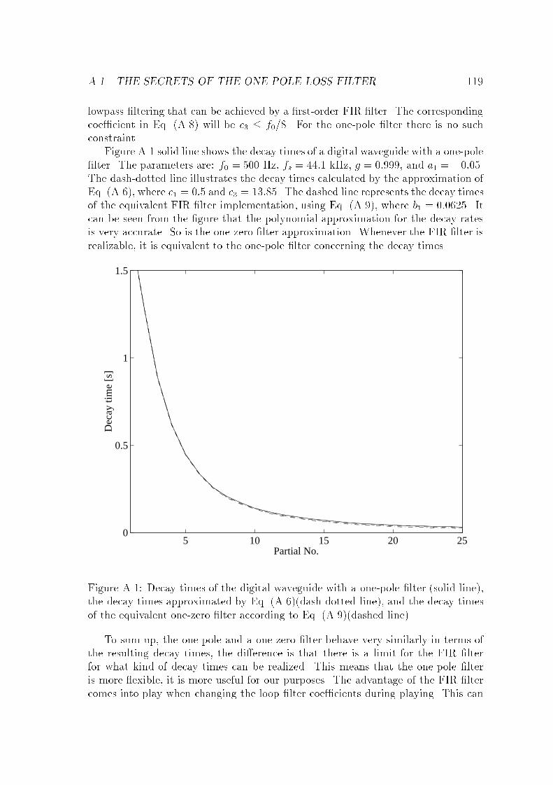
A.1. THE SECRETS OF THE ONE-POLE LOSS FILTER 119

lowpass �ltering that can be achieved by a �rst-order FIR �lter. The correspondingcoe�cient in Eq. (A.8) will be c3 � f0=8. For the one-pole �lter there is no suchconstraint.

Figure A.1 solid line shows the decay times of a digital waveguide with a one-pole�lter. The parameters are: f0 = 500 Hz, fs = 44:1 kHz, g = 0:999, and a1 = �0:05.The dash-dotted line illustrates the decay times calculated by the approximation ofEq. (A.6), where c1 = 0:5 and c3 = 13:85. The dashed line represents the decay timesof the equivalent FIR �lter implementation, using Eq. (A.9), where b1 = 0:0625. Itcan be seen from the �gure that the polynomial approximation for the decay ratesis very accurate. So is the one-zero �lter approximation. Whenever the FIR �lter isrealizable, it is equivalent to the one-pole �lter concerning the decay times.

5 10 15 20 250

0.5

1

1.5

Partial No.

Dec

ay ti

me

[s]

Figure A.1: Decay times of the digital waveguide with a one-pole �lter (solid line),the decay times approximated by Eq. (A.6)(dash-dotted line), and the decay timesof the equivalent one-zero �lter according to Eq. (A.9)(dashed line).

To sum up, the one-pole and a one-zero �lter behave very similarly in terms ofthe resulting decay times, the di�erence is that there is a limit for the FIR �lterfor what kind of decay times can be realized. This means that the one-pole �lteris more �exible, it is more useful for our purposes. The advantage of the FIR �ltercomes into play when changing the loop �lter coe�cients during playing. This can

120 APPENDIX

be the case for the linear damper model in the piano or, more importantly, someother e�ects in other instruments, e.g., in the guitar or in the violin. However, forthose c3 values, which can be still implemented as a FIR �lter, the a1 parameterof the one-pole �lter is small, and so is the transient of the �lter when changingcoe�cients. Consequently, there is no real need for the one-zero implementation.

A.2. MEASUREMENT OF THE PIANO 121

A.2 Measurement of the piano

Measurement characteristics

� The grand piano: August Förster Mod. 170. SN 135178.

� Place: BUTE Schönherz Zoltán dormitory, Budapest, Hungary

� Date: July 21�23, 1999

Measurement equipment

description type sensitivity (EU/V)accelerometer No. 1 PCB 353B13 1966accelerometer No. 2 PCB 353B13 1869microphone TMS13P10/TMS130B10 32.01impact hammer PCB 086C03 4418 channel ampli�er PCB F482A20stereo soundcard Gravis Ultrasound P&Ppersonal computer

Sound card

frequency response 20 Hz � 20 kHz (�3 dB)crosstalk � �50 dBharmonic distortion (THD) � 0:01signal-to-noise ratio (SNR) � 75 dBnominal input level �5 dBVrms

Description of the measurements

The measurement equipment provided the opportunity of two channel measure-ments. The transducers were connected to the input of the multichannel ampli�er.The ampli�ed signals were recorded by a personal computer with a sound card in wavformat. The gain of the ampli�er was set to 10 in all the cases, and the accelerom-eter No. 1 was always used. The only exception was the measurement of hammeracceleration. Then, accelerometer No. 2 was employed, and the corresponding gainfactor of the ampli�er was set to unity.

Accelerometer No. 1 was attached to the bridge by wax. Accelerometer No. 2was �xed on the hammer by the help of thin wire.

The microphone was placed above the string F4 at a distance 12 cm from thesoundboard, and 24 cm from the tuning pins.

The bridge was hit by the impact hammer next to the accelerometer.

122 APPENDIX

Performed measurements

� Examination of the bridge and the soundboard by hitting the bridge with theimpulse hammer

� without sustain pedal (strings damped):

measured parameters: force at the bridge � bridge accelerationforce at the bridge � sound pressurebridge acceleration � sound pressure

measured notes: C1, G1, C2, F]2, C

]3, F

]3, A

]4, G

]5, F

]6, F

]7

number of measurements/note: 20

� with sustain pedal (strings undamped):

measured parameters: force at the bridge � bridge accelerationforce at the bridge � sound pressurebridge acceleration � sound pressure

measured notes: C2, F]3, A

]4, F

]6

number of measurements/note: 20

� Examination of single string vibration with piano hammer excitation (the otherstrings of the doublets and triplets were damped with felt and the una cordapedal was depressed):

� without sustain pedal:

measured parameters: bridge acceleration � sound pressure

measured notes: C1, G1, C2, F]2, C

]3, F

]3, A

]4, G

]5, F

]6, F

]7

number of measurements/note: forte: 5, piano: 5

� with sustain pedal:

measured parameters: bridge acceleration � sound pressure

measured notes: C2, F]3, A

]4, F

]6

number of measurements/note: forte: 3

� Movement of the hammer

� without sustain pedal:

measured parameters: hammer acceleration � bridge acceleration

measured notes: C1, G1, C2, F]2, C

]3, F

]3, C4, A

]4, G

]5, F

]6

number of measurements/note: legato piano: 2, mezzoforte: 2 forte: 2staccato piano: 2, mezzoforte: 2, forte: 2

� Sound of the piano (in natural circumstances)

� without sustain pedal:

measured parameter: sound pressure

measured notes: C1, G1, C2, F]2, C

]3, F

]3, C4, A

]4, G

]5, F

]6, F

]7

number of measurements/note: legato piano: 2, mezzoforte: 2, forte: 2staccato piano: 2, mezzoforte: 2, forte: 2

A.2. MEASUREMENT OF THE PIANO 123

� with sustain pedal:

measured parameter: sound pressure

measured notes: C1, G1, C2, F]2, C

]3, F

]3, C4, A

]4, G

]5, F

]6, F

]7

number of measurements/note: forte: 1