Hierarchical Bayesian Modeling

Angie Wolfgang NSF Postdoctoral Fellow, Penn State

about a population

Making scientific inferences

based on many individuals

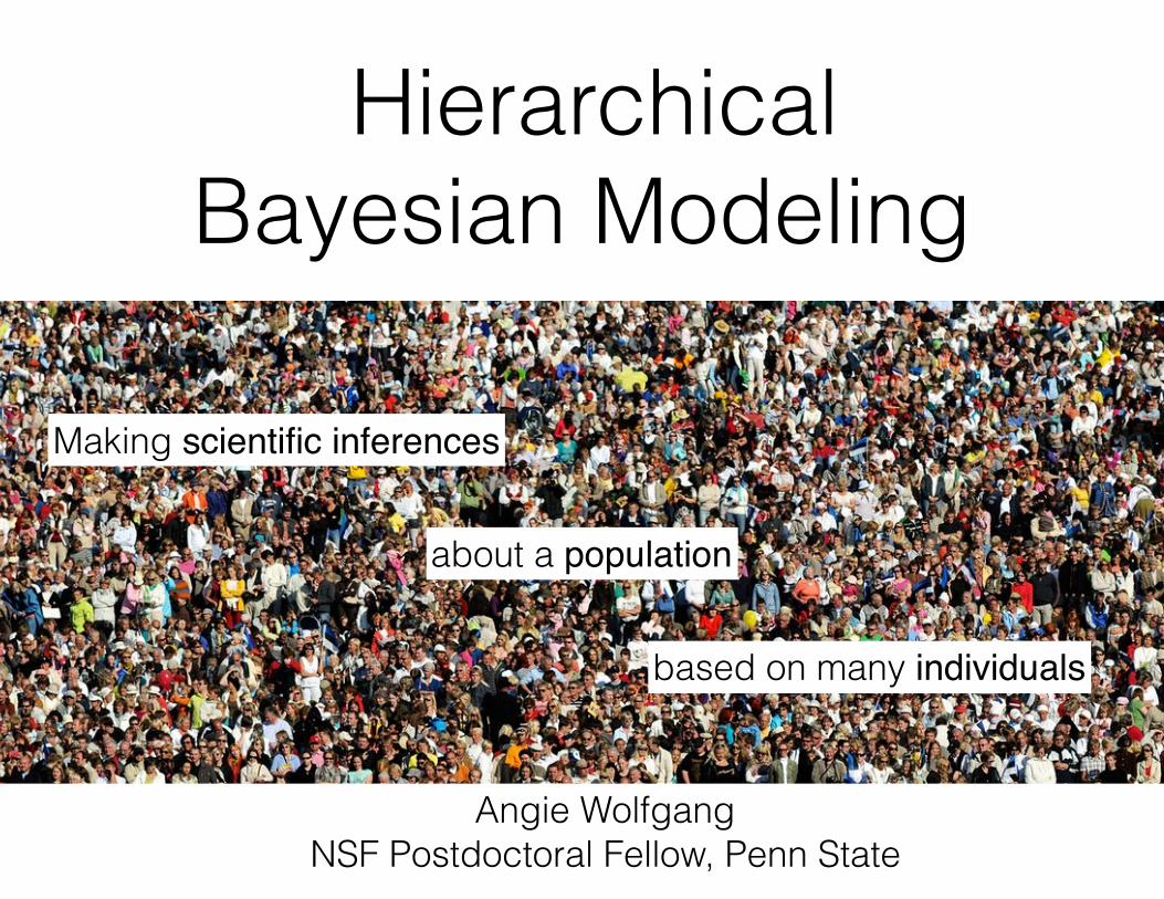
Astronomical Populations

Schawinski et al. 2014Lissauer, Dawson, & Tremaine, 2014

Once we discover an object, we look for more . . .

to characterize their properties and understand their origin.

Kepler planets

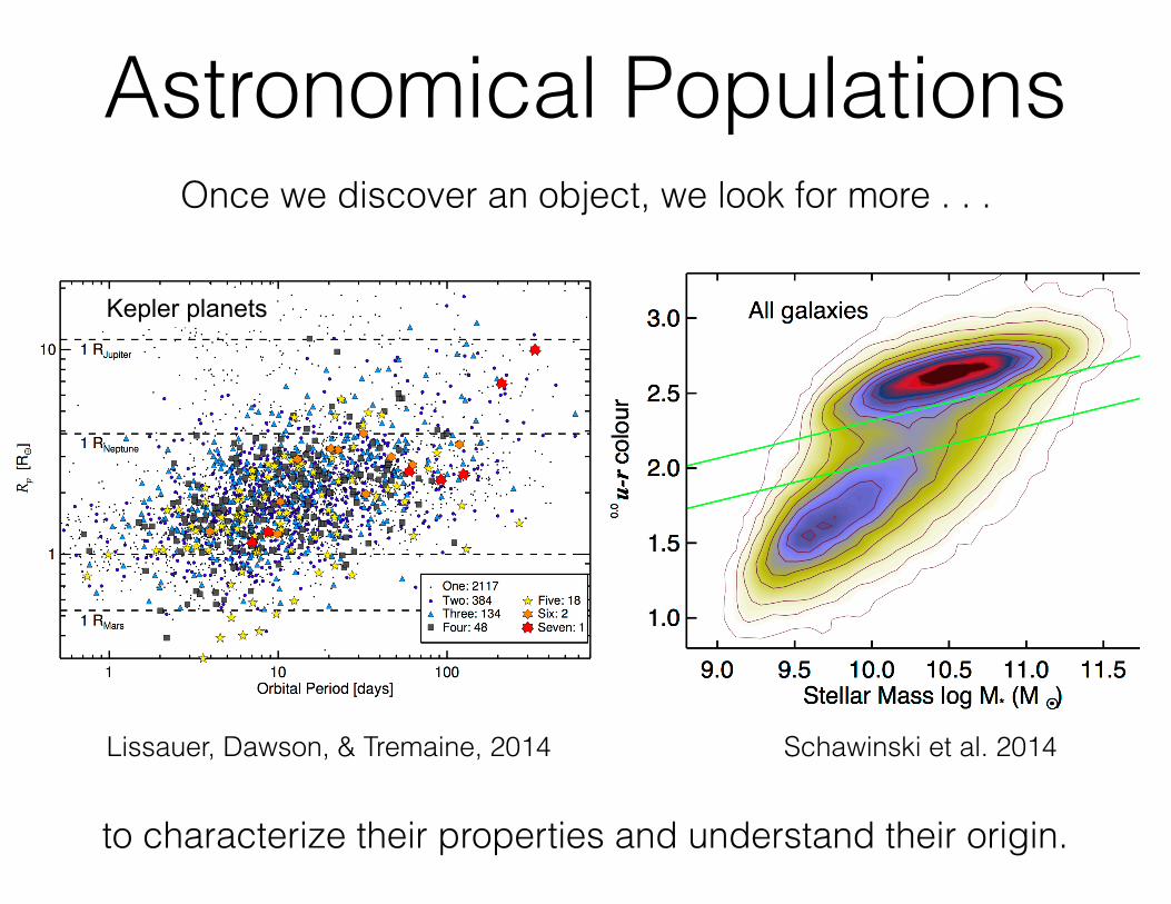
Astronomical PopulationsOr we use many (often noisy) observations of a single object

to gain insight into its physics.

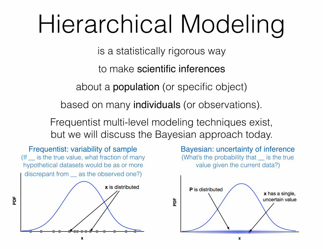
Hierarchical Modelingis a statistically rigorous way to make scientific inferences

about a population (or specific object) based on many individuals (or observations).

Frequentist multi-level modeling techniques exist, but we will discuss the Bayesian approach today.

Frequentist: variability of sample(If __ is the true value, what fraction of many hypothetical datasets would be as or more discrepant from __ as the observed one?)

Bayesian: uncertainty of inference(What’s the probability that __ is the true

value given the current data?)

Understanding Bayes

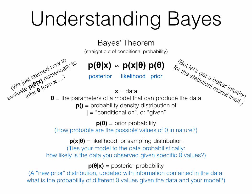
x = data θ = the parameters of a model that can produce the data

p() = probability density distribution of | = “conditional on”, or “given”

p(θ) = prior probability (How probable are the possible values of θ in nature?)

p(x|θ) = likelihood, or sampling distribution (Ties your model to the data probabilistically:

how likely is the data you observed given specific θ values?) p(θ|x) = posterior probability

(A “new prior” distribution, updated with information contained in the data: what is the probability of different θ values given the data and your model?)

Bayes’ Theorem

p(θ|x) ∝ p(x|θ) p(θ)(straight out of conditional probability)

posterior likelihood prior

(We just learned how to

evaluate p(θ|x) numerically to

infer θ from x …)

(But let’s get a better intuition

for the statistical model itself.)

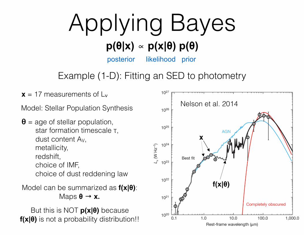
Applying Bayesp(θ|x) ∝ p(x|θ) p(θ)posterior likelihood prior

Example (1-D): Fitting an SED to photometry

x = 17 measurements of Lν

θ = age of stellar population, star formation timescale τ, dust content AV, metallicity, redshift, choice of IMF, choice of dust reddening law

Nelson et al. 2014Model: Stellar Population Synthesis

Model can be summarized as f(x|θ): Maps θ → x.

But this is NOT p(x|θ) because f(x|θ) is not a probability distribution!!

x

f(x|θ)

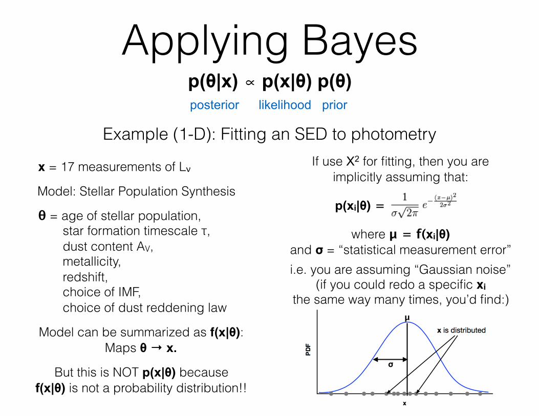
Applying Bayesp(θ|x) ∝ p(x|θ) p(θ)posterior likelihood prior

Example (1-D): Fitting an SED to photometry

x = 17 measurements of Lν

θ = age of stellar population, star formation timescale τ, dust content AV, metallicity, redshift, choice of IMF, choice of dust reddening law

Model: Stellar Population Synthesis

Model can be summarized as f(x|θ): Maps θ → x.

But this is NOT p(x|θ) because f(x|θ) is not a probability distribution!!

If use Χ2 for fitting, then you are implicitly assuming that:

p(xi|θ) =

where μ = f(xi|θ) and σ = “statistical measurement error”i.e. you are assuming “Gaussian noise”

(if you could redo a specific xi the same way many times, you’d find:)

μ

σ

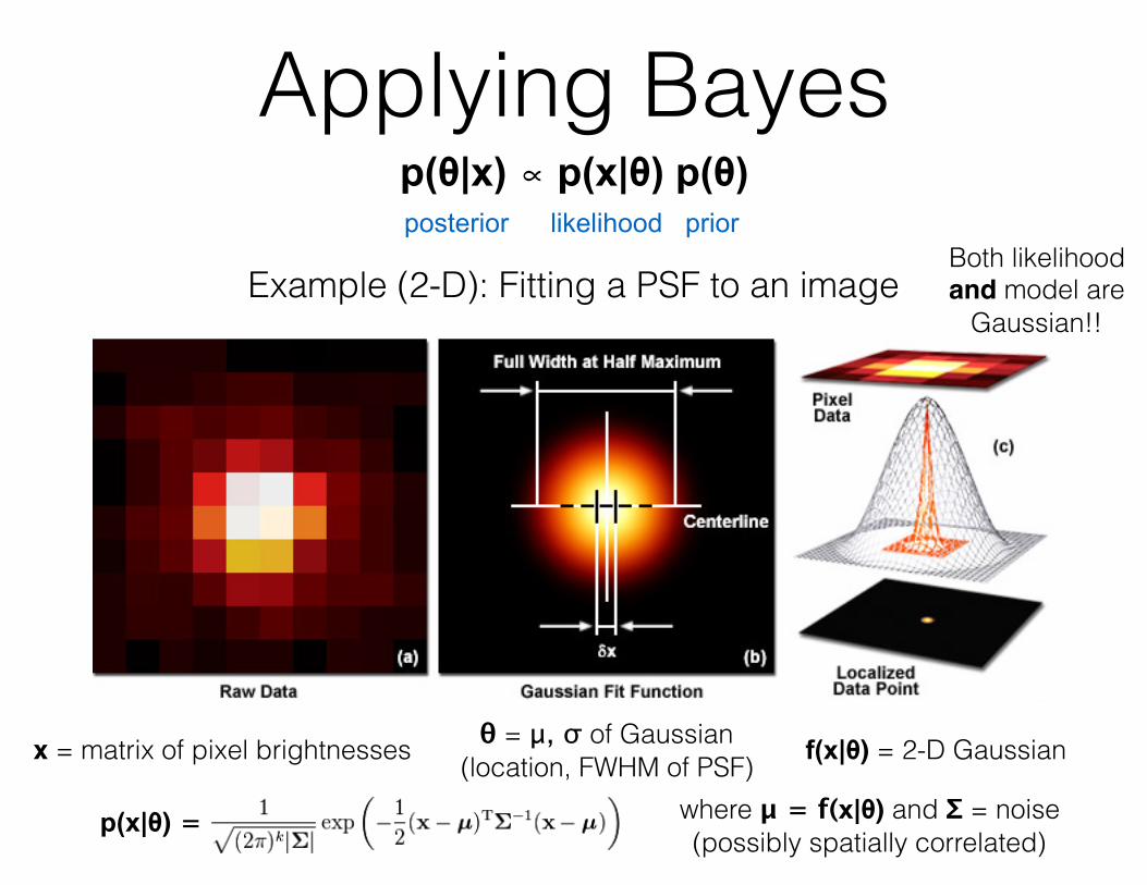
Applying Bayesp(θ|x) ∝ p(x|θ) p(θ)posterior likelihood prior

Example (2-D): Fitting a PSF to an image

x = matrix of pixel brightnesses θ = μ, σ of Gaussian (location, FWHM of PSF) f(x|θ) = 2-D Gaussian

p(x|θ) = where μ = f(x|θ) and Σ = noise (possibly spatially correlated)

Both likelihood and model are

Gaussian!!

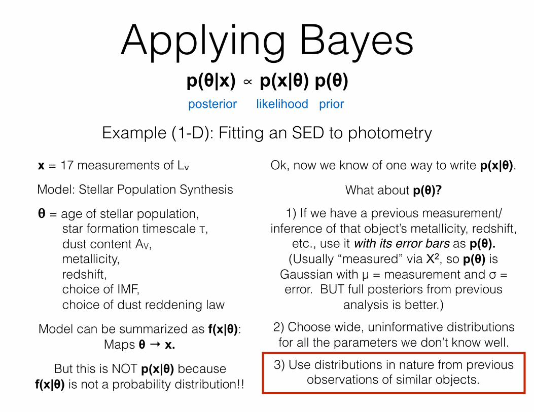
Applying Bayesp(θ|x) ∝ p(x|θ) p(θ)posterior likelihood prior

Example (1-D): Fitting an SED to photometry

x = 17 measurements of Lν

θ = age of stellar population, star formation timescale τ, dust content AV, metallicity, redshift, choice of IMF, choice of dust reddening law

Model: Stellar Population Synthesis

Model can be summarized as f(x|θ): Maps θ → x.

But this is NOT p(x|θ) because f(x|θ) is not a probability distribution!!

Ok, now we know of one way to write p(x|θ).

What about p(θ)?

1) If we have a previous measurement/inference of that object’s metallicity, redshift,

etc., use it with its error bars as p(θ). (Usually “measured” via Χ2, so p(θ) is

Gaussian with μ = measurement and σ = error. BUT full posteriors from previous

analysis is better.) 2) Choose wide, uninformative distributions for all the parameters we don’t know well.

3) Use distributions in nature from previous observations of similar objects.

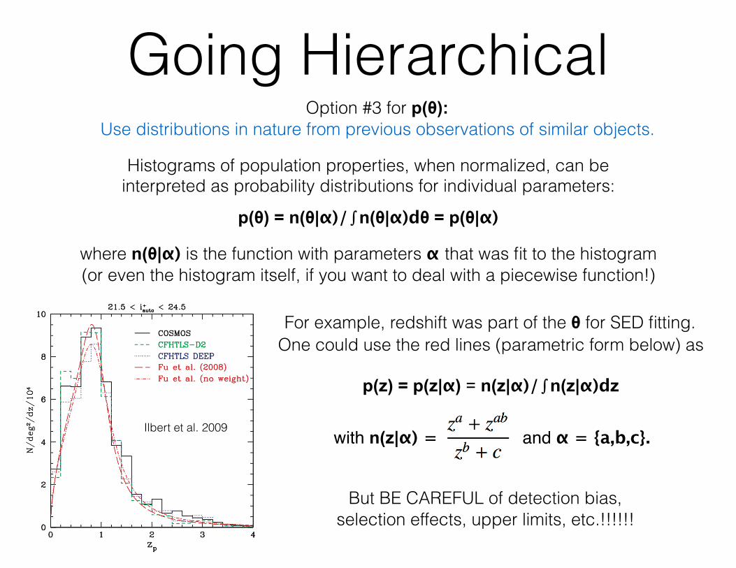
Going HierarchicalOption #3 for p(θ):

Use distributions in nature from previous observations of similar objects.

p(θ) = n(θ|α)/∫n(θ|α)dθ = p(θ|α)

Histograms of population properties, when normalized, can be interpreted as probability distributions for individual parameters:

where n(θ|α) is the function with parameters α that was fit to the histogram (or even the histogram itself, if you want to deal with a piecewise function!)

Ilbert et al. 2009

For example, redshift was part of the θ for SED fitting. One could use the red lines (parametric form below) as

p(z) = p(z|α) = n(z|α)/∫n(z|α)dz

with n(z|α) = and α = {a,b,c}.

But BE CAREFUL of detection bias, selection effects, upper limits, etc.!!!!!!

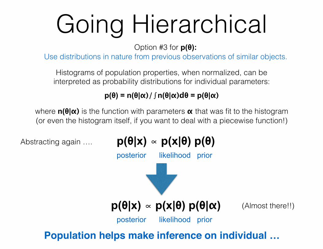
Going HierarchicalOption #3 for p(θ):

Use distributions in nature from previous observations of similar objects.

p(θ) = n(θ|α)/∫n(θ|α)dθ = p(θ|α)

Histograms of population properties, when normalized, can be interpreted as probability distributions for individual parameters:

where n(θ|α) is the function with parameters α that was fit to the histogram (or even the histogram itself, if you want to deal with a piecewise function!)

Population helps make inference on individual …

p(θ|x) ∝ p(x|θ) p(θ)posterior likelihood prior

p(θ|x) ∝ p(x|θ) p(θ|α)posterior likelihood prior

(Almost there!!)

Abstracting again ….

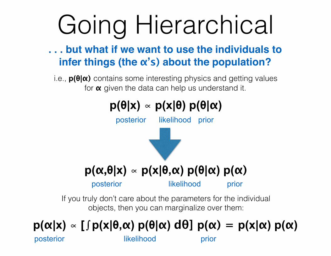
Going Hierarchical. . . but what if we want to use the individuals to

infer things (the α’s) about the population?

p(θ|x) ∝ p(x|θ) p(θ|α)posterior likelihood prior

p(α,θ|x) ∝ p(x|θ,α) p(θ|α) p(α)posterior likelihood prior

If you truly don’t care about the parameters for the individual objects, then you can marginalize over them:

p(α|x) ∝ [∫p(x|θ,α) p(θ|α) dθ] p(α) = p(x|α) p(α)posterior likelihood prior

i.e., p(θ|α) contains some interesting physics and getting values for α given the data can help us understand it.

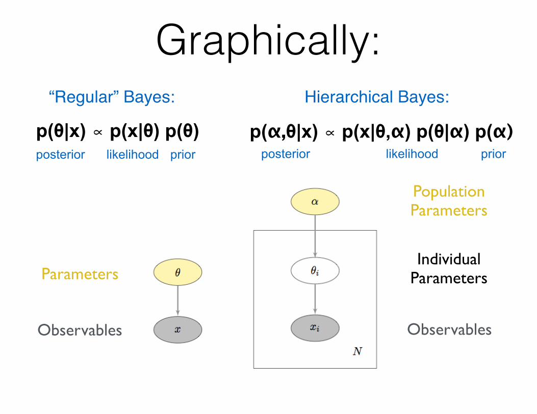
Graphically:

p(θ|x) ∝ p(x|θ) p(θ)posterior likelihood prior

p(α,θ|x) ∝ p(x|θ,α) p(θ|α) p(α)posterior likelihood prior

“Regular” Bayes: Hierarchical Bayes:

Observables

Parameters

PopulationParameters

Observables

Individual Parameters

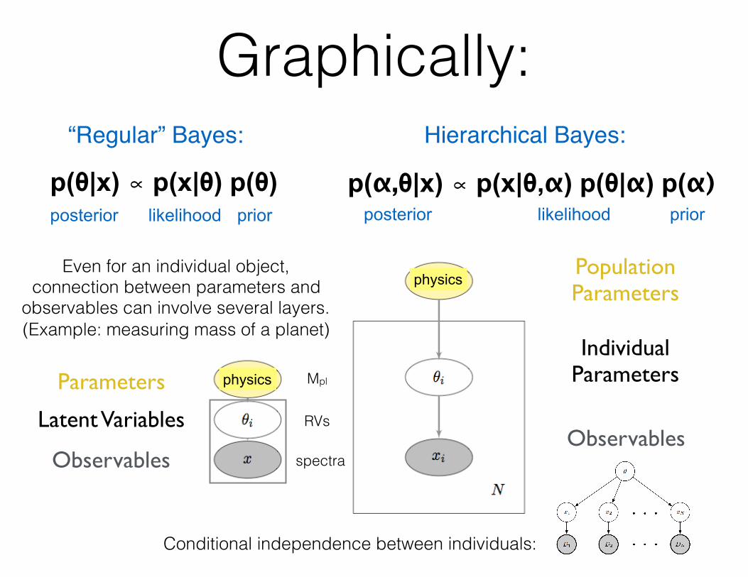
Graphically:

p(θ|x) ∝ p(x|θ) p(θ)posterior likelihood prior

p(α,θ|x) ∝ p(x|θ,α) p(θ|α) p(α)posterior likelihood prior

“Regular” Bayes: Hierarchical Bayes:

Observables

Parameters

PopulationParameters

Observables

Individual Parameters

physics

physics

Conditional independence between individuals:

Even for an individual object, connection between parameters and

observables can involve several layers. (Example: measuring mass of a planet)

Latent Variables

Mpl

RVs

spectra

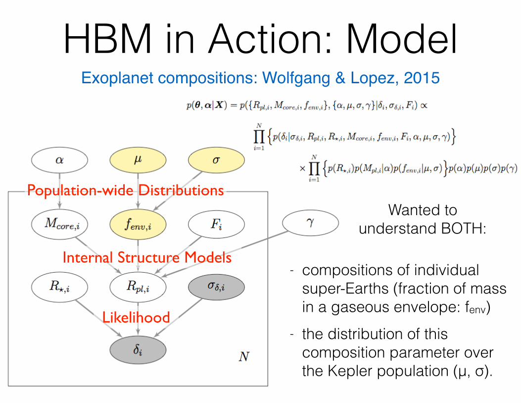
HBM in Action: Model

- compositions of individual super-Earths (fraction of mass in a gaseous envelope: fenv)

- the distribution of this composition parameter over the Kepler population (μ, σ).

Internal Structure Models

Population-wide Distributions

Likelihood

Wanted to understand BOTH:

Exoplanet compositions: Wolfgang & Lopez, 2015

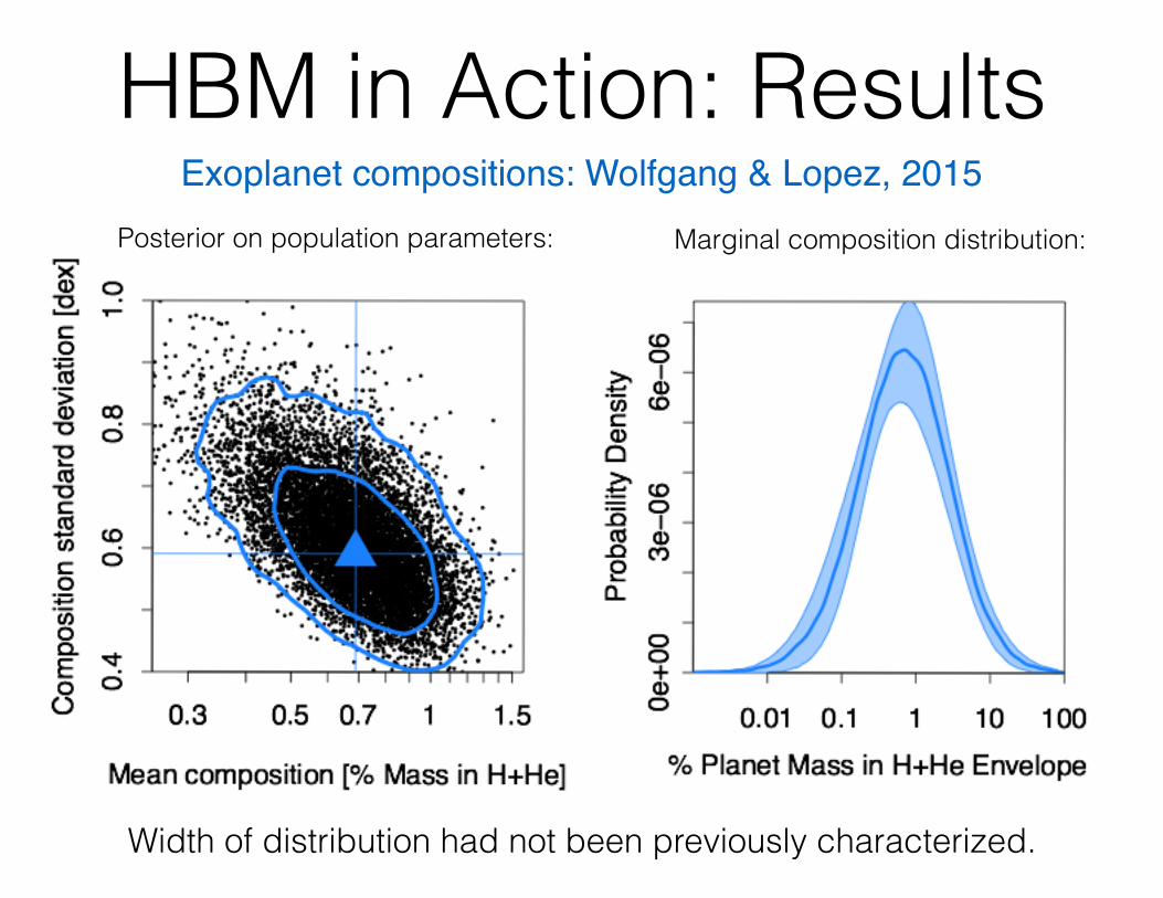
HBM in Action: ResultsExoplanet compositions: Wolfgang & Lopez, 2015

Posterior on population parameters: Marginal composition distribution:

Width of distribution had not been previously characterized.

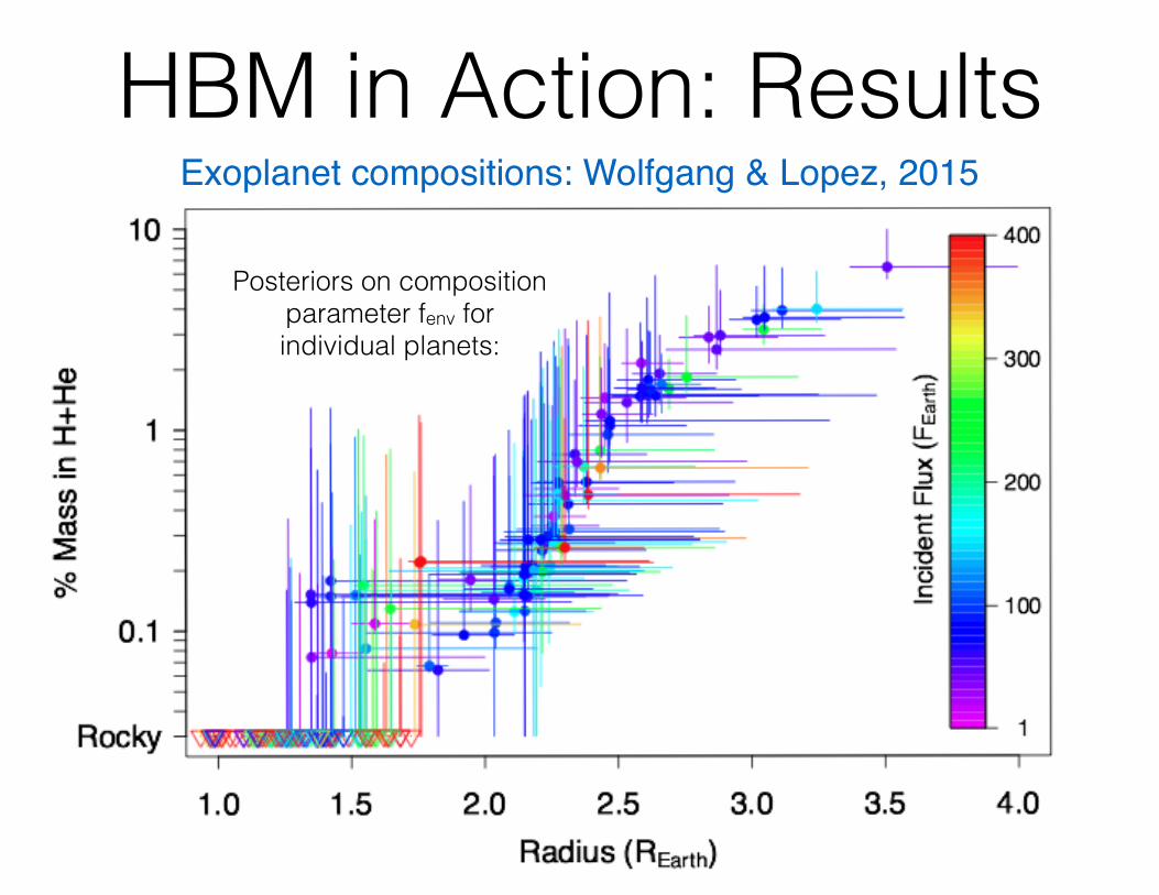
HBM in Action: ResultsExoplanet compositions: Wolfgang & Lopez, 2015

Posteriors on composition parameter fenv for individual planets:

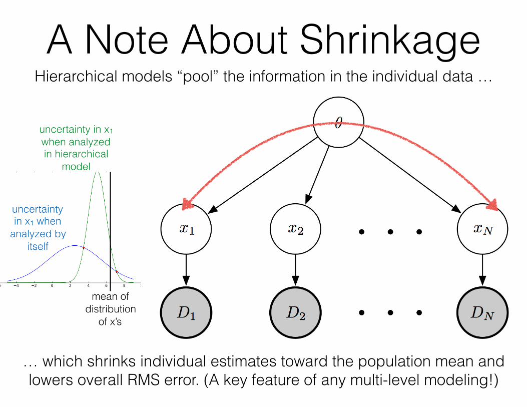
A Note About ShrinkageHierarchical models “pool” the information in the individual data …

mean of distribution

of x’s

uncertainty in x1 when

analyzed by itself

… which shrinks individual estimates toward the population mean and lowers overall RMS error. (A key feature of any multi-level modeling!)

uncertainty in x1 when analyzed in hierarchical

model

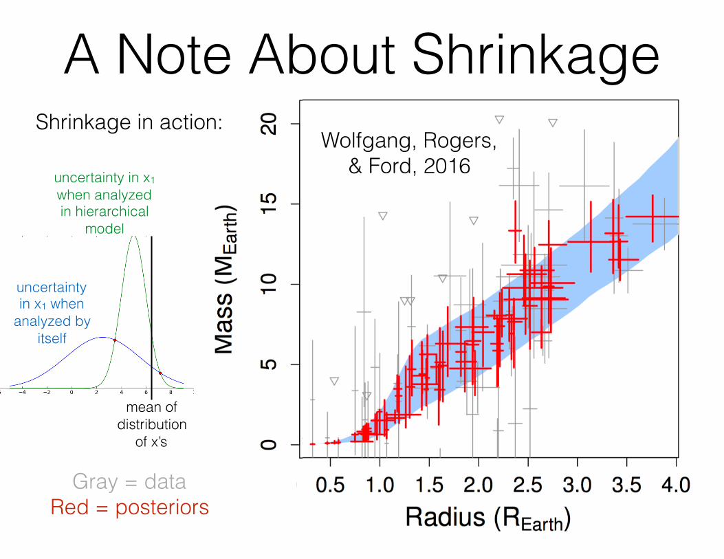
A Note About Shrinkage

mean of distribution

of x’s

uncertainty in x1 when analyzed in hierarchical

model

uncertainty in x1 when

analyzed by itself

Wolfgang, Rogers, & Ford, 2016

Shrinkage in action:

Gray = data Red = posteriors

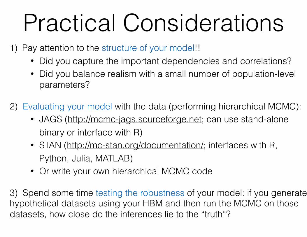
Practical Considerations1) Pay attention to the structure of your model!!

• Did you capture the important dependencies and correlations? • Did you balance realism with a small number of population-level

parameters?

2) Evaluating your model with the data (performing hierarchical MCMC): • JAGS (http://mcmc-jags.sourceforge.net; can use stand-alone

binary or interface with R) • STAN (http://mc-stan.org/documentation/; interfaces with R,

Python, Julia, MATLAB) • Or write your own hierarchical MCMC code

3) Spend some time testing the robustness of your model: if you generate hypothetical datasets using your HBM and then run the MCMC on those datasets, how close do the inferences lie to the “truth”?

In Sum, Why HBM?• Obtain simultaneous posteriors on individual and population parameters: self-consistent constraints on the physics

• Readily quantify uncertainty in those parameters

• Naturally deals with large measurement uncertainties and upper limits (censoring)

• Similarly, can account for selection effects *within* the model, simultaneously with the inference

• Enables direct, probabilistic relationships between theory and observations

• Framework for model comparison

Further Reading

DeGroot & Schervish, Probability and Statistics

(Solid fundamentals)

Gelman, Carlin, Stern, & Rubin, Bayesian Data Analysis (In-depth; advanced topics)

Loredo 2013; arXiv:1208.3036 (Few-page intro/overview of multi-level

modeling in astronomy)

B.C. Kelly 2007 (HBM for linear regression, also applied

to quasars)

Loredo & Wasserman, 1998 (Multi-level model for luminosity distribution of

gamma ray bursts)

Mandel et al. 2009 (HBM for Supernovae)

Hogg et al. 2010 (HBM with importance sampling for exoplanet

eccentricities)

Andreon & Hurn, 2010 (HBM for galaxy clusters)

Martinez 2015 (HBM for Milky Way satellites)

Wolfgang, Rogers, & Ford 2016 (HBM for exoplanet mass-radius relationship)

Introductory/General: Some applications: