SAC-PUB-45 August 1964

HIGH ENERGY y RAY SOURCE FROM ELECTRON POSITRON PAIR ANNIHILATION*

Yung-Su Tsai

Stanford Linear Accelerator Center Stanford University, Stanford, California

ABSTRACT

Problems associated with using the process e+ + e- i2y as

a source for high energy y ray are investigated. The polari za-

tion of the y's is shown to be negligible at high energies. The

spread of y spectra at a fixed angle due to radiative corrections

is investigated. It was found that terms like : <a" k$ are as-

sociated with infrared divergence and disappear with a reasonable

energy resolution. The result obtained is found to be very similar

to Schwinger's corrections without vacuuII1 polarization. Our result.

was found to be also usable in the colliding beam experiment without

any modification under certain conditions.

(To,be submitted to Physical Review)

* Work supported by U. S. Atomic Energy Commission.

-l-

In the usual eqertients involving photons ee incident particles, the.

photon source is from the ordinary bremsstrshlungs which are not only non-

monochromatic but also strongly dominated by low energy' 7's due to the

l/k dependence in the bremsstrahlunq crqss sections. This fact not only

imposes some complications to the kinemat," <pal analysis of the subsequent

photopo&ction prep. ysses but also swetimes renders the experiments impos-

sible due to the enormous background Produced by the, low ener&y‘ 7'6; fop

example in the bubble chamber expriments the= will be too many camPton

electrons and electron pairs produced. Ballam and Guiragossi&' made a pro-

posal to use the fact that when positrons are injected into the hydrogen

target one obtains monochromatic Y's from e4 + e- -27 process in ad-

dition to the ordinary bremsstrahlung from e+ + e- --+e+ + e- 4 7' and 4 4 e f p -+e +p+r. One hopes that the y's thus produced will have

sufficiently high energy ccmponents to overcome part of' the difficulties

mentioned abava. fn order to obtain a resultant gamma spectra from ef

hydrogen atw colLision one has to calculate the follcrwiqg four processes

in detail:

1. e+ + e- -+2y and Its radiative corrections

2. e+ + e- 43y '

3. e*+e--+e++e-+7

4, e+ +p-+e++p+r

In this paper we treat only the 1st process and part of the second process

where the third photon emitted is ltiited to a low energy. The exact treatments

-2-

I

of process 2, 3 and 4 can be done by an electronic computer and will be pub-

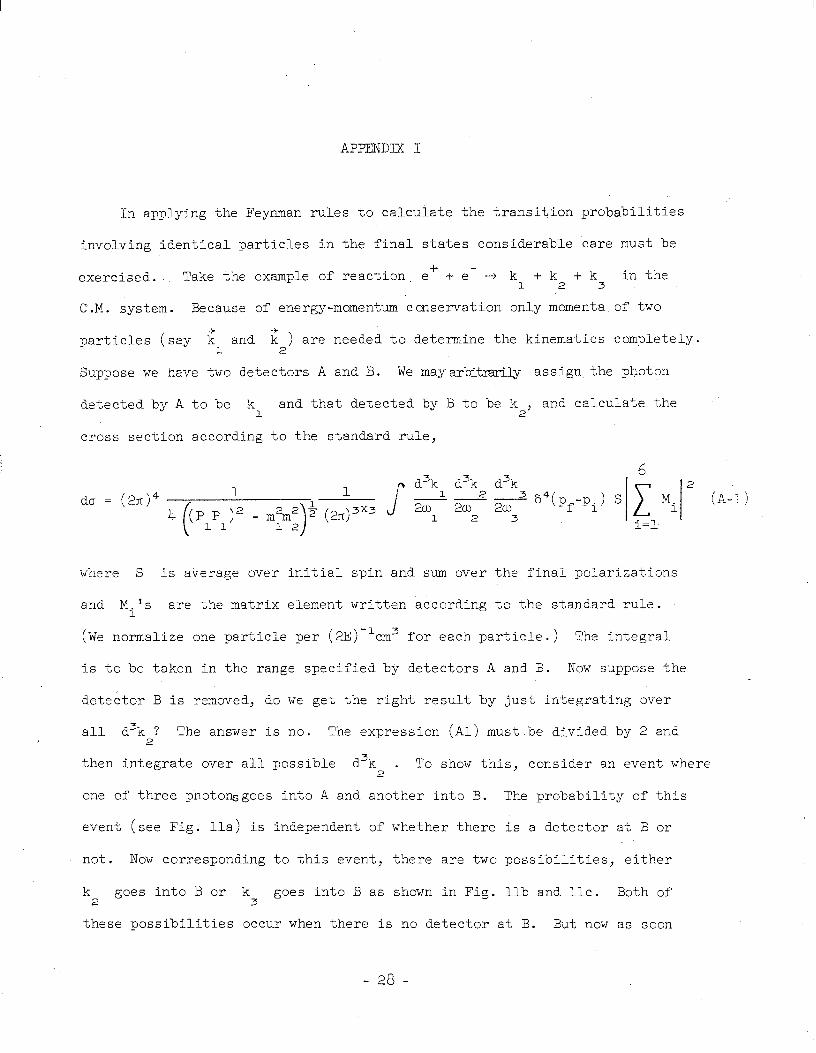
lished separately.2 Figure 1 shows the anticipated 7 spectrum at a fixed

angle. The spike in the figure is due to process 1 and 2. The processes 2,

3 and 4 contribute to the smooth curve in the background. The troublesome

low energy end of the spectrum can usually be greatly reduced by passing the

7 rays through some material using the fact that the absorption coefficient

for the low energy 7 rays is larger than that for the high energy 7 rays.

In Section 2, we treat the lowest order process, define the notations,

give many useful kinematical relations.and formulae and show that the polari- +

zation of the 7 rays produced in the process e + e- + 27 is negligibly

small at high energies. In Section 3 the spreading of the y spectra due

to radiative corrections is calculated. It was found that the terms like

do not occur in our final expression for the radiative corrections

6 . It is concluded that terms like are closely related to the

infrared phenomena and disappear when the phase space for the third photon

k3 is taken to be such that max CL! >> m in the center of mass system. (See 3

Section 5.) In Section 4 some numerical examples are given. In Section _5,

the Fhysical significance of existence or absence of terms like (92%

is discussed. The resemblance .between our results and Schwinger's formula

is pointed out, and finally the adaption of our result to the colliding. beam

experiment is considered. In the Appendix we discuss some precautions needed

in the calculation of cross sections involving many identical particles in

the final states.

-3-

2. e+ + e- -+2y

In this section we treat the lowest order cross section. Since we are

interested only in the very high energy + e beam we may treat the electron

in the hydrogen atom to be free. P and P 1 2 represent the four momenta of

the target electron and the incident positron respectively. ki and el

represent the four momenta and polarization vector of the detected photon

and k and e Quantities with 2 2

represent those of the undetected photon.

a bar on top represent the center of mass quantities. Our metric is defired

such that if k = 1

The units used are

laboratory system

e; G

( pl

=a, and ?S='c =l. We choose a gauge such that in the

e;P1 = e;Pi = 0 and e .k = e Sk2 = o. By 11 2

calculating the lowest

the differential cross

order Feynman diagrams shown in Fig. 2, one obtains

section

r 1

du r2 w o (e ,e,) = o

m2 (m t- E2)

1

$ + a2 f 2 - 4 (el-e2j2 . . . I d.Qk 1 8

k-1) P2 (m + E - P2~~s@)2 2 1

2 -!

where r: = 7.93 X 1O-26 cm2 and 8 is the angle between "p2 and k . -1

For convenience in discussing the polarization, let us choose a coordinate

in which the direction of .k , is the z -1 axis and that of Al X k --2

is the y

axis as shown in Fig. 3. Then the summation over e can be carried out with 2

respect to two transverse directions

e 3 (0, f case 2fl 12’

0) - sine ) 12

-4-

and the result is

“2 +rt2-2 e2 C

cos20 + e 1X 12 1

(2-2)

where

2 m2 (m + E2)

P2 (m + E2 - P2 ~0~0)~

From Eq. (2-2) we can construct the density matrix for the photon beam k 1'

(z-3)

where i = x, y and j = x, 7y.

The density matrix X completely specifies the quantum mechanical descrip-

tion of a monochromatic photon beam kl because any subsequent interaction of

k can be written as Tr MXM+ where M is the matrix element of the sub-

szquent interaction. (P rovided one uses the same gauge as used here.)

However it is more convenient to give an equivalent description in terms of

intensity of the beam and the three Stokes parameters Sx, S , Y and Sz.

The trace of X gives'the differential cross section summed over the

polarization e- and is given by

daO u!

-=TrX=A d'k

i 0

2 2 f 2 1

-t sin28 12

1

(2-4)

-5 -

I

The definitions of the Stokes parameters, their functional form of our par-

titular problem and their physical meanings can be given by the following

equations.3 (See Fig. 4.)

sx = Tr oxX X x +Xx

Trx = Tr x Lo.

Tr aX s =+=

Y Tr X = 0

(2-6)

da =-

da

i 2 -1 A ( Sl

i A %L

c $

1

Tr ozX Xxx - X sin20 sz= TrX = TrX =LU u)

12

$- + 2 + sin28 12

1 (T-7)

- 6 -

It is seen that the only nonvarnishing Stokes parameter is S and Z

Eq. (2-7) shows that there are more photons plane polarized in the produc-

tion plane (x-z plane) than those perpendicular to the production plane.

The magnitude of Sz is roughly proportional to f32 12 '

the square of the

angle between two photons produced. The differential cross section and the

only nonvarnishing Stokes parameter Sz 'of Eqs. (2-4) and (2-7) can be

written in terms of 8 and E alone 2

by the following kinematic relations.

(E2 + m) m

u! = 1 m+E

2 - p2c0se

E x

1 +2g ' (2-8)

(E2 + m) (E - P2cosB) Ey82 03 2 2 2 = =

2 m+E PacosB -l+g' (2-P)

- 2

2(E - m) sin28 sin% = 2

12 E 2

- P2cosB

The approximate relations x hold only when

1 >> 8 >>

Hereafter we use the symbol y to represent approximate relations true

L

(E2 - m)2sin4e

(E,, - y0se j2

m-l -=- E Y'

2

4 z-c=zo y2e2

(2-11)

only if inequalities Eq. (2-11) are satisfied.

- 7 -

men 1 >> 8 and y >> 1 we may write"

duo rg d.Ok = ?-

+ 4yW

1 + y2e2 (2-12)

(2-13)

The second relation holds only when inequalities Eq. (2-11) are satisfied.

Similarly for Sz we have

sz = 8e2y

(4 + y2e4) (1 + y2e2) (2-14;

For convenience of order of magnitude estimate we give some of the values

of dci/dRk and S in Table I. 1 Z

TABLE I

8 da

d% L

sZ

0

1 Y J- - 1 v r

rzy

$7 2

0

1 r

8 5

-8-

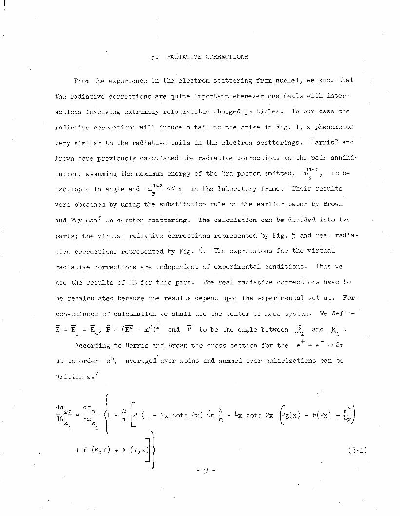
3. RADIATIVE CORRECTIONS

From the experience in the electron scattering from nuclei, we know that

the radiative corrections are quite important whenever one deals with inter-

actions involving extremely relativistic charged particles. In our case the

radiative corrections will induce a tailto the spike in Fig. 1, a phenomenon

very similar to the radiative tails in the electron scatterings. Harris? and

Brown have previously calculated the radiative corrections to the pair annihi-

lation, assuming the maximum energy of the 3rd photon emitted, max, to be

isotropic in angle and w max << m in the laboratory frame. Their results 3

were obtained by using the substitution rule on the earlier pa-per by Brown

and Feynman6 on compton scattering. The calculation can be divided into two

parts; the virtual radiative corrections represented by Fig..5 and real radia-

tive corrections represented by Fig. 6. The expressions for the virtual

radiative corrections are independent of experimental conditions. Thus we

use the results of HB for this part. The real radiative corrections have to

be recalculated because the results depend upon the experimental set up. For

convenience of calculation we shall use the center of mass system. We define

E = z 1

- =E

2’ p= (E2

.L m2)2 and s to be the angle between F .-, 2

and ‘i; _ . . 1

According to Harris and Brown the cross section for the ef + e- 32~

up to order e6, averaged over spins and summed over polarizations can be

written as 7

da daO 2r=----

dL-Lk dSlk 1 1

+ F (K.,T) + F (7,~)

?

- h(2x) +

(3-O

where A is the usual fictitious photon mass and

T’ - 2~ + KIT

2K2!7 (K - 1)

The symbols used in the above equations have the following meaning:

2P ok 2P Sk TE 1 2= 2 1

2 m m 2 :’

42 2- K+T=----= 4T2 ,

rl?

- 10 -

-II- cash x = y = : ’

u= 4 (+++)’ - 4 ($+$) - ($;) ,

X

s u tanh u du ,

0

X

h(x) = $ s

ucothudu ,

0

and l.-‘c

Go(x) = E s

h-l (l-u) $ *

1

We not ice that if the inequalities (2-11) hold, then

7 >> 7 >> 1

and

(3-3a)

K >> 7 >> 1 . (3-3b)

Since the definitions given above by HB are unwieldy we give simplified

(but exact) expressions as well as approximate expressions which hold only

when (2-11) is satisfied.

sinh x = - x m 7 Y

- 11 -

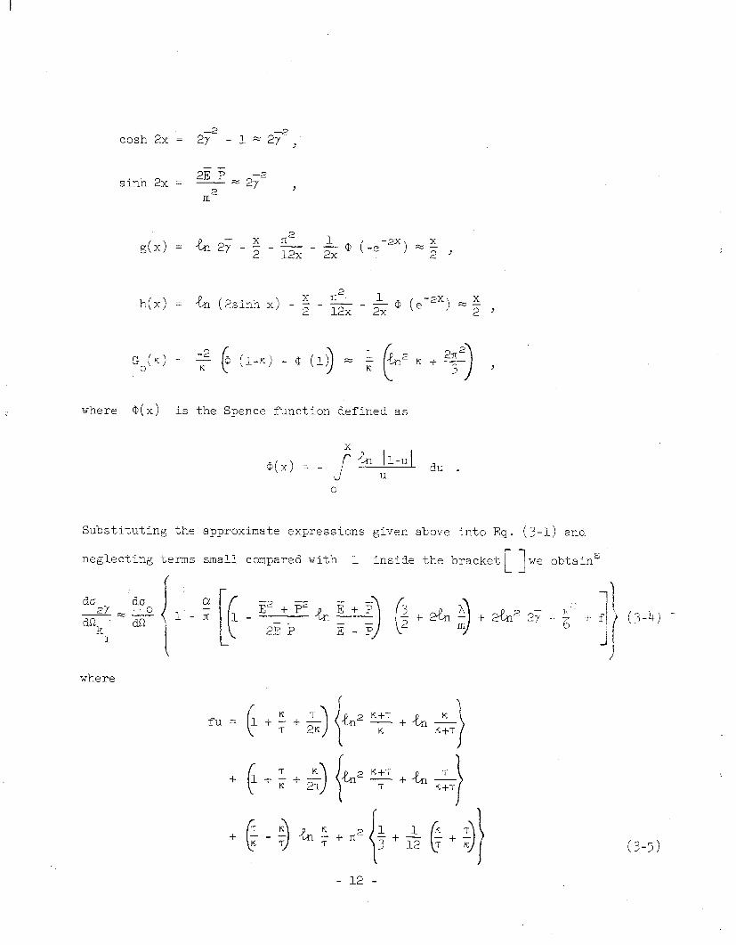
cash 2x = 2r2 - 1 = 2y2,

sinh 2x = 2E F ~ 2

s2 , m

h(x) = & (2sinh x) - z - & - & Q (emzx) z g ,

Go(") = $ 6 (1-K) - G ,

where Q(x) is the Spence function defined as

0

Substituting the approximate expressions given above into Eq. (3-l) and

neglecting terms small compared with 1 inside the bracket tl we obtain'

where

(3-5)

We next calculate the cross section for e+ + e- -+3?'. In principle one

could calculate this cross section exactly by going into the center of mass

system of two undetected particles as was done in other three particle final

state problems. ' We shall not calculate this cross section exactly here but

merely try to find the dominant terms (such as log y, %I y -fin & etc.), 1

because these. terms can be obtained without much effort and one expects that

the resultant formula should be accurate to within one or two percent which

is hopefully quite sufficient for the experimentalists needs. We shall cal-

culate everything in the center of mass system. lo To do this we have to specify

what we are looking for in the laboratory system and then transform the lab

experimental conditions into those of the C.M. We are interested in the

photon spectra at a certain angle in the lab system. We anticipate the spec-

trum will look like what is shown in Fig. 7. (The photons due to ordinary

bremsstrahlung have been substracted already.) Usually the incident positron

energy E and the angle 8 have certain width LX3 and A@ and they cause 2 2

the width W to the right of the peak in the spectrum. In the vicinity of

the peak the shape of the spectrum is dominated by ma and 40 and has very

little to do with the radiative corrections. What one can calculate by using -

the standard method is the area under the curve between mLn *and c as a

function of &D1 as shown in Fig. 7 provided Cro 1 is large compared with W.

Even if in the ideal case where W is infinitly small AL should not be 1 taken too small'i because of the infrared divergence difficulties inherent in

the perturbation method. Since the area as a function of AJJ can'be cal- l culated, we can obtain the spectrum itself in the region where &r >> w by

1 simply differentiating the expression for the area with respect to AJ . 1

- 13 -

Thus our experimental condition in the lab frame can be stated as llHow many

photons can be detected in a small angular range 46 with energy u)~ > ayl"

if the incident positrons have energy E2 ?" In the center of mass system

we have incident positron energy

the scattering angle S

and the energy of the detected photon

From the above equations we can construct the phase space for the photon

k 1 -in the center of mass system represented by an area ABCI)

The horizontal line AB is obtained by setting G :. E where 1 2

by Eq. (3-6). 8 min is obtained from Eq. (3-T), max

'%in l- case = max

min . max 'YZn max 1+7

(3-6)

.n Fig. 8.

E 2

is given

(3-9)

- 14 -

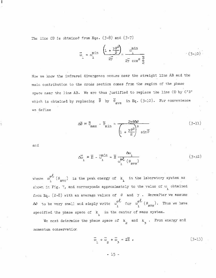
The line CD is obtained from Eqs. (3-8) and (3-7)

cumin min 1 cu =W =

1 1 21 27 cos 23 2

(3-10) ‘.

Now we know the infrared divergence occurs near the straight line AB and the

main contribution to the cross section comes from the region of the phase

space near the line AB. We are thus justified to replace the line CD by C'D'

which is obtained by replacing s by gave in Eq. (j-10). For convenience

we define

As t 3 -3 zz 2yem max min 2

sins

and

(3-11)

(3-12)

where cu f ('ave) is the peak energy of k in the laboratory system as 1

shown in Fig. 7, and corresponds approximately to the value of CD obtained 1

from Eq. (2-8) with an average values of 63 and y . Hereafter we assume

e-L LI6 to be very small and simply write u)~ for UT' (cave). Thus we have

specified the phase space of k in the center of mass system. 1

We next determine the phase space of k2 and k3 . From energy, and

momentum conservation

cu fW +co = 2E , 1 2 3

(3-13)

- 15 -

and kl+E +k =o,

2 3 - - Lu (3-14)

we can show that for each value of E the allowed values of k and -2 2.

iT must be on the surface of an ellipsoid with k vector connecting 3 1 -

the two foci as shown in Fig. 9. The ellipsoid shrinks to a line when - -min w = E and.has a maximum extension when w = (0 Thus the phase space

1 1 1'

of k and k can be represented by all the points inside the ellipsoid 2 3

obtained by setting G -min =(u . and k 1 1

In principle one has to treat k 2 3

symmetrically since they are identical particles and both are undetected.

However as is shown in the Appendix we need to consider only half of the

phase space, Fig. 10, due to the symmetry between k and k . In this 2 3

phase space only X3 but not k2 can become infrared. The distance from

the point o to any point on the surface of this semiellipsoid gives the

maximum value of cu , and is a function of angle 3

(z13) between ki and

k 3

in the center of mass system. Explicitly one obtaines

-- 2Edw

;;;"a" z. 1 3

E + Gl + (E-&q case 7

13

for

(3-15a)

and

E-&i ii- = - 1

3 2cos-G >

13

(3-15b)

- 16 -

I

for

Equation (3-15a) represents the equation for the ellipsoid and

Equation (3-lpb) represents the bottom flat surface in Fig. 10. Some

s-implification to the phase space of k can be obtained by explicitly 3

considering the nature of the matrix elements.

There are 6 diagrams which contribute to the 3y annihilation process

as shown in Fig. 6. k3 is not connected to the external charged lines in

M and M and thus M and M are not infrared divergent as can be 5 6 5 6

verified by explicit calculations. For simplicity of the calculation we

shall ignore M and M and further the terms proportional to k in the 5 6 3

numerator. l2 Then the cross section for 3y annihilation can be written as

- - du

3Y - do0 a ---- d.Q di-2 s JTs - (P1$P2k3) + (P;:3)2

>

(3-16)

In the center of mass system both Pl and P are extremely relativistic 2

and the denominators in the integrand of Eq. (3-16) tell us that practically

all k are emitted either along p or p Thus we expect the result 3 1 2' -

of the integration is quite insensitive to the detail shape of the phase

space except in the vicinity of k3 // p and k3 // F2 . The maximum values

of w along P and P can bFobta<ed from<qs.T3-15a,b) by setting 3 1 2

- 17 -

3 = fl - 3 and s = S respectively, and are to be denoted as 13 13

cu y" (k #P > and "c3 -1 zy" (k

-3 //z ) respectively. We have tacitly assumed

2

that E is much smaller compared with z in order to obtain a very simple 3

expression (Eq. 3-16) for the 3y annihilation cross section. But from z

Fig. 10 we see that even for small &l ., G3 can be as large as N 2 .

However, as can be seen from Eq. (3-15) and Fig. 11, if

both myx (",/&) are always small compared with

z if LG is small. Hence we shall assume that inequalities (3-17) are 2 1

satisfied.13 The integration (3-16) is a familiar one occurring in every

bremsstrahlung calculation. Past experiences14 show that the phase space

shown in Fig. 10 can be replaced by a sphere with a radius c ax defined

by a geometrical mean

= 2E L4.i 1 [(E +,LG,)’ ( E - &l)2 1

-- : cos2e . Carrying out the integration in this spherical phase space, and neg-

lecting non-logarithmic terms, we obtain15

(3-18)

- 18 -

where K(Pi, Pj ) is the infrared terms and defined by

K(Pi,Pj) = (PiPj) &s- dx (3-20) i 0 pz

with Px = PiX + Pj(l-x). It was emphasized by the author in previous worksg'1o

that it is a good idea not to integrate terms like K(Pi,Pj) explicitly

because they always cancel between elastic and inelastic radiative corrections.

However, since we are going to use Harris and Brown's results on the elastic

part we give the explicit expressions'for K(Pi,Pj) in the center of mass

system. (Of course the expression can be covariantized easily.)

K(Pl,Pl) = K(P2,',) = &n y . (3-21)

(3-22)

(3-23)

Experimentally meaningful cross section can be obtained by adding Eq. (j-19)

- 19 -

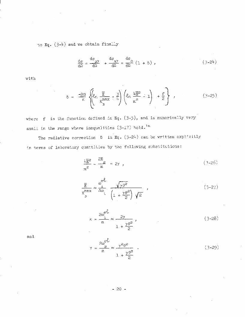
to Eq. (3-4) and we obtain finally

da a0 __

aa aa 2Y

-= ai2 3Y _

all + - - $ (l+ s) , a!2

with

where f is the function defined in Eq. (3-5), and is numerically very

small in the range where inequalities (3-17) hold.16

The radiative correction 6 in Eq. (3-24) can be written explicitly

in terms of labora.tory quantities by the following substitutions:

and

et 2!u, 1 K _-x 27

m

- 20 -

(3-24)

(3-26)

( 3-27)

(3-28)

(3-29)

In summary, Eq. (3-24) gives the area under the curve of Fig. 7 from min (0 1 to c as a function of &i in the range

CL+ 1

O.l>hu >w, 1 (3-30)

(3-31)

The lower limit of nL0 in (3-30) is necessary because near the peak in Fig. 7, 1

the shape of the spectra is mainly determined by &X2 and A@ and further

even if LYE and 5f3 were zero (i.e. Go), 41.! should not be taken too 2 1

small because of infrared divergence difficulties, i.e. Eq. ('3-24) diverges

as AX 30. A proper criteria to ascertain that we are not in the infrared 1

region is that L&U 1

should be taken large enough such that17 .-6 5 0.2. On

the other hand the upper limit of L"ro 1

and inequalities (3-31) were imposed

because we had assumed (I, 3 to be small compared with E in order to obtain

Eq. (3-16). Inequalities (3-31) are merely the reexpression of the C.M. con-

dition (3-17) in terms of lab quantities.

Differentiating Eq. (j-24) with respect to nLu we obtain the spectral 1

distribution of w 1 at angle 8 in the lab system,

(3-32)

which is correct only if cyu =aee-e-, and 8 are such that (3-30) and 1 1 1

(3-31) are satisfied.

- 21 -

4. NUMERICAL EXAMPLES

In order to facilitate numerical computations we shall rewrite all our

formulae in more compact forms. We are mainly interested in the regions of

6 and hu specified by inequalities (2-U)' (3-30) and (3-31). Let us 1

introduce two new symbols

z -‘Ye2 2 (4-l)

& cl.! RZ----

2 (4-2)

1

The lowest order cross section for e+ t e- -+2y can be written as

(see Eq. 2-13)

aoo r: 1 '1 q

zz- 2 (1+z)2 z + z - ( )

The radiative corrections 6 can be written as (see Eq. 3-25)

where

(4-3)

(4-4) -

(4-9

The spectra of the photon for ef t e- -+3y can be written as (see

Eq. 3-32)

1

The quantity Y(z) h as a rather complicated expression but numerically it

is very small. For example

Y (lo) = Y (0.1) = 0.0024

Y (1) = 0.004

The numerical values for 8 are given for 7 = 3 X

and z = 1,

lo4 ( i.e. E = 2

(4-6)

15 Bed

R = 100 6 = -0.207

R= 50 6 = -0.175

R= 25 6 = -0.142

R= 10 6 = -0.10

R= 5 6 = -0.068

5. CONCLUDING RBMARKS

A. The purpose of writing this paper is three-fold.

1. To obtain useful formulae concerning the use of y rays from e'+e-427

as a source for high energy y rays. It is hoped that various formulae and

considerations given here may be of some help to the experimentalists in de-

signing the experiments.

- 23 -

2. To show how this type of calculation can be done in order to take

into account the realistic experimental requirements.

3. As a byproduct of this calculation, we observe that there is no term

such as :+'F

in our expression for 6 (see Eq. (3-31)). Such a term

occurs only in the infrared term K(PlJP2) which is cancelled completely after

addition of elastic and inelastic cross sections as previously observed." Thus

we conclude that the appearance of such a term in Brown and Feynman and Iiarris

and Brown's results is purely due to those authors choice of phase space for

k 3’

namely Lu is isotropic and << m in the lab frame. As emphasized 3

previously that this kind of term is very undesirable. If, irrespective of

how one chooses the phase space for k 3’

terms such as Ly+g occur in m

' J it means that quite independent of infrared catastrophies the perturbation

expansion is not valid at energies higher than the value at which 325.

(This will occur at around E - BeV.j In other words, the existence of such

terms in B.F. and H.B. and disappearance of such terms in our expression

simply indicate that such terms are closely related to the infrared catastrophe

of the perturbation expansion and can be gotten rid of if one chooses the phase

for w3 to be such that (Gyx >> m in the center of mass system.

B. It is interesting to notice the similarity between our expression for 5

(see Eq. j-25) and the Schwinger's radiative corrections to the potential

scattering,

6 Schwinger (5-O

- 24 -

The similarity can be made more striking if we decompose 6 Schwinger into

the contributions from the vacuum polarization, the vertex part and the

bremsstrahlung:

6 Sahwinger = 6 vat -I- 'vertex + 'brem '

where

6 vertex = T K(P1,P3) - $ K(P1,P1) - 2 & (5) + 1

(5-2)

(5-4)

6 =- K(P1,P3) + $ K(Pi,Pi) + ,fn g (5-5) brem fl

Now if we omit Gvac and consider

(5-6)

we arrived at a formula almost identical to Eq. (3-25) if'we make the

following substitutions:

-q* d4Z2 (in the more usual notations -t -+ s,) (5-P)

It is obvious why one should omit 6vac, because there is no vacuum

polarization in our problem. It is also quite obvious why by making substi-

tutions (5-7 a,b) on Eq. (5-5) we can obtain our Eq. (j-19). However it is

- 25 -

not quite obvious that by making a substitution -t -+s into the ordinary

vertex correction one obtains the bulk of the virtual radiative corrections

represented by Eq. (3-4).i8

C. The present calculation can be easily adapted to the need of the colliding

beam experiment proposed at Stanford. The- purpose of investigating the re-

-I- action such as e + e- * 27 in the colliding experiment is to test the

validity of quantum electrodynamics at high energies. Due to the background

bremsstrahlungs, the experiment will probably be done by detecting two photons

in coincidence and each photon detector having fairly good energy and angular

resolutions. The lowest order cross section can be obtained from Eq. (2-4)

by covariantizing the expression inside the bracket and recalculating the

function A which represents the phase space and flux density. The result is

+Z- F COSS + 4m* 1 -=-

E f F co.56'

The second equation holds only if 3 and E satisfies 2

(5-8:

sin%>>+<<1 . (5-g)

The radiative correction can be calculated by using Eq. (3-25). The only thing

one has to do is to relate to the energy and angular resolutions of the

detecting system. If A0 is negligible and further if & is the smaller 1 one of energy resolutions of the two detectors, then Eq. (3-18) can be used

as TX.

- 26 -

6. ACKNOWLEEENENTS

The author wishes to thank Professor L. M. Brown for classifications

on several points in the papers by Brown and Feynman and Harris and Brown.

He also wishes to thank Dr. Z.G.T. Guiragossign for conversations con-

cerning experimental matters.

- 27 -

APPENDIX I

In applying the Feynman rules to calculate the transition probabilities

involving identical particles in the final states considerable care must be +

exercised.. Take the example of reaction. e + e- + ki + k2 + k3 in the

C.M. system. Because of energy-momentum conservation only momenta of two

particles (say II and c2) are needed to determine the kinematics completely.

Suppose we have two detectors A and B. We mayarbitrarily assign the photon

and calculate the detected by A to be ki and that detected by B to be k 2’

cross section according to the standard rule,

1 1 s d3k da (21r)4 1 d3k2 d3k 5

= -- 2 g4(pf-pi) S 2mi ‘“2 ‘“,

* (A-l)

where S is average over initial spin and sum over the final polarizations

and M 's i are the matrix element written according to the standard rule.

(We normalize one particle per (2E)-lcm3 for each particle.) The integral

is to be taken in the range specified by detectors A and B. Now suppose the

detector B is removed, do we get the right result by just integrating over

all d3k ? The answer is no. 2

The expression (Al) must be divided by 2 and

then integrate over all possible d3k 2 *

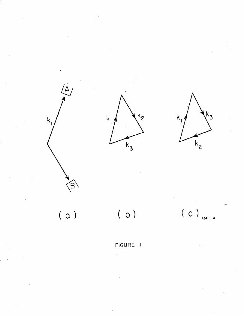
To show this, consider an event where

one of three photonsgoes into A and another into 53. The probability of this

event (see Fig. lla) is independent of whether there is a detector at B or

not. Now corresponding to this event, there are two possibilities, either

k goes into B or k goes into B as shown in Fig. lib and 11~. Both of 2 3

these possibilities occur when there is no detector at B. But now as soon

- 28 -

I

as we put a detector in B, the situation represented by Fig. llc is excluded

because we said the photon detected by B is called k2 . This proves our

assertion. The result can be generalized to n identical particles in the

final states. We need n-l detectors to determine the kinematics of the

problem. Thus if there are n-l detectors we use the standard rule. If we

have n-2 detectors we divide the whole expression by 2. If there are n-d

detectors we divide the standard expression by d! Specifically if there is

no detector (i.e. total cross section) we have to divide the Eq. (A-l) by n!

The arguments given above can be used in our calculation of spectra of

k + dueto e +e--+3y. The radiative corrections calculated by Brown and 1

Feynman and Harris and Brown apply only to the coincidence experiments. Since

we are not measuring k and k 2 3

we have to integrate over all the phase

space of k and k and divide it by 21 according to our prescription. The 2 3

phase space of k and k 2 3

can be represented as an ellipsoid as shown in

Fig. 9. Now the matrix element M * I 1 is symmetric with respect to interchange

of k2 *k . 3

Thus instead of integrating k2 and k3 in the whole phase

space and divide it by 2! , we may equivalently integrate half of the phase

space as shown in Fig.10 . Now in this modified phase space k2 is never

small and thus infrared divergence occurs only when k -+o,, although both 3

k and k 2 3

can become infrared in the complete phase space.

-29 -

REFERENCES AND FOOTNOTES

1. J. Ballam and Z.G.T. Guiragossian, "Almost monochromatic photon beams

at the Stanford Linear Accelerator Center." Proceedings of the Inter-

national Conference on High-Energy Physics, Dubna, 1964.

2. Swanson, Iddings and Tsai, to be published.

3. ox, ay and 0s are usual 2 X 2 Pauli matrices.

4. There is an error in Eq. (12-48) of Jauch and Rohlich: "Theory of photons

and electrons." First Edition. In the Second Edition the correct formula

was given.

5. I. Harris and L. M. Brown, Phys. Rev. 105, 1656 (1957). Hereafter referred

to as H. B.

6. L. M. Brown and R. P. Feyrman, Phys. Rev. 3, 231 (1951). Hereafter re-

ferred to as B. F.

7. We give this expression in detail because there are two misprints in Eq. 3,

and wrong sign for Eq. (Sa) of H. B. The present author did not check.their

calculation in complete detail. The errors were found by comparing with the

results of 13. F. According to Professor Brown, the results in B. F. are more

correct.

2. This expression is very similar to Eq. 43 of B. F. except for the terms pro-

portional to f12 in f.

9. Y. S. Tsai, Phys. Rev. 122, 1893 (1961).

10. The advantage of using the center of mass system is that it is easier to see

under what conditions the k in the numerator of the matrix element can be 3

neglected and obtain an extremely simple expression such as Eq. (3-16). From

our considerations it can be concluded that in order to neglect k in the 3

-30 -

numerator, it is not necessary to assume Lu to be much smaller than m 3

in the laboratory system as was done in B. F. and H. B. As will be argued

in Section 5, in the regions where cu << m in the lab system, the pertur- 3

bation expansion is not valid due to the existence of terms like pn22y

in the radiative corrections 6. Similar consideration was done by the

author for the radiative correction to the e-e scattering in the labor-

atory system. See Section 5 of the paper Y. S. Tsai, Phys. Rev E, 269

(MO).

11. See footnote 17.

12. The approximations made here are certainly the most serious ones and impose

severe limitations to the range of applicability of our result, represented

by the first inequality in (3-30) and inequalities (3-31). The problem that

one has to investigate is whether the curve in Fig. 7 goes down monotonically

to the low energy end or will it go up again and give some additional (unwelcome)

low energy photons. The author tends to believe the latter because a positron

can first emit a high energy photon and then annihilate at a very low energy

at which the cross section is very large. (A similar phenomenon is well

known in the bremsstrahlung produced by coulomb scatterings.) Fortunately-

the exact calculation of low energy end of the spectrum can be done without

much difficulty with the help of a computer. A computer can take traces,

sum the tensor indices, do necessary cancellations, sorting out terms in a

convenient order and obtain an analytical expression in less than one hour

for a job which takes about six months for a physicist to do by paper and

pencil. Two working computer procedures are available at Stanford, one by

- 31 -

S. Swanson and another by A. Hearn, both of the Physics Department,

Stanford University.

13. Inequalities (3-17) reduce to (3-31) in the laboratory system. Fortunately

the angular range most convenient for the experimentalists' is in the

vicinity.of ye’/2 N + to 4 and thus these inequalities are easily

satisfied.

14. See the discussion concerning Eq. (l-4) of Ref. 9.

15. See D. R. Yennie, S. C. Frantschi, H. Suura: Annals of Physics 0; 3i9 (196l),

Appendix C.

16. See Section 4 for numerical examples, (- a/fl f = Y).

17. If we believe in Schwinger's conjecture that the radiative corrections to all

order can probably be written as e 6 cl2 = i + 6 + __- + . . . . . then for 2! - b < 0.2, -

the next order correction will be expected to be less than 2%.

18. Brown and Feynman's results (Ref. 6) show that after renormalization and

infrared cancellation, only the matrix element represented by J in Fig. 5

contains logarithmic terms when inequalities (3-3a,b) are satisfied. Thus

our observation can be stated simply that the bulk of the contribution

from the matrix element J to the radiative corrections can be obtained from

the Schwinger vertex correction by a substition -t 4s.

-2 -

LIST OF FIGURES

1. A typical gamma spectrum of positron hydrogen atom collision at a fixe'd

angle.

2. Lowest order Fey-nman diagrams for the interaction ec f e- +27.

3. Coordinate system used in the discuss‘ion of polarization of photons.

k2 is chosen to be on the x-z plane.

4. Polarization vectors used in the definition of Stokes parameters for the

photon ki.

5. Feynman diagrams for virtual radiative corrections.

6. Feynman diagrams for real radiative corrections.

7. A typical energy spectrum of the photon at a fixed angle. The point

UF(eave) is chosen to be the value of u) 1 determined by two body

final state kinematics at the average angle of the detector. &i

should be chosen such that w << hOi << w et 0 1 . . 1

8. The phase space for k in the center of mass system is represented 1

by the area ABCD. We approximate ABCD by ABC'D' .

9. An ellipsoid representing the phase space for k2 and k in the center 3

of mass system. ii connects the two foci of the ellipsoid. The 1

ellipsoid has a maximum extension when G -m

=cu . 1 1

10. The semiellipsoid to be used to determine omax as a function of 3

e13 ( angle between 'Y1 and k3).

11. Three identical particles in the final state. (a) One particle k1 goes

into detector A and another goes into direction B. (b) k goes into B. 2

(c) k3 goes into B.

Te'+e--2y

-+Y

f

e++p--e+tpty

134-I-A

FIGURE I

k I k 2

4

P 2

k 2 k I 4

P I P 2

134-2-A

FIGURE 2

X 134-3-A

FIGURE 3

A A -

e,+ie Y

ex+ ey A

lff * / e,- i$

fl t--k’ 7E

134-4 -A

FIGURE 4

I

L N’ N” 134-5-A

FIGURE 5

M I M 2 M 3

M 4 M 5 M 6 134.6.A

FIGURE 6

min al WI

e’ c

134-7-A

FIGURE 7

I A - WI

i C’ _---- -- ----

8 min 9 WI

8 max 134-8-A

FIGURE 8

1 -

\ I

P 2

I34- 9-A

FIGURE 9

-

E

1

k I

----- ---- l- -- _--- -- l-

134-10-A

FIGURE IO

(0) (b)

FIGURE II

Cc) 134-11-A