I --_

SLAC-PUB-5702 LBL-30724 November 199 1 W

Alternative Positron-Target Design for Electron-Positron Colliders*

Richard J. Donahue ‘F Environment, Health and Safety Division’:

Lawrence Berkeley Laboratory University of California

Berkeley, California

W. R. Nelson Environment,Safety and Health Division $

Stanford Linear Accelerator Center Stanford University

Stanford, California 94309

ABSTRACT

Current electron-positron linear colliders are limited in luminosity by the number of positrons which can be generated from targets presently used. This paper examines the possibility of using an alternate wire-target geometry for the production of positrons via an electron-induced electromagnetic cascade shower.

.-- --- .-- .

*Work supported by the Department of Energy, contract DE-AC03-76SFOO515 t Partial fulfillment for M. S. Degree at University of Lowell $ Work supported by the Department of Energy, contract DE-AC03-76SF00098

1. Introduction

One of the major design problems which must be overcome for the next gen-

eration of electron-positron colliders is a source of positrons which will meet the

projected luminosity (cmm2) requirements”]. These luminosity requirements are

‘at--least a factor of one hundred higher than for present-day e+e- colliders. One

method to increase luminosity is to reduce the cross-sectional area (a, x cry) of the

colliding beams. The other way is to increase the beam current. The e+ target

currently used at the Stanford Linear Collider (SLC) is approaching its design lim-

itation, so there is considerable incentive to find new ways to produce the needed

number of positrons I”. This paper explores the idea of using a thin cylinder, or

wire, to produce positrons as an alternative to the semi-infinitegeometry now used.

2. Properties of the Electromagnetic Cascade Shower

2.1 GENERAL

When charged particles are transported through a material, they lose energy

through collisions and radiation processes. Collision processes result from excita-

tion and/or ionization of atoms in the material. Energy is lost through secondary

electron emission and is deposited locally. This process accounts for the majority of

- the heat deposition in targets. Energy loss by radiation processes (i.e., bremsstrah-

lung) is distributed among secondary particles whose energy may reach the energy

of the incident electron. At high incident electron energies this is the dominant

energy-loss mechanism. The dominant photon cross section at high energies is pair

production, or materialization, whereby an electron-positron pair is created. The

electron-positron pairs can also radiate bremsstrahlung photons. This sequence

continues, with the energy of each newly created particle decreasing with each

interaction, resulting in what is called an electromagnetic (EM) cascade shower.

2

t= 0

h’=‘t= 1

E/&) = 2-t = 1

e- -

1 2 3 4 r.1. 2 4 S __ 16

l/2 l/4 l/S l/16

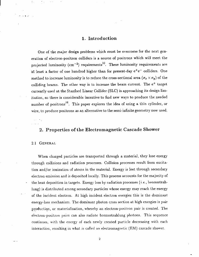
Fig. 1. Simplified schematic of the initial portion of an EM cascade shower

Figure 1 is a simplified schematic of the initial portion of a high-energy shower.

The horizontal axis has units of radiation lengths, along side of which the number

of secondaries (e*, y), as well as the energy of each secondary, is indicated. From

this diagram one can deducet’lthat the number of secondaries is proportional to the

incident energy, Es, and inversely proportional to the cutoff energy, E,,t. Namely,

(3.1)

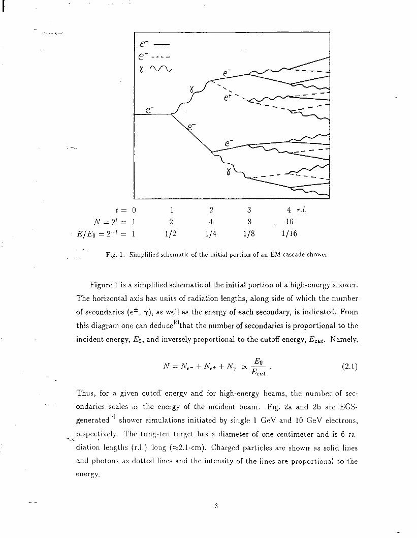
Thus, for a given cutoff energy and for high-energy beams, the number of sec-

ondaries scales as the energy of the incident beam. Fig. 2a and 2b are EGS-

generated”] sho\ver simulations initiated by single 1 GeV and 10 GeV electrons,

-=-. .-- -respectively. The tungsten target has a diameter of one centimeter and is 6 ra-

diatio; lengths (r.1.) I ong (z2.1-cm). Charged particles are shown as solid lines

and photons as dotted lines and the intensity of the lines are proportional to the

energy.

3

: .‘. : : :’ . . .: .. .A::. : : J: : .. :’ /

Fig.-,i: i3GS4 (graphical) simulation”’ of an EM cascade shower: a) 1 GeV, b) 10 GeV.

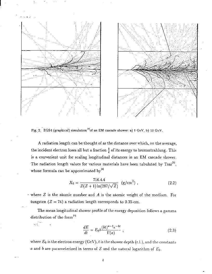
A radiation length can be thought of as the distance over which, on the average,

the incident electron loses all but a fraction i of its energy to bremsstrahlung. This

is a convenient unit for scaling longitudinal distances in an EM cascade shower.

The radiation length values for various materials have been tabulated by Tsai[‘],

whose formula can be approximated by@]

x0 = 716.4A

Z(Z + 1) ln(287/fi) Wcm2) 7 P-2)

- where 2 is the atomic number and A is the atomic weight of the medium. For

tungsten (2 = 74) a radiation length corresponds to 0.35-cm.

The mean longitudinal shower profile of the energy deposition follows a. gamma

distribution of the form”’ .-- =- .- .

dE,Eb dt

o (bty-‘e-bl

w> ’ (2.3)

where Es is the electron energy (GeV), t is the shower depth (r.l.), and the constants

a and b are parameterized in terms of 2 and the natural logarithm of Ea.

4

I

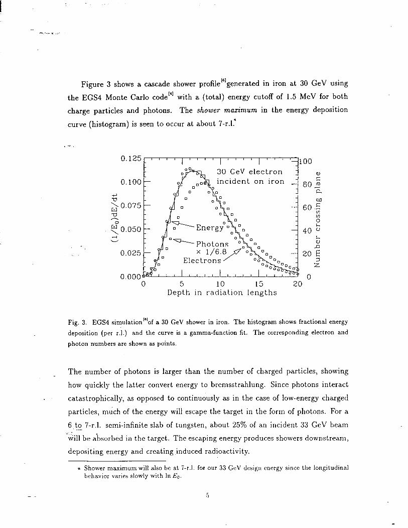
Figure 3 shows a cascade shower profile”‘generated in iron at 30 GeV using

the EGS4 Monte Carlo code”’ with a (total) energy cutoff of 1.5 MeV for both

charge particles and photons. The shower maximum in the energy deposition

curve (histogram) is seen to occur at about 7-r.l.*

30 GeV electron incident on iron

0 5 10 15 20 Depth in radiation lengths

Fig. 3. EGS4 simulation’6’ of a 30 GeV shower in iron. The histogram shows fractional energy

deposition (per r.1.) and the curve is a gamma-function fit. The corresponding electron and

photon numbers are shown as points.

The number of photons is larger than the number of charged particles, showing

how quickly the latter convert energy to bremsstrahlung. Since photons interact

catastrophically, as opposed to continuously as in the case of low-energy charged

particles, much of the energy will escape the target in the form of photons. For a

S-to 7-r.1. semi-infinite slab of tungsten, about 25% of an incident 33 GeV beam

~111 be absorbed in the target. The escaping energy produces showers downstream,

depositing energy and creating ,induced radioactivity.

* Shower maximum will also be at 7-r.1. for our 33 GeV design energy since the longitudinal behavior varies slowly with In Ee.

The current SLC target is about one centimeter in diameter and 6-r.1. long.

It was designed”’ slightly less than 7-r.l., since a disproportionately large fraction

of the energy is absorbed near shower maximum-i.e., making the target a little

shorter reduces the total power absorbed in the target, which in turn decreases

both radioactivity and temperature-rise problems. I -_.

After briefly discussing the general characteristics of the EM cascade shower,

the fundamental interactions which produce the cascade are discussed. These are

pair production for photons and bremsstrahlung for charged particles.

2.2 PHOTON INTERACTIONS

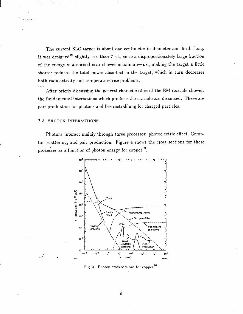
Photons. interact mainly through three processes: photoelectric effect, Comp-

ton scattering, and pair production. Figure 4 shows the cross sections for these

processes as a function of photon energy for copper[gl.

..- =_ Tw

Paatikluq (Kern)

10.2 10.' 100 10’ 102 10’ 10’ 10’ Ue k (Me’4 rrrYl

Fig. 4. Photon cross sections for c~pper’~‘.

I :

Note that above about 10 MeV, the photonuclear cross sections (giant resonance,

quasi-deuteron, pion production) come into play, but these cross sections are down

by 13 to 3 orders of magnitude.

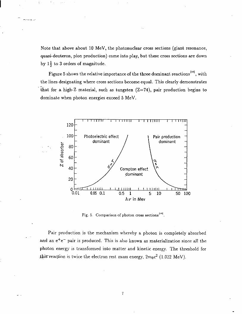
Figure 5 shows the relative importance of the three dominant reactions “‘l, with

the lines designating where cross sections become equal. This clearly demonstrates L --

that for a high-Z material, such as tungsten (Z=74), pair production begins to

dominate when photon energies exceed 5 MeV.

I I I Illlll I I I111111 I I I111111 I IIInTrr

120 -

100 - Photoelectric effect Pair production - dominant dominant

80-

60

40

0.05 0.1 0.5 1 5 10 50 100 hv in Mev

Fig. 5. Comparison of photon cross sections’lol.

Pair production is the mechanism whereby a photon is completely absorbed

and an e+e- pair is produced. This is also known as materialization since all the

photon energy is transformed into matter and kinetic energy. The threshold for

&hisreac.tion is twice the electron rest mass energy, 2moc2 (1.022 MeV).

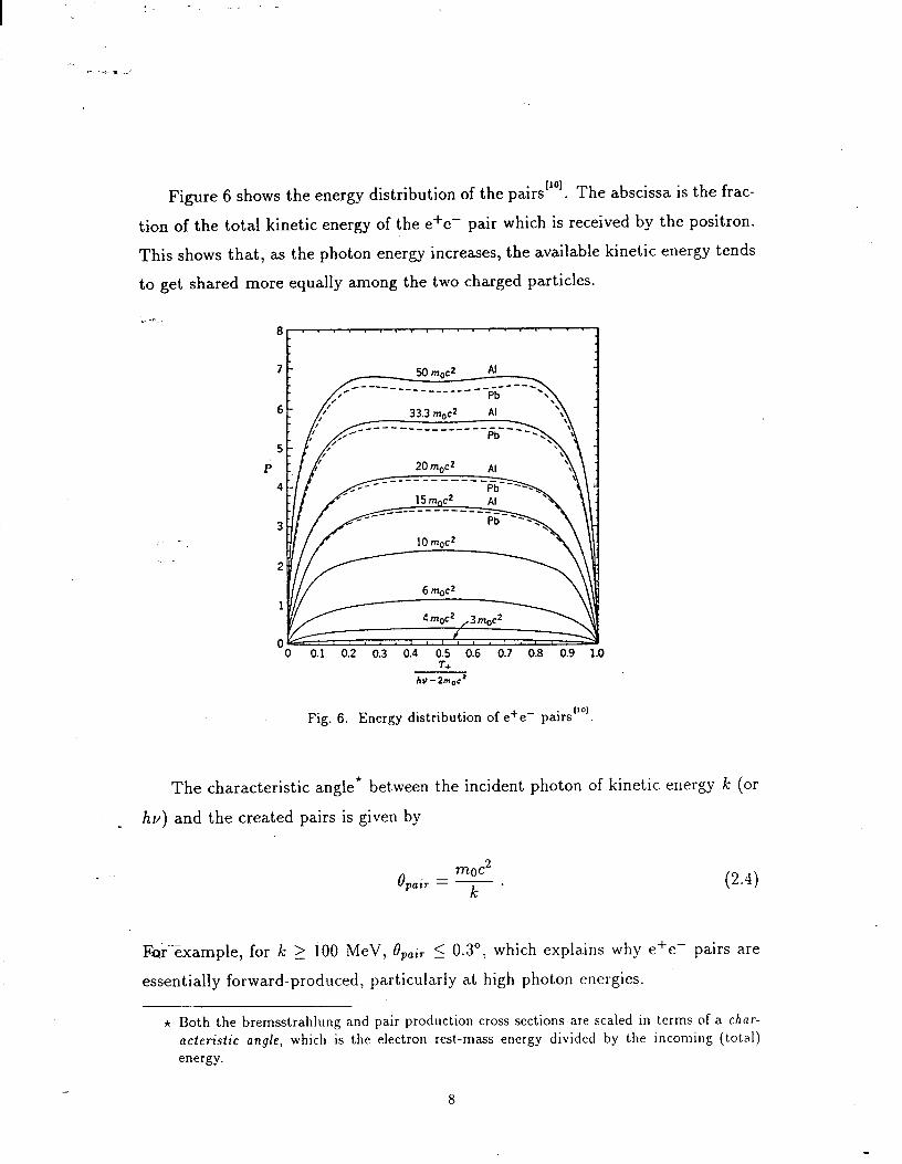
Figure 6 shows the energy distribution of the pairs”‘]. The abscissa is the frac-

tion of the total kinetic energy of the e+e- pair which is received by the positron.

This shows that, as the photon energy increases, the available kinetic energy tends

to get shared more equally among the two charged particles.

7 7

6 6

5 5 i i

4 4

3 3

2 2

1 1

0 0 0 0 0.1 0.2 0.3 0.4 0.5 0.6 0.7 0.8 0.9 1.0 0.1 0.2 0.3 0.4 0.5 0.6 0.7 0.8 0.9 1.0

hv-2m.c’

Fig. 6. Energy distribution of e+e- pairs”‘].

The characteristic angle* between the incident photon of kinetic energy k (or

hv) and the created pairs is given by

For%xample, for k > 100 MeV, epair _ < 0.3”, which explains why e+e- pairs are

essentially forward-produced, particularly at high photon energies.

* Both the bremsstrahlung and pair production cross sections are scaled in terms of a char- acteristic angle, which is the electron rest-mass energy divided by the incoming (total) energy.

8

I :

The attenuation coefficient (i.e., cross section) for pair production varies as

KE Z*lnk (2.5)

for low values of k, and as ; --_ 7

K21Z2- 9x0

P-6)

for high energies, where X0 is the radiation length of the material. Pair production

is induced by the strong electric field surrounding the nucleus. At large distances

from the nucleus the electric field is screened by the orbital electrons, and this

screening becomes important for high-Z materials and high energies.

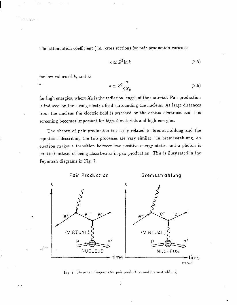
The theory of pair production is closely related to bremsstrahlung and the

equations describing the two processes are very similar. In bremsstrahlung, an

electron makes a transition between two positive energy states and a photon is

emitted instead of being absorbed as in pair production. This is illustrated in the

Feynman diagrams in Fig. 7.

X

Pair Production Bremsstrahlung

X I

NUCLEUS - time

NUCLEUS ‘- time

1?6?*rJ

Fig. 7. Feynman diagrams for pair production and bremsstrahlung

9

If you reverse the e+ arrowhead in the pair production diagram, and change

it to an e- traveling forward in time, then the diagram is identical to the brems-

strahlung diagram. In other words, the two processes are alike.

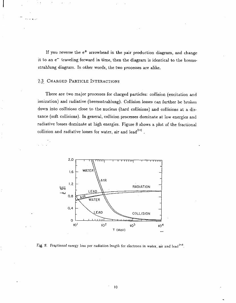
2.3. CHARGED PARTICLE INTERACTIONS

There are two major processes for charged particles: collision (excitation and

ionization) and radiative (bremsstrahlung). Collision losses can further be broken

down into collisions close to the nucleus (hard collisions) and collisions at a dis-

tance (soft collisions). In general, collision processes dominate at low energies and

radiative losses dominate at high energies. Figure 8 shows a plot of the fractional

collision and radiative losses for water, air and lead”” .

1.6

IO3 IO4 T (MeV) I-

Fig; 2~ Frclctional energy loss per radiation length for electrons in water, air and lead”“.

10

The crossover point where radiative and collision losses are equal is called the

critical energy and can be approximated by’12’

e N z”,“ye2 (MeV) . (2.7)

The critical energy is about 10 MeV for lead and 100 MeV for water, which points

to the energy at which EM showers become significant in those materials. The ratio

between radiative and collision losses (i.e., stopping powers) can be approximated

T > 1600moc2 ’ (2.8)

which shows that radiative losses increase linearly both with 2 and the electron

kinetic energy. Therefore, for a beam of 33 GeV electrons, bremsstrahlung is the - most important interaction. It should be noted, however, that as the energies of the

secondary electrons fall below the critical energy (11 MeV for tungsten), collision

losses will begin to dominate.

Continuing with the bremsstrahlung process, whenever a charged particle trav-

eling through matter is deflected from its path, or has its velocity changed, it may

emit electromagnetic radiation whose energy is proportional to the deceleration re-

ceived by the charged particle. This deceleration is caused by the influence of the

electric field of the target nucleus on the particle. The radiation emitted is called

bremsstrahlung (breaking radiation) and the high-energy (i.e., complete screening)

cross section is expressed asL31

11

where

I -_.

E = incident electron energy (GeV),

E’ = scattered electron energy (GeV),

k = photon energy = E - E’ (GeV),

2 = atomic number,

A = atomic mass (g mol-‘),

cy = fine structure constant = l/137 ,

iVo = Avogadro’s number = 6.02 x 1O23 (mol-‘) ,

ro = classical electron radius = 2.82 x lo-l3 (cm) .

Two important observations can be made from this equation:

l -The cross section is proportional to Z2- i.e., high-2 materials are more

likely to radiate than low-2 materials.

l The spectrum has a l/k shape--i-e., low-energy photons are more probable

than high-energy ones.

At relativistic energies the scattered electron and the emitted photon tend to

proceed in the same direction as the incident electron (i.e., the distribution is

highly forward-peaked). As in the case of pair production described above, the

differential cross section for bremsstrahlung is scaled in terms of a characteristic

angle given by””

8 ?7-10C2

brem = - E ’ (2.10)

where E is the (total) energy of the incident electron. Kate again that ebrem 5 0.3’

for E 2 100 MeV. ..-

-” Althotigh the longitudinal development of the shower is dominated primarily by

bremsstrahlung and pair production interactions, the lateral spread of the cascade

is governed by elastic Coulomb scatterin, c of the charged-particle component. The

individual deflections are a.dequately described by the Mott formula 1131 which, as

12

in the case of Rutherford scattering, has a 6-4 dependence. What this implies

is that most of the scattering interactions lead to very small deflections. Small

& deflections are generally the result of a large number of very small deflections;

whereas, large net deflections are the result of a single large-angle scatter plus a

number of very small deflections. The overall picture of charged-particle scattering

is--a medium can be viewed as a Gaussian-like distribution controlled by small-

angle scattering, referred to as multiple scattering, superimposed onto which is a

single-scattering (large-angle) tail* .

Multiple scattering is best described analytically by the Fermi-Eyges model

(e.g., see Chapter 3 of Kase and NelsonL”‘), the form of which is a Gaussian

measured in terms of a root mean square projected angle given by

- e sms N y (radians) , (2.11)

where t is the material thickness in radiation lengths and E is the charged-particle

energy in MeV. If we now equate the characteristic angle of bremsstrahlung (Obrem)

to the rms scattering angle (O,,,) and solve for the thickness, we get

t= mot

2 2 [ I - M 0.001 r.1. 15

(2.12)

In other words, charged particles scatter significantly prior to losing much energy by

radiative interactions. In effect, this is a clear demonstration of the statement made

earlier regarding the lateral spread of EM cascades being controlled by charged-

particle scattering.

* The region joining the two distributions in a smooth manner is oken referred to as the plural scafiering region’ll’.

13

3. The EGS4 System

3.1 GENERAL

The EGS4 (Electron-Gamma-Shower version fl) Code System is a collection of

programs for the Monte Carlo simulation of coupled electron-photon transport”‘.

It is designed to be used in any geometry and for energies from a few keV up to

several TeV. The system was first introduced1141 in 1978 and was simply referred

to as EGSS. Because of its versatility and relative ease-of-use, and because it has

been checked against many experiments, EGS4 has been used rather extensively by

the particle physics community in the development of shower counters and related

detectors. There has also been a growing use of EGS4 by the medical physics

community for modeling the transport of electrons and photons down to a few keV

in complex geometries, including the human body. -

3.2 CAPABILITIES AND FEATURES OF THE CODE

The following summarizes the main features of the EGS4 Code System:

l EGS4 is a package of subroutines plus block data with a flexible user interface.

l Electrons (zt) and photons can be transported in any element, compound, or

mizture.

l The dynamic range of electron (IL) kinetic energies goes from a fe\v tens of

keV up to a few thousand GeV.

l The dynamic range of photon energies lies between 1 keV and several thou-

sand GeV.

l A data preparation code (PEG!%) creates data from cross-section tables for ..-

- elements 1 through 100. The output is in a form for subsequent direct use

by EGS4.

l The geometry for any given problem is specified by a user-written subroutine

called HOM’FAR.

14

l The user scores and outputs information in the user-written subroutine called

AUSGAB.

l The EGS4 Code System is written in an extended FORTRAN language

known as Mortran3[151.

; -.. l Variance reduction techniques are not built into EGS4 per se, but can be

implemented by means of a macro facility available through Mortran3.

l Transport can be initiated from sources having spatial, angular, or energy

distributions.

3.3 PHYSICS PROCESSES IN THE EGS4 CODE SYSTEM

The following physics processes are taken into account by the system:

- i Electron (5) bremsstrahlung.

l Positron annihilation at rest and in flight (annihilation quanta followed to

completion).

l Multiple Coulomb scattering of electrons (III) from nuclei (Moliere model).

l Delta-ray production by means of e-e- (Moller) and e+e- (Bhabha) scat-

tering.

l Continuous energy loss applied to electron (f) tracks between discrete in-

teraction sites using a restricted stopping power (i.e., Bethe-Bloch formula

including Sternheimer density effect correction).

l Pair production.

0 Compton scattering.

7. : ..-a Coherent (Rayleigh) scattering .

l Photoelectric effect (including Ii-edge fluorescent photon production).

15

3.4 STRUCTURE AND OPERATION

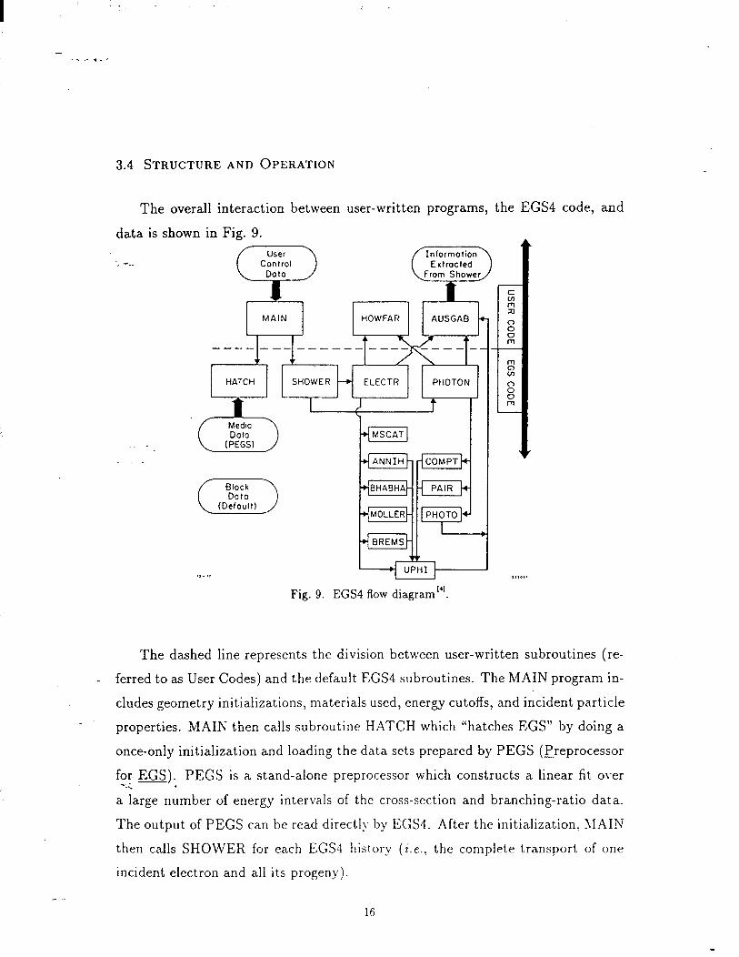
The overall interaction between user-written programs, the EGS4 code, and

data is shown in Fig. 9. / User \ L -.. Control

Doto

w

IMCilN/

finformotion\

iOWER PI

ELECTR I I PHoToN I I

Fig. 9. EGS4 flow diagram”‘.

The dashed line represents the division between user-written subroutines (re-

ferred to as User Codes) and the default EGS4 subroutines. The MAIN program in-

cludes geometry initializations, materials used, energy cutoffs, and incident particle

properties. MAIN then calls subroutine HATCH which “hatches EGS” by doing a

once-only initialization and loadin g the data sets prepared by PEGS (Preprocessor

for- ms). PEGS is a stand-alone preprocessor which constructs a linear fit over -. : . a large number of energy intervals of the cross-section and branching-ratio data.

The output of PEGS can be read directI\- by EGS4. After the initialization, \lAIN

then calls SHOWER for each EGS-1 history (i.e., the complete transport of one

incident electron and all its progeny).

16

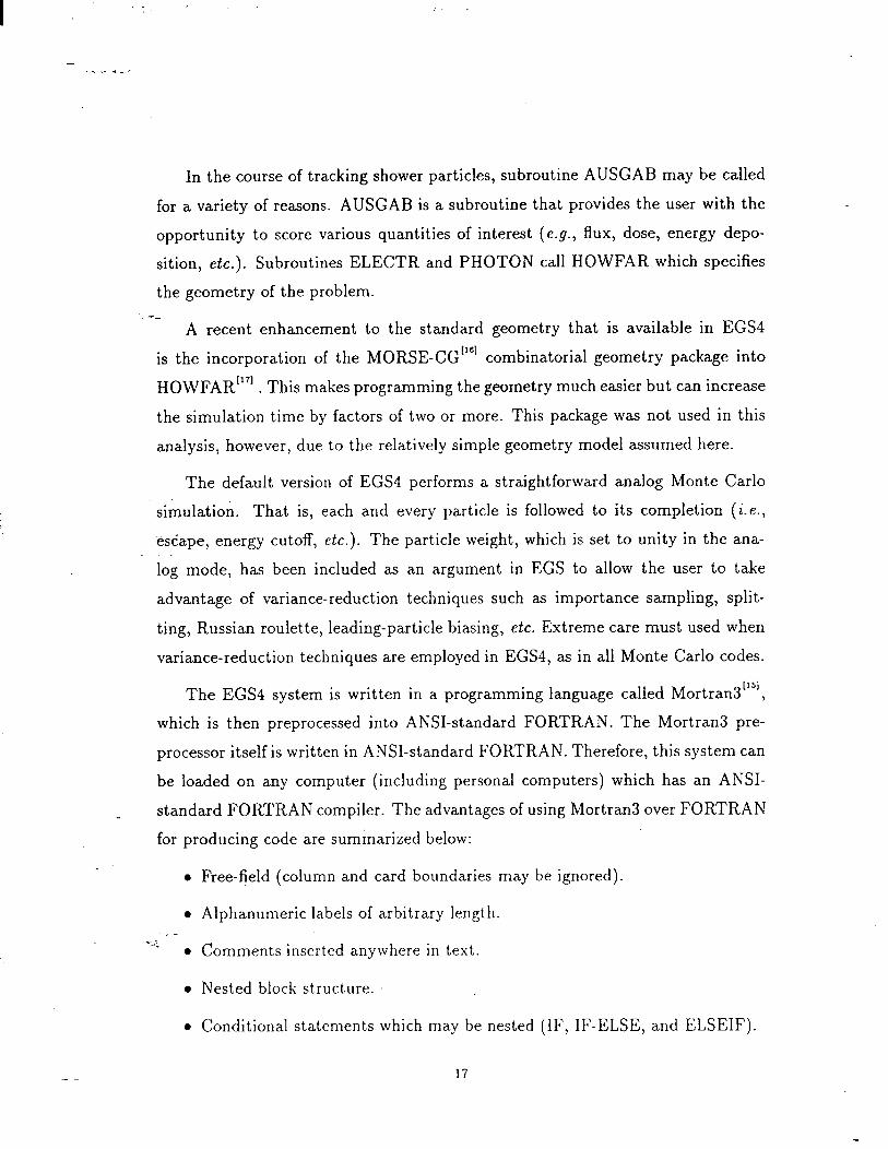
In the course of tracking shower particles, subroutine AUSGAB may be called

for a variety of reasons. AUSGAB is a subroutine that provides the user with the

opportunity to score various quantities of interest (e.g., flux, dose, energy depo-

sition, etc.). Subroutines ELECTR and PHOTON call HOWFAR which specifies

the geometry of the problem. I --_

A recent enhancement to the standard geometry that is available in EGS4

is the incorporation of the MORSE-CG”“’ combinatorial geometry package into

HOWFAR”” . This makes programming the geometry much easier but can increase

the simulation time by factors of two or more. This package was not used in this

analysis, however, due to the relatively simple geometry model assumed here.

The default version of EGS4 performs a straightforward analog Monte Carlo

simulation. That is, each and every particle is followed to its completion (i.e.,

escape, energy cutoff, etc.). The particle weight, which is set to unity in the ana- - log mode, has been included as an argument in EGS to allow the user to take

advantage of variance-reduction techniques such as importance sampling, split-

ting, Russian roulette, leading-particle biasing, etc. Extreme care must used when

variance-reduction techniques are employed in EGS4, as in all Monte Carlo codes.

The EGS4 system is written in a programming language called Mortran3”“,

which is then preprocessed into ANSI-standard FORTRAN. The Mortran3 pre-

processor itself is written in ANSI-standard FORTRAN. Therefore, this system can

be loaded on any computer (including personal computers) which has an ANSI-

standard FORTRAN compiler. The advantages of using Mortran3 over FORTRAN

for producing code are summarized below:

l Free-field (column and card boundaries may be ignored).

l Alphanumeric labels of arbitrary length. ..-

l Comments inserted anywhere in text.

l Nested block structure.

l Conditional statements which may be nested (IF, IF-ELSE, and ELSEIF).

17

l Loops (repetitively executed blocks of statements) which test for termination

at the beginning or end or both or neither (WHILE, UNTIL, FOR-BY-TO,

LOOP, and DO).

l EXIT (jump out of) any loop. Multiple assignment statements. Conditional

I -- (multiple) compilation. Program listing features include:

- Automatic printing of the nesting level.

- Automatic indentation (optional) according to nesting level.

l Abbreviations for simple I/O statements.

l Interspersion of FORTRAN text with Mortran text.

In addition, however, Mortran3 has an extensive macro-facility such that many

FORTRAN steps can be accomplished in just a few Mortran steps. Users can .- also write their own macro’s that redefine the default language. This makes the

language “open- ended”--i. e., the user can make extensions to the language at any

time to suit the problem.

The Mortran3 language is an example of why EGS4 is relatively easy to use;

the coding is easier to read than FORTRAN. This greatly simplifies writing new

code and especially in modifying previously written code.

3.5 GRAPHICS CAPABILITIES

EGS4 has been coupled with the SLAC Unified Graphics System’18’ for dis-

playing particle tracks on UGS77-supported devices”gl. It has also been modified

to display the distribution of induced radioactivity in beam targets’201.

-i This is accomplished by inserting the SHOWGRAF package onto the User Code

and then making the CALL statements in the appropriate places in AUSGAB. The

graphical output may be displayed directly onto an IBM 5080 color terminal which

supports three-dimensional rotations, translations, and zooming. SHOWGRAF

18

can also output graphics into files for printing on a PC display using a post-

processor system called EGS4PL”“. Figure 10 is an example of an output from

SHOWGRAF.

” -_.

Fig. 10. EGS4 simulation of 8.5 MeV electrons scattering in a 0.38-mm copper foil (100 events). A 2.6 kG magnetic field focuses the electrons through a lead slit. Solid lines are

electrons and dots are photons.

3.6 BENCHMARKS

As stated earlier, EGS4 is used extensively throughout the world in both the

high-energy physics and the medical physics communities. Perhaps the most im-

pressive benchmarks are performed by the users and the results of these benchmarks

,,can be.demonstrated by the growing number of EGS4 users. A recent book entitled

Monte Carlo Transport of Electrons and I’hoto~‘~‘~ provides a good collection of

these benchmarks that have been performed by various authors.

19

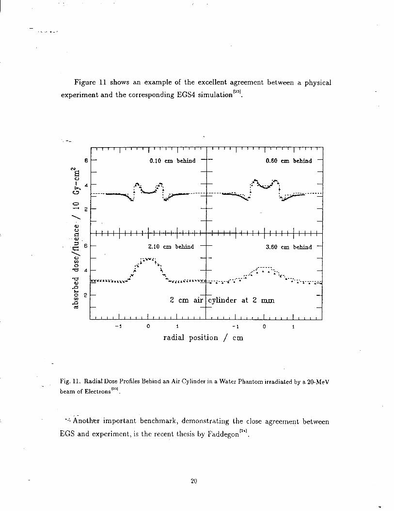
Figure 11 shows an example of the excellent agreement between a physical

experiment and the corresponding EGS4 simulation I231 .

Fig. 11. Radial Dose Profiles Behind an Air Cylinder in a Water Phantom irradiated by a 20-MeV

beam of Electrons’33’.

-i Another important benchmark, demonstrating the close agreement between

EGS and experiment, is the recent thesis by Faddegon”“.

20

4. ETRANS

ETRANS l is a Pascal/FORTRAN/Mortran program that follows electrons (zt),

one at a time, through an electromagnetic field having rotational symmetry about

the incident electron beam direction. The program was written at SLAC P51 to

‘model the transport of positrons in the capture section (i.e., e+ collector) down-

stream of the SLC positron target. The capture section consists of the following:

1. A set of magnetic solenoids.

2. A flux concentrator which provides a very high, rapidly varying field.

3. Accelerator sections.

The experimental results agree quite well with predictions by ETRANS, using

EGS-generated e+ input, for the current SLC target scheme.

5. SLC Positron Target

The SLAC Linear Collider (SLC) is an electron-positron machine system de-

signed to accelerate and collide two 50 GeV beams (see Fig. 12). Electrons are

emitted from a thermionic gun and accelerated to 1 GeV. A splitter magnet deflects

electrons and positrons into separate damping rings where synchrotron radiation

reduces their transverse emittance. One positron bunch’ and two electron bunches

are ejected and accelerated down the linac. The positron bunch and the first of the

electron bunches are accelerated to about 50 GeV. The two bunches are separated

and transported around the arcs, bringing them into collision at the interaction

point. The bunches are then deflected into beam dumps. The second electron

bunch is extracted at the 2/3 point in the linac, where its energy is 33 GeV, in .--

‘brder to produce positrons. Positrons are then captured, accelerated, and returned

to the front end of the linac for further acceleration into the damping ring.

* Not to be confused with the ETRAN Monte Carlo program l-4 t A bunch is typically 1 to 2 x 10” e+ or e-.

21

POSITRON SOURCE Constant Groditnt

Acctltrotor

Positron Domping Pulsed Soknoid

Torqtt 8 DC !+knoid Extraction Lint

I / - b/

- 200 t&V/c t* Return Lane

,‘ Electron Dompinp .-., Ring fnol lo scolel

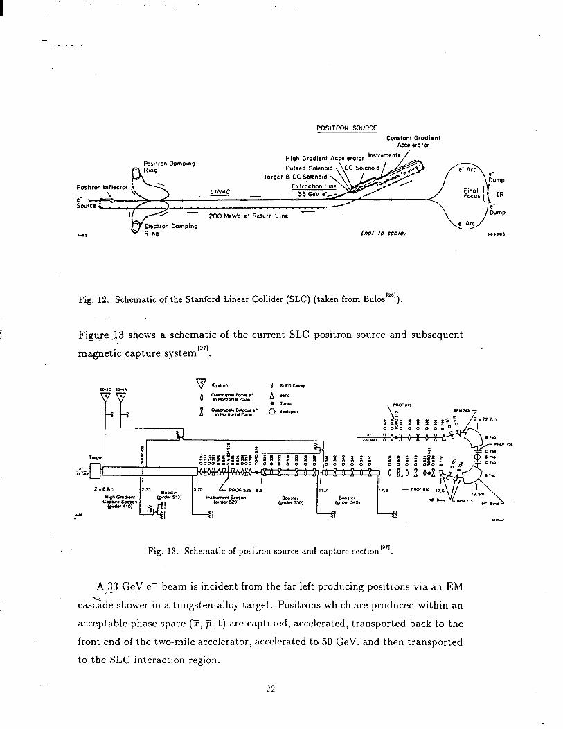
Fig. 12. Schematic of the Stanford Linear Collider (SLC) (taken from BI.IIos’~~~)

Figure.13 shows a schematic of the current SLC positron source and subsequent 1271 magnetic capture system .

Fig. 13. Schematic of positron source and capture section”‘l.

4 33 GeV e- beam is incident from the far left producing positrons via an EM ..- cascade shower in a tungsten-alloy target. Positrons which are produced within an

-- acceptable phase space (x, p, t) are captured, accelerated, transported back to the

front end of the two-mile accelerator, accelerated to 50 GeV, and then transported

to the SLC interaction region.

2‘2

.

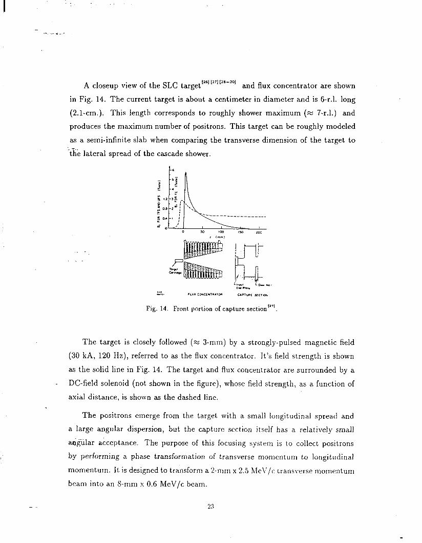
A closeup view of the SLC target1261’271’28-301 and flux concentrator are shown

in Fig. 14. The current target is about a centimeter in diameter and is 6-r-l. long

(2.1-cm.). This length corresponds to roughly shower maximum (Z 7-r.1.) and

produces the maximum number of positrons. This target can be roughly modeled

as a semi-infinite slab when comparing the transverse dimension of the target to ; --. the lateral spread of the cascade shower.

Fig. 14. Front portion of capture section”“.

The target is closely followed (z 3-mm) by a strongly-pulsed magnetic field

(30 kA, 120 Hz), f re erred to as the flux concentrator. It’s field strength is shown

as the solid line in Fig. 14. The target and flux concentrator are surrounded by a

- DC-field solenoid (not shown in the figure), whose field strength, as a function of

axial distance, is shown as the dashed line.

The positrons emerge from the target with a small longitudinal spread and

a large angular dispersion, but the capture section itself has a relatively small

ar$ilar acceptance. The purpose of this focusing system is to collect positrons

by performing a phase transformation of transverse momentum to longitudinal

momentum. It is designed to transform a 2-mm x 2.5 MeV/c transverse momentum

beam into an S-mm x 0.6 MeV/c beam.

23

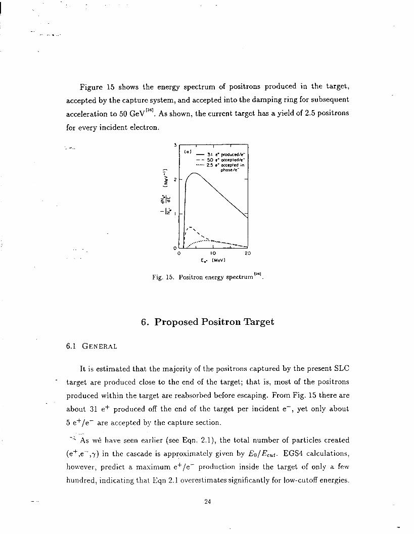
Figure 15 shows the energy spectrum of positrons produced in the target,

accepted by the capture system, and accepted into the damping ring for subsequent

acceleration to 50 GeV’261. As shown, the current target has a yield of 2.5 positrons

for every incident electron.

” -._

i

2

I

0

I I 8 (0) - 31 l * produced/e-

- - 50 l * oacPted~e- *-*** 2.5 e’ occepled in

phoscle-

0 IO E.- (MeV)

Fig. 15. Positron energy spectrum1a6’.

6. Proposed Positron Target

6.1 GENERAL

It is estimated that the majority of the positrons captured by the present SLC

target are produced close to the end of the target; that is, most of the positrons

produced within the target are reabsorbed before escaping. From Fig. 15 there are

about 31 e+ produced off the end of the target per incident e-, yet only about

5 es/e- are accepted by the capture section. .--

---I As we have seen earlier (see Eqn. 2.1), the total number of particles created

( e’,e-,y) in the cascade is approximately given by Eo/E,,t. EGS4 calculations,

however, predict a maximum e’/e- production inside the target of only a few

hundred, indicating that Eqn 2.1 overestimates significantly for low-cutoff energies.

24

In spite of this, there is considerable incentive to investigate different target designs

in order to enhance the e+/e- yield by collecting some of the positrons from within

the target, as well as those escaping the end. Although there may be geometries

which are even better, this paper investigates the possibility of small diameter wires

as a first approach to increasing the yield. L --_

6.2 EGS4 USER CODE

An EGS4 User Code was written to simulate the production of positrons in

thin tungsten wires. The following enhancements were made to the system:

l Implemention of the PRESTA[311algorithm which optimizes the allowable

electron step-size. This insures that the step-size is just small enough to

avoid artifacts and still large enough that computing time is not wasted.

- l Implemention of an algorithm for angular sampling of the bremsstrahlung

photons’321. In the default version of EGS4, bremsstrahlung photons are given

a fixed production angle corresponding to 8 = $, where E is the incident

electron energy and mc2 is the electron rest mass energy. This assumption

is reasonable for high-energy beams incident on thick targets since, as we

have seen earlier, multiple scattering completely dominates. However, this

assumption has been shown to break down for thin targets and for electrons

with Eo 5 10 MeV’321. The new algorithm is based on the formula for the

bremsstrahlung photon angular distribution developed by Koch and Motz’331.

l Implemention of SHOWGRAF’“‘for displaying particle track-s on SLAC Uni-

fied Graphics”” supported devices.

l Modification of the User Code to “tag” the birthplace of all positrons created

inside the target. This unique location is carried throughout the shower ..- A- process and is available for outputing by the user in subroutine AUSGAB.

25

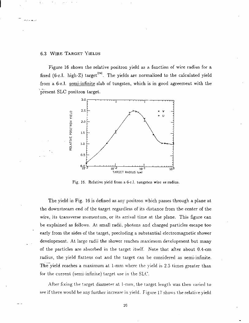
6.3 WIRE TARGET YIELDS

Figure 16 shows the relative positron yield as a function of wire radius for a

fixed (6-r.1. high-Z) target13”. The yields are normalized to the calculated yield

from a 6-r.1. semi-infinite slab of tungsten, which is in good agreement with the

‘$esent SLC positron target.

xv -

TARGET RADIUS km1

Fig. 16. Relative yield from a 6-r.1. tungsten wire ws radius

The yield in Fig. 16 is defined as any positron which passes through a plane at

the downstream end of the target regardless of its distance from the center of the

wire, its transverse momentum, or its arrival time at the plane. This figure can

be explained as follows. At small radii, photons and charged particles escape too

early from the sides of the target, precluding a substantial electromagnetic shower

development. At large radii the shower reaches maximum development but many

of the particles are absorbed in the target itself. Note that after about 0.4-cm

radius, the yield flattens out and the target can be considered as semi-infinite.

The-yield reaches a maximum at l-mm where the yield is 2.5 times greater than

for the current (semi-infinite) target use in the SLC.

After fixing the target diameter at l-mm, the target length was then varied to

see if there would be any further increase in yield. Figure 17 shows the re1atii.e yield

26

I

- I-. . . * -.,

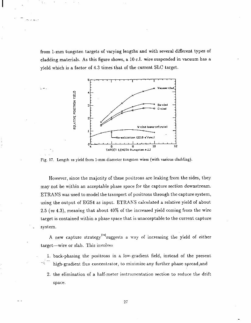
from l-mm tungsten targets of varying lengths and with several different types of

cladding materials. As this figure shows, a lo-r.1. wire suspended in vacuum has a

yield which is a factor of 4.3 times that of the current SLC target.

Fig. 17. Length

v-clad lremmnFmltel

us yield from l-mm diameter tungsten wires (with various cladding).

However, since the majority of these positrons are leaking from the sides, they

may not be within an acceptable phase space for the capture section downstream.

ETRANS was used to model the transport of positrons through the capture system,

using the output of EGS4 as input. ETRANS calculated a relative yield of about

2.5 (VS 4.3), meaning that about 40% of the increased yield coming from the wire

target is contained within a phase space that is unacceptable to the current capture

_ system.

A new capture strategy 13’1suggests a way of increasing the yield of either

target-wire or slab. This involves

1. back-phasing the positrons in a low-gradient field, instead of the present .--

-- high-gradient flux concentrator, to minimize any further phase spread,and

2. the elimination of a half-meter instrumentation section to reduce the drift

space.

27

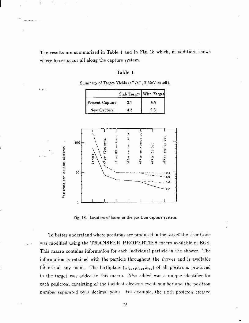
The results are summarized in Table 1 and in Fig. 18 which, in addition, shows

where losses occur all along the capture system.

Table 1

Summary of Target Yields (e+/e-, 2 MeV cutoff)

Fig. 18. Location of losses in the positron capture system

To better understand where positrons are produced in the target the User Code

was modified using the TRANSFER PROPERTIES macro available in EGS.

This macro contains information for each individual particle in the shower. The

information is retained with the part.icle throughout the shower and is available .-- for use at any point. The birthplace (ztag,ytn9, tlag) of all positrons produced

in the target was added to this macro. Also added was a unique identifier for

each positron, consisting of the incident electron event number and the positron

nllmber sepa.rat4 by a decimal point. For example, the sixth positron created

28

by the second incident electron would have an identifier of 2.006. This identifier

was read in with the ETRANS input file (from EGS4) and also output with the

positrons accepted by ETRANS. The ETRANS output was then used as EGS4

input. Namely, the showers were initiated again with the identical random number

seed used to create the rays initially. The identifier of every positron created in 1 -.. the shower was compared with the identifier of the accepted positrons. If they

matched, the location, energy, momentum, etc. were output for analysis. If the

ID’s did not match, the particle was discarded. In this way, it is known during the

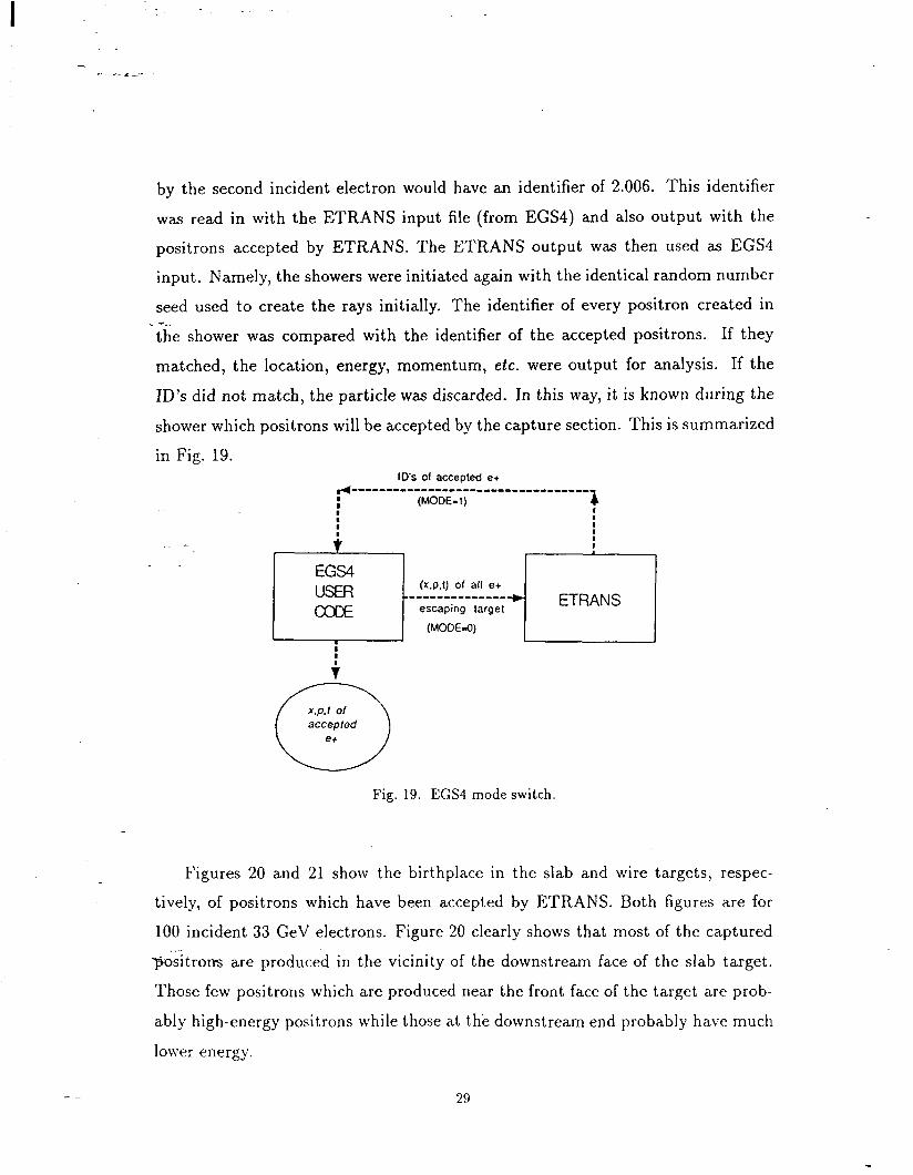
shower which positrons will be accepted by the capture section. This is summarized

in Fig. 19. ID’s of accepted e+

~---------------------------------- : (MODE-l) : t

: !

vJ.t of

0

accepted e+

Fig. 19. EGS4 mode switch.

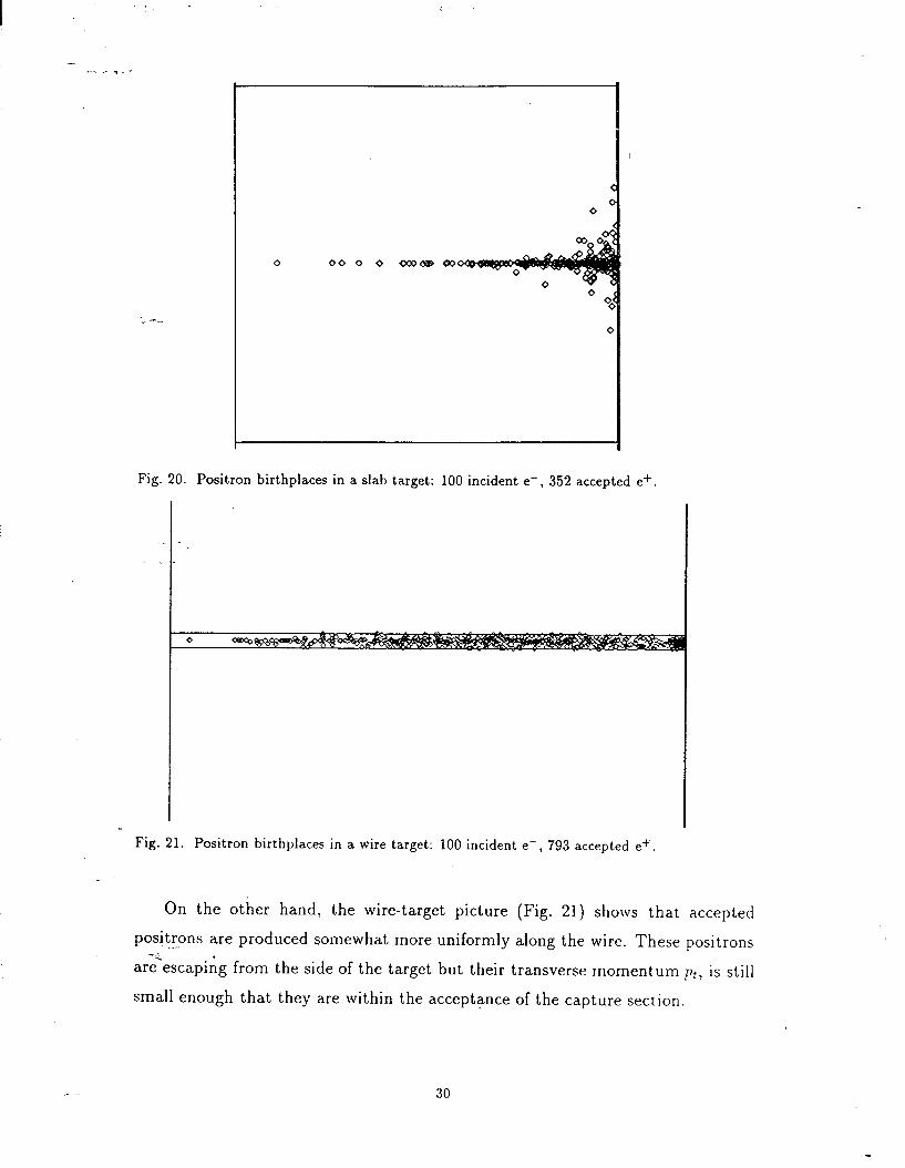
Figures 20 and 21 show the birthplace in the slab and wire targets, respec-

tively, of positrons which have been accepted by ETRANS. Both figures are for

100 incident 33 GeV electrons. Figure 20 clearly shows that most of the captured

-l&trorrs are produced in the vicinity of the downstream face of the slab target.

Those few positrons which are produced near the front face of the target are prob-

ably high-energy positrons while those at the downstream end probably have much

lower energy.

29

0

0 000 0

0 <

Fig. 20. Positron birthplaces in a slab target: 100 incident e-, 352 accepted e+.

Fig. 21. Positron birthplaces in a wire target: 100 incident e-, 793 accepted e’.

On the other hand, the wire-target picture (Fig. 21) shows that accepted positrons are produced somewhat more uniformly along the wire. These positrons ._- are-escaping from the side of the target but their transverse momentum pt, is still

small enough that they are within the acceptance of the capture section.

30

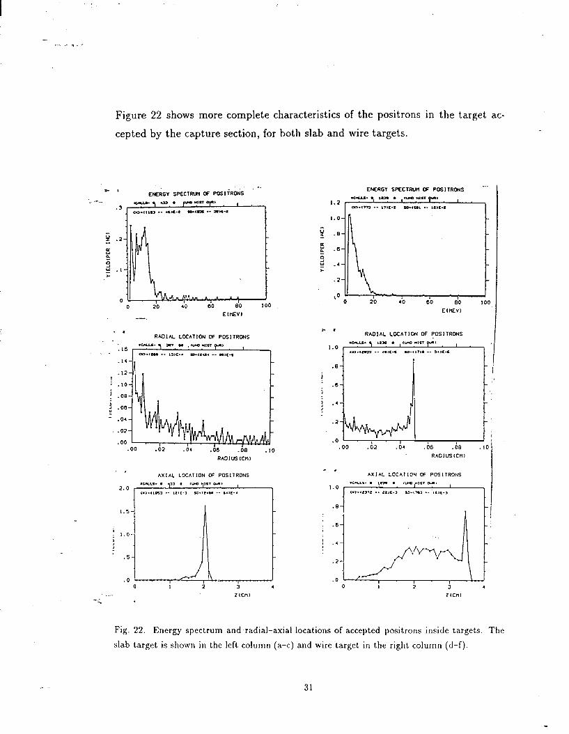
Figure 22 shows more complete characteristics of the positrons in the target ac-

cepted by the capture section, for both slab and wire targets.

! . 12

* .I0

i .OG j

.06 Y - .04

-02

.oo

RAOIVS tCnl

. ENERGY SPECTRUtl OF POSITRONS

RAOIAL LOCATION OF POSITRONS -- ,*a0 . cue q **r a

1.0 ! .

‘*-‘a,, .- .O>L-‘ so-<l71* -- ,.x-s

.oo .02 .04 .iS .ie .Ioi

Fig. 22. Energy spectrum and radial-axial locations of accepted positrons inside targets. The

slab target is shown in the left column (a-c) and wire target in the right column (d-f).

.6

1

RAOlUSlCnl

.4 1 Al\- _ I\ 1 .2-

.O L--y,

0 I 2 3 .

31

6.4 ALTERNATIVE GEOMETRIES

Figure 23 is a plot of the birthplace of 680 positrons inside a semi-infinite

slab target that were accepted by ETRANS, which suggests that perhaps a small- ; -.. diameter, cone-shaped target may enhance the yield. This is reasonable from

a cascade shower viewpoint since the lateral spread of the shower increase as it

develops. This is clearly demonstrated in the SHOWGRAF plots given in Fig. 24

showing particle tracks created inside a 10-r-l. wire target.

Fig. 23. Birthplace of positrons in 6-r.1. slab target which have been accepted by the capture

system. -_ .

32

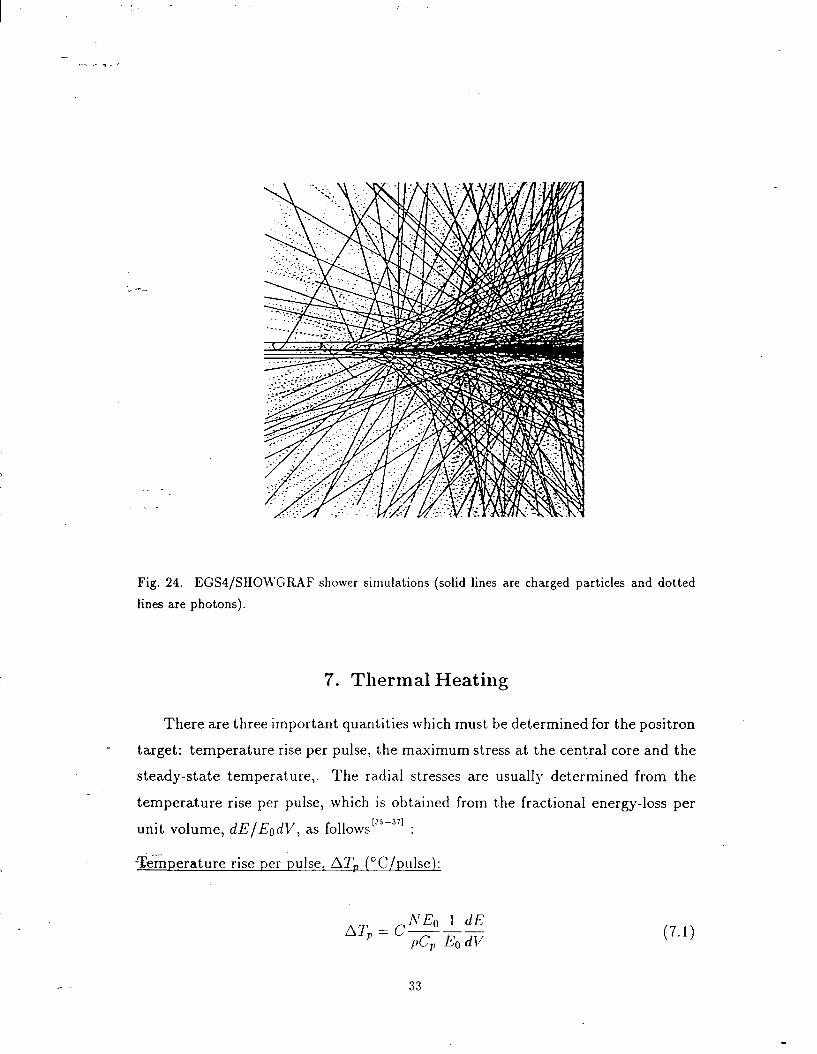
Fig. 24. EGS4/SHO\VGRAF shower simulations (solid lines are charged particles and dotted lines are photons).

7. Thermal Heating

There are three important quantities which must be determined for the positron

target: temperature rise per pulse, the maximum stress at the central core and the

steady-state temperature,. The radial stresses are usually determined from the

temperature rise per pulse, which is obtained from the fractional energy-loss per

unit volume, dE/EodV, as follows[35-371 :

-%%perature rise per pulse, AT,, (‘C/pulse):

NE0 1 dE AT,, zz C------ pCp E. dV

33

(7.1)

where

; -..

p = material density (g/cm3),

Cp = heat capacity M - “;p (cal/g”C),

N = electrons/pulse,

& = incident beam energy (MeV),

A = atomic weight (g/mole),

C = 1.6 x 10-‘3/4.1S4 (cal/MeV).

Maximum Radial Stress (r=Oj, (T, (psi):

Q &AT, cr = 2( 1 - q)

where

VP = Poisson ratio (0.25 to 0.30),

cy = coefficient of thermal expansion (“C-l),

E, = Young’s modulus (psi).

7.1 TEMPERATURE RISE/PULSE

A previously written EGS4 User Code’J81 has been modified to produce the

fractional energy deposition per unit volume, -$-g(r, z), which we will refer to as

the energy-deposition density. This User Code was written to deteimine the pulse

temperature rise in radially-large slabs (e.g., beam dumps, collimators, targets,

etc.). EGS4 produces the energy-deposition density for a h-function beam (i.e.,

pencil beam). The user can write a routine to sample the beam over an appropriate

ci&zbuti.on to obtain the proper beam shape but a large amount of execution time

would be required to get enough statistics in the outer radial bins. What was done

instead was to take the energy-deposition density and convolute it analytically with

a Gaussian function using a method by Ecklund and Nelson IA@1 .

34

I :

The general form for a l-dimensional Gaussian distribution is

; -If we assume that the energy-deposition density of the pencil beam is given by

We(r) f -j$-$ , 0

then the convoluted energy-deposition density is

w&g = f * wo = J f(qvo(s) kc .

For a 2-dimensional Gaussian distribution in radial coordinates (?c = rcos:,

jj = S;sin8),

V-4)

(7.5)

(7.6)

where we have taken 6’ = 0 without loss of generality.

Since the EGS4 output is in the form of a histogram averaged over radial bins, we

have r1+1

We(i) E J

We(r) r dr .

r, .--

The convoluted distribution with the same binning is then

(7.7)

35

where

ri+l rJtl 2lr 1

7rf72(rr+1 - 7-f) JJ J e-+COS8) &j -

(7.9) rl rj 0

. -.. The integral over 8 can be reduced to a modified Bessel function, IO. The dou-

ble integration is done numerically, taking special care (along i = j) to provide

the quadrature routine with an integrand that is not ill-behaved over the bin in

question. The above equation assumes that the energy-deposition density does not

vary significantly over the width of each bin.

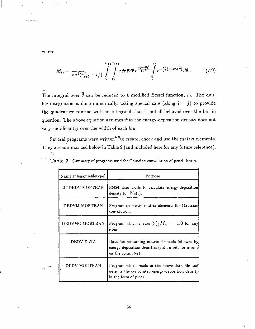
Several programs were written ““to create, check and use the matrix elements.

They are summarized below in Table 2 (and included here for any future reference).

-Table 2. Summary of programs used for Gaussian convolution of pencil beam.

.-- -_

Name (filename-filetype)

UCDEDV MORTRAN

DEDVM MORTRAN

DEDVMC h4ORTRAN

DEDV DATA

DEDV MORTRAN

Purpose

EGS4 User Code to calculate energy-deposition density for We(r).

Program to create matrix elements for Gaussian convolution.

Program which checks Cj hlij = 1.0 for any i-bin.

Data file containing matrix elements followed by energy-deposition densities (i.e., n-sets for n-runs on the computer).

Program which reads in the above data file and outputs the convoluted energy-deposition density in the form of plots.

36

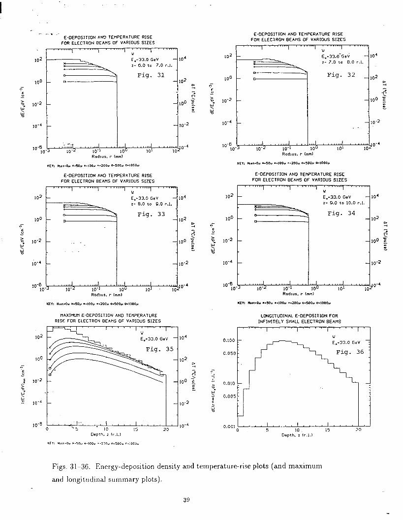
The temperature rise per pulse (and &) for the convoluted beam are shown

in Figs. 25-34 for 1-r.1. to 10-r-l. The maximums are summarized in Fig. 35.

Figure 36 shows the longitudinal energy-deposition density (per r.1.) as a function

of target length (r.1.) for a semi-infinite target (r --t 00).

; -.. The current SLC beam is about 0.6 to 0.8-mm on the slab target. A rather

striking trend can be noticed from these plots: for a beam size between 0.5 to l-mm,

the temperature rise per pulse is almost perfectly flat across the wire radius, but

varies by a factor of lo-20 along the length of the wire. The slab target energy-

deposition density can vary by at least three orders of magnitude over a radius

of a few centimeters, and perhaps a factor of 30-40 from front to back[‘*‘. This

demonstrates a possible advantage of the wire over the slab target. Eq. 7.2 shows

that the radial stresses are directly proportional to the temperature rise per pulse,

., pnd therefore proportional to the energy-deposition density. This demonstrates

why the radial stresses create such a problem for thick targets. While the axial

stresses may be of the same order of magnitude for both targets, there will be a large

difference in the radial stresses. As shown in Figs. 25-34, the wire target seems to

be uniformly heated in the radial direction and may not suffer the effects of large

radial stresses. Remember that 0.5 < g < l-mm and the optimum wire target

diameter is l.O-mm--i.e., the target and beam are about the same size. Therefore,

the radial stresses for the wire target are considered small when compared to the

slab target and are neglected. The important question then becomes: “Mrhnt about

the steady-state temperature?”

37

- .-. .-*..,

E-OEPOSITlW AN0 TE)(PERATLIRE RISE FOR ELECTRON EEMS OF VARmus SIZES

1 I-

102 E.-J%0 Gev - 10’ *- 0.0 to 1.0 r.,.

E-OEWSITIW AND TEWERATURE RISE FOR ELECTRON BEAtiS OF VARIOUS SIZES

, “c . . ..- ..““, ; . ,...,., . . .

E.-33.0 GeV 10’ z- 2.0 10 3.0 I-.,.

IOd 10.

’ ’ * w 10’ lo- 100 10’ ;/$P-’

Rodws. c lwd

EMPOSITION AMI TEHPERATuRE RISE FOR ELECTRON BEArtS OF VARlOwS SIZES

E-OWOS,T,ON AM) TE”PERATURE RISE FOR ELECTRON BEAMS OF VhRIOLtS SIZES

102

100 ” E >o w’

10-Z G

-

E-OEPOSITION AN0 TEWERAWRE RISE FW ELECTRON BEA.nS OF VARIOUS SIZES

, . * . ..,. Ll-vm . . . . * . . “..‘, v . . . . . . . “&/

lo2 !s??b% : t

100 ? k z w- IO.2

E.-33.0 G.V

1

10’ I- 3.0 co 4.0 I-.,.

Fig. 28

:

1o2 P + x .

100 -2 5 i m

t

10‘2

E-OEPOSITION AND TEWERATURE RISE FOR ELECTRON BEAtiS OF VARIO”S SIZES

Figs. 25-30. E nergy-deposition density and temperature-rise plots

38

E-DEPOSITION AND TEf lPERATURE RISE FOR ELECTRON BEAM OF VARIOUS SIZES

, , , . , .,., , , , 1 I . . . . , I , . * . . . . ; . 1 I . .**, q 1 . 1

E,-33.6Ge6 104

I-. .-. L -.i

E-DEPOSITION AN0 TEMPERATURE RISE FOR ELECTRON BEAMS OF VARIOUS SIZES

I . “““‘I - ’ “““1 ’ “““” ’ “““” - - “‘“I !J E,-33.0 GeV 104 z- 6.0 to 7.0 r.1.

Fig. 31 102

2

z- 7.0 to 8.0 r.1.

Fig. 32 1o2 P -4 -5

100 : ;; E

Radius. P (mm1 Radrus. r Imm)

KEY: Past-Or r-50” .-100~ +-200” 0-500~ 0-1000~

E-OEPOSITION AN0 TEMPERATURE RISE FOR ELECTRON BEAtlS OF VARIOUS SIZES

, I I.1 ““, I I II ,,,,( ; I1111 II I I II

102 E.-33.0 GeV 104

E-OEPOSITION AN0 TEf lPERATURE RISE FOR ELECTRON BEAMS OF VARIOUS SIZES

I n 11”“‘1 * b “““I a ’ “““I ’ * “‘ml w 102

100 ? 5 % tt; 10-2

%

10-d

10-6 10

E.-33.0 GeV z- 9.0 to 10.0

Fig. 34 z- 8.0 tc~ 9.0 r.1. 1

Fig. 33 102

2

2

100 g

s

10-2

5 I- Radlut. I- (mm)

KEY: lh*r-ou x-SOLI ClOOV l -2oo” o-500” o-looo”

tlAXItlUfl E-DEPOSITION AND TEf lPERATURE RISE FOR ELECTRON BEAM OF VARIOUS SIZES

LONGITUOINAL E-DEPOSITION FOR INFINITELY SHALL ELECTRON BEAMS

I’ ‘I ‘I m “‘I *‘I - I” m ‘I ,1

“.V”I

0 5 10 15 20 Depth. z lr.1.)

Figs. 31-36. Energy-deposit ion density and temperature-rise plots (and maximum

and longitudinal summary plots).

39

- I-. .-. L _.a

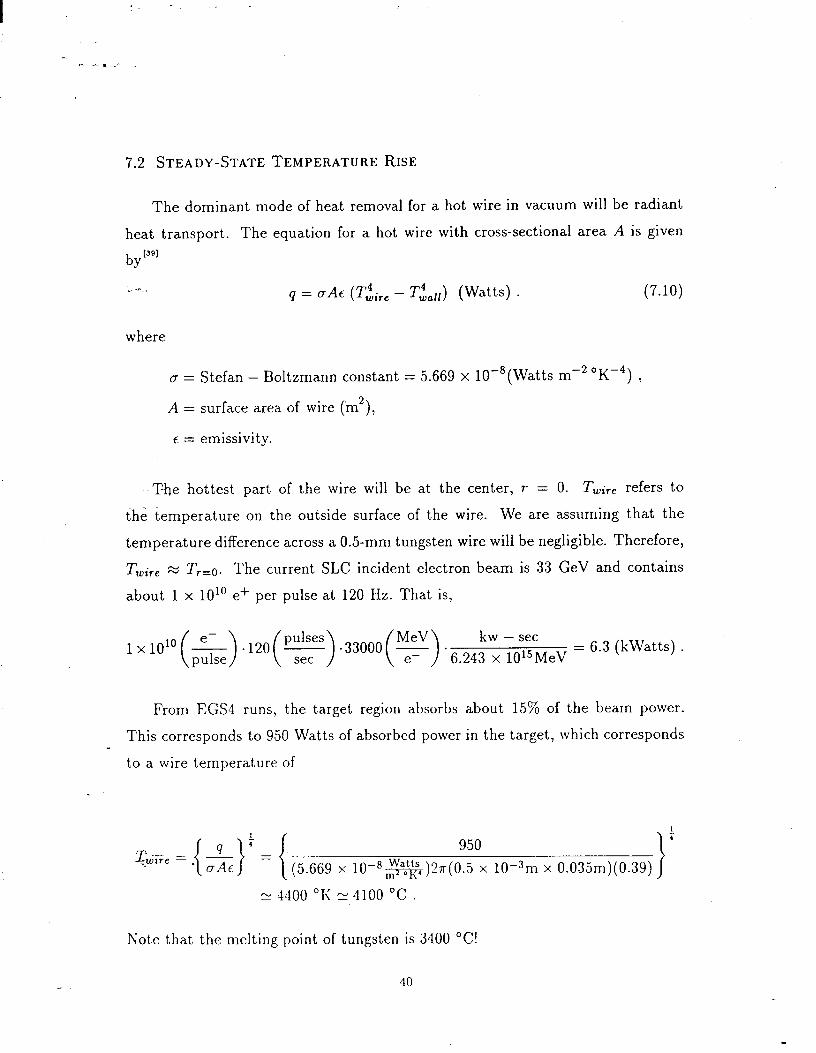
7.2 STEADY-STATE TEMPERATURE RISE

The dominant mode of heat removal for a hot wire in vacuum will be radiant

heat transport. The equation for a hot wire with cross-sectional area A is given

; -.. q = uA~ (~~i,e - Tz,[[) (Watts) . (7.10)

where

c = Stefan - Boltzmann constant = 5.669 x lo-‘(Watts me2 ‘Km4) ,

A = surface area of wire (m2),

c = emissivity.

~The hottest part of the wire will be at the center, r = 0. Twire refers to

the temperature on the outside surface of the wire. We are assuming that the

temperature difference across a 0.5-m m tungsten wire will be negligible. Therefore,

Twire z Tz=o. The current SLC incident electron beam is 33 GeV and contains

about 1 x lOlo e$- per pulse at 120 Hz. That is,

From EGS4 runs, the target region absorbs about 15% of the beam power.

This corresponds to 950 Watts of absorbed power in the target, which corresponds

to a wire temperature of

1. 950 4

(5.669 x lo- 8 sa$, )27~(0.5 x 10m3m x 0.035m )(0.39)

Note that the melting point of tungsten is 3400 “C!

40

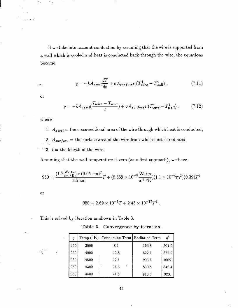
If we take into account conduction by assuming that the wire is supported from

a wall which is cooled and heat is conducted back through the wire, the equations

become

or

q = -kAzsect( Twire 7 Twa”) + OAsurfacec (Tiire - Tia/,) 7 (7.12)

where

1. A zsect = the cross-sectional area of the wire through which heat is conducted,

2. A surface = the surface area of the wire from which heat is radiated,

3. 1 = the length of the wire.

Assuming that the wall temperature is zero (as a first approach), we have

950 = (1.2- J:t$ > 7T (O-O5 cm>2 T + (5.66g x 1o-8 Watts

3.5 cm x)(1.1 x 10-4m2)(0.39)T4

or

950 = 2.69 x 10-3T + 2.43 x lo-r2T4 .

This is solved by iteration as shown in Table 3.

.-- -.;-

Table 3. Convergence by iteration.

q Temp (OK) Conduction Term Radiation Term q’

950 3000 8.1 196.8 204.9

950 4000 10.8 622.1 672.9

950 4500 12.1 996.5 1009.

950 4300 11.6 830.8 842.4

950 4400 11.8 910.8 923.

41

The solution converges at approximately the same temperature as before-

i.e., when we assumed radiative losses only. Note that the conduction term only

accounts for about 1% of the total heat loss. We can therefore conclude that

conduction results in negligible cooling of the wire.

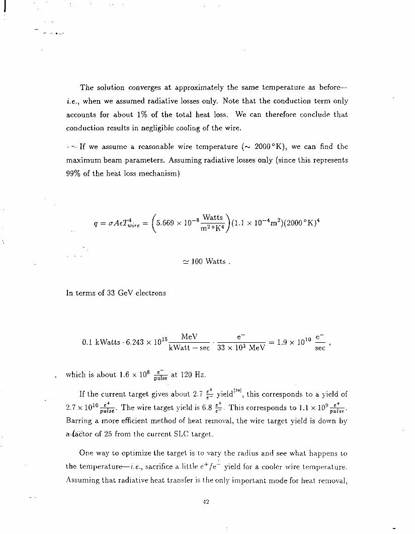
L --. If we assume a reasonable wire temperature (- 2000 OK), we can find the

maximum beam parameters. Assuming radiative losses only (since this represents

99% of the heat loss mechanism)

N 100 Watts .

In terms of 33 GeV electrons

0.1 kWatts. 6.243 MeV e-

x 1015 . - - kWatt - 33 lo3 lMeV 1.9 x 1o’O ) set x 2

_ which is about 1.6 x 10’ & at 120 Hz.

If the current target gives about 2.i $ yieldf3”, this corresponds to a yield of

2.7 x lO’O&. The wire target yield is 6.S $. This corresponds to 1.1 x log&.

Barring a more efficient method of heat removal, the wire target yield is down by

a-&&or of 25 from the current SLC target.

One way to optimize the target is to vary the radius and see what happens to

the temperature-i. e., sacrifice a little e+/e- yield for a cooler wire temperature.

Assuming that radiative heat transfer is the only important mode for heat removal,

42

we know that

(7.13)

or ; --.

(7.14)

We also know that q is proportional to the incident beam power (which is fixed)

multiplied by the fraction absorbed in the wire, f, which varies with the radius.

We can therefore rewrite the above equation as

(7.15)

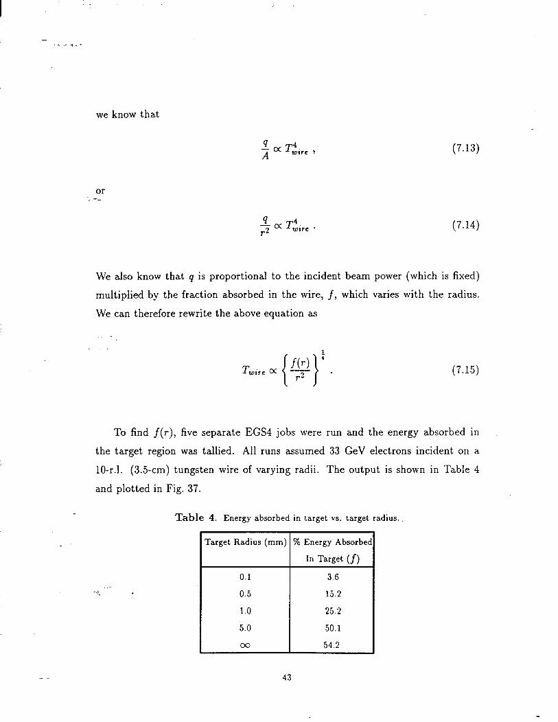
To find f(r), fi ve separate EGS4 jobs were run and the energy absorbed in

the target region was tallied. All runs assumed 33 GeV electrons incident on a

lo-r.1. (3.5-cm) tungsten wire of varying radii. The output is shown in Table 4

and plotted in Fig. 37.

Table 4. Energy absorbed in target vs. target radius..

I Target Radius (mm) % Energy Absorber

In Target (f)

._- -.;- . 0.1 0.1 3.6 3.6

0.5 0.5 15.2 15.2

1.0 1.0 25.2 25.2

5.0 5.0 50.1 50.1

cm cm 54.2 54.2

43

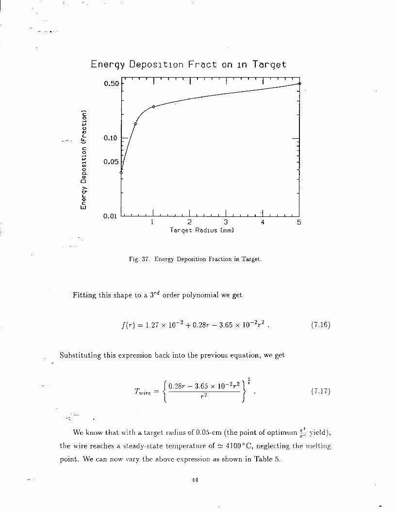
Energy Deposltlon Fract on m Target

0.d ’ ’ ’ ’ ’ ’ ’ ’ ’ ’ ’ ’ ’ ’ ’ ’ ’ ’ ’ ’ ’ ’ ’ 1 2 3 4 5

Tarqet Radius (mm1

Fig. 37. Energy Deposition Fraction in Target.

Fitting this shape to a 3’d order polynomial we get

f(r) = 1.27 x lo-" + 0.2% - 3.65 x 10-2r2 .

Substituting this expression back into the previous equation, we get

(7.16)

(7.17)

..- -.;- .

We know that with a target radius of 0.05-cm (the point of optimum 6 \-ield),

the wire reaches a steady-state temperature of N 41OO”C, neglecting the melting

point. We can now \Tary the above expression as shown in Table 5.

44

- I-. . . L _.a

L -..

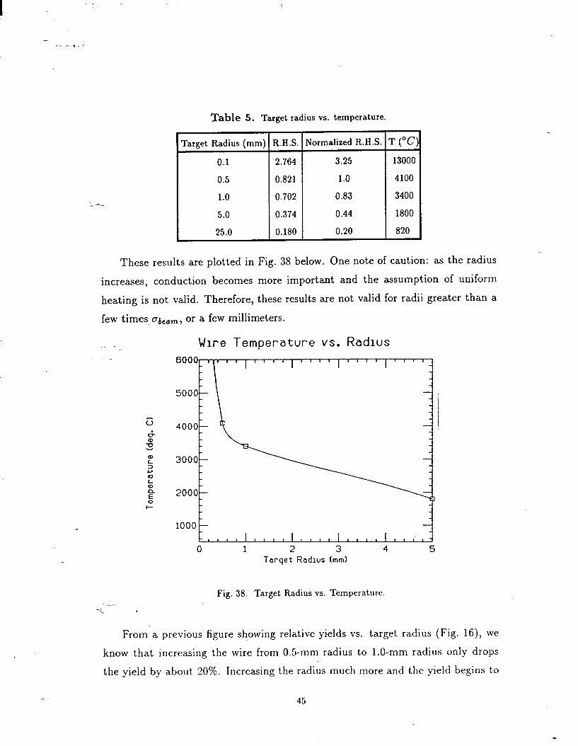
Table 5. Target radius vs. temperature.

Target Radius (mm) R.H.S. Normalized R.H.S. T (“cl

0.1 2.764 3.25 13000

0.5 0.821 1.0 4100

1.0 0.702 0.83 3400

5.0 0.374 0.44 1800

25.0 0.180 0.20 820

These results are plotted in Fig. 38 below. One note of caution: as the radius

increases, conduction becomes more important and the assumption of uniform

heating is not valid. Therefore, these results are not valid for radii greater than a

few t imes C&am, or a few m illimeters.

W ire Temperature vs. Radius

k cl E a

I-

6000

looo~, , , , ] , , , , , , , , ( , , , , , , , ( ,j 0 1 2 3 4 5

Tarqet Radius (mm)

Fig. 38. Target Radius vs. Temperature. ._- -.;- .

From a previous figure showing relative yields vs. target radius (Fig. 16), we

know that increasing the wire from 0.5-m m radius to l.O-m m radius only drops

the yield by about 20%. Increasing the radius much more and the yield begins to

45

approach that of the current slab target. From the figure above we can see that

increasing the wire target radius much beyond the proposed 0.5-mm does not drop

the temperature enough to make a difference.

From the analysis in this section, it appears that severe heating restrictions

gcst be placed on the wire to prevent melting. A better method of heat removal

must be found in order to make the wire target feasible.

8. Discussion

It has been shown that the absolute yield ($) from the proposed wire target

is a factor of 2.5 higher than the current target using the present SLC capture

system, and is a factor of 3.4 higher if an enhanced capture system is employed

(see-Table 1). It h as also been shown that the wire target is severely restricted by *

heat-loss mechanisms when compared to the current target.

To prevent the wire from melting, for example, the intensity of the incident

electron beam must be reduced such that the wire yield is about a factor of 25 below

the current target yield. There are several ideas which should be investigated in

the future and may be used in parallel to enhance the wire target yield, perhaps

enough to make it feasible:

l There are a large number of positrons created off the sides of the wire which

are not captured by the present SLC collector. It may be possible with the

wire target to insert part of it into the flux concentrator. The large transverse

dimensions of the current (slab) target, on the other hand, preclude doing

this (and irery few positrons escape the sides of this target anyways).

r bfiqute heat fins may be placed alon, -.;- c the length of the wire to increase the

conduction surface area. This would also add structural stability to the wire.

l The wire may be placed outside the vacuum system and some kind of con-

vective cooling used.

l The wire could be surrounded by a large graphite region and then surrounded

by copper which could be water cooled. This will eliminate radiative cooling

but increase conduct ive cooling. However, Fig. 17 shows that the yield would

be reduced by almost a factor of two.

..- -; .

4’7

REFERENCES

1. R. Ruth, “Prospects for Next-Generation e + e - Colliders”, SLAC-PUB-4778

(1988).

L “--2. R. Chehab, “Positron Sources”, Laboratoire de 1’Accelerateur Lineaire,

LAL-RT-89-02 (1989).

3. B. Rossi, High-Energy Particles (Prentice-Hall, 1952).

4. W. R. Nelson, H. Hirayamaand D. W. 0. Rogers, “The EGS4 Code System”,

SLAC-265 (1985).

5. Y. S. Tsai, “Pair Production and Bremsstrahlung of Charged Leptons”,

_ &ev. Mod. Phy. 46 (4) (1974) 815.

6. M. Aguilar-Benitez (Particle Data Group), LIReview of Particle Properties”,

Physics Lett. B239 (1990) 111.14.

7. E. Longo and I. Sestili, “Monte Carlo Calculation of Photon-Initiated Elec-

tromagnetic Showers in Lead Glass” Nucl. Instr. Meth. 128 (1975) 283.

8. Private communication with A. Kulikov, SLC Accelerator Physics Group

(1990).

9. E. Freytag, Strahlenschutz an Hochenergiebeschleunigern (G. Braun, Karl-

sruhe, 1972).

10. R. D. Evans, The Atomic Nucleus (McGraw-Hill, 1955).

11. I<. R. Kase and W. R. Nelson, Concepts of Radiation Dosimetry (Pergamon

Press, 1978). .-- -.;- .

12. M. J. Berger and S. M. Seltzer, “Tables of Energ) Losses and Ranges of

Electrons and Positrons”, NASA-SP-3012 (1964).

13. N. F. Mott, Proc. Roy. Sot. (London) Al24 (1929) 425; Al35 (1932) 429.

46

14. R. L. Ford and W. R. Nelson, “The EGS Code System: Computer Pro-

grams for the Monte Carlo Simulation of Electromagnetic Cascade Showers

(Version 3)“, SLAC-210 (1978).

15. A. J. Cook, “Mortran3 Users Guide”, SLAC Computation Research Group

L -.. Technical Memorandum Number CGTM 209 (1983).

16. E. A. Straker, P. N. Stevens, D. C. Irving and V. R. Cain, “MORSECG,

General Purpose Monte-Carlo Multigroup Neutron and Gamma-Ray Trans-

port Code With Combinatorial Geometry”, Radiation Shielding Information

Center (ORNL) Report CCC-203 (1976).

17. Y. Namito, T. M. Jenkins and W. R. Nelson, “ Viewing MORSECG

Radiation Transport With 3-D Color Graphics”, SLAC-PUB-5liO (1990).

., !S: R. Beach, “The Unified Graphics System”, SLAC Computation Research.

Group Technical Memorandom Number CGTM 203 (1985).

19. R. Cowan, “Use of 3-D Color Graphics with EGS”, Comp. Phys. Comm. 45

(1987) 485.

20. R. Donahue and W. R. Nelson, “Distribution of Induced Activity in Tungsten

Targets”, SLAC-PUB-4728 (1988).

21. R. F. Cowan and W. R. Nelson “Producing EGS4 Shower Displays With the

Unified Graphics System”, SLAC-TN-87-3 (1990).

22. T. M. Jenkins, W. R. Nelson and A. Rindi, Monte Carlo Transport of

Electrons and Photons (Plenum Press, 1988).

23. K. R. Shortt, C. I<. Ross, A. F. Bielajew and D. W. 0. Rogers. “Electron

Beam Dose Distributions Near Standard Inhomogeneities”, Phys. Med. Biol. -.;- ‘-- 31 (1986) 235.

24. Bruce A. Faddegon, “Bremsstrahlung of 10 to 30 MeV Electrons Incident on

Thick Targets”. Ph.D. Thesis, Department of Physics, Carleton Universit)

(1990).

49

25. H. L. Lynch, “Documentation of ETRANS Program”, memo from H. L. Lynch

to SLC Positron Source Group (27 October 1988).

26. F. Bulos et al., “Design of a High Yield Positron Source”, SLAC-PUB-3635

(1985).

’ 27. J. E. Clendenin, “High Yield Positron Systems for Linear Colliders”, SLAC-

PUB-4743 (1989).

28. J. E. Clendenin et al., “SLC Positron Source Startup”, SLAC-PUB-4704

(1988).

29. S. Ecklund, “Positrons for Linear Colliders”, SLAC-PUB-4484 (1987).

30. J. E. Clendenin, S. D. Ecklund and H. A. Hoag, “The High-Gradient S-

Band Linac for Initial Acceleration of the SLC Intense Positron Bunch”,

.,~ -- SLAC-PUB-5049 (1989).

31. A. F. Bielajew, D. W. 0. Rogers, “PRESTA - The Parameter Reduced

Electron-Step Transport Algorithm”, Nucl. Instr. Meth. Bl8 (1987) 165.

32. A. F. Bielajew, R. Mohan and C. Chui, “Improved Bremsstrahlung Photon

Angular Sampling in the EGS4 Code System”, NRCC-PIRS-0203 (1989).

33. H. W. Koch and J. W. Motz, “Bremsstrahlung Cross-section Formulas and

Related Data”, Rev. Mod. Phys. 31(4) (1959) 920.

34. M. James, R. J. Donahue, R. Miller and W. R. Nelson, “A New Target Design

and Capture Strategy for High-Yield Positron Production in Electron Linear

Colliders”, SLAC-PUB-5215 (1990).

35. H. DeStaebler, “Temperature Calculations for the Positron Target”, SLC

Single Pass Collider Memo CN-21 (1980).

-$6.- H. DeStaebler, “Calculations for Positron Target Test in ESA” SLC Single

Pass Collider Memo CN-23 (19SO).

.

37. H. DeStaebler, “More Calculations for Positron Target Test in ESr\” SLC

Single Pass Collider Memo CN-24 (19SO).

50

38. S. Ecklund and W. R. Nelson, “Energy Deposition and Thermal Heating in

Materials Due to Low Emittance Electron Beams”, SLC Single Pass Collider

Memo CN-135 (1981).

39. J. P. Holman, Heat Transfer (McGraw-Hill, 1986).

51

ACKNOWLEDGMENTS

I would like to express my thanks to Dr. Ralph Nelson of the Radiation Physics

Group at the Stanford Linear Accelerator Center who has acted as an on-site

-advisor to this work. It was his imagination and hard work which led to this

project. I wish to thank him for the many days (and nights) he put aside for me

in his busy schedule. He has given me much encouragement and serves as a source

of inspiration.

I also wish to express my thanks to Dr. Jose Martin of the University of Lowell

for further improving the work. He has helped make this effort possible across three

thousand miles.

52