Embed Size (px)
Citation preview

3363
AAS 20-481
HIGH-FIDELITY MODELING AND VISUALIZING OF SOLAR RADIATION PRESSURE: A FRAMEWORK FOR
HIGH-FIDELITY ANALYSIS
Leandro Zardaín,* Ariadna Farrés,† and Anna Puig‡
Solar Radiation Pressure (SRP) is the force produced by the impact of sunlight photons on the surface of the spacecraft. This extra force, despite being small, plays an important role on trajectory design and orbit determination. In this pa-per we present an open-source tool that enables the user to compute high-fidelity approximations of SRP accelerations for a given spacecraft using ray-tracing techniques. The tool also allows the user to compare between different fidelity levels and different models like the N-plate or the cannonball finding a trade-off on the SRP accuracy between computation time and accuracy.
* Student, Universitat Politecnica de Catalunya, Carrer de Jordi Girona 1, Barcelona, Spain. E-mail: [email protected]. † Dr., NASA/Goddard Space Flight Center, University of Maryland Baltimore County. 1000 Hilltop Circle, Baltimore, MD 21250, USA. E-mail: [email protected]. ‡ Prof., Universitat de Barcelona, Gran Via de les Corts Catalanes 585, Barcelona, Spain. E-mail: [email protected].
INTRODUCTION
Solar Radiation Pressure (SRP) is the force exerted on a spacecraft by the exchange in momenta
between sunlight and the surface of the spacecraft. The incident sunlight will be absorbed and
reflected by the different components on its surface, where the rate of absorption and reflection
will depend on the surface materials. The magnitude and direction of the acceleration due to SRP
will depend on the spacecraft’s attitude and the reflectivity properties of the surface materials. This
acceleration can be hard to determine for spacecrafts with a complex shape, as it is highly dependent
on the orientation of the spacecraft with respect to the Sun-spacecraft line. In this case, raytracing
techniques are ideal to trace the sunlight and its multiple reflections on the surface of the spacecraft
and provide a good approximation of SRP acceleration for a given attitude.
Despite being a small perturbation, SRP plays an important role in many applications. For ex-
ample, in Libration point missions like the James Webb Space Telescope (JWST) and the Roman
Space Telescope (previously know as the Wide Fields InfraRed Survey Telescope (WFIRST)), SRP
due to their large area to mass ratio is the fourth most relevant perturbation after the gravitational
attraction of Earth, Sun and Moon. Hence it must be accounted for during maneuver planning for
station-keeping and orbit determination (OD). In interplanetary missions like Mars Atmosphere and
Volatile EvolutioN (MAVEN) or Rosetta, where the probes have large solar panels, accurate model-
ing of SRP improves OD errors and mission plans. The Lunar Reconnaissance Orbiter (LRO) uses
a high-fidelity SRP model to improve their OD solutions. Finally, one of the most clear examples
where SRP is relevant are spacecraft orbiting small bodies, as is the case of OSIRIS-REX, where
SRP is the second most dominant force acting on the spacecraft.

3364
Having an accurate approximation of the SRP accelerations on a spacecraft for different attitude
profiles improves the trajectory design, maneuver planning and orbit determination. For this reason
different authors1–5 have proposed different ways to approximate and model this acceleration for
different space applications. Using raytracing approaches is the best way to produce high accuracy
approximations of SRP, as one can trace the path of light rays and compute the force produced by the
first, second and third impacts of the sunlight on the surface of the spacecraft. The main drawback
of this approach is the high computational cost, especially if we account for multiple impacts. In
order to improve the computation speed instead of using the computers Central Processing Unit
(CPU) one can take advantage of the Graphical Processing Unit (GPU) to parallelize part of the
computation, drastically reducing the computational cost.
This paper presents an open-source framework that allows the user to upload the information on
the spacecraft shape and reflectivity properties via a Computer-Aided Design (CAD) model, and
compute a high-fidelity approximation of SRP accelerations using raytracing techniques. The user
can choose from an interactive menu of spacecraft information (shape and reflectivity properties
from an input file) and the type of analyses to perform. The framework supports different meth-
ods/models to compute the SRP force for different attitude configurations using both the CPU and
GPU, enabling the user to choose the level of accuracy for the computation. The framework also
allows the user to visualize the SRP force directions together with the spacecraft as this one rotates
around an arbitrary axis. The user can also choose to compute the SRP force for a grid of azimuth
and elevation angles, producing a table that can be visualized and stored as a text file. The table
of SRP forces allows users to include high-fidelity SRP as a force model in their simulation envi-
ronment. The text files generated by the framework can be used with the General Mission Analysis
Tool (GMAT)6 to perform orbit simulations. Moreover, the framework allows analysts to compare
different levels of approximation between the classical lower fidelity SRP models (cannonball and
N-plate) in order perform a trade-off between accuracy and computational cost.
The different models included in our framework are in increasing order of fidelity: cannonball,
N-plate, raycast and raytrace, where the raycast and raytrace methods have been implemented using
both the CPU and GPU in order to compare their performance and accuracy. The simplest approach
is the cannonball model, where the spacecraft’s shape is approximated by a sphere, having the
SRP acceleration along the Sun-spacecraft direction and a fixed magnitude which only depends
on the spacecraft’s area-to-mass ratio and reflectivity properties. An intermediate approach is the
N-plate model, where the spacecraft is approximated by N flat plates representing the different
spacecraft components, each one with a different size, orientation relative to the Sun-spacecraft line
and reflectivity properties. The N-plate model accounts for the spacecraft attitude, but does not
consider possible self-shadowing between the different plates or the second order impacts of the
incident light on the spacecraft surface. The raycast approach takes into account the shape of the
spacecraft and computes which parts of the spacecraft are directly illuminated by the sunlight for
a given attitude in order to determine the SRP acceleration. The spacecraft shape is provided by a
CAD model, up to a certain level of fidelity, which also has information on the reflectivity properties
of the different components. Finally, the raytrace approach can be considered an improvement on
the raycast approach, as it also accounts for the impact on the spacecrafts surface of the reflected
sunlight rays and the scattering of these sunlight rays due to diffusion.
This paper is structured in the following way: Section 1 gives an overview on how SRP ac-
celerations can be modeled. Section 2 focuses on the raycast and raytrace models, giving a brief
description of their implementation and how to use the GPU to improve their performance. Section
3365
3 describes the framework that has been developed, giving an overview of its main options and
how to use them. Finally, some tests to validate the framework and evaluate its performance and
accuracy are included in Section 4.
BACKGROUND ON SOLAR RADIATION PRESSURE MODELING
The Solar Radiation Pressure (Psrp) exerted on an object at a distance R from the Sun is given
by:7, 8
Psrp =P0
c
(R0
R
)2
= 4.57× 10⁻⁶(R0
R
)2
[N/m2],
where P0 = 1, 367 W/m2 is the solar flux at 1 AU, c = 299, 792, 458 m/s is the speed of light and
R0 is the Sun-Earth mean distance. Notice that this force is inversely proportional to the distance to
the Sun.
Classical optics uses two approaches to describe the behavior of the light: geometrical optics and
physical optics. In the first case, the propagation of the light is defined in terms of rays, straight
lines that follow the laws of reflection and refraction when traveling through a media. In the case of
physical optics, light is considered as an electromagnetic wave and could model some other effects
such as diffraction and interference. In this case, we considered the light under a geometric optics
approximation commonly used in computer graphics. Kajiya9 defined the Rendering equation to
model the total amount of light leaving a point as a function of the incoming light (emitted and
reflected). Several approaches to solving the equation, such as finite element methods and Monte
Carlo approaches have been proposed (path tracing, photon mapping, and Metropolis light transport,
among others). One of the simplest algorithms to sample this integral is the raytracing algorithm.10
This algorithm constructs an image by tracing imaginary rays from an observer through each pixel,
and computing the colors at each pixel as a result of the incoming radiance of the objects that the
ray hits. There are several raytracing approaches but we focused on two classical versions: the
raycasting algorithm,11 that only considers the closest object that the ray hits from the eye, and the
recursive raytracing algorithm10 that takes into account the bounced rays generated when a ray hits
a surface.
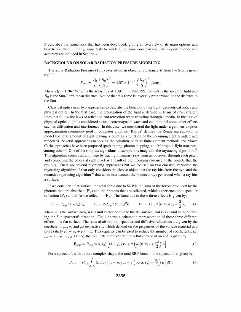
If we consider a flat surface, the total force due to SRP is the sum of the forces produced by the
photons that are absorbed (Fa) and the photons that are reflected, which experience both specular
reflection (Fs) and diffusive reflection (Fd). The force due to these three effects is given by:
Fa = PsrpA〈n, rs〉rs, Fs = 2PsrpA〈n, rs〉2n, Fd = PsrpA〈n, rs〉(rs + 2
3n), (1)
where A is the surface area, n is a unit vector normal to the flat surface, and rs is a unit vector defin-
ing the Sun-spacecraft direction. Fig. 1 shows a schematic representation of these three different
effects on a flat surface. The rates of absorption, specular and diffusive reflections are given by the
coefficients ρa, ρs and ρd respectively, which depend on the properties of the surface material and
must satisfy ρa + ρs + ρd = 1. This equality can be used to reduce the number of coefficients, i.e.
ρa = 1− ρs − ρd. Hence, the total SRP force exerted on a flat surface of area A is given by:
Fsrp = PsrpA〈n, rs〉[(1− ρs) rs + 2
(ρs〈n, rs〉+ ρd
3
)n]. (2)
For a spacecraft with a more complex shape, the total SRP force on the spacecraft is given by:
Fsrp = Psrp
∫∂Ω
〈n, rs〉[(1− ρs) rs + 2
(ρs〈n, rs〉+ ρd
3
)n]dΩ, (3)

3366
Figure 1. Schematic representation of the force due to absorption (left), specularreflection (middle) and diffusive reflection (right) on a flat surface.
where ∂Ω is the boundary of the surface defining the spacecraft’s visible shape, and dΩ is the
element of area. Note that the reflectivity properties ρa, ρs and ρd vary along the surface ∂Ω.
Hence, depending on the complexity of the shape and diversity of materials of the spacecraft, this
integral can be hard to estimate.
In practice one has to make some assumptions and simplifications in order to approximate this
function. In the literature we find three different approaches: a) cannonball model (simplest) that
approximates the spacecraft by a sphere; b) N-plate model (intermediate) that approximates the
spacecraft by flat plates; c) Finite Element model (high-fidelity) that uses a CAD model to approxi-
mate the spacecraft and raytracing techniques to find the illuminated components of the spacecraft
and compute the total SRP acceleration.
Cannonball model
The cannonball model is the simplest way to approximate the SRP acceleration and is com-
monly used in preliminary mission analysis as it gives a first order approximation on the impact of
SRP. This model considers the SRP acceleration to be constant along the Sun-spacecraft direction,
where the acceleration magnitude depends on the area-to-mass ratio and a reflectivity coefficient Cr.
Which comes from approximating the shape of the spacecraft by a sphere with constant reflectivity
coefficients along the surface and integrating Eq. 3. The total SRP acceleration is given by:
asrp =PsrpCrA
msatrs [m/s2], (4)
where A is the projected area, msat is the spacecraft mass, rs is the normalized Sun-spacecraft
direction and Cr ∈ [1, 2] accounts for the reflectivity properties. The value Cr is hard to predict
but one can consider it to be approximately Cr = (1 + ρs). Where Cr = 1 indicates that all the
sunlight is absorbed, and Cr = 2 when all the light is reflected and twice the force is transmitted to
the spacecraft. Note that the SRP acceleration is proportional to the spacecraft area-to-mass ratio,
and the acceleration units are m/s2 if the projected area A and the spacecraft mass msat are given in
m2 and kg respectively.
N-plate model
The N-plate model is an intermediate approximation that accounts for the variations of the SRP
acceleration due to changes on the spacecraft attitude, providing a more accurate approximation
which has been used during mission operations. Here, the shape of the spacecraft is approximated

3367
Figure 2. Left: schematic representation of an N-plate model for a spacecraft. Right:illumination conditions for one of the plates.
by a collection of flat plates, each of them having different reflectivity properties, allowing the SRP
magnitude to vary depending on the spacecraft’s orientation with respect to the Sun-spacecraft line.
Each flat plate (Πi) is defined by the normal vector to its surface ni, the plate’s surface area Ai,
and the reflectivity properties (ρis, ρid), recall that ρia = 1− ρis − ρid (see Fig. 2 left). Using Eq. (2)
one can derive that the SRP acceleration for a collection of N-plates is given by:
asrp =Psrp
msat
N∑i=1
(Ai cos θi
[(1− ρis)rs + 2
(ρis cos θi +
ρid3
)ni
]H(θi)
)[m/s2], (5)
where cos θi = 〈ni, rs〉, and H(θi) is the illumination condition for the i-th plate:
H(θi) =
{1 if cos θi < 0,0 if cos θi ≥ 0.
Notice that a flat plate only reflects on one side, hence if the light hits the back side of a plate its
SRP should not be counted. This is accounted for by the illumination condition H(θ). If the normal
vector to the plate (ni) is defined so that it points out from the reflective face (see Fig. 2 right) and
rs is Sun-spacecraft ray, the face is illuminated by the ray if 〈ni, rs〉 = cos θ < 0. Again, the
acceleration units are m/s2 if the plate’s area A and the spacecraft mass msat are given in m2 and
kg respectively.
The only disadvantage of this approximation is that it does not take into account possible auto
occultation between the different plates. This is because the definition used for each plate does not
carry information on their relative position. Hence, if there is an occultation between two plates, the
user needs to manually eliminate one of the plates for certain attitudes to account for it.
Finite Element
In order to account for the auto occultation between the different components of a spacecraft
Ziebart1, 12, 13 was the first to propose the use of raytracing techniques to determine which parts
of the spacecraft are illuminated by the sunlight for a given orientation relative to the sunline. In
his work Ziebart proposed to approximate the spacecraft structure using simple geometric shapes
(cubes, cylinders, spheres, ...), and use raytracing to determine the objects that where illuminated

3368
Figure 3. Left: schematic representation of a spacecraft using triangles. Right:schematic representation of a pixel array used to determine the illuminated parts of aspacecraft.
for a given attitude orientation and integrate Eq. 3 to find the total SRP acceleration. In the literature
we find other authors that have proposed the same approach. For instance Rivers14, 15 also uses
raytracing to compute different surface forces like SRP and Thermal Recoil Pressure (TRP) on
the Rosetta probe. On the other hand, Kenneally5, 16, 17 proposed different GPU based approaches
using OpenCL and geometric shaders to compute SRP acceleration during the propagation of the
spacecraft through its trajectory. Our approach focuses on the use of vertex and fragment shaders
to parallelize the SRP computations for different orientations of the spacecraft. Additionally, our
framework allows us to validate the accuracy of the proposed optimizations finding the best trade-off
between the accuracy and the time performance between the different methods.
The general idea is to approximate the spacecraft by simple geometric objects by Finite Elements,
where the simplest way is the use of triangles or polygons (see Fig. 3 left). This approximation can
be done manually or using a CAD software. Then a plane perpendicular to the sunline rs at a certain
distance from the spacecraft is built, commonly known as the pixel-array, which represents the solar
flux (see Fig. 3 right). Finally we take a grid of points in this pixel-array and from each point on the
grid a ray is projected along rs to the spacecraft. The parts of the spacecraft that are intersected by
these rays corresponds to the illuminated surfaces. It is easy to check if the rays intersect any of the
triangles/polygons on the spacecraft’s surface using simple algebra. Using a similar approach one
can also check the second and third order reflections of the solar rays on the spacecraft.
The main drawback of this finite element approximation is the computational cost. In order to
have an accurate approximation we need a large number of points on the pixel-array that approx-
imates the solar flux, increasing the computational time exponentially. Hence, it is not advisable
to compute this simultaneously during an orbit propagation with GMAT, AGI’s Systems Tool Kit
(STK) or any other orbit simulation software. Hence, the SRP acceleration is usually computed be-
fore hand for a set of predetermined attitudes configurations, and polynomial interpolation is used
to during an orbit propagation to approximate the SRP acceleration for any intermediate attitude.
HIGH-FIDELITY MODELING OF SRP
As mentioned in the previous section, for a more accurate approximation of SRP the main goal
is, on the one side, to model the light paths more realistically, and on the other side, to use a more
detailed representation of the spacecraft’s surface. This can be done using computer visualization

3369
techniques and the use of the GPU instead of the CPU to help speed up the computational time
which is the real bottle-neck in these types of computations.
We propose to use both algorithms to approximate the SRP considering the Sun as the observer,
and compute the SRP-values at each pixel of the image by tracing rays from the Sun to the scene
where the spacecraft is located. The total SRP acceleration will be computed as the total amount
of SRP-values of all the pixels of the image. However, these computations tend to be costly and
time consuming when using just the CPU. Therefore, taking advantage of the capabilities of the
GPU18 can help reduce the computational time, hence we also present a GPU-based version of both
approaches.
Regarding the spacecraft modeling, we use a CAD model composed of a mesh of triangles,
where each triangle stores information about its three vertices, its normal direction, and its material
properties (ρs, ρd) that define the light behavior. In this way, we can model different parts of the
spacecraft with different materials, being more or less reflective, more or less diffuse, etc. Initially,
we consider that the spacecraft does not have any transparent parts and is totally opaque.
In the following sections, we define the main differences between the raycasting and raytracing
approximations, and their GPU optimizations, respectively.
Raycasting versus Raytracing Algorithms
Let us assume that the Sun is the observer of the scene, thus we create a grid of Nx × Ny cells
over a plane perpendicular to the Sun-spacecraft direction, sized to contain the projection of the
spacecraft along that direction. Then, for each cell of this grid, a ray is casted to check whether it
intersects with any triangle of the spacecraft’s surface. We will use a pixel array to represent this
grid of cells.
In the raycasting version, we just consider a ray per cell (called primary ray) and find the closest
triangle of the spacecraft’s mesh to the Sun that is hit by the primary ray (see Fig. 4 left). Then for
each element in the grid, we compute the local SRP acceleration as:
asrp cell =PsrpAcell
msat〈n, rs〉
[(1− ρs)rs + 2(ρs〈n, rs〉+ ρd
3)n
], (6)
where Acell is the size of the cells in the perpendicular plane.
Note that, by considering really small cells, the addition of the contribution of each cell approxi-
mates an integral and thus the formula of the SRP acceleration can be expressed as:
asrp =PsrpA
msat
∫∂Ω
(〈n, rs〉
[(1− ρs)rs + 2(ρs〈n, rs〉+ ρd
3)�n])
dΩ, (7)
where A is the addition of the cell’s areas which is constant. As mentioned previously, Nx, Ny
are two integers defining the size of the grid and ∂Ω corresponds to the illuminated surface of the
spacecraft. As for the other models the acceleration units are m/s2 if the spacecrafts size in the CAD
model and its mass msat are given in m2 and kg respectively. Algorithm 1 shows the main strategy
of this approach.
In the raytracing algorithm, we also consider secondary rays modeling specular and diffuse re-
flections recursively (see Fig. 4 right). We consider the specular reflections as ‘perfect’ reflections,
which means that the computation of the specular reflection is deterministic: i.e. for the same input

3370
(the incident ray and the surface normal), the procedural will always give the same reflected direc-
tion. Instead, the evaluation of the diffuse reflections are done by casting several secondary rays
in random directions. Thus, we developed two versions of the raytracing method depending on the
number of secondary rays that bounce at each intersection. We refer to single-scattering when we
cast just one ray at each hit, meanwhile we talk of multiple-scattering when more than one rays are
generated.
In summary, an incident ray can bounce into different types of rays: a specular ray, computed
as the reflected direction which depends on the incidents ray direction on the surface normal; and
a set of one or more diffuse rays casted into random directions. Each ray contribution will be
weighted with the corresponding specular and diffuse material properties of the spacecraft. So, the
SRP acceleration of the raytracing approximation is a recursive function defined as:
asrp =PsrpA
msat
∫∂Ω
(〈n, rs〉
[(1− ρs)rs + 2(ρs〈n, rs〉+ ρd
3)n
])dΩ
+ ρsasrp(reflectspecular(rs)) +1
kρd
k∑i=1
asrp(reflectdiffuse(rs)).(8)
Algorithm 2 explains the multi-scattering strategy. It should be noted that this approximation is
more accurate, however, depending on the spacecraft model, it can became more time consuming
due to its exponential cost in time and memory.
Figure 4. Schematic representation of raycasting (left) and raytracing (right). Foreach cell of the grid, a ray is cast from the Sun and traced to the spacecraft to checkif there is an intersection. In the raytrace for each ray that reaches the spacecraftsurface, secondary rays are casted.
GPU-based Optimizations
To obtain interactive times in our SRP computations, we propose two GPU-optimizations related
to raycasting and raytracing based approaches. In the former one, where we want to obtain at each
pixel of the grid the contribution of the projected triangles of the spacecraft, we apply a ZBuffer
algorithm. In this case, the mesh of triangles is sent to the GL-pipeline, via the Vector Array Objects
(VAO). In the fragment shader the partial SRP value related to each pixel is computed using Eq. 6.

3371
Data: rs, Nx, Ny
Result: asrpFunction Raycast(rs, Nx, Ny):
T = # (flat surface)
asrp = 0for cell ∈ grid(Nx, Ny) do
r = ray(cell, rs)
t = getClosestCollidedFlatSurface(r)
if t ∈ {1, . . . , T} thenasrp = asrp +
PsrpAcell
msat
(〈nt, rs〉[(1− ρts)rs + 2(ρts〈nt, rs〉+ ρt
d
3 )nt])
endendreturn asrp
Algorithm 1: Raycast algorithm.
At the end, we recover the frame buffer with all the partial values, and compute the total SRP value
in the CPU.
In the latter case, the raytracing approach, we use a variant of the rendering technique proposed
by Christen.19 In this case, we send in one single pass the faces of the bounding box of the spacecraft
to activate the corresponding fragment shaders, and use 1-D textures to send the rest of parameters
(such as the mesh of triangles of the spacecraft, the set of normals, ...) to the fragment shader.
There, each fragment performs a cast of a ray (primary ray) and checks if the ray intersects with any
face of the model and if so, it gets the triangle with the closest intersection. The closest intersection
obtained belongs to the surface of the spacecraft and from this point, secondary rays can be casted
(considering specular or diffuse reflections). Each fragment shader computes the partial value (see
Eq. 8) using the recursive algorithm. At the end, we recover the frame buffer as above and compute
the total value of SRP in the CPU.
The GPU based versions decrease the computational time, considerably. However, the main
drawback of the GPU-based version is the precision of the data to be sent to the GPU. For instance,
textures contain values codified as floats instead of doubles, and the accuracy of the SRP computa-
tion could decrease. This will be analyzed in the next sections.
THE SRP FRAMEWORK
The main goal of this project was to develop a framework that allows the simple computation
and visualization of high-fidelity approximations of SRP accelerations. The information on the
spacecraft shape and material reflective properties is introduced through two text files. The user is
then able to chose between three different options:
(a) Live visualization of the SRP accelerations. This feature allows the user to interactively see
how the direction the SRP acceleration and its magnitude vary as we change the spacecrafts
attitude.
(b) Compute SRP accelerations for a mesh of azimuth and elevations around the spacecraft using
any of the above methods. This can be either visualized on a graph or download the results
on a text file which can be used in GMAT, STK or any other flight dynamics software to
incorporate SRP perturbations on the force models.

3372
Data: rs, Nx, Ny
Result: asrpFunction Raytrace(rs, Nx, Ny):
asrp = 0 for cell ∈ grid(Nx, Ny) doasrp = asrp + Raytrace MS (cell, rs, 0)
endreturn asrp
Function Raytrace MS(cell, �rs, numReflections):T = # (flat surfaces)
if numReflections == MAX REFLECTIONS thenreturn (0,0,0)
endforce = 0
r = ray(cell, rs)
[t, hitpoint] = getClosestCollidedFlatSurface(r)
if t ∈ {1, . . . , T} thenforce =
PsrpAmsat
(〈nt, rs〈[(1− ρts)rs + 2(ρts〈nt, rs〉+ ρtd
3 )nt]) +
+ ρts Raytrace MS (hitpoint, reflectspecular(rs), numReflections+ 1) +
+ 1k
∑k ρ
td Raytrace MS (hitpoint, reflectdiffuse(rs), numReflections+ 1)
endreturn force
Algorithm 2: Raytrace multiple-scattering algorithm
(c) Compare between different SRP models. This feature is interesting as it allows the user to
see the differences between different fidelity approximations for the spacecraft representation
(CAD model) or the SRP approximation using different methods (raycast vs raytrace with
single or multiple scattering).
The GUI window design
We have designed a GUI that allows the user to input the spacecraft information, choose a method
to compute the SRP acceleration and the type of visualization between the three options described
above. Fig. 5 shows the main window of this framework.
The first step is to load the spacecraft information and set its basic properties, which is found
in the top of the main window. The user must enter two text files, one with the spacecraft object
(*.obj) and another with the material properties (*.mtl), and finally the spacecraft mass (see
block 1 in Fig. 5).
The second step is to choose the method the user wants to apply (see block 2 in Fig. 5). Once a
method is selected a short explanation on the method appears. In addition, the window will display
the parameters that the user can tune for the computations. For each user-editable parameter (which
are specific for each method), the icon with the letter ‘i’ displays a description of the parameter and
how it is used in the computations. Furthermore, two properties of the selected method are shown:
the accuracy and the performance of the selected method in comparison to the other ones. This is
represented as a set of little green boxes in order to make it easier to understand by the users.
The final step is to choose between the three different options depending on the type of analyses
required by the user (see block 3 in Fig. 5). As detailed before these options are: Visualize Satellitewhich allows the user to visualize the spacecraft and SRP accelerations live; Visualize Graphics

3373
which allows the user to compute the SRP accelerations for a mesh of azimuth and elevations, and
Compare Graphics that allows the user to compare the SRP accelerations of the same spacecraft
using different methods. We note that for this last option, the framework only allows one to compare
methods that have previously been computed with the Visualize Graphics option.
Figure 5. Main window of the framework.
Input Parameters
As mentioned above, the spacecraft information is loaded with two text files. The first file *.obj,
uses the Wavefront format* and contains information on the spacecraft geometry and type of mate-
rials. The file contains a list of all the vertices in the triangle approximation as well as how these
vertices relate to each other and what material is associated with each triangle. This is a simple
ASCII file that can be generated with many different CAD packages. The second file, a *.mtl, is
also an ASCII file and has to be manually generated by the user. This file contains the name of the
different materials in the *.obj file and their reflectivity coefficients (ρs, ρd).
We must mention that if we choose to compute the SRP accelerations using the cannonball model
this input file is only used for visualization purposes but not for the computation of SRP accelera-
tions, and if we choose to model the SRP using the N-plate method a different ASCII file is required,
this file contains the number of flat plates and the parameters for the different plates: normal vector,
area and reflectivity coefficients.
*http://www.martinreddy.net/gfx/3d/OBJ.spec

3374
The other parameters that the user can modify for each of the SRP approximation methods are:
• Cannonball: the user can set the projected area of the spacecraft (A) and the reflectivity
coefficient (Cr).
• N-Plate: the user must load the file (satplates.txt) with the number of plates and their
properties.
• Raycast: the user can set the number of cells (Nx and Ny) of the pixel array (grid of cells)
where the rays are casted (the default value is set to Nx = Ny = 50).
• Raytrace Single-Scattering CPU: the user can set the number of cells (Nx and Ny) of the pixel
array (grid of cells) where the rays are casted (the default value is set to Nx = Ny = 50). The
user can also set the maximum number of secondary rays (the default value is set to 2).
• Raytrace Multiple-Scattering CPU: the user can set the number of cells (Nx and Ny) of the
pixel array (grid of cells) where the rays are casted (the default value is set to Nx = Ny = 50).
They user can set the number of secondary rays and the number of diffuse rays that will be
sampled (the default is set to 2 for secondary rays and 4 for the diffusive rays).
• Raycast/ZBuffer GPU: The size of the pixel array for the GPU methods is fixed: Nx = 512and Ny = 512. The user does not have parameters to be set.
• Raytrace Single-Scattering GPU: the user can set the number of secondary rays (the default
value is set to 2). The size of the pixel array for the GPU methods is fixed: Nx = 512 and
Ny = 512.
• Raytrace Multiple-Scattering GPU: the user can set the number of secondary rays and the
number of diffuse rays that will be sampled (the default is set to 2 for secondary rays and 4
for the diffusive rays). The size of the pixel array for the GPU methods is fixed: Nx = 512and Ny = 512.
Visualize Spacecraft
The Visualize Spacecraft option allows the user to see the SRP accelerations together with the
spacecraft. When the user selects this option and presses start, a new window appears with the
spacecraft representation (Fig. 6). The left hand side of the window shows the spacecraft with the
three body-fixed axes (X,Y, Z) and a yellow line representing the Sun-spacecraft direction. The
user can rotate the spacecraft relative to the sunline using the interactive slider on the right hand
side of the window.
Then, the user has the option to set an initial orientation of the spacecraft by interacting with the
three sliders. Then by pressing the START button and consequently rotating the spacecraft using
one of the three sliders, a collection vectors along the SRP acceleration will appear. These vectors
have the same length and are color-codded depending on the SRP magnitude (see Fig. 7).
The user can rotate and zoom in and out of the scene by pressing the right and left buttons of
the mouse on the window with the spacecraft. This will not affect the computation of the SRP
accelerations because it is modifying the orientation and position of the observer (camera) and not
the model or the sunlight direction. Visualization is supported for all of the SRP methods included
in the framework.

3375
Figure 6. Main window for visualizing individual SRP directions on the spacecraft.
Figure 7. Several SRP accelerations computed on the spacecraft. The color indicatesthe magnitude of the SRP acceleration, red for maximum and blue for minimum.
Visualize Graphics
The Visualize Graphics option allows the user to compute the SRP acceleration for a set of az-
imuth and elevations. Now the spacecraft is fixed at the origin of coordinates and the solar rays vary
around the spacecraft to account for all possible attitude configurations. The solar rays are given
by rs = (cos(az) cos(el), sin(az) cos(el), sin(el)) where az ∈ [−180◦, 180◦] and el ∈ [−90◦, 90◦]are the azimuth and elevation respectively.
The tab of Visualize Graphics in the middle of the main window (Fig. 5) allows the user to
specify the increments in azimuth and elevation for each computation. Once the user has selected a
method for the SRP model and step size in (az, el) the computation starts when the START button
is pressed. When the computation is finished a new window will appear with with four 3D viewers
showing each one of the SRP acceleration components: the x, y and z components and the total
SRP magnitudes (see Fig. 8). In addition, users can download the result as a table in *.txt file.

3376
Figure 8. Window that visualized the total SRP acceleration.
Compare Graphics
The Compare Graphics option allows the user to compare the results of the SRP acceleration for
two different approximations that have previously been generated. This allows the user to compare
the differences in the SRP accelerations between different levels of fidelity. For instance, to check
if the difference between two models is below the required accuracy or bellow other perturbations
on the system. The compare graphics functionality can also used to build an accurate N-plate model
by comparing the SRP accelerations between N-plate and raytrace approximations.
Once the two methods for comparison are selected the user can visualize in a 3-D graph the
differences in each of the three components as well as the total SRP magnitude (see Fig. 9). The
framework also shows the mean square error (MSE) and the maximum difference between the points
on the charts when we navigate thought the 3-D views.
RESULTS
In order to validate and asses the performance of the different methods implemented in our frame-
work, several tests have been performed. The first set of tests is for validating the accuracy of the
different methods making sure the computations are correct. This is done by comparing the SRP
accelerations computed through different methods for cases where we know the correct SRP accel-
eration. The second set of tests is to compare the performance and accuracy between the different
methods, in this case we consider a more complex spacecraft and compute the SRP accelerations
with different methods and compare the computational time and accuracy. The accuracy is evalu-
ated by considering as the true SRP the results from multi-scattering using the CPU that provides
the highest accuracy.
To put the computational times into context we must mention that all the simulations have been
performed using an AMD Ryzen 5 3600x computer with 16GB of RAM, and an Nvidia RTX 2060
Super graphics card. The absolute times might differ depending on the computer and graphics card,
but not the ration between them.

3377
Figure 9. Difference between two different SRP approximations.
Validation Test
Here we compare the computation of the SRP acceleration using the raycast and raytrace methods
with the SRP acceleration of simple spacecrafts like a sphere or a cube, where we are able to
determine the exact value for the SRP acceleration. We also compare the approximations obtained
with the same methods but using the CPU vs GPU. Note that the compare graphics options is used
to perform these tests. In all these examples the mass of the object has been normalized to 1.
Cannonball test: We recall that the cannonball model assumes the spacecraft is a sphere. So
loading a triangle mesh approximation of a sphere (also know as icosphere) as a spacecraft and using
any of the methods (like raycast or raytrace) must produce the same result as applying the cannonball
method. We have considered three different icospheres, the difference being the number of triangles
used, hence the fidelity of the approximation. Icosphere01 has 80 triangles, Icosphere02 has 320
and Icosphere03 has 1280, where the radius of all three icospheres is 1 and the reflectivity properties
for all the triangles are ρs = 0.5, ρd = 0. The corresponding cannonball SRP approximation would
have Cr = 1.5 and A = π (the projected area for a sphere of radius 1), which we consider as
the true SRP acceleration. For each icosphere, we have computed the SRP acceleration using the
raycast method for a set of 162 different orientations (corresponding to a step size of 20 in both
azimuth and elevation), taking as pixel array [−1.75, 1.75] × [−1.75, 1.75] and different grid sizes
(Nx = Ny = 256, 512, 1024 and 2048). We compare these accelerations with the cannonball
SRP for the same set of orientations. Table 1 summarizes the mean error between the raycast SRP
approximation and the cannonball SRP, and the computational time for the different icospheres and
grid sizes. Note that the raycast approximations have been computed using both the CPU and GPU
versions.
As we can see in Table 1 increasing the number of triangles on the Icosphere decreases the mean
error between raycast approximation and cannonball. For all these computations, increasing the
number of pixels does not have an impact on the SRP approximations, but does affect the computa-
tional time, drastically increasing in the CPU case. There is a factor of 4 (both in the CPU and GPU)
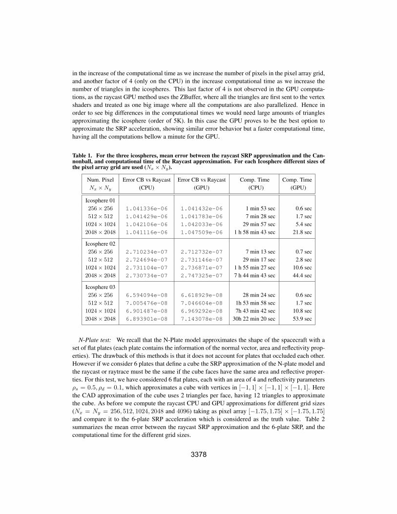
3378
in the increase of the computational time as we increase the number of pixels in the pixel array grid,
and another factor of 4 (only on the CPU) in the increase computational time as we increase the
number of triangles in the icospheres. This last factor of 4 is not observed in the GPU computa-
tions, as the raycast GPU method uses the ZBuffer, where all the triangles are first sent to the vertex
shaders and treated as one big image where all the computations are also parallelized. Hence in
order to see big differences in the computational times we would need large amounts of triangles
approximating the icosphere (order of 5K). In this case the GPU proves to be the best option to
approximate the SRP acceleration, showing similar error behavior but a faster computational time,
having all the computations bellow a minute for the GPU.
Table 1. For the three icospheres, mean error between the raycast SRP approximation and the Can-nonball, and computational time of the Raycast approximation. For each Icosphere different sizes ofthe pixel array grid are used (Nx ×Ny).
Num. Pixel Error CB vs Raycast Error CB vs Raycast Comp. Time Comp. Time
Nx ×Ny (CPU) (GPU) (CPU) (GPU)
Icosphere 01
256× 256 1.041336e-06 1.041432e-06 1 min 53 sec 0.6 sec
512× 512 1.041429e-06 1.041783e-06 7 min 28 sec 1.7 sec
1024× 1024 1.042106e-06 1.042033e-06 29 min 57 sec 5.4 sec
2048× 2048 1.041116e-06 1.047509e-06 1 h 58 min 43 sec 21.8 sec
Icosphere 02
256× 256 2.710234e-07 2.712732e-07 7 min 13 sec 0.7 sec
512× 512 2.724694e-07 2.731146e-07 29 min 17 sec 2.8 sec
1024× 1024 2.731104e-07 2.736871e-07 1 h 55 min 27 sec 10.6 sec
2048× 2048 2.730734e-07 2.747325e-07 7 h 44 min 43 sec 44.4 sec
Icosphere 03
256× 256 6.594094e-08 6.618929e-08 28 min 24 sec 0.6 sec
512× 512 7.005476e-08 7.046604e-08 1h 53 min 58 sec 1.7 sec
1024× 1024 6.901487e-08 6.969292e-08 7h 43 min 42 sec 10.8 sec
2048× 2048 6.893901e-08 7.143078e-08 30h 22 min 20 sec 53.9 sec
N-Plate test: We recall that the N-Plate model approximates the shape of the spacecraft with a
set of flat plates (each plate contains the information of the normal vector, area and reflectivity prop-
erties). The drawback of this methods is that it does not account for plates that occluded each other.
However if we consider 6 plates that define a cube the SRP approximation of the N-plate model and
the raycast or raytrace must be the same if the cube faces have the same area and reflective proper-
ties. For this test, we have considered 6 flat plates, each with an area of 4 and reflectivity parameters
ρs = 0.5, ρd = 0.1, which approximates a cube with vertices in [−1, 1] × [−1, 1] × [−1, 1]. Here
the CAD approximation of the cube uses 2 triangles per face, having 12 triangles to approximate
the cube. As before we compute the raycast CPU and GPU approximations for different grid sizes
(Nx = Ny = 256, 512, 1024, 2048 and 4096) taking as pixel array [−1.75, 1.75] × [−1.75, 1.75]and compare it to the 6-plate SRP acceleration which is considered as the truth value. Table 2
summarizes the mean error between the raycast SRP approximation and the 6-plate SRP, and the
computational time for the different grid sizes.

3379
As we can see in Table 2, the computational time increases as the size of the pixel array grid
increases. Again, we observe a better performance for the GPU methods, and a factor 4 in the
increases of the computational time in all cases, which corresponds to the increases in the number
of pixels casted in each case. However, these results show that the CPU computations give better
approximations than the GPU computations, specially if we are looking for errors bellow 10−8
which is the accuracy limit on the GPU. We note that all the mathematical operations in the GPU
are done using floats while the CPU uses doubles, allowing for better precision. As we can see in
the third column of Table 2, the error starts to increase as we reduce the pixel size as we are reaching
the machine accuracy and the numerical errors affect the final result. This shows that despite having
a faster performance, depending on the desired accuracy the CPU approximation might be the best
option.
Table 2. For the cube, mean error between the raycast SRP approximation and the 6-plate, andcomputational time of the Raycast approximation. For different sizes of the pixel array grid are used(Nx ×Ny).
Num. Pixels Error NP vs Raycast Error NP vs Raycast Comp. Time Comp. Time
Nx ×Ny (CPU) (GPU) (CPU) (GPU)
256× 256 2.622924e-08 2.961771e-08 16.2 sec 0.7 sec
512× 512 1.831568e-08 2.767734e-08 1 min 3 sec 1.8 sec
1024× 1024 1.435540e-08 4.579024e-08 4 min 10 sec 5.5 sec
2048× 2048 7.640938e-09 2.802609e-07 16 min 55 sec 22.4 sec
4096× 4096 2.934854e-09 9.091753e-07 1h 7 min 22 sec 3 min 2 sec
Raycast and Raytrace test: One way to validate the raycast technique is to compare the results
given by two different implementations: the raycast CPU method and the ZBuffer which use the
GPU. Both algorithms are implemented in different ways but should produce the same results
despite small numerical errors. The same comparison can be done between the raytrace single-
scattering (SS) and multiple-scattering (MS) with specular reflection, using the CPU and GPU
versions. We have compared the SRP approximations obtained using these different methods for
the cube used in the previous analyses, however here we only consider the results using a grid of
512× 512 but similar results are observed for different gird sizes.
Table 3 summarizes the results when we compare the CPU with the GPU approximations for
the same method. As we can see the difference between the two SRP approximations for each of
the cases is of the order 10−8 which corresponds to the machine accuracy in the GPU. Table 4, on
the other hand, compares the approximations given by the raycast, raytrace single-scattering and
raytrace multiple-scattering, which must be identical given that the solar rays that bounce off the
cube surface do not intersect the cube again. As we can see in the CPU all the differences are zero,
while in the GPU the Raycast vs Raytrace differences are small but not zero given that the way the
computations are done for each methods are slightly different.
Performance and Accuracy Test
Finally, in order to compare the performance and accuracy of the different methods we have
considered the same spacecraft, and used the different methods to compute the SRP acceleration for
set of azimuth and elevations. The spacecraft used for this is a classical Box-Wing spacecraft that
consists of one cube representing the bus and two flat plates representing the solar panels, where

3380
Table 3. Error between the CPU and GPU computations using raycast and raytrace on a cube andpixel array grid size 512× 512.
Methods Error GPU vs CPU Comp. Time CPU Comp. Time GPU
Raycast (cube) 1.705769e-08 1 min 3 sec 1.8 sec
Raytrace SS (cube) 1.670238e-08 1 min 19 sec 1.9 sec
Raytrace MS (cube) 1.670238e-08 1 min 18 sec 2.3 sec
Table 4. Error between the raycast, raytrace single-scattering (SS) and raytrace multiple-scattering(MS) in both the CPU and GPU, for a cube and a pixel array grid 512× 512.
Comparison CPU GPU
Raycast vs Raytrace SS (cube) 0.00 4.369067e-11
Raycast vs Raytrace MS (cube) 0.00 4.430630e-10
Raytrace SS vs Raytrace MS (cube) 0.00 0.00
each component has different reflectivity properties.3 To compare between CPU and GPU methods,
the size of the pixel array is set to 8.122× 8.122, to ensure it contains the spacecraft for all possible
orientations, and grids of 512×512 and 1024×1024 have been considered for all the finite element
methods. Just as a reference, as all the units are in meters, the size of the pixels for each grid is
0.25mm and 0.062mm, respectively.
To compare the accuracy of the different methods, we need to have the true SRP acceleration,
which in this case we consider as truth the results given by the CPU raytrace multiple-scattering
method with 4 secondary and 16 diffuse rays and a 2048×2048 grid on the pixel array, correspond-
ing to a pixel size of 0.016mm (which took 14h 31min 22sec to compute). We note that we have
taken the CPU approximation as truth in front of the GPU, not because of the performance, but
because as we have seen before the GPU version has a small loss of precision during the transfer of
data in the communications between the CPU and the GPU.
The comparative results between the different finite element methods can be seen in Table 5.
For each method we have computed the SRP acceleration for a set of 162 azimuth and elevations,
using a step size of 20. As in all the analyses performed the execution time is calculated as well
as the mean error between the SRP accelerations and the ground truth. For comparison, we have
also computed the SRP acceleration using the cannonball method (Cr = 1.25, A = 55.7) and an
8-plate approximation of the Box-Wing spacecraft, where each plate has the same area, orientation
and reflective properties as the different faces of the spacecraft.
Notice that cannonball and N-Plate methods are very fast methods as they are very simple to
implement, taking less that one millisecond to evaluate 162 different attitudes. However, the errors
on the SRP approximations are larger compared to the other methods.
The main difference between the CPU and the GPU methods is their performance, the CPU meth-
ods are drastically more computationally demanding as they do not parallelize their computations.
However, as Table 5 shows, there is a very small loss in accuracy in the GPU methods, nothing
significant. For instance, the raycast and raytrace single-scattering errors are almost the same for
both grid sizes. The difference in accuracy between the GPU and CPU approximations is only ob-
served in the raytrace with multiple-scattering, having a factor 2 difference between the results with

3381
Table 5. Comparison table for the different SRP methods.
Method Compt. Time Mean Error Compt. Time Mean Error
Cannonball (CPU) < 1 ms 2.475358e-04
N-plate (CPU) < 1 ms 5.932887e-06
grid size = 512× 512 grid size = 1024× 1024
C Raycast 3 min 20 sec 4.970972e-07 13 min 19 sec 4.510567e-07
P Raytrace SS 3 min 47 sec 1.218539e-07 14 min 51 sec 8.326502e-08
U Raytrace MS 5 min 59 sec 6.786128e-08 24 min 1 sec 2.604322e-08
G Raycast / ZBuffer 1.9 sec 4.905286e-07 9.3 sec 4.484625e-07
P Raytrace SS 2.9 sec 1.025036e-07 10.9 sec 8.059171e-08
U Raytrace MS 3.6 sec 8.675978e-08 12.2 sec 5.891995e-08
1024 × 1024 grid (mean error of 2.6 × 10⁻⁸ for the CPU vs 5.8 × 10⁻⁸ for the GPU). Notice that
these corresponds to errors of order 10−8 close to the GPU accuracy.
Further validity tests should be performed comparing the SRP approximations of our methods
with other validated software like SPAD, or with the SRP accelerations computed for spacecrafts
that are in orbit like LRO. These type of comparisons will be performed in the near future.
CONCLUSION
This paper presents a framework that allows the user to compute high-fidelity approximations of
SRP accelerations for a general spacecraft using raytracing tools. The framework has been designed
to be versatile and easy to use. The framework also allows the user to compute and compare the
SRP accelerations using different methods, like the cannonball, N-plate and finite elements repre-
sentations using raycasting and raytracing, each with different levels of fidelity.
The different finite element methods have been implemented using the CPU and GPU in order
to validate and compare the performance of the different methods. Drastic improvements in the
performance are observed when using the GPU with a negligible loss in the accuracy.
These methods have been validated with simple cases where the SRP accelerations are well
known. Further analyses should be performed in order to validate these methods using real mis-
sion data, which will be performed in the near future.
ACKNOWLEDGMENT
The research by Ariadna Farres has been funded by through Roman Space Telescope project
under the Goddard Planetary and Heliophysics Institute Task 595.001 in collaboration with the
University of Maryland Baltimore County (UMBC) under NNG11PL02A. The research by Anna
Puig is supported under the project 2017-SGR-341.

3382
REFERENCES[1] M. Ziebart, “Generalized Analytical Solar Radiation Pressure Modeling Algorithm for Spacecraft of
Complex Shape,” Journal of Spacecraft and Rockets, Vol. 41, No. 5, 2004.
[2] J. McMahon and D. Scheeres, “New Solar Radiation Pressure Force Model for Navigation,” Journal ofGuidance, Control and Dynamics, Vol. 33, No. 5, 2010.
[3] C. Rodriguez-Solano, U. Hugentobler, and P. Steigenberger, “Adjustable box-wing model for solar radi-ation pressure impacting GPS satellites,” Advances in Space Research, Vol. 49, No. 7, 2012, pp. 1113–1128, 10.1016/j.asr.2012.01.016.
[4] A. Farres, D. Folta, and C. Webster, “Using Spherical Harmonics to model Solar Radiation PressureAccelerations,” 2017 AAS/AIAA Astrodynamics Specialist Conference, August 2017.
[5] P. W. Kenneally and H. Schaub, “Fast spacecraft solar radiation pressure modeling by ray tracingon graphics processing unit,” Advances in Space Research, Vol. 65, April 2020, pp. 1951–1964,10.1016/j.asr.2019.12.028.
[6] S. P. Hughes, R. H. Qureshi, S. D. Cooley, and J. J. Parker, “Verification and Validation of the GeneralMission Analysis Tool (GMAT),” AIAA/AAS Astrodynamics Specialist Conference, August 2014.
[7] A. Milani, A. M. Nobili, and P. Farinella, Non-gravitational perturbations and satellite geodesy. 1987.
[8] D. A. Vallado, Fundamentals of Astrodynamics and Applications. Springer, 1997.
[9] J. T. Kajiya, “The rendering equation,” Proceedings of the 13th annual conference on Computer graph-ics and interactive techniques, 1986, pp. 143–150.
[10] T. Whitted, “An improved illumination model for shaded display,” Proceedings of the 6th annual con-ference on Computer graphics and interactive techniques, 1979, p. 14.
[11] A. Appel, “Some techniques for shading machine renderings of solids,” Proceedings of the April 30–May 2, 1968, spring joint computer conference, 1968, pp. 37–45.
[12] M. Ziebart, High precision analytical solar radiation pressure modelling for GNSS spacecraft. PhDthesis, University of East London, 2001.
[13] M. Ziebart and P. Dare, “Analytical solar radiation pressure modelling for GLONASS using a pixelarray,” Journal of Geodesy, No. 75, 2001, p. 587–599.
[14] B. Rievers, High precision modelling of thermal perturbations with application to Pioneer 10 andRosetta. PhD thesis, University of Bremen, 2012.
[15] B. Rievers, T. Kato, J. v. d. Ha, and C. Lammerzahl, “Numerical Prediction of Satellite Surface Forceswith Application to Rosetta,” 22nd AAS/AIAA Space Flight Mechanics Meeting, December 2011.
[16] P. W. Kenneally and H. Schaub, “High Geometric Fidelity Modeling of Solar Radiation Pressure UsingGraphics Processing Unit,” AAS/AIAA Spaceflight Mechanics Meeting, Napa Valley, California, Feb.14–18 2016. Paper No. AAS-16-500.
[17] P. W. Kenneally and H. Schaub, “Modeling Solar Radiation Pressure With Self-Shadowing UsingGraphics Processing Unit,” AAS Guidance, Navigation and Control Conference, Breckenridge, CO,Feb. 2–8 2017. Paper AAS 17-127.
[18] V. Shumskiy, “GPU ray tracing–comparative study on ray-triangle intersection algorithms,” Transac-tions on Computational Science XIX, pp. 78–91, Springer, 2013.
[19] M. Christen, “Ray tracing on GPU,” Master’s thesis, Univ. of Applied Sciences Basel (FHBB), Vol. 19,2005.