Embed Size (px)
Citation preview
Seventh International Conference onComputational Fluid Dynamics (ICCFD7),Big Island, Hawaii, July 9-13, 2012
ICCFD7-1002
High-Order CENO Finite-Volume Scheme for Low-SpeedViscous Flows on Three-Dimensional Unstructured Mesh
M.R.J. Charest∗, C.P.T. Groth∗ and P.Q. Gauthier∗∗
Corresponding author: [email protected]
∗ University of Toronto Institute for Aerospace Studies4925 Dufferin Street, Toronto, Ontario, Canada M3H 5T6
∗∗ Energy Engineering & Technology, Rolls-Royce Canada Limited9245 Côte-de-Liesse, Dorval, Québec, Canada H9P 1A5
Abstract: High-order discretization techniques offer the potential to significantly reduce the computa-tional costs necessary to obtain accurate predictions when compared to lower-order methods. However,efficient, universally-applicable, high-order discretizations remain somewhat illusive, especially for morearbitrary unstructured meshes and for incompressible/low-speed flows. A novel, high-order, central es-sentially non-oscillatory (CENO), cell-centered, finite-volume scheme is proposed for the solution of theconservation equations of viscous, incompressible flows on three-dimensional unstructured meshes. Theproposed scheme is applied to the pseudo-compressibility formulation of the steady and unsteady Navier-Stokes equations and the resulting discretized equations are solved with a parallel implicit Newton-Krylovalgorithm. For unsteady flows, the temporal derivatives are discretized using the family of high-order back-ward difference formulas (BDF) and the resulting equations are solved via a dual-time stepping approach.The proposed finite-volume scheme for fully unstructured mesh is demonstrated to provide both fast andaccurate solutions for steady and unsteady viscous flows.
Keywords: Numerical Algorithms, Computational Fluid Dynamics, High-Order Methods, IncompressibleFlows.
1 IntroductionComputational fluid dynamics (CFD) has proven to be an important enabling technology in many areas of science andengineering. In spite of the relative maturity and widespread success of CFD in aerospace engineering, there is a varietyof physically-complex flows which are still not well understood and are very challenging to predict by numericalmethods. Such flows include, but are not limited to, multiphase, turbulent, and combusting flows encountered inpropulsion systems (e.g., gas turbine engines and solid propellant rocket motors). These flows present numericalchallenges as they generally involve a wide range of complicated physical/chemical phenomena and scales.
Many flows of engineering interest are incompressible or can be approximated as incompressible to a good degreeof accuracy, i.e. low-speed flows. Incompressible flows can prove challenging to solve numerically because the partialderivative of density with respect to time vanishes. As a result, the governing equations are ill-conditioned. Vari-ous methods for solving the incompressible Navier-Stokes equations have been successfully developed to overcomethis ill-conditioning [1, 2]. These include but are not limited to the pressure-Poisson [3, 4], fractional-step [5, 6],vorticity-based [7, 8], and pseudo-compressibility methods [9]. The equations governing fully-compressible flowshave also been successfully applied to incompressible and low-speed flows using preconditioning techniques [10–15].The pseudo-compressible formulation [9, 16–23] is attractive because it is easily extended to three dimensions and ap-plied in conjunction with high-order schemes. This method was originally referred to as the artificial compressibilitymethod by Chorin [9] but Chang and Kwak [24] introduced the possibly more accurate name “pseudo-compressibility
1
method”.High-order methods have the potential to significantly reduce the cost of modelling physically-complex flows, but
this potential is challenging to fully realize. As such, the development of robust and accurate high-order methods re-mains an active area of research. Standard lower-order methods (i.e, methods up to second order) can exhibit excessivenumerical dissipation for multi-dimensional problems and are often not practical for physically-complex flows. High-order methods offer improved numerical efficiency for accurate solution representations since fewer computationalcells are required to achieve a desired level of accuracy [25]. For hyperbolic conservation laws and/or compressibleflow simulations, the main challenge involves obtaining accurate discretizations while ensuring that discontinuities andshocks are handled reliably and robustly [26]. High-order schemes for elliptic partial differential equations (PDEs) thatgovern diffusion processes should satisfy a maximum principle, even on stretched/distorted meshes, while remainingaccurate [27]. There are many studies of high-order schemes developed for finite-volume [26, 28–37], discontinuousGalerkin [38–42], and spectral finite-difference/finite-volume methods [43–47] on both structured and unstructuredmesh. In spite of many advances, there is still no consensus for a robust, efficient, and accurate scheme that fully dealswith all of the aforementioned issues and is universally applicable to arbitrary meshes.
Harten et al. [26] originally proposed the essentially non-oscillatory (ENO) high-order finite-volume scheme whichachieves monotonicity by avoiding the use of computational stencils that contain discontinuities. Weighted ENO(WENO) schemes attempt to simplify the ENO procedure by adopting a stencil-weighting approach [32, 34, 35].However, both the ENO and WENO schemes encounter difficulties when selecting appropriate stencils on generalmulti-dimensional unstructured meshes [29, 30, 33, 48] and using these stencils can produce poor conditioning of thelinear systems involved in performing the solution reconstruction [33, 48]. These difficulties, along with the associatedcomputational cost and complexities of the ENO and WENO finite-volume schemes, have somewhat limited theapplicable range of ENO and WENO.
Ivan and Groth [49, 50] proposed a high-order Central Essentially Non Oscillatory (CENO), cell-centered, finite-volume scheme that was demonstrated to remain both accurate and robust in a variety of physically-complex flows.The CENO scheme is based on a hybrid solution reconstruction procedure that combines an unlimited high-orderk-exact, least-squares reconstruction technique with a monotonicity preserving limited piecewise linear least-squaresreconstruction algorithm. Fixed central stencils are used for both the unlimited high-order k-exact reconstruction andthe limited piecewise linear reconstruction. Switching between the two reconstruction algorithms is determined by asolution smoothness indicator that indicates whether or not the solution is resolved on the computational mesh. Thishybrid approach avoids the complexities associated with reconstruction on multiple stencils that other essentially non-oscillatory (ENO) and weighted ENO schemes can encounter. Originally developed for structured two-dimensionalmesh, this scheme has been successfully extended to two- and three-dimensional unstructured mesh by McDonaldet al. [51].
The application of high-order solution methods to the pseudo-compressibility approach is not new. Rogers andKwak [21, 52] and Qian and Zhang [23] employed high-order finite-difference discretizations up to fifth- and sixth-order accuracy, respectively. Using a finite-volume discretization, Chen et al. [53] applied a fifth-order WENO schemeon two-dimensional structured mesh. However, these discretizations are not easily applied to three-dimensional un-structured mesh.
Implicit solution algorithms are commonly applied to improve the stability and convergence of pseudo-com-pressibility approaches. Implicit algorithms that have been applied to the pseudo-compressible formulation of theNavier-Stokes equations include: approximate factorization [19, 54], LU-SGS/SSOR algorithms [23, 53, 55] andline-relaxation techniques [22, 52]. Due to various approximations and/or linearizations, these schemes are not fully-implicit and their application to unstructured mesh is not straightforward. Jacobian-free Newton-Krylov methods [56–59] offer significant improvements over these types of implicit schemes in terms of rapid convergence. They canrobustly handle stiff-wave systems, strong non-linear couplings between equations and offer the potential of quadraticconvergence [59, 60].
All of the applications of the pseudo-compressibility formulation discussed previously have focused on constantdensity flows. They are not directly applicable to more general low-speed flows that involve combustion or multiplefluids/species. Several researchers have applied the standard pseudo-compressibility approach in conjunction withinterface-capturing methods to track the discontinuities in density encountered in multi-fluid flows [61, 62]. There areother approaches that are more applicable to the combusting flows encountered in propulsion systems. For example,Riedel [63] applied the pseudo-compressibility approach to reacting flows using an artificial-dissipation-based finite-volume method. A characteristic-based scheme using the pseudo-compressibility approach was derived by Shapiro andDrikakis [64] which is applicable for variable-density, multi-species, isothermal flows. A similar characteristic-based
2
scheme for constant density flows with heat transfer was developed by Azhdarzadeh and Razavi [65].In this paper, the high-order CENO finite-volume scheme is extended to solve the equations governing incom-
pressible, viscous, laminar flows with variable density on three-dimensional general unstructured mesh. For steadyflows, the equations are solved using the pseudo-compressibility approach coupled with an implicit Newton-Krylovalgorithm. The proposed scheme is extended to unsteady flows via a dual-time stepping approach. The resultingalgorithm is applied to both steady and unsteady flows and analyzed in terms of accuracy, computational cost, andparallel performance. In particular, the spatial and temporal accuracy of solutions are examined and the influence ofmesh resolution on accuracy is assessed for several idealized flow problems. Both the steady flow over an isothermalflat plate and the unsteady decay of Taylor vortices are studied here.
2 Pseudo-Compressibility Approach for Variable Density Low Speed FlowsIn the present research, the equations governing viscous, laminar, compressible flows at low Mach numbers are con-sidered. In three space dimensions, the governing partial-differential equations are
∂ρ
∂t+ ∇ · (ρ~v) = 0 (1a)
∂
∂t(ρ~v) + ∇ · (ρ~v~v + p~I) = ∇ · ~τ (1b)
∂
∂t(ρh) + ∇ ·
(ρ~vh
)= ∇ · ~q (1c)
where t is the time, p is the total pressure, ρ is the fluid density, ~v is the bulk fluid velocity vector, h =∫ T
T0cp dT is the
fluid enthalpy, cp is the fluid specific heat, T is the temperature, ~q = −λ∇T is the heat flux vector, and λ is the fluidthermal conductivity. The fluid stress tensor is given by
τi j = µ
[(∂ui
∂x j+∂u j
∂xi
)−
23δi j∂uk
∂xk
](2)
where µ is the dynamic viscosity. At low speeds, density becomes weakly coupled to pressure via the ideal gas law.Here, we assume that pressure is constant and density is a function of temperature only, ρ = ρ(T ).
For low-Mach-number and incompressible flows, the pseudo-compressibility method modifies the partial deriva-tives of density with respect to time [9, 16, 18, 66]. In the original formulation of Chorin [9] for incompressible flows,a pressure time derivative was added to the steady form of the continuity equation and the primitive form of the gov-erning equations were solved using a time-marching procedure. Turkel [18] derived the conservative form of Chorin’smodified governing equations and showed that time derivatives of pressure should also be added to the momentumequations. Applying the pseudo-compressibility approach to Eq. (1), the resulting governing equations are
1β
∂p∂τ
+ ∇ · (ρ~v) = 0 (3a)
ρ∂~v∂τ
+α~vβ
∂p∂τ
+ ∇ · (ρ~v~v + p~I) = ∇ · ~τ (3b)
ρ∂h∂τ
+αhβ
∂p∂τ
+ ∇ ·(ρ~vh
)= ∇ · ~q (3c)
where β is the pseudo-compressibility factor, α is a preconditioning parameter, and τ denotes the pseudo-time sincethe modified equations are no longer time-accurate. The preconditioning parameter, α, controls how the originalgoverning equations are modified. The original pseudo-compressibility method of Chorin [9] corresponds to α = 0.When α = 1 or 2, the pressure time derivatives are added directly to the conserved or primitive formulation of thegoverning equations, respectively.
Time-accuracy is regained using a dual-time-stepping approach [21, 22, 67–69]. The time-accurate form of Eq. (3)is
∂U∂t
+ Γ∂W∂τ
+∂
∂x(E − Ev) +
∂
∂y(F − Fv) +
∂
∂z(G −Gv) = 0 (4)
3
where U and W are the vectors of conserved and primitive variables, ~F = [E,F,G] and ~Fv = [Ev,Fv,Gv] are theinviscid and viscous solution flux dyads, and Γ is the transformation matrix. They are defined as
U =
ρρuρvρwρh
, W =
puvwT
, E =
ρu
ρu2 + pρuvρuwρuh
, F =
ρvρvu
ρv2 + pρvwρvh
, G =
ρwρwuρwv
ρw2 + pρvh
,
Ev =
0τxx
τxy
τxz
λ∂T∂z
, Fv =
0τyx
τyy
τyz
λ∂T∂z
, Gv =
0τzx
τyz
τzz
λ∂T∂z
,Γ =
1β
0 0 0 0
α
βu ρ 0 0 0
α
βv 0 ρ 0 0
α
βw 0 0 ρ 0
α
βh 0 0 0 ρcp
.
2.1 EigenstructureBased on the analysis conducted by Turkel [18] and the numerical results obtained by Qian et al. [70] and Lee and Lee[71], the optimal value of α is 2. However, Malan et al. [72, 73] and Lee and Lee [71] found that a loss of robustnesscan occur for α > 1 if β is too small. This loss of robustness occurs because the determinant of the modal matrix canbe zero when α > 1. Since larger values of α display better convergence characteristics [70, 71], α = 1 was selectedfor the current work. For α = 1, the Jacobian matrix of the inviscid system with respect to the primitive variables is
A = Γ−1∂(~F · n
)∂W
=
0 nxρβ nyρβ nzρβ 0
nx
ρq 0 0 0
ny
ρ0 q 0 0
nz
ρ0 0 q 0
0 0 0 0 q
(5)
where q = ~v · n and c2 = q2 + 4β. The resulting matrix of right eigenvectors is
R =
−ρ
2(q − c) −
ρ
2(q + c) 0 0 0
nx nx −ny −nz 0
ny ny nx 0 0
nz nz 0 nx 0
0 0 0 0 1
(6)
4
Table 1. Gauss quadrature rules used for cell face integration.
Reconstruction Tetrahedra Cartesian / Hexahedra
Points Polynomial Degree Points Polynomial Degree
Constant (k=0) 1 1 1 1Linear (k=1) 1 1 1 1Quadratic (k=2) 3 2 4 3Cubic (k=3) 4 3 4 3Quartic (k=4) 6 4 9 5
The eigenvalues of the inviscid system defined by Eq. (3) in a particular direction are
λ =
12
un −12
√un
2 + 4β
un
un
un
12
un +12
√un
2 + 4β
(7)
where un is the velocity of the bulk flow projected onto the direction vector of interest.
3 CENO Finite-Volume SchemeIn the proposed cell-centered finite-volume approach, the physical domain is discretized into finite-sized computationalcells and the integral forms of conservation laws are applied to each individual cell. For a cell i, the approach resultsin the following coupled system of partial differential equations (PDEs) for cell-averaged solution quantities:
dUi
dt+ Γi
dWi
dτ= −
1Vi
(~F − ~Fv
)· n dA = −Ri (8)
where the overbar denotes cell-averaged quantities, Vi is the cell volume, A is the area of the face and n is the unitvector normal to a given face. Applying Gauss quadrature to evaluate the surface integral in Eq. (8) produces a set ofnonlinear ordinary differential equations (ODEs) given by
dUi
dt+ Γi
dWi
dτ= −
1Vi
Nf∑l=1
NG∑m=1
[ω
(~F − ~Fv
)· nA
]i,l,m
(9)
where Nf is the number of faces (equal to 4 for tetrahedra and 6 for hexahedra), NG is the number of quadrature pointsand ω is the corresponding quadrature weight. In Eq. (9), the number of quadrature points required along each faceis a function of the reconstruction order and number of spatial dimensions. For tetrahedra and Cartesian (hexahedrawith rectangular faces) cells, Gauss quadrature points can be directly mapped from the canonical form to the Cartesiancoordinate system. More general hexahedra can have non-rectangular faces or faces composed of vertices that do notall lie on a particular plane. In this case, the Gauss quadrature points are mapped to the Cartesian coordinate systemusing a trilinear coordinate transformation [74, 75]. The coefficients for the quadrature rules applied here are tabulatedby Felippa [76] and summarized in Table 1.
3.1 CENO ReconstructionEvaluating Eq. (9) requires integration of the numerical flux along the cell faces, but only cell-averaged quantitiesare known. The high-order CENO method uses a hybrid solution reconstruction process to interpolate the primitivesolution state at the Gauss quadrature points along each face [49, 50]. This hybrid approach involves a fixed central
5
stencil in smooth or fully-resolved regions which is switched to a limited piecewise linear reconstruction when dis-continuities in solution content are encountered. This switching provides a means of eliminating spurious oscillationsthat can occur near regions where the solution is under-resolved. It is facilitated by a parameter called the smoothnessindicator which indicates the current level of resolution.
Even though most features of low-speed flows are relatively smooth, there are cases where discontinuities canoccur, such as across flame fronts or fluid interfaces. Oscillations can even occur for relatively smooth flows whenthere is insufficient mesh resolution.
3.1.1 k-Exact Reconstruction
The CENO spatial discretization scheme is based on the high-order k-exact least-squares reconstruction technique ofBarth [28]. The k-exact higher-order reconstruction algorithm begins by assuming that the solution within each cellcan be represented by the following Taylor series expansion in three dimensions:
uki (x, y, z) =
(p1+p2+p3)≤k∑p1=0
∑p2=0
∑p3=0
(x − xi)p1 (y − yi)p2 (z − zi)p3 Dp1 p2 p3 (10)
where uki is the reconstructed solution quantity, (xi,yi,zi) are the coordinates of the cell centroid, k is the order of
the piecewise polynomial interpolant and Dp1 p2 p3 are the unknown coefficients of the Taylor series expansion. Thesummation indices, p1, p2 and p3, must always satisfy the condition that (p1 + p2 + p3) ≤ k.
The following conditions are applied to determine the unknown coefficients: i) the solution reconstruction mustreproduce polynomials of degree N ≤ k exactly; ii) the mean or average value within the computational cell must bepreserved; and iii) the reconstruction must have compact support. The second condition states that
ui =1Vi
$Vi
uki (x, y, z) dV (11)
where ui is the cell average.The third condition dictates the number and location of neighboring cells included in the reconstruction. For a
compact stencil, the minimum number of neighbors is equal to the number of unknowns minus one (because of theconstraint imposed by Eq. (11)). For any type of mesh, the total number of unknown coefficients for a particular orderis given by
N =1d!
d∏n=1
(k + n) (12)
where d represents the number of space dimensions. In three-dimensions, there are four, ten, twenty and thirty-fiveunknown coefficients for k=1, k=2, k=3 and k=4, respectively. Additional neighbors are included to ensure that thestencil is not biased in any particular direction and that the reconstruction remains reliable on poor quality mesheswith high aspect ratio cells [49]. For each neighboring cell, p, a constraint is formed by requiring that
up =1
Vp
$Vp
uki (x, y, z) dV (13)
Since the constraints of Eqs. (11) and (13) result in an over-determined system of linear equations, a least-squaressolution for the coefficients, Dp1 p2 p3 , is obtained in each cell. Equation (11) is strictly enforced by Gaussian eliminationand a minimum-error solution to the remaining constraint equations is sought. The resulting coefficient matrix of thelinear system depends only on the mesh geometry and can be partially calculated and stored prior to computations [36,77]. Either a Householder QR factorization algorithm or orthogonal decomposition by the SVD method was usedto solve the weighted least-squares problem [78]. Weighting is applied here to each control volume to improve thelocality of the reconstruction [79]. An inverse distance weighting formula is applied. For the reconstruction in cell i,
w j =1
|~x j − ~xi|, (14)
where ~x j is the centroid of the neighbor cell j.
6
3.1.2 Reconstruction at Boundaries
To enforce conditions at physical boundaries, the least-squares reconstruction was constrained in adjacent controlvolumes without altering the reconstruction order of accuracy [36, 50]. Constraints are placed on the least-squaresreconstruction for each variable to obtain the desired value/gradient (Dirichlet/Neumann) at each Gauss integrationpoint. Here we implement them as Robin boundary conditions
f(~x)
= a(~x)
fD(~x)
+ b(~x)
fN(~x)
(15)
where a(~x)
and b(~x)
define the contribution of the Dirichlet, fD(~x), and Neumann, fN
(~x), components, respectively.
In terms of the cell reconstruction, the Dirichlet condition is simply expressed as
fD(~xg
)= uk
(~xg
)(16)
where ~xg is the location of the Gauss quadrature point. The Neumann condition is
fN(~xg
)= ∇uk
(~xg
)· ng =
(p1+p2+p3)≤k∑∑∑p1+p2+p3=1
∆xp1−1∆yp2−1∆zp3−1[p1∆y∆znx + p2∆x∆yny + p3∆x∆ynz
]Dp1 p2 p3 (17)
where ∆(·) = (·)g − (·)i, the subscript i denotes the location of the centroid of the cell adjacent to the boundary and gdenotes the Gauss quadrature point.
Exact solutions to the boundary constraints, Eq. (15), are sought. This adds linear equality constraints to theoriginal least-squares problem described in Section 3.1.1. Gaussian elimination with full pivoting is first appliedto remove the additional boundary constraints and the remaining least-squares problem is solved as described inSection 3.1.1.
For inflow/outflow or farfield-type boundary conditions where the reconstructed variables are not related, the con-straints may be applied separately to each variable. More complex boundary conditions involving linear combinationsof solution variables, such as symmetry or inviscid solid walls (~v · n = 0), can cause the reconstruction coefficients inEq. (10) for different variables to become coupled. For these types of coupled boundary conditions, the reconstructionfor all of the coupled solution variables is performed together [37, 50]. Thus the final matrix A for the constrainedleast-squares reconstruction contains the individual constraints for each variable, the relational constraints, and theapproximate mean conservation equations for each variable.
3.1.3 Smoothness Indicator
After performing a k-exact reconstruction for each solution variable in each computational cell, the smoothness indi-cator is computed for every reconstructed variable to identify under-resolved solution content. It is evaluated as
S =α
max [(1 − α), δ](SOS − DOF)
DOF − 1(18)
where α is a smoothness parameter, δ is a tolerance to avoid division by zero (equal to 10−8), DOF is the number ofdegrees off freedom and SOS is the size of the stencil. The smoothness parameter, α, for a cell i is given by
α = 1 −
∑p
[uk
p(xp, yp, zp) − uki (xp, yp, zp)
]2
∑p
[uk
p(xp, yp, zp) − ui
]2 (19)
where u is the solution variable of interest, the subscript p refers to the cells in the reconstruction stencil, ukp(xp, yp, zp)
is the reconstructed solution in cell p evaluated at the cell’s centroid (xp, yp, zp), uki (xp, yp, zp) is the projected value of
the reconstruction polynomial for cell i evaluated at (xp, yp, zp), and ui is the average value for cell i. By definition,α can have a value between negative infinity and one. A value of unity indicates that the solution is smooth whereassmall or negative values indicate large variations in solution content within the reconstruction stencil.
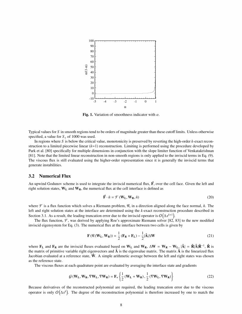
The behavior of the smoothness indicator is demonstrated in Fig. 1. As α approaches unity, the smoothnessindicator grows rapidly. Solutions are deemed smooth when the value of S is above critical value, S c. Previousstudies found that values for S c between 1000–5000 provided an excellent balance between stability and accuracy [49].
7
-10
0
10
20
30
40
50
60
70
80
90
100
-5 -4 -3 -2 -1 0 1
α/(
1-α
)
α
Fig. 1. Variation of smoothness indicator with α.
Typical values for S in smooth regions tend to be orders of magnitude greater than these cutoff limits. Unless otherwisespecified, a value for S c of 1000 was used.
In regions where S is below the critical value, monotonicity is preserved by reverting the high-order k-exact recon-struction to a limited piecewise linear (k=1) reconstruction. Limiting is performed using the procedure developed byPark et al. [80] specifically for multiple dimensions in conjunction with the slope limiter function of Venkatakrishnan[81]. Note that the limited linear reconstruction in non-smooth regions is only applied to the inviscid terms in Eq. (9).The viscous flux is still evaluated using the higher-order representation since it is generally the inviscid terms thatgenerate instabilities.
3.2 Numerical FluxAn upwind Godunov scheme is used to integrate the inviscid numerical flux, ~F, over the cell face. Given the left andright solution states, WL and WR, the numerical flux at the cell interface is defined as
~F · n = F (WL,WR, n) (20)
where F is a flux function which solves a Riemann problem, R, in a direction aligned along the face normal, n. Theleft and right solution states at the interface are determined using the k-exact reconstruction procedure described inSection 3.1. As a result, the leading truncation error due to the inviscid operator is O
(∆xk+1
).
The flux function, F , was derived by applying Roe’s approximate Riemann solver [82, 83] to the new modifiedinviscid eigensystem for Eq. (3). The numerical flux at the interface between two cells is given by
F (R (WL,WR)) =12
(FR + FL) −12|A|∆W (21)
where FL and FR are the inviscid fluxes evaluated based on WL and WR, ∆W = WR −WL, |A| = R|Λ|R−1, R isthe matrix of primitive variable right eigenvectors and Λ is the eigenvalue matrix. The matrix A is the linearized fluxJacobian evaluated at a reference state, W. A simple arithmetic average between the left and right states was chosenas the reference state.
The viscous fluxes at each quadrature point are evaluated by averaging the interface state and gradients
G (WL,WR,∇WL,∇WR) = Fv
{12
(WL + WR) ,12
(∇WL,∇WR)}
(22)
Because derivatives of the reconstructed polynomial are required, the leading truncation error due to the viscousoperator is only O
(∆xk
). The degree of the reconstruction polynomial is therefore increased by one to match the
8
leading truncation error introduced by the inviscid operator. The Gauss quadrature rule is selected to maintain an orderof accuracy of k + 1 when integrating the fluxes over the cell faces.
For piecewise-linear (k = 1) representations, second-order (k +1) accuracy of the viscous operator can be achievedwithout increasing the degree of the polynomial interpolatant. In this case, the average gradient at the interface isevaluated by [84]
∇Wi+1/2 =(Wn −Wp
) nn · ~rp→n
+
(∇W − ∇W · ~rp→n
nn · ~rp→n
)(23)
where ∇W is the weighted average of the cell interface
∇W = α∇Wp + (1 − α)∇Wn (24)α = Vp/(Vp + Vn)
Equation (23) is second-order accurate if the gradient representation is also second-order accurate. Thus, k + 1 recon-struction is not required for k = 1.
3.3 Inexact Newton Method for Steady and Unsteady FlowsIntegration of the governing equations is performed in parallel to fully take advantage of modern computer archi-tectures. This is carried out by dividing the computational domain up using a parallel graph partitioning algorithm,called Parmetis [85], and distributing the computational cells among the available processors. Solutions for each com-putational sub-domain are simultaneously computed on each processor. The proposed computational algorithm wasimplemented using the message passing interface (MPI) library and the Fortran 90 programming language [86]. Ghostcells, which surround an individual local solution domain and overlap cells on neighboring domains, are used to sharesolution content through inter-block communication.
Newton’s method is applied in this work for both steady state relaxation and transient continuation. For transientcalculations, a dual-time-stepping approach is used [21, 22, 67–69] with the family of high-order backwards differenceformulas to discretize the physical time derivative. In both cases, steady and unsteady, Newton’s method is used torelax
R∗(W) = R +dWdt
= 0 (25)
where dWdt = 0 for steady problems.
This particular implementation follows the algorithm developed previously by Groth et al. [87–89] specificallyfor use on large multi-processor parallel clusters. The implementation makes use of a Jacobian-free inexact Newtonmethod coupled with an iterative Krylov subspace linear solver.
3.3.1 Inexact Newton Method For Steady Problems
For steady problems, a solution to Eq. (25) is sought by iteratively solving a sequence of linear systems given an initialestimate, W0. Successively improved estimates are obtained by solving(
∂R∂W
)k
∆Wk = J(Wk)∆Wk = −R(Wk) (26)
where J = ∂R∂W is the residual Jacobian. The improved solution at step k is then determined from
Wk+1 = Wk + ∆Wk (27)
The Newton iterations proceed until some desired reduction of the norm of the residual is achieved and the condition‖R(Wk)‖ < ε‖R(W0)‖ is met. The tolerance, ε, used in this work was typically 10−7 for steady problems.
For a system of nonlinear equations, each step of Newton’s method requires the solution of the linear problemJx = b where x = ∆W and b = −R(W). This system tends to be relatively large, sparse, and non-symmetric for whichiterative methods have proven much more effective than direct methods. One effective method for a large variety ofproblems which is used here is the generalized minimal residual (GMRES) technique of Saad and co-workers [58, 90–92]. This is an Arnoldi-based solution technique which generates orthogonal bases of the Krylov subspace to construct
9
the solution. The technique is particularly attractive because the matrix J is not explicitly formed and instead onlymatrix-vector products are required at each iteration to create new trial vectors. This drastically reduces the requiredstorage. Another advantage is that iterations are terminated based on only a by-product estimate of the residual whichdoes not require explicit construction of the intermediate residual vectors or solutions. Termination also generally onlyrequires solving the linear system to some specified tolerance, ‖Rk + Jk∆Wk‖2 < ζ‖R(Wk)‖2, where ζ is typically inthe range 0.1−0.5 [56]. We use a restarted version of the GMRES algorithm here, GMRES(m), that minimizes storageby restarting every m iterations.
Right preconditioning J is performed to help facilitate the solution of the linear system without affecting thesolution residual, b. The preconditioning takes the form(
JM−1)
(Mx) = b (28)
where M is the preconditioning matrix. A combination of an additive Schwarz global preconditioner and a blockincomplete lower-upper (BILU) local preconditioner is used. In additive Schwarz preconditioning, the solution ineach block is updated simultaneously and shared boundary data is not updated until a full cycle of updates has beenperformed on all domains. The preconditioner is defined as follows
M−1 =
Nb∑k=1
BTk M−1
k Bk (29)
where Nb is the number of blocks and Bk is the gather matrix for the kth domain. The local preconditioner, M−1k , in
Eq. (29) is based on block ILU(p) factorization [92] of the Jacobian for the first order approximation of each domain.The level of fill, p, was maintained at between 0–1 to reduce storage requirements. Larger values of p typically offerimproved convergence characteristics for the linear system at the expense of storage. To further reduce computationalstorage, reverse Cuthill-McKee matrix reordering is used to permute the Jacobian’s sparsity pattern into a band matrixform with a small bandwith [93].
3.3.2 Implicit-Euler Startup
Newton’s method can fail when initial solution estimates fall outside the radius of convergence. To ensure globalconvergence of the algorithm, the implicit Euler startup procedure with successive evolution/relaxation (SER) pro-posed by Mulder and Van Leer [94] was used. Application of this startup procedure to the semi-discrete form of thegoverning equations gives Γ
∆τk +
(∂R∂W
)k ∆Wk = −Rk (30)
where ∆τk is the time step. In the SER approach, the time step is varied from some small finite value and graduallyincreased as the steady state solution is approached. As ∆τk → ∞, Newton’s method is recovered.
In the quasi-Newton and SER methods, the time step size was determined by considering the inviscid Courant-Friedrichs-Lewy (CFL) and viscous Von Neumann stability criteria based on the pseudo-compressible system. Themaximum permissible time step for each local cell is determined by
∆τk ≤ CFL ·min[∆xλ+,ρ∆x2
µ
](31)
where CFL is a constant greater than zero which determines the time step size and ∆x = V1/3 is a measure of the gridsize. Using SER, the CFL number for the kth iteration is computed using the following relation:
CFLk = CFL0 ‖R(W0)‖‖R(Wk)‖
(32)
During the startup phase of the Newton calculation, a value for CFL between 10–100 is typically used. The minimumvalue of β was chosen based on the following formulation proposed by Turkel [18]:
β = max[2(u2 + v2 + w2
), ε
](33)
where ε is a smallness parameter.
10
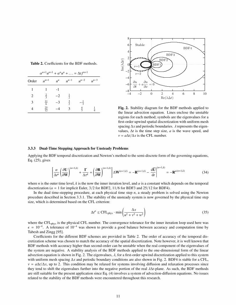
Table 2. Coefficients for the BDF methods.
αn+1un+1 + αnun + . . . = ∆t f n+1
Order un+1 un un−1 un−2 un−3
1 1 -1
2 23 −2 1
2
3 116 −3 3
2 − 13
4 2512 −4 3 4
314
−4 −2 0 2 4 6 8 10−8
−6
−4
−2
0
2
4
6
8
Re(λ∆t)
Im(λ∆t)
BDF1
BDF2
BDF3
BDF4
ν=2
ν=1
Stable
∂u
∂t+ a
∂u
∂x= 0
Fig. 2. Stability diagram for the BDF methods applied tothe linear advection equation. Lines enclose the unstableregions for each method; symbols are the eigenvalues for afirst-order upwind spatial discretization with uniform meshspacing ∆x and periodic boundaries. λ represents the eigen-values, ∆t is the time step size, a is the wave speed, andν = a∆t/∆x is the CFL number.
3.3.3 Dual-Time Stepping Approach for Unsteady Problems
Applying the BDF temporal discretization and Newton’s method to the semi-discrete form of the governing equations,Eq. (25), gives α∆tn
(∂U∂W
)(n+1,k)
+Γ
∆τk +
(∂R∂W
)(n+1,k) ∆W(n+1,k) = −R(n+1,k) −dUdt
∣∣∣∣∣∣(n+1,k)
= −R∗(n+1,k) (34)
where n is the outer time level, k is the now the inner iteration level, and α is a constant which depends on the temporaldiscretization (α = 1 for implicit Euler, 3/2 for BDF2, 11/6 for BDF3 and 25/12 for BDF4).
In the dual time-stepping procedure, at each physical time step n, a steady problem is solved using the Newtonprocedure described in Section 3.3.1. The stability of the unsteady system is now governed by the physical time stepsize, which is determined based on the CFL criterion:
∆tn ≤ CFLphys ·min(
∆xu2 + v2 + w2
)(35)
where the CFLphys is the physical CFL number. The convergence tolerance for the inner iteration loop used here wasε = 10−4. A tolerance of 10−4 was shown to provide a good balance between accuracy and computation time byTabesh and Zingg [95].
Coefficients for the different BDF schemes are provided in Table 2. The order of accuracy of the temporal dis-cretization scheme was chosen to match the accuracy of the spatial discretization. Note however, it is well known thatBDF methods with accuracy higher than second-order can be unstable when the real component of the eigenvalues ofthe system are negative. A stability analysis of the BDF methods applied to the one-dimensional form of the linearadvection equation is shown in Fig. 2. The eigenvalues, λ, for a first-order upwind discretization applied to this systemwith uniform mesh spacing ∆x and periodic boundary conditions are also shown in Fig. 2. BDF4 is stable for a CFL,ν = a∆t/∆x, up to 2. This condition may be relaxed for systems involving diffusion and relaxation processes sincethey tend to shift the eigenvalues further into the negative portion of the real λ∆t-plane. As such, the BDF methodsare still suitable for the present application since Eq. (4) involves a system of advection-diffusion equations. No issuesrelated to the stability of the BDF methods were encountered throughout this research.
11
4 Results For Three-Dimensional Unstructured MeshThe proposed finite-volume scheme was assessed in terms of accuracy, stability, and computational efficiency. Numer-ical results for both smooth and discontinuous function reconstructions as well as solutions for steady and unsteadyviscous flows on three-dimensional unstructured mesh were obtained. All computations were performed on a highperformance parallel cluster consisting of 3,780 Intel Xeon E5540 (2.53GHz) nodes with 16GB RAM per node. Thecluster is connected with a high speed InfiniBand switched fabric communications link.
An error analysis is performed whenever exact solutions are present. Accuracy is assessed based on the L1 and L2norms of the error between the exact solution and the numerical solution. The Lp norm of the error is evaluated overall cells, i,
Lp = ‖Error‖p =
1VT
∑i
$Vi
∣∣∣uki (x, y, z) − uexact(x, y, z)
∣∣∣p dV
1/p
(36)
where VT is the total volume of the domain and uexact(x, y, z) is the exact solution. This integration is performedusing an adaptive cubature algorithm developed by Cools et al. [96, 97] for integrating functions over a collection ofN-dimensional hyperrectangles and simplices.
4.1 Spherical Cosine FunctionThe first case considered is the reconstruction of a smooth spherical cosine function. The function, which is smooth inall directions, is described by
u(r) = 1 +13
cos(r) (37)
where r = 10√
x2 + y2 + z2 is the radial position. The solution is computed on a unit cube using grids composedof tetrahedral, Cartesian, and irregular hexahedral cells with varying levels of resolution. The irregular hexahedralmeshes were generated by randomly perturbing the internal nodes of an initial Cartesian mesh.
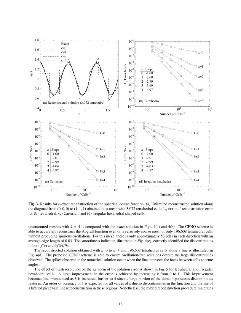
The results for the unlimited k-exact reconstruction of the three-dimensional spherical cosine function performedon a coarse mesh with 3,072 tetrahedral elements is illustrated in Fig. 3(a). As the order of the piecewise polynomialinterpolant is increased from k=0 to k=3, the reconstructed solution rapidly approaches the exact solution. There isalmost no visible difference between the exact solution and the reconstructed solution for k=4 (not shown in figure).
An analysis of the L2 norm of the error in the numerical solution as the tetrahedral mesh resolution is increased,illustrated in Fig. 3(b) for various values of k, confirms that k-exact reconstruction of a smooth function yields anorder of accuracy equal to k+1. Similar results for the error analysis are observed for meshes composed of Cartesian,Fig. 3(c), and irregular hexahedrals, Fig. 3(d).
4.2 Abgrall’s FunctionThe Abgrall function [29] possesses a number of solution discontinuities which test a high-order spatial discretization’sability to maintain monotonicity. Reconstructions of this function using the proposed high-order CENO algorithm forunstructured meshes are obtained to ensure the effectiveness of the smoothness indicator defined in Eq. (18). Eventhough the performance of this formulation for S was already verified using the Abgrall function and structuredmesh [49], it has not been fully evaluated for unstructured mesh. McDonald et al. [51] only obtained preliminaryresults for this function on tetrahedral meshes. The Abgrall function is defined as
u(x, y) =
{f (x − cot
√π/2 y) if x ≤ cos(πy)/2, and
f (x + cot√π/2 y) + cos(2πy) if x > cos(πy)/2.
(38)
where
f (r) =
−r sin
(3πr2/2
)if r ≤ −1/3,
| sin(2πr)| if |r| < 1/3, and2r − 1 + sin(3πr)/6 if r ≥ 1/3.
(39)
and r =√
x2 + y2. Here, it is applied in three dimensions to a cube with length 2 by extruding the two-dimensionalfunction along the z axis. The reconstructed solution obtained using the proposed high-order CENO algorithm for
12
r
u(r
)
0 0.5 1 1.50.4
0.6
0.8
1
1.2
1.4
1.6
1.8Exact
k=0
k=1
k=2
k=3
(a) Reconstructed solution (3,072 tetrahedra)
Number of Cells1/3
L2 E
rror
Norm
101
102
103
1010
109
108
107
106
105
104
103
102
101
k Slope
0 1.00
1 2.00
2 2.99
3 3.99
4 4.97
k=0
k=1
k=2
k=3
k=4(b) Tetrahedra
Number of Cells1/3
L2 E
rror
Norm
101
102
103
1010
109
108
107
106
105
104
103
102
101
k Slope
0 1.00
1 2.01
2 2.99
3 4.04
4 4.97
k=0
k=1
k=2
k=3
k=4(c) Cartesian
Number of Cells1/3
L2 E
rror
Norm
101
102
103
1010
109
108
107
106
105
104
103
102
101
k Slope
0 1.00
1 2.01
2 2.99
3 4.03
4 4.97
k=0
k=1
k=2
k=3
k=4(d) Irregular hexahedra
Fig. 3. Results for k-exact reconstruction of the spherical cosine function. (a) Unlimited reconstructed solution alongthe diagonal from (0, 0, 0) to (1, 1, 1) obtained on a mesh with 3,072 tetrahedral cells; L2 norm of reconstruction errorfor (b) tetrahedral, (c) Cartesian, and (d) irregular hexahedral shaped cells.
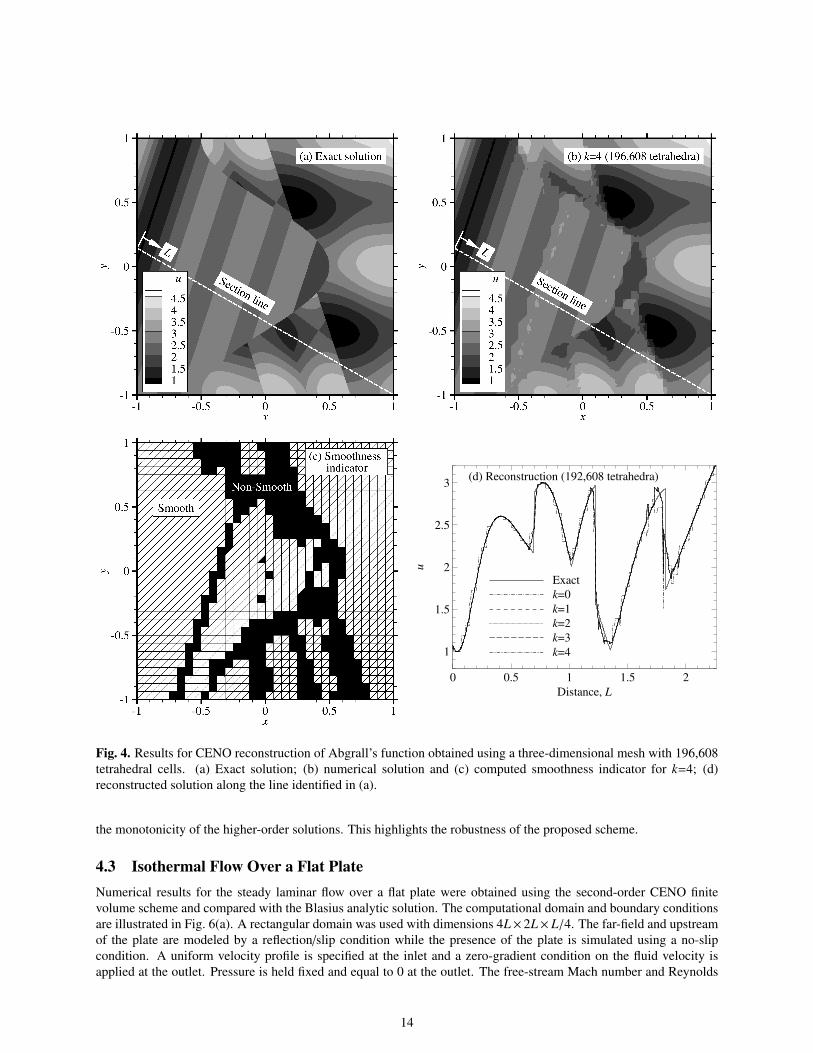
unstructured meshes with k = 4 is compared with the exact solution in Figs. 4(a) and 4(b). The CENO scheme isable to accurately reconstruct the Abgrall function even on a relatively coarse mesh of only 196,608 tetrahedral cellswithout producing spurious oscillations. For this mesh, there is only approximately 58 cells in each direction with anaverage edge length of 0.03. The smoothness indicator, illustrated in Fig. 4(c), correctly identified the discontinuitiesin both f (r) and ∂ f (r)/∂x.
The reconstructed solution obtained with k=0 to k=4 and 196,608 tetrahedral cells along a line is illustrated inFig. 4(d). The proposed CENO scheme is able to ensure oscillation-free solutions despite the large discontinuitiesobserved. The spikes observed in the numerical solution occur when the line intersects the faces between cells at acuteangles.
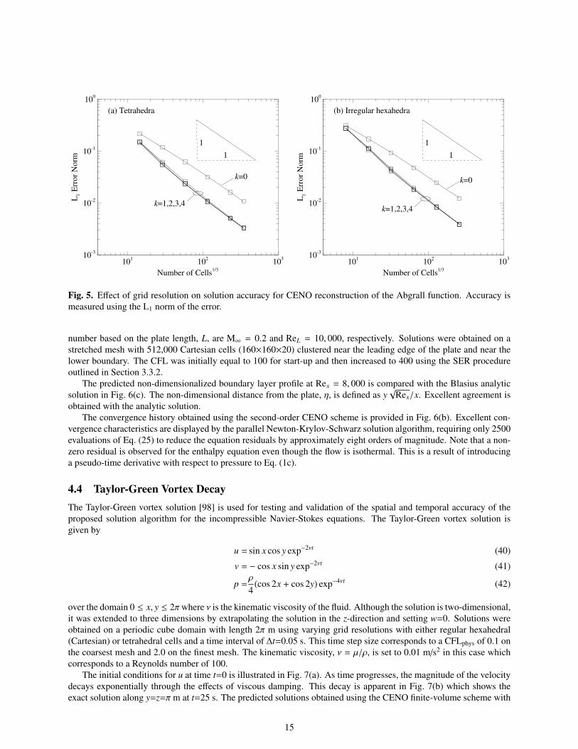
The effect of mesh resolution on the L1 norm of the solution error is shown in Fig. 5 for tetrahedral and irregularhexahedral cells. A large improvement in the error is achieved by increasing k from 0 to 1. This improvementbecomes less pronounced as k is increased further to 4 since a large portion of the domain possesses discontinuousfeatures. An order of accuracy of 1 is expected for all values of k due to discontinuities in the function and the use ofa limited piecewise linear reconstruction in these regions. Nonetheless, the hybrid reconstruction procedure maintains
13
Distance, L
u
0 0.5 1 1.5 2
1
1.5
2
2.5
3
Exact
k=0
k=1
k=2
k=3
k=4
(d) Reconstruction (192,608 tetrahedra)
Fig. 4. Results for CENO reconstruction of Abgrall’s function obtained using a three-dimensional mesh with 196,608tetrahedral cells. (a) Exact solution; (b) numerical solution and (c) computed smoothness indicator for k=4; (d)reconstructed solution along the line identified in (a).
the monotonicity of the higher-order solutions. This highlights the robustness of the proposed scheme.
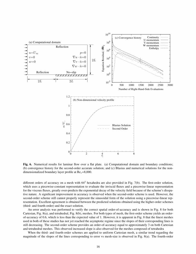
4.3 Isothermal Flow Over a Flat PlateNumerical results for the steady laminar flow over a flat plate were obtained using the second-order CENO finitevolume scheme and compared with the Blasius analytic solution. The computational domain and boundary conditionsare illustrated in Fig. 6(a). A rectangular domain was used with dimensions 4L× 2L× L/4. The far-field and upstreamof the plate are modeled by a reflection/slip condition while the presence of the plate is simulated using a no-slipcondition. A uniform velocity profile is specified at the inlet and a zero-gradient condition on the fluid velocity isapplied at the outlet. Pressure is held fixed and equal to 0 at the outlet. The free-stream Mach number and Reynolds
14
Number of Cells1/3
L1 E
rror
Norm
101
102
103
103
102
101
100
k=0
k=1,2,3,4
(a) Tetrahedra
1
1
Number of Cells1/3
L1 E
rror
Norm
101
102
103
103
102
101
100
k=0
k=1,2,3,4
(b) Irregular hexahedra
1
1
Fig. 5. Effect of grid resolution on solution accuracy for CENO reconstruction of the Abgrall function. Accuracy ismeasured using the L1 norm of the error.
number based on the plate length, L, are M∞ = 0.2 and ReL = 10, 000, respectively. Solutions were obtained on astretched mesh with 512,000 Cartesian cells (160×160×20) clustered near the leading edge of the plate and near thelower boundary. The CFL was initially equal to 100 for start-up and then increased to 400 using the SER procedureoutlined in Section 3.3.2.
The predicted non-dimensionalized boundary layer profile at Rex = 8, 000 is compared with the Blasius analyticsolution in Fig. 6(c). The non-dimensional distance from the plate, η, is defined as y
√Rex/x. Excellent agreement is
obtained with the analytic solution.The convergence history obtained using the second-order CENO scheme is provided in Fig. 6(b). Excellent con-
vergence characteristics are displayed by the parallel Newton-Krylov-Schwarz solution algorithm, requiring only 2500evaluations of Eq. (25) to reduce the equation residuals by approximately eight orders of magnitude. Note that a non-zero residual is observed for the enthalpy equation even though the flow is isothermal. This is a result of introducinga pseudo-time derivative with respect to pressure to Eq. (1c).
4.4 Taylor-Green Vortex DecayThe Taylor-Green vortex solution [98] is used for testing and validation of the spatial and temporal accuracy of theproposed solution algorithm for the incompressible Navier-Stokes equations. The Taylor-Green vortex solution isgiven by
u = sin x cos y exp−2νt (40)
v = − cos x sin y exp−2νt (41)
p =ρ
4(cos 2x + cos 2y) exp−4νt (42)
over the domain 0 ≤ x, y ≤ 2πwhere ν is the kinematic viscosity of the fluid. Although the solution is two-dimensional,it was extended to three dimensions by extrapolating the solution in the z-direction and setting w=0. Solutions wereobtained on a periodic cube domain with length 2π m using varying grid resolutions with either regular hexahedral(Cartesian) or tetrahedral cells and a time interval of ∆t=0.05 s. This time step size corresponds to a CFLphys of 0.1 onthe coarsest mesh and 2.0 on the finest mesh. The kinematic viscosity, ν = µ/ρ, is set to 0.01 m/s2 in this case whichcorresponds to a Reynolds number of 100.
The initial conditions for u at time t=0 is illustrated in Fig. 7(a). As time progresses, the magnitude of the velocitydecays exponentially through the effects of viscous damping. This decay is apparent in Fig. 7(b) which shows theexact solution along y=z=π m at t=25 s. The predicted solutions obtained using the CENO finite-volume scheme with
15
Reflection No−slip
Reflection
(a) Computational domain
u=U∞
w=0
v=0
2L 2L
2L
p=0
∇u · n=0
∇v · n=0
∇w · n=0
10-2
100
102
104
106
108
1010
0 500 1000 1500 2000 2500 3000
Equat
ion R
esid
ual
, ||R
|| 2
Number of Right-Hand-Side Evaluations
(c) Convergence history ContinuityU-momentumV-momentumW-momentum
Enthalpy
u /
U
0 2 4 6 80
0.2
0.4
0.6
0.8
1
1.2
Blasius Solution
Second Order
(b) Nondimensional velocity profile
Fig. 6. Numerical results for laminar flow over a flat plate. (a) Computational domain and boundary conditions;(b) convergence history for the second-order accurate solution; and (c) Blasius and numerical solutions for the non-dimensionalized boundary layer profile at Rex=8,000.
different orders of accuracy on a mesh with 643 hexahedra are also provided in Fig. 7(b). The first-order solution,which uses a piecewise-constant representation to evaluate the inviscid fluxes and a piecewise-linear representationfor the viscous fluxes, greatly over-predicts the exponential decay of the velocity field because of the scheme’s disspa-tive nature. A significant improvement in accuracy is observed when the second-order scheme is used. However, thesecond-order scheme still cannot properly represent the sinusoidal form of the solution using a piecewise-linear rep-resentation. Excellent agreement is obtained between the predicted solutions obtained using the higher-order schemes(third- and fourth-order) and the exact solution.
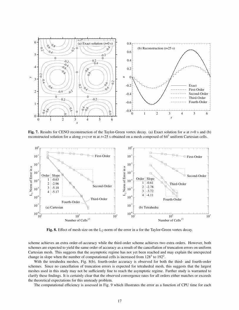
An error analysis was performed to verify the correct spatial order-of-accuracy and is shown in Fig. 8 for bothCartesian, Fig. 8(a), and tetrahedral, Fig. 8(b), meshes. For both types of mesh, the first-order scheme yields an order-of-accuracy of 0.6, which is less than the expected value of 1. However, it is apparent in Fig. 8 that the finest meshesused in both of these studies has not yet reached the asymptotic regime since the slopes of their corresponding lines isstill decreasing. The second-order scheme provides an order-of-accuracy equal to approximately 3 on both Cartesianand tetrahedral meshes. This observed increased slope is also observed for the meshes composed of tetrahedra
When the third- and fourth-order schemes are applied to uniform Cartesian mesh, a similar trend regarding themagnitude of the slopes of the lines corresponding to error vs mesh-size is observed in Fig. 8(a). The fourth-order
16
0.8
0.6
0.6
0.6
0.6
0.4 0
.4
0.4
0.4
0.4
0.4
0.4
0.2
0.2
0.2
0.2
0.2
0.2
0
0
0
0
0
0
0
0
0
0.2
0.2
0.2
0.2
0.2
0.2
0.4
0.4
0.4
0.4
0.4
0.4
0.6
0.6
0.6
0.6
0.8
0.8
0.8
x
y
0 1 2 3 4 5 60
1
2
3
4
5
6 (a) Exact solution (t=0 s)
x
u
0 1 2 3 4 5 60.8
0.6
0.4
0.2
0
0.2
0.4
0.6
0.8
Exact
FirstOrder
SecondOrder
ThirdOrder
FourthOrder
(b) Reconstruction (t=25 s)
Fig. 7. Results for CENO reconstruction of the Taylor-Green vortex decay. (a) Exact solution for u at t=0 s and (b)reconstructed solution for u along y=z=π m at t=25 s obtained on a mesh composed of 643 uniform Cartesian cells.
Number of Cells1/3
L2 N
orm
of
Err
or
in u
101
102
10310
8
107
106
105
104
103
102
101
100
Order Slope
1 0.63
2 2.96
3 5.18
4 5.17
FirstOrder
SecondOrder
ThirdOrderFourthOrder
(a) Cartesian
Number of Cells1/3
L2 N
orm
of
Err
or
in u
101
102
10310
8
107
106
105
104
103
102
101
100
Order Slope
1 0.61
2 2.78
3 3.72
4 4.11
FirstOrder
SecondOrder
ThirdOrder
FourthOrder
(b) Tetrahedra
Fig. 8. Effect of mesh size on the L2-norm of the error in u for the Taylor-Green vortex decay.
scheme achieves an extra order-of-accuracy while the third-order scheme achieves two extra orders. However, bothschemes are expected to yield the same order of accuracy as a result of the cancellation of truncation errors on uniformCartesian mesh. This suggests that the asymptotic regime has not yet been reached and may explain the unexpectedchange in slope when the number of computational cells is increased from 1283 to 1922.
With the tetrahedra meshes, Fig. 8(b), fourth-order accuracy is observed for both the third- and fourth-orderschemes. Since no cancellation of truncation errors is expected for tetrahedral mesh, this suggests that the largestmeshes used in this study may not be sufficiently fine to reach the asymptotic regime. Further study is warranted toclarify these findings. It is certainly clear that the observed convergence rates for all orders either matches or exceedsthe theoretical expectations for this unsteady problem.
The computational efficiency is assessed in Fig. 9 which illustrates the error as a function of CPU time for each
17
CPU Time (s)
L2 N
orm
of
Err
or
in u
102
103
104
105
106
107
108
10910
8
107
106
105
104
103
102
101
100
FirstOrder
SecondOrder
ThirdOrder
FourthOrder
(a) Cartesian
CPU Time (s)
L2 N
orm
of
Err
or
in u
102
103
104
105
106
107
108
10910
8
107
106
105
104
103
102
101
100
FirstOrder
SecondOrder
ThirdOrderFourthOrder
(b) Tetrahedra
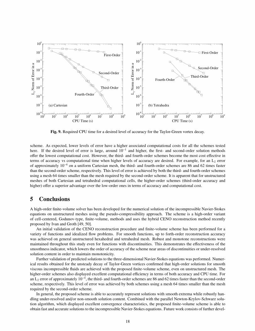
Fig. 9. Required CPU time for a desired level of accuracy for the Taylor-Green vortex decay.
scheme. As expected, lower levels of error have a higher associated computational costs for all the schemes testedhere. If the desired level of error is large, around 10−1 and higher, the first- and second-order solution methodsoffer the lowest computational cost. However, the third- and fourth-order schemes become the most cost effective interms of accuracy vs computational time when higher levels of accuracy are desired. For example, for an L2 errorof approximately 10−4 on a uniform Cartesian mesh, the third- and fourth-order schemes are 86 and 62 times fasterthan the second-order scheme, respectively. This level of error is achieved by both the third- and fourth-order schemesusing a mesh 64 times smaller than the mesh required by the second-order scheme. It is apparent that for unstructuredmeshes of both Cartesian and tetrahedral computational cells, the higher-order schemes (third-order accuracy andhigher) offer a superior advantage over the low-order ones in terms of accuracy and computational cost.
5 ConclusionsA high-order finite-volume solver has been developed for the numerical solution of the incompressible Navier-Stokesequations on unstructured meshes using the pseudo-compressibility approach. The scheme is a high-order variantof cell-centered, Godunov-type, finite-volume, methods and uses the hybrid CENO reconstruction method recentlyproposed by Ivan and Groth [49, 50].
An initial validation of the CENO reconstruction procedure and finite-volume scheme has been performed for avariety of functions and idealized flow problems. For smooth functions, up to forth-order reconstruction accuracywas achieved on general unstructured hexahedral and tetrahedral mesh. Robust and monotone reconstructions weremaintained throughout this study even for functions with discontinuities. This demonstrates the effectiveness of thesmoothness indicator, which lowers the order of accuracy of the scheme near areas of discontinuities or under-resolvedsolution content in order to maintain monotonicity.
Further validation of predicted solutions to the three-dimensional Navier-Stokes equations was performed. Numer-ical results obtained for the unsteady decay of Taylor-Green vortices confirmed that high-order solutions for smoothviscous incompressible fluids are achieved with the proposed finite-volume scheme, even on unstructured mesh. Thehigher-order schemes also displayed excellent computational efficiency in terms of both accuracy and CPU time. Foran L2 error of approximately 10−4, the third- and fourth-order schemes are 86 and 62 times faster than the second-orderscheme, respectively. This level of error was achieved by both schemes using a mesh 64 times smaller than the meshrequired by the second-order scheme.
In general, the proposed scheme is able to accurately represent solutions with smooth extrema while robustly han-dling under-resolved and/or non-smooth solution content. Combined with the parallel Newton-Krylov-Schwarz solu-tion algorithm, which displayed excellent convergence characteristics, the proposed finite-volume scheme is able toobtain fast and accurate solutions to the incompressible Navier-Stokes equations. Future work consists of further devel-
18
opment and validation of the proposed Newton-Krylov-Schwarz CENO algorithm for three-dimensional unstructuredmeshes. This includes applying the pseudo-compressibility approach to more complex flows, such as the large-eddysimulation of turbulent flames, and incorporating a multi-block adaptive mesh refinement (AMR) algorithm [99–102].The applicability of CENO to AMR and the substantial benefits in terms of accuracy and computational savings havealready been demonstrated for body-fitted multi-block meshes [49, 50].
AcknowledgmentsFinancial support for the research described herein was provided by MITACS (Mathematics of Information Technol-ogy and Complex Systems) Network, part of the Networks of Centres of Excellence (NCE) program funded by theCanadian government, as well as by Rolls-Royce Canada Inc. This funding is gratefully acknowledged with manythanks. Computational resources for performing all of the calculations reported herein were provided by the SciNetHigh Performance Computing Consortium at the University of Toronto and Compute/Calcul Canada through fundingfrom the Canada Foundation for Innovation (CFI) and the Province of Ontario, Canada.
References[1] D. Drikakis and W. Rider. High-resolution methods for incompressible and low-speed flows. Springer-Verlag,
Berlin, Heidelberg, 2005.
[2] D. Kwak, C. Kiris, and J. Housman. Comput. Fluids, 41(1):51–64, 2011.
[3] S.V. Patankar and D.B. Spalding. Int. J. Heat Mass Transfer, 15(10):1787–1806, 1972.
[4] C.M. Rhie and W.L. Chow. AIAA J., 21(11):1525–1532, 1983.
[5] N.N. Yanenko. The Method of Fractional Steps. Springer-Verlag, Berlin, 1971.
[6] J. Kim and P. Moin. J. Comput. Phys., 59(2):308–323, 1985.
[7] H. Fasel. J. Fluid Mech., 78(2):355–383, 1976.
[8] S.C.R. Dennis, D.B. Ingham, and R.N. Cook. J. Comput. Phys., 33(3):325–339, 1979.
[9] A.J. Chorin. J. Comput. Phys., 2(1):12–26, 1967.
[10] B. Van Leer, W.T. Lee, and P.L. Roe. AIAA Paper 91-1552, 1991.
[11] Y.H. Choi and C.L. Merkle. J. Comput. Phys., 105(2):207–223, 1993.
[12] E. Turkel. Appl. Numer. Math., 12(1-3):257–284, 1993.
[13] J.M. Weiss and W.A. Smith. AIAA J., 33(11):2050–2057, 1995.
[14] E. Turkel, R. Radespiel, and N. Kroll. Comput. Fluids, 26(6):613–634, 1997.
[15] S. Venkateswaran, M. Deshpande, and C.L. Merkle. The application of preconditioning to reacting flow com-putations. In 12th AIAA Computational Fluid Dynamics Conference, San Diego, CA, Jun. 19-22 1995. AIAApaper 1995-1673.
[16] J.L. Steger and P. Kutler. AIAA J., 15(4):581–590, 1977.
[17] D. Kwak, J.L.C. Chang, S.P. Shanks, and S.R. Chakravarthy. AIAA J., 24(3):390–396, 1986.
[18] E. Turkel. J. Comput. Phys., 72(2):277–298, 1987.
[19] S.E. Rogers, D. Kwak, and U. Kaul. Appl. Math. Model., 11(1):35–44, 1987.
[20] C. Kiris, D. Kwak, S. Rogers, and I.D. Chang. J. Biomed. Eng., 119(4):452–460, 1997.
19
[21] S.E. Rogers and D. Kwak. AIAA J., 28(2):253–262, 1990.
[22] S.E. Rogers, D. Kwak, and C. Kiris. AIAA J., 29(4):603–610, 1991.
[23] Z. Qian and J. Zhang. Int. J. Numer. Meth. Fluids, 69(7):1165–1185, 2012.
[24] J.L.C. Chang and D. Kwak. AIAA Paper 84-0252, 1984.
[25] S. Pirozzoli. J. Comput. Phys., 219(2):489–497, 2006.
[26] A. Harten, B. Engquist, S. Osher, and S.R. Chakravarthy. J. Comput. Phys., 71(2):231–303, 1987.
[27] W.J. Coirier and K.G. Powell. AIAA J., 34(5):938–945, May 1996.
[28] T.J. Barth. AIAA Paper 93-0668, 1993.
[29] R. Abgrall. J. Comput. Phys., 114:45–58, 1994.
[30] T. Sonar. Comp. Meth. Appl. Mech. Eng., pages 140–157, 1997.
[31] C.F. Ollivier-Gooch. J. Comput. Phys., 133:6–17, 1997.
[32] G.S. Jiang and C.W. Shu. J. Comput. Phys., 126(1):202–228, 1996.
[33] D. Stanescu and W. Habashi. AIAA J., 36:1413–1416, 1998.
[34] O. Friedrich. J. Comput. Phys., 144:194–212, 1998.
[35] C. Hu and C.W. Shu. J. Comput. Phys., 150:97–127, 1999.
[36] C.F. Ollivier-Gooch and M. Van Altena. J. Comput. Phys., 181(2):729–752, 2002.
[37] A. Nejat and C. Ollivier-Gooch. J. Comput. Phys., 227(4):2582–2609, 2008.
[38] B. Cockburn and C.W. Shu. Math. Comp., 52:411, 1989.
[39] B. Cockburn, S. Hou, and C.W. Shu. J. Comput. Phys., 54:545, 1990.
[40] R. Hartmann and P. Houston. J. Comput. Phys., 183:508–532, 2002.
[41] H. Luo, J.D. Baum, and R. Löhner. J. Comput. Phys., 225:686–713, 2007.
[42] G. Gassner, F. Lörcher, and C.D. Munz. J. Comput. Phys., 224(2):1049–1063, 2007.
[43] Z.J. Wang. J. Comput. Phys., 178:210–251, 2002.
[44] Z.J. Wang and Y. Liu. J. Comput. Phys., 179:665–697, 2002.
[45] Z.J. Wang, L. Zhang, and Y. Liu. High-order spectral volume method for 2d euler equations. Paper 2003–3534,AIAA, June 2003.
[46] Z.J. Wang and Y. Liu. Journal of Scientific Computing, 20(1):137–157, 2004.
[47] Y. Sun, Z.J. Wang, and Y. Liu. J. Comput. Phys., 215(1):41–58, 2006.
[48] A. Haselbacher. AIAA paper 2005-0879, 2005.
[49] L. Ivan and C.P.T. Groth. AIAA paper 2007-4323, 2007.
[50] L. Ivan and C.P.T. Groth. AIAA paper 2011-0367, 2011.
[51] S.D. McDonald, M.R.J. Charest, and C.P.T. Groth. High-order CENO finite-volume schemes for multi-blockunstructured mesh. In 20th AIAA Computational Fluid Dynamics Conference, Honolulu, Hawaii, June 27–302011. AIAA-2011-3854.
20
[52] S.E. Rogers and D. Kwak. Appl. Numer. Math., 8(1):43–64, 1991.
[53] Y.N. Chen, S.C. Yang, and J.Y. Yang. Int. J. Numer. Meth. Fluids, 31(4):747–765, 1999.
[54] S.E. Rogers, J.L.C. Chang, and D. Kwak. J. Comput. Phys., 73(2):364–379, 1987.
[55] S. Yoon and D. Kwak. AIAA Paper 89-1964, 1989.
[56] R.S. Dembo, S.C. Eisenstat, and T. Steihaug. SIAM J. Numer. Anal., 19(2):400–408, 1982.
[57] T.F. Chan and K.R. Jackson. SIAM J. Sci. Stat. Comput., 5(3):533–542, 1984.
[58] P.N. Brown and Y. Saad. SIAM J. Sci. Stat. Comput., 11(3):450–481, 1990.
[59] D.A. Knoll and D.E. Keyes. J. Comput. Phys., 193(2):357–397, 2004.
[60] D.A. Knoll, V.A. Mousseau, L. ChacÃsn, and J. Reisner. J. Comput. Phys., 25(1):213–230, 2005.
[61] D. Pan and C.. Chang. Int. J. Numer. Meth. Fluids, 33(2):203–222, 2000.
[62] L. Qian, D.M. Causon, D.M. Ingram, and C.G. Mingham. J. Hydraul. Eng., 129(9):688–696, 2003.
[63] U. Riedel. Combust. Sci. Tech., 135(1-6):99–116, 1998.
[64] E. Shapiro and D. Drikakis. J. Comput. Phys., 210(2):584–607, 2005.
[65] M. Azhdarzadeh and S.E. Razavi. J. Appl. Sci., 8(18):3183–3190, 2008.
[66] S.L. Chang and K.T. Rhee. Int. Commun. Heat Mass Transfer, 11(5):451–455, 1984.
[67] A. Jameson. AIAA paper 1991-1596, 1991.
[68] C.L. Merkle and M. Athavale. AIAA paper 87-1137, 1987.
[69] W.Y. Soh and J.W. Goodrich. J. Comput. Phys., 79(1):113–134, 1988.
[70] Z. Qian, J. Zhang, and C. Li. Science China: Physics, Mechanics and Astronomy, 53(11):2090–2102, 2010.
[71] H. Lee and S. Lee. Int. J. Aeronaut. Space Sci., 12(4):318–330, 2011.
[72] A.G. Malan, R.W. Lewis, and P. Nithiarasu. Int. J. Numer. Meth. Engin., 54(5):695–714, 2002.
[73] A.G. Malan, R.W. Lewis, and P. Nithiarasu. Int. J. Numer. Meth. Engin., 54(5):715–729, 2002.
[74] R.L. Naff, T.F. Russell, and J.D. Wilson. Shape functions for three-dimensional control-volume mixed finite-element methods on irregular grids, volume 47 of Developments in Water Science, pages 359–366. Elsevier,2002.
[75] R. Naff, T. Russell, and J. Wilson. Computat. Geosci., 6:285–314, 2002.
[76] C.A. Felippa. Eng. Computation., 21(8):867–890, 2004.
[77] L. Ivan. Development of high-order CENO finite-volume schemes with block-based adaptive mesh refinement.PhD thesis, University of Toronto, 2011.
[78] C.L. Lawson and R.J. Hanson. Solving least squares problems. Prentice-Hall, 1974.
[79] D.J. Mavriplis. AIAA paper 2003-3986, 2003.
[80] J.S. Park, S.H. Yoon, and C. Kim. J. Comput. Phys., 229(3):788–812, 2010.
[81] V. Venkatakrishnan. AIAA Paper 93-0880, 1993.
[82] P.L. Roe. J. Comput. Phys., 43:357–372, 1981.
21
[83] P.L. Roe and J. Pike. Efficient construction and utilisation of approximate Riemann solutions. In R. Glowinskiand J.L. Lions, editors, Computing Methods in Applied Science and Engineering, volume VI, pages 499–518,Amsterdam, 1984. North-Holland.
[84] S.R. Mathur and J.Y. Murthy. Numer. Heat Transfer, Part B, 31(2):195–215, 1997.
[85] G. Karypis and K. Schloegel. http://www.cs.umn.edu/~metis, 2011.
[86] W. Gropp, E. Lusk, and A. Skjellum. Using MPI. MIT Press, Cambridge, Massachussets, 1999.
[87] C.P.T. Groth and S.A. Northrup. Parallel implicit adaptive mesh refinement scheme for body-fitted multi-blockmesh. In 17th AIAA Computational Fluid Dynamics Conference, Toronto, Ontario, Canada, 6-9 June 2005.AIAA paper 2005-5333.
[88] M.R.J. Charest, C.P.T. Groth, and Ö.L. Gülder. Combust. Theor. Modelling, 14(6):793–825, 2010.
[89] M.R.J. Charest, C.P.T. Groth, and Ö.L. Gülder. J. Comput. Phys., 231(8):3023–3040, 2012.
[90] Y. Saad and M.H. Schultz. SIAM J. Sci. Stat. Comput., 7(3):856–869, 1986.
[91] Y. Saad. SIAM J. Sci. Stat. Comput., 10(6):1200–1232, 1989.
[92] Y. Saad. Iterative Methods for Sparse Linear Systems. PWS Publishing Company, Boston, 1996.
[93] E. Cuthill and J. McKee. Reducing the bandwidth of sparse symmetric matrices. In Proceedings of the 196924th National Conference, ACM ’69, pages 157–172, New York, NY, USA, 1969. ACM.
[94] W.A. Mulder and B. Van Leer. J. Comput. Phys., 59:232–246, 1985.
[95] M. Tabesh and D.W. Zingg. Efficient implicit time-marching methods using a Newton-Krylov algorithm. In47th AIAA Aerospace Sciences Meeting and Exhibit, Orlando, Florida, 5-8 January 2009. AIAA paper 2009-0164.
[96] A. Genz and R. Cools. ACM Trans. Math. Softw., 29(3):297–308, 2003.
[97] R. Cools and A. Haegemans. ACM Trans. Math. Softw., 29(3):287–296, 2003.
[98] G.I. Taylor and A.E. Green. Proc. Royal Soc. London A, 158(895):499–521, 1937.
[99] J.S. Sachdev, C.P.T. Groth, and J.J. Gottlieb. Int. J. Comput. Fluid Dyn., 19(2):159–177, 2005.
[100] X. Gao and C.P.T. Groth. Int. J. Comput. Fluid Dyn., 20(5):349–357, 2006.
[101] X. Gao and C.P.T. Groth. J. Comput. Phys., 229(9):3250–3275, 2010.
[102] X. Gao, S. Northrup, and C.P.T. Groth. Prog. Comput. Fluid. Dy., 11(2):76–95, 2011.
22