High-PerformanceAsynchronous Pipelines:An OverviewSteven M. NowickColumbia University

Montek SinghUniversity of North Carolina at Chapel Hill

!ONE OF THE FOUNDATIONS of high-performance

digital system design is the use of pipelining. In syn-

chronous systems, for several decades, pipelining

has been the fundamental technique used to increase

parallelism and hence boost system throughput!!whether for high-performance processors, multime-

dia and graphics units, or signal processors.

This article provides an overview of pipelining in

asynchronous, or clockless, digital systems. We do

not attempt an exhaustive coverage, but rather intro-

duce the basics of several leading representative

styles. These pipelines naturally fall into two classes:

those that use static logic versus those that use

dynamic logic for the data path. Each class tends to

use a distinct approach for its control and data

storage. For static logic, we introduce the classic

micropipeline of Sutherland,1 along with two high-

performance variants: Mousetrap2 (which uses a stan-

dard cell design) and GasP3 (which uses a custom de-

sign). For dynamic logic, we present the classic PS0

pipeline of Williams and Horowitz,4,5 along with two

high-performance variants: the precharge half-buffer

(PCHB) pipeline6 (which provides greater timing

robustness) and the high-capacity (HC) pipeline7

(which provides double the storage capacity).

We also briefly discuss design trade-

offs, performance evaluation, system-

level analysis and optimization tech-

niques, CAD tool support, testing,

and recent industrial and academic

applications.

Applications of pipeliningin asynchronous systems

For synchronous systems, pipelining

is a straightforward technique: complex

function blocks are subdivided into smaller blocks,

registers are inserted to separate them, and the global

clock is applied to all registers. In contrast, for asyn-

chronous systems, there is no global clock. Therefore,

a protocol for the interaction of neighboring stages

must be defined, as well as choices of data encoding

and storage elements. In addition, an explicit distrib-

uted control structure must be designed. Together,

this ensemble constitutes a template or skeleton for

coordinating the blocks of a pipelined asynchronous

system.

Several leading processors from the 1950s and

1960s used asynchronous circuits extensively, includ-

ing the Illiac and Illiac II (University of Illinois), the

Atlas and MU-5 (University of Manchester), and

designs from the Macromodules project (Washington

University, St. Louis).

The basic concept and design of an asynchronous

pipeline were presented by David Muller in his semi-

nal paper from 1963.8 Since then, asynchronous pipe-

lines have had broad application, from the early

commercial graphics and flight simulation systems

of Evans & Sutherland, whose LDS-1 (Line Drawing

System-1) was first shipped to Bolt, Beranek and

Newman (BBN) in 1969, to the foundational

Asynchronous Design

Editor’s note:

Pipelining is a key element of high-performance design. Distributed synchroni-

zation is at the same time one of the key strengths and one of the major difficul-

ties of asynchronous pipelining. It automatically provides elasticity and

on-demand power consumption. This tutorial provides an overview of the

best-in-class asynchronous pipelining methods that can be used to fully exploit

the advantages of this design style, covering both static and dynamic logic

implementations.

!!Luciano Lavagno, Politecnico di Torino

0740-7475/11/$26.00 "c 2011 IEEE Copublished by the IEEE CS and the IEEE CASS IEEE Design & Test of Computers8

[3B2-9] mdt2011050008.3d 5/9/011 11:54 Page 8

approaches of Chuck Seitz.9 More recently, high-

performance asynchronous pipelines have been

used commercially in

! Sun’s UltraSparc IIIi computers for fast memory

access;

! the Speedster FPGAs of Achronix Semiconductor

(http://www.achronix.com), which, at a peak

performance of 1.5 GHz, are currently claimed

as the world’s fastest;10 and

! the Nexus Ethernet switch chips of Fulcrum

Microsystems, an asynchronous start-up com-

pany recently acquired by Intel11 (http://www.

fulcrummicro.com).

Asynchronous pipelines have also been used ex-

perimentally at IBM Research for a low-latency finite-

impulse response (FIR) filter chip.12

Asynchronous vs. synchronouspipelines

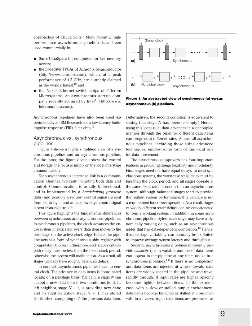
Figure 1 shows a highly simplified view of a syn-

chronous pipeline and an asynchronous pipeline.

For the latter, the figure doesn’t show the control

and storage; the focus is simply on the local interstage

communication.

Each asynchronous interstage link is a communi-

cation channel, typically including both data and

control. Communication is usually bidirectional,

and is implemented by a handshaking protocol:

data (and possibly a request control signal) is sent

from left to right, and an acknowledge control signal

is sent from right to left.

This figure highlights the fundamental differences

between synchronous and asynchronous pipelines.

In synchronous pipelines, the clock advances the en-

tire system in lock step: every data item moves to the

next stage on the active clock edge. Hence, the pipe-

line acts as a form of synchronous shift register with

computationblocks. Furthermore, each stage’s critical-

path delay must be less than the fixed clock period,

otherwise the system will malfunction. As a result, all

stages typically have roughly balanced delays.

In contrast, asynchronous pipelines have no cen-

tral clock. The advance of data items is coordinated

locally, on a per-stage basis. Typically, a stage N can

accept a new data item if two conditions hold: its

left neighbor, stage N ! 1, is providing new data;

and its right neighbor, stage N # 1, has stored

(or finished computing on) the previous data item.

(Alternatively, the second condition is equivalent to

stating that stage N has become empty.) Hence,

using this local rule, data advances in a decoupled

manner through the pipeline: different data items

can progress at different rates. Almost all asynchro-

nous pipelines, including those using advanced

techniques, employ some form of this local rule

for data movement.

The asynchronous approach has four important

features in providing design flexibility and modularity.

First, stages need not have equal delays. In most syn-

chronous systems, the worst-case stage delay must be

less than the clock period, and all stages operate at

the same fixed rate. In contrast, in an asynchronous

system, although balanced stages tend to provide

the highest system performance, this balance is not

a requirement for correct operation. As a result, stages

of widely different static delays can be concatenated

to form a working system. In addition, in some asyn-

chronous pipeline styles, each stage may have a dy-

namically varying delay, such as an asynchronous

adder that has data-dependent completion.13 Hence,

this per-stage variability can naturally be exploited

to improve average system latency and throughput.

Second, asynchronous pipelines inherently pro-

vide elasticity (i.e., a variable number of data items

can appear in the pipeline at any time, unlike in a

synchronous pipeline).1,8 If there is no congestion

and data items are injected at wide intervals, data

items are widely spaced in the pipeline and travel

rapidly through. If input rates are higher, spacing

becomes tighter between items. In the extreme

case, with a slow or stalled output environment,

data items become bunched or stalled at close inter-

vals. In all cases, input data items are processed as

(a)

(b)

Global clock

Synchronous

No global clock Asynchronous

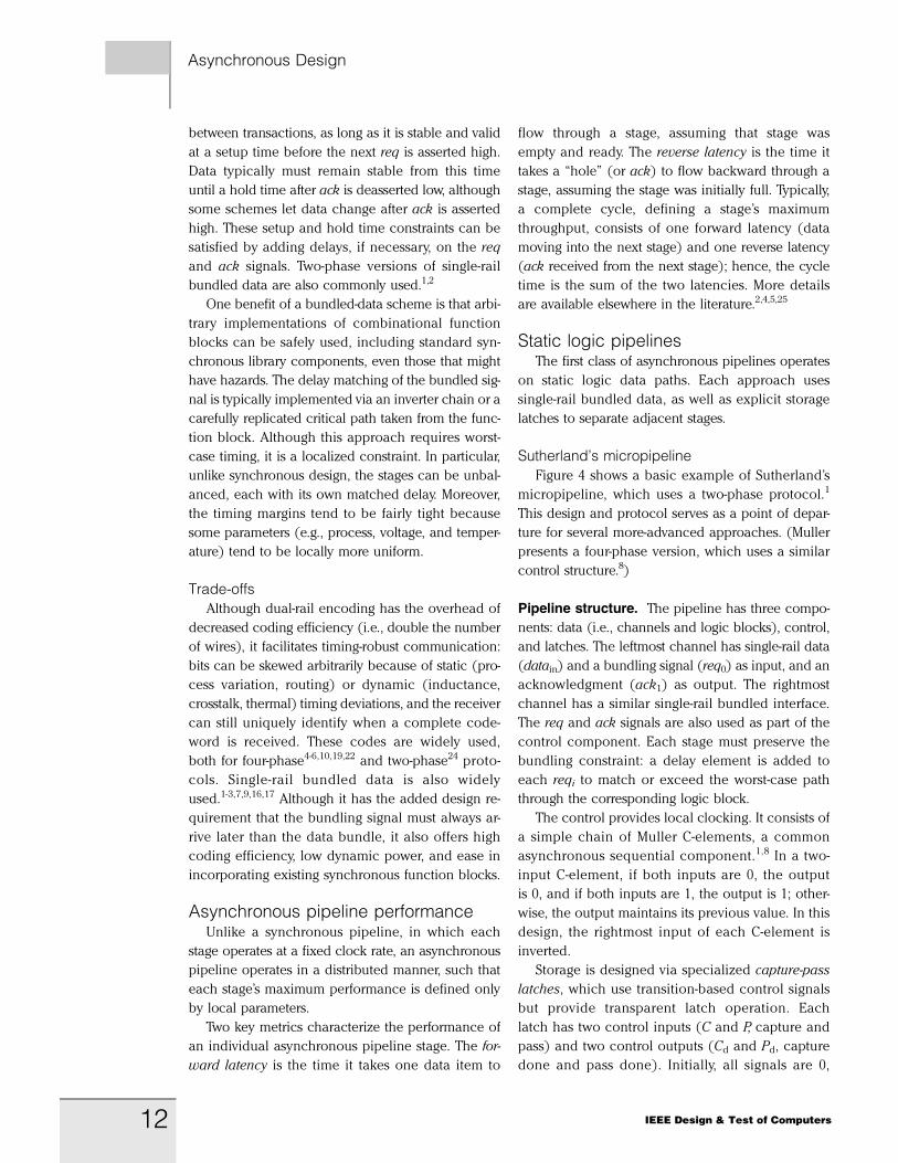
Figure 1. An abstracted view of synchronous (a) versus

asynchronous (b) pipelines.

9September/October 2011

[3B2-9] mdt2011050008.3d 5/9/011 11:54 Page 9

they arrive, even with an unknown or irregular arrival

rate; there is no wait for a clock edge. Hence, the

intertoken spacing and the throughput rate are deter-

mined dynamically.

Third, asynchronous pipelines automatically pro-

vide flow control. A handshaking protocol inher-

ently offers underflow and overflow protection,

even in variable-speed environments. In contrast,

synchronous pipelines by default include no flow

control. Synchronous flow control is typically sup-

ported using explicit credit-based techniques

involving extra registers14 or complex decoupled

latch control.15 A stall signal, used for back pres-

sure, must also be synchronized to the clock at

every stage.

Finally, asynchronous pipelines consume dy-

namic power only on demand. That is, switching

activity occurs only when data items are being pro-

cessed; otherwise, stages and their control are qui-

escent. Effectively, this approach achieves the

benefit of automatic clock gating, but without

extra instrumentation, at arbitrary levels of granular-

ity in the design, including under rapidly changing

traffic patterns. Furthermore, asynchronous pipe-

lines inherently obviate the need for global clock

distribution.

Linear and nonlinear pipeline structuresThe focus of this article is on linear pipelines, in

which each stage has a single input channel and a

single output channel. However, to construct com-

plex digital systems with varied topologies, various

other pipeline components are needed, such as par-

allel forks and joins, conditional splits and merges,

arbitration, and loop control structures. These com-

ponents typically involve small extensions to the lin-

ear stages, and their designs are covered extensively

in the literature.2,3,6-8,16,17

Benefits of asynchronous pipelinesThe preceding four features make asynchronous

pipelines highly attractive as a medium for assem-

bling scalable complex systems. An important goal

is to design a pipeline with a throughput compara-

ble to a high-performance synchronous pipeline,

but with lower end-to-end latency, dynamic power

that naturally adapts to the actual traffic, and the

flexibility to handle variable input and output

rates and variable-delay stages. As a result, an

asynchronous pipeline can be reused, without

modification, when interfacing to a large variety of

input and output environments. It can also grace-

fully support dynamic voltage and frequency scal-

ing (DVFS) at its interfaces.

In addition, if mixed-timing interfaces18 or stop-

pable clocks9 are used, asynchronous pipelines

can connect arbitrary, unrelated synchronous

clock domains. Hence, these pipelines can serve

as the foundation for designing globally asynchro-

nous, locally synchronous (GALS) systems. A GALS

approach has been used for several recent pipe-

lined networks on chips (NoCs).11,16,19 Several pipe-

lined asynchronous NoCs have been shown to

provide significantly lower dynamic power and sys-

tem latency than comparable single-clock16 and

multiclock20 NoCs.

Finally, there is increasing interest in using asyn-

chronous pipelines as the organizing structure for

emerging technologies, such as quantum-dot cellular

automata (QCA)21 and carbon nanotubes (CNTs),

whose timing irregularities make fixed-rate clock dis-

tribution extremely difficult.

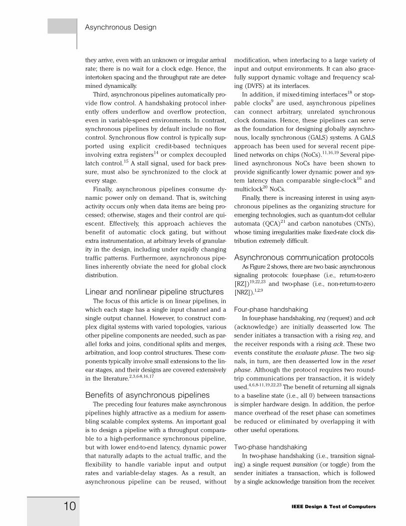
Asynchronous communication protocolsAs Figure 2 shows, there are two basic asynchronous

signaling protocols: four-phase (i.e., return-to-zero

[RZ])19,22,23 and two-phase (i.e., non-return-to-zero

[NRZ]).1,2,9

Four-phase handshakingIn four-phase handshaking, req (request) and ack

(acknowledge) are initially deasserted low. The

sender initiates a transaction with a rising req, and

the receiver responds with a rising ack. These two

events constitute the evaluate phase. The two sig-

nals, in turn, are then deasserted low in the reset

phase. Although the protocol requires two round-

trip communications per transaction, it is widely

used.4,6,8-11,19,22,23 The benefit of returning all signals

to a baseline state (i.e., all 0) between transactions

is simpler hardware design. In addition, the perfor-

mance overhead of the reset phase can sometimes

be reduced or eliminated by overlapping it with

other useful operations.

Two-phase handshakingIn two-phase handshaking (i.e., transition signal-

ing) a single request transition (or toggle) from the

sender initiates a transaction, which is followed

by a single acknowledge transition from the receiver.

Asynchronous Design

10 IEEE Design & Test of Computers

[3B2-9] mdt2011050008.3d 5/9/011 11:54 Page 10

The protocol requires only one

round-trip communication per

transaction. Although hardware

in some cases is more complex,

the throughput and power ben-

efits of a single round-trip com-

munication per transaction

are significant, especially for

long-distance communication.

This approach is also widely

used.1,2,9,12,16

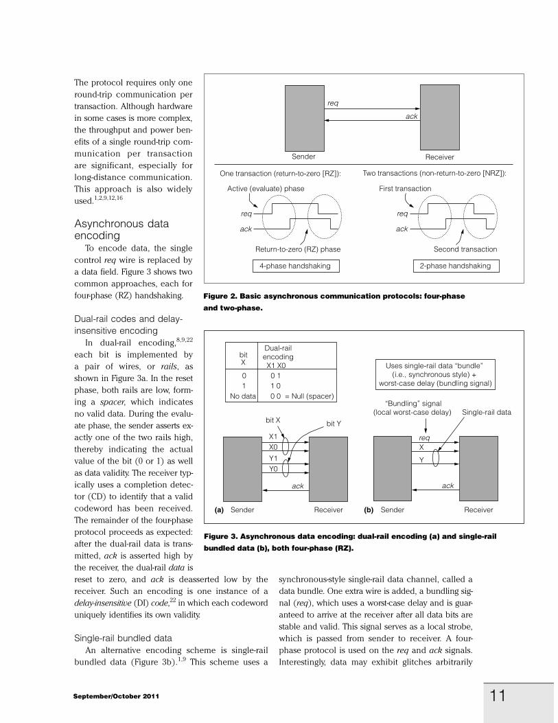
Asynchronous dataencoding

To encode data, the single

control req wire is replaced by

a data field. Figure 3 shows two

common approaches, each for

four-phase (RZ) handshaking.

Dual-rail codes and delay-insensitive encoding

In dual-rail encoding,8,9,22

each bit is implemented by

a pair of wires, or rails, as

shown in Figure 3a. In the reset

phase, both rails are low, form-

ing a spacer, which indicates

no valid data. During the evalu-

ate phase, the sender asserts ex-

actly one of the two rails high,

thereby indicating the actual

value of the bit (0 or 1) as well

as data validity. The receiver typ-

ically uses a completion detec-

tor (CD) to identify that a valid

codeword has been received.

The remainder of the four-phase

protocol proceeds as expected:

after the dual-rail data is trans-

mitted, ack is asserted high by

the receiver, the dual-rail data is

reset to zero, and ack is deasserted low by the

receiver. Such an encoding is one instance of a

delay-insensitive (DI) code,22 in which each codeword

uniquely identifies its own validity.

Single-rail bundled data

An alternative encoding scheme is single-rail

bundled data (Figure 3b).1,9 This scheme uses a

synchronous-style single-rail data channel, called a

data bundle. One extra wire is added, a bundling sig-

nal (req), which uses a worst-case delay and is guar-

anteed to arrive at the receiver after all data bits are

stable and valid. This signal serves as a local strobe,

which is passed from sender to receiver. A four-

phase protocol is used on the req and ack signals.

Interestingly, data may exhibit glitches arbitrarily

Sender Receiver

ack

reqX

Y

Uses single-rail data “bundle” (i.e., synchronous style) +

worst-case delay (bundling signal)

“Bundling” signal(local worst-case delay) Single-rail data

Sender(a) (b)Receiver

ack

Y1 Y0

bit Y

X1 X0

bit X

bit X

Dual-railencoding X1 X0

0 0 1 1 1 0

No data 0 0 = Null (spacer)

Figure 3. Asynchronous data encoding: dual-rail encoding (a) and single-rail

bundled data (b), both four-phase (RZ).

Sender Receiver

req

ack

req

ack

Active (evaluate) phase

Return-to-zero (RZ) phase

4-phase handshaking

One transaction (return-to-zero [RZ]):

req

ack

First transaction

Second transaction

2-phase handshaking

Two transactions (non-return-to-zero [NRZ]):

Figure 2. Basic asynchronous communication protocols: four-phase

and two-phase.

11September/October 2011

[3B2-9] mdt2011050008.3d 5/9/011 11:54 Page 11

between transactions, as long as it is stable and valid

at a setup time before the next req is asserted high.

Data typically must remain stable from this time

until a hold time after ack is deasserted low, although

some schemes let data change after ack is asserted

high. These setup and hold time constraints can be

satisfied by adding delays, if necessary, on the req

and ack signals. Two-phase versions of single-rail

bundled data are also commonly used.1,2

One benefit of a bundled-data scheme is that arbi-

trary implementations of combinational function

blocks can be safely used, including standard syn-

chronous library components, even those that might

have hazards. The delay matching of the bundled sig-

nal is typically implemented via an inverter chain or a

carefully replicated critical path taken from the func-

tion block. Although this approach requires worst-

case timing, it is a localized constraint. In particular,

unlike synchronous design, the stages can be unbal-

anced, each with its own matched delay. Moreover,

the timing margins tend to be fairly tight because

some parameters (e.g., process, voltage, and temper-

ature) tend to be locally more uniform.

Trade-offsAlthough dual-rail encoding has the overhead of

decreased coding efficiency (i.e., double the number

of wires), it facilitates timing-robust communication:

bits can be skewed arbitrarily because of static (pro-

cess variation, routing) or dynamic (inductance,

crosstalk, thermal) timing deviations, and the receiver

can still uniquely identify when a complete code-

word is received. These codes are widely used,

both for four-phase4-6,10,19,22 and two-phase24 proto-

cols. Single-rail bundled data is also widely

used.1-3,7,9,16,17 Although it has the added design re-

quirement that the bundling signal must always ar-

rive later than the data bundle, it also offers high

coding efficiency, low dynamic power, and ease in

incorporating existing synchronous function blocks.

Asynchronous pipeline performanceUnlike a synchronous pipeline, in which each

stage operates at a fixed clock rate, an asynchronous

pipeline operates in a distributed manner, such that

each stage’s maximum performance is defined only

by local parameters.

Two key metrics characterize the performance of

an individual asynchronous pipeline stage. The for-

ward latency is the time it takes one data item to

flow through a stage, assuming that stage was

empty and ready. The reverse latency is the time it

takes a ‘‘hole’’ (or ack) to flow backward through a

stage, assuming the stage was initially full. Typically,

a complete cycle, defining a stage’s maximum

throughput, consists of one forward latency (data

moving into the next stage) and one reverse latency

(ack received from the next stage); hence, the cycle

time is the sum of the two latencies. More details

are available elsewhere in the literature.2,4,5,25

Static logic pipelinesThe first class of asynchronous pipelines operates

on static logic data paths. Each approach uses

single-rail bundled data, as well as explicit storage

latches to separate adjacent stages.

Sutherland’s micropipeline

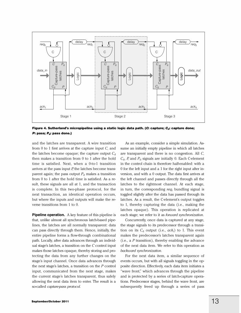
Figure 4 shows a basic example of Sutherland’s

micropipeline, which uses a two-phase protocol.1

This design and protocol serves as a point of depar-

ture for several more-advanced approaches. (Muller

presents a four-phase version, which uses a similar

control structure.8)

Pipeline structure. The pipeline has three compo-

nents: data (i.e., channels and logic blocks), control,

and latches. The leftmost channel has single-rail data

(datain) and a bundling signal (req0) as input, and an

acknowledgment (ack1) as output. The rightmost

channel has a similar single-rail bundled interface.

The req and ack signals are also used as part of the

control component. Each stage must preserve the

bundling constraint: a delay element is added to

each reqi to match or exceed the worst-case path

through the corresponding logic block.

The control provides local clocking. It consists of

a simple chain of Muller C-elements, a common

asynchronous sequential component.1,8 In a two-

input C-element, if both inputs are 0, the output

is 0, and if both inputs are 1, the output is 1; other-

wise, the output maintains its previous value. In this

design, the rightmost input of each C-element is

inverted.

Storage is designed via specialized capture-pass

latches, which use transition-based control signals

but provide transparent latch operation. Each

latch has two control inputs (C and P, capture and

pass) and two control outputs (Cd and Pd, capture

done and pass done). Initially, all signals are 0,

Asynchronous Design

12 IEEE Design & Test of Computers

[3B2-9] mdt2011050008.3d 5/9/011 11:54 Page 12

and the latches are transparent. A wire transition

from 0 to 1 first arrives at the capture input C, and

the latches become opaque; the capture output Cd

then makes a transition from 0 to 1 after the hold

time is satisfied. Next, when a 0-to-1 transition

arrives at the pass input P, the latches become trans-

parent again; the pass output Pd makes a transition

from 0 to 1 after the hold time is satisfied. As a re-

sult, these signals are all at 1, and the transaction

is complete. In this two-phase protocol, for the

next transaction, an identical operation occurs,

but where the inputs and outputs will make the re-

verse transitions from 1 to 0.

Pipeline operation. A key feature of this pipeline is

that, unlike almost all synchronous latch-based pipe-

lines, the latches are all normally transparent: data

can pass directly through them. Hence, initially, the

entire pipeline forms a flow-through combinational

path. Locally, after data advances through an individ-

ual stage’s latches, a transition on the C control input

makes those latches opaque, thereby storing and pro-

tecting the data from any further changes on the

stage’s input channel. Once data advances through

the next stage’s latches, a transition on the P control

input, communicated from the next stage, makes

the current stage’s latches transparent, thus safely

allowing the next data item to enter. The result is a

so-called capture-pass protocol.

As an example, consider a simple simulation. As-

sume an initially empty pipeline in which all latches

are transparent and there is no congestion. All C,

Cd, P, and Pd signals are initially 0. Each C-element

in the control chain is therefore half-enabled: with a

0 for the left input and a 1 for the right input after in-

version, and with a 0 output. The data first arrives at

the left channel and passes directly through all the

latches to the rightmost channel. At each stage,

in turn, the corresponding reqi bundling signal is

toggled slightly after the data has passed through its

latches. As a result, the C-element’s output toggles

to 1, thereby capturing the data (i.e., making the

latches opaque). This operation is replicated at

each stage; we refer to it as forward synchronization.

Concurrently, once data is captured at any stage,

the stage signals to its predecessor through a transi-

tion on its Cd output (i.e., acki) to 1. This event

makes the predecessor’s latches transparent again

(i.e., a P transition), thereby enabling the advance

of the next data item. We refer to this operation as

backward synchronization.

For the next data item, a similar sequence of

events occurs, but with all signals toggling in the op-

posite direction. Effectively, each data item initiates a

‘‘wave front,’’ which advances through the pipeline

and is protected by a series of latch-capture opera-

tions. Predecessor stages, behind the wave front, are

subsequently freed up through a series of pass

ack1

req0

Stage 2

C

Cap

ture

-pas

sla

tche

s

C

Cd

Pd

P

Logi

c

ack3

req2delay

data_in

CC

aptu

re-p

ass

latc

hes

C

Cd

Pd

P

Logi

c

Logi

c

ack2

req1delay

Stage 1

C

Cap

ture

-pas

sla

tche

s

C

Cd

Pd

P

Logi

c

ack4

req3

data_out

delay

Stage 3

Figure 4. Sutherland’s micropipeline using a static logic data path. (C: capture; Cd: capture done;

P: pass; Pd: pass done.)

13September/October 2011

[3B2-9] mdt2011050008.3d 5/9/011 11:54 Page 13

operations, once data has been safely copied to the

next stage. The old data can then be overwritten by

the next wave front.

This protocol allows dynamically variable spacing

of data items in the pipeline, depending on their

input arrival rate and the logic block delays. Conges-

tion is communicated to the left by withholding of

acki transitions. In this case, the backward chain of

pass operations is interrupted, and each stage stalls,

storing a distinct data item.

Mousetrap pipeline

We developed Mousetrap at Columbia University

to be a high-performance pipeline that supports

the use of a standard cell methodology.2 Although

its capture-pass protocol is based on that of micro-

pipelines, it has less complex signaling and far lower

overhead, and it uses simpler control and data latches.

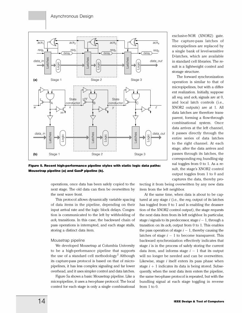
Figure 5a shows a basic Mousetrap pipeline. Like a

micropipeline, it uses a two-phase protocol. The local

control for each stage is only a single combinational

exclusive-NOR (XNOR2) gate.

The capture-pass latches of

micropipelines are replaced by

a single bank of level-sensitive

D-latches, which are available

in standard cell libraries. The re-

sult is a lightweight control and

storage structure.

The forward synchronization

operation is similar to that of

micropipelines, but with a differ-

ent realization. Initially, suppose

all reqi and acki signals are at 0,

and local latch controls (i.e.,

XNOR2 outputs) are at 1. All

data latches are therefore trans-

parent, forming a flow-through

combinational system. Once

data arrives at the left channel,

it passes directly through the

entire series of data latches

to the right channel. At each

stage, after the data arrives and

passes through its latches, the

corresponding reqi bundling sig-

nal toggles from 0 to 1. As a re-

sult, the stage’s XNOR2 control

output toggles from 1 to 0 and

captures the data, thereby pro-

tecting it from being overwritten by any new data

item from the left neighbor.

At the same time, when data is about to be cap-

tured at any stage i (i.e., the reqi output of its latches

has toggled from 0 to 1 and is enabling the deasser-

tion of the XNOR2 control output), the stage requests

the next data item from its left neighbor. In particular,

stage i signals to its predecessor, stage i ! 1, through a

transition on its acki output from 0 to 1. This enables

the pass operation of stage i ! 1, thereby causing the

latches of stage i ! 1 to become transparent. This

backward synchronization effectively indicates that

stage i is in the process of safely storing the current

data item, and informs stage i ! 1 that its output

will no longer be needed and can be overwritten.

Likewise, stage i itself enters its pass phase when

stage i # 1 indicates its data is being stored. Subse-

quently, when the next data item enters the pipeline,

the same two-phase protocol is repeated, but with the

bundling signal at each stage toggling in reverse

from 1 to 0.

Asynchronous Design

Latc

hes

Logi

c

req1

ack2

req0

ack1

data_in

Stage 1(a)

(b)

delay

Latc

hes

Logi

c

req2

ack3

Stage 2

delay

Stage 3

Latc

hes

Logi

c

req3

ack4

delay

data_out

Latc

hes

Logi

c

Latc

hes

Logi

c

Stateconductor

Stateconductor

Latc

hes

Logi

c

Stage 2Stage 1 Stage 3

A B Cw x y z

xx

yy

data_in data_out

Figure 5. Recent high-performance pipeline styles with static logic data paths:

Mousetrap pipeline (a) and GasP pipeline (b).

14 IEEE Design & Test of Computers

[3B2-9] mdt2011050008.3d 5/9/011 11:54 Page 14

For correct operation, a simple one-sided hold-

time constraint is required: a stage must fully capture

its current data (i.e., all data latches become opaque)

before its predecessor has passed any new data to its

latch inputs. This constraint can always be satisfied by

adding sufficient delay to the backward acki output, if

necessary.2

Interestingly, unlike almost all synchronous designs

using single data latches, Mousetrap has no two-sided

timing constraints (e.g., no pulse mode, or short ver-

sus long path constraints). In addition, in congested

scenarios, every stage can hold a distinct data item,

thereby providing 100% storage capacity with only

single data latches separating adjacent stages.

GasP pipelineFinally, another approach, GasP, was developed at

Sun Research Laboratories.3 Like Mousetrap, GasP

uses single D-latches for the data path. However, the

pipeline control includes dynamic logic and custom

gates, along with careful path timing. Figure 5b

shows a basic GasP pipeline.

GasP has several interesting features. First, unlike

Mousetrap, the data latches are normally opaque,

and a pulse-based latch control protocol is used.

Second, each control channel between adjacent

stages consists of a single wire (indicated as a

state conductor in the figure) instead of the usual

pair of request and acknowledge wires. This

single-track wire channel passes communication in

both directions. Initially, the wire is deasserted

high. To initiate a communication, an active-low re-

quest is sent from left to right. To complete the com-

munication, an active-high acknowledgment is sent

from right to left. As a result, the channel returns to

its default high state. No more than one channel

driver, left or right, can be active at any time, and

the control circuit is locally timed to avoid transient

short circuits. This novel protocol eliminates the

need for two wires; it effectively multiplexes the re-

quest and acknowledge onto a single wire.

Hence, GasP effectively combines the benefits of

both two-phase and four-phase protocols. Like a

two-phase protocol, there is only one round-trip com-

munication through GasP’s single-track channel. How-

ever, as in a four-phase protocol, the channel always

returns to the same value whenever a transaction is

complete.

Despite the protocol differences, the forward

synchronization operation of this pipeline is

fundamentally the same as in the previous designs.

If the pipeline is empty, all single-track channels

(w, x, y, z) are initially deasserted high, and data-

latch enable signals are deasserted low. When a

left request arrives by asserting w low, this request

causes each successive single-track channel to be

driven active-low through the inverters and the

NAND gate in each GasP stage. The active-low tran-

sition on each NAND gate also causes the corre-

sponding data latch enable signal to be asserted

high, thereby driving the stage’s data latches to be-

come transparent. As an immediate result, signal

transitions on the two short local loops deassert

both inputs of each NAND2 gate low, thereby releas-

ing the single-track channels and deasserting low

the latch enable signals. The net result is that

each stage’s latch enable undergoes a short pulse,

allowing the data to propagate forward through

the pipeline stage. In the reverse synchronization

operation, backward acknowledgments are driven

high on each channel, which is thus reset to its ini-

tial value.

The circuit designs are highly optimized for low la-

tency (i.e. use low ‘‘logical effort’’), require balanced

control path delays, and must satisfy two-sided timing

constraints (i.e., short and long path requirements).

A more aggressive implementation has also been

proposed.3

Several variants with longer forward and reverse

latencies have also been introduced. In particular,

to accommodate longer-latency logic blocks, a de-

signer can insert pairs of inverters on the forward

path to delay the firing of the n-transistor. Similarly,

a designer can add pairs of inverters on the reverse

path to delay the firing of the p-transistor, thereby

slowing down the pipeline operation for improved

timing margins.

Dynamic logic pipelinesThe second class of asynchronous pipelines oper-

ate on dynamic logic data paths. All the approaches

reviewed here use a four-phase (RZ) protocol and

are latchless (i.e., no explicit storage elements are

needed between adjacent stages).

Trade-offs in using dynamic logicDynamic data paths are common in high-

performance digital systems. By eliminating com-

plex pull-up transistor networks, dynamic gates can

provide the benefits of reduced chip area and

15September/October 2011

[3B2-9] mdt2011050008.3d 5/9/011 11:54 Page 15

reduced switched capacitance, which in turn can

lead to higher speed and lower energy consump-

tion. However, dynamic logic also has its drawbacks:

greater design and validation effort, and less noise

immunity. Therefore, it is typically used only in

speed-critical parts of a design!!for example, in

ASICs and in arithmetic and logic units used

in high-speed microprocessors. However, recent in-

dustrial efforts continue to demonstrate the viability

and benefits of dynamic logic, even in modern

advanced VLSI processes. For instance, Intrinsity

(recently acquired by Apple) has developed a com-

plete general-purpose synchronous CAD design

flow based on domino logic, and used it to imple-

ment high-performance and low-power processor

cores, including an ARM Cortex-A8 processor in

45-nm technology.

For several reasons, dynamic logic is an espe-

cially good match for asynchronous pipelines. In

particular, in dynamic asynchronous systems, the

gate type is typically fully staticized domino,4-7,11,17

in which each dynamic gate output has an attached

primary inverter along with a weak feedback inver-

ter, forming a lightweight storage element. Such

gates have good immunity to the effects of leakage,

charge sharing, and noise. Moreover, DI-encoded

asynchronous data paths can gracefully accommo-

date delay variations introduced by uncertainty in

charge sharing and noise, because individual bits

can safely arrive with arbitrary skew. As a result, dy-

namic logic has been widely used in several recent

high-performance asynchronous commercial prod-

ucts, such as Ethernet switch chips from Fulcrum

Microsystems (currently 65 nm) and FPGAs from

Achronix Semiconductor (90-nm down to 22-nm

technologies).

Dynamic logic and

asynchronous pipelinesA unique feature of many

asynchronous dynamic pipe-

lines is that they are latchless.

Thus, with proper sequencing

of control operations, an asyn-

chronous pipeline can exploit

the implicit latching functional-

ity of dynamic gates and entirely

avoid explicit storage elements

between stages. Achieving simi-

lar latchless operation in a

synchronous implementation

typically would require using complex multiphase

clocking. This asynchronous feature provides the

benefits of reduced critical delays, smaller chip

area, and lower power consumption, thereby mini-

mizing some of the key overheads of fine-grained

pipelining.

Several asynchronous dynamic logic approaches

have been proposed.4,6,7,17,23,26,27 We will begin

by reviewing the PS0 pipeline style by Williams

and Horowitz,4 which is influential and an

important foundation for most later styles. The

‘‘Advanced Asynchronous Dynamic Pipeline Styles’’

sidebar highlights two recent higher-performance

approaches: a timing-robust style called the pre-

charge half-buffer (PCHB) by Lines,6 and our high-

capacity (HC) style,7 which provides high through-

put and high storage density.

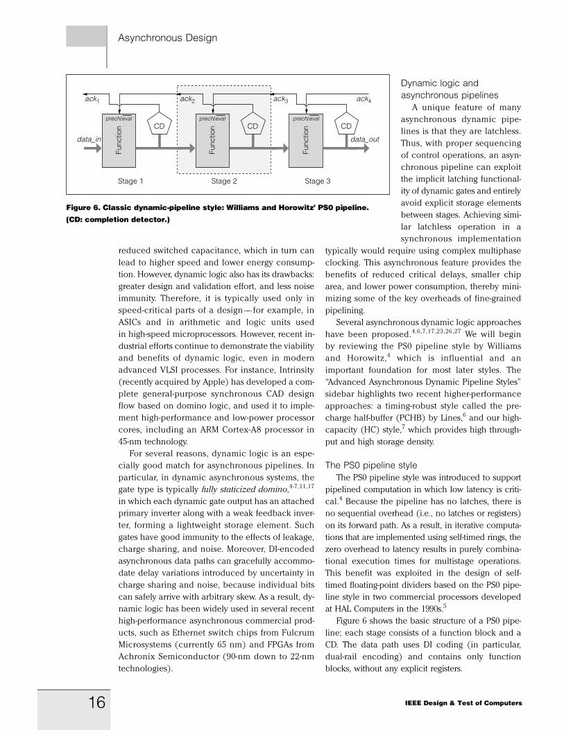
The PS0 pipeline style

The PS0 pipeline style was introduced to support

pipelined computation in which low latency is criti-

cal.4 Because the pipeline has no latches, there is

no sequential overhead (i.e., no latches or registers)

on its forward path. As a result, in iterative computa-

tions that are implemented using self-timed rings, the

zero overhead to latency results in purely combina-

tional execution times for multistage operations.

This benefit was exploited in the design of self-

timed floating-point dividers based on the PS0 pipe-

line style in two commercial processors developed

at HAL Computers in the 1990s.5

Figure 6 shows the basic structure of a PS0 pipe-

line; each stage consists of a function block and a

CD. The data path uses DI coding (in particular,

dual-rail encoding) and contains only function

blocks, without any explicit registers.

Asynchronous Design

Func

tion

prech/evalCD

ack1

Func

tion

prech/evalCD

ack2

Func

tion

prech/evalCD

ack3

Stage 2Stage 1 Stage 3

data_outdata_in

ack4

Figure 6. Classic dynamic-pipeline style: Williams and Horowitz’ PS0 pipeline.

(CD: completion detector.)

16 IEEE Design & Test of Computers

[3B2-9] mdt2011050008.3d 5/9/011 11:54 Page 16

Each function block alternates between an eval-

uate phase and a precharge phase. Initially, the func-

tion blocks have all 0 outputs, and hence are reset.

In the evaluate phase, the function is computed

after its data inputs arrive. In the precharge phase,

the function block is reset, with all its outputs

returning to 0. An important property of dynamic

logic in the precharge phase is that each stage has

an inherent blocking capability: new inputs applied

to its function are ignored by the dynamic block,

and the stage’s outputs remain reset. As a result,

evaluation and precharge of a dynamic function

block are somewhat analogous to making a latch

transparent and opaque, respectively, in static

logic pipelines.

A CD is attached to each stage’s output channel. In

each evaluate phase, the CD indicates when a com-

plete DI codeword has been generated (i.e., a func-

tion block’s computation is complete). In each

precharge phase, the CD indicates when a function

block’s outputs have all been reset to 0. The single

precharge-and-evaluate control input, prech=eval, of

a stage’s function block is connected from the output

of the next stage’s CD. A high value causes precharge,

and a low value enables evaluation. No latches are

needed between function blocks.

The coordination of pipeline control in a PS0 pipe-

line is quite simple, with two backward synchroniza-

tion events per cycle. These events follow two basic

rules: a stage is precharged whenever the next stage

finishes evaluation, and a stage evaluates whenever

the next stage finishes its precharge. This protocol

ensures that each pair of consecutive data tokens is

always separated by a reset token or spacer, in

which each dual-rail data bit in a stage is reset to a

00 value.

As an example, consider a simple simulation of

the PS0 pipeline operation. We can derive the com-

plete cycle of events for a PS0 pipeline stage by

observing how a single data item propagates after

arriving at the left input channel of an initially

empty three-stage pipeline. Initially, all pipeline

stages are in the evaluate phase, ready to receive

new data. After the data input arrives at stage 1,

there are three events from the start of the stage’s

evaluation phase to the start of its subsequent pre-

charge phase. First, stage 1 evaluates, and produces

a valid output. Second, stage 2 evaluates, and pro-

duces a valid output. Third, stage 2’s completion

detector detects completion of its evaluation.

Finally, stage 1 is enabled by the pipeline control

to enter its precharge phase.

Extending this simulation, we can trace the entire

cycle time of stage 1, from the start of its current eval-

uation phase, through its precharge phase, to the start

of its next evaluation phase. There are six successive

events:

1. Stage 1 evaluates.

2. Stage 2 evaluates.

3. Stage 3 evaluates.

4. The CD of stage 3 detects completion of evalua-

tion and initiates the precharge of stage 2.

5. Stage 2 precharges.

6. The CDof stage 2 detects completion of precharge,

thereby releasing the precharge of stage 1 and

enabling stage 1 to evaluate once again.

Thus, the cycle time of a pipeline stage is the sum of

the delays associated with these six events.

For a dual-rail code, a CD is implemented as

follows (details are available elsewhere4,5,9):

Each pair of rails, forming a bit, is the input to a

distinct OR2 gate, which evaluates if either rail

has been asserted high. The outputs of all such

OR2 gates are then combined together through a

tree of C-elements.1,4,8 Each C-element’s output is

asserted high when all its inputs are high, and

asserted low when all its inputs are low; otherwise,

it holds its current output value. Hence, the CD

asserts its output high when all bits have arrived,

and asserts its output low when all bits have

been reset.

The distributed nature of asynchronous control is

key to obtaining latchless operation in a PS0 pipe-

line. In particular, the pipeline style ensures that,

once stage 1 has completed evaluation, it will

hold its output stable as long as stage 2 is still

using the data of stage 1 (i.e., until stage 2 sends

stage 1 an acknowledgment). Thus, with this local

control sequencing, the dynamic function block it-

self implicitly provides the storage functionality

needed. In contrast, typical synchronous pipelines

employ a two-phase clock, which causes stage 1 to

start resetting while stage 2 starts evaluating. This

race condition in a synchronous pipeline requires

the insertion of a latch between the two function

blocks; alternatively, complex multiphase synchro-

nous clocking would be necessary to achieve simi-

lar effects.

17September/October 2011

[3B2-9] mdt2011050008.3d 5/9/011 11:54 Page 17

Asynchronous Design

Advanced Asynchronous Dynamic Pipeline StylesSeveral alternative dynamic pipeline styles have been

proposed specifically for achieving higher throughput.1-6

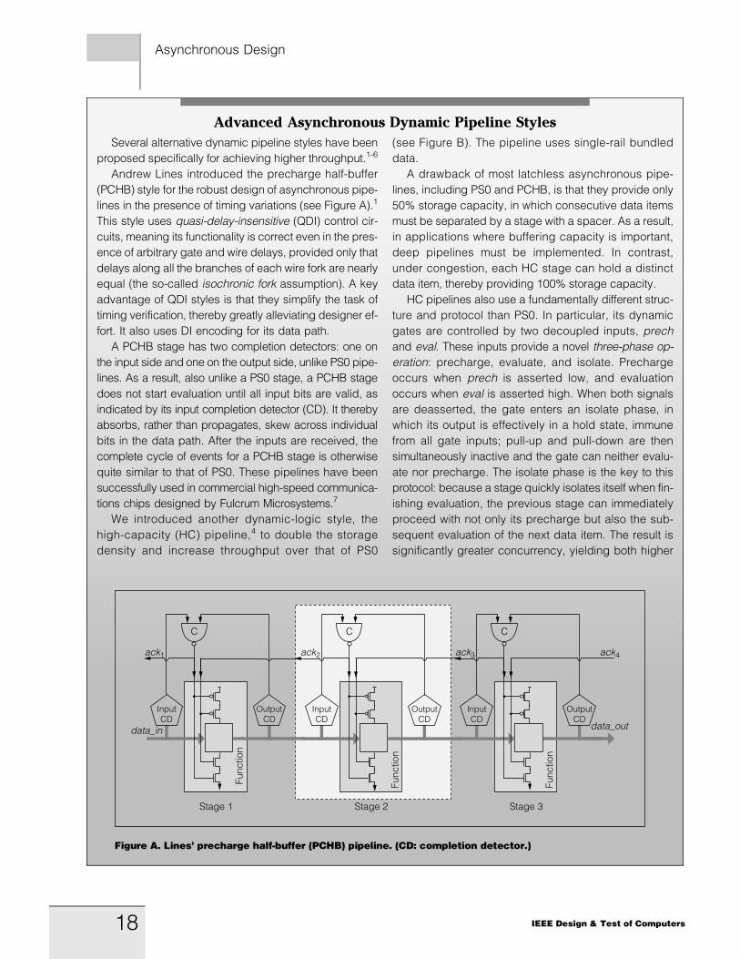
Andrew Lines introduced the precharge half-buffer

(PCHB) style for the robust design of asynchronous pipe-

lines in the presence of timing variations (see Figure A).1

This style uses quasi-delay-insensitive (QDI) control cir-

cuits, meaning its functionality is correct even in the pres-

ence of arbitrary gate and wire delays, provided only that

delays along all the branches of each wire fork are nearly

equal (the so-called isochronic fork assumption). A key

advantage of QDI styles is that they simplify the task of

timing verification, thereby greatly alleviating designer ef-

fort. It also uses DI encoding for its data path.

A PCHB stage has two completion detectors: one on

the input side and one on the output side, unlike PS0 pipe-

lines. As a result, also unlike a PS0 stage, a PCHB stage

does not start evaluation until all input bits are valid, as

indicated by its input completion detector (CD). It thereby

absorbs, rather than propagates, skew across individual

bits in the data path. After the inputs are received, the

complete cycle of events for a PCHB stage is otherwise

quite similar to that of PS0. These pipelines have been

successfully used in commercial high-speed communica-

tions chips designed by Fulcrum Microsystems.7

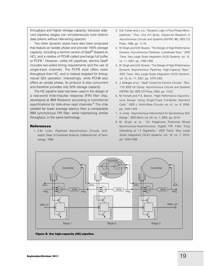
We introduced another dynamic-logic style, the

high-capacity (HC) pipeline,4 to double the storage

density and increase throughput over that of PS0

(see Figure B). The pipeline uses single-rail bundled

data.

A drawback of most latchless asynchronous pipe-

lines, including PS0 and PCHB, is that they provide only

50% storage capacity, in which consecutive data items

must be separated by a stage with a spacer. As a result,

in applications where buffering capacity is important,

deep pipelines must be implemented. In contrast,

under congestion, each HC stage can hold a distinct

data item, thereby providing 100% storage capacity.

HC pipelines also use a fundamentally different struc-

ture and protocol than PS0. In particular, its dynamic

gates are controlled by two decoupled inputs, prech

and eval. These inputs provide a novel three-phase op-

eration: precharge, evaluate, and isolate. Precharge

occurs when prech is asserted low, and evaluation

occurs when eval is asserted high. When both signals

are deasserted, the gate enters an isolate phase, in

which its output is effectively in a hold state, immune

from all gate inputs; pull-up and pull-down are then

simultaneously inactive and the gate can neither evalu-

ate nor precharge. The isolate phase is the key to this

protocol: because a stage quickly isolates itself when fin-

ishing evaluation, the previous stage can immediately

proceed with not only its precharge but also the sub-

sequent evaluation of the next data item. The result is

significantly greater concurrency, yielding both higher

Stage 2

OutputCD

ack2

C

InputCD

Func

tion

Stage 1

OutputCD

ack1

C

InputCD

data_in

Stage 3

OutputCD

ack3

C

InputCD

ack4

data_out

Func

tion

Func

tion

Figure A. Lines’ precharge half-buffer (PCHB) pipeline. (CD: completion detector.)

18 IEEE Design & Test of Computers

[3B2-9] mdt2011050008.3d 5/9/011 11:54 Page 18

throughput and higher storage capacity, because adja-

cent pipeline stages can simultaneously hold distinct

data tokens without intervening spacers.

Two other dynamic styles have also been proposed

that feature an isolate phase and provide 100% storage

capacity, including a domino version of GasP5 (based on

HC), and a relative of PCHB called precharge full buffer

or PCFB.1 However, unlike HC pipelines, domino GasP

includes two-sided timing requirements and the use of

single-track channels. The PCFB style offers lower

throughput than HC, and is instead targeted for timing-

robust QDI operation. Interestingly, while PCHB also

offers an isolate phase, its protocol is less concurrent

and therefore provides only 50% storage capacity.

The HC pipeline style has been used in the design of

a real-world finite-impulse response (FIR) filter chip,

developed at IBM Research according to commercial

specifications for disk-drive read channels.8 The chip

yielded far lower average latency than a comparable

IBM synchronous FIR filter, while maintaining similar

throughput, in the same technology.

References1. A.M. Lines, Pipelined Asynchronous Circuits, tech.

report, Dept. of Computer Science, California Inst. of Tech-

nology, 1998.

2. S.B. Furber and J. Liu, ‘‘Dynamic Logic in Four-Phase Micro-

pipelines,’’ Proc. 2nd Int’l Symp. Advanced Research in

Asynchronous Circuits and Systems (ASYNC 96), IEEE CS

Press, 1996, pp. 11-16.

3. M. Singh and S.M. Nowick, ‘‘The Design of High-Performance

Dynamic Asynchronous Pipelines: Lookahead Style,’’ IEEE

Trans. Very Large Scale Integration (VLSI) Systems, vol. 15,

no. 11, 2007, pp. 1256-1269.

4. M. Singh and S.M. Nowick, ‘‘The Design of High-Performance

Dynamic Asynchronous Pipelines: High-Capacity Style,’’

IEEE Trans. Very Large Scale Integration (VLSI) Systems,

vol. 15, no. 11, 2007, pp. 1270-1283.

5. J. Ebergen et al., ‘‘GasP Control for Domino Circuits,’’ Proc.

11th IEEE Int’l Symp. Asynchronous Circuits and Systems

(ASYNC 05), IEEE CS Press, 2005, pp. 12-22.

6. M. Ferretti and P.A. Beerel, ‘‘High Performance Asynchro-

nous Design Using Single-Track Full-Buffer Standard

Cells,’’ IEEE J. Solid-State Circuits, vol. 41, no. 6, 2006,

pp. 1444-1454.

7. A. Lines, ‘‘Asynchronous Interconnect for Synchronous SoC

Design,’’ IEEE Micro, vol. 24, no. 1, 2004, pp. 32-41.

8. M. Singh et al., ‘‘An Adaptively Pipelined Mixed

Synchronous-Asynchronous Digital FIR Filter Chip

Operating at 1.3 Gigahertz,’’ IEEE Trans. Very Large

Scale Integration (VLSI) Systems, vol. 18, no. 7, 2010,

pp. 1043-1056.

Stage 2

ack2

Func

tion

NAND

INV

aC+

gC+

_+

prec

h

eval

Controller

req2delay

req2req0

data_in

ack1

Func

tion

gC+

_+

prec

h

eval

Controller

Stage 1

delay

ack4

data_out

ack3

Func

tion

gC+

_+

prec

h

eval

req3

Stage 3

delay

Controller

Figure B. Our high-capacity (HC) pipeline.

19September/October 2011

[3B2-9] mdt2011050008.3d 5/9/011 11:54 Page 19

More recently, an alternative family of look-ahead

pipelines (LPs) provide optimizations that accelerate

the PS0 computation, and therefore increase through-

put, for both single-rail bundled and dual-rail data

paths.17

Choosing an asynchronouspipeline style

With many asynchronous pipeline styles avail-

able, a designer must consider several criteria to

choose an approach that is a good match for the in-

tended application. The choice of static versus dy-

namic data paths is typically determined by the

design tools and design effort available. In particu-

lar, static data paths are more amenable to synthesis

using standardized design tools and standard cell

libraries. Dynamic logic, on the other hand, requires

custom gates, as well as specialized design and

analysis tools for verifying timing and noise immu-

nity. On the whole, dynamic logic requires signifi-

cantly greater designer effort, although it can yield

somewhat higher performance. Similarly, single-rail

bundled-data design generally requires greater de-

sign and timing validation effort than DI encoding

to ensure bundling constraints are met, but it has

the benefits of smaller area, lower power, and

ease of reuse of synchronous function blocks. DI

encoding techniques can lead to 2 to 4 times as

much switching activity in the data path28!!although, recently, m-of-n22 and level-encoded

transition signaling (LETS)29 codes have been

shown to greatly reduce this gap. However, if

timing-robust operation in the presence of high vari-

ability is paramount, then using DI coding becomes

imperative, as the timing margins needed for safe

delay matching with single-rail bundled data be-

come unwieldy.

THE SIX PIPELINE STYLES reviewed in this article rep-

resent different trade-offs between performance,

power, and ease of design. Of the three static pipe-

lines, the GasP approach offers the highest perfor-

mance, although it involves significant design

effort because of its complex circuit structure and

operation, as well as its stringent timing constraints,

and is therefore more difficult to use with auto-

mated synthesis flows. The Mousetrap approach is

next in performance, and has the added benefit

of an entirely standard cell implementation; it

is therefore well-suited for automation. Of the

three dynamic pipelines, PS0 is the simplest to

implement, but it offers the lowest throughput.

The HC style has the highest throughput and

lowest energy consumption of the three, but it

requires matching of bundling delays. PCHB uses

quasi-delay-insensitive (QDI) control logic and DI

coding of the data path, and hence is highly robust

to variability.

Recent commercial and experimental chips

have validated the high performance of the asyn-

chronous pipeline styles reviewed in this article.

In particular, a test chip for a fine-grained pipelined

greatest common divisor (GCD) computation has

demonstrated Mousetrap pipelines capable of oper-

ating at 2.1 GHz in 130-nm technology.30 GasP pipe-

lines have demonstrated very high performance,

owing to their low-overhead protocol,3 including re-

cent results of 4 GHz in 90-nm technology for the

Infinity test chip at Sun Labs (now Oracle Labs).

Fulcrum Microsystems’ commercial Nexus crossbar

switch, operating at 1.35 GHz in 130-nm technol-

ogy,11 uses the PCHB pipeline style to implement

the data path.6 Finally, in an experimental, mixed-

synchronous/asynchronous FIR filter chip devel-

oped at IBM Research, operating at 1.8 GHz in

180-nm technology,12 the HC style is used to imple-

ment the speed-critical data path.7

Several support tools, design flows, extensions,

and applications for high-performance asynchronous

pipelines have been explored. These include system-

level performance analysis25 and optimization31,32

techniques, as well as some initial automated CAD

synthesis flows.24,27 Low-overhead testing techniques

have also been proposed.33,34 Recent pipelined appli-

cations include high-performance FPGA’s,10 Ethernet

switch chips,11 iterative dividers,4,5 FIR filters,12 and

NoCs.16,19

Synchronous methodologies that borrow from the

asynchronous design approach have also been pro-

posed,14,15 which adopt asynchronous ideas of back

pressure and handling of long global paths within

clocked systems. In addition, a desynchronization

methodology synthesizes asynchronous circuits from

a synchronous netlist by replacing the clock with

handshaking channels.35

Thus, there are exciting advances in the design,

optimization, tool support, and application of high-

speed asynchronous pipelines. There is also increas-

ing cross-fertilization with, and migration of asyn-

chrony into, the synchronous world.

Asynchronous Design

!

20 IEEE Design & Test of Computers

[3B2-9] mdt2011050008.3d 5/9/011 11:54 Page 20

AcknowledgmentsWe appreciate the funding support of the National

Science Foundation under grants CCF-0964606, CCF-

0811504, and CCF-0702712. We thank Jordi Cortadella

(Polytechnic University of Catalonia, Spain), Gennette

Gill (Columbia University), Andrew Lines (Fulcrum

Microsystems), Rajit Manohar (Cornell University),

Jens Sparsoe (Technical University of Denmark),

and Ivan Sutherland (Portland State University) for

their technical suggestions.

!References1. I.E. Sutherland, ‘‘Micropipelines,’’ Comm. ACM, vol. 32,

no. 6, 1989, pp. 720-738.

2. M. Singh and S.M. Nowick, ‘‘MOUSETRAP: High-Speed

Transition-Signaling Asynchronous Pipelines,’’ IEEE

Trans. Very Large Scale Integration (VLSI) Systems,

vol. 15, no. 6, 2007, pp. 684-698.

3. I. Sutherland and S. Fairbanks, ‘‘GasP: A Minimal

FIFO Control,’’ Proc. 7th Int’l Symp. Asynchronous

Circuits and Systems (ASYNC 01), IEEE CS Press,

2001, pp. 46-53.

4. T.E. Williams, ‘‘Self-Timed Rings and Their Application to

Division,’’ doctoral dissertation, Dept. of Electrical Eng.,

Stanford Univ., 1991.

5. T.E. Williams and M.A. Horowitz, ‘‘A Zero-Overhead Self-

Timed 160ns 54b CMOS Divider,’’ IEEE J. Solid-State

Circuits, vol. 26, no. 11, 1991, pp. 1651-1661.

6. A.M. Lines, Pipelined Asynchronous Circuits, tech. report

no. CaltechCSTR:1998.cs-tr-95-21, Dept. of Computer

Science, California Inst. of Technology, 1998.

7. M. Singh and S.M. Nowick, ‘‘The Design of High-

Performance Dynamic Asynchronous Pipelines: High-

Capacity Style,’’ IEEE Trans. Very Large Scale

Integration (VLSI) Systems, vol. 15, no. 11, 2007,

pp. 1270-1283.

8. D.E. Muller, ‘‘Asynchronous Logics and Application to

Information Processing,’’ Proc. Symp. the Application of

Switching Theory to Space Technology, Stanford Univer-

sity Press, 1963, pp. 289-297.

9. C.L. Seitz, ‘‘System Timing,’’ Introduction to VLSI Sys-

tems, C.A. Mead and L.A. Conway, eds., Addison-

Wesley, 1980, pp. 218-262.

10. C. La Frieda, B. Hill, and R. Manohar, ‘‘An Asynchronous

FPGA with Two-Phase Enable-Scaled Routing,’’ Proc.

IEEE Symp. Asynchronous Circuits and Systems

(ASYNC 10), IEEE CS Press, 2010, pp. 141-150.

11. A. Lines, ‘‘Asynchronous Interconnect for Synchronous

SoC Design,’’ IEEE Micro, vol. 24, no. 1, 2004,

pp. 32-41.

12. M. Singh et al., ‘‘An Adaptively Pipelined Mixed

Synchronous-Asynchronous Digital FIR Filter Chip

Operating at 1.3 Gigahertz,’’ IEEE Trans. Very Large

Scale Integration (VLSI) Systems, vol. 18, no. 7, 2010,

pp. 1043-1056.

13. S.M. Nowick et al., ‘‘Speculative Completion for the

Design of High-Performance Asynchronous Dynamic

Adders,’’ Proc. 3rd Int’l Symp. Advanced Research in

Asynchronous Circuits and Systems (ASYNC 97), IEEE

CS Press, 1997, pp. 210-223.

14. L.P. Carloni, K.L. McMillan, and A.L. Sangiovanni-

Vincentelli, ‘‘Theory of Latency-Insensitive Design,’’

IEEE Trans. Computer-Aided Design of Integrated

Circuits and Systems, vol. 20, no. 9, 2001,

pp. 1059-1076.

15. J. Carmona et al., ‘‘Elastic Circuits,’’ IEEE Trans.

Computer-Aided Design of Integrated Circuits and

Systems, vol. 28, no. 10, 2009, pp. 1437-1455.

16. M.N. Horak et al., ‘‘A Low-Overhead Asynchronous

Interconnection Network for GALS Chip Multiproces-

sors,’’ IEEE Trans. Computer-Aided Design of

Integrated Circuits and Systems, vol. 30, no. 4, 2011,

pp. 494-507.

17. M. Singh and S.M. Nowick, ‘‘The Design of High-

Performance Dynamic Asynchronous Pipelines: Look-

ahead Style,’’ IEEE Trans. Very Large Scale Integration

(VLSI) Systems, vol. 15, no. 11, 2007, pp. 1256-1269.

18. T. Chelcea and S.M. Nowick, ‘‘Robust Interfaces for

Mixed-Timing Systems,’’ IEEE Trans. Very Large Scale

Integration (VLSI) Systems, vol. 12, no. 8, 2004,

pp. 857-873.

19. E. Beigne et al., ‘‘An Asynchronous NOC Architecture

Providing Low Latency Service and Its Multi-level Design

Framework,’’ Proc. 11th IEEE Int’l Symp. Asynchronous

Circuits and Systems (ASYNC 05), IEEE CS Press,

2005, pp. 54-63.

20. A. Sheibanyrad, A. Greiner, and I. Miro-Panades, ‘‘Multi-

synchronous and Fully Asynchronous NoCs for GALS

Architectures,’’ IEEE Design & Test, vol. 25, no. 6, 2008,

pp. 572-580.

21. M. Choi et al., ‘‘Efficient and Robust Delay-Insensitive

QCA (Quantum-Dot Cellular Automata) Design,’’ Proc.

21st IEEE Int’l Symp. Defect and Fault-Tolerance in VLSI

Systems (DFT 06), IEEE CS Press, 2006, pp. 80-88.

22. W.J. Bainbridge et al., ‘‘Delay-Insensitive, Point-to-Point

Interconnect Using m-of-n Codes,’’ Proc. 9th Int’l Symp.

Asynchronous Circuits and Systems (ASYNC 03), IEEE

CS Press, 2003, pp. 132-140.

23. S.B. Furber and J. Liu, ‘‘Dynamic Logic in Four-Phase

Micropipelines,’’ Proc. 2nd Int’l Symp. Advanced

21September/October 2011

[3B2-9] mdt2011050008.3d 5/9/011 11:54 Page 21

Research in Asynchronous Circuits and Systems

(ASYNC 96), IEEE CS Press, 1996, pp. 11-16.

24. B. Quinton, M. Greenstreet, and S. Wilton, ‘‘Practical

Asynchronous Interconnect Network Design,’’ IEEE

Trans. Very Large Scale Integration (VLSI) Systems,

vol. 16, no. 5, 2008, pp. 579-588.

25. P.A. Beerel and A. Xie, ‘‘Performance Analysis of Asyn-

chronous Circuits Using Markov Chains,’’ Proc. Concur-

rency and Hardware Design, LNCS 2549, Springer,

2002, pp. 313-344.

26. J. Ebergen et al., ‘‘GasP Control for Domino Circuits,’’

Proc. 11th IEEE Int’l Symp. Asynchronous Circuits

and Systems (ASYNC 05), IEEE CS Press, 2005,

pp. 12-22.

27. M. Ferretti and P.A. Beerel, ‘‘High Performance Asyn-

chronous Design Using Single-Track Full-Buffer Standard

Cells,’’ IEEE J. Solid-State Circuits, vol. 41, no. 6, 2006,

pp. 1444-1454.

28. P.A. Beerel and M.E. Roncken, ‘‘Low Power and Energy

Efficient Asynchronous Design,’’ J. Low Power Electron-

ics, vol. 3, no. 3, 2007, pp. 234-253.

29. P.B. McGee et al., ‘‘A Level-Encoded Transition

Signaling Protocol for High-Throughput Asynchronous

Global Communication,’’ Proc. 14th IEEE Int’l Symp.

Asynchronous Circuits and Systems (ASYNC 08), IEEE

CS Press, 2008, pp. 116-127.

30. G. Gill et al., ‘‘A High-Speed GCD Chip: A Case Study

in Asynchronous Design,’’ Proc. IEEE Computer Society

Ann. Symp. VLSI, IEEE CS Press, 2009, pp. 205-210.

31. G. Gill and M. Singh, ‘‘Automated Microarchitectural Ex-

ploration for Achieving Throughput Targets in Pipelined

Asynchronous Systems,’’ Proc. IEEE Symp. Asynchro-

nous Circuits and Systems (ASYNC 10), IEEE CS

Press, 2010, pp. 117-127.

32. P. Prakash and A.J. Martin, ‘‘Slack Matching Quasi

Delay-Insensitive Circuits,’’ Proc. 12th IEEE Int’l Symp.

Asynchronous Circuits and Systems (ASYNC 06), IEEE

CS Press, 2006, pp. 195-204.

33. G. Gill et al., ‘‘Low-Overhead Testing of Delay Faults

in High-Speed Asynchronous Pipelines,’’ Proc. 12th

IEEE Int’l Symp. Asynchronous Circuits and Systems

(ASYNC 06), IEEE CS Press, 2006, pp. 46-56.

34. O.A. Petlin and S.B. Furber, ‘‘Scan Testing of Micropipe-

lines,’’ Proc. 13th IEEE VLSI Test Symp. (VTS 95), IEEE

CS Press, 1995, pp. 296-301.

35. J. Cortadella et al., ‘‘Desynchronization: Synthesis of

Asynchronous Circuits from Synchronous Specifica-

tions,’’ IEEE Trans. Computer-Aided Design of Inte-

grated Circuits and Systems, vol. 25, no. 10, 2006,

pp. 1904-1921.

Steven M. Nowick is a professor of computer

science and chair of the Computer Engineering Pro-

gram at Columbia University. His research interests

include the design and optimization of asynchronous

and mixed-timing circuits and systems; networks

on chips; low-power and high-performance digital

design; CAD tools for asynchronous systems; logic

synthesis; and encoding techniques for low-power,

delay-insensitive communication. He has a PhD in

computer science from Stanford University. He is a

Fellow of IEEE.

Montek Singh is an associate professor of computer

science at the University of North Carolina at Chapel

Hill. His research interests include asynchronous and

mixed-timing circuits and systems; CAD tools for de-

sign, analysis, and optimization; high-speed and low-

power VLSI design; and applications to emerging

computing technologies and energy-efficient graphics

hardware. He has a PhD in computer science from

Columbia University.

!Direct questions and comments about this article to

Steven M. Nowick, Dept. of Computer Science, Room

508, Computer Science Building, Columbia University,

New York, NY 10027; nowick@cs.columbia.edu; or

Montek Singh, Dept. of Computer Science, Sitterson

Hall Room FB234, University of North Carolina, Chapel

Hill, NC 27599; montek@cs.unc.edu.

Asynchronous Design

22 IEEE Design & Test of Computers

[3B2-9] mdt2011050008.3d 5/9/011 11:54 Page 22