High Precision Timing in Passive Measurements of Data Networksdjm202/pdf/papers/stephen-thesis.pdf · 2009-08-28 · High Precision Timing in Passive Measurements of Data Networks

High Precision Timing in Passive

Measurements of Data Networks

A thesis

submitted in partial fulfilment

of the requirements for the degree

of

Doctor of Philosophy

at the

University of Waikato

by

Stephen F Donnelly

Department of Computer Science

Hamilton, New Zealand

June 12, 2002

c 2002 Stephen F Donnelly

All Rights Reserved

ii

Abstract

Understanding, predicting, and improving network behaviour under a wide range of condi-

tions requires accurate models of protocols, network devices, and link properties. Accurate

models of the component parts comprising complex networks allows the plausible simula-

tion of networks in other configurations, or under differentloads. These models must be

constructed on a solid foundation of reliable and accurate data taken from measurements of

relevant facets of actual network behaviour.

As network link speeds increase, it is argued that traditional network measurement tech-

niques based primarily on software time-stamping and capture of packets will not scale to

the required performance levels. Problems examined include the difficulty of gaining ac-

cess to high speed network media to perform measurements, the insufficient resolution of

time-stamping clocks for capturing fine detail in packet arrival times, the lack of synchro-

nisation of clocks to global standards, the high and variable latency between packet arrival

and time-stamping, and the occurrence of packet loss withinthe measurement system. A

set of design requirements are developed to address these issues, especially in high-speed

network measurement systems.

A group at the University of Waikato including myself has developed a series of hardware

based passive network measurement systems called ‘Dags’. Dags use re-programmable

hardware and embedded processors to provide globally synchronised, low latency, reliable

time-stamping of all packet arrivals on high-speed networklinks with sub-hundred nanosec-

ond resolution. Packet loss within the measurement system is minimised by providing suf-

ficient bandwidth throughout for worst case loads and buffering to allow for contention over

shared resources. Any occurrence of packet loss despite these measures is reported, allow-

ing the invalidation of portions of the dataset if necessary. I was responsible for writing

iii

both the interactive monitor and network measurement code executed by the Dag’s embed-

ded processor, developing a Linux device driver including the software part of the ‘DUCK’

clock synchronisation system, and other ancillary software.

It is shown that the accuracy and reliability of the Dag measurement system allows confi-

dence that rare, unusual or unexpected features found in itsmeasurements are genuine and

do not simply reflect artifacts of the measurement equipment. With the use of a global clock

reference such as the Global Positioning System, synchronised multi-point passive measure-

ments can be made over large geographical distances. Both ofthese features are exploited

to perform calibration measurements of RIPE NCC’s Test Traffic Measurement System for

One-way-Delay over the Internet between New Zealand and theNetherlands. Accurate sin-

gle point passive measurement is used to determine error distributions in Round Trip Times

as measured by NLANR’s AMP project.

The high resolution afforded by the Dag measurement system also allows the examination

of the forwarding behaviour of individual network devices such as routers and firewalls at

fine time-scales. The effects of load, queueing parameters,and pauses in packet forward-

ing can be measured, along with the impact on the network traffic itself. This facility is

demonstrated by instrumenting routing equipment and a firewall which provide Internet

connectivity to the University of Auckland, providing passive measurements of forwarding

delay through the equipment.

iv

Acknowledgements

I would like to thank Ian Graham, my chief supervisor for his support, encouragement and

patience. Thanks go to John Cleary and Murray Pearson, members of my supervisory board

for their assistance and suggestions over the course of my work and in the preparation of this

thesis. Discussions on statistics with Ilze Ziedins were very useful, whom also kindly proof-

read early drafts of this thesis providing much needed feedback. Jed Martens designed and

debugged the Dag hardware and FPGA images, making much of this work possible. Thanks

go to Jorg Micheel and Klaus Mochalski for lengthy discussions on the analysis of various

datasets and their help with Dag software maintenance and tools. Henk Uijterwaal and

Rene Wilhelm provided access to RIPE NCC’s TTM system and measurements, assisted in

instrumenting the Amsterdam node and in analysing the results. Access to and assistance

with the collection of data from the NLANR AMP system was provided by Tony McGregor,

Matthew Luckie, and Jamie Curtis.

This work was partially supported by a University of WaikatoPostgraduate Scholarship.

The manuscript was typeset using LATEX.

v

vi

Contents

Abstract iii

Acknowledgements v

List of Figures xiii

List of Tables xv

List of Abbreviations and Units xvii

1 Introduction 1

2 An Overview of IP Network Measurement and Analysis 5

2.1 Passive Measurement . . . . . . . . . . . . . . . . . . . . . . . . . . . . . 5

2.2 Network Traffic Statistics Collection . . . . . . . . . . . . . . .. . . . . . 6

2.3 Packet Capture . . . . . . . . . . . . . . . . . . . . . . . . . . . . . . . . 7

2.3.1 Routers . . . . . . . . . . . . . . . . . . . . . . . . . . . . . . . . 8

2.3.2 Workstations . . . . . . . . . . . . . . . . . . . . . . . . . . . . . 8

2.3.3 Dedicated Measurement Equipment . . . . . . . . . . . . . . . . .11

2.4 Flow Based Measurement . . . . . . . . . . . . . . . . . . . . . . . . . . . 12

3 Software Based Measurement 15

3.1 Passive Measurement . . . . . . . . . . . . . . . . . . . . . . . . . . . . . 15

3.1.1 Interface Buffering and Queueing . . . . . . . . . . . . . . . . .. 17

3.1.2 Interrupt Latency . . . . . . . . . . . . . . . . . . . . . . . . . . . 18

3.2 Active Measurement . . . . . . . . . . . . . . . . . . . . . . . . . . . . . 22

3.2.1 Single-point Active Measurement . . . . . . . . . . . . . . . . .. 22

3.2.2 Multi-point Active Measurement . . . . . . . . . . . . . . . . . .. 23

vii

3.3 Passive Assisted Active Measurements . . . . . . . . . . . . . . .. . . . . 24

3.4 Clock Synchronisation . . . . . . . . . . . . . . . . . . . . . . . . . . . .25

4 Design Requirements for Accurate Passive Measurement 31

4.1 Media Access . . . . . . . . . . . . . . . . . . . . . . . . . . . . . . . . . 31

4.2 Time-stamping . . . . . . . . . . . . . . . . . . . . . . . . . . . . . . . . 33

4.2.1 Resolution . . . . . . . . . . . . . . . . . . . . . . . . . . . . . . 34

4.2.2 Latency . . . . . . . . . . . . . . . . . . . . . . . . . . . . . . . . 35

4.2.3 Wire Arrival and Exit Times . . . . . . . . . . . . . . . . . . . . . 35

4.3 Clock Synchronisation . . . . . . . . . . . . . . . . . . . . . . . . . . . .41

4.4 Packet Processing . . . . . . . . . . . . . . . . . . . . . . . . . . . . . . . 43

4.4.1 ATM: Segmentation and Re-assembly . . . . . . . . . . . . . . . .44

4.4.2 Filtering . . . . . . . . . . . . . . . . . . . . . . . . . . . . . . . . 45

4.4.3 CRCs: Integrity and Signatures . . . . . . . . . . . . . . . . . . .47

4.4.4 Data Reduction . . . . . . . . . . . . . . . . . . . . . . . . . . . . 49

4.5 System Integration . . . . . . . . . . . . . . . . . . . . . . . . . . . . . . 53

5 The Dag: A Hardware Based Measurement System 57

5.1 ATM-25 NIC . . . . . . . . . . . . . . . . . . . . . . . . . . . . . . . . . 58

5.2 OC-3c ATM NIC . . . . . . . . . . . . . . . . . . . . . . . . . . . . . . . 59

5.3 The Dag . . . . . . . . . . . . . . . . . . . . . . . . . . . . . . . . . . . . 61

5.4 The Dag 2 . . . . . . . . . . . . . . . . . . . . . . . . . . . . . . . . . . . 63

5.5 The Dag 3 . . . . . . . . . . . . . . . . . . . . . . . . . . . . . . . . . . . 66

5.5.1 Buffering . . . . . . . . . . . . . . . . . . . . . . . . . . . . . . . 67

5.5.2 IP Header Capture on ATM . . . . . . . . . . . . . . . . . . . . . 69

5.5.3 Time Formatting and Synchronisation . . . . . . . . . . . . . .. . 71

5.5.4 Packet over SONET . . . . . . . . . . . . . . . . . . . . . . . . . 82

5.5.5 Ethernet . . . . . . . . . . . . . . . . . . . . . . . . . . . . . . . . 86

5.5.6 The Dag 3.5 . . . . . . . . . . . . . . . . . . . . . . . . . . . . . . 89

5.5.7 Applications . . . . . . . . . . . . . . . . . . . . . . . . . . . . . 91

5.6 The Dag 4 . . . . . . . . . . . . . . . . . . . . . . . . . . . . . . . . . . . 92

5.7 Dag Software and Device Driver . . . . . . . . . . . . . . . . . . . . . .. 94

6 Passive Calibration of Active Measurement Systems 97

6.1 One-Way-Delay . . . . . . . . . . . . . . . . . . . . . . . . . . . . . . . . 97

viii

6.2 Test Traffic Measurement System . . . . . . . . . . . . . . . . . . . . .. 99

6.2.1 Calibration Methodology . . . . . . . . . . . . . . . . . . . . . . . 100

6.2.2 Transmission Latency . . . . . . . . . . . . . . . . . . . . . . . . 102

6.2.3 Transmission scheduling . . . . . . . . . . . . . . . . . . . . . . . 107

6.2.4 Reception Latency . . . . . . . . . . . . . . . . . . . . . . . . . . 110

6.2.5 End to End Comparison . . . . . . . . . . . . . . . . . . . . . . . 112

6.3 Instantaneous Packet Delay Variation . . . . . . . . . . . . . . .. . . . . . 117

6.4 Round Trip Time . . . . . . . . . . . . . . . . . . . . . . . . . . . . . . . 119

6.5 AMP: The Active Measurement Project . . . . . . . . . . . . . . . . .. . 122

6.5.1 Calibration Methodology . . . . . . . . . . . . . . . . . . . . . . . 122

6.5.2 RTT Error . . . . . . . . . . . . . . . . . . . . . . . . . . . . . . . 123

6.5.3 Target Response Time . . . . . . . . . . . . . . . . . . . . . . . . 130

6.6 Conclusions . . . . . . . . . . . . . . . . . . . . . . . . . . . . . . . . . . 131

7 Passive Characterisation of Network Equipment 135

7.1 Introduction . . . . . . . . . . . . . . . . . . . . . . . . . . . . . . . . . . 135

7.2 Device Characterisation . . . . . . . . . . . . . . . . . . . . . . . . . .. . 136

7.2.1 Active Method . . . . . . . . . . . . . . . . . . . . . . . . . . . . 136

7.2.2 Passive Method . . . . . . . . . . . . . . . . . . . . . . . . . . . . 137

7.2.3 Traffic Source . . . . . . . . . . . . . . . . . . . . . . . . . . . . . 138

7.2.4 Measurement System Requirements . . . . . . . . . . . . . . . . .138

7.2.5 Packet Delay and Loss Derivation . . . . . . . . . . . . . . . . . .139

7.2.6 Packet Recognition . . . . . . . . . . . . . . . . . . . . . . . . . . 140

7.2.7 IP Id as sequence number . . . . . . . . . . . . . . . . . . . . . . 140

7.2.8 Revised Passive Delay Derivation Algorithm . . . . . . . .. . . . 142

7.3 The University of Auckland Passive Measurements . . . . . .. . . . . . . 143

7.3.1 Measurement . . . . . . . . . . . . . . . . . . . . . . . . . . . . . 144

7.3.2 Link Characteristics . . . . . . . . . . . . . . . . . . . . . . . . . 145

7.3.3 Delay Datasets . . . . . . . . . . . . . . . . . . . . . . . . . . . . 147

7.3.4 Firewall Behaviour . . . . . . . . . . . . . . . . . . . . . . . . . . 149

7.3.5 Router/Switch Behaviour . . . . . . . . . . . . . . . . . . . . . . . 156

7.4 Conclusions . . . . . . . . . . . . . . . . . . . . . . . . . . . . . . . . . . 163

8 Conclusions and Future Work 165

ix

8.1 Conclusions . . . . . . . . . . . . . . . . . . . . . . . . . . . . . . . . . . 165

8.2 Future Work . . . . . . . . . . . . . . . . . . . . . . . . . . . . . . . . . . 167

Appendices

A ATM Partial SAR ARM Code 169

B AMP Monitors 179

Bibliography 183

x

List of Figures

3.1 Interrupt Latency Experimental Configuration . . . . . . . .. . . . . . . . 18

3.2 Interrupt Latency, Machine A. . . . . . . . . . . . . . . . . . . . . . .. . 20

3.3 Interrupt Latency, Machine B. . . . . . . . . . . . . . . . . . . . . . .. . 20

3.4 NTP Performance Experiment . . . . . . . . . . . . . . . . . . . . . . . .26

3.5 NTPv4 performance over LAN (Free-BSD 3.4) . . . . . . . . . . . .. . . 27

3.6 NTP Stratum 1 Performance Experiment . . . . . . . . . . . . . . . .. . . 28

3.7 NTPv4 Stratum 1 performance (Free-BSD 3.4) . . . . . . . . . . .. . . . 28

4.1 SONET Frame Structure . . . . . . . . . . . . . . . . . . . . . . . . . . . 37

4.2 Time-stamped Packet Flow . . . . . . . . . . . . . . . . . . . . . . . . . .39

4.3 BPF filter to accept all IP packets . . . . . . . . . . . . . . . . . . . .. . . 46

4.4 IP Packet Length Distribution . . . . . . . . . . . . . . . . . . . . . .. . . 50

4.5 Average IP Packet Size Per Minute . . . . . . . . . . . . . . . . . . . .. . 51

4.6 Header Length Distribution . . . . . . . . . . . . . . . . . . . . . . . .. . 52

5.1 ATM Ltd VL-2000 NIC and OC-3c Daughter-card Block Diagram . . . . . 60

5.2 Dag 1 Daughter card Block Diagram . . . . . . . . . . . . . . . . . . . .. 62

5.3 Dag 2.11 Block Diagram . . . . . . . . . . . . . . . . . . . . . . . . . . . 64

5.4 Dag 3.21 Block Diagram . . . . . . . . . . . . . . . . . . . . . . . . . . . 68

5.5 ATM Header and State Table Entry layout . . . . . . . . . . . . . . .. . . 70

5.6 Dag Time-stamp Format . . . . . . . . . . . . . . . . . . . . . . . . . . . 72

5.7 Dag 3 DUCK Clock Generator . . . . . . . . . . . . . . . . . . . . . . . . 75

5.8 Dag 3 Clock Waveform Comparison . . . . . . . . . . . . . . . . . . . . .76

5.9 24 Hour Crystal Oscillator Drift . . . . . . . . . . . . . . . . . . . .. . . 78

5.10 24 Hour DUCK Offset Error Distribution . . . . . . . . . . . . . .. . . . 78

5.11 Time-stamp Difference Experiment . . . . . . . . . . . . . . . . .. . . . 79

xi

5.12 Single Second Two-Dag Time-stamp Differences Histogram . . . . . . . . 80

5.13 24 Hour Two-Dag Time-stamp Differences Histogram . . . .. . . . . . . 81

5.14 24 Hour Two-Dag Time-stamp Differences Histogram, GPSvs CDMA . . . 82

5.15 IP Packet Length Distribution . . . . . . . . . . . . . . . . . . . . .. . . . 84

5.16 ATM Packet Length Distribution . . . . . . . . . . . . . . . . . . . .. . . 84

5.17 POS OC-3c Timing Error on Dag 3.21 . . . . . . . . . . . . . . . . . . .. 86

5.18 Dag 3.21E Block Diagram . . . . . . . . . . . . . . . . . . . . . . . . . . 87

5.19 Resistive Ethernet Tap . . . . . . . . . . . . . . . . . . . . . . . . . . .. 88

5.20 Dag 3.5 Block Diagram . . . . . . . . . . . . . . . . . . . . . . . . . . . . 89

5.21 Dag 4.1 Block Diagram . . . . . . . . . . . . . . . . . . . . . . . . . . . . 92

6.1 RIPE NCC Test Traffic Measurement System . . . . . . . . . . . . . .. . 99

6.2 Packet Transmission Time-line . . . . . . . . . . . . . . . . . . . . .. . . 103

6.3 TTM Transmission Latency Time-series . . . . . . . . . . . . . . .. . . . 104

6.4 TTM Transmission Latency Distribution . . . . . . . . . . . . . .. . . . . 104

6.5 TT01 Transmission Latency QQ plot . . . . . . . . . . . . . . . . . . .. . 105

6.6 TT47 Transmission Latency QQ plot . . . . . . . . . . . . . . . . . . .. . 106

6.7 TTM Transmission Latency Cumulative Distribution . . . .. . . . . . . . 107

6.8 TTM Inter-probe Spacing Time-series . . . . . . . . . . . . . . . .. . . . 108

6.9 TT01 Inter-probe Spacing Distribution . . . . . . . . . . . . . .. . . . . . 109

6.10 TT47 Inter-probe Spacing Distribution . . . . . . . . . . . . .. . . . . . . 109

6.11 Packet Reception Time-line . . . . . . . . . . . . . . . . . . . . . . .. . . 111

6.12 TTM Reception Latency Time-series . . . . . . . . . . . . . . . . .. . . . 113

6.13 TTM Reception Latency Distribution . . . . . . . . . . . . . . . .. . . . . 113

6.14 TTM Reception Latency Cumulative Distribution . . . . . .. . . . . . . . 115

6.15 TTM Type-P-One-way-Delay measured by Dag cards . . . . . .. . . . . . 115

6.16 TTM Total (Tx+Rx) Latency Time-series . . . . . . . . . . . . . .. . . . 116

6.17 TTM Total (Tx+Rx) Latency Distribution . . . . . . . . . . . . .. . . . . 116

6.18 Dag measured IPDV Cumulative Histogram . . . . . . . . . . . . .. . . . 118

6.19 Dag measured TT01–TT47 IPDV Histogram (200�s bins) . . . . . . . . . 120

6.20 Dag measured TT47–TT01 IPDV Histogram (200�s bins) . . . . . . . . . 120

6.21 Dag vs TTM IPDV Cumulative Histogram Comparison . . . . . .. . . . . 121

6.22 AMP Calibration Experiment . . . . . . . . . . . . . . . . . . . . . . .. . 123

6.23 AMP RTT Error Distribution for Un-modified ICMP . . . . . . .. . . . . 125

xii

6.24 AMP RTT Error Distribution for Modified IPMP . . . . . . . . . .. . . . 126

6.25 AMP RTT Error vs. RTT for Modified IPMP . . . . . . . . . . . . . . . .127

6.26 AMP RTT Error vs. Transmit Time for Modified IPMP . . . . . . .. . . . 128

6.27 AMP RTT Errors vs. Transmit Time for Modified IPMP (RTT 200–250ms) 128

6.28 Estimated AMP Host Clock Rate over One Second . . . . . . . . .. . . . 129

6.29 AMP ICMP Response Time Distribution . . . . . . . . . . . . . . . .. . . 132

6.30 AMP IPMP Response Time Distribution . . . . . . . . . . . . . . . .. . . 132

7.1 Active Device Characterisation . . . . . . . . . . . . . . . . . . . .. . . . 136

7.2 Passive Device Characterisation . . . . . . . . . . . . . . . . . . .. . . . 137

7.3 University of Auckland DMZ Instrumentation . . . . . . . . . .. . . . . . 143

7.4 Link Data Rates 00:01:00 to 00:02:00 . . . . . . . . . . . . . . . . .. . . 146

7.5 Link Data Rates 12:01:00 to 12:02:00 . . . . . . . . . . . . . . . . .. . . 146

7.6 Instantaneous Bandwidth CDF 00:01:00 to 00:02:00 . . . . .. . . . . . . 148

7.7 Instantaneous Bandwidth CDF 12:01:00 to 12:02:00 . . . . .. . . . . . . 148

7.8 Packet Delays dmz-o to dmz-i 00:01:00 to 00:02:00 . . . . . .. . . . . . . 150

7.9 Packet Delays dmz-o to dmz-i 12:01:00 to 12:02:00 . . . . . .. . . . . . . 150

7.10 Packet Delay Distribution dmz-o to dmz-i . . . . . . . . . . . .. . . . . . 153

7.11 Packet Delay vs. Size dmz-o to dmz-i . . . . . . . . . . . . . . . . .. . . 153

7.12 Packet Delay Sequence dmz-o to dmz-i . . . . . . . . . . . . . . . .. . . 154

7.13 Normalised Packet Delay vs. Size dmz-o to dmz-i . . . . . . .. . . . . . . 157

7.14 Normalised Packet Delay Histogram dmz-o to dmz-i . . . . .. . . . . . . 157

7.15 Packet Delays atm to dmz-o 00:01:00 to 00:02:00 . . . . . . .. . . . . . . 158

7.16 Packet Delays atm to dmz-o 12:01:00 to 12:02:00 . . . . . . .. . . . . . . 159

7.17 Packet Delay Distribution atm to dmz-o . . . . . . . . . . . . . .. . . . . 160

7.18 Low Packet Delay Distribution atm to dmz-o . . . . . . . . . . .. . . . . 160

7.19 Packet Delay vs. Size atm to dmz-o . . . . . . . . . . . . . . . . . . .. . 162

7.20 Normalised Packet Delay vs. Size atm to dmz-o . . . . . . . . .. . . . . . 162

7.21 Normalised Packet Delay Histogram atm to dmz-o . . . . . . .. . . . . . 163

xiii

xiv

List of Tables

3.1 Machines used for interrupt latency experiment. . . . . . .. . . . . . . . . 19

4.1 Time-stamp Clock Resolutions . . . . . . . . . . . . . . . . . . . . . .. . 35

4.2 SONET Row Overheads . . . . . . . . . . . . . . . . . . . . . . . . . . . 37

4.3 Typical Crystal Oscillator Frequency Error . . . . . . . . . .. . . . . . . . 41

4.4 PC Bus Theoretical Bandwidths . . . . . . . . . . . . . . . . . . . . . .. 54

6.1 TTM hosts used in calibration experiment. . . . . . . . . . . . .. . . . . . 100

6.2 TTM End to End Probe Experiment . . . . . . . . . . . . . . . . . . . . . 115

6.3 TTM Error Distribution . . . . . . . . . . . . . . . . . . . . . . . . . . . .117

6.4 Dag Measured IPDV Distribution . . . . . . . . . . . . . . . . . . . . .. 118

7.1 Summary of selected packet traces . . . . . . . . . . . . . . . . . . .. . . 145

7.2 Summary of IP Packet Delay Datasets . . . . . . . . . . . . . . . . . .. . 149

7.3 Summary of Selected IP Packet Delays . . . . . . . . . . . . . . . . .. . . 154

xv

xvi

List of Abbreviations and Units

Abbreviations

AAL ATM Adaption Layer

ALU Arithmetic Logic Unit

AS Autonomous System

ASIC Application Specific Integrated Circuit

ATM Asynchronous Transfer Mode

AWG American Wire Gauge

BCD Binary Coded Decimal

BPF BSD Packet Filter

CAM Content Addressable Memory

CAIDA Cooperatve Association for Internet Data Analysis

CDMA Code Division Multiple Access

CLP Cell Loss Priority

CPU Central Processing Unit

CS Convergence Sublayer

CSPF CMU/Stanford Packet Filter

DDS Direct Digital Synthesiser

DIX Digital Intel Xerox

xvii

DLPI Data Link Provider Interface

DMA Direct Master Access

DMZ De-Militarised Zone

DPT Dynamic Packet Transport

DUCK Dag Universal Clock Kit

FIFO First In First Out

FIQ Fast Interrupt Request

FPGA Field Programmable Gate Array

GFC Generic Flow Control

GPS Global Positioning System

HDLC High Level Data Link Control

HPC High Performance Connection

ICMP Internet Control Message Protocol

IFG Inter-Frame Gap

IPDV Instantaneous Packet Delay Variation

LAN Local Area Network

MAC Media Access Controller

MIB Management Information Base

MIPS Million Instructions Per Second

MOAT Measurement Operations and Analysis Team

MPF Mach Packet Filter

MRTG Multi Router Traffic Grapher

NIC Network Interface Card

NLANR National Laboratory for Applied Network Research

xviii

NNI Network-Network Interface

NSF National Science Foundation

NSS Nodal Switching Subsystem

OS Operating System

PCI Peripheral Component Interconnect

PCS Physical Coding Sublayer

PIO Programmed Input Output

PLL Phase Locked Loop

POINT PCI Optical Interface Network Transceiver

PME Packet Matching Engine

POH Path Overhead

POS Packet over SONET

PPS Pulse Per Second

PVC Permanent Virtual Circuits

RTFM Realtime Traffic Flow Measurement

RTT Round Trip Time

SAR Segmentation and Reassembly

SDH Synchronous Digital Hierarchy

SFD Start of Frame Delimiter

SNMP Simple Network Management Protocol

SONET Synchronous Optical Network

SRL Simple Ruleset Language

SVC Switched Virtual Circuits

TOH Transport Overhead

xix

TTL Time To Live

LPF Linux Packet Filter

RISC Reduced Instruction Set Computer

TTM Test Traffic Measurements

UNI User-Network Interface

vBNS Very High Speed Backbone Network Service

VC Virtual Circuit

VCI Virtual Circuit Identifier

VHDL VHSIC Hardware Description Language

VHSIC Very High Speed Integrated Circuit

VP Virtual Path

VPI Virtual Path Identifier

WAN Wide Area Network

WAND Waikato Applied Network Dynamics

WITS Waikato Internet Trace Storage

Units

b Bit, 1 Bit

kb Kilobit, 103 Bits

Mb Megabit,106 Bits

Gb Gigabit,109 Bits

b/s Bits per second

kb/s Kilobits per second

Mb/s Megabits per second

xx

Gb/s Gigabits per second

B Byte, 8 Bits

kB Kilobyte, 210 Bytes, 1024 Bytes

MB Megabyte,220 Bytes, 1024 Kilobytes

GB Gigabyte,230 Bytes, 1024 Megabytes

B/s Bytes per second

kB/s Kilobytes per second

MB/s Megabytes per second

GB/s Gigabytes per secondps picosecond,10�12 secondsns nanosecond,10�9 seconds�s microsecond,10�6 secondsms millisecond,10�3 seconds

xxi

Chapter 1

Introduction

During the 1990s the bandwidth available from emerging high-speed network link technolo-

gies considerably exceeded the average performance of the Internet. High speed research

and education networks such as the Very High Speed Backbone Network Service (vBNS)

were built in order to connect universities and research institutions, allowing the sharing of

data at higher speeds than was possible using the commercialInternet as well as research

into possible new network applications requiring high bandwidth connections. It became

clear as these networks were commissioned that users did notalways experience the perfor-

mance expected, given the provided network speeds. There were a number of root causes

for this low performance, including the exact tuning of the protocols used for the high per-

formance links. In order to diagnose these kinds of problemsit was realised that it was

important to be able to accurately capture the behaviour of the packets on the high-speed

network links.

In order to improve network performance, it is necessary to understand how packets from

different hosts using different protocols interact on high-speed links and within network

equipment such as Internet routers. This requires good models of how Internet hosts, pro-

tocols, and equipment behave, based on accurate measurement of their operation. With

good models of the network components, particular network configurations can be simu-

lated using computers, allowing the performance of the network to be predicted. Changes

can then be made to individual parameters, allowing researchers to see what causes perfor-

mance limitations and how adjustments might be made in protocols or network equipment

to overcome them.

1

I believe that the best way to understand protocol and packetdynamics on network links is

to observe the packets themselves under various conditionson operational network links.

This can provide both an understanding of what constitutes actual network traffic ‘in the

wild’, as well as the opportunity to investigate how packet streams interact within physical

network equipment.

Passive network measurement is the best way to observe packets on a network, without

disturbing the nature or timing of the pre-existing packets. In order to discern how packets,

protocols, and network equipment interact, the most important feature of the traffic to record

is the precise time at which each packet is observed on the network. This can provide much

information on network interactions, as shown later in thisthesis.

In order to record timing information about packets, it is necessary to have a good under-

standing and definition of thearrival time of the packet, or the time at which the packet’s

presence on the network link is recorded. Active network measurement systems which in-

ject packets into the network by their nature record the timeof the added packets before

they are sent. Passive measurement systems in contrast can only record the time at which

a packet was actually present on the network, at the point that the passive measurement

system is connected. I believe this is a superior measure, asit is the only objective, inde-

pendent, repeatable, and comparable measure of the time at which the packet was present.

The objective of this thesis is investigating how best to obtain an accurate passive measure

of packet’s arrival times on a network link.

The first part of this thesis discusses existing network measurement methods and their limi-

tations. A set of design requirements are developed for passive measurement, and a system

intended to meet these requirements is described.

Chapter 2 provides a brief history of passive measurement tools and techniques, noting im-

portant developments and lines of research. Chapter 3 describes both active and passive

software based network measurement systems, classifying them into several groups. The

operating principles of each group of tools is described along with their intended use, and

factors affecting their accuracy are discussed. Chapter 4 develops a set of design require-

ments for passive measurement, focusing on providing accurate time-stamps for packets on

high speed links. Issues investigated include media access, time-stamp definitions, latency,

and required resolution, clock synchronisation to a globalreference, packet processing in-

2

cluding handling Asynchronous Transfer Mode (ATM), packetfiltering, integrity testing,

signature generation and data reduction, and systems integration including host require-

ments. Chapter 5 describes the series of passive measurement systems developed to meet

these requirements for various network media at the University of Waikato. Each system’s

important features and method of operation are described, along with its limitations and

practical performance. Possible applications are discussed, and published works using data

collected by each system are referenced.

The second part of this thesis presents some applications ofthe Dag measurement system.

Chapter 6 describes how the Dag hardware based passive measurement system can be used

to measure One-way-Delay over geographical distances. An application of this capability is

presented, independently measuring the wire arrival timesof One-way-Delay probe packets

from the RIPE Test Traffic Measurement system at both transmitter and receiver located at

the University of Waikato and at RIPE NCC in the Netherlands,in order to characterise the

system’s error. Latencies in the transmission and reception of probe packets are measured

and presented, along with the total difference in the measured One-way-Delays. Calibration

measurements are also made of NLANR MOAT’s AMP system for packet round trip time

measurements, using a single passive measurement system colocated with one of the AMP

monitors at the University of Waikato. The errors in round trip times as measured by both

the ICMP and IPMP protocols are described, and the time takenby a measurement target to

reply to an incoming request is also determined.

Chapter 7 describes how the Dag passive measurement system can be used to measure very

small packet delays. An experiment to non-intrusively measure the packet delay through a

firewall and some routing equipment carrying operational traffic at the University of Auck-

land is presented. The distribution of delays through the network equipment at different

times of day is analysed in depth and explained.

Conclusions are presented in chapter 8. In high-speed networks, flexible custom hardware

can provide accurate and reliable passive measurements at reasonable cost where software

based systems lack the necessary accuracy, resolution and repeatability due to the unsuit-

ability of generic NICs and software issues.

3

4

Chapter 2

An Overview of IP Network

Measurement and Analysis

2.1 Passive Measurement

As long as computers have been communicating there has been aneed to debug network

protocol stacks, device drivers, and network interfaces. As networks have become more

complex, consisting of more nodes, operating at higher datarates, and an increasingly het-

erogeneous mix of network devices and protocol implementations, the need to understand

both individual packet transactions on networks and the nature of their interactions has be-

come more important.

Simulation is an important tool in network research, allowing the behaviour of various net-

work configurations to be examined without having to actually construct them, which may

be expensive, or impossible if proposed mechanisms are being tested. The simulation envi-

ronment allows a variety of variables to be altered and compared inexpensively. In order for

simulations to be accurate and useful, good models of the equipment and networks being

simulated, the protocols in use, and realistic usage patterns are needed.

Passive network measurement is a method of observing packets on a data link or shared

network media without generating any additional traffic on that media which may disturb the

existing network behaviour. Packets may be observed by any device attached to the network

to be observed, including end hosts such as workstations, packet forwarding devices such

5

as routers, or special purpose measurement equipment.

When a packet is received from the network, the measuring host applies a time-stamp in

order to preserve a notion of the time-profile of the packet onthe network. The entire

packet, or a subsection of it such as the protocol headers, isthen optionally passed through

a filter that may select packets by such criteria as network address or protocol. The accepted

packets or packet records are then available for further analysis or storage as a packet trace

file for later use.

Passive network traces can be used to diagnose faults in the network, characterise the com-

ponent mix of an aggregated traffic stream, and observe trends in behaviour over long time

periods. Network traces are essential in the generation of models for protocols, applications,

and usage patterns.

If aggregated traffic is desired for a simulation, for instance to investigate different queueing

schemes in a router, then a large number of individual end hosts may be simulated acting as

clients and servers to generate a load on the router. It may not be feasible to simulate indi-

vidually each host for situations requiring a large amount of traffic however. Network traces

can be used to derive statistical models of aggregate trafficfor use in these simulations. In

some cases the recorded network trace may be used directly asinput to a simulation. This

trace-driven simulationapproach is immune to flaws in the models of the low level details

of the traffic sources and sinks, as actual network traffic is used. It is somewhat less flexi-

ble however, as the input to the simulation is not as tunable for simulation under different

network conditions as a synthetic model. Trace-driven simulation may also be unsuited to

simulations that investigate feedback mechanisms in protocols such as TCP that alter their

behaviour depending on network conditions.

2.2 Network Traffic Statistics Collection

This section provides a brief overview of the collection of basic traffic statistics from IP

networks.

Many network devices such as routers and managed switches are capable of recording at

least simple statistics such as packet and byte counts on a per interface basis. These fea-

6

tures, although limited, provide an important source of information to help understand the

network, as they are widely deployed. The IETF has standardised a set of these functions as

an Simple Network Management Protocol (SNMP) Management Information Base (MIB),

called MIB-II [McCloghrie and Rose, 1991]. This MIB is widely deployed in commercial

equipment, often with vendor specific extensions.

Network operators frequently collect link utilisation data available from compliant network

devices and use the Multi Router Traffic Grapher (MRTG) software package to automati-

cally graph the data. These graphs are then used to monitor link health in real-time, and as

a historical record for link sizing and capacity planning.

An early example of router based measurement was in the T1 based NSFNET [Claffy et al.,

1993b]. Evolving from a small network of 6 nodes linked by 56kb/s lines, the NSFNET

was upgraded to 1.544Mb/s T1 links in 1988, and to 45Mb/s T3 links in the early 1990s.

The T1-era NSFNET backbone routing was performed by a multiprocessor PC/RT based

device called the Nodal Switching Subsystem (NSS). Each NSStypically contained nine

processors arranged in an internal token ring with one processor dedicated to measurement,

running the NNStat package [Braden and DeSchon, 1998]. Thispackage provides packet

categorisation information, maintaining several statistical objects such as packet length,

protocol and TCP port distributions, and a source-destination AS matrix. These objects are

collected by a central agent every 15 minutes, with a total data volume up to 50MB daily.

During the 1990-91 period during the transition to T3 circuits it became clear by comparing

interface statistics from the NSS interfaces with the NNStat output that the processor run-

ning the NNStat package was unable to keep up with the data flow, and a sampling scheme

was deployed where only one in fifty packets were passed through NNStat. Investigation

into this sampling scheme showed that the distributions built from the captured sample were

statistically compatible with the original population forat least some metrics [Claffy et al.,

1993a].

2.3 Packet Capture

Packet capture can be accomplished by almost any device connected to a network segment:

workstations, servers, routers, or dedicated measurementequipment.

7

2.3.1 Routers

Routers may appear to be a desirable place at which to capturepackets as they may be con-

nected to more than one network. Unfortunately since their primary priority is forwarding

packets, these devices may not have excess CPU or backplane resources to perform packet

capture and filtering functions, and seldom contain mass storage devices. This means that

packet capture at a router must either be limited to a very small number of packet records,

to summary data about packets such as counts or histograms ofpacket inter-arrival times,

or the captured data must immediately be sent out of the router on another network to a

separate device for storage. Router interface cards may also not be capable of accurately

time-stamping packet arrivals as this functionality is notneeded for packet forwarding.

The IETF has standardised a SNMP access and control method for remote network monitors

in the RMON MIB, with proposed extensions in the RMON-II MIB [Waldbusser, 2000,

1997]. This provides a method for configuring packet filters in a remote network monitor

and causing the monitor to accumulate full or partial packetrecords in a table to be retrieved

later by SNMP. The MIB can be implemented by a stand-alone device or internally in a

router, but routers may have limited memory space in which tostore captured packets,

limiting the volume of packets that can be usefully collected.

2.3.2 Workstations

Workstation computers or PCs are readily available and relatively low cost, and typically

contain at least one Network Interface Card (NIC), connecting it to a Local Area Net-

work (LAN). Their low cost makes them the first choice for packet capture from their LAN

connections, but they may not have Wide Area Network (WAN) orhigh-speed interfaces

necessary to perform packet capture on some networks.

The LAN NIC in a workstation typically only delivers to the operating system packets with a

link layer destination address matching the NIC, but can be set to the so calledpromiscuous

modewhere they present all valid received packets to the operating system regardless of

destination address. On shared network segments containing a large number of hosts, there

may be a large number of packets present on the network that are usually discarded by

the NIC. Activating promiscuous mode in such a situation maysignificantly increase the

8

interrupt and bus load of the host as the extra packets are delivered.

Once the packet has been transferred to a buffer in host memory, packet tap code in the

network stack makes the raw unprocessed packet available touser space programs via some

interface. Most workstation operating systems provide such a mechanism, such as NIT in

Sun’s SunOS [Sun, 1990], the Ultrix Packet Filter in DEC’s Ultrix, Snoop in SGI’s IRIX,

and the Packet Socket in the Linux kernel [Kleen, 1999].

Packet filtering

Transferring a packet into user space from a kernel packet capture facility usually requires

copying the packet in memory which can be expensive at high packet rates, especially since

often not all of the packets are desired. What was needed was away to select certain

packets to be sent to user space within the kernel. This problem was addressed by packet

filters, which are often an integral part of the packet capture system.

In 1980 the CMU/Stanford Packet Filter (CSPF) was developed[Mogul et al., 1987]. This

was designed to allow arbitrary filters to operate on received packets, typically performing

comparisons of packet header fields to determine whether to discard the packet or send it to

user space. The CSPF architecture was a boolean expression tree, and was implemented as

a virtual stack based machine, mapping naturally to stack based processors.

Packet filter design progressed in the 1980s, focusing on efficient implementation. In 1990

the BSD Packet Filter (BPF) was written, the best known packet filter [McCanne and Jacob-

son, 1993]. It used the directed acyclic control flow graph approach to filtering, mapping

naturally to a pseudo machine implementation on the register based Central Processing

Unit (CPU)s found in workstations. In some situations the BPF was much more efficient

than the boolean tree based filters, and had more scope for optimisation, leading to much

better performance.

With network data rates increasing during the 1990s work continued on refining packet

filters. The Mach Packet Filter (MPF) extended the BPF to efficiently support any number

of independent filters [Yuhara et al., 1994]. PathFinder used a pattern matching based virtual

machine with high performance that was amenable to hardwareimplementation [Bailey

et al., 1994]. The DPF enhanced PathFinder using dynamic code generation to exploit

9

runtime knowledge for greater performance [Engler and Kaashoek, 1996], and the BPF+

proposed a general packet filter framework that exploited global data-flow optimisations

[Begel et al., 1999].

These sophisticated packet filters allow multiple optimised packet filters to run on the same

host for each packet, reducing the number of packets that need to be sent to user space; but

in the case where all packets are desired, they provide no benefit.

Packet Recording

While all packet filters provide some user space interface tothe captured packets, their

interfaces are not standardised. This makes it difficult to build portable network analysis

programs, as they must be altered to work with different packet filters when they are ported

to a new platform. To enable portable network analysis code to be written,libpcap

was developed along with the BPF [McCanne et al., 1994]. Thislibrary can read packets

from many packet filters, including BPF, Data Link Provider Interface (DLPI), Enet, NIT

and SNIT, Packet Filter, Snoop, and Linux’s Packet Socket, presenting a common packet

capture API to user programs. Thelibpcap library allows the reading and writing of

sequences of captured packets to and from files, allowing thelong term storage of network

traces in a broadly supported format.

Although most kernel packet packet capture interfaces support filtering, libpcap only

uses in-kernel filtering for the BPF interface. On systems with other filters, all packets are

read from the kernel and the BPF filter is evaluated in user space, incurring the kernel to

user space penalty even for rejected packets.

Once the desired packets are in user space, vialibpcap or some other mechanism, they

may be analysed immediately or stored for later study or to create an archive of the network

over time. A multitude of software packages are available for this task, includingnetfind,

ethereal andtcpdump [McCanne et al., 1991]. Intcpdump, packets are read from

the kernel vialibpcap or from a file, filtered with the BPF, their headers can be displayed

in human readable form, and the filtered packets can be written to a file.

It is possible to specify asnaplenparameter which limits the number of bytes of the packet

read from the kernel or written to disk. This may be desirableas in many cases all of the

10

necessary information about the packet is contained in the packet protocol headers, and the

content of the packet is not needed. Since the size of IP packets can exceed 1500 bytes but

IP headers seldom exceed 40 bytes, this can greatly reduce the size of the recorded trace

file, and also reduce the bandwidth to the storage medium required to record the packet

stream as it arrives from the kernel. Insufficient storage bandwidth can cause packets to be

dropped, resulting in an incomplete packet trace file. With adefault snaplen of 68 bytes and

the average IP packet size typically several hundred bytes depending on the protocol mix,

the bandwidth savings by recording partial packets may be greater than 5:1.

2.3.3 Dedicated Measurement Equipment

There is a wide variety of commercial network test equipment, ranging from hand held line

testers to large protocol analysers, some of which has the capability to record packet traces.

Most network equipment is designed for online analysis, generating counts in real time

of link layer faults, or classifying and counting packets byprotocol. Not being designed

for recording long packet traces, these devices allow only asmall number of packets to be

captured into buffer memory for later study. High end equipment may have hundreds of

megabytes of capture memory, and incorporate complete userprogrammable UNIX hosts

with hard disk storage, accommodating the recording of the capture buffer to disk or transfer

to a workstation. Since these systems are not user expandable, they rarely have the high

speed disk systems necessary to record packet trace files from the network directly.

The primary advantage of dedicated network measurement andtest equipment is media ac-

cess. Frequently designed with modular network interfaces, test equipment can measure a

much greater variety of network types and media than are available as NICs for worksta-

tions, and in some cases may be the only way to capture packetsfrom an unusual network

link. Dedicated network measurement equipment often has the capability to generate high

resolution time-stamps for packets as they are received, before any buffering that would

contaminate the time-stamps. Such equipment must be reliable, and is designed so that it

will never lose a packet within its own data path due to bandwidth or buffer constraints,

guaranteeing that all packets from the network are faithfully recorded.

Test equipment generally uses a high resolution clock to generate its time-stamps, and this

clock is distributed to all of the interfaces on the device, allowing captures from multiple in-

11

terfaces with consistent time-stamps. The time source is usually a form of crystal oscillator,

which varies in frequency slightly with temperature and supply voltage. Without the ability

to use an external reference signal to correct for these variations it may not be possible to

compare packet traces recorded by different devices, especially if they are geographically

separated.

The main disadvantage of test equipment is its cost. Becauseit is a low volume product,

margins and hence prices are high. For fixed cost measurementprojects this may reduce the

availability of the equipment, or the scope of the project with fewer measurements possible

simultaneously due to the lower number of measurement systems. Diagnostic test equip-

ment is also typically designed to be used interactively by an engineer or technician. This

may make it unsuitable for long term installation in a network centre, if the remote operating

facilities are limited.

2.4 Flow Based Measurement

Flow based measurement describes a number of approaches to network measurement at a

higher level than individual packets. Rather than collecting statistics like packet counts on

a per interface basis or recording headers from all packets,flow based measurement cat-

egorises packets into higher level objects calledflowsbased on some criteria and reports

statistics only on these objects. The flow is timed out when nomatching packets are ob-

served for some preset period [Jain and Routhier, 1986; Acharya et al., 1992; Acharya and

Bhalla, 1994].

As well as the flow timeout parameter, several other factors define a flow specification:

directionality, endpoint count, endpoint granularity, and functional layer [Claffy, 1994].

Flows can be either unidirectional, and may be measured on a single unidirectional network

media, or bidirectional, which may require two network monitors on separate unidirectional

network media. If packets must be collected from two monitors, merging the two packet

record streams to create bidirectional flows may be expensive at high packet rates. Flows

may be defined using only their source attributes, only theirdestination attributes, or both.

The granularity of the communicating entities forming the flow can be of several scales,

including by application, end user, host, IP network number, Autonomous System (AS),

12

backbone node interface, backbone node, backbone, or arbitrary environment such as coun-

try. Flows can be defined at different functional or protocollayers, such as the application,

transport, or even link layer such as an ATM virtual circuit.

Flow based measurement requires a stream of packets or packet headers, either from a live

measurement session on a network link, or from a packet tracefile recorded earlier. An

example istcptrace which can read live packets from the kernel using pcap or parse

several packet trace file formats to produce flow informationfor all TCP flows observed, or

produce several types of graphical plots of individual flows.

OC3MON was developed from 1995 by MCI as an inexpensive system to perform unidi-

rectional IP flow measurements on ATM OC-3c links principally for the vBNS [Apisdorf

et al., 1994]. Hosted on a commodity PC running MS-DOS, the OC3MON software used a

FORE Systems ATM NIC with custom firmware to capture the first cell from each packet.

Software on the PC then performed flows analysis from these cells in real-time, recording

results to disk.

The NICs used were not designed for network measurement, andthe hardware for generat-

ing time-stamps had no capability for external synchronisation, and had complicated over-

flow behaviour requiring post processing to correct. The useof MS-DOS as the operating

system ensured that the OC3MON software had complete control of the computer avoiding

scheduling problems on the relatively slow computers of theday, but made remote access

and control of the monitor more difficult. This, together with reliance on inefficient block-

ing BIOS calls for disk access and the lack of DOS support for newer network hardware,

made a port to a more capable UNIX host desirable.

A port of OC3MON to FreeBSD, Coral, was done by NLANR. This used the same hardware

and firmware as the DOS OC3MON, but the capturing software ranon the UNIX host. The

vBNS upgraded its backbone from OC-3c to OC-12c links, and a network monitor for the

higher speed links was needed. MCI and NLANR commissioned Applied Telecom Inc to

design and build a passive network monitoring card to support OC12mon, called the PCI

Optical Interface Network Transceiver (POINT) card which was also supported by the Coral

software [Apptel, 1999].

CoralReef is the evolutionary successor to Coral [Keys et al., 2001]. Developed by CAIDA,

13

CoralReef has expanded into a comprehensive suite for collecting and analysing data from

passive network monitors, including extensive user APIs inC and Perl. Packets can be

read from a variety of file formats, livelibpcap interfaces, FORE Systems OC-3c NICs,

Apptel POINT OC-3c and OC-12c ATM cards, and Dag cards for OC-3c and OC-12c ATM

as well as OC-3c, OC-12c, and OC-48c POS (see chapter 5).

An IETF working group has defined an architecture for real-time traffic flow measurement

and reporting, called the Realtime Traffic Flow Measurement(RTFM) [Brownlee et al.,

1999]. The first implementation of this standard is called NeTraMet, and was originally im-

plemented on IBM compatible PCs running MS-DOS using DOS packet drivers for packet

acquisition [Brownlee, 1999a]. It has now been ported to UNIX with alibpcap interface,

and can also accept packet records from a CoralReef monitor or a Dag card based monitor.

Some routers maintain internal state for each flow to speed packet forwarding or avoid

performing costly operations such as routing or access control lookups for each packet in

a flow individually. In some equipment this information can be extracted, providing some

flow measurement capability. This may be very convenient as such equipment is often

already in place and well placed to monitor highly aggregated backbone links.

Cisco’s NetFlow is an example of such a vendor specific system[Cisco, 2000]. Cisco

routers can maintain a local unidirectional flow cache of up to 128k entries depending on

the model. As flow entries are removed from the cache, their summary information can be

placed into a NetFlow Export UDP packet and sent to a flow collector. Each UDP frame

can contain information for up to 30 flows, such as source and destination address, ports

and AS, protocol, type of service, start and end time-stamps, and even the address of the

next hop router. NetFlow and NetFlow export can place a heavyload on the router however,

which may lead to the loss of some flow records or an impact on packet forwarding. Cisco

warns ‘NetFlow services should be utilised as an edge metering and access list performance

acceleration tool and not activated on “hot” core/backbonerouters or routers running at

very high CPU utilisation rates’. This unfortunately may bethe very location where flow

measurements would be most useful, potentially limiting the utility of NetFlow Export for

network research.

14

Chapter 3

Software Based Measurement

When a program of network research is begun, the first tools generally employed are soft-

ware based. Many of these tools (eg.ping, traceroute, tcpdump) are widely

available on workstation or desktop computers that researchers also use for other tasks.

These tools provide a simple way to investigate a LAN, or perform experiments across the

Internet without having to purchase any additional equipment.

In this chapter I will investigate the performance and limitations of these methods, in order

to build a comparison with alternative methods.

3.1 Passive Measurement

Passive network measurement is the process of examining thetraffic on a network at one

or more points, without introducing packets onto the network, or otherwise disturbing it in

any way. Many different aspects of the network, its traffic, and behaviour can be studied in

this way. Simply monitoring the numbers of packets and theirsize on a network link can

provide useful operational information on link utilisation, that can further be used for route

planning, and network provisioning.

If the headers of the packets are captured for analysis, protocol information can be collected

for a wide number of purposes. They can be used to debug network protocols, and anal-

yse network stacks for conformance or to investigate behaviour under various real network

conditions. In the case of IP, the application mix of the traffic can be discovered for known

15

ports, which can be used to observe trends and changes in traffic patterns. This informa-

tion may be useful in predicting future traffic patterns or modelling application mixes for

simulation.

If accurate time-stamps can be recorded for packets as they pass the measurement station,

the time or arrival characteristics of the traffic can be analysed for long range dependence,

or fractal structure.

If protocol header information is collected along with accurate time-stamps, then the time

behaviour of different protocols can be investigated, and the temporal structure of individual

end to end connection sessions can be analysed, even estimating the performance that the

connection is achieving, or estimating the delays to and from the connection endpoints from

the measurement point.

The ideal passive measurement system then, is one that collects for each packet an accurate

time-stamp, and from the contents of the packet at least the protocol headers. It is possible

to collect the packet payloads also, but this is often discouraged due to privacy concerns,

since the majority of data on networks today is not encrypted. Collecting entire packets can

be useful in some debugging situations, but also can lead to performance and storage issues

which we examine below.

Any UNIX workstation with at least one network interface canbe used as a passive mea-

surement system for the networks it has interfaces on. This is generally accomplished by

the use of a packet capture library like libpcap, which interfaces between user space filtering

and recording programs such astcpdump, and the UNIX kernel’s facilities for accessing

the packets being sent and received by its various interfaces.

Different UNIX variants have different kernel facilities that libpcap can attach itself to.

Solaris has STREAMS, BSD based systems have the BPF, and Linux has the Packet Socket

mechanism, or in more recent versions, the Linux Packet Filter (LPF) which is a subset of

the BPF.

When a packet is received on an interface, it generally interrupts the host machine. In the

interrupt handler the packet is retrieved, and a time-stampis added to it from the system

clock. The packet is then queued to be passed to the network stack for processing, which

will make it available via one of the above mechanisms and libpcap to user space programs.

16

There are a number of potential sources of error in this time-stamping method, which are

further discussed below.

3.1.1 Interface Buffering and Queueing

The NIC may have one or more buffers that are used to temporarily hold a packet for pro-

cessing or queueing. This means that the time-stamp recorded for the packet by the host

computer as the arrival time is actually later than the time at which the packet arrived at

the NIC. A NIC (eg. an Ethernet adapter) will usually receivean entire packet in order to

check its integrity via a checksum, and possibly filter on destination Media Access Con-

troller (MAC) address. Since the time-stamp is applied after this stage, it means that at best

it is the end of the packet’s arrival that is time-stamped, not the beginning of the packet. This

must be accounted for when determining inter-arrival timesfor networks where packets are

not all the same length.

A simple NIC may interrupt the host to indicate a packet arrival as soon as it has received

a single packet, or it may copy the packet to the host’s memoryfirst, which may incur

additional delay and delay variation depending on the host bus latency. When the NIC

attempts to copy the packet, it may have to wait if another peripheral on a shared bus is

currently using the bus.

This approach becomes inefficient as packet rates rise, and can easily swamp the host with

interrupts. High speed NIC designs include extra buffering. After a packet has arrived,

rather than interrupting the host immediately, the NIC willwait for a specified amount of

time for another packet to begin arriving. If one does, it will generate a single interrupt

for both packets. This scheme is sometimes referred to as Interrupt Mitigation, as the goal

is to lower the number of interrupts to the host. Since both packets are time-stamped by

the host in the interrupt handler, this means that the arrival time of the earlier packets are

delayed, and that the inter-arrival times of packets that are batched for bus efficiency will

be incorrect.

For example the DEC/Intel 21143 Fast Ethernet chip-set running at 100Mb/s by default

waits 81.92�s after a packet arrives before interrupting the host, in casemore packets ar-

rive. This delay is effectively added to the time-stamps of solitary packets. This delay

17

corresponds to a delay before time-stamping of up to fifteen minimum-sized packets.

When the network is busy, the chip-set will collect up to seven packets before generating an

interrupt. As noted above, this means that these seven packets will receive nearly identical

time-stamps.

3.1.2 Interrupt Latency

After receiving and possibly buffering packets, a NIC generates an interrupt to its host. The

host however, does not execute the interrupt handler immediately. Interrupts may be masked

or disabled for periods of time by other device drivers, although these periods should be

minimised in good designs. Once the interrupt has been detected, the Operating System

(OS) saves the current process’ state, and enters the interrupt handler. This processing is

generally a short path and does not add significantly to the delay.

In order to estimate the impact of interrupt latency on packet time-stamps, the interrupt

latency of two different PCs was measured. The experimentalsetup is shown in figure 3.1.

GPS Antenna

Dag CardDag Card

Machine A Machine B

Time reference signal (PPS)

Figure 3.1: Interrupt Latency Experimental Configuration

In this experiment, I used a Dag card (chapter 5) on the PCI busof the system under test.

The Dag card contains a Field Programmable Gate Array (FPGA), a device whose internal

hardware can be reprogrammed for different uses. The Dag device driver was modified for

the purposes of this experiment. An external source, in thiscase a GPS receiver, generates

a short pulse that is fed into the card. Any source could be used, the time between pulses

is not important for this experiment. The FPGA contains a 64-bit counter, incrementing

at 224Hz. When the pulse is received, the value of the counter is latched into a register

readable by the host, and simultaneously an interrupt is generated to the host.

The interrupt handler in the host is called by the operating system. It performs one read

over the PCI bus to determine if the card generated the interrupt, and what type of interrupt

18

it was. The handler then reads the 64-bit latched value of thecounter from the card, and

does a single word write to a register on the card that causes the counter to be latched again.

This second latching causes another interrupt, and when thehandler is called for the second

time it can read the second latched value, and subtract it from the stored first value to get a

time difference. The time difference measured then is from the pulse arriving on the card to

when the interrupt hander performs the write that latches the counter again. This includes

the time the OS takes to call the correct handler, and four Peripheral Component Intercon-

nect (PCI) bus transactions. This is not an unreasonable simulation of a conventional device

driver.

Two hosts were used in this experiment, specified in Table 3.1. Both are IBM PC compatible

computers, running the Linux OS. The IBM PC compatible was chosen as it is a common

choice for passive measurement studies, being powerful, cheap, and generally plentiful. An

effort was made to compare hardware of different ages to determine the impact of advancing

technology on interrupt latencies. Both of the machines used IDE hard disks and Intel

processors. Linux was chosen as the OS because a driver was available for the experiment’s

hardware. It is not expected that a different OS would show significantly different results,

as the interrupt latency should depend largely on the hardware that comprises the host. The

amount of time the OS spends with interrupts disabled will vary depending on which device

drivers are used for various components of the host system.

Machine OS CPU Memory Hard DiscA Linux 2.2.15 Pentium 133MHz 64MB IBM-DTTA-351010B Linux 2.2.15 Celeron 400MHz 64MB IBM-DPTA-372050

Table 3.1: Machines used for interrupt latency experiment.

Figure 3.2 and Figure 3.3 show the measured interrupt latencies of machines A and B over

a variety of operating conditions. For the first 2 minutes of both graphs, the machines are

allowed to idle. They are in multi-user state, connected to live networks, but the load is low

and disk activity is minimised. Machine A has an idle interrupt latency of approximately

20�s, routinely varying as high as 25�s. Machine B at idle has a latency distributed around

8�s, varying between 7�s and 11�s.Two minutes after the measurement start, the commandmake clean is run in the kernel

source directory. This causes a brief period of intense harddisk activity, which is seen as a

19

0 5 10 15 20 25 30

Time (Minutes)

10

100

1000

Inte

rrup

t Lat

ency

(m

icro

seco

nds)

Figure 3.2: Interrupt Latency, Machine A.

0 5 10 15 20

Time (minutes)

0

2

4

6

8

10

12

14

16

18

20

Inte

rrup

t Lat

ency

(m

icro

seco

nds)

Figure 3.3: Interrupt Latency, Machine B.

20

spike in the interrupt latency. On machine B, this spike onlyincreases the latency to 13�s,but on machine A, the latency rises briefly to over 1000�s. This can be explained by noting

that machine A uses a SiS 5513 IDE controller for its disk, whereas machine B uses an Intel

82371AB PIIX4 IDE controller. The Linux 2.2.15 kernel provides drivers for both of these

controllers, but the driver for the SiS chip-set does not support ‘Bus-Mastering’ for Direct

Master Access (DMA) transfers, while the driver for the Intel chip-set does. This forces

the SiS chip-set to operate in Programmed Input Output (PIO)mode. In this mode, the

CPU must directly manage transfers of data between the disk controller chip-set and main

memory. The CPU disables interrupts during these transfers, leading to greatly increased

interrupt latencies.

After three minutes, the commandmake depend; make all is issued, at which time

more disk activity is generated as the kernel dependencies are calculated, and the kernel

is then compiled. During the kernel compilation period, CPUutilisation is near 100%,

and disk activity varies. Machine A shows another extreme spike in interrupt latency at

the end of the compilation process at time 28 minutes. This isprobably caused again by

disk activity, during the linking stage of the build. At the end of both measurements, the

commandmake clean is again run on both machines, causing another spike.

It is clear that the newer hardware of machine B leads to loweridle interrupt times, and that

the lack of a DMA capable hard disk controller driver for machine A has a drastic impact

on maximum interrupt latency. It is important to note that during these measurements,

interrupt latency is measured only once per second, and so constitutes a sampling. There

may be points at which the interrupt latency would have been more extreme, but was not

sampled.

This experiment was run on only one OS, however similar experiments performed using

Free-BSD on PC hardware show broadly similar results [Kamp,1998]. Real Time operating

systems are available however, which offer deterministic interrupt handling, and can set an

upper limit on interrupt latency.

At least on modern hardware with good drivers, an interrupt latency rarely exceeding 12�sis a much smaller contributor to overall error than the 82�s from NIC queueing and interrupt

mitigation mechanisms.

21

3.2 Active Measurement

Unlike in passive measurement, in active measurement one ormore machines involved

actually introduces packets into the network being measured. Active measurements can

involve a machine sending a packet to a second machine, whichmay not be running any

measurement software. This machine’s IP stack or some application program then returns

some packet to the measurement machine. Since the measurement machine both sends the

probe, and receives the reply, it can time both events and determine a time elapsed for the

transaction. If the reply fails to arrive, it must assume that the probe did not reach the target

host, that the target host failed to generate a reply, or thatthe reply was lost before it reached

the measurement machine.

Theping program is an example of this class of active measurement [Muuss, 1983]. It

generates Internet Control Message Protocol (ICMP) echo request packets, and sends them

to a target host [Postel, 1981]. It is a required feature of IPstacks to reply to an ICMP echo

request [Braden, 1989], making this a widely useful tool. The ping program creates the

echo request packet in user space, inserting a time-stamp into the payload, then queues it for

transmission. If the reply is received, it is time-stamped again in user space and the time-

stamp is compared with the time-stamp stored in the echoed reply. This provides an estimate

of Round Trip Time (RTT), the time that it takes a packet to reach the target machine and

return.

3.2.1 Single-point Active Measurement

Single point active measurements can do more than measure response time for remote ser-

vices however. Thetraceroute program attempts to determine intermediate nodes be-

tween the measurement machine and a target host [Jacobson, 1989]. IP packets contain a

Time To Live (TTL) field that intermediate nodes that forwardthe packet must decrement

by 1, and may also decrement by 1 for each second that the packet remains queued at the

node. When a node decrements the TTL field of a packet to zero, it must discard the packet,

and may send an ICMP Time Expired message back to the originating host, in this case the

measurement machine.

To determine hosts that lie on a path to the target machine,traceroute generates packets

22

with TTLs incrementing from 1. The IP addresses of the TTL expired packets received

approximates the path taken by data packets sent to that host. Timing for this application

is not critical, althoughtraceroute does collect RTT values for each probe. These are

treated as unreliable however, since intermediate nodes are usually dedicated routers, which

give priority to forwarding packets over ICMP functions. This can cause the estimated RTTs

to be inflated, and highly variable. Loss to intermediate nodes also cannot be estimated

using this method, as sending the Time Expired message is optional.

3.2.2 Multi-point Active Measurement

Active measurement can also be performed between a pair of machines or more, typically

in a fully connected mesh. RTTs can be found between pairs of machines, and since soft-

ware can be run on both machines, it would be possible to find loss in each direction in-

dependently. The AMP project is of this type, it has over one hundred measurement hosts

installed at High Performance Connection (HPC) sites, and measures RTT and loss over

the full mesh of machines regularly [McGregor and Braun, 2000]. These measurements

provide information on reachability and congestion between participating sites.

If clocks at multiple measurement sites can be synchronised, then the One-way-Delay can

also be found between sites. Typically in this scheme, a measurement host puts a time-

stamp from a synchronised clock into a packet and sends it to asecond machine. This

machine time-stamps the packet’s arrival, and compares thetime-stamps to find the time

that the packet took to travel to the machine. A similar measurement is done in the reverse

direction, and the data is collected later for analysis.

Active measurement systems in which timing information is collected both send and receive

packets. This means that active measurement has the same problems as passive measure-

ment described above, NIC buffering, and interrupt latency. Theping program has further

sources of error, as the receive time-stamps are generated in user space, rather than in the

interrupt handler. This means that there is an additional delay after the packet being time-

stamped by the kernel, before the user space program is scheduled to run. Depending on the

priority of the process, the host’s load, the scheduler, andthe scheduling granularity, this

can add up to several milliseconds.

23

Software that relies on sending a time-stamp in a packet thatindicates when the packet was

transmitted faces further problems. Since the kernel typically lacks facilities for inserting

time-stamps into packets being transmitted, the packet is usually constructed in user space.

When the measurement is to be made, memory is allocated for the packet, the system time

is read and placed into the packet, and the packet is passed tothe OS to be transmitted. This

means that the time-stamp in the packet describes the time atwhich the packet was created,

rather than the time it was actually transmitted on the network. This discrepancy can be

quite large, as the OS maintains a transmit queue, and when itis given a packet to send,

there is no guarantee how long it will be queued before transmission.

A packet can be queued behind other packets for transmission. This will occur if other soft-

ware on the computer is using the network interface, or if theactive measurement software

is attempting to send packets faster than the network is capable of carrying them. Even once

the OS has sent a packet to the NIC for transmission, the NIC may not be able to immedi-

ately transmit the packet for media-related reasons. In thecase of half-duplex Ethernets, a

packet cannot be sent while one is being received. This meansthat if the network is already

busy, the packet transmission may be delayed some time before the NIC gets a chance to

send it. On a 10Mb/s Ethernet, a maximum size Ethernet packet(1500 Bytes) takes 1.2msto send or receive. In extreme cases, the sum of these effectscan inflate the RTT measured

by ping over an Ethernet LAN by 30ms [Deng, 1999].

3.3 Passive Assisted Active Measurements

Both active and passive measurement systems rely on collecting time-stamps of packets. In

collecting time-stamps of packets being received, software based passive measurements are

of the same quality as time-stamps collected by software based active measurement systems,

except where active measurement systems likeping do not use the kernel time-stamps. In

recording time-stamps for transmitted time-stamps however, passive measurements have

an advantage as they avoid the errors associated with transmission queueing. This means

that often the use of a passive measurement system in tandem with an active measurement

can improve the accuracy of the active measurement. This canbe as simple as running

tcpdump in parallel withping on the same host [Deng, 1999]. This approach avoids

using the user space time-stamp by generating a time-stamp in the kernel as the packet is

24

sent, however it still suffers from recording the time that apacket was sent to the NIC for

transmission rather than the time the packet actually appeared on the wire.

Further gains can be made by running a passive measurement ona separate host to the active

measurement, arranged in such a way that the passive system measures all of the relevant

packets as they leave and return to the active measurement host. Hardware based passive

measurements allow very fine calibration of measurement error in active measurements.

This idea is further explored in chapter 6.

3.4 Clock Synchronisation

When multiple machines are being used in a system, either locally or remotely, it is often

useful to have a unified time standard across all the hosts. This may be to allow the syn-

chronisation of events such as the start or end of a measurement, or it may more crucially

be required in order to compare time-stamps between distanthosts in order to extract timing

information.

Modern computers use crystal oscillators as their frequency references for both data busses

and the CPU. This is generally the source also of the system clock, which effectively counts

the number of cycles that the CPU has executed since it was started. Unfortunately these

crystals are not an ideal frequency reference, as this is notusually critical to the operation

on the computer.

The crystal oscillators in modern computers typically havea published error of less than

100 parts per million. For an oscillator running at 100MHz, this means that the crystal may

oscillate 10,000 times more or less then expected per second, making the actual frequency

of the oscillator between 99.99MHz and 100.01MHz. A clock based on this oscillator may

gain or lose up to 100�s=s, which could accumulate to an error of over 8 seconds in just 24

hours, much poorer than the average digital watch. This is the frequency offset, or skew.

Unfortunately, crystal oscillators are also temperature sensitive. Only a few degrees change

in temperate can cause the frequency to change by hundreds ofHertz. This effect called drift

means that it is not enough simply to measure the crystal’s frequency once for calibration.

Instead, some system of continually monitoring the frequency of the crystal is needed.

25

NTP, the Network Time Protocol was developed in order to allow groups of computers

running the NTP daemon,ntpd, to exchange estimates of the correct time [Mills, 1992].

Some of these computers will have an external reference clock such as a WWV receiver,

or a GPS antenna. These hosts are called stratum one servers,and are considered the most

accurate. A host using a stratum one server for its time estimation is called a stratum two

server and so on. A computer estimates the correct time by periodically polling a number

of remote hosts of higher stratum than itself, and attempting to estimate the frequency and

drift of its own clock.

Figure 3.4 illustrates an experiment to measure the abilityof ntpd to constrain a host’s

clock. For this experiment two hosts, Machine A and Machine Bwere tested, both running

Free-BSD 3.4 andntpd v4.0.99j. They used as their NTP master a stratum one time-

server, which was another FreeBSD machine with a Motorola Encore GPS receiver. All of

the machines were connected by a switched 10Mb/s Ethernet LAN.

GPS AntennaGPS Antenna

Time reference signal (PPS)

Ethernet Switch

Serial Port

10Mb/s Ethernet

Serial Port

10Mb/s Ethernet

Serial Port

10Mb/s Ethernet

NTP Server Machine A Machine B

Figure 3.4: NTP Performance Experiment

We recorded time-stamps using the UNIX system clock whenever an interrupt is generated

on the target host’s serial port from a GPS receiver. The GPS receiver sends one pulse per

second (PPS), which is connected to a control line on the serial port. The pulse is advertised

as being within�100ns of UTC. Since the serial port control interrupts are asynchronous,

this means that the time-stamp was the value of the system clock at the turn of the actual

second,�100ns, and plus the host’s interrupt latency for the serial port.

Figure 3.5 illustrates the recorded offset between the UNIXsystem clock constrained by

ntpd and the GPS derived UTC time using this method.

In this environment, it is clear thatntpd can constrain the host’s clock to within one mil-

lisecond of UTC. Outliers are most likely caused by the host interpreting noise induced into

the long GPS cables by the building’s power system as PPS signals. Filtering the signals

26

12 18 24 30 36 42 48 54 60

Time (Hours past midnight 5th July 2000 NZST)

−1200

−1000

−800

−600

−400

−200

0

200

400

600

Offs

et fr

om U

TC

(m

icro

seco

nds)

Machine AMachine B

Figure 3.5: NTPv4 performance over LAN (Free-BSD 3.4)

from the reference clock makesntpd is largely immune to these false signals.

This may be a suitable level of accuracy for many applications such as simultaneously

starting distributed experiments, it is less useful for experiments where more precision is

required. In measurements of One-way-Delay over the Internet, the measured One-way-

Delay may be 50ms, in which case an error contribution fromntpd of �1ms may be

acceptable. In measurements of shorter links or LANs however, this error source could be

significant. In delay measurements through Internet exchanges or individual routers, this

error may be much larger than the signal being measured.

Some of this error is due to the network delay between the NTP stratum one server and the

clients. Better performance can be seen on a stratum one NTP server, that is the host to

which a reference clock is directly connected. A second experiment, figure 3.6, measures

the performance in FreeBSD ofntpd on Machine A when the PPS output from a Trimble

Palisade GPS antenna is attached directly to its serial portas a local reference clock.

The same version ofntpd is used, v4.0.99j, but a small modification is made to the Palisade

refclock driver. Rather than time-stamping the arrival of the first character of the time

description packet, the time-stamp of the PPS pulse’s rising edge on the DCD pin is used

27

GPS Antenna

Machine A

Serial PortTime reference signal (PPS)

Figure 3.6: NTP Stratum 1 Performance Experiment

instead. This time-stamp is more accurate as it is recorded in the kernel interrupt handler

with microsecond precision, and it is the PPS pulse not the time description packet that

indicated the actual start of the second.

12 18 24 30 36 42 48 54 60Time (Hours past midnight 14th September 2001)

-30

-20

-10

0

10

20

30

Offs

et fr

om U

TC

(m

icro

seco

nds)

Machine A

Figure 3.7: NTPv4 Stratum 1 performance (Free-BSD 3.4)

The results are shown in figure 3.7. At approximately 11:23ntpd was started, forty-seven

minutes before the beginning of this graph with approximately a 20ms positive offset from

UTC.ntpd immediately began reducing the offset, overshooting to a maximum of -600�sat 12:00 then climbing back towards a zero offset, reaching -30�s after four hours of oper-

ation. After this convergence time, the clock offset from UTC remains largely constrained

with a �20�s range until the GPS receiver’s power supply failed after forty-five hours.

GPS equipment failure is relatively uncommon, but it does demonstrate the importance of

monitoring the behaviour and quality of reference time-keeping equipment when making

28

measurements. Data for Machine B was not presented as the machine was no longer avail-

able at the time this measurement was taken, however from figure 3.5 we would expect the

two hosts to exhibit broadly similar behaviour.

These brief experiments are not intended to provide a definitive bound to the performance of

hosts employing NTP technology to constrain their clocks toUTC, but rather to demonstrate

the typical behaviour of NTP based clocks in a practical setting as they might be used in

network measurement. It is clear that the offset of a host’s clock to UTC can be constrained

to better than�1ms from UTC if a stratum one clock is present on its LAN, and offsets

of less than 50�s can be obtained if the host is itself a stratum one source witha locally

attached reference clock. These figures provide a rough guide to the practical performance

of NTP based time-keeping on commodity hardware, and are useful as a reference when

considering the design requirements of passive high-speednetwork measurement, discussed

further in chapter 4.

It is possible to improve the quality of time-stamps generated from these software clocks.

Pasztor and Veitch developed a system which uses a combination of the Pentium class

processor CPU time-stamp counter calibrated by NTP for generating time-stamps, and a

Real-Time extension to the Linux kernel to limit interrupt latency and scheduling effects

[Pasztor and Veitch, 2001]. The ultimate accuracy of such systems however is still limited

by the fact that the time-stamps are generated in software, and NIC and interrupt effects

are unavoidable. Time-stamps for transmitted packets are generated before the packet is

sent, and time-stamps for received packets are collected after the packet is received by the

host. These effects are further explored in chapter 6. The best accuracies achieved by such

a system are still on the order of one microsecond, while short packets on a gigabit Ethernet

link are already considerably shorter than one microsecondin length.

29

30

Chapter 4

Design Requirements for Accurate

Passive Measurement

This chapter discusses important requirements for designing a passive measurement system

in hardware, to meet the goal of providing accurate packet capture and timing.

Designing a hardware based measurement system provides theopportunity to address some

of the problems encountered with NIC based measurement systems. The process of design-

ing and building such a system however is expensive and time-consuming, so it will not

be worthwhile unless the resulting system addresses problems in passive measurement to

which NICs are poorly suited.

4.1 Media Access

There are many different LAN and WAN network technologies available today, providing

services at different rates, on different media. Not all of these media or technologies are

accessible by off-the-shelf NICs, so designing hardware provides the opportunity to extend

the reach of passive measurement.

At the time of writing, NICs are commonly available for 10Mb/s, 100Mb/s, and 1Gb/s

Ethernets, allowing host based capture vialibpcap andtcpdump or related software.

There are some NICs available for network technologies thatare more often considered to

be core or WAN interfaces such as OC-3 and OC-12 ATM. These NICs however are often

31

comparable in cost to building dedicated measurement hardware, yet do not provide the

features that hardware designed for measurement does. Emerging technologies are often

poorly served by commercial vendors of NICs, as these are often rolled out first in network

cores, and there is little market for NICs. In particular it can be difficult to obtain NICs

supporting Packet over SONET (POS), and network interfacesat OC-12 rates and above.

There are many potential applications for passive measurement, and so many different in-

terfaces may be desirable. WAN interfaces allow the measurement of highly aggregated

traffic, allowing large scale traffic characterisation, studies of flow and stream behaviour,

per-interface and per-flow packet inter-arrivals, fractalestimation and traffic modelling, and

queueing behaviour amongst others. Because of the high aggregation, a passive monitor on

a WAN interface can collect large volumes of data quickly. WAN interfaces have the disad-

vantage that they are often logistically much harder to gainaccess to, and as they are often

carrying data for third parties, security concerns may place limits on what can be measured.

There is also some need for measurement hardware even on morecommon LAN interfaces.

Software approaches such astcpdump suffer especially at higher interface speeds and

packet rates from problems with accuracy, precision, and auditing. Passive measurement

hardware may be usefully applied to problems such as accurately modelling the delay char-

acteristics of individual pieces of network equipment suchas routers or fire-walls in order

to formulate better models of these devices for simulation.

Given this range of desired target interfaces, a system withmodular interfaces may seem

beneficial. In practice however modular systems such as daughter-boards are often phys-

ically unreliable, and do not significantly lower costs. It is also doubtful that the same

back-end processing hardware could be cost-effectively employed for both 10Mb/s Ether-

net, and OC-48 POS. A back-end designed to handle 2488Mb/s OC-48 rate traffic would be

more powerful than required for 100Mb/s Ethernet, and the extra expense would be wasted.

Likewise a back-end designed to process 100Mb/s Ethernet traffic cost effectively would be

too underpowered to deal with traffic from an OC-48 interfaceat 2488Mb/s.

Once a network interface has been decided on, there is the question of how to monitor the

packets on the network media. On broadcast media, such as a 10base2 network, it is suf-

ficient to connect the measurement card’s interface to the network, and all packets on the

network segment are visible to the card’s receiver. Broadcast media are becoming less com-

32

mon in LAN networks however, as they are replaced by switchedmedia such as 10baseT

or 100baseT. In these networks, packets are sent from each host directly to a switch port,

and there is no shared media on which to attach the measurement card. WAN networks are

typically point-to-point, and also lack suitable attachment points for measurement systems.

It is possible to insert a hub into the connection between twodevices on an Ethernet. This

provides an attachment point for measurement hardware by turning the connection into

a broadcast network. Unfortunately this disturbs the network behaviour that was to be

observed, as the full-duplex switched connection has become half-duplex. This halves the

bandwidth of the connection, and forces the devices to take turns transmitting.

An alternative to introducing a broadcast domain to a network with a hub, is to passively

tap the physical media by adding a splitter. A splitter is a passive device that splits the

signal being transmitted by a host, allowing it to be sent to ameasurement card as well as

the original destination. For 10baseT or 100baseT the splitter is electrical, while for fibre

based networks the splitter is optical. In order to measure all of the traffic on a full-duplex

connection however, a splitter and a measurement receiver is required for each half of the

connection, potentially doubling the hardware requirements.

Different optical splitters must be chosen for each networkmedium, as different optical

network technologies use different intensity light sources, requiring different proportions

of light to be sent to the network and measurement receivers.There are also at least two

common types of fibre equipment, multi-mode for short range,and single-mode for long

range communications. The correct type of fibre splitter andpatch cables must be used for

each mode, and although multi-mode receivers can typicallyreceive multi and single-mode

signals, single-mode receivers can only receive single-mode signals.

4.2 Time-stamping

An important advantage of hardware based measurement systems is the ability to provide

quality time-stamps of packet arrivals. By recording the time-stamp for each packet in

hardware instead of on the host, the error contributions from interrupt latency, buffering,

host processing time, and the unreliable host clock can all be eliminated.

33

A time-stamping system consists most basically of a clock incrementing a counter, and a

mechanism by which a signal can cause the value of the clock atthat instant to be latched

and stored.

4.2.1 Resolution

The frequency of the clock determines the resolution of the time-stamps. Early versions of

the Linux kernel (before 2.2.x) used a clock with 10ms resolution. From table 4.1 we can

see that a minimum size packet even on 10Mb/s is transmitted in only 57.6�s. This means

that with a time-stamps of 10ms resolution, many sequential packets may have identical

time-stamps. In this case, the packet arrival order is not explicit in the time-stamp, and

ordering information may be lost in processing. Where multiple packets may receive iden-

tical time-stamps, packet inter-arrival time distributions cannot be accurately generated, and

bandwidth calculations may also be highly inaccurate.

Although it could be argued that the best possible resolution should always be used for

time-stamps, a minimum requirement would seem to be that time-stamps for a pair of im-

mediately consecutive minimum sized packets should be different. This requirement would

ensure that packet arrival ordering information can alwaysbe determined solely from the

time-stamps of the packets. The time-stamp resolution thenmust be less than the transmis-

sion time of a minimum sized packet on the media.

Recent Linux kernels, and also FreeBSD kernels time-stamp packet arrivals with 1�s res-

olution, easily meeting our minimum requirement for 10Mb/sEthernet. 100Mb/s Ethernet

has a minimum packet time of 5.7�s, so the kernel clocks meet the requirement here also. At

1Gb/s Ethernet however, the minimum packet time has fallen to only 576ns, and so kernel

time-stamping resolution of 1�s is not sufficient. For POS at OC-48, the minimum length

IP packet is 28 bytes, with a minimum packet time on the link ofonly 122ns, requiring a

minimum time-stamp clock of 8.18MHz.

Since the smallest event on a network is a single bit, it mightappear that the highest useful

resolution would be a clock running at the bit-rate of the physical layer, and hence capable of

producing a unique time-stamp for each bit time. Most networks however are byte oriented,

packets always are an integer number of bytes in length. As the smallest network event is

34

now a byte, a clock running at the byte rate of the media is sufficient. Table 4.1 details the

minimum and maximum useful resolutions for some common network types.

Network Bit Rate Min. Resolution Max. ResolutionMb/s Time MHz Time MHz

10baseT 10 57.6�s 0.015 0.8�s 1.25100baseT 100 5.76�s 0.149 80 ns 12.5OC3c POS 155.52 1.95�s 0.512 51.44 ns 19.44OC12c POS 622.08 489 ns 2.05 12.86 ns 77.761000baseSX 1000 576 ns 1.49 8 ns 125OC48c POS 2488.32 122 ns 8.18 3.21 ns 311OC192c POS 9953.28 30.5 ns 32.7 0.804 ns 1244

Table 4.1: Time-stamp Clock Resolutions

4.2.2 Latency

When a packet is received by the physical layer hardware, theclock must be latched in order

to time-stamp the arrival. Physical layer hardware typically provides a signal when it detects

the beginning of a packet. For Ethernet, this may be a Start ofFrame Delimiter (SFD) byte,

following a preamble. The hardware then raises a receive alarm, which is a convenient

signal with which to latch a time-stamp. This means however that the time-stamp recorded

is for the the time at which the beginning of the packet passesthrough the physical layer,

not the end. The time-stamp is recorded before a complete packet is received, or checked

for validity. If there is a subsequent collision, or the packet fails a checksum, the time-stamp

may be discarded or retained depending on preference.

It is important that the time between the physical layer recognising the packet and the signal

being sent to latch the time-stamp be minimised, as this cannot be distinguished later from

network effects. Variation in this latency in particular should be avoided, which may require

disabling buffering features of the physical layer.

4.2.3 Wire Arrival and Exit Times

Software based systems only generate time-stamps after thepacket has been fully received,

and typically copied to the host. These systems then are effectively time-stamping some

variable amount of time after the end of the packet has arrived. The IETF IPPM working

35

group defines its metric for One-way-Delay in terms ofwire-exit-timeat the sending host,

andwire-arrival-timeat the receiving host. These terms are defined as the time at which the

packet has been completely sent from the transmitting interface, and the time at which the

packet has been completely received at the receive interface respectively.

In some situations then it is necessary to have a time-stamp for the end of the packet, rather

than the beginning. In networks where packets are transmitted contiguously, as opposed to

networks such as ATM where packets are segmented into cells,and the bit-rate is both fixed

and known, either time-stamp can be simply calculated from the other (4.1), whereL is the

packet size in bytes, andR is the network data rate in bits per second.Tend = Tstart + 8LR (4.1)

POS networks are, as the name implies, carried over Synchronous Optical Network (SONET)

links. This makes the exact calculation of the packet end time from the packet start time

imprecise, as SONET has overhead that is inserted periodically into the bit-stream of the

payload. Since the payload is not synchronous to this overhead, it is impossible to predict

exactly how much overhead there will be within any packet, and therefore the exact packet

end time.

The SONET frame is illustrated in figure 4.1. SONET is a part ofthe Synchronous Digital

Hierarchy (SDH) which defines how to multiplex data on high speed links, and was devel-

oped by and for the telephony community. The first SONET rate,51.84 Mb/s is designated

Synchronous Transport Signal level 1 (STS-1), or Optical Carrier level 1 (OC-1). A STS-

1 frame consists of an array of bytes with 90 columns and 9 rows. The first 3 columns

are used for SONET Transport Overhead (TOH), and the remaining 87 columns carry the

SONET payload. This includes one column of Path Overhead (POH), and the rest is user

data, which in computer networking is typically ATM cells ora POS byte-stream. The POH

is a single column of data that is not located at a fixed column offset relative to the TOH.

Frames are transmitted row sequentially, for in STS-1, three bytes of overhead are followed

by 86 contiguous bytes of payload, then the pattern repeats.

Higher bit-rate SONET circuits are defined as multiples of the STS-1 rate, for instance

STS-3 or OC-3 is 155.52 Mb/s, or 3 times the STS-1 rate, and consists of 3 STS-1 frames

36

9 Rows

N frames90 Columns

Figure 4.1: SONET Frame Structure

interleaved to form one STS-3 frame. The STS-3 is also referred to as Synchronous Trans-

port Module level 1 (STM-1) under SDH. In STS-3, nine bytes oftransport overhead are

followed by 260 bytes of payload, with one byte of POH at some offset within the data. At

OC-12 the POH is still one column, but another three columns of stuffing are also added.

Since the number of overhead bytes scales up with the line-rate this per-row overhead takes

the same amount of time at any STM rate, approximately 514ns, and uses the same pro-

portion of the link’s bandwidth, approximately 3.7%. Table4.2 compares this figure to the

ATM cell time and the number of cells per row at various SONET rates.

STS STM Line-rate Payload Overhead/Row Payload/Row ATM CellMb/s Mb/s Bytes Time (ns) Bytes Time (ns) Time (ns)

1 - 51.84 49.54 4 617 86 13272 81793 1 155.52 149.76 10 514 260 13374 272612 4 622.08 599.04 40 514 1040 13374 68248 16 2488.32 2396.16 160 514 4160 13374 170

Table 4.2: SONET Row Overheads

If a packet is short enough to fit within a row uninterrupted, and is aligned such that the

TOH and POH fall outside the packet, then that packet is transmitted over the network at

the SONET line rate. If however the packet is interrupted by the TOH or POH bytes, then

it will experience a bit-rate lower than this. For instance on an OC-48 network, a minimum

length IP POS packet of 46 bytes could be interrupted by up to 160 bytes of overhead, and

would experience a bandwidth of only2488:32 � 106 � 4646+160 � 555:57 � 106 b/s, less

than one quarter of the raw line-rate.

This demonstrates that unless SONET overhead bytes are accounted for when calculating

the packet lengthL, (4.1) cannot be used to determine the exact duration of a packet on

the medium, and hence an accurate end of packet time-stamp from a beginning of packet

37

time-stamp or vice versa. POS presents a second difficulty incalculatingL. POS is a

byte-oriented protocol, with framing based on the High Level Data Link Control (HDLC)

protocol, and employs data dependent byte-stuffing to escape some reserved characters.

This makes the value ofL dependent on the values of the bytes in the packet, including

checksums.

ATM is typically also carried over SONET in backbone applications. In ATM, the packet is

not the smallest atomic unit on the network. ATM networks carry only cells, which are fixed

in length consisting of 5 bytes of header and 48 bytes of payload. In order to carry higher

level protocols, ATM provides several ATM Adaption Layer (AAL)s. Each AAL consists

of a Convergence Sublayer (CS), and a Segmentation and Reassembly (SAR) sub-layer. IP

packets are usually carried over AAL5, which has no CS. The SAR exists to split a packet

up into cells, and ensure they are reassembled into the original packet at the receiving host.

In ATM cells cannot arrive out of order, but individual cellscan be lost, so a checksum is

performed to ensure the reassembled packet’s integrity before delivery.

A passive measurement system for ATM will receive each cell that makes up a packet

individually. The first cell of each packet is not specifically marked, but the last cell in each

packet is, making it easy to time-stamp the end of a packet. InATM it is not possible to

simply calculate the start of packet time-stamp from the endof packet time-stamp, even if

the network line rate is known, since each cell is sent at different times. Cells in an ATM

network are often spaced apart by traffic shaping in switchesin order to meet bandwidth

caps in links, and the spacing between cells can be disruptedas other cells can also be

inserted or removed from between existing cells within the queues of switches.

It is possible to obtain a start of packet time-stamp in ATM, even though the first cell in a

packet is not marked. In order to find the first cell in a packet on a certain Virtual Circuit

(VC), it is necessary to observe all cells on that VC until onemarked as the last cell of a

packet is seen. The next cell on that VC will be the beginning of the next packet, barring

cell loss. Since ATM is designed to support many VCs interleaved at the cell level, it is

necessary to maintain state about each VC on which packets are being measured. Once a

time-stamp is acquired for a cell, a time-stamp for either the beginning or end of the cell

can be calculated as in (4.1). This is still an approximationhowever, as an ATM cell on a

SONET network may still be interrupted by SONET overhead, altering the value ofL.

38

When performing measurements on ATM networks, it is necessary to either record both the

packet start and end time-stamps explicitly, or to know a priori which will be needed in later

analysis.

When passively measuring One-way-Delay, using either start or end of packet time-stamps

will give equivalent results, provided consistency between measurement points is main-

tained. For other kinds of analysis however, it does matter what kind of time-stamps are

used, so it is very important that any passive measurement system documents at what point

the packet’s time-stamp is taken.

One example where the distinction between start and end of packet time-stamps is impor-

tant is in calculating the effective bandwidth experiencedby a flow of unidirectional packets,

figure 4.2. Equation (4.2) gives the effective bandwidth (BwE) of a flow ofN > 0 pack-

ets,P0 � � �PN�1, of lengthsL0 � � �LN�1, packet beginning time-stampsB0 � � �BN�1, and

packet end time-stampsE0 � � �EN�1.N−11 N−2

Time

0

B E B E B E B E0 0 11 N−2 N−2 N−1 N−1

Figure 4.2: Time-stamped Packet FlowBwE = PN�1i=0 LiEN�1 �B0 (4.2)

If only either beginning or end of packet time-stamps are available, and these are naively

used in place ofEN�1 andB0, then we arrive at (4.3) and (4.4). These are only approxima-

tions however, and overestimateBwE, since they includeLN�1 or L0 respectively in the

amount of traffic transferred, when this data was in fact transmitted outside the calculated

time interval. The over-estimation is large when N is small,and the number of bytes dis-

counted is large compared to the sum of bytes included. On backbone connections, flows of

only 2 packets are quite common, and can often yield effective bandwidths that are higher

than the media line rate with these formulae. This approximation is also useful only whenN > 1, since withN = 1 the denominator is 0.

39

BwE � PN�1i=0 LiBN�1 �B0 (4.3)

BwE � PN�1i=0 LiEN�1 �E0 (4.4)

Since it is the bytes outside the measured time period that cause the over-estimation, another

approach would be to not include them in the sum of bytes sent,giving us (4.5) or (4.6) forN > 1. These are still approximations, as we are now ignoring the contribution from

either the last or first packet. The periodBN�1 �EN�2 orB1 �E0 is also included in the

calculated total time for the flow, but if the period is non-zero, then the effective bandwidth

will be under-estimated. BwE � PN�2i=0 LiBN�1 �B0 (4.5)

BwE � PN�1i=1 LiEN�1 �E0 (4.6)

If the network being measured has byte-contiguous packets,and a fixed known line rateR,

such as an Ethernet, then we can calculate the effective bandwidth accurately for the entire

flow with only either beginning or end of packet time-stamps,by calculating the time that

the last or first packet respectively took to be transmitted,as in (4.7) and (4.8).BwE = PN�1i=0 LiBN�1 �B0 + 8LN�1R (4.7)

BwE = PN�1i=0 LiEN�1 �E0 + 8L0R (4.8)

In networks that do not have contiguous packets such as SONET, this is the best approx-

imation available, settingR equal to the average payload bit-rate. Errors due to network

overhead will be maximised in short flows, where the ratio of overhead to payload bytes

may be large. For ATM, the effective bandwidth of a flow cannotbe accurately calculated

40

without taking into account the cell oriented nature of the network. The above formulae can

be used as approximations provided time-stamps are available for all cells, or at least the

first and last cell in each packet.

4.3 Clock Synchronisation

As well as having sufficient resolution to time-stamp packets accurately, it is necessary to

maintain synchronisation between time-stamping clocks when performing measurements

with more than one passive measurement system. In order to besynchronised, an event

occurring simultaneously at all measurement points shouldreceive the same time-stamp

from all of the measurement systems. This is obviously a requirement for measuring One-

way-Delay. Synchronised clocks are also necessary when measuring a fibre network at a

single point, in order to maintain packet arrival order information between the two fibres

that make up each full-duplex connection.

The clock signal used for generating time-stamps can come from a variety of sources. A

host computer can provide a clock signal, typically an interface bus clock, a clock can be

generated locally to the measurement hardware, or an external clock can be supplied. If

the clock is host generated or local, it is most likely based on a crystal oscillator. A crystal

oscillator is typically a quartz crystal that has been cut insuch a way as to make it oscillate

at a desired frequency. Unfortunately, the exact frequencyof a crystal oscillator will vary

with age, supply voltage, and temperature. Table 4.3 shows the typical frequency error of

different types of crystal oscillators in parts per million. A 100MHz crystal oscillator with

a error of 100ppm can be off frequency by up to 10kHz. After onesecond an error of up

to �100�s can accumulate, and after 24 hours the accumulated error could reach�8.64

seconds.

Type Error (ppm)Normal 15–100

Precision 5Temperature Compensated 0.3–5

Oven Controlled 0.2

Table 4.3: Typical Crystal Oscillator Frequency Error

Unfortunately inexpensive crystals with frequency errorsin the range 50–100ppm are com-

41

monly used to provide CPU and bus clocks in PCs, as the exact frequency in these systems is

unimportant, making them a poor choice for time-stamp clocks. Oven controlled crystal os-

cillators have the best stability. They work by thermally insulating the crystal, and heating

it to a constant temperature above the maximum ambient temperature under thermostatic

control. This makes them large and expensive, and require a warm-up period before the

oscillator is within it’s specifications. The heating elements may also consume significant

power, especially during the warm-up period.

Even with the best available crystal oscillators, drift is significant, and errors of the mag-

nitude of a minimum sized packet time will accumulate quickly. What is needed is a way

to periodically estimate the current frequency of the clock, and the offset from some global

time standard. Since the primary cause of drift in crystal oscillators is temperature, assum-

ing a good power supply, the rate change of oscillator frequency is very low, allowing a

reasonable period between synchronisation updates.

There are a number of sources for an accurate global time-source. Relatively inexpensive

receivers for the US Global Positioning System (GPS) can provide a pulse every second,

with the rising edge accurate to within plus or minus 100ns to UTC. GPS receivers however

require a clear view of the sky in order to receive enough signal from the orbiting GPS

satellites, usually requiring mounting on the roof of the building, which can be logistically

difficult.

Digital cellular telephone systems such as CDMA maintain a global network time to coordi-

nate multiplexing. These signals are often strong enough topenetrate buildings, and CDMA

receivers are available that mimic GPS receivers by outputting time pulses. Care must be

taken however as the distance from the cellular base station, and hence the propagation time

is unknown, leading to an unknown offset from UTC. It may be necessary to survey each

site where CDMA is employed with more accurate timing equipment in order to determine

and document this offset.

The measurement system can then time-stamp each synchronisation signal as it would a

packet arrival. These synchronisation time-stamps can then be stored and used in post pro-

cessing to correct the packet time-stamps, or they can be used in real-time with a Phase

Locked Loop (PLL) mechanism to adjust the frequency of the time-stamping clock. If

the clock correction is done in post-processing, then the clock frequency between any

42

two synchronisation events can be calculated, and the packet time-stamps adjusted accord-

ingly. Any information about synchronisation signals thatare missing, or occur at unex-

pected times is preserved in the time-stamps of the synchronisation signals. This allows

re-processing or re-correcting of the packet time-stamps if certain synchronisation events

are later discounted, provided the uncorrected packet time-stamps are also retained.

If the synchronisation events are used ‘online’ to adjust the frequency of the time-stamping

clock directly, then the packet time-stamps as delivered bythe measurement system are

already corrected, and no post-processing of the time-stamps is needed. It is important

however that the mechanism that does this online adjustmentrecord sufficient summary

information about unusual synchronisation events so that the quality of the corrected time-

stamps is well documented and auditable in future.

4.4 Packet Processing

A conventional NIC does some processing on each packet that is received. Since the NIC

is a single purpose device, this processing is usually not programmable. NIC packet pro-

cessing is limited to performing packet validation tests such as CRC tests, and testing the

destination address of the packet to see if it should be passed to the host, both examples of

simple filters. The goal of the NIC processing is to avoid using peripheral bus bandwidth

by not copying flawed or irrelevant packets to the host, and toavoid imposing load on the

host CPU through extra interrupts and the need for the host todo this filtering itself.

When building a hardware based measurement system, it is possible to including both more

powerful and more flexible packet processing capabilities.Options include CPUs, Appli-

cation Specific Integrated Circuit (ASIC)s, and programmable logic such as FPGAs. Mem-

ories in the form of FIFOs, DRAM for buffers, SRAM for state, or Content Addressable

Memory (CAM)s are available. Before any resources can be sized for a design however, the

kinds of processing desired should be determined.

43

4.4.1 ATM: Segmentation and Re-assembly

As mentioned in section 4.2, observing and recording IP traffic on ATM networks faces an

unusual problem. Packets carried over ATM are split up into fixed length cells by an AAL,

in a process called Segmentation and Re-assembly. IP packets are most often carried over

ATM by AAL5, which does not specially mark the first cell in each packet. Furthermore,

all cells are addressed with a Virtual Path (VP) and a VC and each VP/VC combination

forms an independent data channel. Cells on a particular VP/VC are always in order, but

cells from different VP/VCs can be interleaved. When observing cells on an ATM network

then, it is not possible to tell which cells contain the beginnings or packets.

In order to find the beginnings of packets, it is necessary foreach VP/VC of interest to

remember whether the last cell seen on that VP/VC was marked as the last cell in a packet.

If so, the next cell on that VP/VC should be the first cell of thenext packet. If only one

VP/VC is of interest, this is a simple task, as only one bit of state must be stored. In many

networks however more than one VP/VC is used, and it may be desirable to measure traffic

on all of them. The vBNS for example uses over 80 VP/VCs. Sophisticated ATM networks

use Switched Virtual Circuits (SVC)s, where connections are created and destroyed dynam-

ically using a pool of VP/VC addresses. When approaching an unknown ATM network, it

may not be known beforehand what VP/VCs are in use.

A hardware based measurement system for ATM then should be capable of maintaining

this state for any VP/VC that may be present. In the case of a connection to user equipment

from provider equipment, a User-Network Interface (UNI) ATM connection is used, the

VP is eight bits in length, and the VC is 16 bits in length, or a total of 24 bits allowing

16,777,216 VP/VC addresses. For connections between providers, a Network-Network

Interface (NNI) connection is used, with a 12-bit VP, and a 16-bit VC, or a total of 28

bits allowing 268,435,456 VP/VC addresses. In order to store one bit of state for each

possible NNI VP/VC, 33,554,432 bytes (32MB) of memory wouldbe needed. At each cell

arrival, one read must be done, and potentially one write. Even at the OC-48 cell time of

170ns, these two accesses are easily achieved with inexpensive DRAM.

Although this scheme is feasible, it does not allow the easy storage of more than one bit

of state information per VP/VC without much more memory, andif only a few thousand

VP/VCs or less are expected on the network it is highly space inefficient. In practice ATM

44

networks that employ SVCs are rare as ATM has not succeeded asa LAN. ATM is most

commonly used as an access link by a site, or in backbones. In these environments, a

small number of Permanent Virtual Circuits (PVC)s are manually maintained between ATM

endpoints, and so the number of VP/VCs is likely to be in the thousands at most.

If a reasonable maximum number of VP/VCs can be determined, then state information can

be stored in a more compact form such as a tree or a hash table. This reduces memory

wastage, and allows more state to be kept per VP/PC, such as counts of cells seen, packets

seen, or corrupt cells. The disadvantage is in complexity, adata structure must be initialised

and maintained, keys generated, lookups performed, and state information updated. When

a cell is observed on a previously unseen VP/VC, a new entry inthe data structure must be

added dynamically.

This will require more processing power, and may require more memory accesses per cell-

time. The lookup time of a hash table is non-deterministic, and so such a system must be

carefully designed so that the majority of cases the per-cell processing is less than the cell-

rate. Sufficient buffering should be provided upstream to cope with some hash collisions.

The use of caching may assist in maintaining the processing rate, as the commonly accessed

parts of the data structure will tend to reside in cache.

4.4.2 Filtering

Filtering is typically employed in order to reject some packets, and accept others, which are

passed on to the host. This may be done because the host cannotkeep up with the arrival

rate of all packets, or because only some packets are of interest. Another use of filtering is

to categorise packets before sending them to the host, potentially offloading work from the

host CPU.

Filtering can be done at the MAC layer, rejecting all non-IP packets for instance. Filtering

at the IP layer can be on almost any header field, source or destination address, payload

protocol, fragmentation status, or IP flags. More sophisticated filtering may be based on

functions fields, for instance converting a source IP address to an AS number, and filtering

on the result. Filtering can also be performed on higher level protocols such as TCP, or

UDP, or on a mixture of fields from different protocol levels.

45

The BPF is commonly used to perform packet filtering within BSD kernel space [McCanne

and Jacobson, 1993]. In other operating systems such as Linux, user space implementations

of the BPF are available. The BPF consists of an accumulator based virtual-machine that

can be efficiently emulated on a modern register based processor. Packets are treated as byte

arrays upon which Arithmetic Logic Unit (ALU) operations are performed. The machine

language is general, and contains no references to specific protocols, allowing arbitrary

filtering expressions.

If a hardware based measurement system can implement the BPFon-board, then it can

offload this processing from the host, and if packets are discarded then bus bandwidth and

host memory may also be conserved. The processing cost of BPFvaries with the complexity

of the filter, and the nature of the network traffic. A filter that accepts Ethernet packets with

one of four TCP src or dst ports was profiled outside the kernelas requiring a mean of

222 SPARC instructions per packet [McCanne and Jacobson, 1993]. With a maximum

packet arrival rate on an OC-48 POS interface over 6.7 million minimum sized packets

per second, the computational requirements for this filter would be at least 1,487 SPARC

Million Instructions Per Second (MIPS).

A more modest filter that simply accepts all IP packets from anEthernet is presented in

figure 4.3. This filter will always complete in 3 BPF instructions, but McCanne and Van

Jacobsen’s profiling shows it to consume a mean of 62 SPARC instructions. This means that

SPARC virtual machine implementation is taking over 20 instructions per BPF instruction

for this filter, implying that at OC-48 maximum packet arrival rates 415 SPARC MIPS

would be required, even though only 20.1 BPF MIPS are being performed.

(000) ldh [12](001) jeq #ETHERTYPE_IP jt 2 jf 3(002) ret #TRUE(003) ret #FALSE

Figure 4.3: BPF filter to accept all IP packets

A hardware based measurement system could implement the BPFeither by including one

or more CPUs capable of emulating the BPF virtual machine, orby constructing within

programmable hardware a native processor for the BPF virtual-machine language. It may

be necessary to implement multiple BPF engines in order to maintain processing at line rate.

46

An IETF working group has defined an architecture for real-time traffic flow measurement

and reporting, called RTFM [Brownlee et al., 1999]. In this system, hosts called meters

passively observe network traffic at a single point. Packetsseen are classified into prede-

termined groups, and for each group the meter collects certain attributes, for instance the

number of packets and bytes observed in that group.

A meter consists of a Packet Processor, and a Packet MatchingEngine (PME). The packet

processor receives the packet from the network, and passes the packet header to the PME.

The PME, which is a virtual machine similar to the BPF virtualmachine, executes rules

from the current rule-set. The result is either a command to the packet processor to discard

the packet, or a flow key. The flow key can then be looked up in a flow table to see what

attributes should be collected from the packet.

Rule-sets are difficult to generate by hand, and so a high-level language, Simple Ruleset

Language (SRL) is provided [Brownlee, 1999b]. SRL allows flow groups to be specified

easily, along with what attributes are to be collected. The SRL program is then compiled

into a rule-set to be given to the meter.

The RTFM meter’s packet processor, PME, and flow table could all be implemented on

board a hardware based measurement system, or a hybrid system where the flow table re-

mains on the host could be designed. The packet processor functionality will likely already

be present in a hardware based measurement system design, and the PME could be accom-

modated like the BPF virtual machine either by incorporating a conventional CPU, or by

building a native rule-set processor in programmable logic.

It will be necessary to have an understanding of both the expected packet rates and the

filters required in order to size the resources needed for packet filtering in any hardware

based measurement system.

4.4.3 CRCs: Integrity and Signatures

The capability to perform CRC calculations may be very useful in a passive measurement

system. Packet integrity can be tested by performing a CRC calculation over the entire

packet. It is important to know when a packet has failed a CRC test, as that packet will

not be delivered by a NIC, and may not contain valid header information. A hardware

47

based measurement system has the option of delivering the defective packet along with a

warning, which may be useful when investigating networks with significant bit error rates,

malfunctioning equipment, or investigating the fine detailof packet arrivals.

A CRC is also one way of generating a signature for a packet. A packet signature is a

small amount of information that can be used to recognise a packet when seen at different

measurement points in a network. By calculating a 32-bit or 64-bit CRC over the parts of

a packet that do not change when the packet is forwarded at each measurement point, the

transit time of the packet, or its One-way-Delay can be determined by matching CRCs from

different points and comparing the time-stamps [Graham et al., 1998].

There are some disadvantages to using CRCs as signatures. Any two different packets with

identical payloads may generate the same CRC, making it difficult to determine which is

which. Since a CRC is shorter than the payload, it is possiblethat two packets with different

payloads could generate the same CRC, causing a CRC collision. Using a larger CRC, such

as a 64-bit CRC instead of a 32-bit CRC will lower the probability of such collisions. It is

not required that there be no collisions, but rather that theprobability of a collision within

a certain amount of time is very low. The window of time in which the probability of

collisions should be low is related to the maximum expected lifetime of a packet within the

network, and the probability of the collision is related to the length of the CRC, and the

bit-rate of the network, or the number of packets that fall within the window.

CRC calculation is inexpensive in hardware, a 32-bit CRC taking only one clock cycle in

hardware for each 32-bits of packet received. Software implementations are typically based

on table lookups. A 32-bit CRC calculation may require four lookups into a 256 entry 32-bit

table, and four XOR operations.

Other forms of packet signature are possible, including cryptographic hashes of the packet

such as MD4 or MD5 [Rivest, 1992a,b]. While these methods produce a high quality sig-

nature, they are computationally expensive and are not wellsuited to implementation in

hardware. A hardware based measurement system should be careful to size resources such

that the chosen packet signature algorithm can be run at sufficient speed to handle the worst

case packet arrival rate for the network under observation.

48

4.4.4 Data Reduction

It is very important that a measurement system be capable of observing and reporting on

every detail of network activity. In some cases however, this amount of detail is superfluous,

and may even cause difficulties for the host in further processing or storage. Even the act of

copying the data to the host may interfere with the host’s operation.

In many cases, not every byte of data from the network need be copied to the host for

further processing or storage. All of the information abouta packet, its source, destination,

age, size, protocol and more is conveniently collected together into the packet headers.

Analysis of any of these things can be performed by copying only the packet headers, or

portions thereof to the host, considerably reducing the volume of information sent to the

host. Archiving only packet headers preserves all the information contained in the packets

except for the actual data being transferred across the network. This is often a boon, as there

are often security concerns about allowing packet contentsto be observed or recorded.

In the case of IP packets, a typical packet would consist of anIP header with no options,

plus a TCP header with no options, or a UDP header. The amount of data to be copied for

these packets is then 40 bytes in the case of TCP, or 28 bytes inthe case of UDP. The worst

case IP header length is 60 bytes, as is the longest possible TCP header, making a longest

total header length of 120 bytes. These headers expand in order to accommodate optional

header fields, but in practice this is rare.

An experiment was carried out to survey IP packet and header lengths on a typical op-

erational Internet connection. This allows the ratio of protocol headers to payload to be

calculated and the achievable data reduction from only capturing headers to be determined.

IP Packet headers were collected by a Dag passive measurement system over a 24 hour pe-

riod on the connection between the University of Auckland and its sole ISP on December

1st, 1999. Over 32 million IP headers were seen, yet only 184,or 0.00056% had any IP

options.

A cumulative distribution of total packet lengths over the 24 hour period is shown in fig-

ure 4.4. The second line in this figure shows the contributionof each packet size to the

total number of bytes carried on the network. The distribution of packet lengths is very

non-uniform, tending to be dominated by a few common sizes; minimum sized packets

49

containing TCP acks, and packets at the common MTU sizes of 552, 576 or 1500 bytes.

The average packet size is 392 bytes, but this will vary by time, and between sites. Fig-

ure 4.5 shows how the average packet size over one minute binsvaries during the 24 hour

packet trace.

0 250 500 750 1000 1250 1500

Packet Size (Bytes)

0

0.2

0.4

0.6

0.8

1

Cum

ulat

ive

Fra

ctio

n

PacketsBytes

Figure 4.4: IP Packet Length Distribution

If we are to capture only packet headers, we must decide on exactly what headers we will

include. There are several ways in which to collect only the packet headers. It would

be sufficient to always capture the first 120 bytes of a packet,as the header cannot be

longer than this. This is inefficient however, as packet headers are rarely that large, and

are typically much shorter. Capturing only the typical header length will be sufficient in

most cases, but the rare packets with options will be truncated, and there will be some

inefficiency when protocols such as UDP with shorter than typical headers are common.

Capturing exactly the length of the headers for each packet is possible, but requires some

protocol decoding to be performed, increasing the per-packet processing cost.

Of the above packet trace, only 16,777 or 0.051% of the packets contain a protocol other

than TCP, UDP, or ICMP. Since there are few of these packets the policy regarding them:

to decode them completely, ignore them, or capture a fixed amount of each will have little

impact on the average header length. If protocols other thanthese three are ignored and

50

0 3 6 9 12 15 18 21 24

Time (Hours)

0

100

200

300

400

500

600

700

Ave

rage

Pac

kets

ize

Figure 4.5: Average IP Packet Size Per Minute

such packets have only their IP header recorded, then the average header size is 39.2 bytes.

Figure 4.6 shows a cumulative distribution of header lengths for this scheme.

For this dataset, capturing only IP headers will result in a reduction of IP data captured by

a factor of 10:1. The data reduction overall may be less than this, as per packet overheads

such as link layer headers and added information such as time-stamps is not included in this

calculation. The relative proportions of protocols and thedistribution of packet sizes will

vary by network location and over time, which will also impact the ratio of data reduction.

If only specific information about each packet is required, then it may be possible to extract

a subset of the packet headers for the host. This may reduce data volumes significantly, but

by leaving out some of the information in the header, the datacollected may not be able to

answer questions other than those originally posed.

A further way to reduce data volumes transferred to the host is to retain all of the packet

header information, but to compress it. Different header fields will exhibit different en-

tropies, and may require different compression methods. Source and destination IP ad-

dresses, protocol type, and port information takes up at least 13.5 bytes per packet header,

yet these things do not change within the life of a packet flow.Replacing these with a flow

51

20 30 40 50 60 70 80

Header Length (Bytes)

0

0.2

0.4

0.6

0.8

1

Cum

ulat

ive

Fra

ctio

n

Figure 4.6: Header Length Distribution

identifier can be a significant saving. Some other fields such as the IP Id, and TCP sequence

numbers may be encoded as deltas.

The resources required in order to implement different levels of data reduction must be

weighed against the expected network load, the host capabilities, and the data required in

order to answer the questions being posed.

Although the design of a hardware based measurement system provides the opportunity to

correctly size the resources within the system, there may still be times at which the required

processing overwhelms the capability of a system, or where the volume of data produced is

too large to post process or store. A further approach to datareduction in these situations is

not to attempt to record information about every packet, butinstead to only record a sample

from the flow of packets.

Since the entire packet population is not available after sampling, only sample statistics can

be produced, and effort should be put into ensuring that the sampling scheme introduces

as little bias as possible. Sampling can be time-driven, in which a packet is selected after

a timer expires, or event-driven where a packet is selected after some number of packets.

If the time period or number of packets between samples is constant, then the sampling is

52

systematic. The alternative is random sampling where the time interval or the number of

packets between samples is chosen randomly from some distribution.

A study was conducted on some packet data collected from a point in the NSFNET in

1992 which compared time and event based sampling methodologies and varying sampling

fractions in regard to the statistical significance of sample distributions with respect to the

population distributions for packet lengths and inter-arrival times [Claffy et al., 1993a]. The

authors concluded that sampling methods that were event-driven were superior to time-

driven, and that there was little difference between systematic and random event-driven

sampling. For the distributions analysed, it was found thatsampling fractions as high as

one in 32 or one in 64 packets produced samples that matched the population distributions

with high significance.

4.5 System Integration

While it would be possible to build a hardware based measurement system as a stand-alone

device, it is assumed that it is designed instead as a peripheral to some host computer. The

requirements for fast bulk and large archival storage, along with post-processing capabilities

and secure remote configuration are all well suited to modernworkstation or even desktop

computers. These capabilities have become commodity features in computer hardware, and

the time and expense in redesigning them into a stand-alone platform outweigh any likely

benefits.

There are a number of possible candidates for the host computer architecture: various back-

plane based industrial computer standards such as VMEbus, workstations such as Sun Mi-

crosystems SPARCstations with SBus, and IBM PC clones with the PCI bus. Of all of these,

the PC is attractive due to its ubiquity, low cost, and high performance. Although the PC

in the past has been of lower performance than common low-endproprietary workstations,

especially with respect to IO performance, its rate of improvement has made it a viable

platform today.

The peripheral bus standard used in x86 based PCs, along withsome non-x86 machines,

is the Peripheral Component Interconnect (PCI) bus, invented by Intel and over-seen by

the PCI Special Interest Group (PCI SIG). The PCI bus is available in several forms, with

53

different performance levels. A new specification, PCI-X, with even higher performance

has recently been standardised, and has limited availability. A performance comparison is

shown in table 4.4, along with another common IO bus in PCs, the Accelerated Graphics

Port (AGP). AGP only supports one device, and only one AGP slot is available in PCs. The

AGP x8 draft specification includes an option to support multiple devices, but at the time of

writing is not finalised.

Bus Width Frequency Transfers BandwidthName bits MHz Per Cycle MB/sISA 16 8 1 16PCI 32 33 1 132PCI 32 66 1 264PCI 64 33 1 264

AGP x1 32 66 1 264PCI 64 66 1 528

AGP x2 32 66 2 528AGP x4 32 66 4 1056PCI-X 64 133 1 1064

AGP x8 32 66 8 2112

Table 4.4: PC Bus Theoretical Bandwidths

It is important to note that these are only theoretical bandwidths. Achievable bandwidths are

reduced by maximum burst lengths, addressing overheads, bus contention and arbitration.

A PCI bus 32-bits wide running at 33MHz has a theoretical bandwidth of 132MB/s, but

in practice maximum rates of 80–100MB/s are common. AGP and PCI-X include features

designed to reduce these overheads, but are still unlikely to reach their maxima.

The host bus should be capable of carrying all of the potential network traffic, as well as

added information such as time-stamps at peak rates, with some overhead. This is approx-

imately the network bit-rate divided by eight. An OC-3 at approximately 19MB/s is easily

carried on the simplest PCI bus, and such a bus could support at least two such interfaces.

This may be important, as two interfaces are required to capture the traffic on both direc-

tions of a fibre link. Using one host to support both interfaces will save cost, and potentially

more importantly space, which is often scarce in machine-rooms or networking centres

where probes may be installed.

An OC-12 at 78MB/s is stressing the same PCI bus, and it will beable to support only

a single interface. An OC-48 at 311MB/s exceeds the bandwidth of this bus, but could

be carried on a 64-bit 66MHz PCI bus, which is commonly available in small server PCs.

54

Interfaces at even higher rates may exceed the capacity of any existing PC peripheral bus.

In most cases however, it is not necessary to capture all of the bytes of data on the network.

Section 4.4.4 shows that by capturing only headers, data volumes can be reduced on average

by an order of magnitude. This and other techniques reduce the load on the bus significantly,

and may allow passive measurement of higher rate networks.

These savings can also be used to leverage storage. Once the network data is copied to the

host, it may be used immediately in visualisation or other operations tasks, it may be further

processed to summarise and reduce the data flow. In some caseshowever is is desirable

to record the packet headers for later in-depth study or for historical comparison and trend

analysis. Inexpensive hard disks are capable of 30–40 MB/s sustained write bandwidth, and

range in size up to 180GB. While one disk may be sufficient for recording packet headers

on average, sufficient buffering must be provided on the hostto cope with bursts of short

packets.

For higher speed networks such as OC-48 POS, one disk may haveinsufficient write per-

formance even in the average case. One alternative is to write the data simultaneously to

multiple disks, interleaving the data across the disks to increase the total recording band-

width. This is often referred to as a Redundant Array of Inexpensive Disks (RAID), and also

has the benefit of increasing the maximum storage capacity. Recording at a maximum rate

of 40MB/s, a single 180GB disk will fill in an hour and a half. Recording for longer peri-

ods will be difficult requiring either many disks, or the application of further data reduction

techniques.

55

56

Chapter 5

The Dag: A Hardware Based

Measurement System

In 1996 a group at the University of Waikato decided to develop a hardware based measure-

ment system to support ongoing ATM simulation development,addressing the deficiencies

of software based measurement described in chapter 3.

Initial requirements were for an inexpensive system that was capable of time-stamping cell

arrivals on a multi-mode OC-3c ATM connection, and recording at least the ATM cell

header. Optionally the cell payload or a payload signature was to be captured to facili-

tate the recognition and matching of individual cells at multiple network locations. Some

method allowing time-stamps generated simultaneously by different systems to be com-

pared was desired, to allow the characterisation of networkdelay elements, such as ATM

switches.

I joined the project in late 1996, and began by developing DOSbased software for per-

forming network packet capture and storage with ATML NICs (x5.1). I was involved in

analysing packet traces from this early stage onwards. The Dag 1 hardware (x5.3) was de-

veloped by Jed Martens, while Professor Graham and I developed the firmware and DOS

software. Stele Martin wrote the first Linux device driver for the Dag 1, which I expanded

on and rewrote (x5.7). I wrote both the embedded monitor and packet capture firmware

used in the Dag 2 (x5.4) and later cards (x5.5, 5.5.6, 5.6) which featured an on-board mi-

croprocessor. I implemented the software half of the DUCK clock system (x5.5.3), and the

ATM partial SAR firmware (x5.5.2). I also developed the original suite of Linux programs

57

and utilities for use with Dag cards, later assisted by JorgMicheel.

5.1 ATM-25 NIC

Initial measurement of ATM traffic was made using ATM LimitedVirata Link 1000 ATM25

NICs. These cards contain an ATM-25 physical layer, an ARM60processor, and some dy-

namic RAM. These cards are hosted in a PC on an ISA bus. Since the ISA bus is only capa-

ble of around 1MB/s of sustained throughput, code was written for the ARM60 processor

that copied only 8 bytes per cell arrival to the PCs memory. For each cell, a 4-byte time-

stamp taken from a free-running 4MHz counter and the cell’s ATM header is recorded. This

enables the card to capture information on all cells, even when the ATM25 link is loaded to

capacity.

When measuring two links, or both directions of a single link, two cards were needed.

Although the clocks on both cards were free running, and drifted at different rates, a method

for correcting the relative drift of time-stamps between two cards was developed. The Fast

Interrupt Request (FIQ) line on the expansion bus was tappedand brought off the daughter-

card. The FIQs from both cards were attached to a simple programmable oscillator running

at 4–5Hz. This caused simultaneous fast interrupts to both cards. The FIQ handlers on

both cards read the value of the time-stamp counter, and create fake cell records with that

time-stamp, and an invalid but recognisable ATM header.

In post processing, these records can be recognised, and checkpoint the record streams from

the two files, showing the relative clock drift between each interrupt. If one stream is taken

as the master, then the time-stamps of the cell records in theother file can be corrected with

linear regression over each interval. This allows the original ordering of the cells on both

directions of the link to be preserved.

This mechanism had the disadvantage that the two cards must be physically close to each

other in order to be connected to the same oscillator. Furthermore, although one card could

be corrected against another, the external oscillator itself was drifting, so the recorded time-

stamps were not be corrected to an absolute reference. By replacing the free-running oscil-

lator with the Pulse Per Second (PPS) signal from a GPS receiver, the drift of both cards’

oscillators could be corrected against a reliable frequency standard. Using GPS also allowed

58

the time-stamps to be related to absolute time, and allowed the two cards to be placed far

apart at different sites by using separate GPS receivers.

The VL-1000 card was used to measure and characterise IP traffic on ATM, including

MPEG-1 video streams, and with the two-card method to measure the cell delay through an

ATM switch at different cell rates [Graham and Cleary, 1996].

5.2 OC-3c ATM NIC

The measurements of ATM-25 traffic worked well, but the ISA bus of the VL-1000 NIC

lacked the bandwidth necessary to copy cell contents to the PC, limiting it to purely cell

timing applications, rather than higher traffic characterisation. As ATM-25 was designed

as a LAN technology to connect desktop computers to ATM switches with faster connec-

tions, it was not widely deployed, and seldom saw aggregation of many IP connections

simultaneously.

A system capable of recording more information about cells on higher speed circuits was

desired. Optical fibre based OC-3c ATM connections were available as backbone links on

ATM switches, and the vBNS research network in the United States was using OC-3c as its

WAN technology, making this interface a desirable target.

The Virata Link VL-2000 ATM NIC was available from ATM Ltd, with a copper ATM-25

line interface, an ARM processor, a PCI bus interface, and anexpansion bus interface. ATM

Ltd also provided a pair of prototype daughter-cards for theexpansion bus interface, that

contained a multi-mode OC-3c interface, and an ATM physicallayer device. The VL-2000

NIC and daughter-card are illustrated in figure 5.1.

In order to perform a network measurement at OC-3c, the VL-2000 with daughter-card was

hosted in a PC running MS-DOS. The daughter-board optics were either attached directly

to an OC-3c switch port, with traffic directed to it within theswitch, or a passive optical

splitter was inserted into the line to be measured, diverting some of the optical signal to the

card. If both directions of a link are to be measured with thismethod, two splitters and two

daughter-card/VL2000 combinations are needed.

Executable ARM code for the measurement is written directlyinto the NICs dynamic RAM

59

TX

RX

TX

RX

PCI Bus (32 bit 33MHz)

Network

ATM25

128k EEPROM

System Bus

(32 bit 16MHz)

PCI Chipset

PLX 9060

33MHzASIC

ATMLATML

Quark

ASIC

Gluon

Expansion Bus

Expansion BusOC−3cNetwork

RS−232 portARM 610

PMC/Sierra

OC−3c ATM

ASIC

1MB DRAM

Figure 5.1: ATM Ltd VL-2000 NIC and OC-3c Daughter-card Block Diagram

by PCI direct master writes. The command is then given via theRS-232 interface to the

NICs embedded monitor to execute the downloaded code. The ARM program initialises

the OC-3c physical layer device on the daughter-card, and then polls it continually for cell

arrivals. When a cell arrival is detected, it reads the time from an ASIC, which contains a

free running 32-bit counter clocked at 4MHz from an uncompensated crystal oscillator.

The time-stamp is written via the PLX-9060 PCI chip-set to the PC’s main memory, at some

arranged high address. Optionally, the ATM cell header or entire cell contents are read

into registers on the ARM processor, and then written via thePLX chip to main memory.

The ARM returns to polling for cell arrivals, and further cells are written to the PC at

incrementing addresses until the PC’s memory is full. DOS software then reads the cell

records from extended memory, and writes them to a disk file for analysis.

This method allowed the collection of complete ATM cells at ATM-25, or cell headers

and time-stamps up to full OC-3c line utilisation. The VL-2000 was unable to collect full

cell contents at high cell rates on OC-3c links however, because of a bandwidth bottleneck

caused by the 16MHz 32-bit ARM data bus. Since the cell recordhad to be copied across

this bus twice, first in then out of the ARM processor’s registers, there was insufficient bus

60

bandwidth to capture the payload of all cells from a fully loaded network link. There was

sufficient bandwidth to record a 32-bit time-stamp, and the cell’s ATM header for all cells.

I was involved in writing both the ARM executable code in assembler for this and later

cards, and in developing the host PC’s DOS based measurementcode in C. Completed

network traces were copied to Sun Microsystems UNIX serversby ftp for timing correction

and analysis using a mix of custom utilities written in C and third-party graphing packages.

5.3 The Dag

Although the VL-2000 and daughter card combination was functional, it had several limita-

tions, and as the daughter cards were an experimental development only two were available.

It was decided to design and construct a replacement daughter card with higher perfor-

mance.

The first daughter cards, named Dags, were finished in 1997. Asshown in figure 5.2,

the Dag consists of both an OC-3c and an E3/DS3 interface withphysical layer devices

connected via a FPGA to the expansion bus. The FPGA, initially a Xilinx XC4008E but

later a higher capacity XC4010E or XC4013E, is programmed with an interface to one of

the physical layer devices, and a time-stamp counter. This counter was 32 bits wide, and

could be clocked at 4 or 8 MHz. It was added so that the time-stamps could be collected

in hardware, rather than depending on a software polling loop. The FPGA also supported

the ability to latch the clock when an external signal was asserted, and generate a FIQ to

the ARM. This allowed the synchronisation of time-stamps from multiple cards in post-

processing. It was also more accurate than the previous method as the ARM FIQ latency

was avoided since the event time-stamp was recorded entirely in the xilinx.

The FPGA image also contained a 32-bit CRC generator. This was not used to test for

packet integrity as that requires packet reassembly, but rather to generate a signature or

hash for the cell payload. This signature was then used in post processing in an attempt to

identify the same cell at different places in the network, and hence determine delay without

the measurement burden of recording the full cell contents.The Dag daughter card with the

VL-2000 NIC was capable of recording a 32-bit time-stamp, the ATM header, and a 32-bit

CRC of the cell payload for all cells at full OC-3c cell-rate.

61

TX

RX

TX

RX

Expansion BusOC−3cNetwork

PMC/Sierra

OC−3c ATM

ASIC

Timing signal Xilinx

FPGA

4008

DS3/E3Network

PMC/Sierra

DS3/E3 ATM

ASIC

Figure 5.2: Dag 1 Daughter card Block Diagram

The availability of a cell content CRC allows individual cells to be recognisable at different

places in a network. By injecting cells into an ATM switch with sequence numbers and

recording the cell streams on the input and output ports, it is possible to detect cell loss

patterns in the stream, and even measure the delay introduced by the switch.

The measurement process with the Dag is similar to the VL-2000 above. After the ARM

code is downloaded, the FPGA waits for the physical layer chip to indicate a cell arrival.

The time-stamp counter is immediately latched, and the cellis read from the physical layer

device into memory in the FPGA, and the cell payload CRC is generated if required. A

second cell record buffer is immediately available for a further cell arrival, and a status bit

is set to indicate a cell is available. The ARM code polls constantly for this bit for cell

arrivals.

When the FPGA has indicated a cell record is available, rather than copying over the bus

into processor registers and back across the bus to the PCI controller, a “pseudo-DMA” is

performed. By writing to a certain memory space, the ARM processor generates addresses

onto the address bus while tristating its data bus. The addresses are decoded by the PCI

controller as direct master writes to PC main memory, and thecell record is supplied directly

onto the data bus by the FPGA, resulting in only one transit ofthe bus. Furthermore, the

entire cell record is transferred across the bus as a burst, rather than as individual word reads

and writes, doubling the bus efficiency again. These efficiency gains allow the Dag daughter

card and VL-2000 combination to record full cell content records for all cells on a busy but

not fully loaded OC-3c link.

When an external time synchronisation event occurs, the time-stamp counter is latched in

the FPGA into a separate register, and a FIQ is generated to the ARM. The interrupt handler

62

then reads the latched value from the FPGA, and constructs the fake cell record as before.

The advantage is that the time-stamp is generated in hardware, avoiding the FIQ latency.

At this time, interest was expanding from merely examining fine time-scale ATM cell be-

haviour, to observing actual network traffic. It was important to be able to time-stamp and

collect the headers of IP packets from actual network installations in order to allow higher

level analysis of the traffic.

There were some further problems with the Dag 1, the NIC and daughter card combination

consumed two card slots of space within the PC, which made it difficult to fit the two sets

of cards needed to measure both directions of a link into somePCs. Mechanical difficulties

with the connectors used to attach the NIC and daughter card caused reliability problems,

and the use of the RS232 monitor port was cumbersome. A further concern was the contin-

ued availability of the specific model of NIC, the VL-2000 from ATM Ltd.

5.4 The Dag 2

In late 1997 the design of a new card commenced, combining functions of the VL-2000

and the Dag 1 daughter card onto an all new stand-alone PCI card, the Dag 2. Illustrated

in figure 5.3, the Dag 2 featured an ARM 710a processor with 8kBunified instruction/data

cache, 1MB of static RAM, a PCI chip-set, an FPGA, and physical layer components. Three

different versions of the card were made, one with a OC-3c physical layer, one with a coaxial

DS3/E3 physical layer, and one with a 10/100baseT Ethernet interface.

The ARM bus on the Dag 2 was initially targeted at 33MHz, but after timing trouble it

was derated to 25MHz. This is still 56% faster then the VL-2000s bus and provided much

needed bandwidth. The ARM 710a processor’s cache enabled the capture software to run

completely from within the cache rather than fetching each instruction from the RAM,

saving critical bus cycles. The ARM 710a also runs internally at double the bus frequency,

allowing the Dag 2’s processor to operate from cache at 50MHz, over 3 times the speed of

the VL-2000.

In the capture process, downloaded code running on the ARM processor polls an FPGA

register for cell arrivals. If no arrival has occurred the ARM reads a 0, otherwise the value

63

TX

RX


1MB SRAM

Network

128k EEPROM

System Bus

PCI Chipset

PMC/Sierra

OC−3c ATM

ASIC

OC−3c

(32 bit 25MHz)

PLX 9080

ARM 710a

50MHz

Xilinx

FPGA

4010/4013

Timing signal

Figure 5.3: Dag 2.11 Block Diagram

read is the ATM header. Using this header the code decides whether the cell is to be recorded

or not, and performs a pseudo-DMA of the cell record to the PCIchip-set if the cell is to be

kept. If the cell is to be discarded, the ARM simply polls for the next cell arrival, prompting

the FPGA to free the used cell buffer. The ARM can also decide to read further words from

the cell record before making its decision.

The PLX 9080 PCI chip-set used on the Dag 2 cards features a 128-byte First In First

Out (FIFO) buffer, enabling it to store up to two complete 64-byte cell records in case the

PCI bus is busy when a cell record is written to it. Along with the two cell buffers in the

FPGA image, the Dag 2 can buffer at most 4 cell records in case of PCI bus contention.

At OC-3c peak cell rates this is over 10�s; sufficient buffering to allow two Dag 2 cards to

reside on a single PCI bus while capturing cells at full rate.Ten microseconds is however

only enough time for the PCI bus to transfer 1320 bytes, less than the maximum sized PCI

burst allowed. Dag 2 cards then may have insufficient buffering if the PCI bus is shared

with a device performing long bursts such as a hard disk controller, and the Dag may be

forced to drop cell records. Cell drops due to PCI bus activity are counted.

Cell records are written to consecutive addresses within a reserved memory space in the host

PC’s main memory. When a megabyte boundary is passed, the ARMposts the boundary

address to a PCI register, and interrupts the PC. The interrupt handler on the host can then

signal to user space programs that data is available. User-space programs read the cell

records directly by memory-mapping the reserved memory space. These programs may

64

perform further filtering and processing, and typically write results to a file. When the end

of the reserved memory space is reached, the ARM begins writing again from the bottom

of the space. No back-pressure is applied to prevent the ARM from over-writing unread

records, and the measurement process continues until a haltsignal is send to the card by the

host.

The extra bus bandwidth and processing speed of the Dag 2 allowed it to easily handle full

cell capture with payloads on a fully loaded OC-3c line, and even have spare processing

time available. Although the pseudo-DMA method was still used to copy the cell records to

the PCI chip-set directly, bypassing the processor, the ARMnow had time to read specific

words of the cell such as the ATM header, or words from the cellpayload, and use these

to decide whether the cell should be copied to the PC or not. This allowed simple filtering

such as by ATM VP/VC.

This pre-filtering of the network is very important. An OC-3cfully loaded produces up to

20MB/s of cell records. Although the Dag 2 card can cope with this data rate and write it

to host memory, single hard disk drives available at the timecould not sustain writes at this

rate. The case in which a machine hosts two Dag 2 cards in orderto measure both directions

of a link is even harder on the secondary storage system.

As Classical IP over ATM uses ATM AAL5, which does not mark thefirst cell in an AAL5

frame, finding the start of a frame usually requires packet reassembly. This involves keep-

ing some state information on each VP/VC that is being observed. I wrote software that

successfully demonstrated stateful header filtering on theDag 2, but indications were that

there was not sufficient processing performance or memory bandwidth available to cope

with heavily loaded conditions on OC-3c links with many VP/VCs in operation.

I developed an alternative stateless header detection technique for the Dag 2 that was within

its capabilities even at full link loading. The first cell within an AAL5 frame carrying an

IP packet also contains LLC/SNAP headers. By examining cellpayloads to identify cells

containing SNAP/LLC headers in the correct location, cellsthat are likely to contain IP

headers can easily be filtered from the cell stream for capture. This method may report

false positives, that is cells that by coincidence appear tocontain SNAP/LLC headers but

were not in fact the first cells in AAL5 frames. A security consideration is that cells within

packets may be reported which have been deliberately constructed so as to contain false

65

LLC/SNAP and IP headers to deceive the measurement system.

The Dag 2 has been utilised at several sites including the NewZealand Internet Exchange

(NZIX), the University of Auckland, the University of Calgary, and the National Univer-

sity of Singapore to capture ATM and IP header traces for analysis. Studies include the

measurement of NFS traffic, ATM switch delays encountered byapplication traffic under

varying conditions, cell delays over wide area ATM networks, and intercontinental packet

delays on the Internet [Graham et al., 1997].

The Waikato Applied Network Dynamics (WAND) Group is the parent research group

within the Computer Science department at the University ofWaikato of the Dag Group.

The WAND Group has made available to the research community adataset known as the

Auckland-II trace archive, a collection of 42 packet tracescollected with Dag 2 cards over

a seven month period [Micheel et al., 2001]. It is part of Waikato Internet Trace Stor-

age (WITS), on the WAND Group web site, and partially mirrored in the US by the Na-

tional Laboratory for Applied Network Research (NLANR). Individual trace durations are

up to 38 hours, typically spanning 24. The entire archive contains over 985 million packet

records, an uncompressed size of 59GB.

Portions of this dataset as well as earlier traces taken of the NZIX have been used by several

groups investigating different network research topics. Work published using this dataset

by the WAND Group includes an investigation of passive single-point delay measurement

[Martin et al., 2000], to generate models of computer game network traffic [Joyce, 2000],

and to detect flows of voice-over-IP data [Curtis et al., 2000]. Outside the WAND Group

the datasets have been used to investigate multi-fractal modelling of network traffic [Ribero

et al., 2000; Abry et al., 2000; Roux et al., 2001], loss analysis [Mao and Habibi, 2000], and

the effects of finite buffers on long range dependent traffic [Ziedins, 2000].

5.5 The Dag 3

By late 1998 research and commercial network operators werestarting to plan or implement

network links at rates higher than OC-3c. An increasing number of links within the vBNS

were transitioning to OC-12c circuits. The Internet2 Abilene research network was in the

planning stages and was to consist of POS circuits rather than ATM.

66

The NLANR Measurement Operations and Analysis Team (MOAT) approached the Dag

group within WAND to develop a network measurement card capable of monitoring OC-3c

or OC-12c ATM networks to support their Passive Measurementand Analysis project. This

design was designated the Dag 3. The goal was a hardware basedmeasurement system

with OC-3c or OC-12c physical layer capable of performing partial SAR and some packet

filtering on heavily loaded networks, buffering to cope withhost latencies, and accounting of

any packet loss. A more sophisticated time-stamping systemwith real time synchronisation

was needed to simplify post and real-time processing.

In order to perform measurements on an OC-12c circuit the Dag3 needed new physical

layer hardware, fortunately it was possible to build one that could be switched from OC-

12c to OC-3c in software, meaning one card could be used on both network types. The

bandwidth from the physical layer to the PCI bus needed to be scaled up by a factor of four

also. By replacing the PCI chip-set with a soft PCI core in theFPGA that also provides

the physical layer interface and time-stamping functions,the external bus requirement is

eliminated.

Processing speed on the card needed to be scaled by at least a factor of 4. Early prototypes

used a 200MHz StrongARM processor, but production versionsused a 233MHz version.

The StrongARM processor incorporates split 16kB instruction and 16kB data caches, al-

lowing measurement software to run entirely from cache at the processor’s core frequency.

The most produced Dag 3 to date is the 3.21 revision, illustrated in figure 5.4. This revision

also incorporates 512kB of hardware FIFO.

5.5.1 Buffering

The Dag 3 prototypes had a system of cell buffers implementedwithin the FPGA itself.

When a cell arrived at the FPGA, it was immediately time-stamped, and an empty cell

buffer was taken from the free queue if available, into whichthe cell record was written.

This was added to a queue of buffers for the processor to examine. The processor after

polling for cell arrivals would examine the ATM header and issue either a command to

discard the cell record or provide an address in host memory at which to write the record. If

the buffer was freed, it was returned to the free queue, otherwise it was a added to the PCI

queue. Buffers in the PCI queue were written to PC host memoryvia direct master bursts

67

TX

RX


Network

OC−12c

OC−3c or

Xilinx

4062

FPGA

PMC/Sierra

OC−3/12c

ASIC

1MB SRAM

StrongARM

233MHz

Multiplexer/

Demultiplexer

System Bus

Timing signal

FIFO

(32 bit 33MHz)

512kB

512kB EEPROM


when the PCI bus was available.

This scheme allowed buffering both before the processor in case of processor latency, and

before the PCI bus in case the bus was unavailable. The size ofthe FPGA devices used

however limited the number of buffers that could be implemented to eight. Although this

is twice the number of buffers of the Dag 2, even at OC-3c cell rates it was not sufficient

to guarantee that no cell records would be dropped in the event of a maximum length PCI

burst from another device.

Later revisions of the Dag 3 solved this problem by adding a large hardware FIFO buffer,

attached to the FPGA on both inputs and outputs. With this architecture incoming cells are

time-stamped immediately and a cell record is created in a temporary buffer. The cell record

is then written into the external FIFO buffer. A cell record is read out of the FIFO back into

the FPGA into the observation buffer when it is available. The ARM processor polls this

buffer for cell arrivals, and optionally reads any words from its contents before returning a

command to discard or copy the cell record to PC memory. The observation buffer is then

freed, and another cell is read from the FIFO if available.

The 512kB FIFO can store 8192 cell records; 22.7ms at full rate OC-3c or 5.7ms at OC-12c.

This is more than sufficient to cope with PCI bus contention. Since the FIFO is located after

the time-stamping step, the integrity of the time-stamps isnot affected. Since the FIFO is

before the processor’s intervention, the processor is ableto undertake housekeeping tasks

periodically without risking cell record loss.

68

5.5.2 IP Header Capture on ATM

The provision of a large FIFO allows a Dag 3 to capture all cells from a fully loaded link to

PC memory at OC-3c or OC-12c rates with no losses due to bus contention under normal

circumstances. Two Dag 3 cards on a single PCI bus can also capture all cells from two OC-

3c links to memory without loss. Full rate OC-12c produces a data rate over the 132MB/s

PCI bus of over 85MB/s (1.41 Million cells per second� 64B/record), impossible for two

cards to sustain simultaneously. When monitoring IP on an OC-12c ATM link however this

is seldom a limitation. IP links are seldom driven to full line rates except in brief bursts, as

the back off behaviour of TCP in the presence of congestion will degrade the performance

of applications using the link. If only IP headers are required, the bandwidth demand on the

PCI bus can be lowered even more by capturing only part of eachIP packet, the first one or

two cells of each AAL5 frame that contain the IP header.

With a large FIFO in the data path before the processor, the capture software can occasion-

ally take longer than a single cell time to process a cell arrival provided that the average cell

processing time is less than the cell time, allowing the FIFOto drain. This allows a more

sophisticated approach to cell filtering to be implemented that requires a variable amount of

time to process each cell, such as hashing. In order to write to the PC memory only the cells

containing IP headers from an ATM connection with multiple active virtual circuits, the Dag

3 capture software I developed implements a stateful AAL5 partial reassembly algorithm

with compact memory requirements but non-deterministic execution time by storing state

in a hash table.

The measurement code executing on the ARM processor, listedin full in appendix A, polls

the FPGA for cell arrivals, and receives the cell’s ATM header when one is available. The

ATM header is shown in figure 5.5, and consists of a 16-bit Virtual Circuit Identifier (VCI)

and an 8 or 12-bit Virtual Path Identifier (VPI) depending on whether the ATM link is

defined as a UNI or a NNI. In the case of UNI ATM traffic, the Generic Flow Control (GFC)

field is masked out. The three Payload Type bits indicate Resource Management (RM) and

OAM cells which are discarded, as they do not contain IP headers, and are also used to mark

the last cell in an AAL5 frame. The Cell Loss Priority (CLP) bit indicates cells that have

been marked as being low priority, that is they should be dropped preferentially in the case

of congestion or traffic loads exceeding negotiated limits.

69

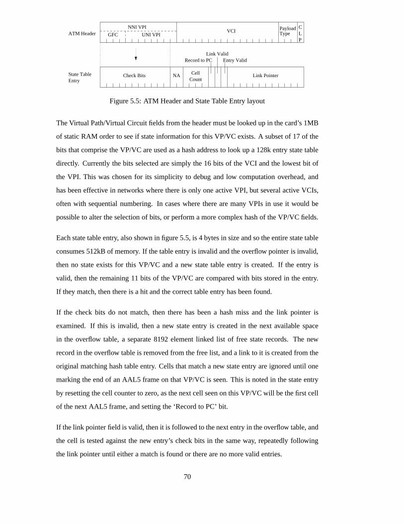
TypePayloadC

LP

ATM Header

CellCount

Link ValidEntry ValidRecord to PC

VCI

Link PointerCheck Bits NAEntryState Table

UNI VPIGFC

NNI VPI

Figure 5.5: ATM Header and State Table Entry layout

The Virtual Path/Virtual Circuit fields from the header mustbe looked up in the card’s 1MB

of static RAM order to see if state information for this VP/VCexists. A subset of 17 of the

bits that comprise the VP/VC are used as a hash address to lookup a 128k entry state table

directly. Currently the bits selected are simply the 16 bitsof the VCI and the lowest bit of

the VPI. This was chosen for its simplicity to debug and low computation overhead, and

has been effective in networks where there is only one activeVPI, but several active VCIs,

often with sequential numbering. In cases where there are many VPIs in use it would be

possible to alter the selection of bits, or perform a more complex hash of the VP/VC fields.

Each state table entry, also shown in figure 5.5, is 4 bytes in size and so the entire state table

consumes 512kB of memory. If the table entry is invalid and the overflow pointer is invalid,

then no state exists for this VP/VC and a new state table entryis created. If the entry is

valid, then the remaining 11 bits of the VP/VC are compared with bits stored in the entry.

If they match, then there is a hit and the correct table entry has been found.

If the check bits do not match, then there has been a hash miss and the link pointer is

examined. If this is invalid, then a new state entry is created in the next available space

in the overflow table, a separate 8192 element linked list of free state records. The new

record in the overflow table is removed from the free list, anda link to it is created from the

original matching hash table entry. Cells that match a new state entry are ignored until one

marking the end of an AAL5 frame on that VP/VC is seen. This is noted in the state entry

by resetting the cell counter to zero, as the next cell seen onthis VP/VC will be the first cell

of the next AAL5 frame, and setting the ‘Record to PC’ bit.

If the link pointer field is valid, then it is followed to the next entry in the overflow table, and

the cell is tested against the new entry’s check bits in the same way, repeatedly following

the link pointer until either a match is found or there are no more valid entries.

70

Once a cell is received that finds a valid hit in the state tables, the entry is examined to see

if this cell is one of the first N-th cells which are to be captured, and the Record to PC bit

is set. If so the FPGA is instructed to write the cell to the PC,and the cell counter in the

state entry for this VP/VC is incremented. If the cell is the last in an AAL5 frame, then the

counter is again reset to zero.

ATM UNI headers have a 8-bit VP and a 16-bit VC, or224 possible combinations, NNI

headers have a 12-bit VP for228 combinations. This particular scheme is limited to217direct hash entries and a further 8192 collisions, but more memory is available to increase

the size of the overflow table if necessary. In practice most ATM networks consist of only

a few hundred permanent virtual circuits (PVCs), since theyare hand configured, and are

seldom changed. The overflow table is more than large enough to handle this case, and

the hashing function of VP/VC bits can be carefully chosen toavoid collisions between

probable manual VP/VC allocations.

With a stable population of VP/VCs and few collisions, all ofthe valid state is likely to

reside within the StrongARMs 16kB data cache, allowing the code to run entirely at the

core frequency. When there are cache collisions, or new state entries are created, several

accesses to the external RAM are necessary, but there is timefor several RAM accesses

per cell arrival before the processing rate falls below the maximum cell arrival rate even at

OC-12c.

In the case where an ATM network utilises switched virtual circuits, a new VP/VC is poten-

tially allocated automatically for each TCP connection, and freed at the end of the session.

This leads to potentially large number of active VP/VCs simultaneously, and would require

a mechanism for detecting and garbage collecting the state tables periodically. If the num-

ber of active VP/VCs were to approach or exceed217 then there is insufficient memory

available on the Dag 3 to keep state information, and this task would have to fall to the host

PC with its larger resources.

5.5.3 Time Formatting and Synchronisation

Previous Dag cards used a simple free-running 32-bit counter to generate time-stamps, with

in-band synchronisation indication for drift correction and multi-card alignment in post-

71

processing. These counters ran at various rates, including4, 8, 16, and 12.5 MHz on dif-

ferent hardware at different times. Since the counters wereonly 32 bits long, they would

overflow and wrap back to zero in less than an hour, which was often during a measurement

run.

Relying on post-processing the time-stamps however reduces the amount of analysis that

can be done in real-time. Other difficulties are that time-stamps are are not absolute, instead

being relative to the beginning of the measurement. From thetime-stamps alone, it is not

possible to tell what frequency was used to increment the clock. This information must be

stored as well as the actual trace information.

For the Dag 3, a new time-stamping system was required to address these issues. The

Dag Universal Clock Kit (DUCK) was devised to address these issues, to produce cell or

packet time-stamps that are both precise and accurately synchronised to an external source

in real-time. I was involved in generating the requirementsfor the DUCK and specifying the

interface. The DUCK FPGA code was first implemented by Jed Martens, while I developed

the device driver support and the synchronisation feedbackloop, described later.

Time-stamp Format

The DUCK time-stamp is 64 bits long and little-endian. Making the time-stamps 64 bits

wide solves the overflow problem, and allows time-stamps within a measurement trace to

be manipulated more easily. For instance, time deltas can befound directly by subtracting

any two time-stamps. Little-endian format was chosen because the host processor for the

Dag cards is usually natively little-endian. Shown in figure5.6, the most significant 32 bits

of the time-stamp represent the number of seconds since midnight, January 1, 1970, the

same as a UNIXstruct time t. The least significant 32 bits form a binary fraction,

representing the fractional part of the time-stamp in the specified second.

Sign Bit

Seconds since Epoch (31 bits) Binary Fraction (32 bits)

Figure 5.6: Dag Time-stamp Format

72

The entire 64-bit time-stamp can be considered to be a fixed point number in seconds, or

it can be considered an integer count of time in units of2�32 seconds. Time deltas can be

computed directly by a single 64-bit subtraction. This can even be done between different

trace files if the clocks are synchronised, as time-stamps are now absolute, not relative to

the start of the measurement trace.

The time-stamp used by Dag is very similar to the one used by NTP, the only difference

between them is the different epoch used; NTP starts from Jan1st 1900, Dag with Jan 1st

1970. This gives the Dag time-stamp a lifetime as along long int type until Jan 19th

2038, when time overflows from the most significant bit of the 63-bit signed integer into the

sign bit which would represent a date before 1970. It is possible to interpret the 64-bit time-

stamp as a 64-bit unsigned integer instead, but extra care must be taken to avoid arithmetic

errors when comparing two time-stamps by subtraction.

The 32-bit binary fraction allows effective time-stampingclocks as high as232Hz (approx-

imately 4GHz), or a precision of approximately 250ps, allowing future compatibility with

high speed hardware, while allowing current clocks to run atintermediate speeds without a

change in time-stamp format.

Clock Generation

Dag cards do not yet have a 4GHz clock oscillator on them, and so cannot reach the full

resolution of the binary fraction. The Dag 3.2 series of cards instead have a 64MHz oscil-

lator, which is divided by two within the FPGA to produce a 32MHz clock signal for the

DUCK. This is referred to as theCrystal Frequency(f ). This clock signal is fed into a pro-

grammable divider that can produce a range of frequencies from 0–32MHz. The Dag 3.2

by default produces a time-stamp clock that runs at224 (16,777,216) Hz to provide 24 valid

bits of time-stamp fraction. This means that the 64-bit time-stamp increments by 0x100, or

approximately 60ns every tick. This clock is referred to as theSynthetic Frequency(fs), as

it is generated from the crystal oscillator on the board.

The crystal oscillator that is used is only accurate to�100 parts per million, or�100 mi-

croseconds per second. This error could compound to�0:36 seconds in one hour. This is

especially a problem when two cards are being used to capturetraffic from both directions

73

of a bi-directional link, as the Crystal Frequencies on the two cards will be different. With-

out clock correction, the time-stamps from the two traces will not match up, and cells or

packets will not fall in the same sequence that they appearedin on the fibre.

The Synthetic Frequency can be finely adjusted to take account of the inaccuracy of the

crystal oscillator, allowing the clock to be corrected and synchronised if a master clock or

frequency reference is available.

Clock Inc refers to the amount that the binary fraction will incrementfor each tick of the

Synthetic clock. In the case where the Synthetic Frequency is 16,777,216 Hz, this will be

0x100. Clock Wraprefers to the value of the binary fraction at which time the 32most

significant bits increment. This is currently always 0xffffffff, but in the future may be pro-

grammable to allow the use of different time-stamp formats.

TheDDS Rate(DDS) is a 32-bit number used to generate the Synthetic Frequencyfrom

the Crystal Frequency in equation 5.1. DDS refers to Direct Digital Synthesis, the method

used to generate the Synthetic Frequency.fs = f �DDS232 (5.1)

Figure 5.7 illustrates the mechanism that the DUCK utilisesto produce its Synthetic Fre-

quency from the available Crystal Frequency. On each edge ofthe Crystal Frequency signal,

a 32-bit adder adds the DDS Rate number to the value in the accumulator. The overflow

output from the adder is used to toggle the chip enable input on the time-stamp counter,

allowing it to be incremented. This is effectively the Synthetic Frequency output signal.

If the desired output frequency was exactly half the input frequency for instance, the DDS

Rate would be set to 0x80000000. On the first edge, the accumulated value rises from 0

to 0x80000000 and the counter is not enabled. On the next edge, the accumulated value

overflows to zero and the counter is enabled, hence causing the counter to count at half the

input frequency, thereby dividing the input signal by two.

For DUCK operation on the Dag 3 series, the desired SyntheticFrequency is224, slightly

over half of the Crystal Frequency, so the DDS Rate is calculated as above to be slightly

more than 0x80000000. The procedure operated as before, except that after the first count,

74

CrystalFrequency

32−bit

32−bit

+

Accumulator

DDS_Rate

CE

Overflow

ZerosTime−stamp Counter

56−bit64−bit

Sum

Figure 5.7: Dag 3 DUCK Clock Generator

the value in the accumulator is not zero but twice the difference between the DDS Rate and

0x80000000. This accumulated value represents the error between the actual output and the

desired output as a fraction over232.The accumulated error value has no effect until it passes a value of 232� DDS Rate, an

error equivalent to the period of the Synthetic Frequency. At this point an extra pulse in

the output is generated, reducing the accumulated error to near zero. This process can be

observed in figure 5.8, a simulation of the DUCK operation. Itcan be seen that the error

between the desired and actual output signals never accumulates to more than the period of

the Crystal Frequency, or 31.25ns for the Dag 3 DUCK, and has an average value half that.

This must be considered a random measurement error, but is small in magnitude. Since cell

arrivals are asynchronous to the measurement clock, a further random error is added in that

the time-stamp recorded for any arrival is the value of the time-stamp counter on the first

rising edge after the cell arrival.

Clock Synchronisation and Correction

The clock generation system described above can be used to generate an arbitrary desired

frequency from any fixed input frequency. It is also possiblehowever to adjust the DDS

Rate variable in order to maintain a stable output frequencywhere the input frequency

is unstable. This is very useful as the crystal oscillators used as sources for the Crystal

Frequency exhibit jitter and are temperature sensitive.

75

0 125 250 375 500 625 750 875 1000Time (nanoseconds)

Crystal

Overflow

Desired

Figure 5.8: Dag 3 Clock Waveform Comparison

FPGA configurations that include the DUCK form a control loopwith the Dag device driver

to synchronise the Synthetic Frequency to a reference clock. The control loop algorithm in

the Dag device driver adjusts the DDS Rate initially in a Frequency Locked Loop (FLL) and

then a Phase Locked Loop (PLL) to minimise the offset of the Dag time from the reference

clock.

The reference clock for the DUCK can be selected from 4 PPS sources. One of the sources

is a RS422 differential serial port. This port can be connected to the output of another Dag,

or to an external reference, such as a GPS receiver or CDMA cellular time receiver.

Another input source is the host PC, via software. This is mostly useful for debugging, but

could possibly be used in a NTP environment. The third input source is the time-stamp

counter itself. Using this input will generate a signal every time the most significant 32 bits

of the clock increment, or once per second. This can be used asa master signal for another

Dag card when no external PPS source is available, making it possible to synchronise the

two Dags to each other so that there is no relative error between the cards even if there is

some absolute error. The fourth input is an auxiliary input to the FPGA. It is intended that

in the future the 8kHz SONET frame signal will be routed to this input on cards that support

it, and divided in the FPGA by 8000 to produce an accurate 1Hz frequency reference.

76

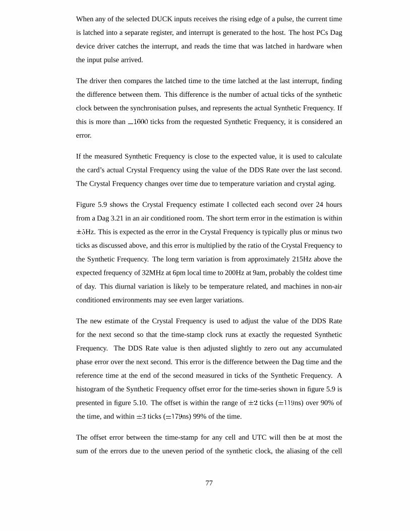
When any of the selected DUCK inputs receives the rising edgeof a pulse, the current time

is latched into a separate register, and interrupt is generated to the host. The host PCs Dag

device driver catches the interrupt, and reads the time thatwas latched in hardware when

the input pulse arrived.

The driver then compares the latched time to the time latchedat the last interrupt, finding

the difference between them. This difference is the number of actual ticks of the synthetic

clock between the synchronisation pulses, and represents the actual Synthetic Frequency. If

this is more than�1000 ticks from the requested Synthetic Frequency, it is considered an

error.

If the measured Synthetic Frequency is close to the expectedvalue, it is used to calculate

the card’s actual Crystal Frequency using the value of the DDS Rate over the last second.

The Crystal Frequency changes over time due to temperature variation and crystal aging.

Figure 5.9 shows the Crystal Frequency estimate I collectedeach second over 24 hours

from a Dag 3.21 in an air conditioned room. The short term error in the estimation is within�5Hz. This is expected as the error in the Crystal Frequency is typically plus or minus two

ticks as discussed above, and this error is multiplied by theratio of the Crystal Frequency to

the Synthetic Frequency. The long term variation is from approximately 215Hz above the

expected frequency of 32MHz at 6pm local time to 200Hz at 9am,probably the coldest time

of day. This diurnal variation is likely to be temperature related, and machines in non-air

conditioned environments may see even larger variations.

The new estimate of the Crystal Frequency is used to adjust the value of the DDS Rate

for the next second so that the time-stamp clock runs at exactly the requested Synthetic

Frequency. The DDS Rate value is then adjusted slightly to zero out any accumulated

phase error over the next second. This error is the difference between the Dag time and the

reference time at the end of the second measured in ticks of the Synthetic Frequency. A

histogram of the Synthetic Frequency offset error for the time-series shown in figure 5.9 is

presented in figure 5.10. The offset is within the range of�2 ticks (�119ns) over 90% of

the time, and within�3 ticks (�179ns) 99% of the time.

The offset error between the time-stamp for any cell and UTC will then be at most the

sum of the errors due to the uneven period of the synthetic clock, the aliasing of the cell

77

18:00:00 00:00:00 06:00:00 12:00:00 18:00:00Time (HH:MM:SS NZST)

32000190

32000195

32000200

32000205

32000210

32000215

32000220

Est

imat

ed C

ryst

al F

requ

ency

(H

z)

Figure 5.9: 24 Hour Crystal Oscillator Drift

-5 -4 -3 -2 -1 0 1 2 3 4 5Offset error at end of second (ticks)

0

10000

20000

30000

40000

50000

Figure 5.10: 24 Hour DUCK Offset Error Distribution

78

arrival against the synthetic clock, and the offset error between the synthetic clock and UTC.

This error is measured and recorded at the beginning and end of each second, as shown in

figure 5.9. This total offset error can be further examined experimentally by comparing

time-stamps applied to a single traffic stream by two separate Dag cards, with both cards

connected to the same reference clock. A diagram of the experimental configuration is

provided in figure 5.11.

GPS Antenna

RX

PC

Dag Card

TX RXOptical Splitter

Dag Card

PC PC

Dag Card

Figure 5.11: Time-stamp Difference Experiment

The difference between the time-stamps for the arrival of the same ATM cell from both

Dag cards is the sum of the offset errors of both cards at that time. Figure 5.12 shows

the distribution of time-stamp differences for cells transmitted at full rate on OC-3c ATM

link. Because only data from one second is presented, the DDSRate is not varying during

this time. Since the DDS Rate is fixed, the Synthetic Frequencies of the DUCKs in the

two Dag cards are fixed for the measurement period. The remaining differences are due

only to aliasing against the clock and the clock synthesis error. The Synthetic Frequencies

of the two DUCKs are not identical, and at the beginning of thesecond there is a small

offset between the DUCK clocks, which by the end of the secondthis has been reduced

to approximately zero. This reducing average offset over the second tends to broaden the

histogram.

By lowering the cell rate and sending a similar number of cells over 24 hours rather than

a single second, we can see the impact of the DUCK clock synchronisation mechanism

on the time-stamp differences, in figure 5.13. Note the log y-axis; all of the time-stamp

differences are within�2 clock ticks. The worst time-stamp difference was 9 Synthetic

Clock ticks, or approximately 540�s. During the measurement period the DUCK offset

error to the reference signal was examined at the end of each second, and the values of the

79

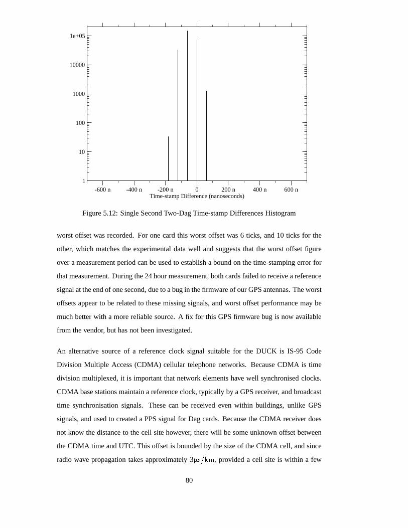
-600 n -400 n -200 n 0 200 n 400 n 600 nTime-stamp Difference (nanoseconds)

1

10

100

1000

10000

1e+05

Figure 5.12: Single Second Two-Dag Time-stamp DifferencesHistogram

worst offset was recorded. For one card this worst offset was6 ticks, and 10 ticks for the

other, which matches the experimental data well and suggests that the worst offset figure

over a measurement period can be used to establish a bound on the time-stamping error for

that measurement. During the 24 hour measurement, both cards failed to receive a reference

signal at the end of one second, due to a bug in the firmware of our GPS antennas. The worst

offsets appear to be related to these missing signals, and worst offset performance may be

much better with a more reliable source. A fix for this GPS firmware bug is now available

from the vendor, but has not been investigated.

An alternative source of a reference clock signal suitable for the DUCK is IS-95 Code

Division Multiple Access (CDMA) cellular telephone networks. Because CDMA is time

division multiplexed, it is important that network elements have well synchronised clocks.

CDMA base stations maintain a reference clock, typically bya GPS receiver, and broadcast

time synchronisation signals. These can be received even within buildings, unlike GPS

signals, and used to created a PPS signal for Dag cards. Because the CDMA receiver does

not know the distance to the cell site however, there will be some unknown offset between

the CDMA time and UTC. This offset is bounded by the size of theCDMA cell, and since

radio wave propagation takes approximately 3�s=km, provided a cell site is within a few

80

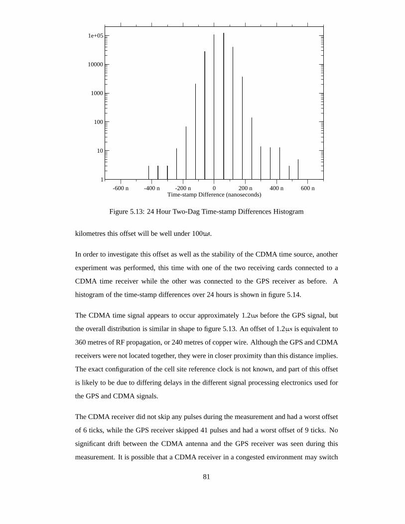
-600 n -400 n -200 n 0 200 n 400 n 600 nTime-stamp Difference (nanoseconds)

1

10

100

1000

10000

1e+05

Figure 5.13: 24 Hour Two-Dag Time-stamp Differences Histogram

kilometres this offset will be well under 100�s.In order to investigate this offset as well as the stability of the CDMA time source, another

experiment was performed, this time with one of the two receiving cards connected to a

CDMA time receiver while the other was connected to the GPS receiver as before. A

histogram of the time-stamp differences over 24 hours is shown in figure 5.14.

The CDMA time signal appears to occur approximately 1.2�s before the GPS signal, but

the overall distribution is similar in shape to figure 5.13. An offset of 1.2�s is equivalent to

360 metres of RF propagation, or 240 metres of copper wire. Although the GPS and CDMA

receivers were not located together, they were in closer proximity than this distance implies.

The exact configuration of the cell site reference clock is not known, and part of this offset

is likely to be due to differing delays in the different signal processing electronics used for

the GPS and CDMA signals.

The CDMA receiver did not skip any pulses during the measurement and had a worst offset

of 6 ticks, while the GPS receiver skipped 41 pulses and had a worst offset of 9 ticks. No

significant drift between the CDMA antenna and the GPS receiver was seen during this

measurement. It is possible that a CDMA receiver in a congested environment may switch

81

600.0 n 800.0 n 1.0 µ 1.2 µ 1.4 µ 1.6 µ 1.8 µTime-stamp Difference (nanoseconds)

1

10

100

1000

10000

1e+05

Figure 5.14: 24 Hour Two-Dag Time-stamp Differences Histogram, GPS vs CDMA

between available cell sites, causing jumps in the offset error, so it would seem prudent

to survey a proposed measurement site with both GPS and CDMA before committing to a

CDMA installation. By recording a time-series of the offsetbetween the CDMA and GPS

time standards, it should be possible to detect stepwise changes in offset indicating that the

CDMA receiver has switched cell sites. Knowing mean value ofthe difference between

GPS and CDMA time may also be important when performing high accuracy packet delay

measurements to or from a site.

5.5.4 Packet over SONET

ATM is by no means the only protocol used in high speed or wide area networking to carry

IP. Packet over SONET (POS) is a popular alternative for backbone links, including the

Abilene research network.

POS is an alternative method of carrying data packets over SONET, utilising the octet

synchronous HDLC protocol for encoding and framing. A 4-byte encapsulation header

is prepended to the payload data, and a 16 or 32-bit CRC is appended. Data packets are

stuffed according to HDLC byte-stuffing rules, in which the special flag character 0x7E

82

when occurring within a frame must be escaped by theescapecharacter 0x7D and then has

its sixth data bit cleared. The escape character when occurring in the frame data must also

be escaped in the same manner. The packet is then transmitteddirectly as SONET payload,

after optional scrambling.

The motivation behind the uptake of POS over ATM comes from several quarters. As POS

equipment is simpler than ATM, it may be less expensive. POS can also be implemented

directly on a SONET line where ATM service is not available. Perhaps most importantly,

POS can be more a more efficient link layer than Classical IP over ATM.

In Classical IP over ATM, IP packets are carried within AAL5 frames, and since an AAL5

frame must occupy an integer number of ATM cells, padding bytes must be added to fill

any excess space in the AAL5 frame. This inefficiency is dependent on the distribution

of packet lengths, and is especially aggravated by TCP acknowledgement packets. These

packets have an IP total length of 40 bytes, and packets of this length typically comprise

25–50% of IP network traffic. Figure 5.15 shows a distribution of IP packet lengths taken

from a 24 hour measurement of the University of Auckland’s Internet connection on the

21st of February 2001. The measurement used a pair of Dag 3.21s to capture 65,019,471

IP packets from the connection, which is provisioned over anATM circuit. It is clear that

40-byte packets are common, and comprise 33% of all packets recorded.

A 40-byte IP packet will have an 8-byte LLC/SNAP header prepended, taking up exactly

one cell’s payload space. Unfortunately, the 8-byte AAL5 trailer must still be appended,

requiring a second cell, the remainder of which is padded with zeros. In order to transport a

40-byte IP packet then, Classical IP over ATM transmits two cells or 106 bytes, an efficiency

of only 38%. Figure 5.16 shows a distribution of the number ofATM cells required to

transport the IP packets from the Auckland measurement. It can be seen that the peak of

40-byte IP packets has caused a peak in the number of two cell AAL5 frames.

Since short packets comprise only a small fraction of the total bytes carried on a network

link, the relatively higher efficiency of larger packets largely makes up for this, the re-

maining 10–20% efficiency loss is often referred to as theATM cell tax. In the case of

the University of Auckland measurement, of the total SONET payload used the IP packets

themselves comprised only 81%, 10% was due to AAL5 trailers and padding, and the final

9% was ATM cell headers, for a total cell tax of 19%.

83

0 250 500 750 1000 1250 1500IP Packet Length (Bytes)

0.0

5.0×106

1.0×107

1.5×107

2.0×107

2.5×107

Figure 5.15: IP Packet Length Distribution

0 5 10 15 20 25 30 35ATM packet Length (Cells)

0

1e+07

2e+07

3e+07

4e+07

Figure 5.16: ATM Packet Length Distribution

84

With the rising popularity of POS, the ability to measure POSlinks as well as ATM links

with the Dag 3 would then be a useful feature, however the PMC Sierra PM5355 physical

layer device used on the 3.2 series Dag is specifically designed as an ATM physical layer

and has no direct support for POS.

Jed Martens added support for POS to the 3.2 series Dags by using a raw mode of the

physical layer device. In this mode the PM5355 physical layer simply passes all SONET

payload bytes to the FPGA in 53-byte units. Once 53 bytes of SONET payload have been

received, a ‘cell arrival’ event is signalled to the FPGA, and the FPGA reads the next 53

bytes of SONET payload out as if it were an ATM cell.

In order to time-stamp and extract the IP headers from this data stream, the FPGA must

implement a POS physical layer receiver. The incoming SONETpayload is optionally

passed through a self-synchronising descrambler, and theninto an HDLC receiver state

machine which detects frames and performs byte unstuffing. The time-stamp for the POS

frame is generated from the frame detection logic, and the HDLC frame is built into a packet

record in much the same way as ATM cells are for delivery to thePC.

This scheme allows the 3.2 series Dag cards measure POS links, but unfortunately the limi-

tation of the physical layer in presenting the SONET data in 53-byte chunks causes a loss of

accuracy in the packet time-stamps, especially at OC-3c. When measuring cells on an ATM

link, the cell time-stamp is recorded on the signal from the physical layer device that a cell

has arrived and is available to be read. This guarantees a high accuracy time-stamp, and the

cell is then read out from the physical layer device at a higher bit-rate than a OC-12c link,

guaranteeing that there is never more than one cell queued inthe physical layer. This same

rate is used for both OC-3c and OC-12c links.

POS frames however are of arbitrary length, and are not aligned to the 53-byte chunks

that the physical layer device divides the POS byte-stream into, so the cell available signal

cannot be used to time-stamp the POS frames. Since POS framescan be shorter than 53

bytes, it is even possible to have the start of two different frames within one 53-byte chunk.

The POS frame is time-stamped after the start of frame has been detected in the FPGA after

the descrambling stage. The 53-byte chunks are read out on a 50MHz bus 16-bits wide, a

bandwidth of 100MB/s, over five times the bandwidth of OC-3c POS. This means that the

time-stamp of a POS frame beginning near the end of the 53-byte chunk may be incorrect

85

by up to 4/5 of a cell time at OC-3c, or approximately 2.2�s.Idle Idle

Read Out Read Out Read Out

Idle

Read Out

ATM Cell Time ATM Cell Time ATM Cell Time ATM Cell Time

POS Frame POS Frame POS Frame

a)

b)

c)

Figure 5.17: POS OC-3c Timing Error on Dag 3.21

Ignoring SONET line overheads, figure 5.17 is a timing diagram to scale of this effect for an

OC-3c POS link. The top time-line a) shows an OC-3c link with three POS frames present.

The first represents a 70-byte IP packet, the second a 28-byteIP packet, and the third a

40-byte IP packet. In POS networks the gaps between frames are filled with flag characters.

Time-line b) shows how the data on this line might be divided by the physical layer device

into arbitrarily aligned 53-byte chunks. The bottom time-line c) shows how after 53 bytes of

network data, including start characters has been collected, it is read out from the physical

layer at a much higher rate than the network.

The frames are each time-stamped when the first byte of the frame appears on this last time-

line, the red lines indicate the offset of this from the actual arrival time of the frame. It

is clear that the second and third frames both start within one chunk, and so will receive

time-stamps that are much closer together than they should be. This may cause significant

difficulty in packet inter-arrival time analysis.

For OC-12c POS links this effect is much reduced, due to the smaller disparity between

the network rate and the data rate of the physical layer bus. The largest time-stamp error

induced in this case will be approximately 1/5 of a cell time at OC-12c, or 152ns.5.5.5 Ethernet

Ethernet is generally considered a LAN technology, howeverit is seeing increasing use as

a medium to deliver IP services to clients from ISPs with MAN environments. Ethernet

is widely deployed within campus networks and LANs, making it easily accessible by re-

86

searchers. Often a site’s external network connection runsover a single Ethernet link at

some point, making it a desirable point for network measurement.

A prototype Dag to measure Ethernet links was built based on the Dag 2, but problems

with the ICS1891 physical layer chip-set at 10Mb/s speeds meant that few Dag 2.1E cards

were built. The Dag 3.2E, figure 5.18, used a newer physical layer device and has been

very successful. The 3.2E differs from all other Dag cards inthat it has two physical layer

interfaces instead of one, and is capable of performing measurements on both interfaces

simultaneously.

TX

RX

TX

RX

ICS1893EthernetASIC

ICS1893EthernetASIC


Xilinx

4062

FPGATiming signal

FIFO

512k

Switch

10/100baseTNetwork

10/100baseTNetwork

StrongARM

233MHz

512k EEPROM

1MB SRAM

System Bus

(32 bit 33MHz)

Figure 5.18: Dag 3.21E Block Diagram

The Dag 3.2 buffering, processing, and PCI connection back-end were designed to handle

over 600Mb/s from an OC-12c, so two interfaces at 100Mb/s each are easily within its

capabilities but would have over-stressed the Dag 2 design.The benefit of having two

physical layer devices on the card was to allow a single Dag card to measure both directions

of a full-duplex link simultaneously. As well as saving on post-processing to merge the

traces from two cards, this approach would use fewer PCI slots in the PC, and would be

more cost effective, an important requirement in academic environments.

The card physically has two network ports, and an analog switch that allows the transmit

path from each physical layer device to be sent either to the same port as the receive path

from that device, or to the other network port. In the first case each physical layer operates

as a normal independent Ethernet end-point station. In the second case, the physical layer

devices can be set tofacility loop-backmode. This causes the packets being received from

87

the network to be immediately retransmitted on the transmitpath to the other network port.

With both physical layers in this mode, the Dag card could be inserted into a full-duplex

Ethernet connection, with each of the original pair of devices connected to one of the Dag

ports.

This allows the Dag to measure packets travelling in both directions on the link, one direc-

tion from each physical layer. The disadvantage of this method however is that if the card

was turned off, the analog switch was incorrectly set, or thephysical layer devices were

not configured for facility loop-back, then the connection between the two communicating

Ethernet devices was broken. Although acceptable in a test-bench environment, this could

not be used on important links such as campus backbones due tothe risk of causing network

outages.

An alternative method for measuring full-duplex Ethernet connections is to use a passive

electrical tap. This maintains a permanent electrical connection between the Ethernet de-

vices so that there can be no service interruption due to power loss or misconfiguration of

the Dag. Figure 5.19 shows one direction of such a tap betweendevice one and device two.

This circuit is duplicated for the signal pair in the opposite direction. All resistors shown

are 16.6 ohms, both the Dag and the two device receive ports have an input impedance of

100 ohms.

Device 2 RXDevice 1 TX

Dag Port A RX

Figure 5.19: Resistive Ethernet Tap

Unfortunately because of the resistive network used to perform impedance matching, one

half of the signal power is lost as heat, and one quarter goes to the Dag port, leaving only

one quarter of the original signal power available for the destination Ethernet device. This

high insertion loss of 6dB could cause problems with long runs of cable, as the IEEE 802.3

10baseT Physical Coding Sublayer (PCS) standard specifies amaximum end-to-end inser-

tion loss of 11.5dB, and 0.5mm (24AWG) Ethernet cable typically exhibits an attenuation

at relevant frequencies of 8–10dB/100m at 20ÆC.

88

A future Ethernet Dag design will likely resolve this problem by placing the network tap in-

ternally on the Dag card, using a high impedance tap to accessthe Ethernet signals, leading

to much lower insertion loss as well as simplified cabling.

In cases where the Ethernet is not full-duplex, either because the devices do not support it,

or a hub is in use creating a collision domain, the two ports ofthe Dag 3.2E can be used

independently to measure two different network segments. This allows a single card to

measure delay through network equipment such as routers andfire-walls, provided Ethernet

interfaces are present.

5.5.6 The Dag 3.5

By 2001 the Dag 3.2 design was over two years old, and some parts used in their design

were becoming difficult to obtain and in the intervening timeimprovements in the capability

and cost efficiency of FPGAs had been made. The Dag 3.5 series,figure 5.20, is the next

generation of Dag 3 cards, intended primarily to operate thesame interfaces as the 3.2 series

with similar features, but with newer components and at lower cost.

TX

RX

Spartan−IIXilinx

FPGA


Network

OC−12c

OC−3c or

512k EEPROM

StrongARM

233MHz

System Bus

(32 bit 58MHz)

1MB SSRAM

Xilinx

Spartan−II

FPGA

Timing signal

1MB SSRAM

Multiplexer/

Demultiplexer


The two Xilinx Spartan-II devices used in the Dag 3.5 design each contain over double the

number of programmable gates as the FPGA used on the 3.2 Dags.The new FPGAs are

also physically smaller, are able to be clocked faster, and are less expensive than the older

parts. The gates are well spent on the 3.5 design, as another major difference is that the

89

ASIC physical layer device has been replaced with an FPGA. This FPGA must incorporate

SONET termination logic as well as descramblers and physical layer logic for either ATM

or POS SONET payloads.

This FPGA based physical layer solves the time-stamping problems encountered with POS

on the 3.2 design, as the DUCK time-stamping system is located within the same device as

the physical layer, allowing packet arrivals to be time-stamped directly. Since the SONET

handling is now programmable, the Dag 3.5 could be used on non-concatenated circuits,

that is to measure protocols carried on various different fractions of a multiplexed OC-3 or

OC-12 line. This reprogrammable nature also makes it possible to add support for other

transport protocols such as Cisco’s Dynamic Packet Transport (DPT) to be added after the

physical design of the hardware is complete.

The use of synchronous static RAM on the processor bus allowsthe bus to be run at the

higher rate of 58MHz, a 75% bandwidth improvement over the 3.2 Dags. This will allow the

StrongARM processor to perform more bus operations either to memory or to the FPGAs

during each packet arrival time, increasing the amount of useful work that can be performed

on the card. The hardware FIFO of the Dag 3.2 has been replacedwith faster synchronous

static RAM, with twice the capacity. The use of RAM requires the FPGA to generate

addressing signals that are unnecessary with FIFO memory, but the added flexibility is

worthwhile. By using RAM in place of a FIFO device, the contents of the buffer can be

accessed and updated randomly rather than in a strictly sequential manner. This allows the

modification of packet header records with information discovered after the record has been

written to the buffer, such as the packet length or CRC validity.

Variable Length Records

Previous Dag cards always produced a fixed size record for each packet arrival, typically

64 bytes, containing the time-stamp, packet length, and a fixed number of bytes of packet

content. This makes the resulting trace file of fixed length records simple to index, search,

subset or merge as the offset of the Nth packet record within atrace can be calculated

directly.

Fixed length records are not always the best solution for particular measurement applica-

90

tions however. A fixed length may be too short to record headers with options appended,

or application level protocols such as HTTP Get requests. Likewise, in some applications

security considerations dictate that no payload data should be captured at all. In this case

fixed length records may include some payload bytes that mustbe later blanked out in post-

measurement sanitisation procedures, and simply waste bandwidth and storage during the

measurement process.

Variable length packet records allow more flexibility in howmuch or how little should be

recorded from each packet on an individual basis. A variablelength record format however

makes searching trace files more difficult, and in order to navigate them at all the length of

the record should be placed in the record header. The RAM buffer of the Dag 3.5 allows this

to happen efficiently. As a packet arrives it is time-stamped, and the time-stamp is written

into the buffer as if it were a FIFO, followed by a blank space for the record length and the

start of the packet. When enough of the packet has been received to decode the protocols

and calculate the desired record length, further packet bytes can be discarded, and the FPGA

can insert the record length into the blank space at the startof the record. Hardware FIFOs

cannot be rewound in this manner to update the record header.Furthermore it is possible

once the entire packet has been received to add to the record header the length of the packet

on the network, and even to optionally discard the entire record if the packet fails a CRC

test by setting the buffer write pointer back to the start of the record.

5.5.7 Applications

The Dag 3 series of network measurement cards has been the most successful Dag design

to date, with well over 100 produced for use by the WAND Group,research partners, and

private industry. This wide acceptance has been critical infunding further research and

development, and demonstrates the need within the researchcommunity for measurement

focused systems.

As well as research partners using Dag cards, the WAND Group has made a data-set

known as Auckland-IV available as part of the WITS. This data-set contains 47 individ-

ual traces comprising almost complete coverage of a 49 day period starting 20th February

2001 [Micheel et al., 2001]. With a total over over 3 billion IP headers recorded, this archive

is expected to be a very useful research tool in the future.

91

5.6 The Dag 4

In late 1998, the Cooperatve Association for Internet Data Analysis (CAIDA) approached

the Dag group to develop OC-48c network measurement technology. This initiative led to

the Dag 4 series of cards. Design work began in May 1999, on thefirst Dag 4 prototype, the

Dag 4.0. This was intended primarily to be a test-bed for the design of the network interface

part of the card. For this reason it used the same processing and PCI back-end as the Dag

3.2, the changes being in the optics and physical layer device. An extra FPGA was added

before a FIFO memory in order to perform time-stamping, offloading the PCI FPGA. In

August the design was sent to be fabricated, however long delays ensued due to difficulties

with purchasing some of the components. In February 2000 theDag 4.0 returned from the

manufacturer, and testing could begin.

Although successful as a learning exercise, the Dag 4.0 was capable of ATM reception only,

and was limited to less than full line rate due to its 32-bit 33MHz PCI interface. With the

experience gained from the 4.0, the Dag 4.1 was designed, andsent for manufacture in July

2000. Shown in figure 5.21, the Dag 4.1 employed an updated physical layer device that

would allow POS measurement, more FPGAs with greater capacity each, a 64-bit 66MHz

PCI interface capable of meeting bandwidth demands, and a faster ARM processor bus.

TX

RX

512k EEPROM

PreprocessorFPGA

Single Mode OC48cTime Signal

PCI Bus (64 bit 66 MHz)

FIFO ATM/PoSFramer

MultiplexerPCI/DMAFPGA

Data ProcessingFPGA

1MB SSRAM

1MB SSRAM(32 bit 50 MHz)

System Bus

StrongARM

233MHz

(8 bit 10 MHz)

Peripheral Bus


The first Dag 4.1 was available for development in November 2000. With three large FPGA

devices, the Dag 4.1 is considerably more complex than any previous Dag card, and with

92

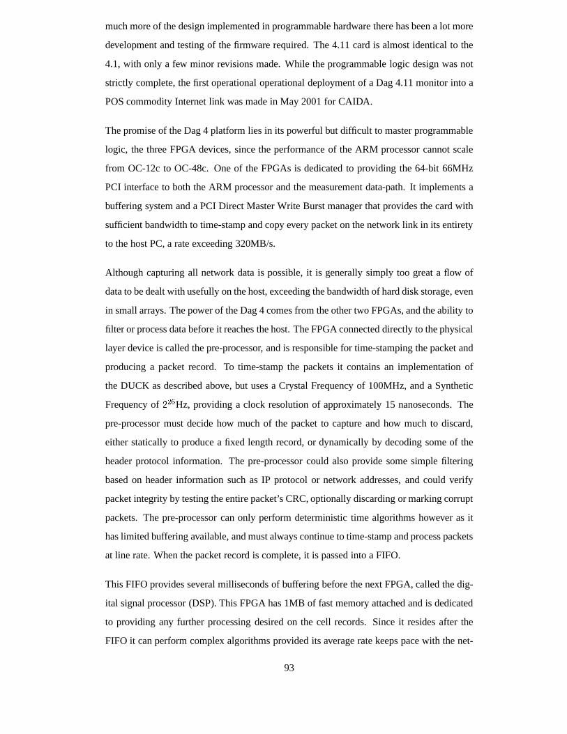
much more of the design implemented in programmable hardware there has been a lot more

development and testing of the firmware required. The 4.11 card is almost identical to the

4.1, with only a few minor revisions made. While the programmable logic design was not

strictly complete, the first operational operational deployment of a Dag 4.11 monitor into a

POS commodity Internet link was made in May 2001 for CAIDA.

The promise of the Dag 4 platform lies in its powerful but difficult to master programmable

logic, the three FPGA devices, since the performance of the ARM processor cannot scale

from OC-12c to OC-48c. One of the FPGAs is dedicated to providing the 64-bit 66MHz

PCI interface to both the ARM processor and the measurement data-path. It implements a

buffering system and a PCI Direct Master Write Burst managerthat provides the card with

sufficient bandwidth to time-stamp and copy every packet on the network link in its entirety

to the host PC, a rate exceeding 320MB/s.

Although capturing all network data is possible, it is generally simply too great a flow of

data to be dealt with usefully on the host, exceeding the bandwidth of hard disk storage, even

in small arrays. The power of the Dag 4 comes from the other twoFPGAs, and the ability to

filter or process data before it reaches the host. The FPGA connected directly to the physical

layer device is called the pre-processor, and is responsible for time-stamping the packet and

producing a packet record. To time-stamp the packets it contains an implementation of

the DUCK as described above, but uses a Crystal Frequency of 100MHz, and a Synthetic

Frequency of226Hz, providing a clock resolution of approximately 15 nanoseconds. The

pre-processor must decide how much of the packet to capture and how much to discard,

either statically to produce a fixed length record, or dynamically by decoding some of the

header protocol information. The pre-processor could alsoprovide some simple filtering

based on header information such as IP protocol or network addresses, and could verify

packet integrity by testing the entire packet’s CRC, optionally discarding or marking corrupt

packets. The pre-processor can only perform deterministictime algorithms however as it

has limited buffering available, and must always continue to time-stamp and process packets

at line rate. When the packet record is complete, it is passedinto a FIFO.

This FIFO provides several milliseconds of buffering before the next FPGA, called the dig-

ital signal processor (DSP). This FPGA has 1MB of fast memoryattached and is dedicated

to providing any further processing desired on the cell records. Since it resides after the

FIFO it can perform complex algorithms provided its averagerate keeps pace with the net-

93

work. The DSP’s output is sent to the PCI FPGA to be sent to the host. At the moment the

DSP is configured to simply pass the cell records arriving from the pre-processor on to the

PCI FPGA unchanged, but in the future it could be configured toperform more complex

filtering or classification of packet records, or to collect statistics on the fly.

To perform complex filtering the DSP might implement a processor designed to natively

execute a packet filtering language such as BPF+. Another approach would be to translate

the desired packet filter program into VHSIC Hardware Description Language (VHDL)

code, and then compile an image for the DSP FPGA that implements the filter directly.

Simple statistics keeping might involve counting bytes fordifferent protocols, or building

histograms. More sophisticated processing might involve building and maintaining flow

tables, and generating flow statistics, or performing longest prefix matching to translate

IP addresses to AS numbers in order to build AS-AS matrices. Determining the exact

capabilities of the Dag 4 will require further research and development.

5.7 Dag Software and Device Driver

The early measurement work done with the ATML ISA and PCI NICs(x5.1, 5.2) was done

in MS-DOS, as this allowed complete control over the PC and NIC hardware, and min-

imised latencies. No device driver as such was needed, the software that ran on the PC was

written in C to directly access the NIC’s registers as memoryaccesses. Captured network

data was read from the PC’s high memory via an extended memoryAPI, and written to disk

via BIOS calls. A software debugging monitor on the NIC allowed the reading and writing

of both the embedded processor’s memory and the control registers of the other devices

on the card such as the physical layer. This was used to configure the card for measure-

ment, and to command the NIC to execute the custom measurement program. Access to the

monitor was via a serial port on the NIC, initially manually via a dumb terminal and later

automatically from the host PC.

The Dag 1 (x5.3) was initially controlled and used in the same way. When the group decided

to build a stand-alone measurement card, the Dag 2 (x5.4), it was clear a new monitor would

be needed as the design was different to that of the Dag 1 and the source code to the monitor

used on the ATML NICs was not available. I wrote a monitor in ARM assembly language

94

from scratch that could initialise the card and allow software to be downloaded to the card

one byte at a time over the PCI bus, as the Dag 2 would have neither a serial port nor direct

slave accesses to the card’s memory from the PC to allow software downloads. The monitor

also provided read and write access to the card’s address spaces including the RAM and the

registers of the other devices on the card. This monitor was developed and tested on the

Dag 1 before the Dag 2 had been completed.

The need for a more versatile host platform than MS-DOS was becoming clear during the

use of the Dag 1, particularly the need for remote access bothfor control and accessing the

results of a measurement, as well as an improved developmentenvironment. Commercial

Real-time Operating Systems were investigated but the costwas prohibitive. A device driver

was written for Linux by Stele Martin as an experiment to determine if a UNIX-like OS

would interfere too greatly and unpredictably with the measurement process. This was

quite successful, and I rewrote the Linux driver for the Dag 2when it became available,

interfacing with the new monitor.

The Linux device driver is responsible for finding and initialising any Dag cards in a system,

handling interrupts from the card, and acting as an interface to the cards for user space pro-

grams. Finding Dag cards is accomplished by examining the PCI device tables provided by

Linux for the PCI vendor and device codes used by the cards. The driver then initiates com-

munication with each Dag’s monitor, performing some simplediagnostic tests and reporting

any errors. The Dag cards write captured data records to a region of physical memory on

the host that the Linux kernel is configured not to use for normal virtual memory allocation

at boot time. The Dag driver then remaps this memory space into the kernel, allowing user

space programs to read the cell records by memory mapping thespace once again. This

memory remapping scheme allows user space programs to read the cell records from the

physical memory locations to which the Dag card has written them, avoiding costly and

memory to memory copies.

As well as memory mapping the reserved capture memory, the Dag device driver offers

many functions to user space programs via IO control calls. Functions exported in this way

include reading and writing both the RAM and peripheral address spaces on the Dag via

its monitor, which is used for debugging and downloading ARMsoftware and FPGA im-

ages, configuring the physical layer device, reading the state of the capture memory space,

resetting the Dag, and starting the execution of downloadedARM code.

95

During data capture, the Dag 2 interrupts the host every timea megabyte of records have

been written to the PC. The interrupt handler provided by thedriver then reads the location

of the buffer, and makes it available to user space programs via IO control calls or a select

interface. If the Dag 2 is connected to a reference clock source it will also interrupt the

host when a reference signal event occurs, allowing the driver to read from the card the

stored value of the time-stamping clock from the event. Thiscan be used in post processing

to correct the time-stamps in the capture session for the clock drift caused by the crystal

oscillator on each Dag.

The Dag 3 was the first to use a reprogrammable implementationof the PCI logic in an

FPGA rather than a separate ASIC. This allowed greater flexibility in the number of PCI

registers, and so I rewrote the device driver again to handleboth Dag 2 and Dag 3 cards with

different register maps more cleanly. The embedded monitorexecuted by the ARM proces-

sor on the Dag was also rewritten to deal with new features of the Dag 3 card including the

StrongARM processor and cache, and changed memory maps on the cards. The character

based command interface used by the earlier monitor and driver was replaced with a more

efficient and reliable binary protocol using several 32-bitregisters.

The driver developed for the Dag 3s was the first to implement the host side of the DUCK

(x5.5.3), including the clock control loop and monitoring in the interrupt handler, and IO

controls to allow user space configuration of the DUCK and thecollection of clock quality

statistics.

I developed a number of ancillary programs during the courseof Dag development, to per-

form such tasks as downloading ARM software and FPGA images to the Dag, configur-

ing the physical layer device and the DUCK and reading SONET error statistics. The

dagsnap program performed the actual network measurements, configuring and starting

the capture process, then reading cell records via the memory mapped space in 1MB chunks

and writing them to disk files for storage and later analysis.

96

Chapter 6

Passive Calibration of Active

Measurement Systems

This chapter describes an experiment designed to compare the One-way-Delay results gen-

erated by a software based active measurement system with One-way-Delay measurements

of the same packets by a passive hardware based system.

6.1 One-Way-Delay

Measuring the time taken for packets sent from one host to arrive at their destination host

requires the ability to detect these packets at both the source and destination, and to record

time-stamps from a common clock for each observation. The accuracy of any system de-

signed to perform this measurement will depend on its two necessary components; a com-

mon clock, distributed to the vicinity of source and destination host, and a mechanism to

observe the packets, and accurately attach a time-stamp to each observation from the dis-

tributed clock.

There are several mechanisms capable of providing a distributed clock. NTP is a software-

only approach, which calibrates a host’s clock to a server byexchanging packets over a

connecting network, and estimating the delay to and from theserver. A common server

could be used for both end-points, but more commonly separate servers would be used,

with each server depending on some external clock. This approach is however susceptible

97

to changing or asymmetric network delays, and so its accuracy is typically not expected to

be better than plus or minus 1ms offset from the time standard.

If higher accuracy is desired an alternative to a network based clock synchronisation method

must be used, such as providing a reference clock directly toeach end-point of the measure-

ment. This requires extra hardware, such as GPS or CDMA receiver, and may require the

mounting of an antenna on the exterior of the building. Although expensive and potentially

difficult logistically, such systems promise accuracies ofplus or minus 100ns or better to

UTC [Trimble, 1999].

Once a clock is available, a means of observing the packets and time-stamping them with

the clock is needed. If the kernel clock is being constrainedby NTP, then it can then be used

to time-stamp the packets directly as they are received by a conventional NIC. This may be

acceptable where a NIC is available for the desired network media, but extra uncertainty

in the time-stamps is added via the conditioning of the kernel clock, the NIC behaviour in

reporting packet arrivals, interrupt latency of the host, and variations in processing of the

packet arrival by the network stack.

A formal metric for One-way-Delay is defined by the IETF IPPM working group in RFC2679,

“A One-way Delay Metric for IPPM” [Almes et al., 1999]. This document defines a single-

ton metric calledType-P-One-way-Delaythat describes a single measurement of One-way-

Delay. Using this singleton metric, a sample metric is defined which refers to a sequence of

Type-P-One-way-Delay singleton delays measured at times taken from a Poisson process,

calledType-P-One-way-Delay-Poisson-Stream.

There are at least two implementations of active measurement systems to collect these met-

rics, by ANS [Kalidindi and Zekauskas, 1999], and by RIPE NCC[Uijterwaal and Kolk-

man, 1997]. By measuring the probe packets from these activesystems at their source and

destination with a passive measurement system such as a Dag,an independent observation

of One-way-Delay can be made. Such measurements can then be used to quantify the host

related error characteristics of the software based activemeasurement system.

98

6.2 Test Traffic Measurement System

Since 1997, Reseaux IP Europeens Network Coordination Centre (RIPE NCC) has been op-

erating a system called Test Traffic Measurements (TTM) for measuring One-way-Delay[Uijterwaal

and Kolkman, 1997]. TTM is an active measurement system which has implemented the

IPPM One-way Delay and One-way Loss metrics to perform independent measurements

of connectivity parameters in the Internet. After a successful development and pilot phase,

TTM became a regular RIPE NCC membership service in October 2000.

In TTM active probe packets containing time-stamps are sentfrom a dedicated measurement

PC running FreeBSD on the source network to a similar PC on thedestination network.

The TTM System is illustrated in Figure 6.1. Independent probe packets are sent from the

TTM system on the second network to the first to measure the One-way-Delay in the return

direction.

The probe packets are 128 bytes long, and contain a UDP frame with destination port 6000,

and a UDP payload of 100 bytes. This is the TTM systems Type-P definition for the Type-

P-One-way-Delay metric framework.

Network B

Testbox BTestbox A

GPS Antenna GPS Antenna

Border Router Border Router

Network A Internet

Figure 6.1: RIPE NCC Test Traffic Measurement System

Each TTM PC is equipped with a GPS receiver. This receiver outputs a short pulse every

second on the DCD control line of the PCs serial port. These pulses generate interrupts,

which are used by NTP to phase-lock the kernel system clock.

A user space daemon on the TTM PC schedules test probes. When aprobe is to be sent, the

packet is built in user space, and the kernel system clock is read. The time is inserted into

the packet, and it is passed into kernel space to be queued fortransmission.

99

After the probe packet is received by the destination TTM machine, it is time-stamped again

with the kernel clock, which is synchronised by the same GPS mechanism. The difference

between the time recorded in the packet, and the time of the packet arrival are subtracted to

produce a One-way-Delay measurement.

Data collected at the TTM machines is later retrieved from them to a central point. By

comparing the records from the source for packets sent, and from the destination for packets

received, One-way-Loss can also be determined.

The user space process on the source machine schedules probepacket transmissions. These

are sent at a low rate in order to avoid artificially loading the network, especially where the

number of TTM machines is large.

6.2.1 Calibration Methodology

The following sections use data from an experiment conducted from 00:00 UTC on the 12th

of October 2000 to 00:00 UTC on the 13th. Each TTM machine is a PC running FreeBSD.

The specification of each individual machine is different, both in the hardware, and the

version of the FreeBSD used. The details of the TTM machines used in this experiment

are detailed in Table 6.1. The GPS reference clock design is currently uniform across the

deployed machines.

Host Site OS CPUtt01 Amsterdam, Holland FreeBSD 2.2.8 Pentium 200MHztt47 Hamilton, New Zealand FreeBSD 2.2.1 Pentium II 233MHz

Table 6.1: TTM hosts used in calibration experiment.

In order to obtain an independent measure of the One-way-Delay between tt01 and tt47,

hardware based passive measurement systems were introduced onto the Ethernet segments

used by the measurement interfaces of each of the machines. This was done by attaching

the passive measurement system to the same Ethernet hub thatthe TTM machine already

used.

In each case the additional system comprised a PC containingDag 3.1E passive Ethernet

measurement card, and a separate GPS receiver. The GPS receiver connects directly to the

network measurement card to control its local time-stamping clock. One interface from the

100

Dag card is connected to a hub, along with the main Ethernet connection for the measure-

ment machine, and the TTM host.

The Dag 3.1E at the time of the experiment was limited by firmware in the amount of data

it could capture from each packet. The Dag 3.1E produces a 64-byte fixed length for each

Ethernet frame that is received, regardless of the frame’s actual length [Tree, 2000]. When

the per-record overhead (8-byte time-stamp plus 2-byte wire length) is subtracted from the

64-byte record, 54 bytes remain. This contains the first 54 bytes of the Ethernet frame,

once the preamble has been discarded. The DIX Ethernet II frame format, used at both

endpoints, defines a 14-byte header [DEC et al., 1982], including source and destination

MAC addresses, and a type field. The Ethernet payload fills theremaining 40 bytes of the

record. An IPv4 header with no options requires 20 bytes. TheTest Traffic probe packets

are carried by the UDP protocol, which has a 8-byte header. This leaves only 12 bytes of

UDP payload in the Dag record.

The Test Traffic probe packets observed have an IP total length of 128 bytes, or a UDP

payload of 100 bytes. This means that not all of the probe packet payload is contained within

the record returned by the Dag card. The Test Traffic probe packet format specifies that the

sequence and time-stamp information carried within the packet be placed at a random byte

offset within the UDP payload, and that an offset field shouldbe at the start of the UDP

payload in order to locate it.

This is done to try to make the packets less compressible, as this may affect the delay

results for network paths where one or more links are compressed at the hardware layer for

transportation. The consequence is that the TTM sequence number and time-stamp are not

captured by the limited length Dag record.

In order to record these important fields, it is necessary to simultaneously capture the TTM

probes with a system that can record the entire packet, even if its timing is less accurate.

Since the main Ethernet card for the Dag host is connected to the measurement hub along

with the Dag, it is sufficient to runtcpdumpwith a suitablesnap lengthset so as to ensure

the entire payload is recorded.

Over the experiment’s 24-hour period, the Dag cards captured all Ethernet frames to host

memory, and software on the host filtered these for packets ofType-P. Thetcpdump run

101

simultaneously on each Dag host used identical filter rules.

6.2.2 Transmission Latency

In the 24-hour experiment, tt01 transmitted a total of 58,498 probes to the various destina-

tions, and tt47 transmitted 58,500 probes. As each probe packet is transmitted by the TTM

machine, it is time-stamped by the Dag system, and the packetcontents are collected by

tcpdump. The time-stamp placed into the probe packet by the TTM system to represent

the time that the probe was sent is extracted, and compared tothe time-stamp recorded by

the Dag hardware.

In post processing of the data recorded by the Dag card and bytcpdump, the packet trace

data from the Dag card and fromtcpdump are compared by IP source and destination

addresses, as well as Id field in order to find matches. The TTM probe packet fields are

then extracted from thetcpdump record, and the time-stamp from the corresponding Dag

record. The difference between these time-stamps is the difference between when the TTM

System recorded the packet as sent, and the time that the packet actually left the source

TTM host. This difference is referred to below as thetransmission latency.

In the specification of Type-P-One-way-Delay, the delay is defined as the time taken be-

tween the first bit of the probe packet leaving the interface of the source machine, thewire-

arrival-time, to when the last bit of the probe has arrived at the destination network interface,

thewire-exit-time. This means that any time difference between the recorded transmission

time-stamp and the wire-arrival-time of the probe on the source network is considered an

error. The upper bound on this error is referred to asHsource. LikewiseHdestrefers to an

upper bound on the difference between the wire-exit-time ofthe packet at the destination

and the destination time-stamp.

The Dag 3.2E card records its time-stamp in hardware at the end of the first nibble of the

preamble, so the Dag time-stamp is the same as the IPPM definition of wire-arrival-time,

minus the length of the first preamble nibble. Figure 6.2 illustrates the time-stamp’s relation

to the packet transmission process.

The length of the Ethernet preamble is variable, as it is permissible for Ethernet bridge or

hub devices to add or drop bits of the preamble from the start of packets. Each repeater

102

Packet queued

System time

insertedPacketcopy

Time−stamp NICprocessing

Packetready for

transmission

Wait forquiet

Preambleend

MAC headerstarts

IP packetstarts

SFD MAC header

read

to OSPacket scheduledfor transmission

Packet copiedto NIC

createdPacket

ActiveTime−stamp

Time

IP PacketPreamble

Preamblestarts

Time−stampDag 3.2E

wire−arrival−timeIPPM

Figure 6.2: Packet Transmission Time-line

the packet traverses on the destination Ethernet must transmit a minimum of 56-bit times

of preamble, or a maximum of the received number plus 6. The Dag card does not record

the length of the preamble, so it is not possible to calculatethe exact time at which the IP

packet ends due to the uncertainty in the number of bytes between the time-stamp and the

end of the IP frame. The simplifying assumption is made for the purposes of calculation

that the preamble is always 7 bytes, plus the one byte SFD.

The IPPM definition of wire-arrival-time does not define whether the first bit of the packet

refers to the first bit of the IP packet, the link layer frame, or the physical frame. For the

purposes of this thesis the wire-arrival-time is taken to bethe first detectable part of the

physical layer packet. This means that the serialisation time of the physical or link layer

headers is not included in the measured transmission latency.

Figure 6.3 shows a time-series of transmission latencies per packet on a log scale. Although

some peak latencies surpass 10ms, the bulk of the samples fall below 200�s. The spikes in

transmission latency are not errors, they are actual measured latencies. There are a number

of possible causes of these spikes, including cross traffic on the hub, and scheduling effects

on the TTM host.

A histogram of transmission latency from 0–250�s is provided in Figure 6.4 showing the

compact distribution of the bulk of the transmission latencies measured. The TTM host tt01

has a transmission latency centred about 153�s, while tt47 is centred about 83�s.The offset between the two distributions is easily explained by the difference in processing

power between the hosts. Differences in the CPU bridge and PCI bridge may also con-

tribute, since the hosts use different motherboards with different chip-sets.

103

00:00:00 06:00:00 12:00:00 18:00:00 00:00:00

Time (HH:MM:SS UTC)

0.0

500.0 µ

1.0 m

1.5 m

2.0 m

2.5 m

3.0 m

Tx

Late

ncy

(sec

onds

)

tt01.ripe.nettt47.ripe.net

Figure 6.3: TTM Transmission Latency Time-series

0 50 µ 100 µ 150 µ 200 µTx Latency (seconds)

1000

2000

3000

4000

5000


Figure 6.4: TTM Transmission Latency Distribution

104

The 25–50�s spread of the bulk of the distribution may be caused be several factors, includ-

ing variations in host interrupt latency, the time to process the packet, or NIC behaviour.

Some NIC cards for instance will buffer received packets before delivering them to the host

for up to 100�s, in order to reduce the interrupt load on the host in times of high network

activity.

The distribution of transmission latency appears to be approximately normal, figures 6.5

and 6.6 show QQ plots of the latency distributions for tt01 and tt47 respectively. The plot

for tt01 shows evidence of slightly heavier tails than for a normal distribution, and some

asymmetry. The tt47 QQ plot shows slight asymmetry and just slightly lighter tails than

normal distribution, apart from a series of exceptional values on the right. It is likely that

these are due to a separate underlying mechanism, and may be best modelled as a separate

distribution of exceptional events. If this experiment hadbeen carried out using a software

based measurement system, it might have been assumed that these outlying values were

due to measurement error. The Dag measurement system provides confidence that outly-

ing measurements are an accurate representation of the systems behaviour and not due to

measurement error.

−3 −2 −1 0 1 2 3

0.00

012

0.00

014

0.00

016

0.00

018

0.00

020

0.00

022

0.00

024

0.00

026

Normal Q−Q Plot

Theoretical Quantiles

Sam

ple

Qua

ntile

s

Figure 6.5: TT01 Transmission Latency QQ plot

A cumulative histogram of the transmit latency focusing on the extreme latency values is

105

−3 −2 −1 0 1 2 3

0.00

006

0.00

008

0.00

010

0.00

012

0.00

014

Normal Q−Q Plot

Theoretical Quantiles

Sam

ple

Qua

ntile

s

Figure 6.6: TT47 Transmission Latency QQ plot

presented in Figure 6.7. In this figure, the latencies of the two hosts have been normalised

to each other by subtracting from each the median latency. This is justified as the measured

latency is assumed to consist of some fixed offset plus some varying component, and we

wish to compare the varying components. Host tt01 has an upper latency spread below 1ms

in 99.98% of measurements, and below 250�s in 99.97%. Host tt47 has 99.96% of points

less than 1ms from the median latency. 99.95% of measured latencies fall below 250�sfor this host. The maximum transmission latencies recordedwere 6.30ms and 11.93ms for

hosts tt01 and tt47 respectively.

Since a maximum length Ethernet frame takes 1.23ms on a 10Mb/s Ethernet, spikes less

than or equal to this value may be caused by the Ethernet NIC waiting for an existing

packet on the hub to end before it can transmit. Transmissionlatencies greater than this

value must be at least partially due to some other mechanism.Possibilities include the

TTM host processor scheduling some other task in between thepacket being time-stamped

in user space and the packet being sent to the NIC for transmission, or unusually long

interrupt latencies due to slow peripheral devices such as hard disk controllers.

It may be possible to reduce the magnitude of latency peaks byrewriting the application so

106

1e-05 0.0001 0.001 0.01

Transmit Latency (seconds)

0.995

0.996

0.997

0.998

0.999

1

Cum

ulat

ive

Pro

babi

lity


Figure 6.7: TTM Transmission Latency Cumulative Distribution

that it runs partly in kernel space. A loadable kernel modulecould be called to insert the

time-stamp into the packet, and queue it for transmission. The advantage is that kernel space

code is not pre-emptable, so scheduling concerns and context switches are avoided. In order

to make the time-stamp to transmission operation atomic, itmay be necessary to mask or

disable interrupt processing during this operation. This approach cannot solve latency due

to inaccuracies in the clock however, or cross traffic on the Ethernet media.

6.2.3 Transmission scheduling

Each TTM host transmits probe packets to 26 other TTM hosts, and each individual mea-

surement is an example of the singleton Type-P-One-way-Delay metric. RFC2679 specifies

only one sample metric for a sequence of singleton measurements, Type-P-One-way-Delay-

Poisson-Stream. In this metric, the probe packets to a specific destination host should be

sent at times taken from a Poisson process. This is referred to as Poisson sampling.

There are several advantages to using a Poisson process for scheduling measurements [Pax-

son et al., 1998]. Poisson sampling of a system does not lead to synchronisation. That

is, each sample is not predictable, so probes injected into the network cannot induce peri-

107

odic behaviour. Periodic sampling can fail to measure periodic behaviour in the network,

where the periods of the behaviour and the sampling are similar, or one is a multiple of

the other. Poisson processes can also be proven to be asymptotically unbiased, even if the

measurement process affects the network.

In order to implement Poisson sampling, the delays between sending probes should be in-

dependent and random with a common exponential distribution with rate�, equation 6.1.G(t) = �e��t (6.1)

In 24 hours, the TTM host sends approximately 2,160 probe packets to each of the desti-

nation TTM machines, or one every 40 seconds on average. Figure 6.8 shows the inter-

transmission times for the first 500 probes sent from tt01 to tt47 and from tt47 to tt01.

There are clearly regular periods when the system does not perform any measurements,

represented as high inter-transmission times.

0 100 200 300 400 500

Probe number

0

60

120

180

240

300

Pro

be In

ter-

tran

smis

sion

tim

e (s

econ

ds) tt01 to tt47

tt47 to tt01

Figure 6.8: TTM Inter-probe Spacing Time-series

Figures 6.9 and 6.10 show the distribution of the observed probe spacing between 0 and

70 seconds for tt01 and tt47. Overlaid is an exponential distribution with rate 1/40. It

is clear that the TTM system is not performing Poisson sampling of One-way-Delay, but

108

0 10 20 30 40 50 60 70 80

Inter-transmission time (seconds)

0

50

100

150

200

250

tt01 to tt47Exponential (rate=1/40)

Figure 6.9: TT01 Inter-probe Spacing Distribution

0 10 20 30 40 50 60 70 80

Inter-transmission time (seconds)

0

50

100

150

200

250

tt47 to tt01Exponential (rate=1/40)

Figure 6.10: TT47 Inter-probe Spacing Distribution

109

rather sampling distributed in some approximately Normal way about a mean of 40 seconds.

This distribution has likely been chosen for TTM because exponential distributions can on

occasion generate very long times between probes, a problemnot well addressed in the

definition of Type-P-One-way-Delay-Poisson-Stream.

6.2.4 Reception Latency

In the experiment as each packet from a remote TTM host arrives at its destination network,

it is simultaneously received by three Ethernet devices. The Dag card time-stamps the

packet from its hardware clock as soon as the SFD character isdetected. The packet is also

received by the Ethernet NICs in both the TTM host, and the Dagmeasurement system. The

NIC cards buffer the packet and check its CRC, possibly wait for more packets to arrive,

then interrupt the host. When the host services the interrupt, it passes the received packet

descriptors to the network stack, which time-stamps each packet using the system clock.

Any user space programs that are listening are then passed pointers to the packets.

On the calibration hosttcpdump records the entire packet to disk, while on the TTM host

the packet is examined immediately. If it is a valid TTM packet, it is recorded to disk. In

post processing, further tests are carried out on each recorded probe, to ensure it is suitable

for analysis. If the embedded NTP quality values, NTP’s own estimate of it’s offset error

and dispersion show the source TTM host’s NTP daemon was locked to its reference clock,

then the difference between the packet’s received time-stamp and the source time-stamp

stored in the packet are compared to find the One-way-Delay ofthat TTM packet.

For each probe arriving at the destination network, the TTM packet’s Id field can be found

in thetcpdump record, and the source and destination IP addresses of that packet along

with its IP Packet Id can be used to find the same packet in the Dag record. This allows

us to attach the Dag time-stamp to each TTM probe Id. The data recorded by the TTM

system for each packet during the experiment was made available by RIPE NCC. These

files record for each measurement probe the time-stamp of thereceiving TTM host, along

with the calculated TTM One-way-Delay, the TTM Id, and otherinformation such as clock

stability. By matching the probe records using the TTM Id fields between these two data

sources, the arrival time-stamps for the probe packet as recorded by the Dag and TTM hosts

can be compared.

110

The Dag 3.2E cards used in this measurement time-stamp packets on the first nibble of

the preamble. The IPPM definition of wire-arrival-time is when the packet has been com-

pletely received. We call the difference between the IPPM arrival time definition and the

time-stamp from the active system thereception latencyof the receiving host. Figure 6.11

illustrates the time-stamp’s relation to the packet reception process.

Time

Time−stampDag 3.2E

Preamble

Preamblestarts

Preamble

SFD

end

MAC framestarts

MAC header

startsIP packet

IP Packet

IP packetends

MAC frameends

CRC processingNIC

Interrupthost PC

Packetcopy

Interruptlatency code

System timeread

Time−stampActive

servicedInterrupt

wire−exit−timeIPPM

Figure 6.11: Packet Reception Time-line

In order to calculate the IPPM arrival time from the Dag time-stamp, it is necessary to allow

for the length of the packet, and the speed of the network. TheTTM measurement probes

are UDP packets with 100-byte payloads. With UDP and IP headers, this becomes a 128-

byte total-length IP frame. The assumption from section 6.2.2 of an 8-byte preamble is

made, which along with the Ethernet header size of 14 bytes plus a 4-byte CRC brings the

total to 154 bytes. For a 10Mb/s Ethernet this results in a necessary correction to the Dag

time-stamp of 123.2�s, or 12.32�s for a 100Mb/s Ethernet.

A time-series of the reception latency is presented in figure6.12. Since some packets will

be lost in transmission, we expect to receive fewer packets on average than we send. Host

tt01 received 51,808 probes, and tt47 received 54,616.

As in the previous section, the time-series shows the bulk ofthe reception latencies tightly

constrained within a narrow band about 50�s wide, with occasional peaks to many times

the median value.

A histogram of the receive latencies for tt01 and tt47 under 250�s is presented in figure 6.13.

The histogram drop lines are removed to make the overlappingarea clearer. A similar time

scale is used for comparison with figure 6.4. Host tt01 has a median receive latency of 35�s,and tt47 has a median of 26�s. It is hard to understand why the slower computer with the

10Mb/s Ethernet NIC is producing lower reception latency figures, but this effect may be

111

due to differing deferred interrupt schemes on the different NICs.

The distribution of latencies for tt01 appears to be bimodal. This could be caused by two

common code paths of slightly differing lengths, or by frequent interrupt masking of a

period equal to the distance between the peaks, approximately 50�s.The cumulative histogram of the receive latency focusing onthe extreme values is presented

in Figure 6.14. In this figure, the latencies of the two hosts have been normalised to each

other by subtracting from each the median latency. This is justified if we take the mea-

sured latency to consist of some fixed offset plus some varying component, and we wish to

compare the varying component. Host tt01 has a latency below1ms in 99.97% of measure-

ments, and below 250�s in 99.89%. Host tt47 does better with only one point above 1ms,or 99.998% of points below 1ms. 99.94% of measured latencies fall below 250�s for this

host. The maximum latencies were 1.55ms and 1.57ms for hosts tt01 and tt47 respectively.

The maximum receive latencies are less than the maximum transmit latencies seen in sec-

tion 6.2.2, and this likely corresponds to the impact of the scheduler. While the transmit

latency includes the possibility that the scheduler will run some other process before trans-

mitting the packet, when a packet is received the interrupt is dealt with immediately, in-

terrupting whatever process is currently scheduled. The major components of the receive

latency then must be the interrupt latency of the host, and the time taken by the host to pro-

cess the interrupt. This may include copying the packet fromthe NIC to the host’s memory,

but in modern systems the NIC often performs this operation by DMA before interrupt-

ing the host to indicate packet arrival. Other processing time may include packet integrity

checks such as Ethernet CRC or IP header checksum calculation.

6.2.5 End to End Comparison

Since TTM probes can be identified at both the sending and receiving end networks, it is

possible to match up the transmit and receive latencies per packet, to find the total difference

between the One-way-Delay as measured by the TTM system, andthe wire-time One-way-

Delay as measured by the Dag hardware. Table 6.2 shows the number of packets observed

being exchanged between the pair of TTM hosts tt01 and tt47 during the 24-hour experi-

ment. Figure 6.15 shows the time-series of Type-P-One-Way-Delays for the experiment as

112

00:00:00 06:00:00 12:00:00 18:00:00 00:00:00

Time (HH:MM:SS UTC)

0.0

500.0 µ

1.0 m

1.5 m

2.0 m

Rx

Late

ncy

(sec

onds

)


Figure 6.12: TTM Reception Latency Time-series

0 50 µ 100 µ 150 µ 200 µ 250 µTx Latency (seconds)

0

1000

2000

3000

4000


Figure 6.13: TTM Reception Latency Distribution

113

recorded by the Dag cards. This a useful reference when considering the significance of the

measurement errors.

Figure 6.16 shows the time-series of the sums of the transmission and reception latencies

per packet for all the TTM probes that were successfully recorded at both sites. Figure 6.17

is a histogram from 0 to 400�s in 1�s bins of the time-series data. The median total latency

in the tt01 to tt47 measurement is 192�s, while in the tt47 to tt01 direction the median is

117�s. The distribution about these medians in both cases is of similar shape, and falls

almost entirely within plus or minus 50�s. There are some excursions to extreme values,

with total latency reaching a maximum of 1.3ms. This is to be expected from the previous

examination of the bulk properties of all of the probes transmitted and received by each

host, where we attribute these to host behaviour. The slightly bimodal nature of the tt47 to

tt01 latency is due to the receive behaviour of tt01, as seen in figure 6.13.

It is immediately noticeable that the distributions of total latency are not equivalent, despite

being captured by the same pair of hosts. This is due to the fact that while one host is

generally faster then the other, the relative speedup in thetransmission and reception pro-

cesses between the machines is not even. Since the improvement in reception latency is

greater than the speedup in transmission, the measurement in which the faster host (tt47) is

receiving, (ie. tt01 to tt47) has the lower total latency.

The total time added to the TTM One-way-Delay measurements by the host behaviour and

the variation in this added time is, as expected, independent of the magnitude of the One-

way-Delay. The total latency experienced is dependent on the particular hosts used, and

will be largely independent of network conditions, although cross traffic or collisions at the

TTM hosts Ethernet ports can cause additional latency up to at least one maximum length

Ethernet frame per host.

The extreme values are always positive, that is in the measured end to end delays there

appear to be no delays measured by the TTM system that are lessthen the wire-time One-

way-Delay measured by the Dag system. This indicates that the TTM measurement of the

minimum delay over a path is likely to be reliable, although it will only be accurate to within

the 50�s variation in TTM accuracy observed.

Extreme values are rare; there are only two probes for which the total latency is more than

114

1e-05 0.0001 0.001

Receive Latency (seconds)

0.995

0.996

0.997

0.998

0.999

1

Cum

ulat

ive

Pro

babi

lity


Figure 6.14: TTM Reception Latency Cumulative Distribution

From To Sent Received Packet Losstt01.ripe.net tt47.ripe.net 2160 2121 1.81%tt47.ripe.net tt01.ripe.net 2160 2154 0.28%

Table 6.2: TTM End to End Probe Experiment

00:00:00 06:00:00 12:00:00 18:00:00 00:00:00

Time (HH:MM:SS)

0

0.2

0.4

0.6

0.8

1

One

-way

-Del

ay (

seco

nds)

tt01 to tt47tt47 to tt01

Figure 6.15: TTM Type-P-One-way-Delay measured by Dag cards

115

00:00:00 06:00:00 12:00:00 18:00:00 00:00:00

Time (HH:MM:SS)

0.0

500.0 µ

1.0 m

1.5 m

Tot

al L

aten

cy (

seco

nds)

tt01 to tt47tt47 to tt01

Figure 6.16: TTM Total (Tx+Rx) Latency Time-series

0 50 µ 100 µ 150 µ 200 µ 250 µTotal Latency (seconds)

0

10

20

30

40

50

60

70

tt01 to t47tt47 to tt01

Figure 6.17: TTM Total (Tx+Rx) Latency Distribution

116

100�s from its mean for the the tt01 to tt47 measurement, and four inthe opposite direction.

For this experiment, an accuracy of better than plus or minus100�s can be claimed for

99.9% and 99.8% of probes respectively. Due to the small number of exceptional values

observed, it is difficult to determine the probability of these events accurately.

A term e for Type-P-One-way-Delay random error is defined in RFC2679. The difference

between the wire-time and the recorded time is measured for the system under test repeat-

edly. The 95% confidence interval is the range from the 2.5th to the 97.5th percentile of

the distribution about the mean, which represents the systematic error. The calibration error

e is the largest absolute value of either of these percentiles, plus the clock related uncer-

tainty. The value ofe for both pairs of source and destination in this experiment is shown in

table 6.3.

From To 2.5th(�s) Median(�s) 97.5th(�s) e (�s)tt01.ripe.net tt47.ripe.net 165 192 227 35tt47.ripe.net tt01.ripe.net 92 117 159 42

Table 6.3: TTM Error Distribution

6.3 Instantaneous Packet Delay Variation

Instantaneous packet delay variation (ipdv) is a metric that follows naturally from the One-

way-Delay definition, and provides a measure of change in One-way-Delay. The Type-

P-One-way-ipdv of a packet of Type-P inside a stream of such packets, going from one

measurement point to another, is the difference between theOne-way-Delay of that packet

and the One-way-Delay of the preceding packet in the stream[Demichelis and Chimento,

2001].

Figure 6.18 is a cumulative histogram showing the normalised cumulative distribution of

the Type-P-One-way-ipdv-Stream calculated from the Dag One-way-Delay measurements

in section 6.2. The 2.5th and 97.5th ipdv percentiles are recorded in table 6.4. These

figures clearly show the difference in ipdv between the two paths tested. This asymmetry in

ipdv should be expected, as the paths for the two directions are not necessarily symmetric,

and even where the packets in each direction pass through thesame nodes, the queueing

delays may be quite different for each direction. In networks with QoS features, the QoS

117

-0.2 -0.1 0 0.1 0.2IPDV (seconds)

0

0.2

0.4

0.6

0.8

1

Cum

ulat

ive

norm

alis

ed fr

eque

ncy

tt01-tt47tt47-tt01

Figure 6.18: Dag measured IPDV Cumulative Histogram

From To 2.5th(ms) 97.5th(ms)tt01.ripe.net tt47.ripe.net -230.2 241.4tt47.ripe.net tt01.ripe.net -22.9 24.3

Table 6.4: Dag Measured IPDV Distribution

parameters for the two directions of the path may be deliberately set differently.

For some paths, the ipdv may be quite low, even where the One-way-Delay is high. For

the path tt47 to tt01, the ipdv percentiles are much less thanthe magnitude of the One-

way-Delay. Combined with the fact that ipdv determination requires two One-way-Delay

measurements increasing the measurement error, this makesaccurate time-stamping even

more important.

Figures 6.19 and 6.20 are histograms of the centre of the ipdvdistributions for the tt01–tt47

and tt47–tt01 paths respectively. It is clear that the distributions have very long tails. Al-

though these histograms span from only�40ms, the tails for tt01–tt47 extend past�250ms.Histograms of ipdv over relatively short paths often show characteristic peaks correspond-

ing to the lengths of common packet sizes on the network media. In these graphs, no such

features are immediately recognisable. This can be explained when considering that only a

118

relatively small number of probes (2160) were sent over a 24 hour period. The probes were

widely spaced in time, typically 40 seconds apart, and so each probe samples the network

path state at times sufficiently spread that little correlation would be expected. The paths

between tt01 and tt47 were also very long, circling half way around the world with over

20 hops in each direction. This means that the delay for each probe packet consisted of

a mixture of the output processes of over 20 IP routers. Giventhese conditions, it is not

surprising that no characteristic peaks in ipdv were seen.

Figure 6.21 shows a comparison between the ipdv cumulative histograms as calculated from

the TTM and Dag One-way-Delay measurements. Overall the ipdv distributions are broadly

similar, but there are some differences visible. For instance, the 50th percentile of ipdv is

approximately 500�s greater in the TTM measurements than in the Dag measurements,

whose 50th percentile is almost exactly zero.

6.4 Round Trip Time

The Round Trip Time or RTT is usually defined as the time required for a single request

packet to be sent from a source computer to a destination and aresponse packet to return to

the source from the destination. This can be thought of as thesum of the One-way-Delay

of the request from the source to the destination, the time taken by the destination host to

generate the response packet, and the One-way-Delay of the response packet to travel back

to the source from the destination. The RTT is not simply twice the One-way-Delay from

the source to the destination, since the two One-way-Delay measurements are unlikely to

be symmetric. The RTT does provide a measure of the time required for a simple packet

transaction. If there is no response to the request after some time limit, then it is assumed

that either the destination host is unreachable, the destination host is not responding to

requests, the request packet was lost before it reached the destination, or the response packet

was lost before it reached the measurement source.

To measure the RTT to some destination, the source computer reads its clock to determine

the time, and places this time-stamp within the request packet. This allows the RTT mea-

surement software to be largely stateless, although in practice sequence numbers are often

used to protect against confusion between multiple requests. The RTT measurement system

119

-40 -20 0 20 40IPDV (milliseconds)

0

20

40

60

80

Cou

nt

TT01-TT47 IPDV Distribution12 October 2000

Figure 6.19: Dag measured TT01–TT47 IPDV Histogram (200�s bins)

-40 -20 0 20 40IPDV (milliseconds)

0

20

40

60

80

Cou

nt

TT47-TT01 IPDV Distribution12 October 2000

Figure 6.20: Dag measured TT47–TT01 IPDV Histogram (200�s bins)

120

-4 -2 0 2 4

IPDV (milliseconds)

0.25

0.375

0.5

0.625

0.75

Cum

ulat

ive

norm

alis

ed fr

eque

ncy

tt01-tt47 DAGtt47-tt01 DAGtt01-tt47 TTMtt47-tt01 TTM

IPDV cumulative distribution12 October 2000

Figure 6.21: Dag vs TTM IPDV Cumulative Histogram Comparison

requires some software on the destination host to listen forrequests and generate appropri-

ate replies, but the state of the destination hosts clock is irrelevant as it does not modify

or time-stamp the packet, but simply returns it to the sourcehost. On receiving the re-

sponse packet the source time-stamps it with its local clockand compares it to the original

time-stamp carried within to determine the RTT.

Since both time-stamps are generated from the same clock, itis not necessary for this clock

to be synchronised to any external source. If the source clock has some rate error however

then the accumulated rate error over the RTT period will be incorporated into the RTT

measurement. In PCs the local clock is typically based on a crystal oscillator with a typical

frequency error less than 100ppm, meaning that less than 100�s of error will accumulate per

second of RTT. Using a clock synchronisation system such as NTP may allow the frequency

error of the clock to be constrained and substantially reduce this error component over time,

however NTP is designed to reduce offset or phase error relative to a time standard and not

to provide low frequency error over short time scales. This may make the use of NTP to

constrain clocks a poor choice for network measurement applications, due to the potential

errors introduced.

121

6.5 AMP: The Active Measurement Project

AMP, the Active Measurement Project is a system by NLANR designed to collect RTT,

packet loss, and network routing measurements between a number of Internet sites. Around

130 AMP monitors are distributed primarily around the United States at National Science

Foundation (NSF) supported High Performance Connection sites. Each monitor measures

the RTT and network route to each of the other monitors, forming a full mesh. Monitors

send one request to each of the other monitors every minute, and measure the path to each

once every 10 minutes.

The AMP monitors employfpingwhich uses 40-byte ICMP echo request packets for RTT

and loss measurements, and also an experimental implementation of the proposed IPMP

protocol [McGregor, 1998] using 72-byte packets. Both ICMPand IPMP implementations

are currently run in parallel. RTT is only reported to 1ms resolution. Network routes are

collected withtraceroute. Results are collected and displayed on the AMP web-site in

near real-time.

6.5.1 Calibration Methodology

There are two primary parameters that can be passively measured when calibrating active

measurement systems. By placing a passive measurement system on the network segment

of the active source, it is possible to time-stamp and capture the outgoing requests and

incoming responses, and determine an independent measure of the RTT. This may then be

compared to the RTT measurement recorded by the active system in order to determine the

error in the individual RTT measurements. By placing a passive measurement system on

the network segment of the target host, incoming request andoutgoing response packets

can be time-stamped and collected. This allows the direct measurement of the time taken

by the target host to respond to the request packet, which corresponds to the non-network

component of the RTT.

In order to measure the performance of the AMP system I connected a passive measurement

system consisting of a GPS synchronised Dag 3.2E to an Ethernet hub along with the amp-

kiwi monitor at the University of Waikato, as shown in figure 6.22. A complete list of the

116 AMP monitors participating in this experiment is given in appendix B. All of the ICMP

122

GPS Antenna

Dag Host

Dag Card

Ethernet Hub

amp−yale

amp−wvu

amp−arizona

amp−alaska

Internet

amp−kiwi

Figure 6.22: AMP Calibration Experiment

and IPMP request and response packets going to and from the monitor were time-stamped

and recorded for 24 hours starting 00:00 UTC on Thursday September 20th 2001. Because

the AMP system operates in a full mesh, all 116 active AMP monitors are both sources and

targets of RTT measurements. This allows the measurement with a single Dag system of

both the RTT error of measurements from amp-kiwi to all 115 other AMP monitors, as well

as the response time of amp-kiwi to requests from all those monitors.

6.5.2 RTT Error

The AMP system stores the results of RTT measurements from each monitor in a directory

structure. Each monitor has it’s own directory, and within that directory are files containing

ICMP and IPMP RTT measurements to that host as well as route measurements, all split

by protocol and date. Each RTT results file contains two columns of data, the first being

the time in seconds since midnight that the request packet was sent, and the second column

contains the measured RTT in milliseconds or an indication that the measurement resulted

in packet loss.

In order to compare the RTT measurements recorded by the AMP system to the passive

packet traces, it is necessary for each source target host pair to search for matching request

123

and response packets within the passive traces. Once matching request and response packets

have been found, it is possible to determine the RTT measuredby the packets. The AMP

source time-stamp is also extracted from the request packet. The source time-stamp can

then be used to match the passive RTT measurement with the datasets collected by the

AMP system.

A total of 139,014 ICMP and 137,160 IPMP successful RTT measurements were recorded

from amp-kiwi by both systems and matched. The difference inloss rates for the two pro-

tocols is due to a few sites hosting AMP monitors being unreachable by the IPMP protocol,

presumably due to overzealous fire-walling. To compare the AMP and passive RTT fig-

ures, the passive result is subtracted from the AMP result tofind the difference between the

two and hence the error in the AMP measurements, since any absolute errors in the passive

result from the Dag measurements are expected to be comparatively very small.

ICMP

Although the RTTs to the AMP monitors vary due to their different physical locations, and

over time with changing network conditions, the error in theRTT shows virtually no time

varying component. This indicates that the RTT error is independent of the magnitude of

the RTT, and so its causes are likely restricted to the measurement endpoints. For this reason

time-series of the RTT error are not presented, but instead ahistogram of the RTT error in

1�s bins for ICMP is shown in figure 6.23.

We would normally expect error sources in a software based measurement system to result

in greater RTT figures than those from a passive system that measures the actual wire-times,

and hence an error figure with a positive magnitude. Because the AMP system records RTT

with only millisecond resolution however, it effectively truncates the RTT time to the nearest

integer millisecond value. This causes the AMP system to typically report RTT values in a

range from 1ms lower than the passive determination to small positive errors due to factors

such as high transmit latency, which inflate software based measurements.

There are only 41 examples of RTT error outside the range of�1ms, allowing the AMP sys-

tem to boast an impressive accuracy of 99.97% within�1ms. Since millisecond accuracy

was the design goal specified by the project, it can be concluded that it has been successful

124

-1500 -1000 -500 0 500 1000RTT Error (microseconds)

0

50

100

150

200

ICM

P P

robe

s

Figure 6.23: AMP RTT Error Distribution for Un-modified ICMP

in reaching its target.

IPMP

In current operational use in the AMP system, the IPMP measurement daemons report RTT

with 1ms resolution, the same as the ICMP daemons. For the purposes ofthis experiment

the IPMP daemon was modified to report RTT with its native nanosecond resolution. IPMP

uses the OS kernel clock to generate its time-stamps, so the nanosecond resolution reported

does not imply that the time-stamp clock increments at 1GHz.It seems clear that when

truncating RTT measurements to millisecond resolution theIPMP daemon produce a similar

error distribution to that of ICMP. A histogram of IPMP RTT error in 1�s bins is shown in

figure 6.24.

There is a sharp peak at 25�s, corresponding to the fixed component of the difference be-

tween the AMP and Dag RTT measurements. Some small fixed offset like this is expected

as the PC will take some time to transmit and receive the request and reply packets on top of

the wire times. The tail on the lower side of the peak extends approximately 50�s, but the

tail on the higher side extends at a constant probability approximately 100�s. No immediate

125

-50 0 50 100 150 200RTT Error (microseconds)

0

1000

2000

3000

4000

5000

6000

7000

IPM

P P

robe

s

Figure 6.24: AMP RTT Error Distribution for Modified IPMP

explanation for this feature was apparent, but the distribution includes RTT measurements

to all 115 other AMP monitors, so it is possible that this contribution was due to some com-

plicating factor at only a few of those sites, or may be related to the magnitude of the RTTs

which are also not represented in this plot.

Since the 115 AMP monitors are at located at different physical distances from amp-kiwi,

each monitor tends to have a distinct mean RTT. Figure 6.25 plots the RTT error against

the magnitude of the RTT as measured by the Dag. There is immediately visible a strong

and complex relationship between the RTT and the RTT error, the majority of points falling

within a parallelogram region that repeats itself for each second of RTT. The shape of the

RTT error distribution can be drawn from this graph, with thehigher peaks of the paral-

lelogram regions corresponding to the extended positive tail of the RTT error distribution.

The generally negative slope of the plot may be explained by clock drift; if the AMP time-

stamping clock runs more quickly than the Dag clock, then as the RTT increases the error

between the AMP and Dag time-stamps will decrease. The rate of approximately -100�s=sis within the 100ppm error range expected from a crystal oscillator based clock.

The changing distribution of RTT error with changing RTT andthe shape repeating on

second boundaries points to another mechanism. The shape ofthe RTT error envelope

126

0 0.5 1 1.5 2RTT (seconds)

-200

-150

-100

-50

0

50

100

150

200

250

300

RT

T E

rror

(m

icro

seco

nds)

Figure 6.25: AMP RTT Error vs. RTT for Modified IPMP

repeating on second boundaries of RTT tends to indicate thatthe cause is related to the

clock of the source host and not the response time of the target hosts. By plotting the RTT

error against the time within the second that the request packet was transmitted, figure 6.26,

we can see that there is a strong relationship between the two. The RTT error usually

forms a simple constant distribution largely independent of RTT, but if the request packet is

transmitted within a certain period of any second then the RTT error is elevated, forming a

triangular feature.

Figure 6.27 makes this relationship clearer by only plotting the RTT errors of probes experi-

encing RTT values of 200–250ms. The shape of this feature can be explained by considering

a time-stamping clock that does not run at a constant rate, but rather for a short time every

second changes frequency to increment at a different rate and then returns to its original

rate after some period. If the clock changes to a higher frequency 625ms into the second,

then a RTT request packet that was transmitted at 425ms and experiences a delay of 200msor more will have its response packet arrive during the period that the clock is running at

increased rate, and hence record a RTT that is higher than it would have been had the clock

not changed rate.

RTT measurements where the request was sent at the normal rate and the response was time-

127

0 0.25 0.5 0.75 1Time within second

-50

0

50

100

150

200

IPM

P R

TT

Err

or (

Mic

rose

cond

s)

Figure 6.26: AMP RTT Error vs. Transmit Time for Modified IPMP


-50

0

50

100

150

200

IPM

P R

TT

Err

or (

Mic

rose

cond

s)

Figure 6.27: AMP RTT Errors vs. Transmit Time for Modified IPMP (RTT 200–250ms)128

stamped during the high clock period explain the rising slope in these figures. If a request

is sent at 625ms, when the clock has just started running at the high rate and experiences

a RTT of 240ms, then the response will be received at time 865ms. As the clock is still

running at the increased rate at this time, the highest errorof approximately 140�s will be

recorded for this RTT measurement. The clock appears to return to its normal rate after

865ms into the second, and so the RTT errors from measurements that began typically 200–

250ms earlier begin to fall as the request is sent in the high clock period but the response is

recorded during the normal clock period.

From the slopes of the RTT error vs. RTT graphs we can estimatethe free running error

of the clock at approximately -117ppm, and the clock rate during the correction period at

approximately +381ppm. The suggested behaviour of the clock is shown in figure 6.28,

which plots the estimated clock rate over each second. The shaded area between the clock

rate error and zero integrates to zero, indicating that no significant offset error accumulates

each second.


-200

-100

0

100

200

300

400

500

Clo

ck R

ate

Err

or (

ppm

)

Figure 6.28: Estimated AMP Host Clock Rate over One Second

This odd clock behaviour can be attributed to NTP which is used on the source host in

order to constrain its clock. Whenntpd is run on the AMP FreeBSD 3.0 host it corrects

for frequency errors in the host clock by calling the kerneladjtime function once per

129

second, which temporarily adjusts the frequency of the kernel clock, skewing it in order to

zero out the accumulated offset error over the previous second. Because the frequency of

the crystal oscillator is relatively stable over time, thiscauses the same adjustment to be

made each second, resulting in the strong repeating patternin the RTT error measurements

against time. This periodically changing clock frequency when considered along with the

RTT distribution can also be seen to account for the repeating parallelogram pattern in the

RTT error vs. RTT plot.

6.5.3 Target Response Time

Because amp-kiwi is a target for RTT measurements from all ofthe other monitors, it is

possible to measure the response time of amp-kiwi to incoming requests. Request packets

destined for amp-kiwi are collected from the passive trace file, and the matching response

packet from amp-kiwi is found. The difference between the Dag wire time-stamps minus

the deserialisation time for the packet at amp-kiwi’s LAN interface gives the amount of

time amp-kiwi spent processing the request. Because the time-stamps are collected from

the passive trace it is not necessary to refer to the AMP collected data, and the resolution of

the results is the same for both ICMP and IPMP protocols.

The response time appears to be time invariant, so time series are not shown. The ICMP

response time distribution for a total of 120,150 requests from all of the 115 AMP monitors

is shown in figure 6.29 in 100ns bins. The distribution is strongly multi-modal, with a sharp

minimum just under 30�s, distinct peaks at 31, 33.5, 39.3, and 42.8�s, and a long positive

tail. The maximum response time is 169.3�s, and there are only 96 response times over

100�s. The multi-modal nature of the distribution is interestingbut hard to investigate.

Causes of the individual modes may include a multi-modal interrupt latency, or varying run

lengths for different cases within the response generationsoftware.

The response time distribution for the 118,847 IPMP responses shown in figure 6.30 is al-

most identical to that for ICMP. The minimum response time isthe same at just under 30�s,and the distribution has a similar multi-modal shape. The first small peak from ICMP seems

to be smoothed out with IPMP, the remaining ones occurring at33.9, 38.9, and 41.5�s. The

maximum IPMP response time seen was over 3 seconds, with the second longest at 1.369msand 461 were over 100�s, making the tail of IPMP apparently longer. Since these events are

130

still relatively rare it would take a longer measurement to accumulate sufficient occurrences

to calculate their probabilities.

6.6 Conclusions

This chapter has shown how single and multi-point passive measurement systems can be

used to measure the One-way-Delay or Round Trip Times experienced by packets in LAN

or WAN environments. These high quality passive measurements have been used to cali-

brate the results of two operational measurement systems onthe Internet, providing error

distributions for their measurements. The contribution tothese overall error distributions of

different parts of the active measurement systems is brokendown where possible for further

examination.

An experiment was carried out with the RIPE NCC TTM system, using GPS synchronised

multi-point passive measurement to determine the errors inits measurements of One-way-

Delay between the University of Waikato in New Zealand and RIPE NCC in the Nether-

lands. The One-way-Delays in each direction were different, as were the overall error distri-

butions. This is thought to be due to the heterogeneous nature of the TTM hosts. The overall

error distribution for measurements made between these twosites consisted of median er-

rors of 192�s and 117�s due to processing time within the TTM hosts, and a variation better

than�50�s at the 99th percentile. The overall error was broken down into its component

parts, the transmission latency and the reception latency.The transmission latency distribu-

tion had higher medians and more outlying values than the reception latency. These results

were welcomed by the RIPE NCC team, who considered the measured TTM performance

to be very good, confirming the expected accuracy of the system.

The RTT measurements performed by NLANR’s AMP project were tested in a further ex-

periment. The ICMP and IPMP request and response packets entering and leaving the amp-

kiwi monitor at the University of Waikato were passively captured by a single measurement

system, and compared to the AMP results to determine the error distribution. Because in

operational use the AMP system reports RTT results to only millisecond resolution, it was

seen that it achieved an accuracy of�1ms in over 99.9% of all measurements observed.

There were no significant differences in the error distributions for ICMP and IPMP, indicat-

131

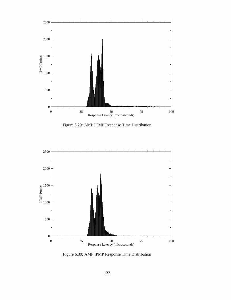
0 25 50 75 100Response Latency (microseconds)

0

500

1000

1500

2000

2500

IPM

P P

robe

s

Figure 6.29: AMP ICMP Response Time Distribution

0 25 50 75 100Response Latency (microseconds)

0

500

1000

1500

2000

2500

IPM

P P

robe

s

Figure 6.30: AMP IPMP Response Time Distribution

132

ing that the protocols were producing consistent results. These results were welcomed by

the AMP team, who believe that millisecond resolution is sufficient for RTT measurements

on the Internet. The high resolution reporting of ICMP suggests that AMP could increase

its resolution to 0.1ms, achieving an accuracy of�100�s in 87% of measurements. By dis-

abling NTP or using a more recent version of the OS on the AMP monitor with improved

clock correction capabilities this figure could be greatly improved.

The high accuracy of the passive measurements also allowed artifacts in the RTT measure-

ments due to NTP corrections of amp-kiwi’s clock drift to be seen. The time taken for

amp-kiwi to generate responses to ICMP and IPMP requests wasmeasured, showing sim-

ilar long tailed multi-modal distributions for both protocols with the majority of response

times below 50�s, making the response time only a minor contributor to RTT.

133

134

Chapter 7

Passive Characterisation of Network

Equipment

This chapter discusses the motivation for measuring the queueing behaviour of network

equipment, and practical methodologies to achieve this goal using high precision passive

measurements. Some results from differing network environments are presented.

7.1 Introduction

End to end packet delays on both LANs and WANs can often be observed to be several times

higher than the minimum delay experienced by other packets between these endpoints. If

the minimum delay approximates the propagation time plus the minimum forwarding time

through all intervening network devices, then this impliesthat packets can spend more time

in queues and buffers while in transit than they spend propagating along network links.

Packet delay variation can arise from changing routes, called route flapping, or from varia-

tions in queue occupancy at intermediate nodes due to congestion. Understanding the packet

delay variation on a path is important in correctly sizing play-out buffers for multimedia ap-

plications. Voice over IP and streaming video require buffering to reduce data loss from

late packet arrivals but simultaneously wish to minimise buffer sizes to reduce the latency

introduced by such stream reassembly.

Simulation is an important tool in understanding how trafficstreams affect each other and

135

interact with network nodes such as routers. Simulation is particularly important in under-

standing WAN behaviour, as it is often practically difficultto instrument all routers on a

long path. In order for simulation to be accurate and useful however it is important that

the simulator models the behaviour of routers and their queues accurately. This requires

that careful studies be made of queueing and forwarding behaviour in order to establish a

‘ground truth’ for such simulations at the level of individual devices.

Although the common case is that of IP routers, there are other devices that packets com-

monly pass through that may contain queues, such as layer 2 switches, Network Address

Translators, firewalls, and network accounting or analysismachines. The methodologies

presented will generally be applicable to all of these typesof devices.

7.2 Device Characterisation

7.2.1 Active Method

Active measurement may appear to be the simplest method by which to characterise the

queueing behaviour of some device. An active measurement machine connected to one

port of the device sends probe packets through it to a target machine connected to another

port, which returns response packets directly to the sourcemachine which then measures

the round trip time, see figure 7.1.

Active Source TargetDeviceUnderTest

TXRX TXRX

ProbesResponses

Figure 7.1: Active Device Characterisation

This approach suffers from the problems with all active measurement described in chapter 3

however, timing uncertainty for both transmitted and received packets at the source machine

due to scheduling and interrupt latency, as well as the unknown probe servicing delay at the

target machine. As these effects may be similar in magnitudeto the queueing delay being

136

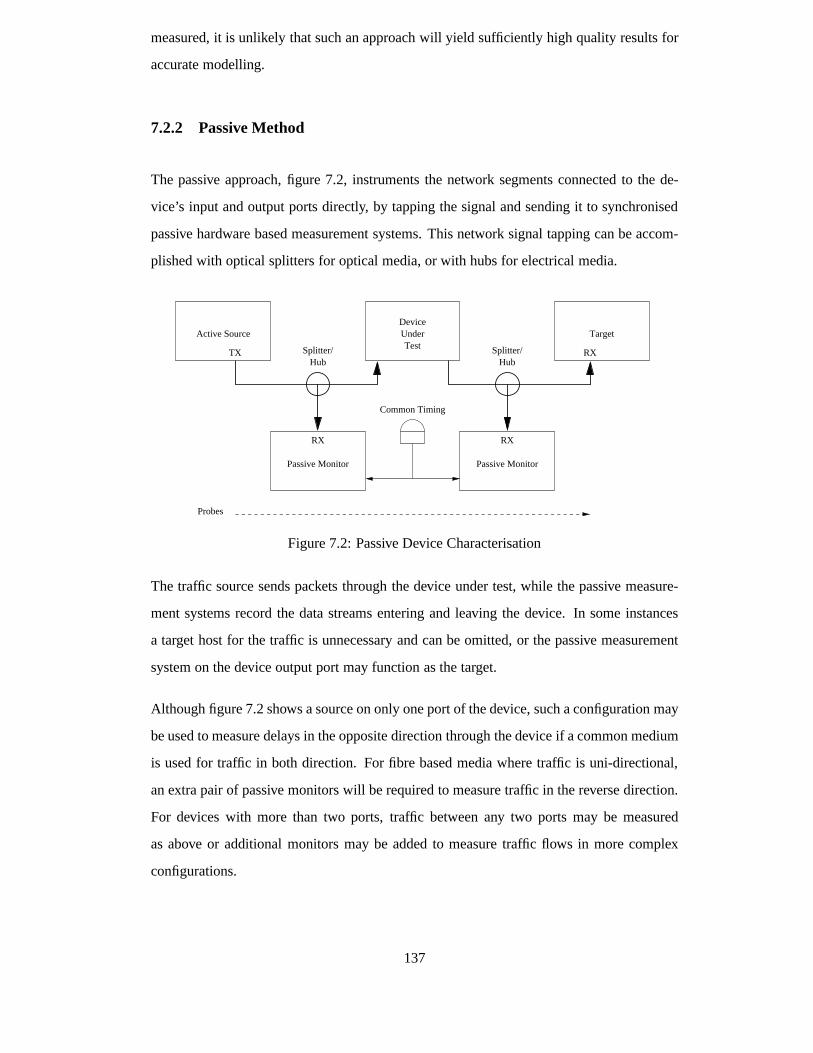
measured, it is unlikely that such an approach will yield sufficiently high quality results for

accurate modelling.

7.2.2 Passive Method

The passive approach, figure 7.2, instruments the network segments connected to the de-

vice’s input and output ports directly, by tapping the signal and sending it to synchronised

passive hardware based measurement systems. This network signal tapping can be accom-

plished with optical splitters for optical media, or with hubs for electrical media.

Splitter/Hub

Splitter/Hub

Active Source TargetDeviceUnderTest

TX RX

Passive Monitor Passive Monitor

RX RX

Probes

Common Timing

Figure 7.2: Passive Device Characterisation

The traffic source sends packets through the device under test, while the passive measure-

ment systems record the data streams entering and leaving the device. In some instances

a target host for the traffic is unnecessary and can be omitted, or the passive measurement

system on the device output port may function as the target.

Although figure 7.2 shows a source on only one port of the device, such a configuration may

be used to measure delays in the opposite direction through the device if a common medium

is used for traffic in both direction. For fibre based media where traffic is uni-directional,

an extra pair of passive monitors will be required to measuretraffic in the reverse direction.

For devices with more than two ports, traffic between any two ports may be measured

as above or additional monitors may be added to measure traffic flows in more complex

configurations.

137

7.2.3 Traffic Source

The simplest form of probe or stimulus traffic is a single synthetic traffic source. This source

can generate a periodic stream of packets at any link utilisation rate up to full line rate, or

use more sophisticated models to generate traffic streams with various statistical properties

intended to model specific protocols or to emulate a natural aggregated network load. It is

also possible to ‘replay’ a traffic stream recorded from an actual network link.

A more complex traffic source may consist of one or more sourcehosts communicating

with one or more target hosts using actual applications and protocols in order to produce a

more natural traffic load that is still controllable and repeatable.

Lastly, it is possible to install the passive measurement systems on a network device that

is installed in a production network. This has the advantageof using an actual network

load rather than a simulation, avoiding problems with potentially poor traffic models, and

simultaneously documents the actual traffic mix for furtherstudy.

Traffic on production networks however is not adjustable, rates cannot be scaled nor the

protocol mix varied, and does not provide a repeatable traffic pattern. In a production en-

vironment, the operational parameters of the device under test are also often fixed, and so

only one configuration, that being used, can be examined.

7.2.4 Measurement System Requirements

Since the effects such as delay and delay variation under study are often in the microsecond

range, unlike wide area IP studies, a hardware based approach to measurement is almost a

necessity, as the magnitude of error in a software based system may approach or exceed the

measured signal. In particular it may be very difficult to disentangle rare exceptional events

such as delay spikes caused by the device under test from unusually high interrupt latencies

in a software based measurement system due to IO or scheduling activity. An accurate

model of this exceptional behaviour is important in properly understanding and modelling

network devices.

138

7.2.5 Packet Delay and Loss Derivation

Measuring packet delay and loss with a pair of passive measurement systems as depicted

in figure 7.2 is accomplished by observing packets entering the device under test with the

source monitor, on the device’s input port, and observing packets exiting the device’s output

port with thedestination monitor.

An attempt is then made to determine which packet records from the source monitor’s trace

file correspond to packet records in the destination monitor’s trace file. Packets which can

be unambiguously identified reveal the packet delay or transit time for that packet through

the device under test. Packets which are observed in the source trace but cannot be identified

in the destination trace can be considered to have been lost.

In the simplest case, the source and destination or target networks are initially quiescent.

The passive monitors begin recording before any packets areintroduced to the source net-

work. The passive monitors cease recording after the trafficsource has been shut down, and

a reasonable period of time has elapsed to ensure that there are no packets still queued within

the device for the destination network. This delay in stopping the measurement after the last

packet has been transmitted from the source should be longerthan the largest expected delay

through the device, and serves to ensure that no packets are incorrectly recorded as missing

due to arriving on the destination network after the monitorhas stopped recording.

If after the measurement the source and destination monitors have recorded the same num-

ber of packet records, then there have been no losses within the device. Packet matching in

this case is trivial, providing packet reordering cannot occur in the device. Calculating the

delay encountered by the Nth source packet is accomplished by subtracting the time-stamp

of the Nth source packet record from the Nth destination packet record.

If fewer packets are observed on the destination network than on the source network, then

packet loss has occurred within the device. It is not sufficient to compare the number of

packets observed on the destination network with the numberof packets the traffic source

was configured to send, as output contention within the traffic source may lead to internal

packet loss at high data rates. In the presence of packet loss, the loss of individual packets

may be inferred, provided the inter-arrival time of packetsat the device is much less than

the maximum delay through the device. In the general case where the inter-arrival time of

139

packets may be much less than the maximum delay through the device, it becomes necessary

to distinguish packets explicitly based upon their content, either in the packet’s headers or

payload.

7.2.6 Packet Recognition

If the probe traffic is completely synthetic, then a simple sequence number can be placed at

a known offset within the packet, allowing the individual probe packets to be distinguished

from each other and correctly matched between the source anddestination network traces.

In order to match a packet from the source trace, the next packet in the destination trace is

read and its sequence number is compared.

If reordering cannot occur, then a higher sequence number inthe destination trace indicates

that the source packet was lost. If packet reordering can occur, then a pointer to the current

position, the first unmatched destination packet record is kept, and further destination packet

records are read from the destination trace until either thematching sequence number is

found, or a predetermined limit for the number of packets or amount of time to seek forward

is reached. This limit on the forward seeking in the destination trace would be based on a

conservative estimate of the maximum delay that could be encountered.

7.2.7 IP Id as sequence number

In the case of actual network traffic, either pre-recorded orfrom a live network link, no sim-

ple sequence number is available but it is possible to use a combination of header fields in

most cases. The IP Id header field is intended to assist in fragment reassembly, by uniquely

identifying individual packets per source address, destination address, and protocol triple

within the expected maximum life of any fragment on the Internet. These four fields to-

gether, or a hash of them, can be used to identify almost all packets uniquely within a small

window, but there are some exceptions.

Since the IP Id field is defined in the context of fragment reassembly, packets which are

retransmitted due to loss or perceived loss are permitted toreuse the Id of the original

packet. Some IP implementations, notably the Linux kernel in versions 2.3.x to 2.4.3 set

the Id field to zero for packets which also have the Don’t Fragment (DF) flag set, since

140

these packets should never be fragmented. This policy was reversed in later versions due to

problems communicating with some buggy IP implementations. Very high speed flows may

also wrap the 16-bit Id field within a window of a few seconds, causing possible confusion.

This effect is exacerbated by many implementations maintaining a global counter which is

incremented for each packet transmitted rather than a separate counter for each destination

address/protocol pair.

A further approach is to use as much information as possible about the packets in order

to reduce false matches. One possibility is to determine which fields in a packet may be

altered by the device under test, which may include link layer addresses, VLAN tags, and

the IP TTL and Header Checksum fields and mask these out, usingall of the other collected

bytes of the packet. Comparing packets directly would require many individual byte or

word-length comparisons, so it may be sufficient to generatea hash such as a CRC over the

packet to use for initial match testing.

The probability of having at least one mismatch or false CRC collision P for an-bit CRC

given a window ofr packets is approximated by equation 7.1. For a sample of 100,000

unique packets the probability of at least one collision is 0.69. These mismatches can only

be detected if a further complete comparison of the packets is performed before the match

is accepted. One approach for reducing these false matches is to use a larger CRC. With a

64-bit CRC, the probability of one or more CRC collisions in asample of 100,000 packets

is vanishingly small. P � 1� e�r(r�1)2n+1 (7.1)

In some cases multiple packets that are identical may be encountered within a short time-

frame, typically due to retransmission. Since there is no way to distinguish these packets,

unambiguous matching is not possible. In some cases it may beacceptable to use a heuris-

tic such as accepting the packet pair with the smallest time-stamp difference as matching,

otherwise all multiply matching packets must be discarded.

141

7.2.8 Revised Passive Delay Derivation Algorithm

A more efficient algorithm for packet matching was implemented in the utilitydagdelay

by Klaus Mochalski and myself which avoids repeatedly seeking within the destination

trace file and re-reading packet records. This is especiallyimportant for large trace files

that are compressed on disk and are read directly, with seek commands being emulated.

This program finds forward and reverse delays in IP traffic, dynamically building a sliding

window of records from the destination trace, and a hash table index to the window based

on partial record CRCs.

When a packet is read from the source trace, packets are read from the destination trace

and added to the queue to fill a sliding window of time about thesource packet time-stamp,

and packets in the queue that are older than the trailing end of the window are removed.

As destination packets are added to the queue, they have their hash calculated and if a

matching hash is already within the queue a destination match counter in the existing entry

is incremented, otherwise a new entry is created storing thepacket and its time-stamp.

The source packet’s hash is then calculated and looked up in the queue. If there is a matching

record, a source match counter in the packet is incremented,and the source packet’s time-

stamp is recorded. If there is no match for the source packet,a new entry is created with its

details.

As entries are removed from the tail of the queue, their matchcounters are examined. If

the packet has source and destination counts of one then there was a unique match between

the traces and the packet delay is calculated and output. If apacket has only a source

match count or destination match count of one, then it is a packet that was seen in one trace

and not the other. These unmatched packets are counted separately. If either the source

or destination counts is higher than one, then the packet’s hash was not unique within the

sliding time window, and no delay calculation is attempted.

When the ends of both files are met the queue is drained. All packets with unique matches

across both trace files within the sliding window have had their delays calculated and output,

and counts for all other cases are reported.

142

7.3 The University of Auckland Passive Measurements

The University of Auckland has collaborated with the WAND group over an extended pe-

riod, including allowing the instrumentation of their De-Militarised Zone (DMZ), the por-

tion of their network infrastructure that provides the connection between their bandwidth

provider and their internal networks. A number of anonymised IP packet header traces col-

lected over long periods have been made available to the networking community via the

WITS.

The University of Auckland buys several sets of bandwidth for different purposes such as

Internet access, and LAN Emulation and PBX services to remote campuses. A diagram of

the configuration is shown in figure 7.3. All of the bandwidth is delivered over an OC-3c

ATM circuit to an ATM switch, which collects ATM circuits from the PBXs and a router.

This router forwards packets from the ATM Internet connection from the ISP to the DMZ

Outside (dmz-o) Ethernet hub, which operates at 100Mb/s. Connected to this hub is a

computer running the FreeBSD Drawbridge firewall software,and a number of machines

that operate outside the firewall. The firewall bridges packets that pass its filtering rules to

and from the DMZ Inside (dmz-i) hub, to which the University’s LANs and other networks

connect.

Dag 3.2EDag 3.21Dag 3.21

Measurement Host PC (Linux)

ISP

Key100Mbps EthernetOC−3c ATM

Cisco 4000 Router dmz−o Hub

LANEPBX

Drawbridge 3.1 Firewall (FreeBSD)

dmz−i Hub

The Universityof Auckland

Cisco 1010 ATM switch

! PowerCOL12 345678 1236 25508012100

10

Ether 10/100

! PowerCOL12 345678 1236 25508012100

10

Ether 10/100

CiscoSystemsCiscoSystems

Figure 7.3: University of Auckland DMZ Instrumentation

Four individual points in this configuration are connected to a PC containing three Dag

cards. A single 3.2E Etherdag records packet headers from both the dmz-o and dmz-i hub

on separate ports, time-stamping them with a single DUCK. This allows the single card

to characterise both Ethernets, and to measure the delay of packets passing through the

143

firewall in both directions. The remaining two Dag 3.21s tap each direction of the the OC-

3c connection between the University ATM switch and the ISP using optical splitters. Each

direction of this link can be characterised separately, andin combination with Etherdag

measurements of the dmz-o hub, the sum of the delays experienced by packets passing

through the ATM switch and router in both directions can be measured. All of the Dag

cards’ DUCKs are connected to a single GPS receiver for synchronisation.

7.3.1 Measurement

A set of measurements was performed at the University of Auckland, recording IP headers

on all three Dag cards from all 4 network links. This measurement consisted of 19 sets

of four trace files, one for each network link, with each set typically covering a 6 hour

period. The measurement began at 18:59:16 NZST (UTC+12) on the 8th of July 2001, and

continued until 8:54:03 NZST on the 13th of July 2001.

This measurement dataset totals approximately 18GB in sizecompressed or 49,947,014,336

bytes uncompressed, and details 780,422,099 packet headers over all the four network links.

While an important and valuable resource for future study, for the analysis presented here

less data was needed, and in fact this quantity of data becomes unwieldy in all but the most

automated analysis. The behaviour of the various networks is also in no way stationary or

steady state over this length of time, with both diurnal and weekly effects present.

Two one minute time periods, table 7.1, were chosen over which to examine the delay

behaviour of the network elements. The period of one minute is much longer than both the

maximum delay times expected through the network elements,and the maximum RTT that

may be expected for IP flows into and out of the university. Thetwo periods were from

00:01 to 00:02 and from 12:01 to 12:02 NZST on Monday the 11th of July. These times

were selected so as to provide a comparison between a time at which the networks could be

expected to be at low utilisation and at high utilisation. This expectation is confirmed when

comparing the number of packet headers collected over the two periods.

144

Measure atm-in atm-out dmz-o dmz-i00:01-00:02 NZST Monday 11th July 2001

Trace size (bytes) 1307328 1349504 2504320 2506880Packet headers 20427 21086 39130 39170Traffic Volume (bytes) 10852439 10352543 17495017 17350366Average bit-rate (Mb/s) 1.45 1.38 2.33 2.31

12:01-12:02 NZST Monday 11th July 2001Trace size (bytes) 3584000 3191616 5646016 5690048Packet headers 56000 49869 88219 88907Traffic Volume (bytes) 39802152 23091358 45942180 45894004Average bit-rate (Mb/s) 5.31 3.08 6.13 6.12

Table 7.1: Summary of selected packet traces

7.3.2 Link Characteristics

The most common view of a network link is a time-series of binned data rates, typically

measured in megabits per second (Mb/s). This provides a general overview of the utilisa-

tion of the network link, including indications of the maximum and minimum data rates.

Figure 7.4 shows the network state for the night time traces,while figure 7.5 shows the

daytime state. The rise in network activity during the day isclearly visible. (Note that the

software employed in creating these graphs produces only 59points for the 60 seconds of

data captured, the last second of data is not plotted.)

Although providing an indication of the average data rates,such time series do not provide

information on the behaviour at fine time-scales, such as packet inter-arrival times. Inter-

arrival figures by themselves however neglect the effect of different sized packets, and also

fail to reference the link capacity of the network. A relatedmeasure is theInstantaneous

Bandwidth, or per-packet bandwidth.

Each packet or cell is transmitted at the full link rate for its duration on the medium, but

the packet’s contribution to the link loading can be found byincluding the inter packet time

after the packet. The instantaneous bandwidth of a packet iscalculated by dividing the size

of the packet in bits by the difference between the arrival time of the start of a packet from

the arrival time of the start of the next packet on the link. When packets are arriving back to

back, that is consuming all of the link bandwidth, then the instantaneous bandwidth for each

packet is equal to the link rate. When packets are spaced widely apart, the instantaneous

bandwidth will be proportionately smaller.

145

0 10 20 30 40 50 60Time (seconds)

0

1

2

3

4

Dat

a R

ate

(Mbp

s)

atm-inatm-outdmz-odmz-i

Figure 7.4: Link Data Rates 00:01:00 to 00:02:00

0 10 20 30 40 50 60Time (Seconds)

0

2

4

6

8

Dat

a R

ate

(Mbp

s)


Figure 7.5: Link Data Rates 12:01:00 to 12:02:00

146

Figure 7.6 shows a cumulative distribution of the instantaneous bandwidths for all of the

monitored links for the nighttime period, and figure 7.7 shows the cumulative distributions

for the daytime period. In interpreting the graphs, it can beseen that approximately 20%

of packets on both Ethernets are achieving over 80Mb/s, or are very close immediately

following a previous packet. During the night, only 6% of packets are exactly back to back,

while this rises to 11% during the day. This indicates that some packets will experience

output port contention, that is incurring delay at an outputport waiting for the Ethernet to

become quiet. At both times of day the two DMZ Ethernets show very similar behaviour,

indicating that the bridging firewall is passing most packets, and that there does not seem to

be a large difference in the amount of cross traffic on the two Ethernets.

The greatest visible feature of the ATM links is the disparity between the CDFs of the in-

coming and outgoing links. The ATM link entering the university appears to be unshaped,

that is packets may arrive with no spacing between them, thatis with an instantaneous band-

width that equals the link bandwidth of 155Mb/s. There is clearly a continuous distribution

of packet spacings to well over 100Mb/s. Despite this however previous figures indicate the

average bandwidth over one second does not exceed 8Mb/s, indicating that the bandwidth

overall is low, but that traffic can burst up to line rate without shaping when required. The

ATM link leaving Auckland however shows that 100% of packetsare limited to a bandwidth

of 4Mb/s. This is the contracted rate, and it seems likely that traffic shaping occurs at the

ATM level by means of a CBR VC.

As the traffic load increases from the night to day time measurements, the incoming link

sees a higher proportion of packets at higher bit rates. The outgoing link sees an increase

from approximately 50% of packets being throttled to 4Mb/s to around 70% of packets.

Output port contention for this link will be proportionate,and extensive buffering of packets

is expected, imposing significant delays.

7.3.3 Delay Datasets

For each time period, the four trace files were used to producetwo delay datasets, sum-

marised in table 7.2. One dataset uses the two Ethernet traces, matching packets travelling

in both directions between the measurement points, and hence through the firewall. The

second dataset measures packet delays between the dmz-o Ethernet and the ATM link. The

147

0 20 M 40 M 60 M 80 M 100 M 120 M 140 M 160 MInstantaneous Bandwidth (Mbps)

0

0.2

0.4

0.6

0.8

1

Cum

ulat

ive

Fre

quen

cy


Figure 7.6: Instantaneous Bandwidth CDF 00:01:00 to 00:02:00

0 20 M 40 M 60 M 80 M 100 M 120 M 140 M 160 MInstantaneous Bandwidth (Mbps)

0

0.2

0.4

0.6

0.8

1

Cum

ulat

ive

Fre

quen

cy

Figure 7.7: Instantaneous Bandwidth CDF 12:01:00 to 12:02:00

148

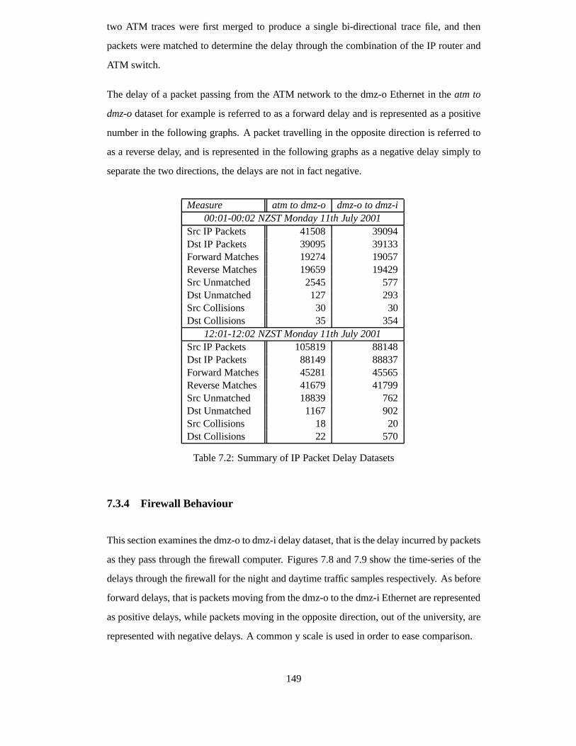
two ATM traces were first merged to produce a single bi-directional trace file, and then

packets were matched to determine the delay through the combination of the IP router and

ATM switch.

The delay of a packet passing from the ATM network to the dmz-oEthernet in theatm to

dmz-odataset for example is referred to as a forward delay and is represented as a positive

number in the following graphs. A packet travelling in the opposite direction is referred to

as a reverse delay, and is represented in the following graphs as a negative delay simply to

separate the two directions, the delays are not in fact negative.

Measure atm to dmz-o dmz-o to dmz-i00:01-00:02 NZST Monday 11th July 2001

Src IP Packets 41508 39094Dst IP Packets 39095 39133Forward Matches 19274 19057Reverse Matches 19659 19429Src Unmatched 2545 577Dst Unmatched 127 293Src Collisions 30 30Dst Collisions 35 354

12:01-12:02 NZST Monday 11th July 2001Src IP Packets 105819 88148Dst IP Packets 88149 88837Forward Matches 45281 45565Reverse Matches 41679 41799Src Unmatched 18839 762Dst Unmatched 1167 902Src Collisions 18 20Dst Collisions 22 570

Table 7.2: Summary of IP Packet Delay Datasets

7.3.4 Firewall Behaviour

This section examines the dmz-o to dmz-i delay dataset, thatis the delay incurred by packets

as they pass through the firewall computer. Figures 7.8 and 7.9 show the time-series of the

delays through the firewall for the night and daytime traffic samples respectively. As before

forward delays, that is packets moving from the dmz-o to the dmz-i Ethernet are represented

as positive delays, while packets moving in the opposite direction, out of the university, are

represented with negative delays. A common y scale is used inorder to ease comparison.

149

0 10 20 30 40 50 60Time (seconds)

-0.006

-0.004

-0.002

0

0.002

0.004

0.006

Del

ay (

seco

nds)

Figure 7.8: Packet Delays dmz-o to dmz-i 00:01:00 to 00:02:00

0 10 20 30 40 50 60Time (seconds)

-0.006

-0.004

-0.002

0

0.002

0.004

0.006

Del

ay (

seco

nds)

Figure 7.9: Packet Delays dmz-o to dmz-i 12:01:00 to 12:02:00

150

The first striking feature of both figures is how low the packetdelays are; there are no

delays higher than 6ms at any time. This indicates that the packet matching algorithm is not

generating false matches within the window with random delays, and also that the firewall

does not generate long packet delays at all. In the low traffic, nighttime time-series, there

is a central band of very low delay values that includes over 99% of the packets matched.

There is also a series of spikes in the packet delay in both directions, not exceeding 2ms.These spikes appear to have a strong periodic component, often appearing at intervals of one

second. This tends to indicate a periodic process being scheduled on the firewall computer

such as disk IO to write out logs that is temporarily interrupting the packet forwarding

process. There do not seem to be sudden periodic bursts in packet arrival at these points, and

the packets with increased delay do not seem to be unusual in any way making it unlikely

that the high delays are caused by the nature of the network traffic itself.

The higher load daytime time-series looks similar to the nighttime time-series, with the

addition of spikes out to almost 6ms. The spikes to less than 2ms still appear to be present,

so it seems likely that these larger spikes are a separate population, due to some other

periodic process that either is not present or is inactive atnight. It can be imagined that

changing load alone, or changes in the network traffic and usage patterns such as more

outgoing HTTP requests during the day may cause different logging and hence disk activity.

It is difficult to discover the exact cause without further information about the firewall rules

and logging policy.

The central band in these figures representing the bulk of thepackets seen is too dense to

understand as a time-series, figure 7.10 is a single histogram for both time periods over-

layed. Since the nighttime trace contains only half as many packets as the daytime trace,

the two histograms generally do not interfere.

The most striking feature is the three strong peaks in the reverse matches. This is however

simply due to the distribution of packet sizes. The very tallspike of low delay corresponds

to small 40-byte TCP ACK packets leaving the university while the other two spikes cor-

respond to 576 and 1500-byte packets, both common MTUs. The packet size of 576 bytes

is also common for non-TCP traffic, as this is the maximum sized packet that is guaranteed

to be carried end-to-end by IP without fragmentation, and these protocols do not support

fragmentation. The Ethernet MTU of 1500 bytes is often equalto the path MTU, as few

paths through the Internet avoid traversing an Ethernet at some point. The same distribution

151

may be seen reflected in the forward delays, but these figures appear to be spread out, and

the individual peaks are not as distinct.

The main difference between the delay distributions for thedifferent time periods seem

to be due to changes in the packet size distributions at different times of day rather than

the packet loading on the firewall software. The nighttime period shows more 576-byte

packets in the reverse direction than during the day, and a drop in both 40 and 1500-byte

packets. This appears to be due to hosts at the university serving content to users on dial-up

Internet connections with small MTUs. Forward delays show alower proportion of 1500-

byte packets at night, which may be due to less web surfing fromthe university.

With the packet delay dominated by packet size effects, it isdifficult to estimate the actual

service time of the firewall or its effective bandwidth, and whether these vary with packet

size. Figure 7.11 is a scatter-plot of packet delay on the x-axis versus packet wire length on

the y-axis. To calculate the packet wire length on Ethernet,any IP packet with a total length

less than 46 bytes is padded out to 46, then 18 is added for the MAC address, Ethernet type

field, and CRC. A further 8 is added for the preamble, and 12 forthe Inter-Frame Gap (IFG),

making the smallest possible packet wire length 84 bytes, and the largest packet wire length

1538 bytes.

This figure separates the packet size from the delay, allowing the relationship between the

two to be discerned. The two delay datasets are again overlaid with the daytime delays in

black and the nighttime delays in red. The green V shaped linedepicts the serialisation

time on a 100Mb/s Ethernet for packets of each length. The lack of any points between the

green lines indicates that no non-physical delays were found, indicating the packet matching

algorithm is not generating false matches within this region. Given the majority of packets

are represented in this small delay window, this improves confidence in the methodology.

The strong horizontal lines at certain wire packet length values correspond simply to the

common IP packet lengths of 40, 576, and 1500 bytes. Since there are so many of these

packets, their delay distributions become very dense and the individual points blur together

in this scatter-plot.

The faint vertical lines descending from the point where these common packet lengths in-

tercept their minimum delay indicate packets shorter than the packet common size that

152

-0.0002 -0.0001 0 0.0001 0.0002Delay (seconds)

0

2500

5000

7500

10000

12500

Cou

nt

12:01:00-12:02:0000:01:00-00:02:00

Figure 7.10: Packet Delay Distribution dmz-o to dmz-i

-0.0002 -0.0001 0 0.0001 0.0002Delay (seconds)

0

500

1000

1500

Wire

Pac

ket L

engt

h (B

ytes

)

Figure 7.11: Packet Delay vs. Size dmz-o to dmz-i

153

experienced a delay through the firewall equal to the delay ofthe larger packet. The most

common cause for this behaviour is where a short packet follows immediate a much longer

packet. In this case the second shorter packet cannot exit inits usual short delay time as

the tail of the longer packet is still being transmitted, effectively a case of output port con-

tention with a previous packet. Table 7.3 details the packets from a short sequence of packet

arrivals taken from the daytime trace to illustrate this point, in figure 7.12.

Packet Wire Packet Length Delay(Number) (Bytes) (Seconds)

1 1538 0.0001539592 1538 -0.0001672503 306 -0.0001674294 345 0.000045240

Table 7.3: Summary of Selected IP Packet Delays

1 2 3 4

1 2 3 4

0 0.0002 0.0004 0.0006 0.0008 0.001 0.0012 0.0014Time (seconds)

dmz-o

dmz-i

Figure 7.12: Packet Delay Sequence dmz-o to dmz-i

In this packet sequence, packet one shows the typical delay for a large 1538-byte packet

originating on the dmz-o Ethernet passing through the firewall to the dmz-i Ethernet, and

packet four shows the normal delay for a medium sized 345-byte packet. In both cases the

delay experienced by the packets through the firewall computer is equal to their serialisation

time plus a small constant. Packet two is a 1538-byte packet originating on the dmz-i

Ethernet passing through the firewall to the dmz-o Ethernet immediately followed by a

medium sized 206-byte packet. Packet two experiences its usual delay, but the small packet

following it must wait for it to be completely transmitted before it can being to be sent. This

makes the effective delay for packet three the same as the delay for the larger packet.

The line formed by the minimum delay at each packet size is well defined, and appears to

154

have an almost constant offset from the serialisation time lines. This shows that the service

time is nearly independent of packet length, and that the bandwidth of the firewall must

approach the bandwidth of the network link. On closer inspection it can be seen that the

slope of minimum delay for the reverse delay is slightly lower than the serialisation time

slope, and the bandwidth in the reverse direction can be calculated from the slope to be

approximately 90Mb/s, while the forward bandwidth slope appears to be 100Mb/s.

The line of minimum packet delay in the forward direction appears to be smeared out into

a definite band of values, compared to the sharp minima of the reverse delays. This band is

approximately 21�s wide, corresponding to 260 byte-times on a 100Mb/s Ethernet. There

are a number of possible explanations for this behaviour, although it is difficult to determine

which is the actual cause. This band is unlikely to be caused by output port contention, as

the band appears to have a constant distribution and a sharp cutoff at 260 bytes. If output

contention was the cause, the band would extend to 1500-bytetimes. Also since the two

Ethernets are similar, we would expect a similar degree of output contention in the reverse

direction.

The band may be due to varying computation times required fordifferent packets. This

would explain the lack of a similar band in the opposite direction as packets leaving the

university would face simpler filters. If this were the causehowever it might be expected that

the delay band would have some internal structure, as it is unlikely that incoming packets

are distributed evenly in any filtering attribute such as source address.

The most likely explanation would appear to be differences in the interfaces themselves.

The two NICs used on the dmz-o and dmz-i Ethernets are not identical, that is they are

different makes and models, meaning that they may have different features, and will use

different drivers. The delay band could be caused by the dmz-o NIC using a deferred inter-

rupt scheme, that is it does not interrupt the host immediately on a packet arrival but rather

waits for a fixed period for further packet arrivals in order to combine their transfer over

the PCI bus. If the dmz-i NIC does not use this mechanism, thenit will interrupt the host

immediately on packet arrivals, explaining the lack of sucha band on the reverse delays.

Differences between the two NICs could also explain the lower reverse forwarding band-

width, since if the dmz-o NIC has poor transmit performance,it may limit the output band-

width to only 90Mb/s.

155

It is difficult to distinguish the firewall’s service time from the delay distribution in fig-

ure 7.11, so the datasets are normalised by subtracting the packet serialisation time for each

matched packet, and re-plotted in figure 7.13.

From this figure we can see that the forward packet delay is independent of packet size once

serialisation time is removed, indicating that the firewallsoftware itself places no further

constraints on bandwidth. The minimum service delay in the forward direction is 17�s,apart from packets with wire lengths less than 220 bytes which may experience delays as

low as 15�s.In the reverse direction, the picture is more complex as the bandwidth in this direction is less

than than the network capacity. The average slope indicatesa forwarding rate of 90Mb/s, but

the detailed distribution actually shows two slopes. Belowapproximately 512 bytes of wire

packet length, the slope is even lower than 90Mb/s, while above this packet size the slope

is steeper, forming a knee point. Since this effect is not apparent in the forward direction

which experiences similar loading it seems unlikely that the firewall software is forming a

bottleneck. The mechanisms that the Ethernet card and driver employ in transferring packet

buffers and signalling events between the PC and the NIC are the likely root cause.

From this set of delay values normalised for the length of each packet we can construct

a histogram of the normalised delay, figure 7.14, which is directly comparable to the raw

delay histogram, figure 7.10. The delay peaks in the raw histogram corresponding to the

deserialisation times of various sized packets in the forward direction are not present in the

normalised delay histogram. It is difficult to tell if there is structure in the band of common

forward delay values, it does appear that the two separate samples, from the day and night,

show some similarities. The normalised reverse delay is still trimodal, since it is still related

to packet size even after the packet deserialisation times have been subtracted.

7.3.5 Router/Switch Behaviour

This section examines the atm to dmz-o delay dataset, that isthe delay incurred by packets

as they pass through the border router and ATM switch. The most significant feature of

these delay datasets is the relatively high amounts of delayencountered by packets leaving

the university due to the rate limited outgoing ATM connection. Figures 7.15 and 7.16 show

156

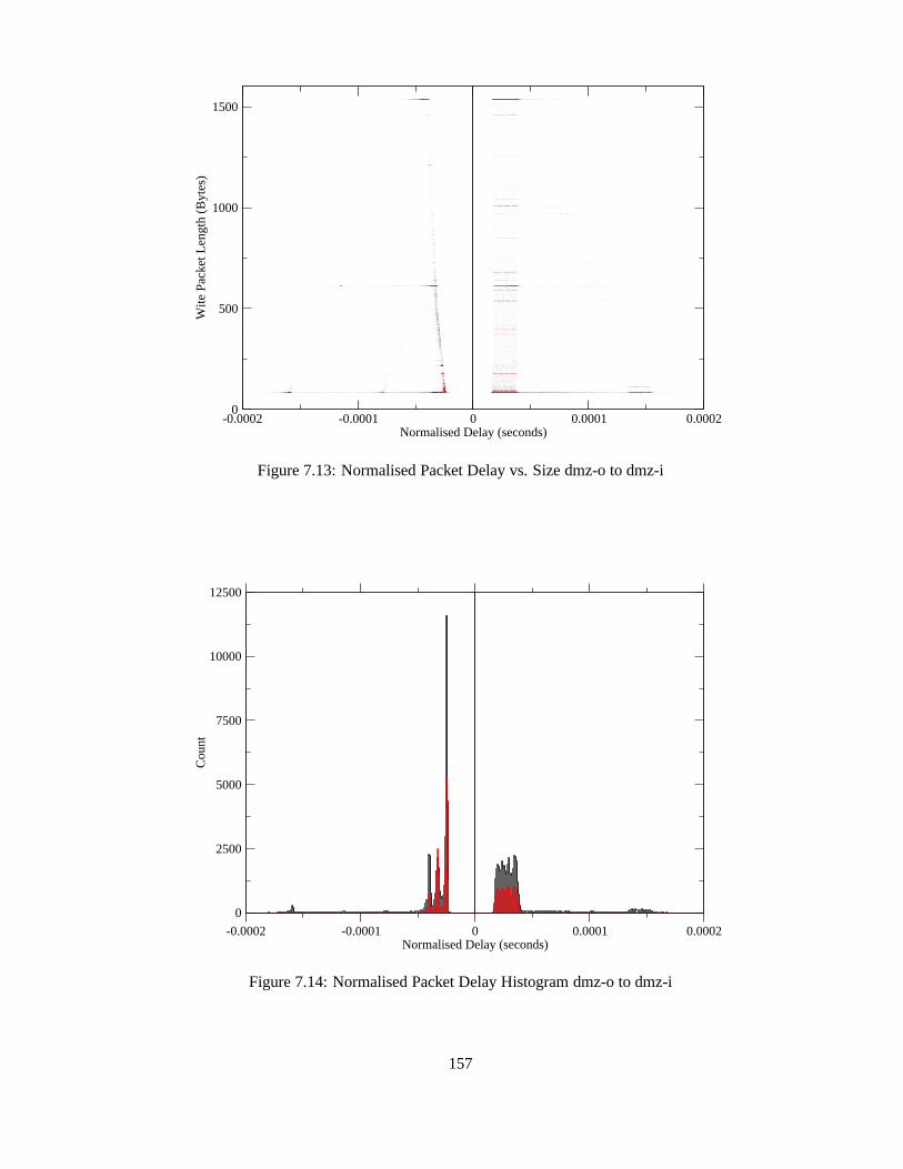
-0.0002 -0.0001 0 0.0001 0.0002Normalised Delay (seconds)

0

500

1000

1500

Wite

Pac

ket L

engt

h (B

ytes

)

Figure 7.13: Normalised Packet Delay vs. Size dmz-o to dmz-i


0

2500

5000

7500

10000

12500

Cou

nt

Figure 7.14: Normalised Packet Delay Histogram dmz-o to dmz-i

157

the delay time-series for matched unique IP packets for the night and daytime delay datasets

respectively. These two time series figures are plotted as points rather than lines to make the

spread of the points more visible. A common scale was used forcomparison, the daytime

clearly showing the longer delays and hence higher jitter due to the greater packet load.

0 10 20 30 40 50 60Time (seconds)

-0.12

-0.1

-0.08

-0.06

-0.04

-0.02

0

0.02

Del

ay (

seco

nds)

Figure 7.15: Packet Delays atm to dmz-o 00:01:00 to 00:02:00

The maximum packet delay recorded in the reverse direction was 0.116229 seconds. This

time period corresponds to 58,115 byte-times at 4Mb/s, an estimate for a lower bound on

the total buffer size. It is possible that the delay at this time is due not to simple queueing for

output, but a temporary drop in the service rate. This could be caused by internal processes

within the router, such as the scheduling of periodic background tasks, but this would affect

the forward and reverse packet forwarding rates equally.

It is possible to determine the actual size of the buffer in forwarding equipment by observing

the maximum packet delay before packets begin to be discarded, in the case where the

input bandwidth exceeds the output bandwidth. Packet loss cannot be determined however

without being able to distinguish between packets on the input interface which should be

forwarded and those which are merely cross traffic. This requires knowledge of the routing

table at the time of the measurement, which is not available in this case. It is not clear that

the maximum amount of data to be queued in this dataset exceeds the size of the buffers

causing loss, so an estimate of an upper bound for the bufferscannot be determined.

158

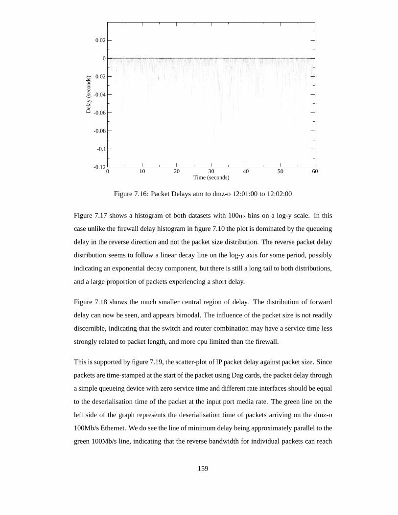
0 10 20 30 40 50 60Time (seconds)

-0.12

-0.1

-0.08

-0.06

-0.04

-0.02

0

0.02

Del

ay (

seco

nds)

Figure 7.16: Packet Delays atm to dmz-o 12:01:00 to 12:02:00

Figure 7.17 shows a histogram of both datasets with 100ns bins on a log-y scale. In this

case unlike the firewall delay histogram in figure 7.10 the plot is dominated by the queueing

delay in the reverse direction and not the packet size distribution. The reverse packet delay

distribution seems to follow a linear decay line on the log-yaxis for some period, possibly

indicating an exponential decay component, but there is still a long tail to both distributions,

and a large proportion of packets experiencing a short delay.

Figure 7.18 shows the much smaller central region of delay. The distribution of forward

delay can now be seen, and appears bimodal. The influence of the packet size is not readily

discernible, indicating that the switch and router combination may have a service time less

strongly related to packet length, and more cpu limited thanthe firewall.

This is supported by figure 7.19, the scatter-plot of IP packet delay against packet size. Since

packets are time-stamped at the start of the packet using Dagcards, the packet delay through

a simple queueing device with zero service time and different rate interfaces should be equal

to the deserialisation time of the packet at the input port media rate. The green line on the

left side of the graph represents the deserialisation time of packets arriving on the dmz-o

100Mb/s Ethernet. We do see the line of minimum delay being approximately parallel to the

green 100Mb/s line, indicating that the reverse bandwidth for individual packets can reach

159

-0.1 -0.08 -0.06 -0.04 -0.02 0Delay (seconds)

1

10

100

1000

10000

100000

Cou

nt

12:01:00-12:-2:0000:01:00-00:02:00

Figure 7.17: Packet Delay Distribution atm to dmz-o

-0.001 -0.0005 0 0.0005 0.001Delay (seconds)

0

50

100

150

200

250

300

Cou

nt

12:01:00-12:02:0000:01:00-00:02:00

Figure 7.18: Low Packet Delay Distribution atm to dmz-o

160

100Mb/s as expected. This is a rare occurrence however due tothe bandwidth limiting to

4Mb/s on the ATM circuit.

The green line on the right represents the deserialisation time for AAL5 frames on an OC-

3c circuit. The wire packet lengths are quantised since the packets are arriving on an ATM

circuit as an integer number of 53-byte ATM cells. This meansthat packets with an IP total

length of less than 32 bytes in size will fit into a single 53-byte cell, but common 40-byte

packets occupy 106 bytes on the network as opposed to 84 byteson an Ethernet. IP packets

of 1500 bytes length occupy 1538 bytes on an Ethernet, but consume 32 cells or 1696 bytes

on an ATM circuit, requiring the rescaling of the y-axis compared to previous figures.

In the forward direction we have some packets arriving at over 100Mb/s (figures 7.6 and

7.7), so we might expect to see the minimum delay slope exceed100Mb/s, however from

the graph’s slope the forwarding bandwidth is only 53Mb/s, less than either the input or

output media rates. The configuration of the router and its CPU utilisation is not known,

but it is likely that the forwarding path is CPU limited. Since the forwarding bandwidth is

still much greater than the purchased bandwidth to the ISP this is unlikely to be important

operationally.

Both forwarding directions also exhibit the banding of their minimum delay times, similar

to the forward direction of the firewall. This may indicate contention for CPU or bus re-

sources within the router or switch, or may indicate the use of deferred interrupt schemes

within the equipment. The width of the bands in both directions is approximately 115�s,compared to only 21�s for the firewall. The minimum packet delay in the reverse direction

is approximately 110�s, while the minimum packet delay in the forward direction is ap-

proximately 85�s. Both of these figures are much larger than the 17�s minimum delay for

the firewall.

The router delays are normalised by subtracting the packet deserialisation times in fig-

ure 7.20. It is again clear that the forward direction faces some forwarding bottleneck other

than the physical layers. The reverse direction although limited to only 4Mb/s on its output

link shows minimum delays consistent with a forwarding bandwidth of 100Mb/s, however

because of the bandwidth limit on the output network link it is less common for packets to

experience the minimum delay.

161

-0.0004 -0.0002 0 0.0002 0.0004Delay (seconds)

0

500

1000

1500W

ire P

acke

t Len

gth

(Byt

es)

Figure 7.19: Packet Delay vs. Size atm to dmz-o


0

500

1000

1500

Wire

Pac

ket L

engt

h (B

ytes

)

Figure 7.20: Normalised Packet Delay vs. Size atm to dmz-o

162

Figure 7.21 shows the normalised delay data as a single histogram, directly comparable with

figure 7.18. The difference in shape between the day and nightdelay distributions in the

forward direction seem to be related to the relatively lowernumber of large sized packets

arriving at the university at night rather than a change in the behaviour of the network

equipment.

-0.001 -0.0005 0 0.0005 0.0010

50

100

150

200

250

300C

ount

12:01:00-12:02:0000:01:00-00:02:00

Figure 7.21: Normalised Packet Delay Histogram atm to dmz-o

7.4 Conclusions

This chapter has demonstrated how synchronised passive measurement can be used in a

localised environment in order to measure the potentially very small delays experienced by

packets as they pass through individual pieces of network equipment.

An experiment at the University of Auckland demonstrated the measurement of packet delay

through operational network routers and fire-walls non-invasively by passively capturing

and accurately time-stamping with the existing natural packets at multiple points in the

network. An algorithm for matching unique occurrences of packets in post processing was

shown, allowing the comparison of the passive time-stamps to determine delay values.

Packet delay measurement through the border router and switch from the the internal 100Mb/s

163

Ethernet to the external ATM connection showed significant queueing delay due to rate lim-

its set on the external connection. Internal forwarding rates for the router and switch that

were significantly lower than either of the interface media rates was seen, indicating that the

router/switch combination’s forwarding performance may be CPU limited.

Measurement of delay through the firewall showed different delay characteristics between

the incoming and outgoing directions, with a mean processing delay of only 17�s per packet

independent of length, and an internal forwarding rate of atleast 90Mb/s. Incoming traffic

showed greater delay variation than outgoing traffic, whichmay be due to a greater number

of rules for incoming traffic. Periodic pauses in packet forwarding by the firewall could

be seen at one second intervals, causing packet delays of over 5ms during periods of high

traffic loads. This periodic behaviour may be due to IO activity as the firewall writes packet

logs to disk, potentially injecting long range dependence into the traffic stream.

This technique for measuring fine time scale events passively using existing natural traffic

is potentially useful in several situations. Equipment vendors when designing and testing

network equipment have access to equipment for measuring device delay behaviour, but

these typically incorporate a simplistic synthetic trafficsource. By using a passive technique

with actual network traffic, the behaviour under operational conditions can be seen, where

the full range of unusual, invalid, and corrupt packets can be experienced, along with more

natural packet inter-arrival timings.

The passive delay and bandwidth techniques can be useful operationally in networks when

diagnosing performance problems, by allowing the causes ofbandwidth bottlenecks to be

localised to specific pieces of equipment. For some streaming or real-time applications

localising the sources of delay variation across a network may be important to maximise

performance and minimise latencies.

Precise measurements of actual equipment behaviour taken from operational networks can

be used to refine the models of the equipment that are used in network simulations. Better

models of node behaviour are important for improving the fidelity of network simulations,

making the results more trustworthy and useful. Network simulations can then be used to

determine how network configurations will behave that have not been built, or estimate the

impact on the network of new protocols or applications.

164

Chapter 8

Conclusions and Future Work

8.1 Conclusions

As the speed of computer networks increase, it is necessary to continue developing systems

capable of providing high quality measurements of the fine time-scale behaviour of packets.

While some applications do not require precise timing information, for example summaris-

ing the mix of protocols or applications in use on a link, the primary utility of passive

measurement is in creating a reliable record of the packets on network links. This requires

both an accurate summary of the relevant content of all of thenetwork packets observed, and

a faithful representation of the timing of events so as to preserve the temporal relationships

within the traffic stream.

Conventional software based passive measurement systems while sufficient for low speed

links, do not scale well to high speed networks. Using a NIC for media access and time-

stamping in kernel space at interrupt time from a software clock can provide accuracies of

only tens of microseconds to the software clock, which may itself operate with considerable

skew or offset from any time standard. Attempts to constrainthe software clock’s offset to

a time standard, with NTP for example, may cause discontinuities from clock resets or high

values of skew over short periods as corrections are applied.

NICs are not an ideal platform for passive measurement when compared to the require-

ments developed here. Although it has been shown that some NICs can be modified so as to

record packet time-stamps, this requires access to technical information that is not always

165

available and success is often limited by the architecture of the hardware or resource limi-

tations. As NICs become more integrated, sometimes consisting of only a single integrated

circuit, they tend to become single purpose devices, loosing such programmable facilities.

Although NICs are commonly available for LAN technologies,commercial cards for high

speed WAN technologies may not be available, placing these links beyond the reach of NIC

based measurement.

Dedicated hardware such as the Dag cards can be built to better satisfy the specific require-

ments of passive measurement. FPGA technology can make modern designs very flexible;

extensive changes can be made to the functionality of the hardware platform even after it

has been built. This greatly lowers development costs by reducing the number of prototype

stages necessary, and avoiding the expense of designing andfabricating custom Integrated

Circuits.

Hardware based measurement systems are capable of clock resolutions of at least tens of

nanoseconds, sufficient for current gigabit class networks, and it appears likely that this

technology will scale to link speeds in the tens of gigabits range. It remains to be seen

if FPGA technology will scale to the speeds necessary for monitoring link speeds in the

hundreds of gigabits or terabit ranges. This is one avenue for future work, as link speeds

inevitably continue to increase. If network link speeds continue to rise faster than the pro-

cessing power available from host computers, further emphasis will necessarily be placed

on reducing the data-flow in the measurement session, both bycompression and by moving

packet processing operations such as filtering and flow recognition into hardware.

Passive measurement systems which precisely constrain their clock’s offset error to a global

reference signal produce network traces that not only have consistently high quality timing

internally, but their time-stamps can be compared to otherscaptured by similar remote sys-

tems. This facility enables synchronised multi-point passive measurements, the simplest

case of which is two synchronised measurement points. Two-point synchronised passive

measurement allows the One-way-Delay of packets appearingat both measurement points

to be determined. This ability can be used to calibrate or determine the error bounds in

existing One-way-Delay measurement systems by providing an independent measure of the

same delay.

The analysis of the One-way-Delay measurement system tested in this way, RIPE’s TTM

166

system, showed that the bulk of the individual One-way-Delay values reported varied less

than fifty microseconds from the passively measured wire delays. Periodic deviations from

this range to peak values over one millisecond comprise onlya small fraction of results, and

could have a number of root causes. This level of accuracy is better than expected, and more

than sufficient for the users of the system. The results of themeasurements performed by the

TTM system are used primarily in an operational sense by the participating RIPE members

to detect and record anomalous events such as route flaps or reachability problems from an

independent perspective, and not for scientific research into end-to-end IP dynamics or path

behaviour. Where only a general sense of the delay between sites or significant changes

in the base delay is needed, this level of accuracy is more than sufficient, given that the

measured delays are typically tens of milliseconds.

8.2 Future Work

Where higher accuracy in One-way-Delay measurements is desired, passive-assisted ac-

tive measurement systems where active probe packets are sent between desired points and

passively measured at both ends in order to determine One-way-Delay could be used oper-

ationally. These systems provide greater accuracy than purely active systems, at the cost of

more equipment needed at each measurement point including areference clock receiver.

Passive One-way-Delay systems could be used to measure One-way-Delay completely non-

intrusively where there is already traffic flowing between the two instrumented points. In

the case where such traffic is voluminous, it may be possible to produce very high time

resolution One-way-Delay measures. This would be useful inunderstanding One-way-

Delay variation, as events on the time-scales of the RTT, One-way-Delay, or individual

congestion events could be captured. It seems that any structure in delay variation might be

found about these fundamental time-scales.

Because hardware based passive measurement systems have higher time resolutions along

with greater accuracy than software systems it is also possible to measure very small packet

delays which may be smaller than the measurement error in software systems. This abil-

ity allows the accurate measurement of the distribution of packet delay through network

equipment such as switches, routers and fire-walls. These measurements can be used to

167

understand the behaviour and performance of these devices.They could also be used to

investigate the effects of different queueing schemes on packet streams, or as a real world

reference to create more accurate device models for use in simulation.

Multi-point passive measurement could be used to instrument an IP route end to end, al-

lowing the disentanglement of the delay contributions fromeach node and link. The ways

in which the properties of the traffic stream are changed along the path could be directly

measured, such as inter-arrival statistics or long range dependence measures. Multiple syn-

chronised passive measurement systems could also be used ina clustered configuration to

monitor all of the network ports of a core router. By measuring the delay times of all of the

packets transiting the router, models of routers could be verified and improved. It would

be possible to test if ostensibly independent packet flows through a router using separate

network interfaces become correlated through contention for potentially shared resources

such as CPU time or backplane bandwidth.

168

Appendix A

ATM Partial SAR ARM Code

This appendix provides a listing of the assembly code program executed by the StrongARM

processor on the Dag 3.x card to perform ATM partial packet reassembly and cell capture

as described inx5.5.2. The program code is formatted for the GNU Assemblergas, and

consists of the main code source file dag3atm-hash.s, and theheader file hash.h. The header

file dagarm.h is a general platform header file and is not included for brevity.

hash.h

; definitions of constants for hashing code;(1,2,3,N cell delivery out of AAL5 frames)

; ATMAAL5_END = 0x2 ; PTI bit that signals end of AAL5 PDU

; Xilinx register offsetsXHDR = 0x0 ; Location of ATM cell headerXCRC = 0x4 ; Location of ATM cell partial crcXSTATUS = 0xc8 ; Location of status registerXCD = 0xd0 ; Cell discard command register offsetXCPW = 0xd4 ; Cell copy command register offset

; Bit in status register indicating cell arrivalXDATA_AVAIL = 1

; Hash code masks etc for HASH1;; Hash1 has 17 bits hashed to give a 128k entry, 512 byte table; there are 11 bits in the check area; 4096 overflow entries are implemented, using 12 bits;

169

; Hash entry format is; : 11 check : 9 state : 12 pointer :

; state bits are:; 12 Valid - 1 if valid entry, 0 if invalid; 13 Link - 1 if link field is valid, 0 if invalid; 14 PCW - 1 if cell is to be written to host, 0 if not; 15-18 CCOUNT - 4 bit counter of cells in pdu.; Compare to Max snap. (R6)

HASH1_BASE = 0x080000 ; at 1/2 mbyteOVL_BASE = 0x078000 ; 1/2 mbyte - 32kMEM_TOP = 0x100000 ; size of memory - 1 mbyte

; 17 bit mask, VCI and lowest bit of VPIHASH1_MASK = 0x007fffcHASH1_SHIFT = 2 ; shift 2 right to word align

CHECK1_MASK = 0xffE00000 ; top 11 bits of headerLINK1_MASK = 0xfff ; lowest 12 bits; shift to 2 to get link word alignmentLINK1_SHIFT = 2; size in bytes of entries in overflow tableOVL_SIZE = 4

VALID = 0x1000 ; bit 12L_VALID = 0x2000 ; bit 13CPW1 = 0x4000 ; bit 14CCOUNT_INC = 0x8000 ; add to CCOUNT at bit 15.CCOUNT_MASK = 0x78000 ; mask the 4 CCOUNT bitsCCOUNT_CLEAR = 0x7c000 ; clear CCOUNT and CPW1; amount to shift snaplen to align with CCOUNTCCOUNT_SHIFT = 15

dag3atm-hash.s

; This program sets up a hash table entry for each new VC that; it sees. For each VC the first N cells in each AAL5 PDU are; copied over to host memory. For each MB of cells copied, the; host is interrupted. Capture continues until a stop code; is seen in a mailbox from the host.

;Register usage; r0 working register, header; r1 working register, hash entry address; r2 working register, hash entry; r3 working register; r4 Xilinx base reg; r5 Index of next free slot in overflow table base; r6 Overflow table base; r7 Link mask; r8 Loop counter

170

; r9 PCI write address; r10 Check mask; r11 hash table base; r12 Hash mask; r13 stack pointer (preserved); r14 hole base address. (link register preserved); r15 PC

; constantsDAG3 = 1.include "dagarm.h".include "hash.h"

start:stmfa sp!, {lr} ; save lr

;------------------------------------------------------------; register setup

mov r4, #XRRldr r12, =HASH1_MASKmov r11, #HASH1_BASEldr r10, =CHECK1_MASK

; This address has the hole base from drivermov r14, #0x3100ldr r9, [r14]mov r8, #0ldr r7, =LINK1_MASKmov r5, #0; zero some mailboxesstr r5, [r4, #ToHM3] ; MB write pointerstr r5, [r4, #ToHM4] ; current write pointerstr r5, [r4, #ToHM5] ; cell loss counter

;-------------------------------------------------------------; set up mmu, icache, dcache and write buffer

; bits in the command; 12 set = icache on; 11-4 must be 07; 3; 2; 1 set = mmu on. MMU must be on if dcache is on;

ldr r0, =0x107Fmcr p15, 0, r0, c1, c0, 0; write command reg

; -------------------------------------------------------------; Clear hash tables and hash overflow table,; these are contiguous in memory

; load overflow table base addressmov r0, #OVL_BASEmov r1, #0

zlp: str r1, [r0], #4cmp r0, #MEM_TOPbne zlp

; load data to remove dirty entries from dcache

171

mov r0, r11 ; load base of hash tableadd r2, r0, #16384 ; top of region being loaded

llp: ldr r1, [r0], #32 ; load a word from each dcahe lineteq r2, r0bne llp

; invalidate all dcache entriesmcr p15, 0, r0, c7, c6, 0 ; dcache invalidate command

mov r0, #0x1str r0, [r4, #ToHM2] ; 1 in ToHM2 means ready to run.

startwait:ldr r0, [r4, #ToAM2] ; check command registercmp r0, #0x1 ; 1 = runbne startwait ; keep waiting

;------------------------------------------------------------------; Reset Xilinx

str r0, [r4, #X_Reset] ; cnopnopnopnopnopnop

ldr r6, [r4, #ToAM3] ; load max snap value

mov r0, #2str r0, [r4, #ToHM2] ; signal arm running

ldr r1, [r4, #X_Status] ; clear cell drop counter

; if snaplen is zero, this is a code to capture all the cells.; Use seperate loop for efficiency.

cmp r6, #0beq fc_lp

; move snaplen so it aligns nicely with; the hash line entry counter

mov r6, r6, LSL #CCOUNT_SHIFT

;------------------------------------------------------------------; main loop

; read Xilinx header/status register; if no cell is available then the header register will read 0

lp: ldr r0, [r4, #X_Header]cmp r0, #0beq no_cell

; look for F5 / RM cells and discard.tst r0, #0x08 ; High pti bit

172

strne r0, [r4, #X_Discard_Cell] ; discardbne lp ; next cell

; compute hash table address from header

and r1, r12, r0, LSR #HASH1_SHIFTadd r1, r1, r11

; r1 has hash table entry address

get_entry:ldr r2, [r1]

; r2 has hash table entry

; Check to see if has entry is validtst r2, #VALID

beq new_entry ; go to create new entry

; compare hash table entry with header; by xor and masking. After eor only those bits; that are different in the two words will be set; the and confines the comparison to the check bits

bne no_checkeor r3, r2, r0ands r3,r3, r10

;------------------------------------------------------------------; check bits passed, so we have the right hash table entry

; see if we have to write this celltst r2, #CPW1beq cell_discard

; instruct Xilinx to write cell to PCIstr r9, [r4, #X_Copy_Cell]

; increment PCI write pointeradd r9, r9, #64

; increment in-pdu countadd r2, r2, #CCOUNT_INC ; add 1 at bit 15and r3, r2, #CCOUNT_MASK; mask in countcmp r3, r6 ; do compare to max capture

; if at max, clear count and copy bit in R2.biceq r2, r2, #CCOUNT_CLEAR

; ALL5 write test; at this stage the CPW bit must be set in the hash entry.; If the cell is not the last on in the PDU then this bit; must be cleared and the now dirty hash entry written back

; If this cell has end marker, set copy bit and clear CCOUNTtst r0, #AAL5_ENDorrne r2, r2, #CPW1bicne r2, r2, #CCOUNT_MASK

; always write back the modified hash entrystr r2, [r1]

173

; this case is finished. Do end of loop tests

add r8, r8, #1 ; increment cell counterldr r0, =0xfffff ; check for MB boundarytst r9, r0bne lp ; if not boundary, next cellstr r9, [r4, #ToHM3] ; store address in mailbox3mov r0, #0x4str r0, [r4, #ToHDB] ; interrupt PC

ldr r1, [r14] ; load hole base addressldr r0, [r14, #4] ; load hole top addresscmp r9, r0 ; check for PC buffer fullmoveq r9, r1 ; start from base again

ldr r0, [r4, #ToAM2] ; check command registercmp r0, #0x2 ; 2 = finishbne lp ; next cellb finish

;------------------------------------------------------------------no_cell:; This is what we do when there is no cell available

; report current address in host memorystr r9, [r4, #ToHM4]ldr r0, [r4, #X_Status]str r0, [r4, #ToHM5] ; report cell lossldr r0, [r4, #ToAM2] ; check command registercmp r0, #0x2 ; 2 = finishbne lp ; next cellb finish

;------------------------------------------------------------------cell_discard:; not writing this cell, so throw it away

str r9, [r4, #X_Discard_Cell]

; ALL5 write test; At this stage the CPW bit must be zero in the hash entry.; If this cell is the last on in the PDU then this bit must; be set and the now dirty hash entry written back

tst r0, #AAL5_ENDorrne r2, r2, #CPW1

; write back the modified hash entrystrne r2, [r1]

; this case is finished. Do end of loop tests

add r8, r8, #1 ; increment cell counterb lp

;------------------------------------------------------------------no_check:

174

; check bits failed, so try to follow links

; check if link is validtst r2, #L_VALIDbeq make_link

; link is valid , so compute new hash entry address; and branch back for checks

mov r3, #OVL_BASEand r1, r2, r7 ; mask link bits

; add in overflow table baseadd r1, r3, r1, LSL #LINK1_SHIFT

; go back to check this entryb get_entry

;------------------------------------------------------------------make_link:; Link in an overflow hash table entry to existing entry

mov r3, #OVL_BASEbic r2, r2, r7 ; make sure link bits are clearorr r2, r2, r5 ; Or in link destination indexorr r2, r2, #L_VALID ; set link valid bitstr r2,[r1] ; replace the hash table entry

; calculate address to put new entryadd r1, r3, r5, lsl #LINK1_SHIFT

; move pointer to next empty overflow slotadd r5, r5, #OVL_SIZE

; drop through to new_entry

;------------------------------------------------------------------new_entry:; create new table entry, from header stored in R0; and place in [r1]

; throw away the cell as we don’t need itstr r9, [r4, #X_Discard_Cell]and r2, r0, r10 ; clear all except check bitsorr r2, r2, #VALID ; set VALID flag

;; ALL5 write test

; at this stage the CPW bit is zero in the hash entry.; If this cell is the last on in the PDU then this bit must be set.

tst r0, #AAL5_ENDorrne r2, r2, #CPW1

; write back the modified hash entrystr r2, [r1]

; this case is finished.add r8, r8, #1 ; increment cell counterb lp ; back to top for next cell

;------------------------------------------------------------------finish:

175

; check cell drop counterldr r10, [r4, #X_Status]

; load data to remove dirty entries from dcachemov r0, r11 ; load base of hash tableadd r2, r0, #32768 ; top of region being loaded

llp2: ldr r1, [r0], #32 ; load a word from each dcache lineteq r2, r0bne llp2

; invalidate all dcache entries

mcr p15, 0, r0, c7, c6, 0 ; dcache invalidate command; disable cache and WB.

ldr r0, =0x1071mcr p15, 0, r0, c1, c0, 0 ; write command reg

mov r0, #0x3str r0, [r4, #ToHM2] ; 3 in ToHM2 means stopped.ldmfa sp!, {lr} ; restore lrmov pc, lr

;------------------------------------------------------------------; This is the loop for full capture

fc_lp: ldr r0, [r4, #X_Header]cmp r0, #0beq fc_no_cell

; Always write cell; instruct Xilinx to write cell to PCI

str r9, [r4, #X_Copy_Cell]; increment PCI write pointer

add r9, r9, #64add r8, r8, #1 ; increment cell counter

ldr r0, =0xfffff ; check for MB boundarytst r9, r0bne fc_lp ; if not boundary, next cellstr r9, [r4, #ToHM3] ; store address in mailbox3mov r0, #0x4str r0, [r4, #ToHDB] ; interrupt PC

ldr r0, [r14, #4] ; load hole top addresscmp r9, r0 ; check for PC buffer fullldreq r1, [r14] ; load hole base addressmoveq r9, r1 ; start from base again

ldr r0, [r4, #ToAM2] ; check command registercmp r0, #0x2 ; 2 = finishbne fc_lp ; next cellb finish

;------------------------------------------------------------------fc_no_cell:

176

; This is what we do when there is no cell available

; report current address in host memorystr r9, [r4, #ToHM4]ldr r0, [r4, #X_Status]str r0, [r4, #ToHM5] ; report cell lossldr r0, [r4, #ToAM2] ; check command registercmp r0, #0x2 ; 2 = finishbne fc_lp ; next cellb finish

177

178

Appendix B

AMP Monitors

This appendix lists the AMP monitors participating in the experiment detailed inx6.5.

AMP Name Site Location

amp-alaska University of Alaska Fairbanks, AK

amp-arizona University of Arizona Tucson, AZ

amp-asu Arizona State University Phoenix, AZ

amp-bcm Baylor College of Medicine Houston, TX

amp-bu Boston University Boston, MA

amp-buffalo State University of New York at Buffalo Buffalo, NY

amp-c3ardnoc CANARIE Inc Ottawa, Canada

amp-caltech California Institute of Technology Pasadena,CA

amp-clemson Clemson University Anderson, SC

amp-colostate Colorado State University Fort Collins, CO

amp-columbia Columbia University New York, NY

amp-cornell Cornell University Ithaca, NY

amp-csu-sb California State University San Bernardino Marshall, CA

amp-csupomona California State University Pomona Walnut,CA

amp-cwru Case Western Reserve University Cleveland, OH

amp-dartmouth Dartmouth College Hanover, NH

amp-duke Duke University Durham, NC

amp-emory Emory University Atlanta GA

amp-fiu Florida International University Miami, FL

179

amp-fnal Fermilab Batavia, IL

amp-fsu Florida State University Tallahassee, FL

amp-gatech Georgia Institute of Technology Atlanta, GA

amp-georgetown Georgetown University Washington, DC

amp-gmu George Mason University Fairfax, VA

amp-gsfc NASA Goddard Space Flight Center Greenbelt, MD

amp-harv Harvard University Cambridge, MA

amp-hawaii University of Hawaii Honolulu, HI

amp-iastate Iowa State University Ames, IA

amp-indianai Indiana University Bloomington, IN

amp-jhu Johns Hopkins University Baltimore, MD

amp-jpl NASA Jet Propulsion Laboratory Pasadena, CA

amp-kiwi University of Waikato Hamilton, New Zealand

amp-korea System Engineering Research Institute Seoul, Korea

amp-ksu Kansas State University Manhattan, KS

amp-lbnl Lawrence Berkeley National Laboratory Berkeley,CA

amp-memphis Memphis State University Memphis, TN

amp-miami University of Miami Miami, FL

amp-missouri University of Missouri-Columbia Columbia, MO

amp-mit Massachusetts Institute of Technology Cambridge,MA

amp-montana Montana State University Bozeman, MT

amp-msstate Mississippi State University Mississippi State, MS

amp-msu Michigan State University East Lansing, MI

amp-mtu Michigan Technological University Houghton, MI

amp-ncar National Center for Atmospheric Research Boulder, CO

amp-ncren North Carolina Research and Education Network Durham, NC

amp-ncsa National Center for Supercomputing ApplicationsChampaign, IL

amp-ncsa-dca National Center for Supercomputing Applications Arlington, VA

amp-ncsu North Carolina State University Raleigh, NC

amp-ndsu North Dakota State University Fargo, ND

amp-nmsu New Mexico State University Las Cruces, NM

amp-nwu Northwestern University Evanston, IL

amp-nysernet NYSERNet Syracuse, NY

180

amp-odu Old Dominion University Norfolk, VA

amp-ohio-state Ohio State University Columbus, OH

amp-okstate Oklahoma State University Stillwater, Oklahoma

amp-orst Oregon State University Corvallis OR

amp-ou University of Oklahoma Norman, OK

amp-princeton Princeton University Princeton, NJ

amp-psc Pittsburgh Supercomputing Center Pittsburgh, PA

amp-psu Pennsylvania State University University Park, PA

amp-rice Rice University Houston, TX

amp-sdsc San Diego Supercomputer Center San Diego, CA

amp-sdsmt South Dakota School of Mines & Technology Rapid City, SD

amp-sdsu San Diego State University San Diego, CA

amp-sdwr San Diego Supercomputer Center San Diego, CA

amp-slac Stanford Linear Accelerator Center Stanford, CA

amp-smu Southern Methodist University Dallas, TX

amp-stanford Stanford University Stanford, CA

amp-startap Star Tap Arlington Heights, IL

amp-thor University of Trondheim Trondheim, Norway

amp-ua University of Alabama Tuscaloosa, AL

amp-uab University of Alabama at Birmingham Birmingham, AL

amp-uah University of Alabama in Huntsville Huntsville, AL

amp-uc University of Cincinnati Cincinnati, OH

amp-ucb University of California, Berkeley Berkeley, CA

amp-ucboulder University of Colorado Boulder, CO

amp-ucf University of Central Florida Orlando, FL

amp-uci University of California, Irvine Irvine, CA

amp-ucla University of California, Los Angeles Los Angeles, CA

amp-uconn University of Connecticut Storrs, CT

amp-ucsc University of California, Santa Cruz Santa Cruz, CA

amp-ucsd University of California, San Diego La Jolla, CA

amp-udel University of Delaware Newark, DE

amp-ufl University of Florida Gainesville, FL

amp-uga University of Georgia Athens, GA

181

amp-uic University of Illinois at Chicago Chicago, IL

amp-uiowa University of Iowa Iowa City, IA

amp-uiuc University of Illinois at Urbana-Champaign Urbana, IL

amp-ukans University of Kansas Lawrence, KS

amp-umass University of Massachusetts Amherst, MA

amp-umbc University of Maryland, Baltimore County Baltimore, MD

amp-umd University of Maryland College Park, MD

amp-umich University of Michigan Ann Arbor, MI

amp-unc-ch University of North Carolina Chapel Hill, NC

amp-unm University of New Mexico Albuquerque, NM

amp-uoregon University of Oregon Eugene, OR

amp-upenn University of Pennsylvania Philadelphia, PA

amp-uroch University of Rochester Rochester, NY

amp-usf University of South Florida Tampa, FL

amp-utah University of Utah Salt Lake City, UT

amp-utexas University of Texas Austin, TX

amp-utk University of Tennessee Memphis, TN

amp-uva University of Virginia Charlottesville, VA

amp-uvm University of Vermont Burlington, VT

amp-uwashington University of Washington Seattle, WA

amp-uwm University of Wisconsin-Milwaukee Milwaukee, WI

amp-uwyo University of Wyoming Laramie, WY

amp-vanderbilt Vanderbilt University Nashville, TN

amp-vt Virginia Polytechnic Institute and State University Blacksburg, VA

amp-wayne Wayne State University Detroit, MI

amp-wisc University of Wisconsin-Madison Madison, WI

amp-wpi Worcester Polytechnic Institute Worcester, MA

amp-wsu Washington State University Pullman, WA

amp-wustl Washington University St. Louis, MO

amp-wvu West Virginia University Morgantown, WV

amp-yale Yale University New Haven, CT

182

Bibliography

Abry, P., Flandrin, P., Taqqu, M. and Veitch, D. [2000]. Self-similarity and long-range

dependence through the wavelet lens. In P. Doukhan, G. Oppenheim and M. S. Taqqu

(Eds.),Long-range Dependence: Theory and Applications. Birkhauser.

Acharya, M. and Bhalla, B. [1994]. A flow model for computer network traffic using

real-time measurements. InSecond International Conference on Telecommunications

Systems, Modeling and Analysis. Nashville, TN.

Acharya, M., Newman-Wolfe, R., Latchman, H., Chow, R. and Bhalla, B. [1992].

Real-time hierarchical traffic characterization of a campus area network. In

Proceedings of the Sixth International Conference on Modeling Techniques and Tools

for Computer Performance Evaluation. University of Florida.

Almes, G., Kalidindi, S. and Zekauskas, M. [1999]. A one-waydelay metric for IPPM.

Technical Report RFC2679, IETF.

Apisdorf, J., Claffy, K., Thompson, K. and Wilder, R. [1994]. OC3MON: Flexible,

affordable, high performance statistics collection. InProceedings of th Tenth USENIX

System Administrarion Conference (LISA X)(pp. 97–112). Chicago, IL.

Apptel [1999].POINT (PCI Optical Interface Network Transceiver) Hardware Design

Manual(0.70 Ed.). Lisle, IL: Applied Telecom, Inc.

http://www.apptel.com/pdf/pointmanv70.pdf.

Bailey, M. L., Gopal, B., Pangels, M. A. and Peterson, L. L. [1994]. PATHFINDER: A

pattern-based packet classifier. InProceedings of the First USENIX Symposium on

Operating Systems Design and Implementation(pp. 115–123). Monterey, CA.

183

Begel, A., McCanne, S. and Graham, S. L. [1999]. BPF+: exploiting global data-flow

optimization in a generalized packet filter architecture. In Proceedings of ACM

SIGCOMM ’99 conference on Applications, technologies, architectures, and

protocols for computer communications(pp. 123–134). Cambridge, MA.

Braden, R. [1989]. Requirements for internet hosts – communication layers. Technical

Report RFC1122, IETF.

Braden, R. T. and DeSchon, A. [1998]. NNStat: Internet statistics collection package,

introduction and user guide. Technical report, ISI, USC.

Brownlee, N. [1999a].NeTraMet & NeMaC Reference Manual v4.3. The University of

Auckland, Auckland, New Zealand: Information Technology Systems & Services.

Brownlee, N. [1999b]. SRL: A language for describing trafficflows and specifying actions

for flow groups. Technical Report RFC2723, IETF.

Brownlee, N., Mills, C. and Ruth, G. [1999]. Traffic flow measurement: Architecture.

Technical Report RFC2722, IETF.

Cisco [2000]. Netflow services and applications. Technicalreport, Cisco Systems, Inc.

http://www.cisco.com/warp/public/cc/pd/iosw/ioft/neflct/tech/nappswp.htm.

Claffy, K. [1994]. Internet traffic characterization. PhD thesis, UCSD, San Diego, CA.

Claffy, K. C., Polyzos, G. C. and Braun, H.-W. [1993a]. Application of sampling

methodologies to network traffic characterization. InProceedings of ACM

SIGCOMM ’93. ftp://oceana.nlanr.net/papers/sigcomm.sampling.ps.gz.

Claffy, K. C., Polyzos, G. C. and Braun, H.-W. [1993b]. Traffic characteristics of the T1

NSFNET backbone. InProc. Joint Conference of the IEEE Computer and

Communications Societies (INFOCOM’93)(pp. 885–892). San Francisco, CA.

Curtis, J. P., Cleary, J. G., McGregor, A. J. and Pearson, M. W. [2000]. Measurement of

voice over IP traffic. InThe First Passive and Active Measurement Workshop,

PAM2000. http://www/pam2000/pdfpapers/pam2000c.pdf.

DEC, Intel and Xerox [1982]. Ethernet local area network specification version 2.0. DEC

Part Number: AA-K759B-TK.

184

Demichelis, C. and Chimento, P. [2001]. Instantaneous packet delay variation metric for

IPPM. Technical Report draft-ietf-ippm-ipdv-07.txt, IETF.

Deng, X. [1999]. Short term behaviour of ping measurements.Master’s thesis, The

University of Waikato.

http://wand.cs.waikato.ac.nz/wand/publications/xingthesis.ps.gz.

Engler, D. R. and Kaashoek, M. F. [1996]. DPF: Fast, flexible message demultiplexing

using dynamic code generation. InProceedings of ACM SIGCOMM ’96(pp. 53–59).

Stanford, CA.

Graham, I. and Cleary, J. [1996]. Cell level measurements ofATM-25 traffic. Technical

report, The University of Waikato.

http://wand.cs.waikato.ac.nz/wand/publications/CLMATMT.ps.gz.

Graham, I., Pearson, M., Martens, J., Donnelly, S. and Cleary, J. G. [1997]. A remote atm

network monitoring system. Technical report, The University of Waikato.

http://www.cs.waikato.ac.nz/Pub/Html/ATMNetMonSysPaper/ATMMonSyst.html.

Graham, I. D., Donnelly, S. F., Martin, S., Martens, J. and Cleary, J. G. [1998].

Nonintrusive and accurate measurement of unidirectional delay and delay variation

on the internet. INET’98 Online Proceedings.

http://www.isoc.org/inet98/proceedings/6g/6g2.htm.

Jacobson, V. [1989].traceroute(8). Lawrence Berkeley National Laboratory. available via

anonymous ftp: ftp://ftp.ee.lbl.gov/traceroute.tar.gz.

Jain, R. and Routhier, S. A. [1986]. Packet trains — measurement and a new model for

computer network traffic.IEEE Journal on Selected Areas in Communications, 4(6),

986–995.

Joyce, S. K. [2000]. Traffic on the internet - a study of internet games. Master’s thesis, The

University of Waikato. Honours Project

http://wand.cs.waikato.ac.nz/wand/publications/sarah-420.pdf.

Kalidindi, S. and Zekauskas, M. J. [1999]. Surveyor: An infrastructure for internet

performance measurements. INET’99 Online Proceedings.

http://www.isoc.org/inet99/proceedings/4h/4h2.htm.

185

Kamp, P.-H. [1998]. Raw data: Interrupt latency measurement. Technical report, The

FreeBSD Project.

Keys, K., Moore, D., Koga, R., Lagache, E., Tesch, M. and Claffy, K. [2001]. The

architecture of CoralReef: an internet traffic monitoring software suite. In

Proceedings of PAM2001 - A workshop on Passive and Active Measurements.

Amsterdam, Netherlands.

Kleen, A. [1999].packet(7); Linux Programmer’s Manual.

Mao, G. and Habibi, D. [2000]. Loss performance analysis forheterogeneous on-off

sources. http://www-soem.ecu.edu.au/ gmao/Lossperformanceanalysis.ps.gz.

Martin, H. S., McGregor, A. J. and Cleary, J. G. [2000]. Analysis of internet delay times.

In The First Passive and Active Measurement Workshop, PAM2000.

http://www.cs.waikato.ac.nz/pam2000/pdfpapers/P033.pdf.

McCanne, S. and Jacobson, V. [1993]. The BSD packet filter: A new architecture for

user-level packet capture. InProceedings of the 1993 winter USENIX technical

conference(pp. 259–269). San Diego, CA.

McCanne, S., Leres, C. and Jacobson, V. [1991].tcpdump. Berkeley, CA: Lawrence

Berkeley Laboratory. available from http://www.tcpdump.org/.

McCanne, S., Leres, C. and Jacobson, V. [1994].libpcap. Berkeley, CA: Lawrence

Berkeley Laboratory. available from http://www.tcpdump.org/.

McCloghrie, K. and Rose, M. [1991]. Management informationbase for network

management of TCP/IP-based internets: MIB-II. Technical Report RFC1213, IETF.

Internet Standard STD0017.

McGregor, A. [1998]. IP measurement protocol (IPMP). AMP Website.

http://amp.nlanr.net/AMP/IPMP/ipmp.html.

McGregor, A. and Braun, H.-W. [2000]. Balancing cost and utility in active monitoring:

The AMP example.Inet2000.

http://www.isoc.org/inet2000/cdproceedings/1d/1d3.htm.

186

Micheel, J., Graham, I. and Brownlee, N. [2001]. The auckland data set: an access link

observed. InProceedings of the 14th ITC Specialists Seminar on Access Networks

and Systems. http://wand.cs.waikato.ac.nz/wand/publications/barcelona-2001.pdf.

Mills, D. L. [1992]. Network time protocol (version 3). Technical Report RFC1305, IETF.

Mogul, J. C., Raschid, R. F. and Accetta, M. J. [1987]. The packet filter: And efficient

mechanism for user-level network code. InProceedings of the 11th Symposium on

Operating Systems Principles(pp. 39–51). Austin TX.

Muuss, M. [1983].ping(8); FreeBSD System Manager’s Manual. US Army Ballistics

Research Laboratory.

Pasztor, A. and Veitch, D. [2001]. A precision infrastructure for active probing. In

Proceedings of PAM2001 - A workshop on Passive and Active Measurements.

Amsterdam, Netherlands.

Paxson, V., Almes, G., Mahdavi, J. and Mathis, M. [1998]. Framework for IP performance

metrics. Technical Report RFC2330, IETF.

Postel, J. [1981]. Internet control message protocol. Technical Report RFC792, IETF.

Ribero, V., Coates, M., Riedi, R., Sarvotham, S., Hendricks, B. and Baraniuk, R. [2000].

Multifractal cross-traffic estimation. InProceedings of the 13th ITC Specialist

Seminar on IP Traffic Measurement, Modelling and Management.

http://www.dsp.rice.edu/publications/pub/itc00crosstraffic.ps.gz.

Rivest, R. [1992a]. The md4 message-digest algorithm. Technical Report RFC1320, IETF.

Rivest, R. [1992b]. The md5 message-digest algorithm. Technical Report RFC1321, IETF.

Roux, S., Veitch, D., Abry, P., Huang, L. and Flandrin, P. [2001]. Statistical scaling

analysis of TCP/IP data using cascades. InProceedings of the International

Conference on Acoustics, Speech, and Signal Processing.

http://moat.nlanr.net/Traces/Kiwitraces/icassp01.ps.

Sun [1990].NIT(4P); SunOS 4.1.1 Reference Manual. Mountain View, CA: Sun

Microsystems Inc. Part Number 800-5480-10.

Tree, P. [2000].Dag 3 Installation Guide. The University of Waikato.

http://dag.cs.waikato.ac.nz/dag/docs/digv2.1.pdf.

187

Trimble [1999].Palisade NTP Synchronization Kit User Guide. Trimble Navigation

Limited Timing and Synchronization Group. Part Number 39139-00.

Uijterwaal, H. and Kolkman, O. [1997]. Internet delay measurements using test traffic.

Technical Report RIPE-158, RIPE NCC.

Waldbusser, S. [1997]. Remote network monitoring management information base version

2 using SMIv2. Technical Report RFC2021, IETF.

Waldbusser, S. [2000]. Remote network monitoring management information base.

Technical Report RFC2819, IETF. Internet Standard STD0059.

Yuhara, M., Bershad, B., Maeda, C., Eliot, J. and Moss, B. [1994]. Efficient packet

demultiplexing for multiple endpoints and large messages.In Proceedings of the

1994 winter USENIX technical conference(pp. 153–165). San Francisco, CA.

Ziedins, I. [2000]. On the output process from a finite bufferwith long range dependent

input. http://wand.cs.waikato.ac.nz/wand/publications/ziedins2000.ps.gz.

188

Documents

High Precision Timing in Passive Measurements of Data Networksdjm202/pdf/papers/stephen-thesis.pdf · 2009-08-28 · High Precision Timing in Passive Measurements of Data Networks