High Temperature Seismic Monitoring for Enhanced Geothermal Systems

High Temperature Seismic Monitoring for

Enhanced Geothermal Systems

Implementing a Control Feedback Loop to a Prototype Tool by Sandia National Laboratories

Panit Howard

Thesis submitted to the faculty of the Virginia Polytechnic Institute and State University

in partial fulfillment of the requirements for the degree of

Masters of Science

in

Mechanical Engineering

Dennis Hong

Alfred L. Wicks

Frank Maldonado

ii

Geothermal energy can make an important contribution to the U.S. energy portfolio. Production

areas require seismic monitoring tools to develop and monitor production capability. This paper

describes modifications made to a prototypical seismic tool to implement improvements that were

identified during previous tool applications. These modifications included changing the motor

required for mechanical coupling the tool to a bore-hole wall. Additionally, development of a closed-

loop process control utilized feedback from the contact force between the coupling arm and bore-hole

wall. Employing a feedback circuit automates the tool deployment/anchoring process and reduces

reliance on the operator at the surface. The tool components were tested under high temperatures and

an integrated system tool test demonstrated successful tool operations.

High Temperature Seismic Monitoring for Enhanced Geothermal Systems

Implementing a Control Feedback Loop to a Prototype Tool by Sandia National Laboratories

Panit Howard

Abstract

iii

Acknowledgements

This thesis would not have been possible without the help and support of the kind people around

me.

Above all, I would like to thank my parents and sister who have given me their unwavering

support and love throughout my academic and professional career. I want to thank my manager

Dr. Christi Leigh, who strongly influenced my decision to further my education and her

dedicated support to my academic and professional development. I wish to thank Doug

Blankenship and Frank Maldonado for providing a project where I was able to contribute to the

advancement of geothermal system monitoring. Additionally, I need to extend a big thanks to

the rest of the team in the Geothermal Energy Department at Sandia National Laboratories. They

brought me in, treated me like one of their own, and provided the support necessary for me to

complete my project on time.

This thesis would not have been possible without the support and patience of my advisors Dr.

Dennis Hong and Dr. Alfred L. Wicks, granting me the opportunity to work on a project of my

choosing. I’d like to recognize Cathy Hill, the Mechanical Engineering Department chief

coordinator and administrative assistant, whom assisted me by obtaining signatures and

submitting the required forms enabling my success in meeting the administrative requirements

associated with submitting and defending this thesis.

I acknowledge Sandia National Laboratories for their financial support, allowing me to focus on

my education and sponsoring this work. Lastly, I want to thank my all my friends who were

supportive while I was at school.

Sandia National Laboratories is a multi-program laboratory managed and

operated by Sandia Corporation, a wholly owned subsidiary of Lockheed

Martin Corporation, for the U.S. Department of Energy’s National Nuclear

Security Administration under contract DE-AC04-94AL85000.

iv

TABLE OF CONTENTS

List of Figures .............................................................................................................................. vii

List of Tables .............................................................................................................................. viii

Chapter 1. Introduction ............................................................................................................. 1

1.1 Motivation Behind Research ............................................................................................ 2

1.2 Scope ................................................................................................................................ 2

Chapter 2. Literature Review ................................................................................................... 3

2.1 Enhanced Geothermal Systems ........................................................................................ 3

2.2 Geothermal Stimulation Processes ................................................................................... 4

2.2.1 Hydraulic Fracturing ................................................................................................ 4

2.2.2 Basics of Hydroshearing ........................................................................................... 6

2.3 Seismic Monitoring .......................................................................................................... 6

2.4 Current Technologies ....................................................................................................... 8

Chapter 3. Requirements, Constraints, and System Design .................................................. 8

3.1 Environmental Requirements and Constraints ................................................................. 8

3.1.1 Physical ..................................................................................................................... 9

3.1.2 Chemical ................................................................................................................... 9

3.2 System Conceptual Design ............................................................................................. 10

Chapter 4. System Design Specifications ............................................................................... 12

4.1 Conventional Technology .............................................................................................. 12

4.2 High Temperature Adaptations ...................................................................................... 12

4.2.1 Mechanical System Specifications .......................................................................... 12

4.2.2 Electrical System ..................................................................................................... 13

4.2.3 Operational System ................................................................................................. 13

Chapter 5. Seismic Monitoring System Design Modifications ............................................. 13

5.1 Mechanical System Design ............................................................................................ 14

5.2 Electrical Design ............................................................................................................ 14

5.3 Software Design ............................................................................................................. 16

Chapter 6. Component and System Testing Sequence Design ............................................. 17

v

Chapter 7. Phase 1: Component Testing................................................................................ 18

7.1 Supporting Equipment.................................................................................................... 18

7.1.1 Physical Support Equipment ................................................................................... 18

7.1.2 Diagnostic Support Equipment ............................................................................... 19

7.2 High Temperature Motor Test ........................................................................................ 20

7.2.1 Procedure for Testing Motor .................................................................................. 21

7.2.2 Results ..................................................................................................................... 22

7.2.3 Performance/Conclusions ....................................................................................... 23

7.3 High Temperature Current Sensor Test ......................................................................... 24

7.3.1 Procedure for Testing Current Sensing .................................................................. 24

7.3.2 Results ..................................................................................................................... 25

7.3.3 Performance/Conclusions ....................................................................................... 25

Chapter 8. Phase 2: Electro-Mechanical System Test .......................................................... 26

8.1 Initial Electro-Mechanical System Test ......................................................................... 26

8.1.1 Support Equipment.................................................................................................. 26

8.1.2 Procedure for Electro-Mechanical System Test ..................................................... 28

8.1.3 Results ..................................................................................................................... 30

8.1.4 Conclusions ............................................................................................................. 31

8.2 Intermediate Design Calculations Based on Initial Tests ............................................... 31

8.2.1 Coupling Arm and Pin Equations ........................................................................... 32

8.2.2 Motor Gear Box Calculation .................................................................................. 36

8.2.3 Electrical Current Sensor Calculation ................................................................... 36

8.3 Final Electro-Mechanical System Test .......................................................................... 37

8.3.1 Results ..................................................................................................................... 37

8.4 Electro-Mechanical System Test Summary ................................................................... 41

Chapter 9. Phase 3: Integrated Software-Electro-Mechanical System Testing ................. 42

9.1 Software Controller Testing ........................................................................................... 42

9.1.1 Equipment ............................................................................................................... 42

9.1.2 Software Controlling Testing Procedure ................................................................ 45

9.1.3 Results ..................................................................................................................... 45

9.1.4 Software Performance/ Conclusion ........................................................................ 47

vi

9.2 System Testing and Evaluation ...................................................................................... 47

9.2.1 Procedure for System Testing ................................................................................. 48

9.2.2 Results ..................................................................................................................... 49

9.3 System Results Summary ............................................................................................... 53

Chapter 10. Discussion and Conclusion ................................................................................... 53

10.1 Discussion ...................................................................................................................... 53

10.1.1 System Performance Observations ......................................................................... 53

10.1.2 Mechanical System Sensitivity Analysis .................................................................. 56

10.2 Conclusion ...................................................................................................................... 59

References ……………………………………………………………………………………. 60

Appendix A. Digital Control Options ........................................................................................ 62

Appendix B. DC Motor Component Test Procedure ............................................................... 63

Appendix C. Current Sensor Design and Test Procedure ....................................................... 65

Appendix D. Current Sensor ...................................................................................................... 66

Appendix E. Electro-Mechanical System Test ......................................................................... 67

Appendix F. Coupling Arm Calculations ................................................................................. 69

Appendix G. Gearbox Calculations ........................................................................................... 70

Appendix H. DC Motor Data Sheet .......................................................................................... 71

Appendix I. Integrated Software-Electro-Mechanical System Test ....................................... 72

vii

LIST OF FIGURES

Figure 1: Geothermal Map of United States ................................................................................... 1

Figure 2: Enhanced Geothermal System Cutaway Diagram .......................................................... 3

Figure 3: Enhanced Geothermal System Fracturing Operations .................................................... 5

Figure 4: Seismic Monitoring Data Plot ......................................................................................... 7

Figure 5: Sercel Downhole Siesmic Array Systems ....................................................................... 8

Figure 6: Seismic Monitor Tool Deployment ............................................................................... 11

Figure 7: FPGA Controller Code Structure .................................................................................. 16

Figure 8: Current Sensor Code Sequence ..................................................................................... 17

Figure 9: Component Test Physical Support Equipment .............................................................. 18

Figure 10: Component Test Diagnostic Support Equipment ........................................................ 20

Figure 11: High Temperature Motor Test Setup ........................................................................... 21

Figure 12: Initial Trial Current Sensor (Low Temperature) ......................................................... 22

Figure 13: Motor Current as a Function of Temperature .............................................................. 23

Figure 14: High Temperature Current Sensor (Left), Sensor in Oven (Right) ............................. 24

Figure 15: Current Sensor Performance based on Temperature ................................................... 25

Figure 16: Initial Electro-Mechanical Physical Support Equipment ............................................ 27

Figure 17: Initial Electro-Mechanical Diagnostic Support Equipment ........................................ 28

Figure 18: Rigid Coupling Replacement ...................................................................................... 29

Figure 19: Initial Electro-Mechanical System Test Setup ............................................................ 29

Figure 20: Coupling Arm Force .................................................................................................... 30

Figure 21: Current Voltage vs. Force at 22.86 cm (9 in.) ............................................................. 31

Figure 22: Coupling Arm Configuration ...................................................................................... 32

Figure 23: Coupling Arm Free Body Diagram ............................................................................. 33

Figure 24: Pin Free Body Diagram ............................................................................................... 34

Figure 25: Coupling Arm Force Calculated vs. Measured ........................................................... 35

Figure 26: Force (Fw) and Current vs. Time at 10.16 cm (4 in.) extension .................................. 38






Figure 32: Integrated System Physical Support Equipment ......................................................... 43

Figure 33: Integrated System Diagnostic Test Equipment ........................................................... 44

Figure 34: Oscilloscope Verification Low Motor Signal ............................................................. 45

Figure 35: Oscilloscope Verification Set-up (Low) ...................................................................... 46

Figure 36: Oscilloscope Verification High Motor Signal ............................................................. 46

Figure 37: Oscilloscope Verification Set-up (High) ..................................................................... 47

Figure 38: Final System Testing ................................................................................................... 48

Figure 39: Force (Fw) and Current vs. Time 17.78 cm (7 in.) Extension ..................................... 49

viii



Figure 42: Controlled Coupling Arm Extension Force (Fw) at 17.78 cm (7 in.) .......................... 51

Figure 43: Controlled Coupling Arm Extension Force (Fw) at 20.32 cm (8 in.) .......................... 52

Figure 44: Controlled Coupling Arm Extension Force (Fw) at 22.86 (9 in.) ................................ 52

Figure 45: Force (Fw), Current, and Mean Current vs. Time at 17.78 cm (7 in.) Extension ........ 54



Figure 48: Configuration of Coupling Arm and Motor Drive Rod .............................................. 56

LIST OF TABLES

Table 1: Digital Controller Selection Matrix ................................................................................ 15

Table 2: Component Testing Physical Support Equipment .......................................................... 19

Table 3: Component Testing Diagnostic Equipment .................................................................... 20

Table 4: Electro-Mechanical Physical Support Equipment .......................................................... 27

Table 5: Electro-Mechanical Diagnostic Support Equipment ...................................................... 28

Table 6: Gear Box Calculation ..................................................................................................... 36

Table 7: Integrated System Physical Support Equipment ............................................................. 43

Table 8: Integrated System Diagnostic Test Equipment ............................................................... 44

Table 9: Current Sensor Performance ........................................................................................... 53

Table 10: Predicted Motor Drive Force as Motor Drive Rod Length Changes ............................ 57

Table 11: Predicted Motor Drive Force as L4 Changes ............................................................... 58

1

Chapter 1. INTRODUCTION

The Department of Energy (DOE) sponsored a study examining the potential of geothermal

energy to meet future energy needs of the United States. The study concluded that geothermal

energy could potentially provide 100,000 megawatts of electricity within the U.S. Figure 1

shows locations of geothermal potential with yellows and reds representing areas with the most

significant potential (Jefferson W. Tester, 2006).

Figure 1: Geothermal Map of United States

The study noted the benefits of geothermal energy: 1) it is renewable – through proper reservoir

management, the rate of energy extraction can be balanced with a reservoir’s natural heat

recharge rate, 2) it is reliable for baseload power – geothermal power plants produce electricity

consistently, regardless of weather conditions or time of day, 3) it is produced domestically –

geothermal power production doesn’t rely on imported fuel and creates high paying jobs, 4) it

has a small footprint – geothermal power plants are physically compact; using less land per

2

gigawatt-hour than conventional energy sources, and 5) it is clean – modern geothermal power

plants emit no greenhouse gasses (U.S. Department of Energy, 2012).

1.1 Motivation Behind Research

Building on the initial assessment made by the DOE, scientists with the U.S. Geological Survey

(USGS) completed an assessment of geothermal potential based on technical advancements in

geothermal technology available in 2008. Conventional methods for extracting geothermal

resources depend on hydrothermal fluid circulation that occurs naturally, which limits the viable

locations for geothermal energy production. With advances in technology, enhanced geothermal

systems (EGS) have become viable through implementation of technology that fractures the hot

rock mass and introduces a hydrothermal fluid. Geothermal reservoirs can then be created in

regions characterized by high temperature, but low permeability rock formations where

circulating fluids do not naturally occur. Enhanced geothermal systems require engineering to

develop the permeability necessary for circulation of hot water and the recovery of heat for

power. The assessment indicates that electric power generation potential with enhanced

geothermal systems to be 517,800 megawatts, more than 5 times the previous estimate or about

half of the country’s electricity needs (Williams, Reed, Robert, & Jacob, 2008).

Currently there are two primary thrusts of research being pursued to advance enhanced

geothermal systems: 1) to determine if impermeable hydrothermal systems can be made

productive by means of stimulation through hydraulic fracturing and 2) to further engineer

underground conditions by introduction of circulating fluids that result in hydrothermal systems

that can be controlled and harnessed by power plants. Monitoring tools capable of withstanding

high temperature environments are needed to enable the monitoring of fracture propagation

during the stimulation process (Majer, et al., 2006).

1.2 Scope

The development of geothermal field systems requires the tracking of fracture propagation. The

purpose of the work described here was to perform modifications to a prototype seismic

monitoring tool to address some of the shortcomings that were identified during past

deployments. Additionally, advances in high temperature components have yielded new

technologies that can be integrated in the seismic tool.

3

Chapter 2. LITERATURE REVIEW

2.1 Enhanced Geothermal Systems

Geothermal energy consists of thermal energy stored in the earth’s crust. The natural occurrence

of hydrothermal reservoirs is limited, but with the advent of enhanced geothermal systems,

engineered reservoirs can be created for energy production. Enhanced geothermal system

reservoirs are made by drilling wells into the hot rock where a stimulation process creates

fractures in the rock. The fractures created enable a fluid (water) to flow between an injection

and production wells. As fluid flows along permeable pathways, it is heated by in situ heat (heat

obtained through direct contact with the hot rock) and pumped back to the surface through

production wells. At the surface, the heated fluid is used to drive a turbine creating electricity.

Upon leaving the power plant, the fluid is returned to the reservoir through injections wells

completing the cycle. If the plant uses a closed-loop cycle to generate electricity, none of the

fluids vent to the atmosphere resulting in no greenhouse gas emissions (Jefferson W. Tester,

2006). A cutaway diagram of an enhanced geothermal system is shown in Figure 2 (U.S.

Department of Energy, 2008).

Figure 2: Enhanced Geothermal System Cutaway Diagram

4

2.2 Geothermal Stimulation Processes

There are two primary stimulation processes for creating the fractures required in geothermal

power production: hydraulic fracturing (fracking) and hydroshearing.

2.2.1 Hydraulic Fracturing

Geothermal extraction from underground reservoirs is accomplished through drill holes. These

drill holes allow hot, subterranean water to travel upwards while turning into steam. When the

steam reaches the surface, it is used to power turbines that generate electricity. Drill holes are

traditionally vertical, but the advent of horizontal boring has enabled more options for

geothermal extraction.

The geology of the enhanced geothermal system location determines whether vertical or

horizontal wells are used. At greater depths, high lithostatic pressure levels limit the extent of

open fractures which serve as flow paths, and enhancement may be required to enable fluid

circulation. The fractures are typically held open by use of sand or other proppants, physical

media that is injected with the fracking fluid that subsequently props open the new fractures

against geologic stresses. Horizontal drilling techniques may be used to access the target

formation.

Fracking is accomplished by over-pressuring the bore-hole to the extent that the physical

containment capacity is exceeded. When exceeded, the pressurized fluid will either open the

rock mass along pre-existing seams or weaknesses, or exceed the combination of rock mass

tensile strength and lithostatic confining stress. These fractures will propagate, following paths

of least resistance. The direction and distribution of fracture pattern will be controlled largely by

in situ stresses and discontinuities, generally propagating parallel to the principal stresses

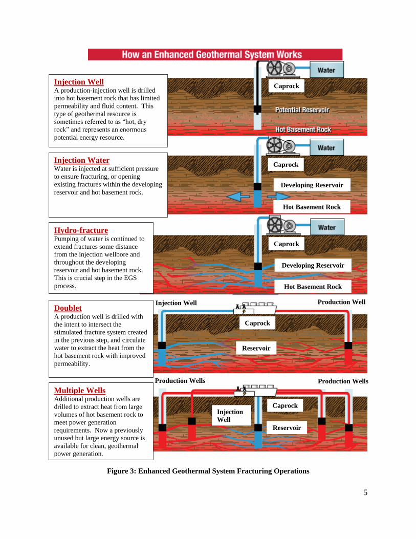
(Environmental Protection Agency, 2004). Fracking operations are shown in Figure 3 (U.S.

Department of Energy, 2012).

5

Figure 3: Enhanced Geothermal System Fracturing Operations

Injection Well A production-injection well is drilled

into hot basement rock that has limited

permeability and fluid content. This

type of geothermal resource is

sometimes referred to as “hot, dry

rock” and represents an enormous

potential energy resource.

Injection Water Water is injected at sufficient pressure

to ensure fracturing, or opening

existing fractures within the developing

reservoir and hot basement rock.

Hydro-fracture Pumping of water is continued to

extend fractures some distance

from the injection wellbore and

throughout the developing

reservoir and hot basement rock.

This is crucial step in the EGS

process.

Injection Well

Production Wells

Multiple Wells Additional production wells are

drilled to extract heat from large

volumes of hot basement rock to

meet power generation

requirements. Now a previously

unused but large energy source is

available for clean, geothermal

power generation.

Doublet A production well is drilled with

the intent to intersect the

stimulated fracture system created

in the previous step, and circulate

water to extract the heat from the

hot basement rock with improved

permeability.

Production Wells

Production Well

Caprock

Injection

Well

Reservoir

Reservoir

Caprock

Caprock

Caprock

Caprock

Developing Reservoir

Hot Basement Rock

Hot Basement Rock

Developing Reservoir

6

2.2.2 Basics of Hydroshearing

Hydroshearing is a relatively new method for producing fractures in impermeable rock.

Hydroshearing occurs when friction is reduced on natural rock fractures by increased water

pressure, which allows the fracture walls to slide past each other. The pressures required for this

process are much less than those needed to break, or frack, the rock. Further, hydroshearing does

not require proppants because the small fractures created will remain slightly open do to the

irregularities on the fracture walls (AltaRock Energy, 2012). Because of natural variations in

rock mass physical properties, structures, and local and regional stress patterns, both fracking

and hydroshearing operations cannot be directionally “controlled” in the same sense that bore-

hole drilling is controlled. In the well bore, stimulation operations may be preceded by explosive

shape charges that pierce the bore-hole casing and cement liner (American Oil and Gas

Historical Society, 2011). These piercing operations can be controlled with reasonable precision

with respect to position and orientation in the hole, but the resulting fractures must be monitored

during the stimulation process to know location and extent.

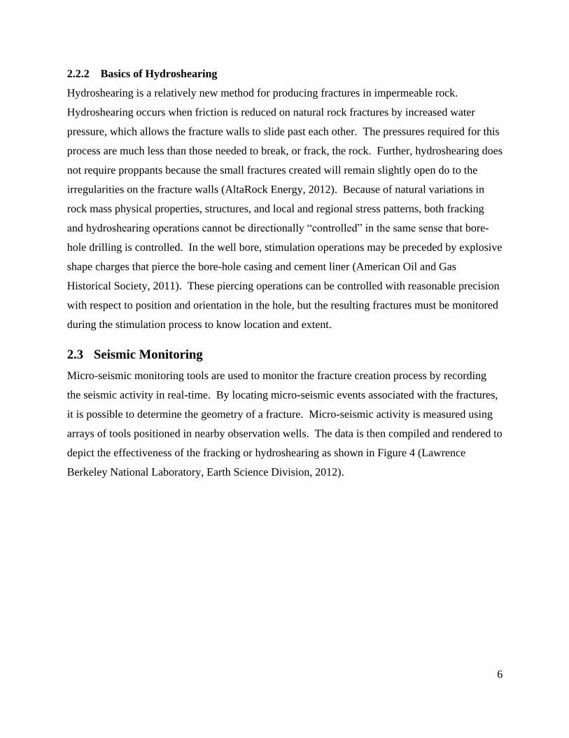
2.3 Seismic Monitoring

Micro-seismic monitoring tools are used to monitor the fracture creation process by recording

the seismic activity in real-time. By locating micro-seismic events associated with the fractures,

it is possible to determine the geometry of a fracture. Micro-seismic activity is measured using

arrays of tools positioned in nearby observation wells. The data is then compiled and rendered to

depict the effectiveness of the fracking or hydroshearing as shown in Figure 4 (Lawrence

Berkeley National Laboratory, Earth Science Division, 2012).

7

Figure 4: Seismic Monitoring Data Plot

Figure 4 is based on the seismic data collected at The Geysers geothermal field in northern

California, the largest single geothermal field in the world. This data is related to the production

and injection phases and used as a general indicator of fluid paths and reservoir response. Each

location where seismic activity occurred was represented by a sphere, color-coded and sized

depending on the magnitude. (Lawrence Berkeley National Laboratory, Earth Science Division,

2012). By closely monitoring this process, the micro-seismic event map reveals the relative size,

location, and orientation of the fracture system. This information can help assess stimulation

effectiveness and provide information necessary to properly create a geothermal reservoir. In

addition, reservoir monitoring of the micro-seismic activity can provide information on reservoir

performance and evolution over time (Henfling, Greving, Maldonado, Chavira, & Uhl, 2010).

8

2.4 Current Technologies

Most micro-seismic monitoring tools used within the oil and gas industry follow the same basic

design. The sensors used to monitor the seismic events must be coupled securely to the bore-

hole wall to ensure reliable data. The coupling force is generally provided by the use of a

coupling arm which extends from the tool securing the device to the bore-hole wall, as shown in

Figure 5 (Mitcham Industires, Inc., 2012).

Figure 5: Sercel Downhole Siesmic Array Systems

The securing of the device is crucial to the tools ability to record accurate seismic data. Because

the same information sought in the oil industry is necessary for enhanced geothermal systems, a

similar tool must be developed with appropriate modifications to survive the environments where

geothermal energy exists.

Chapter 3. REQUIREMENTS, CONSTRAINTS, AND SYSTEM DESIGN

3.1 Environmental Requirements and Constraints

The seismic monitoring tool will be exposed to severe environments that drive the design

parameters of the tool. These same environments preclude application of standard engineering

9

practice for many of the components in the systems that have to be deployed. These

environments are characterized below in terms of chemical or physical attributes.

3.1.1 Physical

The remote environment where the micro-seismic monitoring tool will be used includes high

temperatures, pressures, and corrosive fluids. Depending on the geothermal site, the tool can see

temperatures reaching up to 300 - 400°C (572 - 752°F), (Asmundsson, Normann, Lubotzki, &

Livesay, 2011). This is the primary factor when electronic components are selected. When

constructing a high temperature device, the limiting factor will be the least temperature tolerant

part which limits the selection of components. The tool is often submerged in brine or drilling

mud, which creates a large pressure on the housing of the tool. Depending on the fluid density,

the tool can see pressures up to 1,000 bar (15,000 psi), (Asmundsson, Normann, Lubotzki, &

Livesay, 2011). The tool has to be built to withstand the pressures as well as keep the liquid

from entering sensitive mechanical and electrical components which are completely sealed while

in operation. The tool has to be relatively small and has a unique form factor of being cylindrical

with a large length-to-diameter ratio. This affects the design of the electronics, further limiting

the options for controlling the motor and data collection methods. In addition to these physical

conditions, the tool has to be resistant to attrition that accompanies being handled around well

field operations including shock, bump, and vibration.

3.1.2 Chemical

The tool is submerged in high temperature, electrically conductive and corrosive brines. High

mineral content of the brine means all mechanical components must be designed to prevent or

withstand mineral build-up. The brine is frequently boiling and can have varying ranges of

acidity. Geothermal brines contain a high concentration of dissolved, ionized mineral salts –

mainly chlorides and sulfates, which are highly corrosive. Various corrosive agents and

processes can occur in geothermal brines including the production of hydrogen sulfide, carbon

dioxide, and ammonia (Valdez, Schorr, & Arce, 2006). The hydrogen sulfide can cause

brittleness often referred to as hydrogen embrittlement. Hydrogen embrittlement can damage the

tool housing and the cables used for data communications to the surface (S.P. Lynch, Defence

Science & Technology Organisation, 2007). Based on the brine composition, materials used to

build the tool, and monitoring duration, deposits of arsenic, cyanide, or cadmium can form a

10

scale on the tool. Special care may be required when removing the tool from the bore-hole due

to these toxic substances.

3.2 System Conceptual Design

To survive the environment described, the creation of a monitoring tool that integrated a

mechanical system, which was monitored and controlled by an electrical system, all concurrently

controlled by supporting software was required. The tool is lowered and operated in bore-holes

of various diameters reaching depths of up to 1,500 m (4,921 ft.). The operational depth limit is

primarily dependent upon data transmission lines. At distances greater than 1,500 m (4,921 ft.),

signal distortion can occur when using wire-line (a combination of support cable and electrical

data cables) resulting in faulty data. When the tool is secured at a specified depth in the bore-

hole, data is collected and sent to the surface where it is recorded.

From the system design specifications, the high temperature seismic monitoring tool was adapted

and built with specific requirements to meet design constraints. To secure the seismic sensor to

the bore-hole wall, a mechanical coupling arm is extended by the tool until the desired force is

applied. The monitoring electronics, located within the body of the tool, can monitor and collect

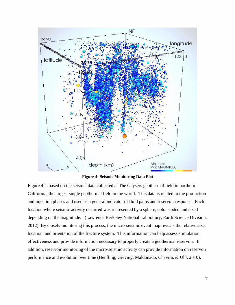
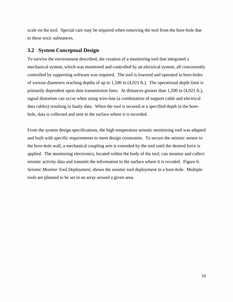
seismic activity data and transmit the information to the surface where it is recoded. Figure 6:

Seismic Monitor Tool Deployment, shows the seismic tool deployment in a bore-hole. Multiple

tools are planned to be set in an array around a given area.

11

Figure 6: Seismic Monitor Tool Deployment

As depicted in Figure 6, the tool is lowered to the pre-determined depth by a logging truck which

uses a winch. Once the tool has reached the appropriate depth, the coupling arm extends,

creating a compressive force between the bore-hole wall and where the seismic signal is sensed.

These vibrations will be recorded by accelerometers within the tool to measure seismic

vibrations. The data is captured and sent to the surface where it is stored. Once the data is

collected, the tool is removed from the bore-hole.

12

Chapter 4. SYSTEM DESIGN SPECIFICATIONS

To meet the requirements and constraints noted in Chapter 3, design specifications were

established.

4.1 Conventional Technology

The prototype seismic tool design was based upon proven technologies utilized by the oil and

gas industry. The tool required modifications to work at the extreme environments including a

new motor and high temperature electronics.

4.2 High Temperature Adaptations

Using design parameters set in Chapter 3, a base-line prototype seismic monitoring system was

designed and built in 2010. Since then, various components have been redesigned and adapted

to further the prototype development. The initial prototype seismic monitoring system was

comprised of three basic elements: 1) a mechanical system that creates the coupling between the

sensors and the bore-hole wall, 2) an electrical system that controls the motor, which controls the

mechanical system, and 3) an operator. During previous applications, deployment of the tool

was controlled by the operator at the surface who would monitor the data and make adjustments.

4.2.1 Mechanical System Specifications

The mechanical system design was modified to work in an operational temperature of 210°C. To

secure the seismic tool to the bore-hole wall, the required force was first characterized. It was

determined that the coupling arm force was proportional to the tool weight, at a minimum rate of

the coefficient of friction between the tool and bore-hole wall. The prototype was built using

stainless steel, weighing close to 27.2 kg (60 lb.) and the basic rule of thumb was to ensure a

radial coupling force between the tool and the bore-hole of five times the tool weight. Based on

the coupling arm force metric, the minimum required extension force was determined to be

approximately 1,334 N (300 lbf.). The required coupling arm force was set at 1,779 N (400 lbf.)

to add a factor of safety to the coupling force and to accommodate the cable weight used to lower

the tool. To provide the driving force to the coupling arm a motor resistant to high temperature

was required and needed to be isolated from the environment. Additionally, the coupling arm

mechanism would be exposed to high pressures and corrosive brines.

13

4.2.2 Electrical System

The electronic system was based upon available technology which is limited in high temperature

environments. A controller was chosen to meet the requirements of the tool based on six

constraints: 1) build size, 2) availability, 3) operational temperature, 4) duration of operational

time at temperature, 5) computational speed, and 6) cost. Build size and availability were

deemed design constraints because of the limited space and time to acquire them. A controller

board that is located down-hole in the tool has to fit within the available space. If the controller

was physically too large or not readily available, it was not chosen to investigate at the

component level. The minimum operational temperature and duration requirements were set at

210°C for 1,000 hours. The data collection system at the tool level was required to have high

computational speed, ensuring the accelerometer data could be reliably collected. Cost was

considered as a comparator driven primarily by the costs of the support materials needed to use

the controller.

4.2.3 Operational System

To deploy the prototype tool, an operator would lower the tool until the required depth was

reached and the coupling arm could be extended. During coupling arm extension, the operator

would monitor the current provided from the power supply until a pre-determined current was

measured which indicated contact with the bore-hole wall. Reliance on the skill, mental

alertness, and responsiveness the operator could yield errors in which the coupling arm’s shear

pin capacity could be exceeded, causing it to break. The tool would then need to be brought back

to the surface for repair before redeployment and this scenario was to be avoided. To limit the

potential for operator error during the extension process, an automated controller system

integrated into the tool is required.

Chapter 5. SEISMIC MONITORING SYSTEM DESIGN MODIFICATIONS

To meet specifications defined in Chapter 4, each of the three basic elements were revaluated: 1)

the mechanical system, 2) the electrical system, and 3) controlling software.

14

5.1 Mechanical System Design

The prototype seismic tool was constructed with stainless steel (type 316 LC) which would allow

the tool to work within the conditions described in Section 3.1. A mechanical power source was

required to supply the force to the coupling arm. Previous hardware limitations resulted in the

use of a stepper motor which produced additional challenges while implementing monitoring

operations. Advances in high temperature components have resulted in the production of DC

motors that meet the temperature requirements for operational use and can be integrated in the

seismic tool. In comparison to a DC motor, a stepper motor requires multiple signals and

additional electronics to run which increase the overall dimensions and weight of the tool. The

benefits of using a DC motor within the tool include: 1) easier to control, 2) can be

simultaneously used with multiple tool systems within the same bore-hole to create a seismic

array, and 3) less controlling circuitry potentially reducing tool size. To further ensure corrosive

brines could not enter and degrade the system, the complete mechanical drive system was

immersed and sealed in an oil reservoir.

5.2 Electrical Design

Three controllers were compared to determine the best option for controlling the seismic tool.

The digital control options compared were the ARM 7 (high temperature version from Texas

Instruments), 8051 (high temperature version from Honeywell), and Field-Programmable Gate

Array (FPGA). During the process for selecting the motor controller, Table 1 was developed to

compare the various technologies, originally produced by Frank Maldonado and Scott Lindblom.

An explanation of the metrics required for the selection matrix is provided in Appendix A.

15

Table 1: Digital Controller Selection Matrix

After comparing the three options, the FPGA was selected to control the system. To reduce

reliance on the operator for the seismic tool’s coupling operations, an integrated solution was

required to measure the force within the existing design. Traditional methods, including the use

of externally placed strain gauges or load cells, were not practical as the harsh conditions would

eventually destroy the sensor. The method used for this application was to measure motor

electrical current, an inexpensive and structurally uncompromising method for determining load.

This could be done because motor power consumption is directly and linearly related to motor

force which creates the coupling force with the bore-hole wall. To measure current, a current

sensing resistor (referred to as a shunt resistor) was required. The voltage drop seen across the

shunt resistor (as a function of current) could be read by the controller and the supporting code

could use this value to control the motor based on the coupling force requirements (Zhen, 2012).

16

5.3 Software Design

To control the FPGA controller required the use of VHDL (a hardware description language used

to describe digital systems). The key advantage of using an FPGA is the ability to conduct

computational processes in parallel versus in series. Operating parallel processes results in a

greater sampling of data over more channels (Chu, 2006). The seismic data collection unit is

operated from the surface, so having the capacity to transmit large volumes of data is necessary.

A flow diagram for developing the software is shown in Figure 7.

Figure 7: FPGA Controller Code Structure

Controlling the coupling arm motor required obtaining analog data from the shunt resistor and

then converting it to a digital signal, where it could be utilized by the program. When the data

was read it was compared to a threshold value (a conditional value which would either run or

stop the motor). If the force was below the desired requirement, the motor would continue to run

until the required force was met as indicated by the voltage across the shunt resistor. This

process ensured proper coupling of the tool to the bore-hole wall. The code followed the logic

flow shown in Figure 8.

file in VHDL

RTL description

synthesis

netlist

placement & routing

configure file

device programming

FPGA chip

delay file

simulation/timing analysis

delay file

simulation

testbench

simulation

17

Figure 8: Current Sensor Code Sequence

In order for the coupling arm to apply the correct force, the threshold values must be determined

based on the bore-hole diameter because the mechanical advantage of the motor output is a

function of arm extension.

Chapter 6. COMPONENT AND SYSTEM TESTING SEQUENCE DESIGN

Testing of the system was conducted in three phases to develop the needed functionality of each

subsystem including the: 1) mechanical system, 2) the electrical system, and 3) the fully

integrated system. Chapter 7 Phase 1: Component Testing describes procedures and results from

the high temperature testing done on the components. Chapter 8 Phase 2: Electro-Mechanical

System Test describes the procedures and results from testing the coupling arm force and current

sensor. This section includes calculations done after the initial characterization tests were

conducted. This initial test measured key outputs to enable selection of a proposed gear box and

electrical current sensor modifications. Based on the initial test, new control values were

integrated into the design and the test sequence was repeated to confirm proper functionality.

Chapter 9 Phase 3: Integrated Software-Electro-Mechanical System Testing describes the testing

of the integrated system with a fully functioning control unit providing feedback between the

coupling arm and motor drive.

ASK FOR CURRENT

SAMPLE READY

OBTAIN SAMPLE

THRESHOLD CONDITION

MOTOR CONTROL

18

Chapter 7. PHASE 1: COMPONENT TESTING

Phase 1 objectives were to verify that both the DC motor and the motor torque sensor worked at

high temperature (up to 210oC for several hours). The motor torque sensor was comprised of an

electrical current sensor because motor torque was found to correlate well with electrical current.

Since the torque sensor design relied on the operational success of the DC motor at high

temperature, the first test conducted was on the motor. If the motor failed, the current sensing

modifications would be conducted based on different motor parameters. Once motor selection

was determined, the electrical current sensor was designed and built. The components used to

create the electrical current sensor were based on proven technology and well characterized

components, so the primary goal was to measure component performance as a function of

temperature. These tests were facilitated with the use of a programmable oven. Upon successful

completion, both components could be integrated to the existing hardware.

7.1 Supporting Equipment

Based on the testing requirements, the equipment used was categorized as being either physical

support equipment or diagnostic equipment. All testing was conducted in a laboratory setting.

7.1.1 Physical Support Equipment

Component characterization at high temperature required the support items listed in Table 2 and

shown in Figure 9.

Figure 9: Component Test Physical Support Equipment

19

Table 2: Component Testing Physical Support Equipment

Item # Item Name Description

1 Fisher Scientific

Isotemp Oven 851F

Oven used to simulate temperatures of operational

environment (vented).

2 Sorensen XHR 60-18 24V DC power supply used to supply power to DC

motor.

3 Agilent E3612A 5V DC power supply used to power current sensor

operational amplifier.

4 KEITHLEY-2400 Current source for current sensor testing.

5 Globe Motor 5A4445 DC motor.

6 One-Piece Rigid

Coupling

Rigid coupling used to connect motor to shaft for

motor testing.

7 1/4in Drive Shaft Extension of Drive Shaft used for motor testing.

8 Unistrut Mounting brackets used to support motor test stand

and mounting motor in oven.

9 Steel motor mount Steel plate machined to house motor for in-oven

testing.

10 Ball Bearing Simulate frictionless surface when load was applied

to drive shaft (preventing drive shaft flex).

11 Pulley (6in radius) Increase lever arm on motor shaft to simulate a

heavier load.

12 Pulley (2in radius) Guide nylon string.

13 32 ounce weight Provides a load on the motor.

14 Rigid ™ Support

Frame

Provide support to complete tool when tested under

load cell.

15 Soldering Iron and

Solder

High temperature soldering iron used to construct

current sensor.

16 Teflon Coated Wire Used in construction of current sensor.

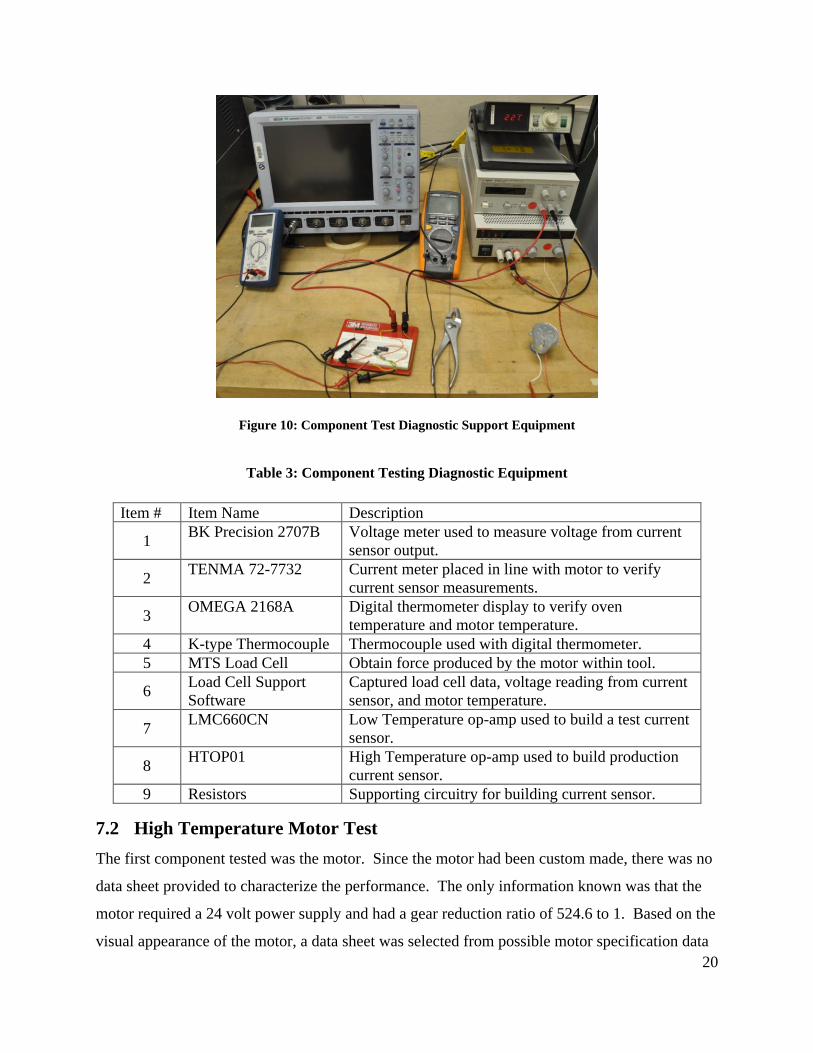
7.1.2 Diagnostic Support Equipment

The equipment used to measure and record data for high temperature component testing is listed

in Table 3 and shown in Figure 10.

20

Figure 10: Component Test Diagnostic Support Equipment

Table 3: Component Testing Diagnostic Equipment


1 BK Precision 2707B Voltage meter used to measure voltage from current

sensor output.

2 TENMA 72-7732 Current meter placed in line with motor to verify

current sensor measurements.

3 OMEGA 2168A Digital thermometer display to verify oven

temperature and motor temperature.

4 K-type Thermocouple Thermocouple used with digital thermometer.

5 MTS Load Cell Obtain force produced by the motor within tool.

6 Load Cell Support

Software

Captured load cell data, voltage reading from current

sensor, and motor temperature.

7 LMC660CN Low Temperature op-amp used to build a test current

sensor.

8 HTOP01 High Temperature op-amp used to build production

current sensor.

9 Resistors Supporting circuitry for building current sensor.

7.2 High Temperature Motor Test

The first component tested was the motor. Since the motor had been custom made, there was no

data sheet provided to characterize the performance. The only information known was that the

motor required a 24 volt power supply and had a gear reduction ratio of 524.6 to 1. Based on the

visual appearance of the motor, a data sheet was selected from possible motor specification data

21

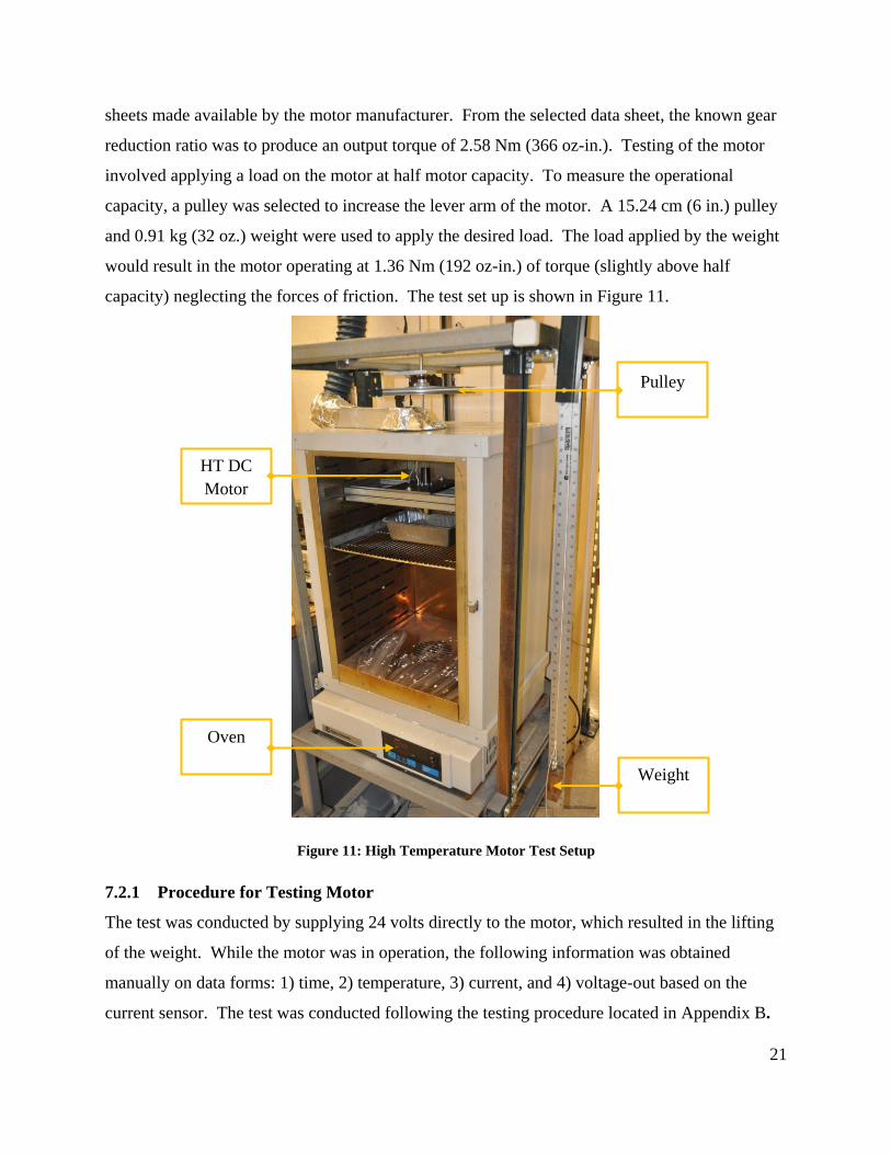
sheets made available by the motor manufacturer. From the selected data sheet, the known gear

reduction ratio was to produce an output torque of 2.58 Nm (366 oz-in.). Testing of the motor

involved applying a load on the motor at half motor capacity. To measure the operational

capacity, a pulley was selected to increase the lever arm of the motor. A 15.24 cm (6 in.) pulley

and 0.91 kg (32 oz.) weight were used to apply the desired load. The load applied by the weight

would result in the motor operating at 1.36 Nm (192 oz-in.) of torque (slightly above half

capacity) neglecting the forces of friction. The test set up is shown in Figure 11.

Figure 11: High Temperature Motor Test Setup

7.2.1 Procedure for Testing Motor

The test was conducted by supplying 24 volts directly to the motor, which resulted in the lifting

of the weight. While the motor was in operation, the following information was obtained

manually on data forms: 1) time, 2) temperature, 3) current, and 4) voltage-out based on the

current sensor. The test was conducted following the testing procedure located in Appendix B.

HT DC

Motor

Oven

Weight

Pulley

22

The voltage-out from the initial trial current sensor was done with a low temperature circuit,

which was placed outside the oven. Figure 12 shows the initial low temperature current sensor

which was supplied 5 volts to amplify the voltage-out signal produced by the shunt resistor

(highlighted in orange).

Figure 12: Initial Trial Current Sensor (Low Temperature)

The description of the resistor selection procedure for the torque sensor is in Appendix C. The

design schematic and support documentation for the low-temperature sensor is in Appendix D.

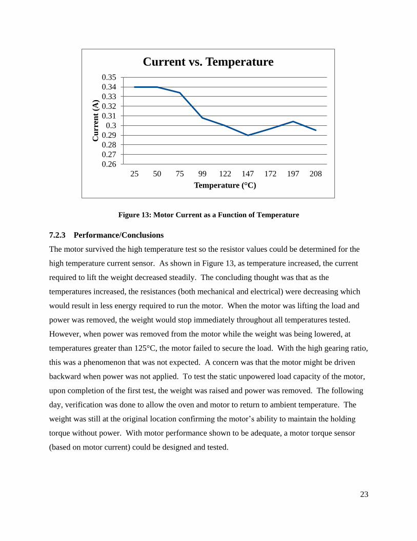
7.2.2 Results

Figure 13 shows the current required by the motor to apply a constant torque when supplied 24

volts at various temperatures.

Shunt

Resistor

23

Figure 13: Motor Current as a Function of Temperature

7.2.3 Performance/Conclusions

The motor survived the high temperature test so the resistor values could be determined for the

high temperature current sensor. As shown in Figure 13, as temperature increased, the current

required to lift the weight decreased steadily. The concluding thought was that as the

temperatures increased, the resistances (both mechanical and electrical) were decreasing which

would result in less energy required to run the motor. When the motor was lifting the load and

power was removed, the weight would stop immediately throughout all temperatures tested.

However, when power was removed from the motor while the weight was being lowered, at

temperatures greater than 125°C, the motor failed to secure the load. With the high gearing ratio,

this was a phenomenon that was not expected. A concern was that the motor might be driven

backward when power was not applied. To test the static unpowered load capacity of the motor,

upon completion of the first test, the weight was raised and power was removed. The following

day, verification was done to allow the oven and motor to return to ambient temperature. The

weight was still at the original location confirming the motor’s ability to maintain the holding

torque without power. With motor performance shown to be adequate, a motor torque sensor

(based on motor current) could be designed and tested.

0.26

0.27

0.28

0.29

0.3

0.31

0.32

0.33

0.34

0.35

25 50 75 99 122 147 172 197 208

Cu

rren

t (A

)

Temperature (°C)

Current vs. Temperature

24

7.3 High Temperature Current Sensor Test

The motor current sensor utilized a single low value resistor, often referred to as a shunt resistor,

to create a voltage-drop that could be measured. Resistor selection required knowing the

maximum current the motor would use. Using the current to directly relate coupling arm force at

the bore-hole wall required the current sensor to operate within a specific range to maximize the

sensitivity of the torque measurement. To obtain the maximum current, the motor was run until

it stalled, resulting in a maximum current of 0.92 A. Using this value, resistors used to amplify

the signal by means of an operational amplifier were selected following the steps described in

Appendix C. Once the values were determined, the sensor was built using high temperature

components and placed in the oven as shown in Figure 14.

Figure 14: High Temperature Current Sensor (Left), Sensor in Oven (Right)

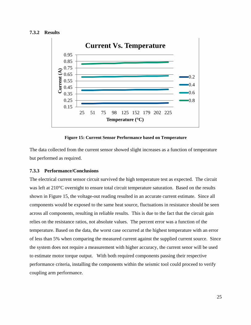
7.3.1 Procedure for Testing Current Sensing

High temperature current sensor testing was conducted in an oven and applying a current from a

current source. When the current sensor was at the temperature desired, current was supplied at

varying amplitudes (0.2, 0.4, 0.6, and 0.8 A) and the output voltage was manually recorded. The

test was conducted following the testing procedure, in Appendix C.

25

7.3.2 Results

Figure 15: Current Sensor Performance based on Temperature

The data collected from the current sensor showed slight increases as a function of temperature

but performed as required.

7.3.3 Performance/Conclusions

The electrical current sensor circuit survived the high temperature test as expected. The circuit

was left at 210°C overnight to ensure total circuit temperature saturation. Based on the results

shown in Figure 15, the voltage-out reading resulted in an accurate current estimate. Since all

components would be exposed to the same heat source, fluctuations in resistance should be seen

across all components, resulting in reliable results. This is due to the fact that the circuit gain

relies on the resistance ratios, not absolute values. The percent error was a function of the

temperature. Based on the data, the worst case occurred at the highest temperature with an error

of less than 5% when comparing the measured current against the supplied current source. Since

the system does not require a measurement with higher accuracy, the current senor will be used

to estimate motor torque output. With both required components passing their respective

performance criteria, installing the components within the seismic tool could proceed to verify

coupling arm performance.

0.15

0.25

0.35

0.45

0.55

0.65

0.75

0.85

0.95

25 51 75 98 125 152 179 202 225

Cu

rren

t (A

)

Temperature (°C)

Current Vs. Temperature

0.2

0.4

0.6

0.8

26

Chapter 8. PHASE 2: ELECTRO-MECHANICAL SYSTEM TEST

Phase 2 objectives were to correlate current as a function of force and verify motor performance

within the tool. The motor would need to generate a force at the bore-hole wall of at least 1,779

N (400 lbf.) at all positions of coupling arm extension. With no information about the level of

torque required to generate the coupling force, preliminary scoping tests were conducted to

correlate motor torque to coupling arm force. In addition to gear reduction, torque produced by

the motor would be amplified by a worm gear of unknown specification located within the tool

housing. Phase 2 testing was conducted in two parts. Initial tests, described in Section 8.1

Initial Electro-Mechanical System Test, were done using parts and design based upon incomplete

knowledge of motor current use, so the data collected did not fully characterize system

performance. Using this preliminary data, calculations described in Section 8.2 Intermediate

Design Calculations Based on Initial Tests, were performed to enable selection of better motor

current sensor resistor and supplemental resistors for magnifying the signal. The final test was

conducted as described in Section 8.3 Final Electro-Mechanical System Test, with components

and equipment that provided an accurate characterization of system performance.

8.1 Initial Electro-Mechanical System Test

To benchmark the electro-mechanical system, a test was conducted to determine the forces that

could be produced at the end of the coupling arm with the use of a hydraulic load cell. The data

acquisition system used to record the load cell data could also monitor the corresponding current

sensor as well as a temperature probe located on the motor.

8.1.1 Support Equipment

Testing required use of the equipment that is listed below and categorized as being either

physical supporting equipment or diagnostic equipment. All testing was conducted in a

laboratory setting.

8.1.1.1 Physical Support Equipment

Physical support equipment used to facilitate the electro-mechanical component testing is listed

in Table 4 and shown in

Figure 16.

27

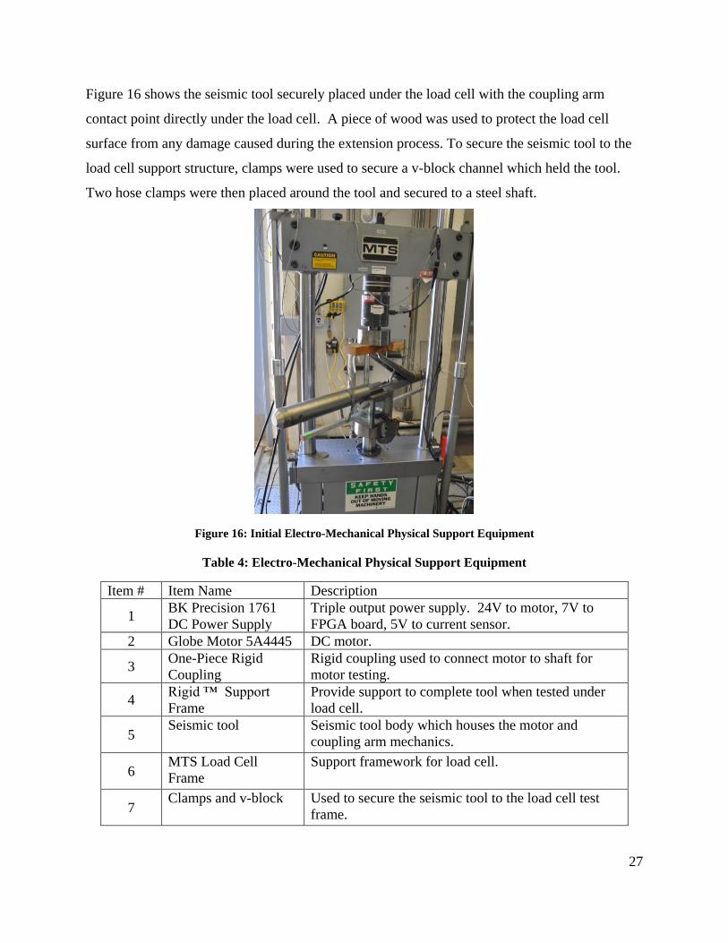
Figure 16 shows the seismic tool securely placed under the load cell with the coupling arm

contact point directly under the load cell. A piece of wood was used to protect the load cell

surface from any damage caused during the extension process. To secure the seismic tool to the

load cell support structure, clamps were used to secure a v-block channel which held the tool.

Two hose clamps were then placed around the tool and secured to a steel shaft.

Figure 16: Initial Electro-Mechanical Physical Support Equipment

Table 4: Electro-Mechanical Physical Support Equipment


1 BK Precision 1761

DC Power Supply

Triple output power supply. 24V to motor, 7V to

FPGA board, 5V to current sensor.


3 One-Piece Rigid

Coupling


motor testing.

4 Rigid ™ Support

Frame


load cell.

5 Seismic tool Seismic tool body which houses the motor and

coupling arm mechanics.

6 MTS Load Cell

Frame

Support framework for load cell.

7 Clamps and v-block Used to secure the seismic tool to the load cell test

frame.

28

8.1.1.2 Diagnostic Support Equipment

Equipment for measuring tool performance data is listed in Table 5 and shown in Figure 17.

Figure 17 shows the testing setup for the initial electro-mechanical testing. The power supply

was replaced from the initial component testing as more supply voltage outputs were required.

Figure 17: Initial Electro-Mechanical Diagnostic Support Equipment

Table 5: Electro-Mechanical Diagnostic Support Equipment



2 MTS Load Cell Obtain force produced by coupling arm.

3 Data Acquisition

System




current sensor.


8.1.2 Procedure for Electro-Mechanical System Test

Before testing could begin, a new mounting bracket was designed to incorporate the motor to the

seismic tool. During the high temperature motor component test, the original coupling adapters

for coupling the motor to the load pulley were deemed unreliable because when applying torque

29

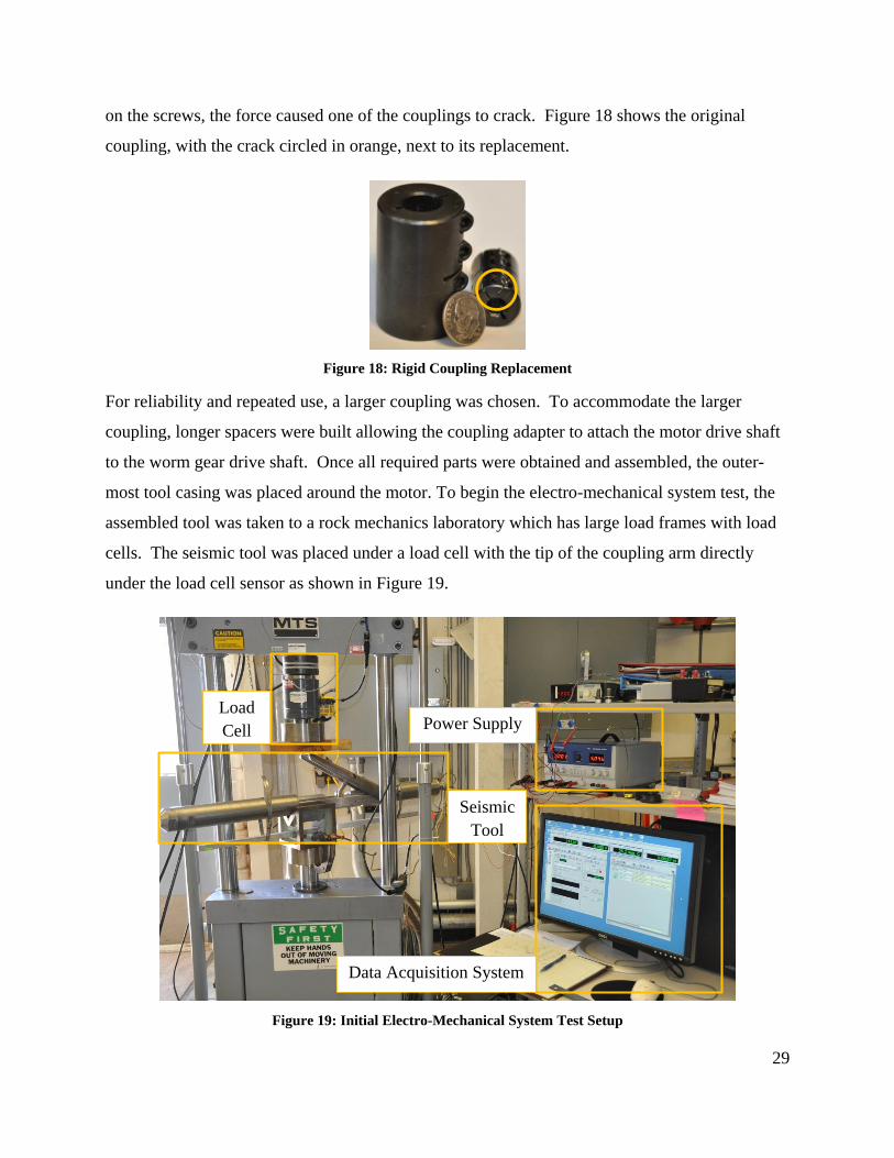
on the screws, the force caused one of the couplings to crack. Figure 18 shows the original

coupling, with the crack circled in orange, next to its replacement.

Figure 18: Rigid Coupling Replacement

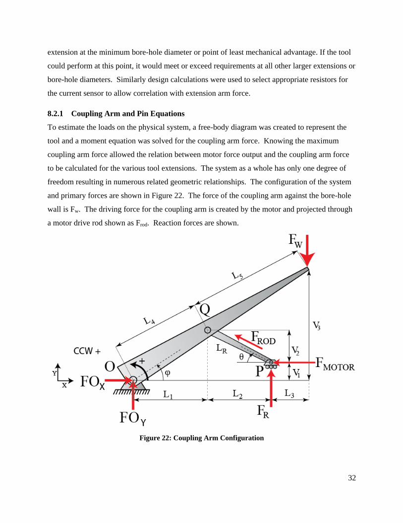
For reliability and repeated use, a larger coupling was chosen. To accommodate the larger

coupling, longer spacers were built allowing the coupling adapter to attach the motor drive shaft

to the worm gear drive shaft. Once all required parts were obtained and assembled, the outer-

most tool casing was placed around the motor. To begin the electro-mechanical system test, the

assembled tool was taken to a rock mechanics laboratory which has large load frames with load

cells. The seismic tool was placed under a load cell with the tip of the coupling arm directly

under the load cell sensor as shown in Figure 19.

Figure 19: Initial Electro-Mechanical System Test Setup

Load

Cell

Seismic

Tool

Power Supply

Data Acquisition System

30

When the motor was supplied 24 volts, the coupling arm would extend up until contact was

achieved. While in motion, the data acquisition system would monitor and record the various

measurements. The recorded data included: 1) time, 2) force applied by coupling arm, 3)

electrical current measurements of the motor, and 4) motor temperature. Tests were conducted at

predetermined coupling arm extensions which were all measured from the tool housing (where

the tool would be in contact with the bore-hole wall) to the endpoint of the arm. Each of these

extensions corresponds to a certain bore-hole diameter constraint. The test operating procedure

is located in Appendix E.

8.1.3 Results

Testing was conducted at coupling arm extensions of 10.16 cm (4 in.), 12.70 cm (5 in.), 15.24

cm (6 in.), 17.78 cm (7 in.), 20.32 cm (8 in.), and 22.86 cm (9 in.) to simulate conditions in bore-

holes of these same diameters. As shown in Figure 20, the motor did not produce the necessary

force on the coupling arm, a limitation of the motor torque. At each extension, the motor was

ran until it stalled.

Figure 20: Coupling Arm Force

10.16 12.70 15.24 17.78 20.32 22.86

Tool Height (in.) 4 5 6 7 8 9

Desired Force (N) 1779.29 1779.29 1779.29 1779.29 1779.29 1779.29

Force Achieved (N) 449.29 519.81 791.71 1056.92 1073.70 1379.19

0

200

400

600

800

1000

1200

1400

1600

1800

2000

Forc

e (N

)

Coupling Arm Extension (cm)

Coupling Arm Force

31

As the force increased on the coupling arm, the current measured stayed at a constant value as

shown in Figure 21. The current sensor values were exceeded at the point of motor stall.

Figure 21: Current Voltage vs. Force at 22.86 cm (9 in.)

8.1.4 Conclusions

At the point of greatest mechanical advantage, the maximum force the seismic tool could

produce was about 1,379 N (310 lbf.), less than the required force level. At positions of less

mechanical advantage, output force was well below the required 1,779 N (400 lbf.) level. Prior

to initial testing, there was no data determining the torque required within the seismic tool to

produce the force needed. Based on the results of this test, supporting calculations were done to

determine what torque the motor would need to produce to generate the required forces.

Initial component testing described in Section 7.3 High Temperature Current Sensor Test, were

unintentionally and unknowingly current limited by the laboratory power supply at 0.92 A. This

test series measured motor current to be as high as 1.5 A when using a different power supply.

Because the electrical current sensor was designed for 0.92 A, subsequent tests would need to be

conducted with a new set of operational amplification resistors to accommodate higher current

levels.

8.2 Intermediate Design Calculations Based on Initial Tests

Because the motor and tool did not perform to the required specifications, the motor gear box

and operational amplification resistors of the tool needed modification. Design calculations were

performed to determine the gear reduction ratio to produce 1,779 N (400 lbf.) at the coupling arm

2.00

2.05

2.10

2.15

2.20C

urr

ent

(A)

Force (N)

Current vs. Force

32

extension at the minimum bore-hole diameter or point of least mechanical advantage. If the tool

could perform at this point, it would meet or exceed requirements at all other larger extensions or

bore-hole diameters. Similarly design calculations were used to select appropriate resistors for

the current sensor to allow correlation with extension arm force.

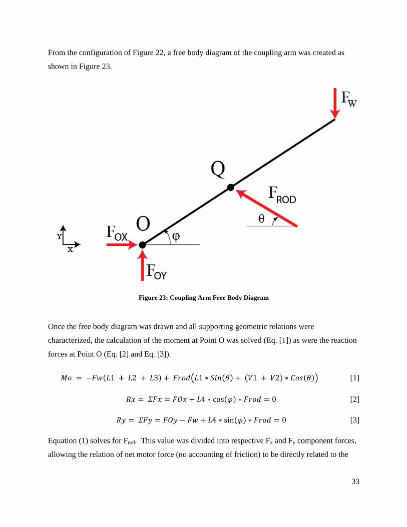
8.2.1 Coupling Arm and Pin Equations

To estimate the loads on the physical system, a free-body diagram was created to represent the

tool and a moment equation was solved for the coupling arm force. Knowing the maximum

coupling arm force allowed the relation between motor force output and the coupling arm force

to be calculated for the various tool extensions. The system as a whole has only one degree of

freedom resulting in numerous related geometric relationships. The configuration of the system

and primary forces are shown in Figure 22. The force of the coupling arm against the bore-hole

wall is Fw. The driving force for the coupling arm is created by the motor and projected through

a motor drive rod shown as Frod. Reaction forces are shown.

Figure 22: Coupling Arm Configuration

33

From the configuration of Figure 22, a free body diagram of the coupling arm was created as

shown in Figure 23.

Figure 23: Coupling Arm Free Body Diagram

Once the free body diagram was drawn and all supporting geometric relations were

characterized, the calculation of the moment at Point O was solved (Eq. [1]) as were the reaction

forces at Point O (Eq. [2] and Eq. [3]).

( ) ( ( ) ( ) ( )) [1]

( ) [2]

( ) [3]

Equation (1) solves for Frod. This value was divided into respective Fx and Fy component forces,

allowing the relation of net motor force (no accounting of friction) to be directly related to the

34

force at the bore-hole wall (Fw). Fx and Fy are the reaction forces on a shear pin located at Point

P, as shown in Figure 24.

Figure 24: Pin Free Body Diagram

( ) [4]

( ) [5]

The shear pin is part of the tool design to allow retraction by force if the motor fails to function,

in which case this pin would shear and free the tool for extraction up the hole. Fx and Fy were

calculated to determine what forces the pin would have to withstand to allow the tool to produce

the force required. The force equations were placed in a spreadsheet where numerous

configurations could be evaluated based on tool geometry. The calculations were based on the

position of the coupling arm, as this could be accurately measured. The forces measured and

shown in Figure 20: Coupling Arm Force were evaluated in the spread sheet and estimates of

frictional forces and maximum motor force were developed. Frictional forces were

characterized as a function of Fw and θ (reference Figure 23). The supporting work for these

calculations is found in Appendix F. Using the estimated frictional forces and the value of

maximum motor force, estimates of forces at the wall were calculated. These are compared in

Figure 25.

35

Figure 25: Coupling Arm Force Calculated vs. Measured

The predicted force values were all trending relatively closely to the measured values but due to

equation simplification, (not including all mechanical losses), the predicted values were slightly

off as shown in Figure 25. Observing the data, the measured force value at 20.32 cm (8in.)

seems to be incorrect which resulted in a larger error of prediction at that extension. At the

lower coupling arm extensions, the majority of the motor force would be applied in an axial

direction while only a fraction of the force would be applied radially out. This resulted in a low

coupling arm force of 449 N (101 lbf.) at the 10.16 cm (4 in) contact point with the bore-hole

wall.

The motor force was inadequate to achieve the needed values of Fw at all extensions, but this

could be addressed by a new motor gear box that would have higher torque and create a higher

axial force.

10.16 12.70 15.24 17.78 20.32 22.86

Tool Height (in.) 4 5 6 7 8 9

Predicted Force (N) 447.88 549.13 736.88 969.17 1266.00 1245.74

Force Achieved (N) 449.29 519.81 791.71 1056.92 1073.70 1379.19

0

200

400

600

800

1000

1200

1400

1600

Forc

e (N

)

Coupling Arm Extension (cm)

Coupling Arm Force

36

8.2.2 Motor Gear Box Calculation

The seismic tool was required to produce an equivalent of 1,779 N (400 lbf.) at the 10.62 cm

(4.18 in.) extension (at the minimum extension level). Based on the relation of torque-to-force at

the 10.62 cm (4.18 in.) bore-hole wall, the required gear ratio could be solved for. Using

interpolation, a relationship was established between the maximum force the tool could produce

at the bore-hole wall, to the torque output of the motor, and subsequently the required gear

reduction ratio. Taking three known values, one unknown was solved for at a time. The steps

taken to solve for the ratios shown in Table 6 are in Appendix G.

Table 6: Gear Box Calculation

Required Motor Torque

RATIO MAX TORQUE

(oz-in.)

MAX TORQUE

(Nm)

MAX Fw

(N)

524.60 366.00 2.58 448.73

639.90 445.00 3.14 545.59

780.60 544.00 3.84 666.97

2077.62 1449.50 10.24 1777.15

To verify gear reduction ratio assumptions were correct, calculated values were compared to

those provided on the motor specifications sheet. Based on the calculations, the motor would

require a gear reduction ratio of about 2078 to 1. The motor manufacturer, Globe Motors, was

contacted to obtain data about their motors and gearbox options. The resulting motor gear box

chosen has a 3,382 to 1 gear reduction ratio with the same motor mount. This replacement motor

meets and exceeds the required motor ratio as shown in orange in Table 6 and could be directly

swapped with the exiting motor.

8.2.3 Electrical Current Sensor Calculation

From the initial electro-mechanical test, the current sensor provided very little useful data

because the current seen by the sensor exceeded the measurable limit. Globe Motors estimated

the maximum ampere rating for the motor to be 1.78 A as shown in Appendix H. A slight

modification to the current sensor was made to reduce the gain so the current seen would result

37

in meaningful data, which followed the same steps in Section 7.3.1 Procedure for Testing

Current Sensing. Additionally, the high temperature operational amplifier had to be replaced

because it had been damaged by an electrical short. This error could have resulted from not

properly grounding the circuit so precautions will be taken to ensure components are grounded.

8.3 Final Electro-Mechanical System Test

Based on the calculations described in Section 8.2.3, new resistors were installed in the

operational amplifier circuit while keeping the original shunt resistor. Since the motor was

unable to produce the required force on the coupling arm, the system was again tested to motor

stall. Comparing the initial to final force values of the electro-mechanical systems test would

ensure repeatability and the new data would yield the appropriate current-to-force relationship.

The rationale for this confirmatory test was based on the premise that the existing motor with a

new gear box could provide adequate power for field applications. The new gearbox would

generate more torque and greater force to the shear pin that drives extension of the coupling arm.

Following the same test procedure from Section 8.1.2 Procedure for Electro-Mechanical System

Test, the new torque sensor (modified with the new op amp) results were found to correlate as

predicted to the coupling arm force.

8.3.1 Results

Testing was conducted at coupling arm extensions of 10.16 cm (4 in.), 12.70 cm (5 in.), 15.24

cm (6 in.), 17.78 cm (7 in.), 20.32 cm (8 in.), and 22.86 cm (9 in.) to simulate conditions in bore-

holes of these same diameters. The data established the relationship between motor electrical

current and coupling arm force as a function of bore-hole diameter. At each extension, the motor

was supplied 24 volts and ran until motor stall resulting in varying forces at the load cell.

Figure 26 shows one example of the force seen by the load cell as a function of time. While

conducting the test, power was supplied until the motor stalled. At the point of stall, power was

removed for approximately three seconds, and then reapplied to help determine the force lost

when the system was allowed relax (absorb mechanical compliance based on construction

tolerances, that is, slack).

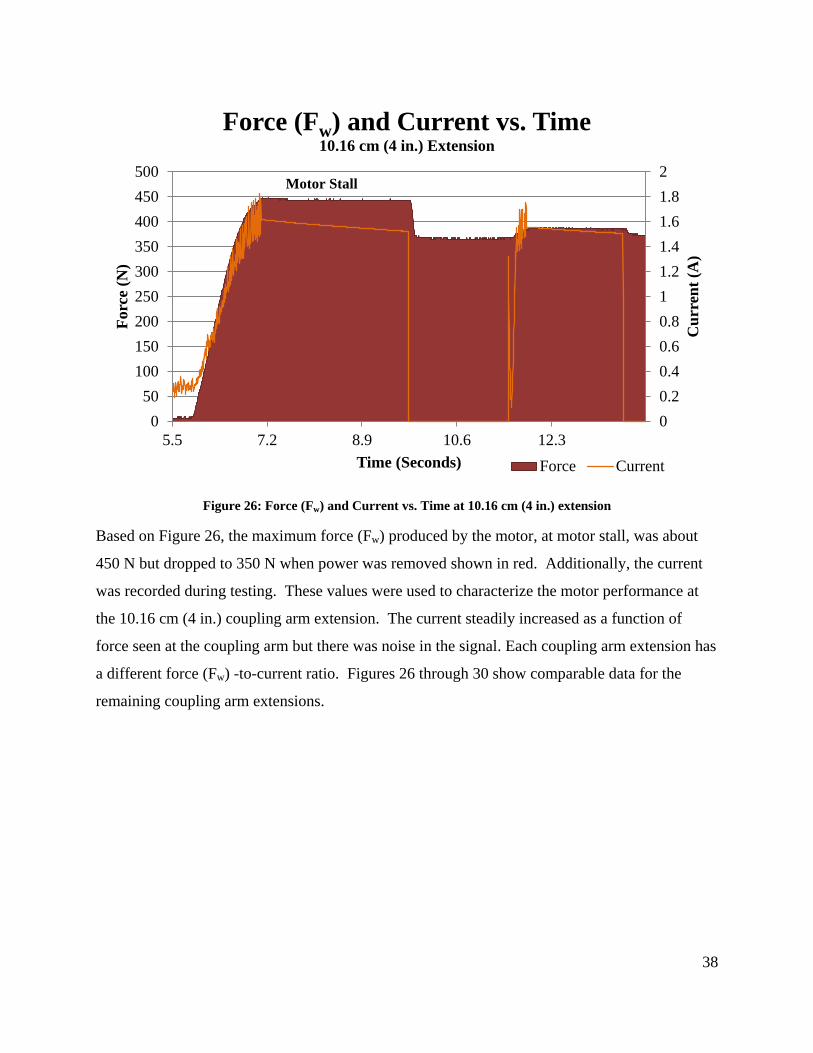
38

Figure 26: Force (Fw) and Current vs. Time at 10.16 cm (4 in.) extension

Based on Figure 26, the maximum force (Fw) produced by the motor, at motor stall, was about

450 N but dropped to 350 N when power was removed shown in red. Additionally, the current

was recorded during testing. These values were used to characterize the motor performance at

the 10.16 cm (4 in.) coupling arm extension. The current steadily increased as a function of

force seen at the coupling arm but there was noise in the signal. Each coupling arm extension has

a different force (Fw) -to-current ratio. Figures 26 through 30 show comparable data for the

remaining coupling arm extensions.

0

0.2

0.4

0.6

0.8

1

1.2

1.4

1.6

1.8

2

0

50

100

150

200

250

300

350

400

450

500

5.5 7.2 8.9 10.6 12.3

Cu

rren

t (A

)

Forc

e (N

)

Time (Seconds)

Force (Fw) and Current vs. Time 10.16 cm (4 in.) Extension

Force Current

Motor Stall

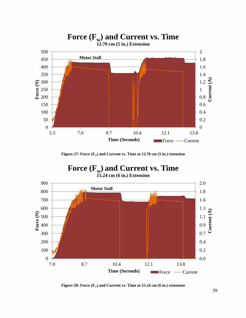
39



0

0.2

0.4

0.6

0.8

1

1.2

1.4

1.6

1.8

2

0

50

100

150

200

250

300

350

400

450

500

5.3 7.0 8.7 10.4 12.1 13.8

Cu

rren

t (A

)

Forc

e (N

)

Time (Seconds)


Force Current

Motor Stall

0.0

0.2

0.4

0.7

0.9

1.1

1.3

1.6

1.8

2.0

0

100

200

300

400

500

600

700

800

900

7.0 8.7 10.4 12.1 13.8

Cu

rren

t (A

)

Forc

e (N

)

Time (Seconds)


Force Current

Motor Stall

40



0.0

0.3

0.7

1.0

1.3

1.7

2.0

0

200

400

600

800

1000

1200

5.7 7.4 9.1 10.8 12.5 14.3

Cu

rren

t (A

)

Forc

e (N

)

Time (Seconds)


Force Current

Motor Stall

0.0

0.3

0.7

1.0

1.3

1.7

2.0

0

200

400

600

800

1000

1200

7.6 9.3 11.0 12.7 14.4 16.2 17.9

Cu

rren

t (A

)

Forc

e (N

)

Time (Seconds)


Force Current

Motor Stall

41


Evaluation of these data show that as the coupling arm extension increased, the amount the

system relaxed decreased which resulted in a greater sustained coupling force at the bore-hole

wall. This was further supported by the calculations done in Section 8.2 Intermediate Design

Calculations Based on Initial Tests where the axial load decreased as coupling arm extension

increased. Furthermore, when current was supplied after the initial coupling of the tool, a large

spike of current was often seen. A software solution will be required to address these

uncontrolled electrical spikes to ensure that the seismic tool is secured with the correct force.

8.4 Electro-Mechanical System Test Summary

The motor torque sensor worked as needed. At each of the different coupling arm extensions,

the current sensor measured values which correlated with the force applied by the coupling arm.

Once these electrical current values were established and categorized based upon bore-hole

diameter, they were input as threshold limits into the controller unit. The values were

specifically picked to ensure a consistent force would result between the coupling arm and bore-

hole wall when the motor is actuated. With the controller programmed, threshold values can be

selected by a seismic test tool operator based upon the supplied bore-hole diameter where the

0.0

0.3

0.5

0.8

1.0

1.3

1.5

1.8

2.0

0

200

400

600

800

1000

1200

1400

1600

5.7 7.5 9.2 10.9 12.6 14.3 16.0

Cu

rren

t (A

)

Forc

e (N

)

Time (Seconds)


Force Current

Motor Stall

42

measurements are being made. With the electro-mechanical system testing completed, the

process of integrating the micro-processor into the rest of the system could begin.

Chapter 9. PHASE 3: INTEGRATED SOFTWARE-ELECTRO-

MECHANICAL SYSTEM TESTING

The Phase 3 testing objective was to produce a closed-loop solution allowing the tool to extend

until the coupling arm reaches the predetermined 1,779 N (400 lbf.) with the bore-hole wall.

Because the motor gear ratio was too high to achieve the required force, the maximum force

achievable was used as the basis for system testing. When the proper gearbox is obtained

electro-mechanical system tests will have to be repeated to obtain the correct current-to-force

relationship values. Using the information provided by Section 8.3 Final Electro-Mechanical

System Test, the controller program was modified to operate the coupling arm.

9.1 Software Controller Testing

Throughout component testing, code was being developed for controlling the system. Using a

reprogrammable FPGA, numerous programming iterations were conducted to achieve the

desired results for tool process control. The FPGA would read in the current sensor data and if

the force was below the desired threshold, the motor would continue to run until the required

force was met as indicated by the voltage across the shunt resistor. The code eventually used

followed the flow diagram shown in Section 5.3, Figure 8: Current Sensor Code Sequence. The

code executes based on a sample rate which was programmed into the FPGA. At the sampling

rate set by the operator, the controller would send a signal to obtain the motor torque which was

the parameter used in the feedback loop to control coupling arm force on the bore-hole wall.

9.1.1 Equipment

The equipment used to conduct these system tests was categorized as either physical supporting

equipment or electrical diagnostic equipment. All testing was conducted in a laboratory setting.

9.1.1.1 Physical Supporting Test Equipment

This testing employed the items listed in Table 7 and the test setup is shown in Figure 32.

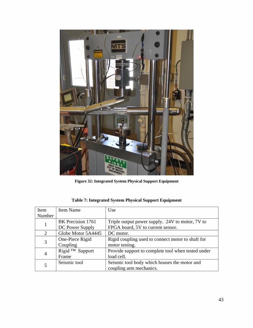
43

Figure 32: Integrated System Physical Support Equipment

Table 7: Integrated System Physical Support Equipment

Item

Number

Item Name Use

1 BK Precision 1761

DC Power Supply

Triple output power supply. 24V to motor, 7V to

FPGA board, 5V to current sensor.


3 One-Piece Rigid

Coupling


motor testing.

4 Rigid ™ Support

Frame


load cell.

5 Seismic tool Seismic tool body which houses the motor and

coupling arm mechanics.

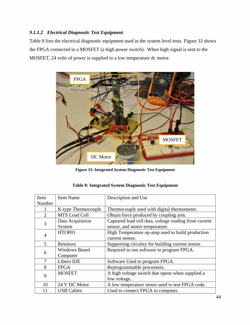
44

9.1.1.2 Electrical Diagnostic Test Equipment

Table 8 lists the electrical diagnostic equipment used in the system level tests. Figure 33 shows

the FPGA connected to a MOSFET (a high power switch). When high signal is sent to the

MOSFET, 24 volts of power is supplied to a low temperature dc motor.

Figure 33: Integrated System Diagnostic Test Equipment

Table 8: Integrated System Diagnostic Test Equipment

Item

Number

Item Name Description and Use


2 MTS Load Cell Obtain force produced by coupling arm.

3 Data Acquisition

System




current sensor.


6 Windows Based

Computer

Required to run software to program FPGA.

7 Libero IDE Software Used to program FPGA.

8 FPGA Reprogrammable processors.

9 MOSFET A high voltage switch that opens when supplied a

low voltage.

10 24 V DC Motor A low temperature motor used to test FPGA code.

11 USB Cables Used to connect FPGA to computer.

FPGA

DC Motor

MOSFET

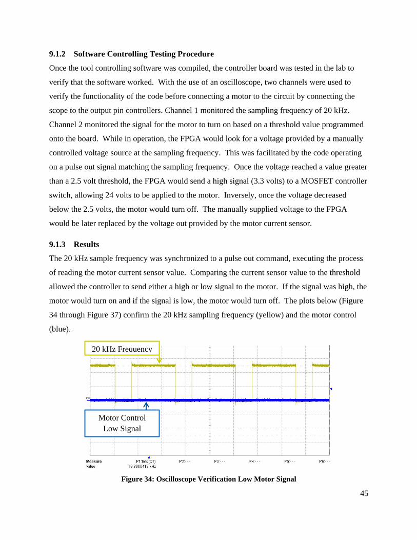
45

9.1.2 Software Controlling Testing Procedure

Once the tool controlling software was compiled, the controller board was tested in the lab to

verify that the software worked. With the use of an oscilloscope, two channels were used to

verify the functionality of the code before connecting a motor to the circuit by connecting the

scope to the output pin controllers. Channel 1 monitored the sampling frequency of 20 kHz.

Channel 2 monitored the signal for the motor to turn on based on a threshold value programmed

onto the board. While in operation, the FPGA would look for a voltage provided by a manually

controlled voltage source at the sampling frequency. This was facilitated by the code operating

on a pulse out signal matching the sampling frequency. Once the voltage reached a value greater

than a 2.5 volt threshold, the FPGA would send a high signal (3.3 volts) to a MOSFET controller

switch, allowing 24 volts to be applied to the motor. Inversely, once the voltage decreased

below the 2.5 volts, the motor would turn off. The manually supplied voltage to the FPGA

would be later replaced by the voltage out provided by the motor current sensor.

9.1.3 Results

The 20 kHz sample frequency was synchronized to a pulse out command, executing the process

of reading the motor current sensor value. Comparing the current sensor value to the threshold

allowed the controller to send either a high or low signal to the motor. If the signal was high, the

motor would turn on and if the signal is low, the motor would turn off. The plots below (Figure

34 through Figure 37) confirm the 20 kHz sampling frequency (yellow) and the motor control

(blue).

Figure 34: Oscilloscope Verification Low Motor Signal

20 kHz Frequency

Motor Control

Low Signal

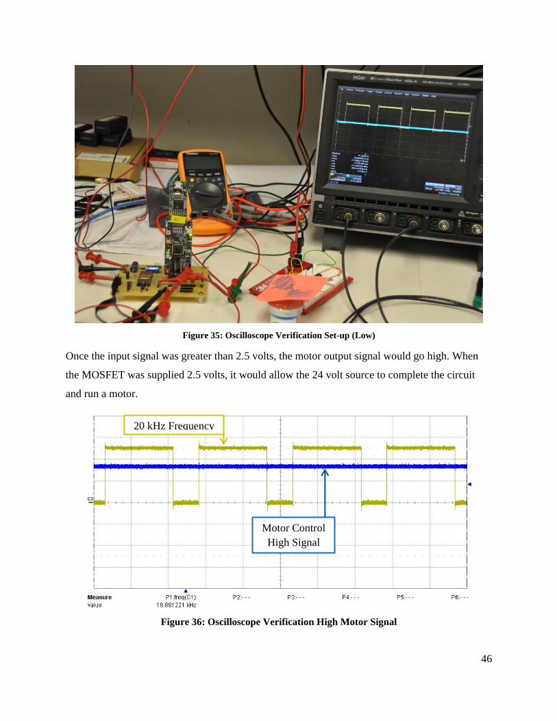
46

Figure 35: Oscilloscope Verification Set-up (Low)

Once the input signal was greater than 2.5 volts, the motor output signal would go high. When

the MOSFET was supplied 2.5 volts, it would allow the 24 volt source to complete the circuit

and run a motor.

Figure 36: Oscilloscope Verification High Motor Signal

20 kHz Frequency

Motor Control

High Signal

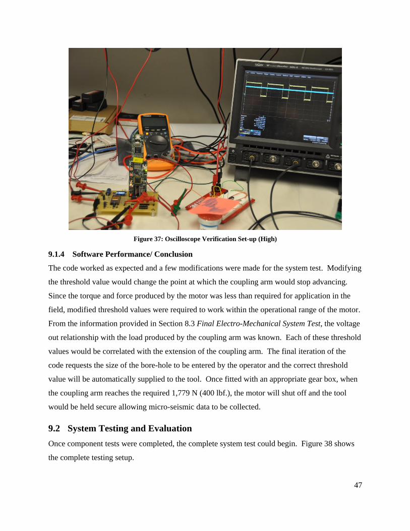
47

Figure 37: Oscilloscope Verification Set-up (High)

9.1.4 Software Performance/ Conclusion

The code worked as expected and a few modifications were made for the system test. Modifying

the threshold value would change the point at which the coupling arm would stop advancing.

Since the torque and force produced by the motor was less than required for application in the

field, modified threshold values were required to work within the operational range of the motor.

From the information provided in Section 8.3 Final Electro-Mechanical System Test, the voltage

out relationship with the load produced by the coupling arm was known. Each of these threshold

values would be correlated with the extension of the coupling arm. The final iteration of the

code requests the size of the bore-hole to be entered by the operator and the correct threshold

value will be automatically supplied to the tool. Once fitted with an appropriate gear box, when

the coupling arm reaches the required 1,779 N (400 lbf.), the motor will shut off and the tool

would be held secure allowing micro-seismic data to be collected.

9.2 System Testing and Evaluation

Once component tests were completed, the complete system test could begin. Figure 38 shows

the complete testing setup.

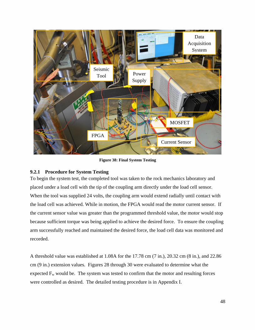
48

Figure 38: Final System Testing

9.2.1 Procedure for System Testing

To begin the system test, the completed tool was taken to the rock mechanics laboratory and

placed under a load cell with the tip of the coupling arm directly under the load cell sensor.

When the tool was supplied 24 volts, the coupling arm would extend radially until contact with

the load cell was achieved. While in motion, the FPGA would read the motor current sensor. If

the current sensor value was greater than the programmed threshold value, the motor would stop

because sufficient torque was being applied to achieve the desired force. To ensure the coupling

arm successfully reached and maintained the desired force, the load cell data was monitored and

recorded.

A threshold value was established at 1.08A for the 17.78 cm (7 in.), 20.32 cm (8 in.), and 22.86

cm (9 in.) extension values. Figures 28 through 30 were evaluated to determine what the

expected Fw would be. The system was tested to confirm that the motor and resulting forces

were controlled as desired. The detailed testing procedure is in Appendix I.

FPGA

Current Sensor

MOSFET

Seismic

Tool

Data

Acquisition

System

Power

Supply

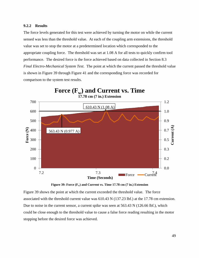
49

9.2.2 Results

The force levels generated for this test were achieved by turning the motor on while the current

sensed was less than the threshold value. At each of the coupling arm extensions, the threshold

value was set to stop the motor at a predetermined location which corresponded to the

appropriate coupling force. The threshold was set at 1.08 A for all tests to quickly confirm tool

performance. The desired force is the force achieved based on data collected in Section 8.3

Final Electro-Mechanical System Test. The point at which the current passed the threshold value

is shown in Figure 39 through Figure 41 and the corresponding force was recorded for

comparison to the system test results.

Figure 39: Force (Fw) and Current vs. Time 17.78 cm (7 in.) Extension

Figure 39 shows the point at which the current exceeded the threshold value. The force

associated with the threshold current value was 610.43 N (137.23 lbf.) at the 17.78 cm extension.

Due to noise in the current sensor, a current spike was seen at 563.43 N (126.66 lbf.), which

could be close enough to the threshold value to cause a false force reading resulting in the motor

stopping before the desired force was achieved.

0.0

0.2

0.3

0.5

0.7

0.9

1.0

1.2

0

100

200

300

400

500

600

700

7.2 7.3 7.4C

urr

ent

(A)

Forc

e (N

)

Time (Seconds)


Force Current

610.43 N (1.08 A)

563.43 N (0.977 A)

50



0.0

0.1

0.3

0.4

0.6

0.7

0.9

1.0

1.2

1.3

0

100

200

300

400

500

600

700

800

900

9.5 9.6 9.7

Cu

rren

t (A

)

Forc

e (N

)

Time (Seconds)


Force Mean Current

710.25 N (1.08 A)

0.0

0.3

0.5

0.8

1.0

1.3

1.5

0

200

400

600

800

1000

1200

5.7 5.8 5.9

Cu

rren

t (A

)

Forc

e (N

)

Time (Seconds)


Force Current

942.77 N (1.08 A)

872.28 N (1.01 A) 912.56 N (1.01 A)

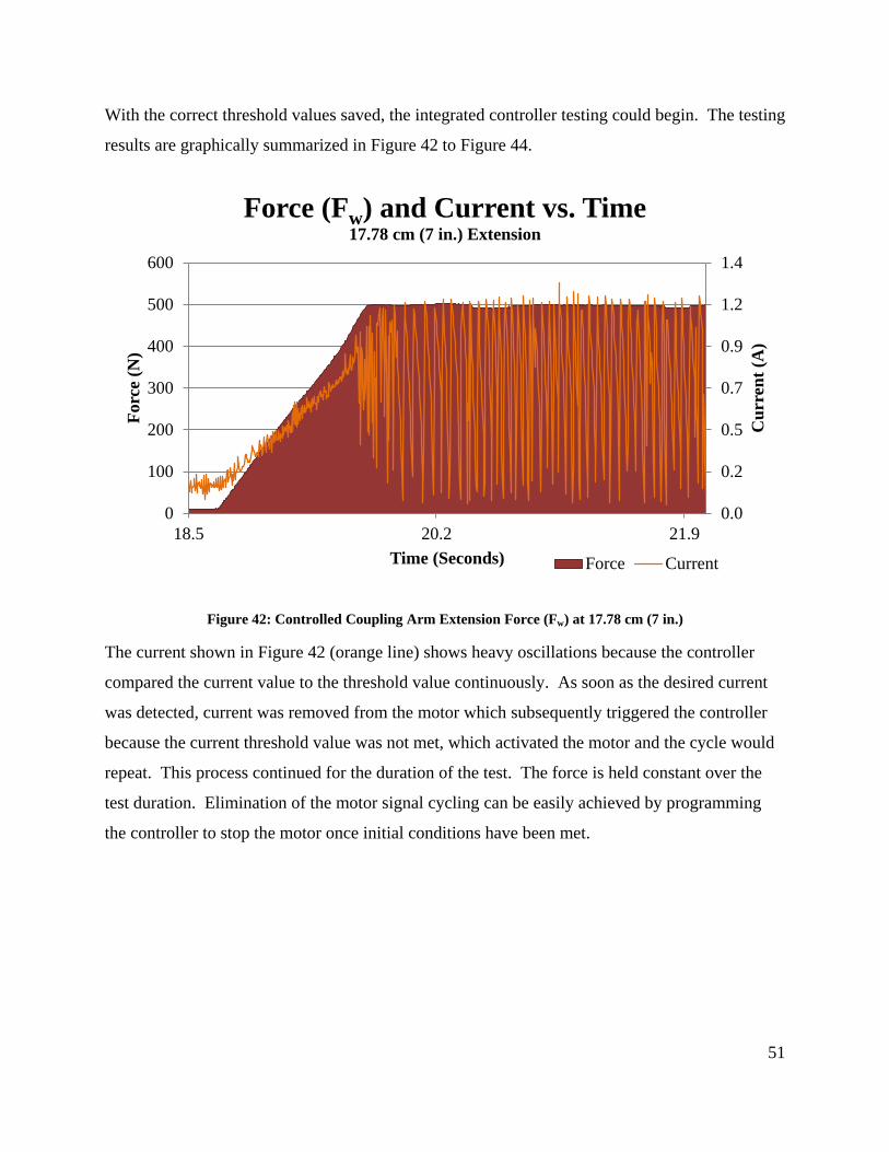
51

With the correct threshold values saved, the integrated controller testing could begin. The testing

results are graphically summarized in Figure 42 to Figure 44.

Figure 42: Controlled Coupling Arm Extension Force (Fw) at 17.78 cm (7 in.)

The current shown in Figure 42 (orange line) shows heavy oscillations because the controller

compared the current value to the threshold value continuously. As soon as the desired current

was detected, current was removed from the motor which subsequently triggered the controller

because the current threshold value was not met, which activated the motor and the cycle would

repeat. This process continued for the duration of the test. The force is held constant over the

test duration. Elimination of the motor signal cycling can be easily achieved by programming

the controller to stop the motor once initial conditions have been met.

0.0

0.2

0.5

0.7

0.9

1.2

1.4

0

100

200

300

400

500

600

18.5 20.2 21.9

Cu

rren

t (A

)

Fo

rce

(N)

Time (Seconds)


Force Current

52

Figure 43: Controlled Coupling Arm Extension Force (Fw) at 20.32 cm (8 in.)

Figure 44: Controlled Coupling Arm Extension Force (Fw) at 22.86 (9 in.)

0.0

0.2

0.4

0.5

0.7

0.9

1.1

1.2

1.4

0

100

200

300

400

500

600

700

800

6.8 8.5 10.2 11.9 13.6 15.3

Cu

rren

t (A

)

Forc

e (N

)

Time (Seconds)


Force Current

0.0

0.2

0.5

0.7

0.9

1.2

1.4

0

200

400

600

800

1000

1200

8.4 10.1 11.8 13.5 15.2

Cu

rren

t (A

)

Forc

e (N

)

Time (Seconds)


Force Current

53

9.3 System Results Summary

Once testing was completed, the desired force values were compared to the obtained controlled

force values shown in Table 9.

Table 9: Current Sensor Performance

Current Sensor Performance

Extension

(cm)

Desired

Force

(N)

Controlled

Force

(N)

Difference

(N)

Extension

(in.)

Desired

Force

(lfb.)

Controlled

Force

(lbf.)

Difference

(lbf.)

%

Error

18.24 610 503 -107 7.18 137 113 -24 -17.54

20.78 710 677 -33 8.18 160 152 -7 -4.65

23.32 942 1043 101 9.18 212 234 23 10.72

Test results confirmed the FPGA code worked but there were errors in accuracy. As the

coupling arm extended, the accuracy was irregular shown in Table 9 (see the % error data). At

the 18.24 cm (7.18 in.) extension, there is a difference of -107 N (24 lbf.) between the desired

force and that applied by the system, a difference of -17.54%. At the operator interface level,

modifications will have to be made to modify the threshold value as needed to meet field

conditions by selecting the bore-hole diameter.

Chapter 10. DISCUSSION AND CONCLUSION

10.1 Discussion

10.1.1 System Performance Observations

System performance results confirmed that when the bore-hole diameter is selected, the coupling

arm extends and could reach the appropriate force, within 100 N (25 lbf.). Three design

modifications could aid in sensor accuracy. First, obtaining an accurate threshold value depends

on the accuracy at which the coupling arm extension can be measured. At each extension, the

force-to-current relationship changes, thus affecting the threshold value. During testing a ruler

was used to measure the distance between the tool housing and the load cell. To increase the

accuracy of this measurement, a sensor should be mounted to the surface of the tool to record the

distance to the load cell platen. The data collected from the distance sensor could then be

54

recorded by the data acquisition system during testing. Second, to increase accuracy of the

sensor, further code modifications need to be made to average the current sensor values because

of the variations seen in Figure 45 to Figure 47. Averaging ten current input values (labeled as

mean current) would result in less noise seen by the FPGA microprocessor. This would

eliminate the possibility of sensing a faulty current reading. A comparison of current sensor data

against mean current sensor data is shown below.

Figure 45: Force (Fw), Current, and Mean Current vs. Time at 17.78 cm (7 in.) Extension

0.00

0.33

0.67

1.00

1.33

1.67

2.00

0

200

400

600

800

1000

1200

6.5 8.2

Cu

rren

t (A

)

Forc

e (N

)

Time (Seconds)

Force (Fw), Current, and Mean Current vs. Time 17.78 cm (7 in.) Extension

Force Current Mean Current

Every 10 Data Points Averaged (Black)

Motor Stall

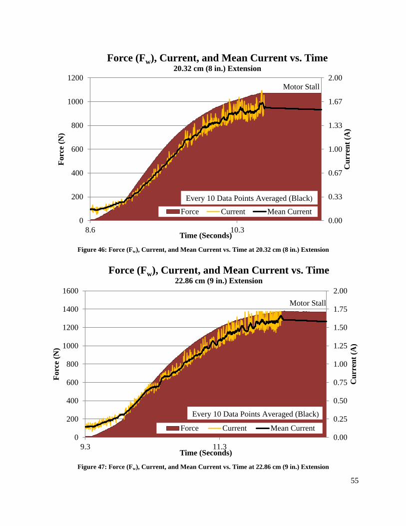
55



0.00

0.33

0.67

1.00

1.33

1.67

2.00

0

200

400

600

800

1000

1200

8.6 10.3

Cu

rren

t (A

)

Forc

e (N

)

Time (Seconds)




Motor Stall

0.00

0.25

0.50

0.75

1.00

1.25

1.50

1.75

2.00

0

200

400

600

800

1000

1200

1400

1600

9.3 11.3

Cu

rren

t (A

)

Forc

e (N

)

Time (Seconds)




Motor Stall

56

Taking the mean of 10 current sensor values reduces the noise seen by the current sensor as

needed. Third, modifying the threshold value, based on laboratory testing to take into account

the error window of the FPGA, could be done. If the current sensor value gets too close to the

threshold position it can prematurely stop motor operations as seen at the 18.24 cm (7.18 in.)

extension in Table 9: Current Sensor Performance. These modifications should be verified to

ensure that appropriate software changes are functioning properly at all extensions.

10.1.2 Mechanical System Sensitivity Analysis

The analyses and data displayed above in Section 8.2 Intermediate Design Calculations Based

on Initial Tests demonstrate that the geometry and configuration of the motor to the coupling arm

extension defines the forces to create the desired contact with the bore-hole wall. This section

evaluates sensitivity to two parameters fundamental to these geometric relations: 1) length of the

motor drive rod and 2) the location where this strut connects to the coupling arm at point Q as

shown in Figure 48.

Figure 48: Configuration of Coupling Arm and Motor Drive Rod

57

Table 10 shows that as the length of the motor drive rod is increased, the bore-hole wall contact

force decreases because the angle θ is low and less force is directed in the radial direction. And

if the rod length was decreased, the opposite effect was seen.

Table 10: Predicted Motor Drive Force as Motor Drive Rod Length Changes

12.70 cm (5 in.) Extension

Motor Drive Rod Length θ Motor Drive Force Fw

cm in. degrees N lbf. N lbf.

7.62 3.00 10.19 18598.16 4186.06 1777.15 400.00

10.16 4.00 7.62 19339.86 4353.00 1777.15 400.00

12.70 5.00 6.09 19471.85 4382.71 1777.15 400.00

15.24 6.00 5.07 19357.32 4356.93 1777.15 400.00

17.78 7.00 4.35 19148.68 4309.97 1777.15 400.00




7.62 3.00 30.74 9747.19 2193.89 1777.15 400.00

10.16 4.00 22.54 10543.18 2373.05 1777.15 400.00

12.70 5.00 17.86 11469.56 2581.56 1777.15 400.00

15.24 6.00 14.81 12173.80 2740.07 1777.15 400.00

17.78 7.00 12.65 12642.48 2845.56 1777.15 400.00




7.62 3.00 67.95 5922.94 1333.13 1777.15 400.00

10.16 4.00 44.04 8095.28 1822.08 1777.15 400.00

12.70 5.00 33.79 7698.89 1732.86 1777.15 400.00

15.24 6.00 27.61 7667.03 1725.69 1777.15 400.00

17.78 7.00 23.41 7866.96 1770.69 1777.15 400.00

Table 11 shows that as the application point of the motor drive rod was moved radially toward

the point of contact with the bore-hole wall, the contact force increased. When the angle

between the coupling arm and the motor drive rod was at 90o, the maximum force was achieved.

Conversely, when the angle between the coupling arm and the motor drive rod was low (when θ

was near zero), contact force decreased because most of the net motor force was directed axially.

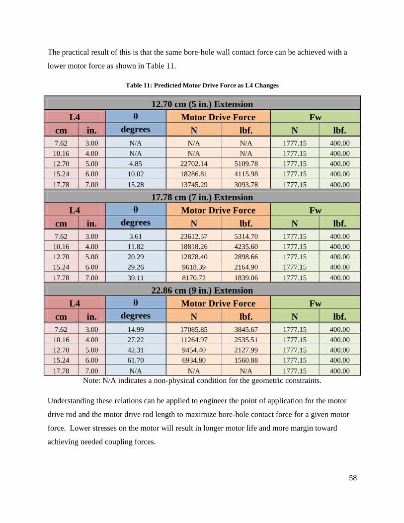
58

The practical result of this is that the same bore-hole wall contact force can be achieved with a

lower motor force as shown in Table 11.

Table 11: Predicted Motor Drive Force as L4 Changes


L4 θ Motor Drive Force Fw


7.62 3.00 N/A N/A N/A 1777.15 400.00

10.16 4.00 N/A N/A N/A 1777.15 400.00

12.70 5.00 4.85 22702.14 5109.78 1777.15 400.00

15.24 6.00 10.02 18286.81 4115.98 1777.15 400.00

17.78 7.00 15.28 13745.29 3093.78 1777.15 400.00




7.62 3.00 3.61 23612.57 5314.70 1777.15 400.00

10.16 4.00 11.82 18818.26 4235.60 1777.15 400.00

12.70 5.00 20.29 12878.40 2898.66 1777.15 400.00

15.24 6.00 29.26 9618.39 2164.90 1777.15 400.00

17.78 7.00 39.11 8170.72 1839.06 1777.15 400.00




7.62 3.00 14.99 17085.85 3845.67 1777.15 400.00

10.16 4.00 27.22 11264.97 2535.51 1777.15 400.00

12.70 5.00 42.31 9454.40 2127.99 1777.15 400.00

15.24 6.00 61.70 6934.80 1560.88 1777.15 400.00

17.78 7.00 N/A N/A N/A 1777.15 400.00

Note: N/A indicates a non-physical condition for the geometric constraints.

Understanding these relations can be applied to engineer the point of application for the motor

drive rod and the motor drive rod length to maximize bore-hole contact force for a given motor

force. Lower stresses on the motor will result in longer motor life and more margin toward

achieving needed coupling forces.

59

10.2 Conclusion

An application to control the coupling force applied to a seismic monitoring tool anchoring

system was created to be deployed down-hole in high-temperature geothermal environments.

This was implemented through a microprocessor and software code that monitored applied force

through a current sensor on a coupling arm drive motor. Once the code was uploaded to the

microprocessor with selected threshold values for the various bore-hole diameters, the system

was put into a closed loop configuration and tested. When powered, the motor was signaled to

turn on and the current sensor values were read verifying a voltage was less than the threshold

value until the desired force was achieved. The tests verified that the motor would stop close to

the correct force loads at the three pre-designated radial extensions.

60

REFERENCES

AltaRock Energy. (2012, March). The Future of Geothermal Energy. Retrieved 4 21, 2012, from

http://blog.newberrygeothermal.com/

American Oil and Gas Historical Society. (2011). Shooters – A “Fracking” History.

http://aoghs.org/technology/shooters-well-fracking-history/. Washington, D. C.:

American Oil and Gas Historical Society.

Asmundsson, R., Normann, R., Lubotzki, H., & Livesay, B. (2011, 24 1). High Temperature

Tools. Retrieved from International Partnership for Geothermal Technology:

http://internationalgeothermal.org/Working_Groups/Documents/Final%20Draft%20Feb

%202012%20-%20High%20Temp%20Tools%20white%20paper.pdf

Chu, P. P. (2006). RTL Hardware Design Using VHDL. Hoboken, New Jersey: John Wiley &

Sons, Inc.

Environmental Protection Agency. (2004, June). Evaluation of Impacts to Underground Sources

of Drinking Water by Hydraulic Fracturing of Coalbed Methane Reservoirs, Final

Report. Washington, D. C.: Environmental Protection Agency.

Henfling, J., Greving, J., Maldonado, F., Chavira, D., & Uhl, J. (2010). Development of a HT

Seismic Monitoring Tool. Innovative Technologies for an Efficient and Reliable

Electricity Supply (CITRES) (pp. 373 - 378 ). IEEE.

Jefferson W. Tester, e. a. (2006). Future of Geothermal Energy. Retrieved 3 19, 2012, from

Idaho National Laboratory:

http://geothermal.inel.gov/publications/future_of_geothermal_energy.pdf

Lawrence Berkeley National Laboratory, Earth Science Division. (2012, 4 21). EGS: Interactive,

Real-Time Map of Earthquakes at The Geysers . Retrieved 4 21, 2012, from Induced

Seismicity: http://esd.lbl.gov/research/projects/induced_seismicity/egs/geysers.html

Majer, E., Baria, R., Stark, M., Smith, B., Oates, S., Bommer, J., & Asanuma, H. (2006, 9 20).

Induced Seismicity. Retrieved 4 19, 2012, from EGS Protocols: http://www.iea-

gia.org/documents/ISWPf1MajerWebsecure20Sep06.doc

Mitcham Industires, Inc. (2012). Mitcham Industries Products. Retrieved 4 22, 2012, from

http://www.mitchamindustries.com/Products/detail.php?pId=107&cat=Sercel

MaxiWave™

61

S.P. Lynch, Defence Science & Technology Organisation. (2007). Progress Towards

Understanding Mechanicsm Of Hydrogen Embrittlement And Stress Corrosion Cracking.

Nashville, Tennessee: NACE International.

U.S. Department of Energy. (2008). An Evaluation of Enhanced Geothermal Systems

Technology. Washington D.C.: U.S. Department of Energy.

U.S. Department of Energy. (2012, 3 30). Geothermal Technologies Program: Energy Basics.

Retrieved 4 21, 2012, from

http://www1.eere.energy.gov/geothermal/geothermal_basics.html

Valdez, B., Schorr, M., & Arce, A. (2006). The Influence of Minerals on Equipment Corrosion in

Geothermal Brines . Retrieved 4 19, 2012, from International Geothermal Association:

http://pangea.stanford.edu/ERE/db/IGAstandard/record_detail.php?id=5514

Williams, C. F., Reed, M. J., Robert, D. H., & Jacob, G. S. (2008, 11 18). USGS. Retrieved 4 16,

2012, from Assessment of Moderate- and High-Temperature Geothermal Resources of

the United States: http://pubs.usgs.gov/fs/2008/3082/

Zhen, Y. (2012, 8 31). Current Sensing Circuit Concepts and Fundamentals. Retrieved 02 24,

2012, from Microchip:

http://www.microchip.com/stellent/idcplg?IdcService=SS_GET_PAGE&nodeId=1824&

appnote=en551198

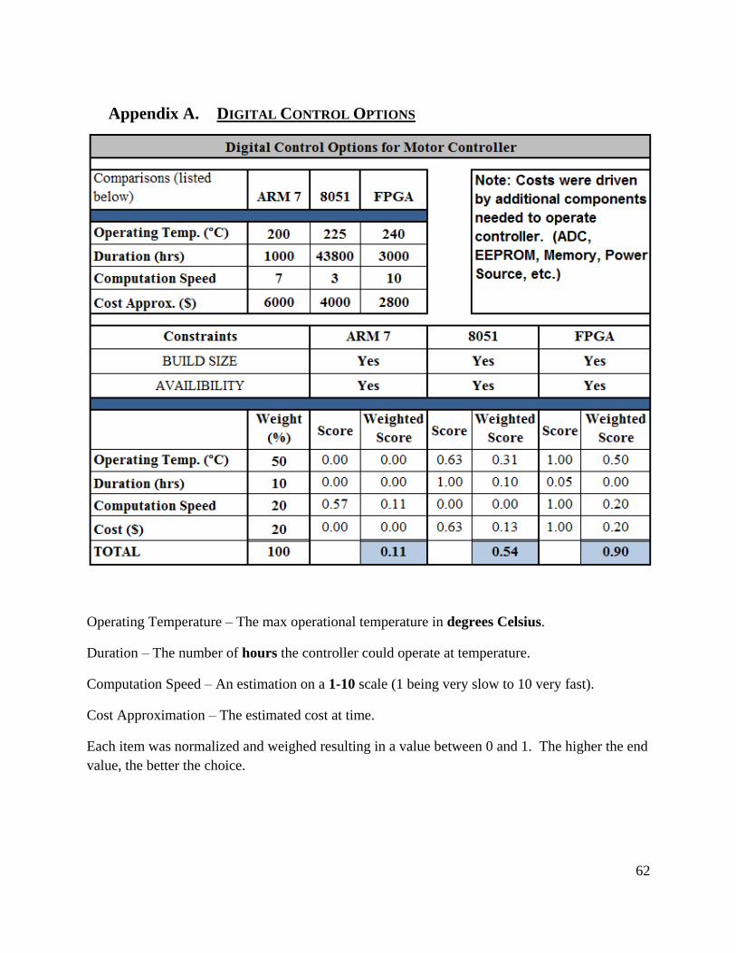
62

Appendix A. DIGITAL CONTROL OPTIONS

Operating Temperature – The max operational temperature in degrees Celsius.

Duration – The number of hours the controller could operate at temperature.

Computation Speed – An estimation on a 1-10 scale (1 being very slow to 10 very fast).

Cost Approximation – The estimated cost at time.

Each item was normalized and weighed resulting in a value between 0 and 1. The higher the end

value, the better the choice.

63

Appendix B. DC MOTOR COMPONENT TEST PROCEDURE

Purpose:

To determine if the DC motor can perform at the desired temperature.

Equipment:

1) Safety Glasses

2) 24V DC power supply (Sorensen XHR 60-18) with wires

3) 5V DC power supply (Agilent E3612A)

4) Voltage Meter (BK Precision 2707B)

5) Current Meter (TENMA 72-7732)

6) Digital Thermometer (OMEGA 2168A with K-type thermocouple)

7) Oven (Fisher Scientific Isotemp Oven Model: 851F)

8) HT DC Motor (Globe Motors: DC Permanent Magnet Gearmotor, A-2030 housing)

9) Motor Couplings

10) Unistrut Housing and Support Structures

11) Pulley with nylon string

Procedure:

Simulated Torque at Temperature:

1) Mount motor securely in oven.

2) Attach motor shaft to ¼ in drive shaft using ½ in coupling with spacers.

3) Attach pulley to ¼ in drive shaft.

4) Secure ¼ in shaft to frame with bearing to reduce chances of bending the drive shaft.

5) Attach 2 lb weight to pulley/string in a manner that it coils evenly.

6) Place thermocouple within oven ensuring cable doesn’t obstruct the drive shaft.

7) Attach a red positive wire connector to DC motor (not plugged into DC power supply).

8) Attach a black negative wire from DC motor to one side of shunt resistor.

9) Attach BK Precision voltmeter to shunt amplified circuit verifying a 5V power supply is

connected to circuit.

10) Attach a negative wire from remaining end of shunt resistor to current meter input.

11) Attach COM from current meter to DC power supply (NEGATIVE).

12) Turn on all power supplies.

64

13) Turn oven on.

14) Set desired temperature.

15) Connect the red positive wire from motor to power supply and record both current and

Vout once the motor has done 1 revolution (ensuring a steady value).

16) Unplug wire from power supply and reverse polarity (swap red and black wires on

motor).

17) Reconnect power supply to return weight to start position.

18) Unplug wire from power supply and reverse polarity.

19) Repeat steps 14 to 18 until motor reaches desired operational temperature of 210°C.

Pass/Fail Criteria: Motor must be operational at 210°C.

65

Appendix C. CURRENT SENSOR DESIGN AND TEST PROCEDURE

Purpose:

To determine the correct resistor values required to amplify the voltage division value based on a 5 volt

power supply. Max Vout will equal 4V.

Equipment:

1) Safety Glasses

2) Honeywell High Temp Op-amp HTOP01

3) Supporting Resistors

4) 0.1 Ω Resistor (Shunt Resistor)

5) High Temperature Solder

6) High Temperature Soldering Iron

7) Teflon Coated Wires

8) 5V DC Power Supply (Agilent 35612A)


10) Oven (Fisher Scientific Isotemp Oven Model: 851F)

11) KEITHLY 2400

Procedure:

1) Find maximum current of motor.

2) Using the following equation to determine gain required:

a. Vout = Gain * (Shunt Resistor Value) * (Max Current)

3) Choose appropriate Resistors.

4) Construct Current Sensor.

5) Suspend Current Sensor in oven.

6) Turn on all power supplies.

7) Turn oven on.

8) Set desired temperature.

9) Connect all required wires.

10) Use KEITHLY to supply required current value when temperature is reached.

11) Repeat steps 8 to 10 until all data is collected.

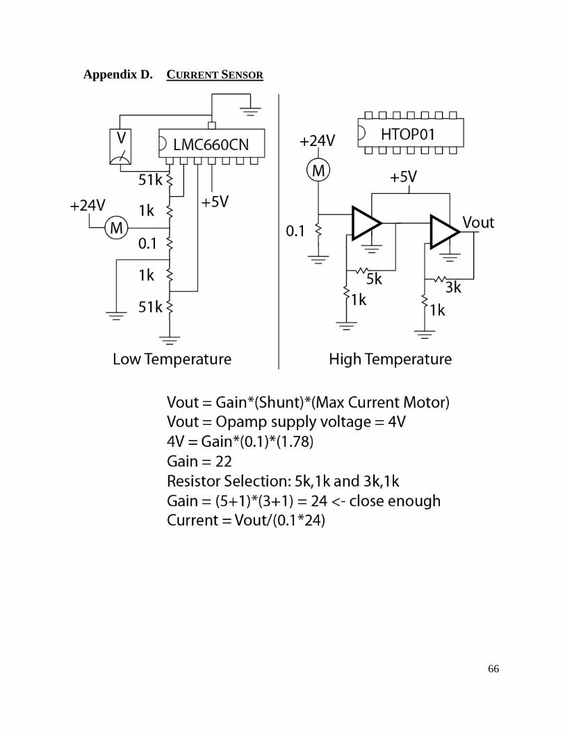
66

Appendix D. CURRENT SENSOR

67

Appendix E. ELECTRO-MECHANICAL SYSTEM TEST

Purpose:

To determine force produced at the end of the coupling arm.

Equipment:

1) Safety Glasses

2) 24V DC power supply (BK Precision 1761) with wires



5) One-Piece Rigid Coupling

6) Rigid ™ Support Frame

7) Seismic tool body

8) MTS Load Cell

9) Data Acquisition System

10) HTOP01

11) Resistors

Procedure:

Simulated Force at Various Bore-Hole Diameters:

1) Place seismic tool under MTS load cell at the point where the coupling arm will make

contact with the center of the sensor.


3) Attach a black negative wire from DC motor to one side of the current sensor.

4) Attach BK Precision voltmeter to current sensor’s amplified circuit verifying a 5V power

supply is connected to circuit.

5) Attach the Vout wire from the current meter to the positive terminal on the DAS.

6) Attach the ground of the DAS to the same ground current sensor is attached to.

7) Connect the thermocouple to the DAS

8) Configure DAS to record data to specified location.

9) Turn on power supplies.

10) Turn hydraulic system on.

11) Set desired coupling arm extension height (on the load cell).

12) Run DAS capture software.

68

13) Connect the red positive wire from motor to power supply and record data from test

(force, temperature, and Vout) until the motor reaches 1779 N (400 lbf.) or stalls.

14) Unplug wire from power supply then reconnect a few times to ensure force is stable.

15) Remove positive wire from power supply.

16) Stop DAS.

17) Remove current sensor from circuit (unplug wire from motor ground).

18) Reverse polarity (swap red and black wires on motor).

19) Reconnect power supply to remove force on load cell.

20) Adjust load cell for next coupling arm extension (ensuring to lock the load cell in place).

21) Unplug wires from power supply, reverse polarity, and connect current sensor.

22) Modify DAS save location for next trial run.

23) Repeat steps 11 to 22 until all coupling arm extension force values are obtained.

24) Remove tool and turn off hydraulic system.

Pass/Fail Criteria: Motor must be capable of producing 1779 N (400 lbf.) at all coupling arm

extensions.

69

Appendix F. COUPLING ARM CALCULATIONS

Procedure for Estimating Frictional Forces:

1 Calculate the net Fx forces of Frod without friction

at all positions.

2 Estimate motor net force with no friction where θ

is near zero (4.14” extension).

3 Estimate frictional forces lost by subtacting the

net Fx from the value in Step 2.

4 Calculate Fy from measured Fw.

5 Divide frictional force by Fy to calculate a

frictional coefficient.

6 Plot frictional coefficient as a function of sine θ

and create a trendline.

7 Using trendline formula, calculate frictional

coefficient at θ = 0.

8 Calculate frictional forces near zero and add this

to the net motor force estimated in Step 2. Set this

equal to maximum motor force.

9 Repeat these steps starting at Step 1 including the

frictional forces calculated in the first iteration.

Make adjustments as appropriate.

With these formulas of friction coefficient and

maximum motor force, net forces on Frod can be

predicted.

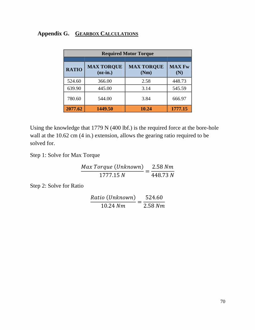
70

Appendix G. GEARBOX CALCULATIONS

Required Motor Torque

RATIO

MAX TORQUE

(oz-in.)

MAX TORQUE

(Nm)

MAX Fw

(N)

524.60 366.00 2.58 448.73

639.90 445.00 3.14 545.59

780.60 544.00 3.84 666.97

2077.62 1449.50 10.24 1777.15

Using the knowledge that 1779 N (400 lbf.) is the required force at the bore-hole

wall at the 10.62 cm (4 in.) extension, allows the gearing ratio required to be

solved for.

Step 1: Solve for Max Torque

( )

Step 2: Solve for Ratio

( )

71

Appendix H. DC MOTOR DATA SHEET

Theoretical stall is 1.79 amps. When power is first applied to the motor, you will see a

momentary current spike and then it drops severely to its running current. The momentary spike

can be as high as the theoretical stall current. For the 5A4445 no load and rated load

performance should fall within the parameters below:

Test Voltage (V) 24

No Load Speed (rpm) 14.1 ~ 17.0

No Load Current (A) 0.20 Max

Normal Rated Load (oz-in) 344

Normal Rated Load

Speed (reference rpm)

10.0 ~ 12.3

Normal Rated Load

Current

(A) .70 Max

72

Appendix I. INTEGRATED SOFTWARE-ELECTRO-MECHANICAL SYSTEM

TEST

Purpose:

To verify the current sensor will stop the coupling arm extension when the required force is

reached.

Equipment:

1) Safety Glasses

2) 24V DC power supply (BK Precision 1761) with wires



5) One-Piece Rigid Coupling

6) Rigid ™ Support Frame

7) Seismic tool body

8) MTS Load Cell

9) Data Acquisition System

10) HTOP01

11) Resistors

Procedure:

Simulated Force at 3 Bore-Hole Diameters (7,8,and 9):

1) Place seismic tool under MTS load cell at the point where the coupling arm will make

contact with the center of the sensor.


3) Attach a black negative wire from DC motor to one side of the current sensor.

4) Attach BK Precision voltmeter to current sensor’s amplified circuit verifying a 5V power

supply is connected to circuit.

5) Attach the Vout wire from the current meter to the positive terminal on the DAS.

6) Attach the ground of the DAS to the same ground current sensor is attached to.

7) Connect the thermocouple to the DAS

8) Configure DAS to record data to specified location.

9) Turn on power supplies.

10) Turn hydraulic system on.

73

11) Set desired coupling arm extension height (on the load cell).

12) Run DAS capture software.

13) Connect the red positive wire from motor to power supply and record data from test

(force, temperature, and Vout) until the motor reaches 1779 N (400 lbf.) or stalls.

14) Unplug wire from power supply then reconnect a few times to ensure force is stable.

15) Remove positive wire from power supply.

16) Stop DAS.

17) Remove current sensor from circuit (unplug wire from motor ground).

18) Reverse polarity (swap red and black wires on motor).

19) Reconnect power supply to remove force on load cell.

20) Adjust load cell for next coupling arm extension (ensuring to lock the load cell in place).

21) Unplug wires from power supply, reverse polarity, and connect current sensor.

22) Modify DAS save location for next trial run.

23) Repeat steps 11 to 22 until all coupling arm extension force values are obtained.

24) Remove tool and turn off hydraulic system.

Pass/Fail Criteria: Extension forces should be limited based on threshold value.