High volatility, thick tails and extreme value theory in ...rgencay/jarticles/ime-thicktails.pdf · R. Gençay et al./Insurance: Mathematics and Economics 33 (2003) 337–356 339

Insurance: Mathematics and Economics 33 (2003) 337–356

High volatility, thick tails and extreme value theoryin value-at-risk estimation

Ramazan Gençaya,∗, Faruk Selçukb,1, Abdurrahman Ulugülyagciba Department of Economics, Carleton University, 1125 Colonel By Drive, Ottawa, Ont., Canada K1S 5B6

b Department of Economics, Bilkent University, Bilkent 06533, Ankara, Turkey

Received 1 August 2002; received in revised form 3 May 2003; accepted 29 July 2003

Abstract

In this paper, the performance of the extreme value theory in value-at-risk calculations is compared to the performances ofother well-known modeling techniques, such as GARCH, variance–covariance (Var–Cov) method and historical simulationin a volatile stock market. The models studied can be classified into two groups. The first group consists of GARCH(1, 1)and GARCH(1, 1)-t models which yield highly volatile quantile forecasts. The other group, consisting of historical simula-tion, Var–Cov approach, adaptive generalized Pareto distribution (GPD) and nonadaptive GPD models, leads to more stablequantile forecasts. The quantile forecasts of GARCH(1, 1) models are excessively volatile relative to the GPD quantile fore-casts. This makes the GPD model be a robust quantile forecasting tool which is practical to implement and regulate for VaRmeasurements.© 2003 Elsevier B.V. All rights reserved.

JEL classification: G0; G1; C1

Keywords: Value-at-risk; Financial risk management; Extreme value theory

1. Introduction

The common lesson from financial disasters isthat billions of dollars can be lost because of poorsupervision and management of financial risks. Thevalue-at-risk (VaR) was developed in response tofinancial disasters of the 1990s and obtained an in-creasingly important role in market risk management.The VaR summarizes the worst loss over a targethorizon with a given level of confidence. It is a pop-ular approach because it provides a single quantity

∗ Corresponding author. Fax:+1-208-693-7012.E-mail addresses: [email protected] (R. Gençay),[email protected] (F. Selçuk).

1 Tel.: +90-312-290-2074; fax:+90-208-694-3196.

that summarizes the overall market risk faced by aninstitution or an individual investor.2

In a VaR context, precise prediction of the probabil-ity of an extreme movement in the value of a portfoliois essential for both risk management and regulatorypurposes. By their very nature, extreme movements arerelated to the tails of the distribution of the underly-ing data generating process. Several tail studies, afterthe pioneering work byMandelbrot (1963a,b), indicatethat most financial time series are fat-tailed.3 Although

2 SeeDowd (1998), Jorion (1997)and Duffie and Pan (1997)for more details on the VaR methodology. For the regulatory rootsof the VaR, seeBasel (1996).

3 See, for example,Dacorogna et al. (2001a,b), Hauksson et al.(2001), Müller et al. (1998), Pictet et al. (1998), Danielssonand de Vries (1997), Ghose and Kroner (1995), Loretan andPhillips (1994), Hols and de Vries (1991), Koedijk et al.

0167-6687/$ – see front matter © 2003 Elsevier B.V. All rights reserved.doi:10.1016/j.insmatheco.2003.07.004

338 R. Gençay et al. / Insurance: Mathematics and Economics 33 (2003) 337–356

these findings necessitate a definition of what is meantby a fat-tailed distribution, there is no unique definitionof fat-tailness (heavy-tailness) of a distribution in theliterature.4 In this study, we consider a distribution tobe fat-tailed if a power decay of the density function isobserved in the tails. Accordingly, an exponential de-cay or a finite endpoint at the tail (the density reachingzero before a finite quantile) is treated as thin-tailed.5

In order to model fat-tailed distributions, the log-normal distribution, generalized error distribution,and mixtures of normal distributions are suggested inmany studies. However, these distributions are thin-tailed according to our definition since the tails ofthese distributions decay exponentially, although theyhave excess kurtosis over the normal distribution. Insome practical applications, these distributions mayfit the empirical distributions up to moderate quan-tiles but their fit deteriorates rapidly at high quantiles(at extremes).

An important issue in modeling the tails is thefiniteness of the variance of the underlying distribu-tion. The finiteness of the variance is related to thethickness of the tails and the evidence of heavy tailsin financial asset returns is plentiful. In his seminalwork, Mandelbrot (1963a,b)advanced the hypothesisof a stable distribution on the basis of an observedinvariance of the return distribution across differentfrequencies and apparent heavy tails in return distri-butions. The issue is that while the normal distribu-tion provides a good approximation to the center ofthe return distribution for monthly (and lower) datafrequencies, there is strong deviation from normalityfor frequencies higher than monthly frequency. Thisimplies that there is a higher probability of extremevalues than for a normal distribution.6 Mandelbrot(1963a,b)provided empirical evidence that the stableLevy distributions are natural candidates for return

(1990), Boothe and Glassman (1987), Levich (1985)and Mussa(1979).

4 SeeEmbrechts et al. (1997, Chapters 2 and 8)for a detaileddiscussion.

5 Although the fourth moment of an empirical distribution (sam-ple kurtosis) is sometimes used to decide on whether an empiricaldistribution is heavy-tailed or not, this measure might be mis-leading. For example, the uniform distribution has excess kurtosisover the normal distribution but it is thin-tailed according to ourdefinition.

6 This indicates that the fourth moment of the return distributionis larger than expected from a normal distribution.

distributions. For excessively fat-tailed random vari-ables whose second moment does not exist, the stan-dard central limit theorem no longer applies, however,the sum of such variables converge to Levy distri-bution within a generalized central limit theorem.Later studies,7 however, demonstrated that the returnbehavior is much more complicated, and follows apower law, which is not compatible with the Levydistribution.

Instead of forcing a single distribution for the entiresample, it is possible to investigate only the tails of thesample distribution using limit laws, if only the tailsare important for practical purposes. Furthermore, theparametric modeling of the tails is convenient for theextrapolation of probability assignments to the quan-tiles even higher than the most extreme observation inthe sample. One such approach is the extreme valuetheory (EVT) which provides a formal framework tostudy the tail behavior of the fat-tailed distributions.

The EVT stemming from statistics has found manyapplications in structural engineering, oceanography,hydrology, pollution studies, meteorology, materialstrength, highway traffic and many others.8 The linkbetween the EVT and risk management is that EVTmethods fit extreme quantiles better than the conven-tional approaches for heavy-tailed data.9 The EVTapproach is also a convenient framework for the sep-arate treatment of the tails of a distribution whichallows for asymmetry. Considering the fact that mostfinancial return series are asymmetric (Levich, 1985;Mussa, 1979), the EVT approach is advantageousover models which assume symmetric distributionssuch ast-distributions, normal distributions, ARCH,GARCH-like distributions except E-GARCH whichallows for asymmetry (Nelson, 1991). Our findingsindicate that the performance of conditional riskmanagement strategies, such as ARCH and GARCH,is relatively poor as compared to unconditional ap-proaches.

The paper is organized as follows. The EVT andVaR estimation are introduced inSections 2 and 3.

7 SeeKoedijk et al. (1990), Mantegna and Stanley (1995), Lux(1996), Müller et al. (1998)and Pictet et al. (1998).

8 For an in-depth coverage of EVT and its applications in financeand insurance, seeEmbrechts et al. (1997), McNeil (1998), Reissand Thomas (1997)and Teugels and Vynckier (1996).

9 SeeEmbrechts et al. (1999)and Embrechts (2000a)for theefficiency of EVT as a risk management tool.

R. Gençay et al. / Insurance: Mathematics and Economics 33 (2003) 337–356 339

Empirical results from a volatile market are presentedin Section 4. We conclude afterwards.

2. Extreme value theory

From the practitioners’ point of view, one of themost interesting questions that tail studies can answeris what are the extreme movements that can be ex-pected in financial markets? Have we already seen thelargest ones or are we going to experience even largermovements? Are there theoretical processes that canmodel the type of fat tails that come out of our empir-ical analysis? Answers to such questions are essentialfor sound risk management of financial exposures. Itturns out that we can answer these questions within theframework of the EVT. Once we know the tail index,we can extend the analysis outside the sample to con-sider possible extreme movements that have not yetbeen observed historically. This can be achieved bycomputation of the quantiles with exceedance proba-bilities.

EVT is a powerful and yet fairly robust frame-work to study the tail behavior of a distribution. Eventhough EVT has previously found large applicabilityin climatology and hydrology, there have also been anumber of extreme value studies in the finance liter-ature in recent years.de Haan et al. (1994)study thequantile estimation using the EVT.Reiss and Thomas(1997) is an early comprehensive collection of sta-tistical analysis of extreme values with applicationsto insurance and finance, among other fields.McNeil(1997, 1998)studies the estimation of the tails ofloss severity distributions and the estimation of thequantile risk measures for financial time series usingEVT. Embrechts et al. (1999)overview the EVT as arisk management tool.Müller et al. (1998)andPictetet al. (1998)study the probability of exceedancesfor the foreign exchange rates and compare themwith the GARCH and HARCH models.Embrechts(1999, 2000a)studies the potentials and limitationsof the EVT. McNeil (1999) provides an extensiveoverview of the EVT for risk managers.McNeiland Frey (2000)study the estimation of tail-relatedrisk measures for heteroskedastic financial time se-ries. Embrechts et al. (1997), Embrechts (2000b)and Reiss and Thomas (1997)are comprehensivesources of the EVT to the finance and insuranceliterature.

3. Value-at-risk

Let rt = log(pt/pt−1) be the returns at timet wherept is the price of an asset (or portfolio) at timet. TheVaRt(α) at the(1 − α) percentile is defined by

Pr(rt ≤ VaRt(α)) = α, (1)

which calculates the probability that returns at timet will be less than (or equal to) VaRt(α), α percentof the time.10 The VaR is the maximum potentialincrease in value of a portfolio given the specifica-tions of normal market conditions, time horizon anda level of statistical confidence. The VaR’s popular-ity originates from the aggregation of several compo-nents of risk at firm and market levels into a singlenumber.

The acceptance and usage of VaR has been spread-ing rapidly since its inception in the early 1990s. TheVaR is supported by the group of 10 banks, the groupof 30, the Bank for International Settlements, and theEuropean Union. The limitations of the VaR are thatit may lead to a wide variety of results under a widevariety of assumptions and methods; focuses on a sin-gle somewhat arbitrary point; explicitly does not ad-dress exposure in extreme market conditions and itis a statistical measure, not a managerial/economicone.11

The methods used for VaR can be grouped underthe parametric and nonparametric approaches. In thispaper, we study the VaR estimation with EVT whichis a parametric approach. The advantage of the EVTis that it focuses on the tails of the sample distribu-tion when only the tails are important for practicalpurposes. Since fitting a single distribution to the en-tire sample imposes too much structure and our needhere is the tails, we adopt the EVT framework whichis what is needed to calculate the VaR. We comparethe VaR calculations with EVT and its performanceto the variance–covariance (Var–Cov) method (para-metric, unconditional volatility), historical simulation(nonparametric, unconditional volatility), GARCH

10 A typical value ofα is 5 or 1%.11 There is a growing consensus among both academicians and

practitioners that the VaR as a measure of risk has serious defi-ciencies. See the special issue of Journal of Banking and Finance26 (7) (2002) on “Statistical and Computational Problems in RiskManagement: VaR and Beyond VaR”.


(1, 1)-t and GARCH(1, 1) with normally distributedinnovations (parametric, conditional volatility).

The Var–Cov method is the simplest approachamong the various models used to estimate the VaR.Let the sample of observations be denoted byrt ,t = 1, 2, . . . , n, wheren is the sample size. Let usassume thatrt follows a martingale process withrt = µt + εt , whereε has a distribution functionFwith zero mean and variance,σ2

t . The VaR in thiscase can be calculated as

VaRt(α) = µt + F−1(α)σt, (2)

whereF−1(α) is the qth quantile(q = 1 − α) valueof the unknown distribution functionF. An esti-mate ofµt andσ2

t can be obtained from the samplemean and the sample variance. Although samplevariance as an estimator of the standard deviationin Var–Cov approach is simple, it has drawbacks athigh quantiles of a fat-tailed empirical distribution.The quantile estimates of the Var–Cov method forthe right tail (left tail) are biased downwards (up-wards) for high quantiles of a fat-tailed empiricaldistribution. Therefore, the risk is underestimatedwith this approach. Another drawback of this methodis that it is not appropriate for asymmetric distri-butions. Despite these drawbacks, this approach iscommonly used for calculating the VaR from holdinga certain portfolio, since the VaR is additive whenit is based on sample variance under the normalityassumption.

Instead of the sample variance, the standard devia-tion in Eq. (2)can be estimated by a statistical model.Since financial time series exhibit volatility cluster-ing, the autoregressive conditional heteroscedasticity(ARCH) (Engle, 1982) and the generalized autore-gressive conditional heteroscedasticity (GARCH)(Bollerslev, 1982) are popular models in practice.Among other studies,Danielsson and Moritomo(2000)andDanielsson and de Vries (2000)show thatthese conditional volatility models with frequent pa-rameter updates produce volatile estimates, and arenot well suited for analyzing large risks. Our findingsprovide further evidence that the performance of con-ditional risk management strategies, such as ARCHand GARCH, is relatively poor as compared to un-conditional approaches. The performance of theseconditional models worsens as one moves further inthe tail of the losses.

4. Empirical findings

A volatile market provides a suitable environmentto study the relative performance of competing VaRmodeling approaches. In this regard, the Turkish econ-omy is a good candidate.12 The Istanbul Stock Ex-change was formally inaugurated at the end of 1985.Following the capital account liberalization in 1989,foreign investors were allowed to purchase and sell alltypes of securities and repatriate the proceeds. The to-tal market value of all traded companies was only US$938 million in 1986 and reached a record level of US$114.3 billion in 1999. Following a major financial cri-sis in February 2001, the total market value of all listedcompanies went down to 33.1 billion by November2001. The daily average trade volume also decreasedfrom the record level US$ 740 million in 2000 to US$336 million in November 2001.Figs. 1 and 2clearlyindicate the high volatility and thick-tail nature of theIstanbul Stock Exchange Index (ISE-100), making ita natural platform to study EVT in financial markets.

4.1. Data analysis

The data set is the daily closings of the IstanbulStock Exchange (ISE-100) Index from 2 November1987 to 8 June 2001. The index value is normalizedto 1 at 1 January 1986 and there are 3383 observa-tions in the data set. The daily returns are defined byrt = log(pt/pt−1), wherept denotes the value of theindex at dayt. In the top panel ofFig. 1the level of theISE-100 Index is presented. The corresponding dailyreturns are displayed in the bottom panel ofFig. 1.The average daily return is 0.22% which implies ap-proximately 77% annual return (260 business days).13

This is not surprising as the economy is a high infla-tion economy. However, 3.27% daily standard devia-tion indicates a highly volatile environment. Indeed,extremely high daily returns (as high as 30.5%) ordaily losses (as low as−20%) are observed during thesample period. Also from a foreign investor’s point ofview, ISE-100 exhibits a wide degree of fluctuationswhich is reflected in its US dollar value. In US dollar

12 For an overview of the Turkish economy in recent years, seeErtugrul and Selçuk (2001). Gençay and Selçuk (2001)studythe recent crises episode in the Turkish economy from the riskmanagement point of view.13 1.0022260 = 1.771.


19.10.89 25.10.91 03.11.93 26.10.95 28.10.97 17.11.990

0.4

0.8

1.2

1.6

2x 10

4

19.10.89 25.10.91 03.11.93 26.10.95 28.10.97 17.11.99

–0.2

–0.1

0

0.1

0.2

0.3

0.4

Fig. 1. Top: daily ISE-100 Index from 2 November 1987 to 8 June 2001 (1 January 1986= 1). The horizontal axis corresponds to timewhile the vertical axis displays the value of the index. The last closing value of the index is 12138.26, implying a daily return of 0.22%(geometric mean) on the average. Bottom: ISE-100 returns calculated byrt = log(pt/pt−1), wherept is the value of the index att. Noticethat there is volatility clustering in the market.


–0.4 –0.3 –0.2 –0.1 0 0.1 0.2 0.30

50

1 00

1 50

2 00

2 50

3 00

0.1 0.15 0.2 0.25 0.30

5

10

15

20

25

Fig. 2. Histogram of daily negative returns (losses) and the best fitted normal distribution,N(µ, σ). Estimated parameters areµ = −0.0022and σ = 0.0327. The right tail region (values overµ + 2σ = 0.0633) is zoomed in the lower panel which indicates a heavy tail.


terms (1986 = 100), the ISE-100 reached a recordlevel of 1654 at the end of the year 1999 and droppeddown to 378 in November 2001.

The sample skewness and kurtosis are 0.18 and8.21, respectively. Although there is no significantskewness, there is excess kurtosis. In the frameworkof this paper, the fat-tailness may not be based on anormality test. Normality tests, such as theBera andJarque (1981)normality test, based on sample skew-ness and sample kurtosis, may not be appropriate sincerejecting normality due to a significant skewness or asignificant excess kurtosis does not necessarily implyfat-tailness. For instance, a distribution may be skewedand thin-tailed or the empirical distribution may haveexcess kurtosis over normal distribution with thin-tails.The first 300 autocorrelations and partial autocorrela-tions of squared returns are statistically significant atseveral lags. This indicates volatility clustering and aGARCH type modeling should be considered in VaRestimations.

Other important tools for the examination of fat-tailness in the data are the sample histogram,QQ (quantile–quantile) plot and the mean excessfunction.14 The sample histogram of negative returns(returns multiplied with−1) is presented inFig. 2.Extreme value analysis works with the right tail ofthe distribution. Hence, we work with negative re-turn distribution where the right tail corresponds tolosses.15 Fig. 2 indicates that extreme realizations aremore likely than a normal distribution would imply.The mean excess plot in the top-left panel ofFig. 3in-dicates a heavy right tail for the loss distribution. QQplot gives some idea about the underlying distributionof a sample. Specifically, the quantiles of an empiricaldistribution are plotted against the quantiles of a hy-pothesized distribution. If the sample comes from thehypothesized distribution or a linear transformationof the hypothesized distribution, the QQ plot shouldbe linear. In extreme value analysis and generalizedPareto models, the unknown shape parameter of thedistribution can be replaced by an estimate as sug-gested byReiss and Thomas (1997, p. 66). If thereis a strong deviation from a straight line, then eitherthe assumed shape parameter is wrong or the model

14 See Reiss and Thomas (1997, Chapters 1 and 2)for someempirical tools for representing data and to check the validity ofthe parametric modeling.15 Hereafter, we will refer to negative returns as losses.

selection is not accurate. In our case, the QQ plot oflosses in the top-right panel ofFig. 3provides furtherevidence for fat-tailness. The losses over a thresholdare plotted with respect to generalized Pareto dis-tribution (GPD) with an assumed shape parameter0.20. The plot clearly shows that the left tail of thedistributions over the threshold value 0.08 is wellapproximated by GPD.

The Hill plot is used to calculate the shape param-eter ξ = 1/α, whereα is the tail index. The shapeparameterξ is informative regarding the limiting dis-tribution of maxima. Ifξ = 0, ξ > 0 or ξ < 0, thisindicates an exponentially decaying, power-decaying,or finite-tail distributions in the limit, respectively.The critical aspect of the Hill estimator is the choiceof the number of upper order statistics. The Hill plotof losses is displayed in the bottom panel ofFig. 3.The stable portion of this figure implies a tail indexestimate between 0.20 and 0.25. Therefore, the Hillestimator indicates a power-decaying tail with an ex-ponent which varies between 4 and 5. This means thatif the probability of observing a return greater thanris p then the probability of observing a loss greaterthankr is in betweenk−4p andk−5p.

4.2. Relative performance

We consider six different models for the one pe-riod ahead loss predictions at different tail quantiles.These models are Var–Cov approach, historical simu-lation, GARCH(1, 1), GARCH(1, 1)-t, adaptive GPDand nonadaptive GPD models.

For the first five models, we adopt a sliding win-dow approach with three different window sizes for500, 1000, and 2000 days.16 For instance, the win-dow is placed between first and 1000th observationsfor a window size of 1000 days and a given quantileis forecasted for the 1001st day. Next, the windowis slided one step forward to forecast quantiles for1002nd, 1003rd,. . . , 3382nd days. The motivationbehind the sliding window technique is to capturedynamic time-varying characteristics of the data indifferent time periods. The last approach (nonadaptiveGPD model) does not utilize a sliding window anduses all the available data up to the day on which fore-casts are generated. This approach is preferable since

16 Danielsson and Moritomo (2000)also adopts a similar win-dowing approach.

344R

.G

ençayet

al./Insurance:M

athematics

andE

conomics

33(2003)

337–356

Fig. 3. Top-left: mean excess (ME) plot. The horizontal axis is for thresholds over which the sample mean of the excesses are calculated. Values on the vertical axis displaythe corresponding mean excesses. The positive trend for thresholds above approximately 0.082 indicates a heavy left tail since this is the mean excess plot for losses. Since anapproximately linear positive trend in an ME plot results from a Pareto type behavior (tail probabilities decaying as a power function), the extreme losses in ISE-100 Index havea Pareto type behavior. Top-right: QQ plot of losses with respect to a GPD (assumed shape parameter,ξ, is 0.20). It shows that the left tail of the distributions over the thresholdvalue 0.08 is well approximated by the GPD. Bottom: variation of the Hill estimate of the shape parameter across the number of upper order statistics. The Hill estimate is verysensitive to the number of upper order statistics. The estimator for the shape parameter should be chosen from a region where the estimate is relatively stable. A stable region istoned gray in the figure. Notice that the confidence bands decrease on the right side of this stability region since more upper order statistics are used to calculate the estimate.


GPD estimation requires more data for out-of-sampleforecasts, as extreme events are rare.17

The GARCH models are parameterized as havingone autoregressive and one moving average term,GARCH(1, 1), since it is practically impossible tofind the best parameterization for each out-of-sampleforecast of a given window size. A similar constraintalso applies for the GPD modeling, i.e., the difficultyof choosing the appropriate threshold value for eachrun. Both the adaptive and nonadaptive GPD quantileforecasts are generated using the upper 2.5% of thesample. In principle, it is possible to choose differentthresholds for different quantiles and different win-dow sizes but this would increase the effect of datasnooping.18 For the historical simulation, piecewiselinear interpolation is chosen to make the empiricaldistribution function one-to-one.19

The relative performance of each model is cal-culated in terms of the violation ratio. A violationoccurs when a realized return is greater than the esti-mated return. The violation ratio is defined as the totalnumber of violations, divided by the total number ofone-period forecasts.20 If the model is correct, the ex-pected violation ratio is the tail area for each quantile.At qth quantile, the model predictions are expected tobe wrong (underpredict the realized return)α = (1−q)

percent of the time. For instance, the model is expectedto underpredict the realized return 5% of the time at the95th quantile. A high violation ratio at each quantileimplies that the model excessively underestimates therealized return (=risk). If the violation ratio at theqthquantile is greater thanα percent, this implies exces-

17 In extreme value analysis, we employed the EVIM toolbox ofGençay et al. (2003).18 SeeSullivan et al. (2001)for the implications of data snooping

in applied studies.19 There are other interpolation techniques such as nonlinear

interpolation or nonparametric interpolation which can also beused.20 For example, for a sample size of 3000, a model with a window

size of 500 days produces 2500 one-step-ahead return estimates fora given quantile. Each of these one-step-ahead returns is comparedto the corresponding realized return. If the realized return is greaterthan the estimated return, a violation occurs. The ratio from totalviolations (total number of times a realized return is greater than thecorresponding estimated return) to the total number of estimates isthe violation ratio. If the number of violations is 125, the violationratio at this particular quantile is 5%(125/2500= 0.05). That is,5% of the time the model underpredicts the return (realized returnis greater than the estimated return).

sive underprediction of the realized return. If the viola-tion ratio is less thanα percent at theqth quantile, thereis excessive overprediction of the realized return by theunderlying model. For example, if the violation ratiois 2% at the 95th quantile, the realized return is only2% of the time greater than what the model predicts.

It is tempting to conclude that a small violation ratiois always preferable at a given quantile. However, thismay not be the case in this framework. Notice that theestimated return determines how much capital shouldbe allocated for a given portfolio assuming that theinvestor has a short position in the market. Therefore,a violation ratio excessively greater than the expectedratio implies that the model signals less capital allo-cation and the portfolio risk is not properly hedged.In other words, the model increases the risk exposureby underpredicting it. On the other hand, a violationratio excessively lower than the expected ratio impliesthat the model signals a capital allocation more thannecessary. In this case, the portfolio holder allocatesmore to liquidity and registers an interest rate loss.A regulatory body may prefer a model overpredictingthe risk since the institutions will allocate more capi-tal for regulatory purposes. Institutions would prefer amodel underpredicting the risk, since they have to al-locate less capital for regulatory purposes, if they areusing the model only to meet the regulatory require-ments. For this reason, the implemented capital allo-cation ratio is increased by the regulatory bodies forthose models that consistently underpredict the risk.

Quantiles which are important for contemporaryrisk management applications as well as regula-tory capital requirements are 0.95th, 0.975th, 0.99th,0.995th and 0.999th quantiles.Table 1 displays theviolation ratios for the left tail (losses) at the windowsize of 1000 observations.21 The numbers in paren-theses are the ranking between six competing modelsfor each quantile. Var–Cov method has the worst per-formance regardless of the window size except for the95th quantile. Since quantiles higher than 0.95th aremore of a concern in risk management applications,we can conclude that the Var–Cov method shouldbe placed at the bottom of the performance rankingof competing models in this particular market. The

21 To minimize the space for tables and the corresponding figureswe report the results for the window size of 1000 observations.The findings for the window sizes of 500 and 2000 observations donot differ from the window size of 1000 observations significantly.


Table 1VaR violation ratios for the left tail (losses) of daily ISE-100 returns (in %)a

5% 2.5% 1% 0.5% 0.1%

Var–Cov 5.37 (2) 3.36 (5) 2.31 (6) 1.60 (5) 0.92 (6)Historical simulation 5.46 (3) 2.73 (2) 1.22 (3) 0.67 (1) 0.34 (4)GARCH(1, 1) 4.70 (1) 2.85 (4) 1.85 (5) 1.34 (4) 0.59 (5)GARCH(1, 1)-t 3.78 (6) 2.23 (3) 1.18 (2) 0.76 (3) 0.21 (2)Adaptive GPD 6.21 (5) 2.73 (2) 1.13 (1) 0.67 (1) 0.25 (3)Nonadaptive GPD 4.41 (4) 2.64 (1) 1.39 (4) 0.71 (2) 0.17 (1)

a The numbers in parentheses are the ranking between six competing models for each quantile. The violation ratio of the best performingmodel is given in italics. Each model is estimated for a rolling window size of 1000 observations. The expected value of the VaR violationratio is the corresponding tail size. For example, the expected VaR violation ratio at 5% tail is 5%. A calculated value greater thanthe expected value indicates an excessive underestimation of the risk while a value less than the expected value indicates an excessiveoverestimation. Daily returns are calculated from the ISE-100 Index. The sample period is 2 November 1987–8 June 2001. The samplesize is 3383 observations. Data source: The Central Bank of the Republic of Turkey.

Table 2VaR violation ratios for the right tail of daily ISE-100 returns (in %)a

5% 2.5% 1% 0.5% 0.1%


a The numbers in parentheses are the ranking between six competing models for each quantile. Each model is estimated for a rollingwindow size of 1000 observations. The expected value of the VaR violation ratio is the corresponding tail size. For example, the expectedVaR violation ratio at 5% tail is 5%. A calculated value greater than the expected value indicates an excessive underestimation of the riskwhile a value less than the expected value indicates an excessive overestimation. Daily returns are calculated from the ISE-100 Index. Thesample period is 2 November 1987–8 June 2001. The sample size is 3383 observations. Data source: The Central Bank of the Republicof Turkey.

second worst model is GARCH(1, 1), except for itsexcellent performance at the 95th quantile. Althoughit performs better than the Var–Cov approach, eventhe simple historical simulation approach producessmaller VaR violation rates than the GARCH modelfor most quantiles.

At the 0.975th quantile, nonadaptive GPD per-forms the best with a violation ratio of 2.64% whichamounts to 0.14% over-rejection. The adaptive GPDmodels follow with 2.73% (0.23% over-rejection)and GARCH-t ranks third with 2.23% (0.27%under-rejection). At the 0.99th quantile, the adaptiveGPD provides the best violation ratio with 1.13%which is followed by GARCH-t with 1.18%. At the0.995th quantile the adaptive GPD and historical sim-ulation provide the best violation ratios with 0.67%which is followed by adaptive GPD with 0.71%. At

the 0.999th quantile, nonadaptive GPD provides thebest performance with 0.17% which is followed byGARCH-t with 0.21%. Overall, the results inTable 1indicate that GPD models provide the best violationratios for quantiles 0.975 and higher. GARCH-t comesclose to being the third contender and competes withthe historical simulation.

Table 2 displays the results for the right tail ofreturns.22 The Var–Cov method is again the worstmodel for the quantiles higher than the 0.95th quan-tile. GARCH(1, 1) performs best at the 0.95th and0.975th quantiles but its performance deteriorates athigher quantiles. GARCH(1, 1)-t provides the best re-sults for quantiles higher than the 0.975th except the

22 It is important to investigate both tails since a financial insti-tution may have a short position in the market.


0.999th quantile where nonadaptive GPD performsbest. Adaptive GPD is the second best for 0.99th and0.995th quantiles. Historical simulation is again an av-erage model.

The one-period ahead 0.99th quantile forecasts ofGARCH(1, 1) and GARCH(1, 1)-t models for lossesare presented inFig. 4 for the window size of 1000.Although the daily quantile forecasts of both modelsare quite volatile, GARCH(1, 1)-t model yields sig-nificantly higher, and therefore more volatile quantileforecasts relative to the GARCH(1, 1) model. Thisimplies that the allocation of the capital for regu-latory purposes has to vary on a daily basis. Thisdaily variation can be as large as 20% which is quitecostly to implement and difficult to supervise inpractice.

24.10.91 02.11.93 25.10.95 27.10.97 16.11.99 –0.2

–0.1

0

0.1

0.2

0.3

0.4

24.10.91 02.11.93 25.10.95 27.10.97 16.11.99 –0.2

–0.1

0

0.1

0.2

0.3

0.4

Fig. 4. Daily ISE-100 Index returns from 2 November 1987 to 8 June 2001. Top: one-period ahead 0.99th quantile forecasts (dotted line)of losses (solid line) using a window size of 1000 with GARCH(1, 1)-t. Bottom: one-period ahead 0.99th quantile forecasts (dotted line)of losses (solid line) using a window size of 1000 with GARCH(1, 1). Note that for volatile periods, GARCH(1, 1)-t gives significantlyhigher quantile estimates.

In the top panel ofFig. 5 quantile forecasts forthe Var–Cov, historical simulation and adaptive GPDmodels are presented. All three models provide ratherstable quantile forecasts across volatile return periods.The Var–Cov and historical simulation quantile fore-casts are always lower than the adaptive GPD fore-casts with Var–Cov quantile forecasts being the mostvolatile between these three models.

A comparison between the GARCH(1, 1)-t andadaptive GPD model is presented in the bottompanel of Fig. 5. This comparison indicates thatGARCH models yield very volatile quantile estimateswhen compared to the GPD, historical simulation orVar–Cov approaches. The volatility of the GARCHquantile forecasts are twice as much of the GPDquantile forecasts in a number of dates. Based on


24.10.91 02.11.93 25.10.95 27.10.97 16.11.99–0.2

–0.15

–0.1

–0.05

0

0.05

0.1

0.15

0.2

LossesVar – CovHSGPD

24.10.91 02.11.93 25.10.95 27.10.97 16.11.99 –0.2

–0.1

0

0.1

0.2

0.3

0.4

LossesGARCH – tGPD

Fig. 5. Daily ISE-100 Index returns from 2 November 1987 to 8 June 2001. Top: one-period ahead 0.99th quantile forecasts of losses usinga window size of 1000 with adaptive GPD, historical simulation and Var–Cov methods. The most conservative quantile forecasts belongto the adaptive GPD model. Bottom: one-period ahead 0.99th quantile forecasts of losses using a window size of 1000 with GARCH(1,1)-t and adaptive GPD methods. It is apparent from the figure that GARCH(1, 1)-t quantile forecasts are much more volatile than theadaptive GPD model. Although the GARCH(1, 1)-t model provides more precise forecasts of this quantile, the excessive volatility of theforecasts of the GARCH(1, 1)-t model should be a concern for a risk manager.

Fig. 5, the level of change in the GARCH quantileforecasts can be as large 20–25% on a daily basis.

It is important that the models to be used in riskmanagement should produce relatively stable quantileforecasts since adjusting the implemented capital fre-quently (daily) in light of the estimated VaR is costly

to implement and regulate. Therefore, models whichyield more stable quantile forecasts may be more ap-propriate for the market risk management purposes. Inthis respect, the GPD models provide robust tail es-timates, and therefore more stable VaR projections inturbulent times.


4.3. S&P-500 returns

Although the Istanbul Stock Exchange Index returnsprovide an excellent environment to study the VaRmodels in high volatility markets with thick-tailed dis-tributions, this data set has not been studied widely inthe literature and is not well known. Hence, we haverepeated the same study with the S&P-500 Index re-turns.

The data set is the daily closings of the S&P-500Index from 3 January 1983 to 31 December 1996 andthere are 3539 observations. The daily returns are de-fined byrt = log(pt/pt−1), wherept denotes the valueof the index at dayt. The top panel ofFig. 6 pro-vides the histogram of the daily S&P-500 daily returnstogether with the best fitted normal distribution. Thelower panel ofFig. 6 provides the zoomed right tailwhich indicates thicker tails. The S&P-500 returns arehighly skewed with a sample skewness of−6.5388and has a large excess kurtosis with a sample kurtosisof 233.79.

The mean excess plot in the top panel ofFig. 7 in-dicates a heavy right tail for the loss distribution. TheQQ plot in the middle panel ofFig. 7provides furtherevidence for fat-tailness. The losses over a thresholdare plotted with respect to the GPD with an assumedshape parameter,ξ = 0.30. It clearly shows that theleft tail of the distributions over the threshold value0.08 is well approximated by GPD. The Hill plot isused to calculate the shape parameterξ = 1/α, whereα is the tail index. The shape parameterξ is infor-mative regarding the limiting distribution of maxima.If ξ = 0, ξ > 0 or ξ < 0, this indicates an expo-nentially decaying, power-decaying, or finite-tail dis-

Table 3VaR violation ratios for the left tail (losses) of daily S&P-500 returns (in %)a

5% 2.5% 1% 0.5% 0.1%


a The numbers in parentheses are the ranking between six competing models for each quantile. Each model is estimated for a rollingwindow size of 1000 observations. The expected value of the VaR violation ratio is the corresponding tail size. For example, the expectedVaR violation ratio at 5% tail is 5%. A calculated value greater than the expected value indicates an excessive underestimation of the riskwhile a value less than the expected value indicates an excessive overestimation. Daily returns are calculated from the S&P-500 Index.The sample period is 3 January 1983–31 December 1996. The sample size is 3539 observations. Data source: Datastream.

tributions in the limit, respectively. The Hill plot oflosses is displayed in the bottom panel ofFig. 7. Thestable portion of this figure implies a tail index esti-mate of 0.40. Therefore, the Hill estimator indicates apower-decaying tail with an exponent of 2.5.

Table 3displays the violation ratios for the left tail(losses) at the window size of 1000 observations. Thenumbers in parentheses are the ranking between sixcompeting models for each quantile. Adaptive GPDmodel provides the best violation ratio for 0.95th and0.975th quantiles. Var–Cov and historical simulationalso do equally well with the adaptive GPD model forthe 0.975th quantile. GARCH-t is the best performerfor the 0.99th quantile which is followed by theadaptive GPD model. The nonadaptive GPD modelprovides the best performance for the 0.995th and0.999th quantiles where the second best performer isthe adaptive GPD model. The results from the left tailanalysis indicate that GPD models provide the best vi-olation ratios in most quantiles. The ranking amongstthe remaining three models is not obvious althoughVar–Cov method receives the worst violation ratios atthe 0.99th quantiles and higher.Table 4displays theresults for the right tail of returns. Amongst five quan-tiles, the adaptive GPD model performs as the bestmodel by ranking first in three quantiles and the sec-ond in the remaining two quantiles. GARCH-t modelhas the worst performance in this tail by ranking asthe last model except at the 0.999th quantile.

The S&P-500 one-period ahead 0.99th quantileforecasts of GARCH(1, 1) and GARCH(1, 1)-t mod-els for negative returns (losses) are presented inFig. 8for the window size of 1000. Although the dailyquantile forecasts of both models are quite volatile,


– 0.2 – 0.1 0 0.1 0.2 0.3 0.40

200

400

600

800

1000

1200

0.05 0.1 0.15 0.2 0.25 0.3 0.35 0.40

5

10

15

20

25

30

Fig. 6. Histogram of S&P-500 daily negative returns (losses) and the best fitted normal distribution,N(µ, σ). Estimated parameters areµ = −0.0003 andσ = 0.0115. The right tail region (values overµ + 2σ = 0.0227) is zoomed in the lower panel. The sample period is 3January 1983 to 31 December 1996. The sample size is 3539 observations.


0 0.01 0.02 0.03 0.04 0.05 0.06 0.07 0.08 0.09 0.10

0.01

0.02

0.03

0.04

0.05

0.06

0.07

0.08

0.09

0.1

Threshold

Mea

n E

xces

s

0.01 0.02 0.03 0.04 0.05 0.06 0.07 0.08 0.090.01

0.02

0.03

0.04

0.05

0.06

0.07

0.08

0.09

GP

D Q

uant

iles

Ordered Data

0 20 40 60 80 100 120 140 160 180 200

– 0.2

0

0.2

0.4

0.6

0.8

1

1.2

1.4

1.6

Order Statistics

xi

Fig. 7. Top: ME plot; middle: QQ plot; bottom: Hill plot of the S&P-500 returns. The sample period is 3 January 1983 to 31 December1996. The sample size is 3539 observations.


Table 4VaR violation ratios for the right tail of daily S&P-500 returns (in %)a

5% 2.5% 1% 0.5% 0.1%


a The numbers in parentheses are the ranking between six competing models for each quantile. Each model is estimated for a rollingwindow size of 1000 observations. The expected value of the VaR violation ratio is the corresponding tail size. For example, the expectedVaR violation ratio at 5% tail is 5%. A calculated value greater than the expected value indicates an excessive underestimation of the riskwhile a value less than the expected value indicates an excessive overestimation. Daily returns are calculated from the S&P-500 Index.The sample period is 3 January 1983–31 December 1996. The sample size is 3539 observations. Data source: Datastream.

12.12.86 05.12.98 27.11.90 17.11.92 09.11.94 31.10.96–0.05

0

0.05

0.1

0.15

12.12.86 05.12.98 27.11.90 17.11.92 09.11.94 31.10.96–0.05

0

0.05

0.1

0.15

Fig. 8. Top: S&P-500 one-period ahead 0.99th quantile forecasts (dotted line) of losses (solid line) using a window size of 1000 withGARCH(1, 1)-t. Bottom: one-period ahead 0.99th quantile forecasts (dotted line) of losses (solid line) using a window size of 1000 withGARCH(1, 1). Note that for volatile periods GARCH(1, 1)-t gives significantly higher quantile estimates. We restricted the vertical axisto [−0.05, 0.15] to improve the resolution. Otherwise GARCH quantile forecasts are as large as 0.34.


GARCH(1, 1)-t model yields significantly higher, andtherefore more volatile quantile forecasts relative tothe GARCH(1, 1) model. This implies that the alloca-tion of the capital for regulatory purposes has to varyon a daily basis. This daily variation can be as large as

12.12.86 05.12.98 27.11.90 17.11.92 09.11.94 31.10.96– 0.05

0

0.05

0.1

0.15LossesVar – CovHSGPD

12.12.86 05.12.98 27.11.90 17.11.92 09.11.94 31.10.96– 0.05

0

0.05

0.1

0.15LossesGARCH – tGPD

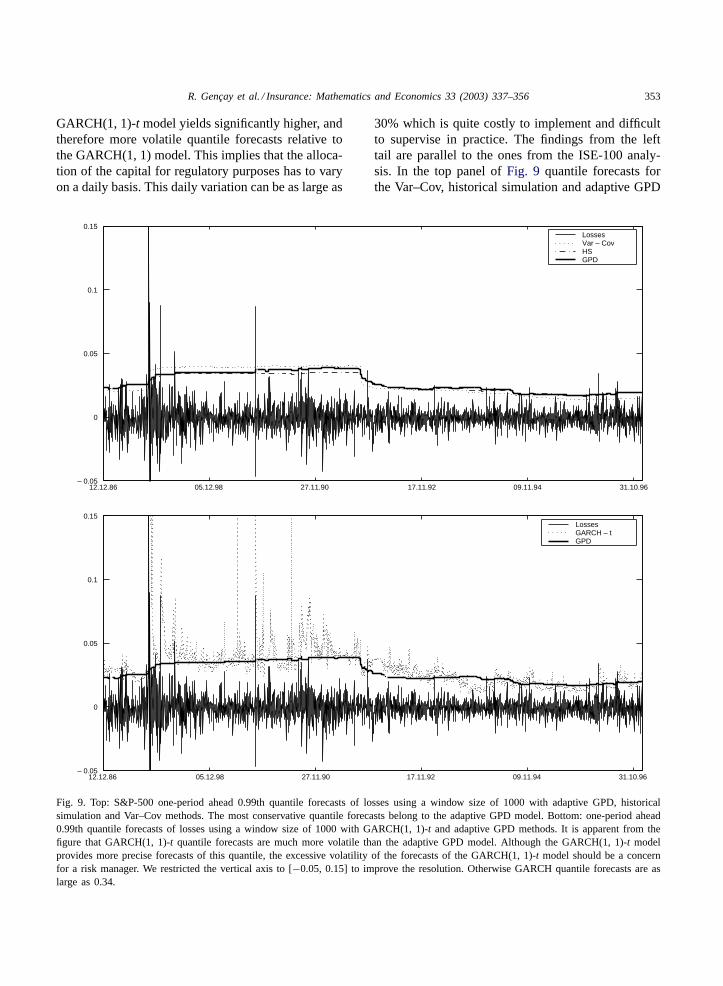
Fig. 9. Top: S&P-500 one-period ahead 0.99th quantile forecasts of losses using a window size of 1000 with adaptive GPD, historicalsimulation and Var–Cov methods. The most conservative quantile forecasts belong to the adaptive GPD model. Bottom: one-period ahead0.99th quantile forecasts of losses using a window size of 1000 with GARCH(1, 1)-t and adaptive GPD methods. It is apparent from thefigure that GARCH(1, 1)-t quantile forecasts are much more volatile than the adaptive GPD model. Although the GARCH(1, 1)-t modelprovides more precise forecasts of this quantile, the excessive volatility of the forecasts of the GARCH(1, 1)-t model should be a concernfor a risk manager. We restricted the vertical axis to [−0.05, 0.15] to improve the resolution. Otherwise GARCH quantile forecasts are aslarge as 0.34.

30% which is quite costly to implement and difficultto supervise in practice. The findings from the lefttail are parallel to the ones from the ISE-100 analy-sis. In the top panel ofFig. 9 quantile forecasts forthe Var–Cov, historical simulation and adaptive GPD


models are presented. All three models provide ratherstable quantile forecasts across volatile return periods.The Var–Cov and historical simulation quantile fore-casts follow similar time paths as the adaptive GPDquantile forecasts.

A comparison between the GARCH(1, 1)-t andadaptive GPD model is presented in the bottompanel of Fig. 9. This comparison indicates thatGARCH models yield very volatile quantile estimateswhen compared to the GPD, historical simulation orVar–Cov approaches. The volatility of the GARCHquantile forecasts are multiples of the GPD quantileforecasts in a number of dates. Based onFig. 9, thelevel of change in the GARCH quantile forecasts canbe as large as 30% on a daily basis. Our findings fromthe S&P-500 returns confirm the findings obtainedfrom the ISE-100 returns that the GPD model pro-vides more accurate violation ratios and its quantileforecasts are stable across turbulent times.

From a regulatory point of view, it is importantthat banks maintain enough capital to protect them-selves against extreme market conditions. This con-cern allows regulators to impose minimum capitalrequirements in different countries. In 1996, the BaselCommittee recommended a framework for measur-ing market risk and credit risk, and for determiningthe corresponding capital requirements, seeBasel(1996).23 The committee proposes two different waysof calculating the minimum capital risk requirement:a standardized approach and an internal risk man-agement model. In the standardized approach, banksare required to slot their exposures into differentsupervisory categories. These categories have fixedrisk weights set by the regulatory authorities. A bankcan utilize its own internal risk management model,subject to approval by the authorities. These modelsmust meet certain conditions. Our “violation ratio”above as a criterion for evaluation of different modelsis basically the Basel Committee criterion for evalu-ating internal risk management models. We showedthat this criterion, in combination with volatile mar-

23 The New Basel Capital Accord (Basel II) is expected to befinalized by the end of 2003 with implementation to take placein member countries by year-end 2006. According to a recentconsultative document by Basel Committee, the new accord sub-stantially changes the treatment of credit risk and introduces anexplicit treatment operational risk; seehttp://www.bis.orgfor fur-ther details.

ket conditions, may result in costly implementations,especially if conditional models are employed tomeasure the risk. The results also indicate that theexisting Basel Committee risk measurement and reg-ulatory framework can be improved by incorporatingcosts of trading, costs of capital adjustments andthe amount of losses into the existing criterion todetermine minimum capital requirements.

5. Conclusions

Risk management gained importance in the lastdecade due to the increase in the volatility of financialmarkets and a desire of a less fragile financial sys-tem. In risk management, the VaR methodology as ameasure of market risk is popular with both financialinstitutions and regulators. VaR methodology benefitsfrom the quality of quantile forecasts. In this study,conventional models such as GARCH, historical sim-ulation and Var–Cov approaches, are compared toEVT models. The six models used in this study canbe classified into two groups: one group consisting ofGARCH(1, 1) and GARCH(1, 1)-t models which leadto highly volatile quantile forecasts, while the othergroup consisting of historical simulation, Var–Cov,adaptive GPD and nonadaptive GPD models providemore stable quantile forecasts. In the first group,GARCH(1, 1)-t, while in the second group the GPDmodel is preferable for most quantiles.

Our results suggest further study by constructinga cost function that penalizes the excessive volatilityand rewards the accuracy of the quantile forecasts atthe same time. The results also indicate that the exist-ing Basel committee risk measurement and regulatoryframework can be improved by incorporating costs oftrading, costs of capital adjustments and the amountof losses into existing criterion to determine minimumcapital requirements.

Acknowledgements

Ramazan Gençay gratefully acknowledges financialsupport from the Swiss National Science Foundationunder NCCR–FINRISK, Natural Sciences and Engi-neering Research Council of Canada and the SocialSciences and Humanities Research Council of Canada.

http://www.bis.org


References

Basel, 1996. Overview of the Amendment to the Capital Accordto Incorporate Market Risk. Basel Committee on BankingSupervision, Basel.

Bera, A., Jarque, C., 1981. Efficient tests for normality, hetero-scedasticity and serial independence of regression residuals:Monte Carlo evidence. Economics Letter 7, 313–318.

Bollerslev, T., 1982. Generalized autoregressive conditionalheteroscedasticity. Journal of Econometrics 31, 307–327.

Boothe, P., Glassman, P.D., 1987. The statistical distribution ofexchange rates. Journal of International Economics 22, 297–319.

Dacorogna, M.M., Pictet, O.V., Müller, U.A., de Vries, C.G.,2001a. Extremal forex returns in extremely large datasets.Extremes 4, 105–127.

Dacorogna, M.M., Gençay, R., Müller, U.A., Olsen, R.B., Pictet,O.V., 2001b. An Introduction to High-frequency Finance.Academic Press, San Diego, CA.

Danielsson, J., de Vries, C.G., 1997. Tail index and quantileestimation with very high frequency data. Journal of EmpiricalFinance 4, 241–257.

Danielsson, J., de Vries, C.G., 2000. Value-at-risk and extremereturns. Annales D’Economie et de Statistique 60, 239–270.

Danielsson, J., Moritomo, J., 2000. Forecasting extreme financialrisk: a critical analysis of practical methods for the Japanesemarket. Monetary Economic Studies 12, 25–48.

de Haan, L., Jansen, D.W., Koedijk, K.G., de Vries, C.G.,1994. Safety first portfolio selection, extreme value theory andlong run asset risks. In: Galambos, J., Lechner, J., Kluwer,E.S. (Eds.), Extreme Value Theory and Applications. KluwerAcademic Publishers, Dordrecht, pp. 471–488.

Dowd, K., 1998. Beyond Value-at-Risk: The New Science of RiskManagement. Wiley, Chichester, UK.

Duffie, D., Pan, J., 1997. An overview of value-at-risk. Journal ofDerivatives 7, 7–49.

Embrechts, P., 1999. Extreme value theory in finance andinsurance. Department of Mathematics, ETH, Swiss FederalTechnical University.

Embrechts, P., 2000a. Extreme value theory: potentials andlimitations as an integrated risk management tool. DerivativesUse, Trading and Regulation 6, 449–456.

Embrechts, P., 2000b. Extremes and Integrated Risk Management.Risk Books and UBS Warburg, London.

Embrechts, P., Kluppelberg, C., Mikosch, C., 1997. ModelingExtremal Events for Insurance and Finance. Springer, Berlin.

Embrechts, P., Resnick, S., Samorodnitsky, G., 1999. Extremevalue theory as a risk management tool. North AmericanActuarial Journal 3, 30–41.

Engle, R.F., 1982. Autoregressive conditional heteroscedasticmodels with estimates of the variance of United Kingdominflation. Econometrica 50, 987–1007.

Ertugrul, A., Selçuk, F., 2001. A brief account of the Turkisheconomy: 1980–2000. Russian East European Finance Trade37, 6–28.

Gençay, R., Selçuk, F., 2001. Overnight borrowing, interest ratesand extreme value theory. Department of Economics, BilkentUniversity.

Gençay, R., Selçuk, F., Ulugülyagcı, A., 2003. EVIM: a softwarepackage for extreme value analysis in Matlab. Studies inNonlinear Dynamics and Econometrics 5, 213–239.

Ghose, D., Kroner, K.F., 1995. The relationship between GARCHand symmetric stable distributions: finding the source of fattails in the financial data. Journal of Empirical Finance 2, 225–251.

Hauksson, H.A., Dacorogna, M., Domenig, T., Müller, U.,Samorodnitsky, G., 2001. Multivariate extremes, aggregationand risk estimation. Quantitative Finance 1, 79–95.

Hols, M.C., de Vries, C.G., 1991. The limiting distribution ofextremal exchange rate returns. Journal of Applied Econo-metrics 6, 287–302.

Jorion, P., 1997. Value-at-Risk: The New Benchmark forControlling Market Risk. McGraw-Hill, Chicago.

Koedijk, K.G., Schafgans, M.M.A., de Vries, C.G., 1990. Thetail index of exchange rate returns. Journal of InternationalEconomics 29, 93–108.

Levich, R.M., 1985. Empirical studies of exchange rates: pricebehavior, rate determination and market efficiency. Handbookof Economics 6, 287–302.

Loretan, M., Phillips, P.C.B., 1994. Testing the covariancestationary of heavy-tailed time series. Journal of EmpiricalFinance 1, 211–248.

Lux, T., 1996. The stable Paretian hypothesis and the frequency oflarge returns: an examination of major German stocks. AppliedFinancial Economics 6, 463–475.

Mandelbrot, B., 1963a. New methods in statistical economics.Journal of Political Economy 71, 421–440.

Mandelbrot, B., 1963b. The variation of certain speculative prices.Journal of Business 36, 394–419.

Mantegna, R.N., Stanley, H.E., 1995. Scaling behavior in thedynamics of an economic index. Nature 376, 46–49.

McNeil, A.J., 1997. Estimating the tails of loss severitydistributions using extreme value theory. ASTIN Bulletin 27,1117–1137.

McNeil, A.J., 1998. Calculating quantile risk measures forfinancial time series using extreme value theory. Department ofMathematics, ETH, Swiss Federal Technical University, ETHE-Collection.http://e-collection.ethbib.ethz.ch/.

McNeil, A.J., 1999. Extreme value theory for risk managers.Internal Modeling CAD II, Risk Books, pp. 93–113.

McNeil, A.J., Frey, R., 2000. Estimation of tail-related riskmeasures for heteroscedastic financial time series: an extremevalue approach. Journal of Empirical Finance 7, 271–300.

Müller, U.A., Dacorogna, M.M., Pictet, O.V., 1998. Heavy tailsin high-frequency financial data. In: Adler, R.J., Feldman,R.E., Taqqu, M.S. (Eds.), A Practical Guide to Heavy Tails:Statistical Techniques for Analysing Heavy Tailed Distributions.Birkhäuser, Boston, pp. 55–77.

Mussa, M., 1979. Empirical regularities in the behavior ofexchange rates and theories of the foreign exchange market.In: Carnegie-Rochester Conference Series on Public Policy,pp. 9–57.

Nelson, D.B., 1991. Conditional heteroskedasticity in asset returns:a new approach. Econometrica 59, 347–370.

Pictet, O.V., Dacorogna, M.M., Müller, U.A., 1998. Hill, bootstrapand jackknife estimators for heavy tails. In: Taqqu, M.S.

http://e-collection.ethbib.ethz.ch/


(Ed.), A Practical Guide to Heavy Tails: Statistical Techniquesfor Analysing Heavy Tailed Distributions. Birkhäuser, Boston,pp. 283–310.

Reiss, R., Thomas, M., 1997. Statistical Analysis of ExtremeValues. Birkhäuser, Basel.

Sullivan, R., Timmermann, A., White, H., 2001. Dangers ofdata-driven inference: the case of calendar effects in stockreturns. Journal of Econometrics 105, 249–286.

Teugels, J.B.J., Vynckier, P., 1996. Practical Analysis of ExtremeValues. Leuven University Press, Leuven.

Documents

High volatility, thick tails and extreme value theory in ...rgencay/jarticles/ime-thicktails.pdf · R. Gençay et al./Insurance: Mathematics and Economics 33 (2003) 337–356 339