Higher Education Financing and Inequality The Critical Role of Student Loan Scheme Design: Illustrations from Indonesia,

Vietnam and Thailand

By Bruce Chapman

Introduction

Many Asian countries in recent decades have experienced relatively rapid economic growth

and significantly expanded enrolments in, and graduations from, higher education. This is no

coincidence: higher education is both a contributor to, and is caused by, economic growth. As

economies become richer and more sophisticated, employers’ demand for highly skilled labor

expands and, concomitantly, there is an associated increase in the supply of young prospective

higher education participants. Formal education is a critical determinant of individuals’

economic welfare generally, so expanded supplies of highly educated people inevitably affect

income inequality.

Two important roles for government in these processes seem to be incontestable: one, to

provide appropriate funding mechanisms and assistance to ensure that required levels of higher

education expansion are able to be met; and two, to design public policies related to this goal

in such a way as to increase rather than decrease the participation in higher education of the

relatively disadvantaged.

This paper relates to both and examines the critical higher education policy issue of student

loans. It is explained that government intervention in the form of student loans is a necessary

aspect of higher education, on both efficiency and equity grounds. Given the well-recognized

failure of capital markets to assist in the financing of these investments (Friedman, 1955),

governments of nearly all countries provide various forms of intervention and subsidies to both

help reduce inequalities in access to higher education and ensure that there are sufficient higher

education graduates to underwrite economic growth.

Many countries use financial assistance instruments such as means-tested grants and student

loans, with the latter type of intervention taking two broad forms, government guaranteed

mortgage-type loans (often provided by commercial banks) and income contingent loans (ICL)

(Chapman, 2006). There is a considerable literature1 analyzing student loan policies, with a

recent and key contribution focusing on the difficulties debtors might face in the repayment of

their loans. So-called repayment burdens (loan repayments as a proportion of future lifetime

and age-specific incomes) (RBs) are an extremely important design aspect of loans and

expectations of their level have the strong potential to influence both the take-up of loans and

the default risks for potential students.

In this chapter, and for the first time, estimates are presented of expected RBs for mortgage-

type student loans schemes for both Indonesia and Vietnam, and this is done in a comparative

context with RBs calculated for Thailand. Critically, and following the methods designed for

2

and developed in Chapman and Lounkaew (2010a, 2010b), Chapman, Lounkaew, Polsiri,

Sarachitti, and Sitthipongpanich (2010), Chapman and Liu (2012, underway), Chapman and

Suryadarma (2012, underway) and Chapman and Sinning (2011), the exercises have been

undertaken with the use of unconditional quantile regression modelling with respect to income

determination, which has the major advantage of illustrating the difficulties faced by student

debtors who experience low graduate incomes in the future.

It is revealed that RBs are likely to be high for a significant minority of graduates in all three

countries, but that for prospective students in Indonesia and Vietnam the repayment difficulties

are revealed to be so problematic that the traditional mortgage-type student loan approaches to

higher education financing in these countries are likely to prove to be unworkable. A different

student financing method is needed, and how it might work and the associated administrative

difficulties are explained briefly in the conclusion.

Understanding the role of government and student loan schemes in higher education

financing policy

The need for student loans

A significant financing issue for higher education discussed above is that there is a case for

both a contribution from students and a taxpayer subsidy. The next important question is: is

there a role for government beyond the provision of the subsidy?

An understanding of the issue is facilitated through consideration of what would happen if there

were no higher education financing assistance involving the public sector. That is, a

government, convinced that there should be a subsidy, could simply provide the appropriate

level of taxpayer support to higher education institutions, and then leave market mechanisms to

take their course. Presumably this would result in the institutions charging students up-front on

enrolment for the service.

However, there are major problems with this arrangement, traceable in most instances to the

potent presence of risk and uncertainty. This critical point was first raised by Friedman. The

argument can be best understood with reference to the nexus between labour markets and

human capital investments. The essential point is that educational investments are risky, with

the main areas of uncertainty being as follows as discussed by Barr (2001), Palacios (2003) and

Chapman (2005):

(i) Enrolling students do not know fully their capacities for (and perhaps even

true interest in) the higher education discipline of their choice. This means in

an extreme they cannot be sure that they will graduate with, in Australia for

example, around 25 per cent of students ending up without a qualification;

(ii) Even given that university completion is expected, students will not be aware of

their likely relative success in the area of study. This will depend not just on

their own abilities, but also on the skills of others competing for jobs in the area;

(iii) There is uncertainty concerning the future value of the investment. For example,

the labour market — including the labour market for graduates in specific skill

3

areas — is undergoing constant change. What looked like a good investment at

the time it began might turn out to be a poor choice when the process is finished;

and

(iv) Many prospective students, particularly those from disadvantaged backgrounds,

may not have much information concerning graduate incomes, due in part to a

lack of contact with graduates.

These uncertainties are associated with important risks for both borrowers and lenders.

The important point is that if the future incomes of students turn out to be lower than

expected, the individual is unable to sell part of the investment to re-finance a different

educational path, for example. For a prospective lender, a bank, the risk is compounded by

the reality that in the event of a student borrower defaulting on the loan obligation, there is

no available collateral to be sold, a fact traceable in part to the illegality of slavery. And

even if it was possible for a third party to own and sell human capital, its future value

might turn out to be quite low taking into account the above-noted uncertainties associated

with higher education investments.

It follows that, left to itself - and even with subsidies from the government to cover the

value of externalities - the market will not deliver propitious higher education outcomes.

Prospective students judged to be relatively risky, and/or those without loan repayment

guarantors, will not be able to access the financial resources required for both the payment

of tuition and to cover income support. There would be efficiency losses (talented but poor

prospective students would be excluded), and distributional inequities (the non-attainment

of equality of educational opportunity). Government intervention of some form is thus

required.

The capital market failure with respect to higher education financing is apparently

understood by the governments of most countries, given that public sector loan

interventions are commonplace internationally. Until recently, government intervention

often took the form of public sector guarantees for commercial bank provision of

education loans, but over the last decade or so has increasingly involved income

contingent loans. While quite different in practice, both approaches are motivated in part

by the recognition that, left alone, higher education markets will function poorly. The

costs and benefits of conventional student loans

A possible solution to the capital market problem described above is used in many

countries is the provision of student loans — either directly by the government or

indirectly through guarantees to banks. This is the case in, for example, Thailand, Canada,

the US and some parts of China. Typically, and most simply, these loans involve fixed

repayments, as, for example, with a house mortgage. While this seems to address the

capital market failure, it raises problems of both repayment hardship and ultimately even

of default.

Students face an important issue when committing to repay conventional student loans.

This is that some may be reluctant to borrow for fear of not being able to meet future

repayment obligations, or of undergoing considerable stress in making loan repayments

4

because of potentially low incomes. Not being able to meet repayment obligations has the

potential to inflict significant damage to a person’s credit reputation (and thus access to

future borrowing, for example, for the purchase of a house). These concerns imply that

there will be less borrowing than there would be in the absence of these repayment burden

and default concerns.

The prospect and consequences of a student expecting repayment hardships and/or

defaulting on a loan obligation is a potentially critical issue for borrowing to finance

human capital investments, due to the uncertainties noted above. A consequence is that

some eligible prospective students will not be prepared to take bank loans. This problem

can be traced essentially to the fact that bank loan repayments are insensitive to the

borrower’s financial circumstances.

The bottom line is that, even though government assisted conventional loans are a

common form internationally of public sector involvement in higher education financing,

such an approach has several apparently very significant weaknesses. Moreover, it would

seem to be obvious that the students with these sorts of concerns are much more likely to

come from disadvantaged backgrounds, since it will be these prospective debtors who will

be unable to access financial assistance in repaying loans if they end up in low income

circumstances in the future. This is the critical connection between the design of student

loans and the access of education to poor prospective students in developing countries in

particular.The costs and benefits of income contingent loans

A second approach to student financing involves income contingent loans, such as

Australia’s Higher Education Contribution Scheme (HECS), introduced in 1989. HECS

works as follows. Students are able to enrol in higher education by agreeing to pay tuition

charges contingent on their future incomes. These debts, which are typically of the order

of $(A)20-25,000 for a four year degree, are recorded against the student’s unique tax file

(essentially social security number) in the Australian taxation office (the internal revenue

service). Payments are collected by employers in the same way that income tax is

collected, with their being no repayment obligations until debtors earn around $50,000 per

annum when four per cent of income is used to start repaying the debt. This is also how

income contingent loans work in New Zealand and England2.

The attraction of these schemes is that with the use of a straightforward insurance

mechanism they can be designed to avoid the problems associated with alternative

financing policies.

First, given an efficient collection mechanism, there is no default issue for the government.

That is, if the tax system is used to collect the debt (at least for Australia, this is essential

because the Australian Taxation Office is the only institution with reasonably good

information on a former students’ income), it is extremely difficult for the vast majority of

graduates to avoid repayment. Second, because repayments depend on income, there

should be no concerns by students with respect to incapacity to repay the debt. That is,

once an individual’s income determines repayment, and so long as the repayment

parameters are sufficiently generous, it is not possible to experience repayment hardships

5

or default because of a lack of capacity to pay. These insurance benefits are the critical

practical advantages of ICL.

While ICL schemes have significant advantages over the alternative financing

arrangements of mortgage-type loans, this does not make such approaches a panacea

generally, however. For an ICL to be made operational it is essential that there is an

efficient administrative collection mechanism.

The matter of collection is of great importance for the introduction of income contingent

loans in countries without the necessary institutional apparatus. Chapman (2006) argues

that the minimum conditions for a successful ICL seem to be:

(i) accurate record-keeping of the accruing liabilities of students;

(ii) a collection mechanism with a sound, and if possible, a

computerised record-keeping system; and

(iii) an efficient way of determining with accuracy, over time, the

actual incomes of former students.

Most OECD countries will have income tax systems that enable efficient collection of

income contingent debts many developing countries, including Indonesia and

Vietnam, do not apparently have the capacity to meet requirement (iii). While ICL are

not examined further in this paper, it is useful to note their advantages compared to

the effects of mortgage-type loan schemes examined below. This is particularly

apposite given the illustration of the major problems associated with the RBs in all of

the countries examined.Motivating Analysis of Repayment BurdensWhat Is a Loan

Repayment Burden?

Education economists and others have examined the concept and implications of student

loan repayment burdens for more than a quarter of a century. 3 Defined simply in a

comparative static context, a loan repayment burden is the proportion of a person’s per

period income that needs to be allocated to service a debt per period, or, formally:

(1) Loan repayment in period t

Repayment burden in period t =Income in period t

.

There are several policy design issues usually raised with respect to RBs. The first is that

for any given income the higher is a debtor’s RB the less consumption and/or savings are

possible. This is of importance in comparisons of different student loan policies:

specifically, mortgage-type loans (such as are used in Thailand, the US and Canada) are

quite different to ICL. This is due to the fact that the latter are explicitly designed to avoid

high repayment burdens and this is achieved through per period debt servicing obligations

being capped by legislation.4

6

A second concern is that greater repayment burdens are associated with higher prospects

that debtors will be forced to default on loan repayments because of low incomes. This

issue is substantiated by the finding of Dynarski (1994) and Gross, Cekic, Hossler and

Hillman (2009 that student loan defaulters in the US are much more likely to have low

levels of income. “Normal” student loan schemes come with a government guarantee to

cover the debts when a student defaults,5 which means that taxpayers pay. An associated

policy issue relates to the provision of interest rate subsidies on student loans,6 which are

presumably designed to diminish consumption hardship and default probabilities.

Woodhall (1987) integrates these concerns by stressing that governments face an

balancing act in the design of mortgage-type loan schemes. Specifically, ceteris paribus,

the lower are interest rate subsidies the higher will be repayment burdens. The design

complexities don’t end with this obvious trade-off because the lower are interest rate

subsidies the greater is the prospect of default, with this adding to taxpayer contributions.

Important research is provided by Shen and Ziderman (2009) which offers calculations of

taxpayer interest rate subsidies for a large number of student loan schemes from many

countries, and Schwartz and Finnie (2002) which presents repayment burdens for

hypothetical debtors in the Canada Student Loans scheme. As well, Chapman, Lounkaew,

Polsiri, Sarachitti and Sitthipongpanich (2010) illustrates the very high taxpayer subsidies

associated with the Thai Student Loan Fund. With this as policy background we now

examine several empirical aspects of the debate.Repayment Burdens: How Much Is Too

Much?

Do we know what proportion of a debtor’s income repayment burdens should be limited

to? A definition of what this means in practice is illusory, and different terms are used to

imply similar debtor experiences.

For example, Woodhall (1987:15) uses the term “manageable debt” and suggests that this

depends “…partly on the level and pattern of graduates’ expected earnings, and partly on

what students and society regard as a “reasonable” level of debt”. Second, Ziderman

(1999:82) suggests that loan conditions need to be set so as “…to avoid imposing unduly

harsh repayment burdens on borrowers…”. Third, Baum and Schwartz (2006:1) argue that

the policy design issue is to avoid repayments which would “…impose too heavy a burden

on young people leaving school.”

Clearly there is not an agreed definition for assessing what constitutes an excessive

repayment burden, but there are nevertheless several different pointers for understanding

what this might be in practice. The following provide useful indications of a range of

views:

(i) “A rough yardstick, used in several countries, is that loan repayments

should not exceed 8 to 10% of a graduate’s income, and that this should

determine the maximum debt that students may incur” (Woodhall,1987,

page 15); and

7

(ii) Salmi (2003) notes that in Venezuala the government loan agency “…has

established 15 per cent as the ceiling for monthly repayments.” (page 15),

and goes on to suggest that “Experience shows that no repayment schedule

can be sustainable when the monthly debt exceeds 18 per cent of income”.

The most comprehensive analysis is in Baum and Schwartz (2006), which refers to the so-

called “8 percent rule”, a standard suggesting that “…students should not devote more

than 8 per cent of their gross income to repayment of student loans.” (page 2). Their paper

quotes an extensive literature in support, albeit recognizing the range of suggested

boundaries.

However, an obvious point is that if a person’s income is very high even a relatively

high percentage of this income being used for loan repayment may not constitute a

concern. Thus an important point is that if there is a consensus world-wide that it is

undesirable for repayment burdens to be higher than, say, 8-18 per cent of a debtor’s

income, because graduate earnings in the US are relatively high a range in which

Stafford repayment burdens approach the excessive could be considered to be at the

highest point of the range, and in what follows we use a cutoff of 18 per cent. We

stress that there remains no objective rule.Measuring Expected Incomes in

Calculations of Repayment Burdens

The denominator of equation (1), the per-period income received by student loan debtors,

is critical to the exercise. An important point is that significant research so far has used

very aggregate proxies of incomes, such as that received by graduates on average.

Ziderman (2003), for example, in an analysis of the repayment burdens associated with the

Thai Student Loan Fund, compared debt servicing obligations to the earnings of graduates

using predictions from Thai earnings functions.

From this Ziderman concludes that “The annual repayment burden in terms of annual

income is very light, in the region of only 2-4 per cent annually” (page 83), and adds

that “…the Thai student loan scheme is overly generous…which may be effortlessly

repaid out of higher income received on courses of schooling.” (page 83). However,

beyond average graduate earnings there are wide dispersions of income received by

graduates, a fact highlighted by the relatively low explanatory power for these

models.7 Like many issues in economics, many of the most interesting empirical

aspects concern the tails of the distributions. This point is a major motivation for the

analysis that now follows.Empirical analyses of RBs: loan repayment obligations

8

To derive RBs estimates are required for both the nominator and denominator of equation

(1) and these will differ for each country. The numerator can be calculated from the

characteristics of the student loan under consideration, with the factors pertinent to the

expected annual repayments of a student loan being: the amount of money provided in the

study period; the rate of interest on the debt; and the time allowed for full repayment of

the loan. What now follows describes the student loans for each of the countries under

consideration.

The Characteristics of the Loan Scheme: Indonesia

Currently Indonesia does not have a broadly based higher education student loans system,

so the system now described is hypothetical but plausible. As a guide to the characteristics

of a “standard” student loans system for Indonesia, the following features have been

assumed: a total debt per student of 30.4 million Rupiah, which roughly reflects average

tuition charges currently charged in Indonesian universities and an estimate for minimal

living expenses; a real rate of interest of 3 per cent per annum, and a repayment period of 10

years. These decisions have been informed in part by the levels and structures used in the

student loan systems of other countries, such as the US, Canada and Thailand.

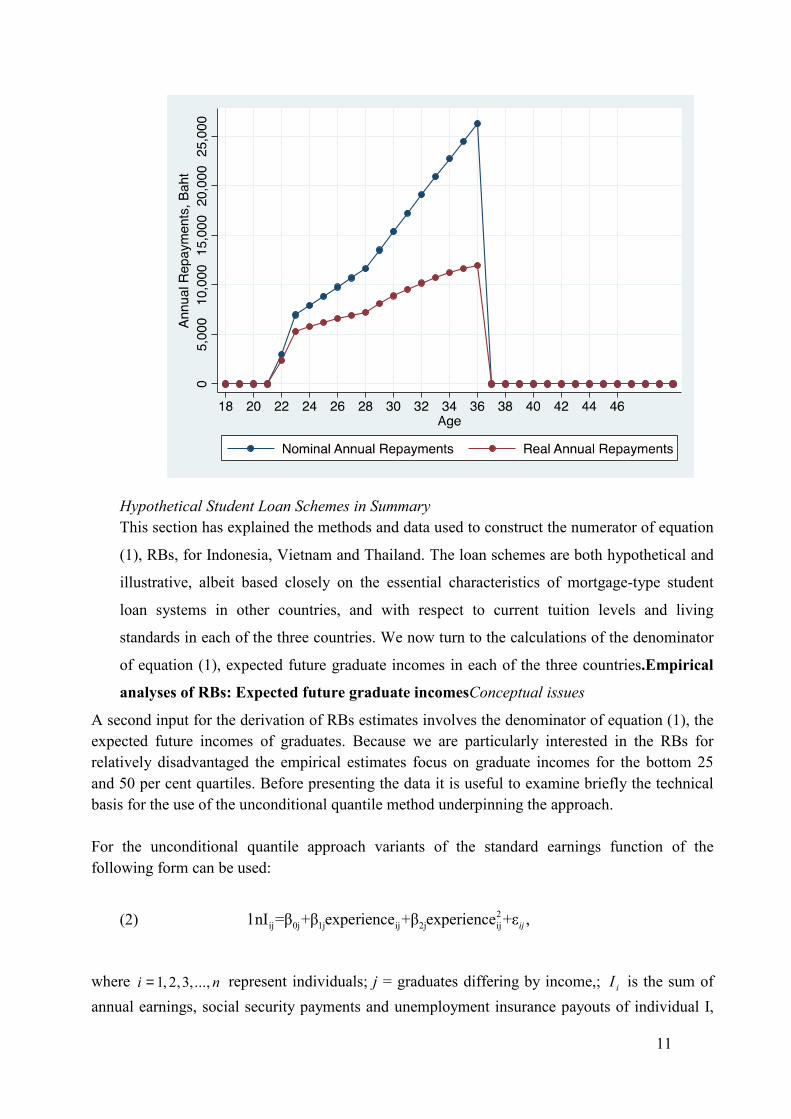
Given these assumed debts and parameters Figure 1 illustrates the annual repayment

obligations for students borrowing in the hypothetical Indonesian student loan system.

Figure 1

Indonesia Hypothetical Loan Repayments

9

The Characteristics of the Loan Scheme: Vietnam

As is the case for Indonesia, currently Vietnam does not have a broadly based higher

education student loans system, and the system now described is again hypothetical but

plausible. As a guide to the characteristics of a “standard” student loans system for

Indonesia, the following features have been assumed: a total debt per student of 32 million

dong, which roughly reflects average tuition charges currently charged in Vietnamese

universities and an estimate for minimal living expenses; a real rate of interest of 3 per cent

per annum, and a repayment period of 10 years. As with the design of the Indonesian

student loan systems these assumptions have been informed by the levels and structures

used in the student loan systems of other countries, such as the US, Canada and Thailand.

Given these assumed debts and parameters Figure 2 illustrates the annual repayment

obligations for students borrowing in the hypothetical Vietnamese student loan system.

Figure 2

Vietnamese Hypothetical Loan Repayments

10

The Characteristics of the Loan Scheme: Thailand

Thailand has had a student loans system, known as the Student Loan Fund (the SLF), in

operation since 1997, and its essential characteristics are used in the loan system designed

for our exercises. These include a 15 year repayment period, with repayments increasing in

both absolute and proportionate terms when the repayment period begins. As well, the

typical SLF loan amount of 300,000 baht has been used. However, as demonstrated in both

Ziderman (2005) and Chapman et al. (2010), the SLF is associated with extremely high

interest rate subsidies, and the hypothetical system now under consideration adjusts for this

subsidy through the use of a real rate of interest of 3 per cent per annum.

Given these assumed debts and parameters Figure 3 illustrates the annual repayment

obligations for students borrowing in the hypothetical Thailand student loan system.

Figure 3

Thailand Hypothetical Loan Repayments

11

Hypothetical Student Loan Schemes in Summary

This section has explained the methods and data used to construct the numerator of equation

(1), RBs, for Indonesia, Vietnam and Thailand. The loan schemes are both hypothetical and

illustrative, albeit based closely on the essential characteristics of mortgage-type student

loan systems in other countries, and with respect to current tuition levels and living

standards in each of the three countries. We now turn to the calculations of the denominator

of equation (1), expected future graduate incomes in each of the three countries.Empirical

analyses of RBs: Expected future graduate incomesConceptual issues

A second input for the derivation of RBs estimates involves the denominator of equation (1), the

expected future incomes of graduates. Because we are particularly interested in the RBs for

relatively disadvantaged the empirical estimates focus on graduate incomes for the bottom 25

and 50 per cent quartiles. Before presenting the data it is useful to examine briefly the technical

basis for the use of the unconditional quantile method underpinning the approach.

For the unconditional quantile approach variants of the standard earnings function of the

following form can be used:

(2) 2

ij 0j 1j ij 2j ijl nI =β +β experience +β experience +ε ,ij

where 1, 2,3,...,i n= represent individuals; j = graduates differing by income,; iI is the sum of

annual earnings, social security payments and unemployment insurance payouts of individual I,

12

differentiated by sex. To capture differences in increases of income with age these are also

interacted with potential experience and its square, defined as:

Experience = age - time to complete a degree – age at which schooling begins

The unconditional quantile regression (UQR) technique is employed to estimate earnings

functions, with this technique being chosen to address the shortcomings associated with the use

of OLS, in two senses. The first is that OLS estimates the mean value conditional on the

distribution of the dependent variable, with a concern arising if the conditional distribution of

dependent variable is skewed, asymmetric, and/or does not have a unique mode. Using OLS

estimates may not give robust results, this problem being common in the context of wage

determination given the asymmetry in wage distributions.8

A second attractive feature of (and the most important reason for us to use) unconditional

quantile regression is that it provides a disaggregated picture of income distributions. This

advantage is crucial to our analysis of student loans since repayment burdens must be highest for

those in the lowest parts of the income distribution (Chapman and Lounkaew, 2010; Chapman et

al., 2010), a feature which cannot be captured by the use of standard OLS. Thus we estimate age-

income profiles for the 25th and 50th (median) quantiles of income distributions by age, with

separate estimations being carried out for males and females.9

The unconditional quantile regression method follows Firpo, Fortin, and Lemieux (2009), a

technique which relies on a transformation known as re-centered influence function (RIF). The

RIF for the quantile of interest, qτ is

(3)

where ( ).If is the marginal density function of I where D is an indicator function. In practice

( ; )RIF I qτ is not observed, hence its sample counterpart is used instead:

(4)

where q̂τ is the sample quantile and ( )ˆIf qτ is the kernel density estimator, with this transformed

variable being used in place of the original dependent variable. One crucial distinguishing feature

of the UQR is that it provides us with a way to recover the marginal impact of the regressors on

the unconditional quantile of I; in the context of this study it is the marginal impact of additional

years of potential experience on income of each income quantile. Usual inference procedures of

the OLS are also applicable to the UQR estimates.

( )( )

( ; ) ,I

D I qRIF I q q

f q

ττ τ

τ

τ − ≤= +

( )ˆ( )

ˆ ˆ( ; ) ,ˆI

D I qRIF I q q

f q

ττ τ

τ

τ − ≤= +

13

In what now follows large household surveys of individuals have been used in each of the four

countries to illustrate graduate annual incomes by age, separately for males and females with

results presented for the bottom 25 and 50 per cent of the graduate income quantils (called Q25

and Q50). Details of the data and econometric results are available in Chapman and Luonkaew

(2010), Chapman et al. (2010), Chapman and Liu (2012) and Chapman and Suryadarma (2012).

Q25 and Q50 graduate age-income profiles: Indonesia

With the use of data and methods explained in Chapman and Suryadarma (2012), age-earnings

profiles have been constructed for Indonesian graduates surveyed in 2009. These exercises allow

the calculation of age-income profiles for both male and female graduates in the bottom 25 and

50 per cent quartiles. These have been estimated for two main Indonesian islands, Java and

Sumatra, chosen because they represent relatively rich and poor Indonesians respectively. The

results are presented in Figure 4.

Figure 4

Male and Female Java and Sumatra Indonesian Graduate Age-Income Profiles: Q25 and

Q50

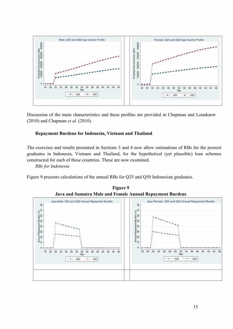
Discussion of the main characteristics and these profiles are provided in Chapman and Suryadarma

(2012).

14

Q25 and Q50 graduate age-income profiles: Vietnam

With the use of data and methods explained in Chapman and Liu (2012), age-earnings profiles

have been constructed for Vietnamese graduates surveyed in 2008. These exercises allow the

calculation of age-income profiles for both male and female graduates in the bottom 25 and 50

per cent quartiles. These have been estimated for both relatively rich urban and relatively poor

rural areas in Vietnam, chosen because these areas allow insights into the ranges of the income

data by region. The results are presented in Figure 5.

Figure 5

Male and Female Rich Urban and Poor Rural Vietnamese Graduate Age-Income Profiles:

Q25 and Q50

Discussion of the main characteristics and these profiles are provided in Chapman and Liu (2012).

Q25 and Q50 graduate age-income profiles: Thailand

With the use of data and methods explained in Chapman and Lounkaew (2010), age-earnings

profiles have been constructed for Thai graduates surveyed in 2008. These exercises allow the

calculation of age-income profiles for both male and female graduates in the bottom 25 and 50

per cent quartiles. The results are presented in Figure 6.

Figure 6

Male and Female Thai Graduate Age-Income Profiles: Q25 and Q50

15

Discussion of the main characteristics and these profiles are provided in Chapman and Lounkaew

(2010) and Chapman et al. (2010).

Repayment Burdens for Indonesia, Vietnam and Thailand

The exercises and results presented in Sections 3 and 4 now allow estimations of RBs for the poorest

graduates in Indonesia, Vietnam and Thailand, for the hypothetical (yet plausible) loan schemes

constructed for each of these countries. These are now examined.

RBs for Indonesia

Figure 9 presents calculations of the annual RBs for Q25 and Q50 Indonesian graduates.

Figure 9

Java and Sumatra Male and Female Annual Repayment Burdens

16

The critical points from Figure 9 are:

(i) For relatively advantaged graduates (Q50, living in Java) the RBs are of the

order of 20-30 per cent per year;

(ii) In the highest income island of Java, graduates in the lowest quartile of

incomes have RBs of the order of 35-60 per cent per year;

(iii) In the low income island of Sumatra, median income graduates face RBs of

the order of 25-40 per cent per year; and

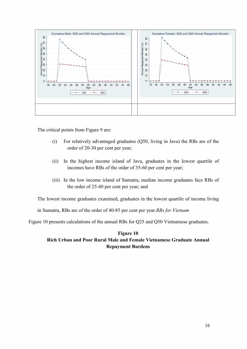
The lowest income graduates examined, graduates in the lowest quartile of income living

in Sumatra, RBs are of the order of 40-85 per cent per year.RBs for Vietnam

Figure 10 presents calculations of the annual RBs for Q25 and Q50 Vietnamese graduates.

Figure 10

Rich Urban and Poor Rural Male and Female Vietnamese Graduate Annual

Repayment Burdens

17

The critical points from Figure 10 are:

(i) For relatively advantaged graduates (Q50, living in urban relatively rich

areas) the RBs are of the order of 15-25 per cent per year;

(ii) In the highest income areas of Vietnam, graduates in the lowest quartile of

incomes have RBs of the order of 20-45 per cent per year;

(iii) In the poorest areas of Vietnam, median income graduates face RBs of the

order of 20-60 per cent per year; and

(iv) The lowest income graduates examined, graduates in the lowest quartile of

income living in the poorest parts of Vietnam, RBs are of the order of 30-80

per cent per year.

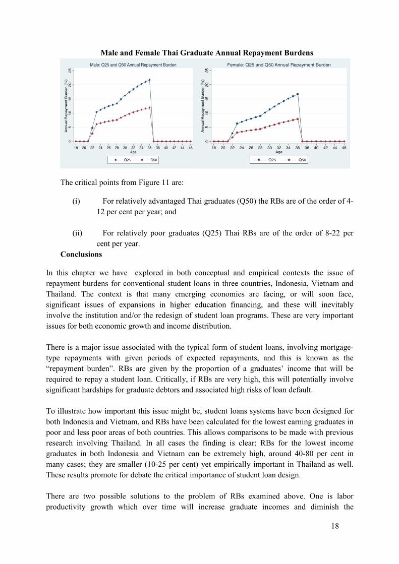
RBs for Thailand

Figure 11 presents calculations of the annual RBs for Q25 and Q50 Vietnamese graduates.

Figure 11

18

Male and Female Thai Graduate Annual Repayment Burdens

The critical points from Figure 11 are:

(i) For relatively advantaged Thai graduates (Q50) the RBs are of the order of 4-

12 per cent per year; and

(ii) For relatively poor graduates (Q25) Thai RBs are of the order of 8-22 per

cent per year.

Conclusions

In this chapter we have explored in both conceptual and empirical contexts the issue of

repayment burdens for conventional student loans in three countries, Indonesia, Vietnam and

Thailand. The context is that many emerging economies are facing, or will soon face,

significant issues of expansions in higher education financing, and these will inevitably

involve the institution and/or the redesign of student loan programs. These are very important

issues for both economic growth and income distribution.

There is a major issue associated with the typical form of student loans, involving mortgage-

type repayments with given periods of expected repayments, and this is known as the

“repayment burden”. RBs are given by the proportion of a graduates’ income that will be

required to repay a student loan. Critically, if RBs are very high, this will potentially involve

significant hardships for graduate debtors and associated high risks of loan default.

To illustrate how important this issue might be, student loans systems have been designed for

both Indonesia and Vietnam, and RBs have been calculated for the lowest earning graduates in

poor and less poor areas of both countries. This allows comparisons to be made with previous

research involving Thailand. In all cases the finding is clear: RBs for the lowest income

graduates in both Indonesia and Vietnam can be extremely high, around 40-80 per cent in

many cases; they are smaller (10-25 per cent) yet empirically important in Thailand as well.

These results promote for debate the critical importance of student loan design.

There are two possible solutions to the problem of RBs examined above. One is labor

productivity growth which over time will increase graduate incomes and diminish the

19

empirical and policy issue of high RBs; the relatively high per capita incomes in Thailand

illustrate that RBs are very sensitive to national productivity levels. However, given the extent

of the current and expected near-future problem, this will only be a medium term solution to

the issue for many countries including Indonesia and Vietnam.

Second, there is a loan scheme which avoids the RB problem, known as income contingent

loans, explained briefly in the Australian context earlier. With ICL the maximum proportion of

a graduate’s income to be used in the repayment of a student loan is set by law (and is, for

example, 8, 9 and 10 per cent of income in Australia, New Zealand and England). But ICL

require a sophisticated loan collection agency, such as a comprehensive internal revenue

service (tax office) and without this type of institution loan repayment leakages are likely to be

high10. The case for both economic growth and governmental institutional reform to help

resolve higher education financing difficulties are incontestable for many emerging economies.

Acknowledgments

The author acknowledges gratefully support from a research grant provided by the Dhurakij

Pundit University/Australian National University research agreement. Important assistance

was provided by Drs Amy Liu and Daniel Suryadarma, excellent research assistance by

Raya Umbu. Conference participants provided useful feedback. The author alone is

responsible for omissions and errors.

References

Baum, S. & Schwartz, S. (2006). How much debt is too much? Defining benchmarks

for manageable student debt. Washington, DC: The College Board.

Chapman, B. (2006). Government managing risk: Income contingent loans for social

and economic progress. London: Routledge.

Chapman, B. and Tim Higgins (2012), “Estimates of foregone HECS repayments from

graduates going overseas”, mimeo, Crawford School, ANU.

Chapman, B. and Kiatanantha Lounkaew (2010a), “Income Contingent Student Loans for

Thailand: Alternatives Compared” (with Kiatanantha Lounkaew), Economics of Education

Review, Vol. 29 (5): 695-709.

Chapman, B. and Kiatanantha Lounkaew (2010b), “Repayment Burdens with US College

Loans”, Centre for Economic Policy Research Discussion Paper No. 647, Research School

of Economics, ANU.

20

Chapman, B. Kiatanantha Lounkaew, Piruna Polsiri, Rangsit Sarachitti, and Thitima

Sitthipongpanich (2010), “Thailand’s Student Loan Fund: An Analysis of Interest Rate

Subsidies and Repayment Hardships”, Economics of Education Review, Vol. 29 (5): 685-

694.

Chapman, B. and Amy Liu (underway, 2012), “Repayment burdens with a Vietnamese

student loan policy”, Crawford School, ANU.

Chapman, B. and Daniel Suryadarma (underway, 2012), “Repayment burdens with an

Indonesian student loan policy”, Crawford School, ANU.

Chapman, B. & Ryan, C. (2002). Income-contingent financing of student charges for higher

education: Assessing the Australian innovation. The Welsh Journal of Education, 11(1),

64-81.

Dynarski, S.M. (1994). Who defaults on student loans: findings from the national

post-secondary student aid study. Economics of Education Review, 13(1), 55-68.

Friedman, M. (1955). The role of government in education. In A. Solo, Economics

and the Public Interest (pp. 123-144). New Brunswick: Rutgers University Press.

Johnstone, D. B. (1986). Sharing the costs of higher education: Student financial

assistance in the United Kingdom, the Federal Republic of Germany, France,

Sweden, and the United States. New York: The College Board.

Salmi, J. (2003). Student loans in an international perspective: The World Bank

experience. Working paper number 27295. Washington, DC: World Bank.

Shen, H. & Ziderman, A. (2007). Student Loans Repayment and Recovery: International

Comparisons. Higher Education, 57(3), 315-333.

Weesakul, B. (2006). Student loans in Thailand: Past, present and future. Mimeo,

Dhurakij Pundit University.

Woodhall, M. (1987). Establishing student loans in developing countries: Some

guidelines. Education and training series discussion paper number EDT 85.

Washington, DC: The World Bank.

Ziderman. A. (2003). Student Loans in Thailand: Are They Effective. Equitable, Sustainable?.

Bangkok: UNESCO.

21

Endnotes

Acknowledgements: Conference participants provided useful feedback, Wendy Dobson in particular. 1 Previous studies have investigated student loan schemes in many countries, for example, Australia (Chapman & Ryan, 2002; Chapman, 2006), Europe and the US (Johnstone, 1986), Africa (Johnstone & Amero, 2001; Johnstone, 2004), South East Asia (Ziderman, 2004) and developing countries more generally (Woodhall, 1987).

2 For analysis of the Australian system, see Chapman (2006). 3 See Woodhall (1987), Ziderman (1999), Schwartz and Finnie (2002), Salmi (2003) and Baum and Schwartz (2006). 4 In the Australian income contingent college loan scheme, for example, the maximum percentage of taxable income of the debt that is repaid is 8 per cent per annum. 5 It is commonly understood that the commercial financing sector will not provide loans to students because of their lack of collateral in the event of default (Friedman, 1955; Barr, 2003; Chapman, 2006). 6 For recent analyses see Ziderman (2003) and Chapman and Lounkaew (2010). 7 For example, Chapman and Lounkaew (2010) found R2 of around 0.4 for Thai earning functions; a plethora of other earnings function studies typically explain no more than 20-30 per cent of the variance. 8Many recent studies have used disaggregated approach to analyse wage distribution and wage determination (Buchinsky, 1994; Machado and Mata, 2001). 9 These profiles have been adjusted using OLS standard errors (see Wooldridge, 2006). 10 Some of the costs of ICL are administrative and discussion is provided in Chapman (2006). Issues of moral hazard, and the issues of emigration matter too (see Chapman and Higgins, 2012).