Higher-order models versus direct hierarchical models: g ...€¦ · Higher-order models versus direct hierarchical models: g as superordinate or breadth factor? 23 he believed the

Psychology Science Quarterly, Volume 50, 2008 (1), p. 21-43

Higher-order models versus direct hierarchical models: g as superordinate or breadth factor?

GILLES E. GIGNAC1

Abstract Intelligence research appears to have overwhelmingly endorsed a superordinate (higher-order

model) conceptualization of g, in comparison to the relatively less well-known breadth conceptualiza-tion of g, as represented by the direct hierarchical model. In this paper, several similarities and distinc-tions between the indirect and direct hierarchical models are delineated. Based on the re-analysis of five correlation matrices, it was demonstrated via CFA that the conventional conception of g as a higher-order superordinate factor was likely not as plausible as a first-order breadth factor. The results are discussed in light of theoretical advantages of conceptualizing g as a first-order factor. Further, because the associations between group-factors and g are constrained to zero within a direct hierarchical model, previous observations of isomorphic associations between a lower-order group factor and g are ques-tioned.

Key words: confirmatory factor analysis, higher-order models, hierarchical models, general intelli-

gence

1 Gilles E. Gignac, School of Psychology, University of Western Australia, 35 Stirling Highway, Crawley,

WA, 6009, Australia; email: [email protected]

G. E. Gignac 22

A non-negligible amount of research has accumulated over the last couple of decades relevant to the examination of the associations between group-factors of intelligence and g. Overwhelmingly, this area of research has tended to employ a higher-order modeling strat-egy within a structural equation modeling (SEM) framework. Much, if not all, of this factor analytic research has neglected to examine specifically the possibility that a breadth concep-tualization of g, as represented by a direct hierarchical model, may be more consistent with the data than a superordinate conceptualization of g, as represented by a higher-order model. Consequently, in this paper, what is referred to as a direct hierarchical model (described more fully below) will be suggested as a plausible alternative to the more conventional higher-order model representation of cognitive abilities. In addition to the theoretical impli-cations of a breadth conceptualization of g, the consequences of finding empirical evidence in favour of the direct hierarchical model over the higher-order model may be viewed as counter evidence against contentions that a lower-order group-factor is isomorphic with g (e.g., Colom et al., 2004; Gustafsson, 1984; Gustafsson, 2001), as the associations between group-factors and g are constrained to zero within a conventional direct hierarchical model. Prior to testing the superordinate versus breadth conceptualizations of g empirically, several of the various terms used to represent particular multi-factor models in intelligence research will be described. In particular, the similarities and distinctions between the higher-order model, the indirect hierarchical model and the direct hierarchical model will be expounded.

Multi-Factor Modeling: some history and nomenclature Although a specific review of the literature does not appear to have ever been conducted,

it would probably be accurate to suggest that the vast majority of factor modeling research in the area of intelligence has implicitly or explicitly endorsed a higher-order factor conceptu-alization of intelligence. In Thurstone’s (1947) Multiple-Factor Analysis, an early and influ-ential factor analytic text in America, a second-order factor conceptualization of g was spe-cifically endorsed: “…a general second-order factor is likely to be of more fundamental significance for the domain in question than a general orthogonal first-order factor,” because the second-order factor is a “participant in the definition of the other [lower-order] factors” (p. 418). More recently, a preference for a higher-order conceptualisation of intelligence persists. For example, Borsboom and Dolan (2006) wrote, “The evidence for the existence of g as a source of individual differences, or, equivalently, as a source of variance, is estab-lished by means of factor analysis of a wide variety of IQ test scores, in which g is identified with the common factor at the apex of a hierarchical common factor model” (p. 434).

An early detractor of the view of g as a higher-order factor was Humphreys (1962) who much preferred what he (and others) referred to as a ‘hierarchical model’. Humphreys (1962) preferred a hierarchical model over a higher-order model for two primary reasons. First, he believed a hierarchical model solution was easier to interpret, because all of the factors were defined by observed variables (i.e., cognitive ability subtests): “Second-order factors are mysterious because they are defined, not by tests, but by first-order factors. Third-order factors are completely incomprehensible” (p. 476). Guilford (1954) shared a similar sceptical view of higher-order factors: “The writer reserves judgment with respect to the psychologi-cal validity of factors higher than the first-order factors” (p. 521). The second reason Hum-phreys (1962) preferred a hierarchical model conceptualization of intelligence was because


23

he believed the key element underpinning the g factor was its breadth rather than its su-perordination, where breadth represented the number of variables which defined a factor and superordination referred to an order greater (“higher”) to that of another.

It will be noted here, however, that when Humphreys (1962) wrote that he preferred a hi-erarchical model over a higher-order model, his preference was in fact not for a distinct model, per se, but a transformation (or reparameterization) of the conventionally conceived higher-order model. In fact, when Humphreys (1962) used the term ‘hierarchical model’ he was referring to the Schmid-Leiman (1957) transformation, which is a procedure that is completely dependent upon the higher-order model solution for its computations (see Gignac, 2007a, for example). McDonald (1999) referred to a Schmid-Leiman transformed solution as an ‘indirect hierarchical model’, which can be distinguished from a ‘direct hierar-chical model’. There are two known approaches to estimating a direct hierarchical model solution. The first method was developed within an unrestricted (“exploratory”) factor ana-lytic framework by Holzinger and Swineford (1937) and is known as the ‘bi-factor method’. The second approach to estimating a direct hierarchical model was developed within a re-stricted (“CFA”) factor analytic framework and was first referred to as a ‘nested factor model’ (Gustafsson and Balke, 1993).2

Although previous researchers such as Thurstone, Humphreys, and others have endorsed particular approaches to estimating and/or interpreting multi-factor models/solutions, the scientific value of these approaches may be questioned, as their preferences were not based on any objective or statistical criteria. That is, because a higher-order model and an indirect hierarchical model (i.e., Schmid-Leiman transformation) are simply alternative representa-tions of the same model (Gignac, 2007a), it is impossible to choose one model over the other, statistically. In contrast, a higher-order model (or indirect hierarchical model) and a direct hierarchical model can be distinguished, statistically (Yung, Thissen, & McLeod, 1999). To help understand why this is the case, it may be beneficial to explain in more detail (and non-technically) the distinctions between a higher-order model and a direct hierarchical model.

Higher-order models and mediation Yung, Thissen, and McLeod (1999) proved analytically that a higher-order model is a

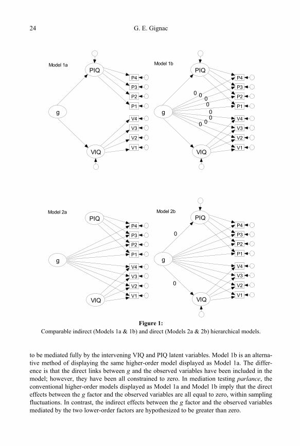
model that implies full mediation. That is, a conventional higher-order model implies that the association between a higher-order factor and the observed variables is mediated fully by the lower-order factors. Model 1a (see Figure 1) depicts a typical higher-order model with a second-order general factor and two first-order factors (VIQ and PIQ), each defined by four observed variables. The mediational nature of higher-order models is perhaps more easily recognized when displayed in a left to right format, rather than the top to bottom format typically used to display higher-order models, graphically. From this perspective, Model 1a specifies that the association between the latent g variable and the eight indicators is implied

2 This assertion is made within the context of intelligence research. Technically, direct hierarchical models

have been used as far back as 1970 within the context of CFA multitrait-multimethod analyses (e.g., Werts & Linn, 1970).

G. E. Gignac 24

g

P4

P3

P2

P1

V4

V3

V2

V1

PIQ

VIQ

g

P4

P3

P2

P1

V4

V3

V2

V1

PIQ

VIQ

0 0 0000

00

g

P4

P3

P2

P1

V4

V3

V2

V1

PIQ

VIQ

g

P4

P3

P2

P1

V4

V3

V2

V1

PIQ

VIQ

0

0

Model 1a Model 1b

Model 2a Model 2b

Figure 1:

Comparable indirect (Models 1a & 1b) and direct (Models 2a & 2b) hierarchical models.

to be mediated fully by the intervening VIQ and PIQ latent variables. Model 1b is an alterna-tive method of displaying the same higher-order model displayed as Model 1a. The differ-ence is that the direct links between g and the observed variables have been included in the model; however, they have been all constrained to zero. In mediation testing parlance, the conventional higher-order models displayed as Model 1a and Model 1b imply that the direct effects between the g factor and the observed variables are all equal to zero, within sampling fluctuations. In contrast, the indirect effects between the g factor and the observed variables mediated by the two lower-order factors are hypothesized to be greater than zero.


25

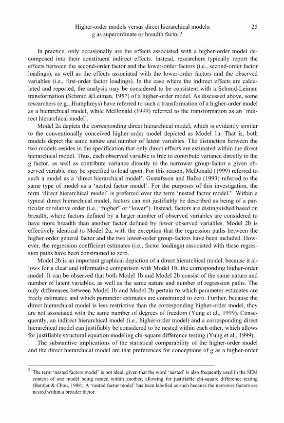
In practice, only occasionally are the effects associated with a higher-order model de-composed into their constituent indirect effects. Instead, researchers typically report the effects between the second-order factor and the lower-order factors (i.e., second-order factor loadings), as well as the effects associated with the lower-order factors and the observed variables (i.e., first-order factor loadings). In the case where the indirect effects are calcu-lated and reported, the analysis may be considered to be consistent with a Schmid-Leiman transformation (Schmid &Leiman, 1957) of a higher-order model. As discussed above, some researchers (e.g., Humphreys) have referred to such a transformation of a higher-order model as a hierarchical model, while McDonald (1999) referred to the transformation as an ‘indi-rect hierarchical model’.

Model 2a depicts the corresponding direct hierarchical model, which is evidently similar to the conventionally conceived higher-order model depicted as Model 1a. That is, both models depict the same nature and number of latent variables. The distinction between the two models resides in the specification that only direct effects are estimated within the direct hierarchical model. Thus, each observed variable is free to contribute variance directly to the g factor, as well as contribute variance directly to the narrower group-factor a given ob-served variable may be specified to load upon. For this reason, McDonald (1999) referred to such a model as a ‘direct hierarchical model’. Gustafsson and Balke (1993) referred to the same type of model as a ‘nested factor model’. For the purposes of this investigation, the term ‘direct hierarchical model’ is preferred over the term ‘nested factor model.’3 Within a typical direct hierarchical model, factors can not justifiably be described as being of a par-ticular or relative order (i.e., “higher” or “lower”). Instead, factors are distinguished based on breadth, where factors defined by a larger number of observed variables are considered to have more breadth than another factor defined by fewer observed variables. Model 2b is effectively identical to Model 2a, with the exception that the regression paths between the higher-order general factor and the two lower-order group-factors have been included. How-ever, the regression coefficient estimates (i.e., factor loadings) associated with these regres-sion paths have been constrained to zero.

Model 2b is an important graphical depiction of a direct hierarchical model, because it al-lows for a clear and informative comparison with Model 1b, the corresponding higher-order model. It can be observed that both Model 1b and Model 2b consist of the same nature and number of latent variables, as well as the same nature and number of regression paths. The only differences between Model 1b and Model 2b pertain to which parameter estimates are freely estimated and which parameter estimates are constrained to zero. Further, because the direct hierarchical model is less restrictive than the corresponding higher-order model, they are not associated with the same number of degrees of freedom (Yung et al., 1999). Conse-quently, an indirect hierarchical model (i.e., higher-order model) and a corresponding direct hierarchical model can justifiably be considered to be nested within each other, which allows for justifiable structural equation modeling chi-square difference testing (Yung et al., 1999).

The substantive implications of the statistical comparability of the higher-order model and the direct hierarchical model are that preferences for conceptions of g as a higher-order

3 The term ‘nested factors model’ is not ideal, given that the word ‘nested’ is also frequently used in the SEM

context of one model being nested within another, allowing for justifiable chi-square difference testing (Bentler & Chou, 1988). A ‘nested factor model’ has been labelled as such because the narrower factors are nested within a broader factor.

G. E. Gignac 26

super-ordinate factor versus a first-order breadth factor can be tested, statistically. Previ-ously, researchers such as Thurston, Humphreys and others could only favour one model over the other based on “non-scientific” preferences, such as ease of interpretation (an ad-vantage that should nonetheless not be understated, Gignac, 2007a). However, the history of confirmatory factor analytic intelligence research appears to have largely assumed that g is best conceptualized as a super-ordinate factor. This assumption may be inaccurate and, con-sequently, should be tested empirically with confirmatory factor analysis (CFA).

Past empirical research Some empirical research has begun to emerge addressing this issue. Based on the MAB,

WAIS-R, and WAIS-III, Gignac (2005a; 2006a; 2006b;) has found some CFA evidence in support of the direct hierarchical model as a superior fitting model, in comparison to a higher-order model. However, intelligence batteries such as the MAB and the Wechsler scales should probably not be considered comprehensive enough to represent all of the pri-mary factors generally acknowledged to exist within the wide spectrum of cognitive abilities (see Carroll, 1993). Consequently, it was considered valuable to potentially replicate the effects on several other correlation matrices.

Specifically, the three correlation matrices within the Colom, Rebollo, Palacios, Juan-Espinosa, & Kyllonen (2004) study, the correlation matrix within the Gustafsson (1984) study, and the Holzinger and Swineford (1939) correlation matrix re-analysed by Gustafsson (2001) were considered relevant for the purposes of re-analysis. The correlation matrices within these three investigations were chosen for three primary reasons: (1) they have been published in widely accessible sources; (2) they incorporate a relatively large array of cogni-tive ability tests; and (3) the results associated with the higher-order modeling of these corre-lation matrices have been interpreted to suggest isomorphic like associations between a lower-order group factor and g. More specifically, Colom et al. reported WM higher-order loadings of 1.04, .90 and .93 on a second-order g factor across all three samples, Gustafsson (1984) reported a Gf loading of 1.04 on a third-order g factor, and, finally, Gustafsson (2001) reported that a lower-order Gf factor had a unity loading on the g factor based on his re-analysis of the Holzinger and Swineford (1939) data.

It should be noted that, based on a higher-order modelling re-analysis of the Colom et al. and the Gustafsson (1984) correlation matrices, Gignac (2007b) suggested caution in the interpretation of past CFA studies which have suggested isomorphic loadings between a lower-order group factor and g, because he found that the reliabilities associated with the corresponding latent variable composite scores were very low (resulting in substantial disat-tenuation effects). Thus, further counter evidence against contentions that a lower-order group-factor is isomorphic with g would be suggested in the event that a direct hierarchical model were found to be more consistent with the data, as all of the group-factor associations with g are constrained to zero within a conventional direct hierarchical model. Therefore, the purpose of this investigation was not only to test the competing theories of superordinate g versus breadth g, but also to examine the possibility that a superior fitting direct hierarchical model would suggest that there may not be any associations between lower-order groups factors and g within a properly specified, well-fitting CFA model, in contradistinction to the evidence reported in Colom et al. (2004), Gustafsson (1984) and Gustafsson (2001).


27

Direct hierarchical models and the examination of the greatest indicators of g Although the conventional direct hierarchical model constrains group-factor associations

with g to zero, it may nonetheless be of interest to determine which type of subtests are the best indicators of g. However, an obvious limitation of the direct hierarchical model is that it does not appear to offer any especially useful method of determining which type of indica-tors are the best measures of g, because all of the factor loadings are based on individual subtests. Consequently, a researcher is effectively left with an examination of the magnitude of individual subtests or the calculation of mean subtest loadings based on theoretically defensible subtest groupings (as performed by Gignac, 2006c, for example). For this reason, direct hierarchical model solutions may be argued to offer little opportunity to take advan-tage of the principle of aggregation (Rushton, Brainard, Pressley, 1983) in this respect.

However, there does exist a SEM technique that allows for both the modeling of a direct hierarchical model, as well as the opportunity to take advantage of the principle of aggrega-tion, simultaneously, for the purposes of evaluating the association between a group of indi-cators and a latent variable such as a g factor. The procedure is based on modeling phantom variables within a SEM framework (Rindskopf, 1984). Within the SEM context of this in-vestigation, a phantom variable was considered to represent a composite variable (i.e., summed scores) from which implied correlations between other elements of a given model (e.g., latent variables) could be estimated. Raykov (1997), Fan (2003), and Gignac (2007b) have demonstrated the utility of SEM and phantom variables for the purposes of estimating internal consistency reliability via the reliability index (i.e., the squared correlation between observed scores and true scores). Thus, it would seem plausible to extend the utility of phan-tom variables to the direct hierarchical modeling case, where the association between a meaningful aggregation of scores (i.e., composite variable) and a latent g variable is of inter-est, for the purposes of determining which type of subtests are the strongest correlates of g (i.e., correlates that are not affected by the disattenuation effects observed within higher-order modeling; see Gignac, 2007b, for a detailed discussion on this issue).

Method Correlation matrices

All analyses were based on the three correlation matrices reported in Colom et al. (2004),

the single correlation matrix reported in Gustafsson (1984), and the single correlation matrix reported in Holzinger and Swineford (1939). As reported in Colom et al., 12 cognitive ability tests were administered to the first sample (N = 198) and 15 tests were administered to the second (N = 203) and third samples (N = 193). For further details, see Colom et al. In the case of Gustafsson (1984), the data were reported to be based on a sample of 981 sixth-grade children. A total of 20 cognitive ability variables were included in the Gustafsson (1984) correlation matrix. Further details can be found in Gustafsson (1984). Finally, the Holzinger and Swineford (1939) correlation matrix (which was re-analysed by Gustafsson, 2001) was based on 301 elementary school children (7th and 8th grades) and 24 cognitive ability sub-tests. Further details can be found in Holzinger and Swineford (1939).

G. E. Gignac 28

Data analytic strategy The first stage of the analyses consisted of testing and evaluating the model-fit associated

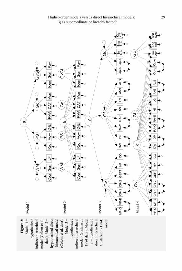
with the higher-order models endorsed by Colom et al. (2004), Gustafsson (1984) and Gustafsson (2001). The sample one higher-order model for the Colom et al. data is depicted in Figure 2 (Model 1). It can be observed that there was one second-order factor (g) and four first-order factors defined by three indicators each. With respect to samples two and three of the Colom et al. data, the higher-order models were modeled very similarly to the sample one higher-order model, with the exception that an additional three observed variables were included in the model to form an additional first-order factor (i.e., Gs). The higher-order model tested on the Gustafsson (1984) data consisted of one first-order g factor and three first-order factors that corresponded to Gv, Gf, and Gc4. Further, correlated residuals were added between the indicators derived from the same subtests to account for the relatively large amount of variance expected to be shared by indicators derived from the same subtest (see Figure 2, Model 3, for a graphical depiction of the Gustafsson (1984) higher-order model). Finally, a higher-order model which corresponded to five first-order factors (Gv, Gc, Gs, Gy, and Gf) and one second-order g factor was tested based on the Holzinger and Swine-ford (1939) data, in accordance with the model tested by Gustafsson (2001). For the pur-poses of scaling/identification, one factor loading from each first-order factor was fixed to 1.0. Further, the higher-order g factor variance was also fixed to 1.0.

Next, the higher-order model solutions were transformed via the Schmid-Leiman proce-dure for the purposes of yielding indirect hierarchical model solutions. As argued by Hum-phreys (1962) and Gignac (2007a), higher-order model solutions should be Schmid-Leiman (1957) transformed into indirect hierarchical model solutions for the purposes of interpreta-tion.

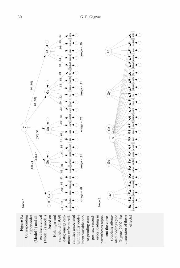
The next subset of analyses consisted of testing the corresponding direct hierarchical models. For the Colom et al. sample one data, the direct hierarchical model consisted of one first-order g factor defined by all 12 subtests and four nested orthogonal first-order factors, corresponding to WM, PS, Gc, and GcGf (see Figure 2, Model 2). The sample two and three direct hierarchical models were specified similarly, with the exception of the addition of a Gs factor defined by an additional three indicators. The Gustafsson (1984) direct hierarchical model consisted of one first-order g factor and three nested group-level factors, correspond-ing to Gv, Gf, and Gc. Further, correlated residuals were added between the indicators de-rived from the same subtests (see Figure 2, Model 4). Finally, the direct hierarchical factor model tested on the Holzinger and Swineford (1939) data consisted of one first-order g fac-tor and five nested, group-level factors (see Figure 3, Model 2). For the purposes of scal-ing/identification, the latent variable variances were constrained to 1.0.

In accordance with Hu and Bentler (1999), a combination approach was used to evaluate model-fit. In this investigation, one absolute close-fit index (SRMR) and two incremental close-fit indices were evaluated (TLI and CFI). Also in accordance with Hu and Bentler (1999), models were evaluated as well-fitting when the SRMR was approximately equal to

4 The higher-order model that was tested in this investigation on the Gustafsson (1984) data had only two-

orders, rather than the three tested in Gustafsson (1984), for the same reasons that were delineated in Gignac (2007b).


29

Figu

re 2

: M

odel

1 =

hy

poth

esiz

ed

indi

rect

hie

rarc

hica

l m

odel

(Col

om e

t al.

data

); M

odel

2 =

hy

poth

esiz

ed d

irect

hi

erar

chic

al m

odel

(C

olom

et a

l. da

ta);

Mod

el 3

=

hypo

thes

ized

in

dire

ct h

iera

rchi

cal

mod

el (G

usta

fsso

n 19

84 d

ata)

; Mod

el

2 =

hypo

thes

ized

di

rect

hie

rarc

hica

l G

usta

fsso

n (1

984)

m

odel

WM

g

Ma

Ach

Eng

Ach

Sw Ach

Op-

eO

p-o

ALS

ANS

LGNS

RA-

ER

A-O

DP

DW

CO

HP

GEF

TC

R-2

CR

-1M

F-E

MF-

O

Gv

Gf

Gc

g

Cou

Sen

LF

PS

Rec

Vow

O-E

Gc

PM

AD

AT

Mon

GvG

f

Iden

Sur

fR

av

WM

Cou

Sen

LF

PS

Rec

Vow

O-E

Gc

PM

AD

AT

Mon

GvG

f

Iden

Sur

fR

av

g

Ma

Ach

Eng

Ach

Sw Ach

Op-

eO

p-o

ALS

ANS

LGN

SR

A-E

RA

-OD

PD

WC

OHP

GE

FTC

R-2

CR

-1M

F-E

MF

-O

Gv

Gf

Gc

g

Mod

el 1

Mod

el 2

Mod

el 3

Mod

el 4

G. E. Gignac 30

Figu

re 3

.: C

orre

spon

ding

hi

gher

-ord

er

(Mod

el 1

) and

di-

rect

hie

rarc

hica

l (M

odel

2) m

odel

s ba

sed

on

Hol

zing

er a

nd

Swin

efor

d (1

939)

da

ta; o

meg

a es

ti-m

ates

refe

r to

reli-

abili

ties a

ssoc

iate

d w

ith th

e fir

st-o

rder

la

tent

var

iabl

e co

r-re

spon

ding

com

-po

site

s; se

cond

-or

der l

oadi

ng in

pa

rent

hese

s rep

re-

sent

the

corr

e-sp

ondi

ng a

ttenu

-at

ed lo

adin

gs (s

ee

Gig

nac,

200

7, fo

r di

scus

sion

of t

hese

ef

fect

s)

g

fig_w

num

figfig

_rob

ject

num

_rw

ord_

rw

ordc

para

grin

fow

ordm

sent

enca

pita

lco

deco

unt

add

arith

reas

serie

spu

zzle

cube

sde

duct

loze

nge

pape

rpe

rcep

Gv

Gc

Gy

Gs

Gf

fig_w

num

figfig

_rob

ject

num

_rw

ord_

rw

ordc

para

grin

fow

ordm

sent

enca

pita

lco

deco

unt

add

arith

reas

serie

spu

zzle

cube

sde

duct

loze

nge

pape

rpe

rcep

Gv

Gc

Gy

Gs

Gf .6

6

g

(.61)

.74 (.6

4) .6

7(.5

0) .5

8.6

3 (.5

3)1.

04 (.

92)

.48

.83

.61

.66

.69

.63

.86

.74

.82

.85

.47

.73

.62

.68

.62

.59

.64

.75

omeg

a =

.67

om

ega

= .9

1

omeg

a =

.75

om

ega

= .7

1

om

ega

= .7

9

Mod

el 1

Mod

el 2

.52

.53

.49

.53

.50


31

or less than .06 and the incremental fit indices (TLI and CFI) were approximately .95 or larger. The normalized residual covariance matrices were also examined for indications of model misfit (i.e., values conspicuously larger than |2.0|).

Model fit comparisons between the higher-order models and the direct hierarchical mod-els were based on two approaches. First, the well-known chi-square difference test was used (Steiger, Shapiro, & Browne, 1985). However, this method may be regarded as excessively powerful, in the same way that the chi-square test of the implied model has been criticized as excessively powerful (e.g., Bentler, 1990). Consequently, a practical significance test was also applied, which was based on the observation of a TLI difference of .010 or more be-tween two competing models (as suggested by Gignac, 2007a). Thus, for example, if model A were associated with a TLI of .940 and model B were associated with a TLI of .950, model B would be considered practically better fitting than model A. Comparisons between TLI values was considered appropriate, because the TLI incorporates a penalty for model complexity (Marsh, Balla, & Hau, 1996). A penalty for model complexity was considered important in this investigation, as all of the direct hierarchical models were associated with fewer degrees of freedom (i.e., larger number of freely estimated parameters) in comparison to the corresponding indirect hierarchical models (i.e., higher-order models). All model solutions were estimated via maximum likelihood estimation (AMOS 5.0).

Finally, in order to take advantage of the principle of aggregation, the direct hierarchical models included phantom variables defined by the respective subtests which corresponded to the hypothesized group-factors (each phantom variable was identified by unit weighted constraints from each indicator; i.e., each regression path was constrained to 1.0; see Gignac, 2007b, for further details on modeling phantom variables). Thus, the association between the composites (i.e., phantom variables) and the first-order g factor could be estimated via their respective implied correlations. This procedure is predicated upon the same SEM technique employed by Fan (2003), Raykov (1997) and Gignac (2007b), where phantom modeling was used for the purposes of estimating the reliability index via the implied correlation between a phantom composite variable and its corresponding latent variable (see Fan, 2003, for a non-technical discussion of phantom variable modeling with AMOS). Conceptually, the implied correlation between a phantom composite and a latent g variable may be viewed in a similar manner to the correlation between summed composite scores and g factor scores. Note that in order to obtain the appropriate standardized implied correlations, it was necessary to spec-ify all observed variable variances to 1.0 within the SPSS correlation matrix.

Results Hypothesized higher-order models versus direct hierarchical models

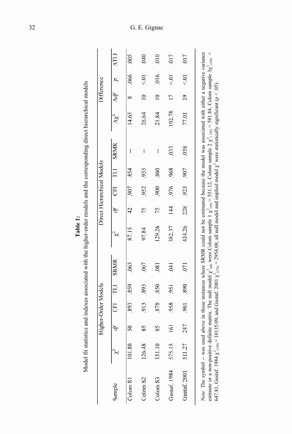
For the purposes of simplicity and clarity, the fit statistics and close-fit indexes associ-

ated with the higher-order models and the direct hierarchical models are all reported in Table 1. It can be observed that only one of the higher-order models (i.e., Gustaf. 1984) was asso-ciated with acceptable levels of model close-fit. In comparison, two of the direct hierarchical models were associated with acceptable levels of model close-fit (i.e., Gustaf. 1984 and Colom S2). More importantly, however, four out of five of the direct hierarchical models

G. E. Gignac 32

Tab

le 1

: M

odel

fit s

tatis

tics a

nd in

dexe

s ass

ocia

ted

with

the

high

er-o

rder

mod

els a

nd th

e co

rres

pond

ing

dire

ct h

iera

rchi

cal m

odel

s

Not

e. T

he s

ymbo

l --

was

use

d ab

ove

in th

ose

inst

ance

s w

here

SR

MR

cou

ld n

ot b

e es

timat

ed b

ecau

se th

e m

odel

was

ass

ocia

ted

with

eith

er a

neg

ativ

e va

rianc

e es

timat

e or

a n

on-p

ositi

ve d

efin

ite m

atrix

. The

nul

l mod

el χ

2 (df) w

ere

Col

om s

ampl

e 1 χ2 (5

0) =

551

.12,

Col

om s

ampl

e 2 χ2 (

105)

= 5

81.8

4, C

olom

sam

ple

3χ2 (1

05) =

64

7.81

, Gus

taf.

1984

χ2 (1

90) =

101

35.0

9, a

nd G

usta

f. 20

01 χ

2 (276

) = 2

954.

08; a

ll nu

ll m

odel

and

impl

ied

mod

el χ

2 w

ere

stat

istic

ally

sign

ifica

nt (p

< .0

5).


33

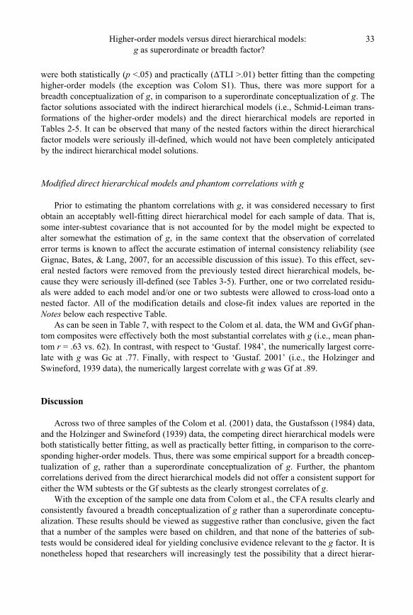
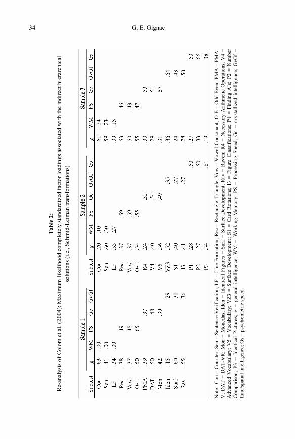
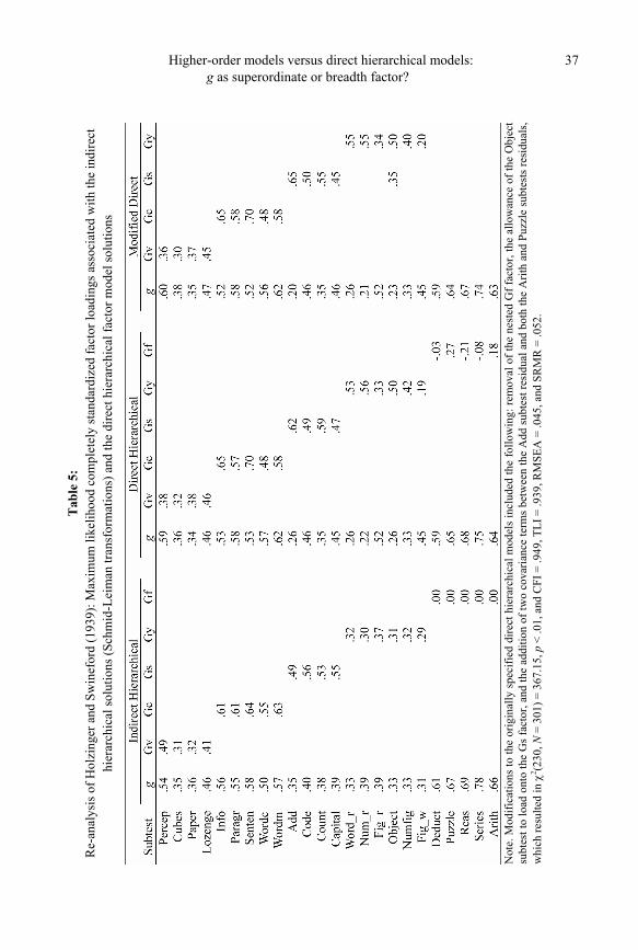
were both statistically (p <.05) and practically (∆TLI >.01) better fitting than the competing higher-order models (the exception was Colom S1). Thus, there was more support for a breadth conceptualization of g, in comparison to a superordinate conceptualization of g. The factor solutions associated with the indirect hierarchical models (i.e., Schmid-Leiman trans-formations of the higher-order models) and the direct hierarchical models are reported in Tables 2-5. It can be observed that many of the nested factors within the direct hierarchical factor models were seriously ill-defined, which would not have been completely anticipated by the indirect hierarchical model solutions.

Modified direct hierarchical models and phantom correlations with g Prior to estimating the phantom correlations with g, it was considered necessary to first

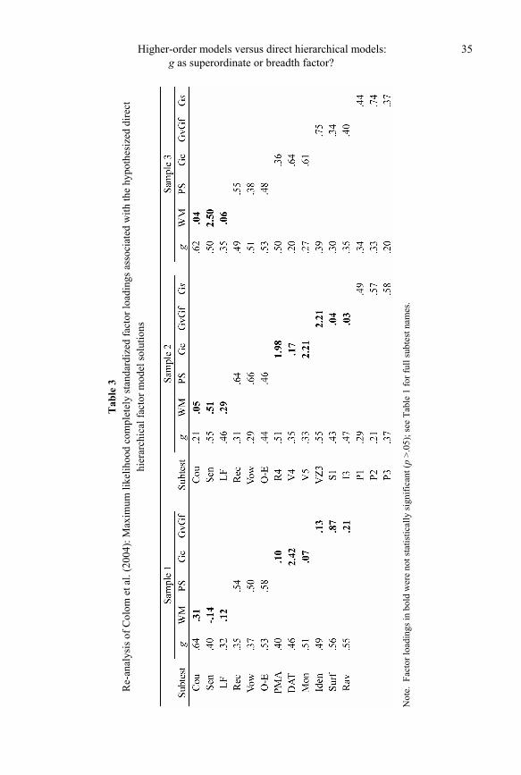
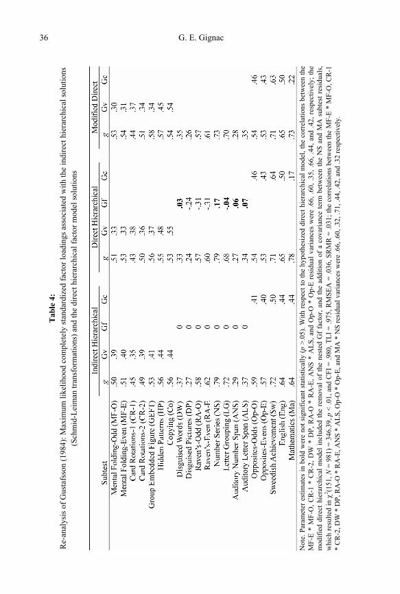
obtain an acceptably well-fitting direct hierarchical model for each sample of data. That is, some inter-subtest covariance that is not accounted for by the model might be expected to alter somewhat the estimation of g, in the same context that the observation of correlated error terms is known to affect the accurate estimation of internal consistency reliability (see Gignac, Bates, & Lang, 2007, for an accessible discussion of this issue). To this effect, sev-eral nested factors were removed from the previously tested direct hierarchical models, be-cause they were seriously ill-defined (see Tables 3-5). Further, one or two correlated residu-als were added to each model and/or one or two subtests were allowed to cross-load onto a nested factor. All of the modification details and close-fit index values are reported in the Notes below each respective Table.

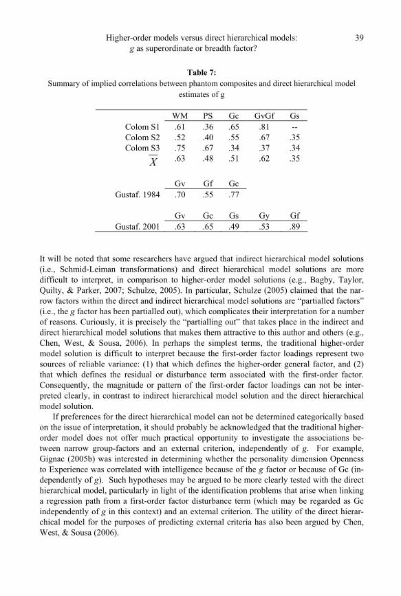
As can be seen in Table 7, with respect to the Colom et al. data, the WM and GvGf phan-tom composites were effectively both the most substantial correlates with g (i.e., mean phan-tom r = .63 vs. 62). In contrast, with respect to ‘Gustaf. 1984’, the numerically largest corre-late with g was Gc at .77. Finally, with respect to ‘Gustaf. 2001’ (i.e., the Holzinger and Swineford, 1939 data), the numerically largest correlate with g was Gf at .89.

Discussion Across two of three samples of the Colom et al. (2001) data, the Gustafsson (1984) data,

and the Holzinger and Swineford (1939) data, the competing direct hierarchical models were both statistically better fitting, as well as practically better fitting, in comparison to the corre-sponding higher-order models. Thus, there was some empirical support for a breadth concep-tualization of g, rather than a superordinate conceptualization of g. Further, the phantom correlations derived from the direct hierarchical models did not offer a consistent support for either the WM subtests or the Gf subtests as the clearly strongest correlates of g.

With the exception of the sample one data from Colom et al., the CFA results clearly and consistently favoured a breadth conceptualization of g rather than a superordinate conceptu-alization. These results should be viewed as suggestive rather than conclusive, given the fact that a number of the samples were based on children, and that none of the batteries of sub-tests would be considered ideal for yielding conclusive evidence relevant to the g factor. It is nonetheless hoped that researchers will increasingly test the possibility that a direct hierar-

G. E. Gignac 34

Tab

le 2

: R

e-an

alys

is o

f Col

om e

t al.

(200

4): M

axim

um li

kelih

ood

com

plet

ely

stan

dard

ized

fact

or lo

adin

gs a

ssoc

iate

d w

ith th

e in

dire

ct h

iera

rchi

cal

solu

tions

(i.e

., Sc

hmid

-Lei

man

tran

sfor

mat

ions

)

Not

e. C

ou =

Cou

nter

; Sen

= S

ente

nce

Ver

ifica

tion;

LF

= Li

ne F

orm

atio

n; R

ec =

Rec

tang

le-T

riang

le; V

ow =

Vow

el-C

onso

nant

; O-E

= O

dd-E

ven;

PM

A =

PM

A-

V; D

AT

= D

AT-

VR

; Mon

= M

oned

as; I

den

= Id

entic

al F

igur

es =

Sur

f =

Surf

ace

Dev

elop

men

t; R

av =

Rav

en; R

4 =

Nec

essa

ry A

rithm

etic

Ope

ratio

ns; V

4 =

Adv

ance

d V

ocab

ular

y; V

5 =

Voc

abul

ary;

VZ3

= S

urfa

ce D

evel

opm

ent;

S1 =

Car

d R

otat

ions

; I3

= F

igur

e C

lass

ifica

tions

; P1

= F

indi

ng A

’s;

P2 =

Num

ber

Com

paris

on;

P3 =

Ide

ntic

al P

ictu

res;

g =

gen

eral

int

ellig

ence

; W

M =

Wor

king

Mem

ory;

PS

= Pr

oces

sing

Spe

ed;

Gc

= cr

ysta

llize

d in

telli

genc

e; G

vGf

= flu

id/s

patia

l int

ellig

ence

; Gs =

psy

chom

etric

spee

d.


35

Tab

le 3

R

e-an

alys

is o

f Col

om e

t al.

(200

4): M

axim

um li

kelih

ood

com

plet

ely

stan

dard

ized

fact

or lo

adin

gs a

ssoc

iate

d w

ith th

e hy

poth

esiz

ed d

irect

hi

erar

chic

al fa

ctor

mod

el so

lutio

ns

Not

e. F

acto

r loa

ding

s in

bold

wer

e no

t sta

tistic

ally

sign

ifica

nt (p

>.0

5); s

ee T

able

1 fo

r ful

l sub

test

nam

es.

G. E. Gignac 36 T

able

4:

Re-

anal

ysis

of G

usta

fsso

n (1

984)

: Max

imum

like

lihoo

d co

mpl

etel

y st

anda

rdiz

ed fa

ctor

load

ings

ass

ocia

ted

with

the

indi

rect

hie

rarc

hica

l sol

utio

ns

(Sch

mid

-Lei

man

tran

sfor

mat

ions

) and

the

dire

ct h

iera

rchi

cal f

acto

r mod

el so

lutio

ns

Not

e. P

aram

eter

est

imat

es in

bol

d w

ere

not s

igni

fican

t sta

tistic

ally

(p >

.05)

. With

resp

ect t

o th

e hy

poth

esiz

ed d

irect

hie

rarc

hica

l mod

el, t

he c

orre

latio

ns b

etw

een

the

MF-

E *

MF-

O, C

R-1

* C

R-2

, DW

* D

P, R

A-O

* R

A-E

, AN

S *

ALS

, and

Op-

O *

Op-

E re

sidu

al v

aria

nces

wer

e .6

6, .6

0, .3

5, .6

6, .4

4, a

nd .4

2, r

espe

ctiv

ely;

the

mod

ified

dire

ct h

iera

rchi

cal m

odel

incl

uded

the

rem

oval

of

the

nest

ed G

f fa

ctor

, and

the

addi

tion

of a

cov

aria

nce

term

bet

wee

n th

e N

S an

d M

A s

ubte

st r

esid

uals

, w

hich

resu

lted

in χ

2 (151

, N =

981

) = 3

46.3

9, p

< .0

1, a

nd C

FI =

.980

, TLI

= .9

75, R

MSE

A =

.036

, SR

MR

= .0

31; t

he c

orre

latio

ns b

etw

een

the

MF-

E *

MF-

O, C

R-1

*

CR

-2, D

W *

DP,

RA

-O *

RA

-E, A

NS

* A

LS, O

p-O

* O

p-E,

and

MA

* N

S re

sidu

al v

aria

nces

wer

e .6

6, .6

0, .3

2, .7

1, .4

4, .4

2, a

nd .3

2 re

spec

tivel

y.


37

Tab

le 5

: R

e-an

alys

is o

f Hol

zing

er a

nd S

win

efor

d (1

939)

: Max

imum

like

lihoo

d co

mpl

etel

y st

anda

rdiz

ed fa

ctor

load

ings

ass

ocia

ted

with

the

indi

rect

hi

erar

chic

al so

lutio

ns (S

chm

id-L

eim

an tr

ansf

orm

atio

ns) a

nd th

e di

rect

hie

rarc

hica

l fac

tor m

odel

solu

tions

Not

e. M

odifi

catio

ns to

the

orig

inal

ly s

peci

fied

dire

ct h

iera

rchi

cal m

odel

s in

clud

ed th

e fo

llow

ing:

rem

oval

of t

he n

este

d G

f fac

tor,

the

allo

wan

ce o

f the

Obj

ect

subt

est t

o lo

ad o

nto

the

Gs

fact

or, a

nd th

e ad

ditio

n of

two

cova

rianc

e te

rms

betw

een

the

Add

subt

est r

esid

ual a

nd b

oth

the

Arit

h an

d Pu

zzle

subt

ests

resi

dual

s, w

hich

resu

lted

in χ

2 (230

, N =

301

) = 3

67.1

5, p

< .0

1, a

nd C

FI =

.949

, TLI

= .9

39, R

MSE

A =

.045

, and

SR

MR

= .0

52.

G. E. Gignac 38

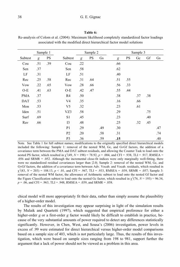
Table 6: Re-analysis of Colom et al. (2004): Maximum likelihood completely standardized factor loadings

associated with the modified direct hierarchical factor model solutions

Sample 1 Sample 2 Sample 3 Subtest g PS Subtest g PS Gs g PS Gc Gf Gs

Cou .51 .39 Cou .22 .66 Sen .37 Sen .58 .62 LF .31 LF .51 .40 Rec .25 .58 Rec .31 .64 .51 .55 Vow .22 .65 Vow .28 .66 .56 .33 O-E .41 .63 O-E .42 .47 .55 .44 PMA .37 R4 .50 .38 .37 .38 DAT .53 V4 .35 .16 .66 Mon .53 V5 .32 .23 .61 Iden .51 VZ3 .58 .29 .75 Surf .69 S1 .45 .23 .40 Rav .66 I3 .48 .25 .32 .45

P1 .29 .49 .30 .47 P2 .20 .58 .31 .74 P3 .36 .59 .15 .40

Note. See Table 1 for full subtest names; modifications to the originally specified direct hierarchical models included the following: Sample 1: removal of the nested WM, Gc, and GvGf factors, the addition of a covariance term between the PMA and DAT subtest residuals, and allowing the Counter Task to load onto the nested PS factor, which resulted in χ2(49, N = 198) = 78.92, p = .004, and CFI = .938, TLI = .917, RMSEA = .056 and SRMR = .052. Although the incremental close-fit indices were only marginally well-fitting, there were no standardized residual covariances larger than |2.0|; Sample 2: removal of the nested WM, Gc, and GvGf factors, the addition of a covariance term between Adv. Vocab. and Vocab. residuals, which resulted in χ2(83, N = 203) = 108.13, p < .01, and CFI = .947, TLI = .933, RMSEA = .039, SRMR = .057; Sample 3: removal of the nested WM factor, the allowance of Arithmetic subtest to load onto the nested Gf factor and the Figure Classification subtest to load onto the nested Gc factor, which resulted in χ2(76, N = 193) = 96.34, p = .06, and CFI = .963, TLI = .948, RMSEA = .039, and SRMR = .058. chical model will more appropriately fit their data, rather than simply assume the plausibility of a higher-order model.

The results of this investigation may appear surprising in light of the simulation results by Mulaik and Quartetti (1997), which suggested that empirical preference for either a higher-order g or a first-order g factor would likely be difficult to establish in practice, be-cause of the very substantial amounts of power required to detect any differences statistically significantly. However, in Chen, West, and Sousa’s (2006) investigation, power levels in excess of .99 were estimated for direct hierarchical versus higher-order model comparisons based on a sample size of 403, which is not particularly large. Thus, the results of this inves-tigation, which were based on sample sizes ranging from 198 to 981, support further the argument that a lack of power should not be viewed as a problem in this area.


39

Table 7: Summary of implied correlations between phantom composites and direct hierarchical model

estimates of g

WM PS Gc GvGf Gs Colom S1 .61 .36 .65 .81 -- Colom S2 .52 .40 .55 .67 .35 Colom S3 .75 .67 .34 .37 .34

X .63 .48 .51 .62 .35

Gv Gf Gc

Gustaf. 1984 .70 .55 .77 Gv Gc Gs Gy Gf

Gustaf. 2001 .63 .65 .49 .53 .89

It will be noted that some researchers have argued that indirect hierarchical model solutions (i.e., Schmid-Leiman transformations) and direct hierarchical model solutions are more difficult to interpret, in comparison to higher-order model solutions (e.g., Bagby, Taylor, Quilty, & Parker, 2007; Schulze, 2005). In particular, Schulze (2005) claimed that the nar-row factors within the direct and indirect hierarchical model solutions are “partialled factors” (i.e., the g factor has been partialled out), which complicates their interpretation for a number of reasons. Curiously, it is precisely the “partialling out” that takes place in the indirect and direct hierarchical model solutions that makes them attractive to this author and others (e.g., Chen, West, & Sousa, 2006). In perhaps the simplest terms, the traditional higher-order model solution is difficult to interpret because the first-order factor loadings represent two sources of reliable variance: (1) that which defines the higher-order general factor, and (2) that which defines the residual or disturbance term associated with the first-order factor. Consequently, the magnitude or pattern of the first-order factor loadings can not be inter-preted clearly, in contrast to indirect hierarchical model solution and the direct hierarchical model solution.

If preferences for the direct hierarchical model can not be determined categorically based on the issue of interpretation, it should probably be acknowledged that the traditional higher-order model does not offer much practical opportunity to investigate the associations be-tween narrow group-factors and an external criterion, independently of g. For example, Gignac (2005b) was interested in determining whether the personality dimension Openness to Experience was correlated with intelligence because of the g factor or because of Gc (in-dependently of g). Such hypotheses may be argued to be more clearly tested with the direct hierarchical model, particularly in light of the identification problems that arise when linking a regression path from a first-order factor disturbance term (which may be regarded as Gc independently of g in this context) and an external criterion. The utility of the direct hierar-chical model for the purposes of predicting external criteria has also been argued by Chen, West, & Sousa (2006).

G. E. Gignac 40

Some may argue that the higher-order model is simpler than the direct hierarchical model, and, consequently, should be preferred on that basis, all other things being equal. However, there may be a counter-argument to this contention. Consider that a higher-order modeling conceptualization of intelligence implies that all of the common variance between subtests from different group-level factors (i.e., factors narrower than g) within a model is due solely to the association between the narrow group-factors (i.e., full mediation). Theo-retically, on what basis may one defend the implication of full mediation implied by the higher-order model? From this perspective, the direct hierarchical model may be considered simpler than the higher-order model, despite the fact that it is associated with fewer degrees of freedom, because it does not require a theoretical justification for full mediation.

Support for the direct hierarchical model of intelligence may also be viewed as consistent with the developmental differentiation hypothesis proposed by Garrett (1946), which con-tends that individual differences in intelligence in children are determined by the general factor, exclusively. During the course of development, various groups of abilities begin to differentiate themselves from g, resulting in a reduction in the dominance of the g factor and the emergence of group-factors. In light of Garret’s (1946) developmental differentiation hypothesis, a higher-order conceptualization of intelligence in adults would imply that the nature of g changes over time such that the effects of g on the association between individual subtests disappears, and is replaced by a g factor that is defined exclusively by the inter-correlations between group-factors. It is argued, here, that the law of parsimony would fa-vour a developmental theory of intelligence consistent with a g factor model that does not change its factor definition over time. Stated simply, on what theoretical basis should the nature of g be described as consistent with a change from direct effects to indirect effects?

Note that a direct hierarchical model does not preclude correlations between group-factors. It is possible to model covariance links between nested factors within a direct hierar-chical model (e.g., Gignac, 2006a). In this investigation, however, there were no indications that any of the nested group-factors should be correlated. Further, it is also possible to model ‘hybrid models’ which incorporate both direct and indirect effects between the indicators and a higher-order general factor (Yung et al., 1999), although the theoretical implications of such a model remain to be established. In fact, it would be expected that there are several models which could have been demonstrated to be associated with acceptable levels of model fit based on the Colom et al. (2004), Gustafsson (1984) and Holzinger and Swineford (1939) data that were not tested in this investigation (see Tomarken & Waller, 2003, for a discussion of the problem of equivalent and non-equivalent models).

Based on the phantom variable modeling strategy, the modified direct hierarchical mod-els of the Colom et al. data suggested that both the WM and GvGf phantom composites were associated with the g factor to effectively the same degree (i.e., .63 vs. .62). With re-spect to the Gustafsson’s data, the phantom composite most greatly associated with g was Gc at .77. Finally, with respect to the Holzinger and Swineford (1939) data, Gf was associated with the strongest correlation (.89) with g. Thus, the implied correlations between the corre-sponding group-factor composites (i.e., phantom variables) and g did not suggest any clear subtest grouping as the strongest correlate of g. These results suggest that there is no firm evidence for a single determinant of g; instead, g appears to be a complex construct defined by multiple determinants, the nature of which may vary somewhat from sample to sample (and subtest battery to subtest battery), resulting in the observation of different greatest indi-cators of g.


41

Another consideration in the evaluation of factor model solutions within the context of the greatest indicator of g debate relates to the fact that not all subtests included in a battery would be expected to contain the same number of items and/or the same number of items representing the same spectrum of item difficulty. For instance, both Vocabulary (Wechsler scales) and Raven’s Progressive Matrices are often found to be the highest loading subtest on a general factor of intelligence (Jensen, 1998). While theories of intelligence may be devel-oped to account for this phenomenon, a simpler possible explanation relates to the fact that both Vocabulary and Raven’s contain a relatively large number of, arguably, high quality items, covering a wide spectrum of item difficulty, in comparison to other subtests often included in a battery of cognitive ability tests (e.g., Picture Completion and Picture Ar-rangement). This fact raises the question as to whether meaningful comparisons can be made between subtests g loadings (or lower-order group factor loadings), even in the case where the loadings have been disattenuated for imperfect reliability. Ultimately, although correc-tions can be made for differences in subtest score reliability, there do not appear to be any established corrections that can be made for differences in subtest validity. Ideally, a defen-sible and valid factor analysis would be based on scores derived from a battery of subtests that represent the same level of validity as an indicator of that narrow element of cognitive ability. Only then would fully meaningful comparisons between factor loadings be possible (or phantom composite correlations). This issue would be expected to require a substantial amount of item level psychometric research to overcome in practice, and, consequently, it is somewhat doubtful that convincing empirical evidence will emerge, in the near future, to indicate which narrow type of cognitive ability factor (or subtest) is the greatest indicator of g. In the event that such an ideal set of data were to emerge, it is recommended that this investigation include analyses relevant to the higher-order model solution, the indirect hier-archical model solution, and the direct hierarchical model solution.

References

Bagby, R. M., Taylor, G. J., Quilty, L. C., & Parker, J. D. A. (2007). Reexamining the factor structure of the 20-item Toronto Alexithymia Scale: Commentary on Gignac, Palmer, and Stough. Journal of Personality Assessment, 89, 258-264.

Bentler, P. M. (1990). Comparative fit indexes in structural models. Psychological Bulletin, 107, 238-246.

Borsboom, D., & Dolan, C. V. (2006). Why g is not an adaptation: A comment on Kanazawa (2004). Psychological Review, 113, 433-437.

Carroll, J. B. (1993). Human cognitive abilities: A survey of factor analytic studies. Cambridge, UK: Cambridge University Press.

Chen, F. F., West, S. G., & Sousa, K. H. (2006). A comparison of bifactor and second-order models of quality of life. Multivariate Behavioral Research, 41, 189-225.

Colom, R., Rebollo, I., Palacios, A., Juan-Espinosa, M., & Kyllonen, P. C. (2004). Working memory is (almost) perfectly predicted by g. Intelligence, 32, 277-296.

Fan, X. (2003). Using commonly available software for bootstrapping in both substantive and measurement analyses. Educational and Psychological Measurement, 63, 24-50.

Garrett (1946). A developmental theory of intelligence. The American Psychologist, 1, 372-378. Gignac, G. E. (2005a). Revisiting the factor structure of the WAIS-R: Insights through nested

factor modeling. Assessment, 12(3), 320-329.

G. E. Gignac 42

Gignac, G. E. (2005b). Openness to experience, general intelligence and crystallized intelligence: A methodological extension. Intelligence, 33, 161-167.

Gignac, G. E. (2006a). A confirmatory examination of the factor structure of the Multidimen-sional Aptitude Battery (MAB): Contrasting oblique, higher-order, and nested factor models. Educational and Psychological Measurement, 66(1), 136-145.

Gignac, G. E. (2006b). The WAIS-III as a nested factors model: A useful alternative to the more conventional oblique and higher-order models. Journal of Individual Differences, 27, 73-86.

Gignac, G. E. (2006c). Evaluating subtest ‘g’ saturation levels via the Single Trait-Correlated Uniqueness (STCU) SEM approach: Evidence in favour of crystallized subtests as the best indicators of ‘g’. Intelligence, 34, 29-46.

Gignac, G. E. (2007a).Multi-factor modeling in individual differences research: Some sugges-tions and recommendations. Personality and Individual Differences, 42, 37-48.

Gignac, G. E. (2007b). Working memory and fluid intelligence are both identical to g?! Reanaly-ses and critical evaluation. Psychology Science, 49, 187-207.

Gignac, G. E., Bates, T. C., Lang, K. (2007). Implications relevant to CFA model misfit, reliabil-ity, and the five-factor model as measured by the NEO-FFI. Personality and Individual Dif-ferences, 43, 1051-1062.

Gustafsson, J-E. (1984). A unifying model for the structure of intellectual abilities. Intelligence, 8, 179-203.

Gustafsson, J-E. (2001). On the hierarchical structure of ability and personality. In J. M. Collis & S. Messick (Eds.), Intelligence and personality: Bridging the gap in theory and measurement (pp. 25-42). Mahwah, NJ: Erlbaum.

Gustafsson, J., & Balke, G. (1993). General and specific abilities as predictors of school achieve-ment. Multivariate Behavioral Research, 28, 407-434.

Holzinger, K. J., & Swineford, F. (1937). The bi-factor method. Psychometrika, 2, 42-54. Holzinger, K. J., & Swineford, F. (1939). A study in factor analysis: The stability of a bi-factor

solution. Supplementary Educational Monographs Vol. 48. Chicago: Department of Educa-tion, University of Chicago.

Hu, L., & Bentler, P. M. (1999). Cutoff criteria for fit indexes in covariance structure analysis: Conventional criteria versus new alternatives. Structural Equation Modeling, 6(1), 1-55.

Humphreys, L. G. (1962). The organization of human abilities. American Psychologist, 17, 475-483.

Jensen, A. R. (1998). The g factor: The science of mental ability. Westport: Praeger. MacCallum, R. C., Wegener, D. T., Uchino, B. N., & Fabrigar, L. R.(1993). The problem of

equivalent models in applications of covariance structure analysis. Psychological Bulletin, 114, 185-199.

Marsh, H. W., Balla, J. W., & Hau, K. (1996). An evaluation of incremental fit indices: A clarifi-cation of mathematical and empirical properties. In G. A. Marcoulides and R. E. Schumacker (Eds.), Advanced structural equation modeling: Issues and techniques (pp. 315-353). Mah-wah, NJ: Erlbaum.

McDonald, R. (1999). Test theory: A unified treatment. Mahwah, NJ: Erlbaum Associates. Raykov, T. (1997). Estimation of composite reliability for congeneric measures. Applied Psycho-

logical Measurement, 21, 173-184. Rindskopf, D. (1984). Using phantom and imaginary latent variables to parameterize constraints

in linear structural models. Psychometrika, 49, 37-47. Rushton, J. P., Brainerd, C. J., & Pressley, M. (1983). Behavioral development and construct

validity: The principle of aggregation. Psychological Bulletin, 94, 18-38.


43

Schmid, J., & Leiman, J. M. (1957). The development of hierarchical factor solutions. Psycho-metrika, 22, 53-61.

Schulze, R. (2005). Modeling structures of intelligence. In O. Wilhelm & R. W. Engle (Eds.), Handbook of understanding and measuring intelligence (pp. 241-263). Thousand Oaks, CA: Sage.

Steiger, J. H., Shapiro, A.,&Browne, M.W. (1985). On the asymptotic distribution of sequential chi-square statistics. Psychometrika, 50, 253-264.

Thurstone, L., L. (1947). Multiple factor analysis. Chicago: University of Chicago Press. Tomarken A. J., & Waller N. G.(2003). Potential problems with “well-fitting” models. Journal of

Abnormal Psychology, 112, 578-598. Werts, C. E., & Linn, R. L. (1970). Path analysis: Psychological examples. Psychological Bulle-

tin, 74, 193-212. Yung, Y-F, Thissen, D., McLeod, L. (1999). On the relationship between the higher-order factor

model and the hierarchical factor model. Psychometrika, 64(2), 113-128.

Documents

Higher-order models versus direct hierarchical models: g ...€¦ · Higher-order models versus direct hierarchical models: g as superordinate or breadth factor? 23 he believed the