1

Higher-Order Partial Least Squares (HOPLS):A Generalized Multi-Linear Regression Method

Qibin Zhao, Cesar F. Caiafa, Danilo P. Mandic, Zenas C. Chao, Yasuo Nagasaka, Naotaka Fujii,Liqing Zhang and Andrzej Cichocki

Abstract—A new generalized multilinear regression model, termed the Higher-Order Partial Least Squares (HOPLS), is introducedwith the aim to predict a tensor (multiway array) Y from a tensor X through projecting the data onto the latent space and performingregression on the corresponding latent variables. HOPLS differs substantially from other regression models in that it explains the databy a sum of orthogonal Tucker tensors, while the number of orthogonal loadings serves as a parameter to control model complexityand prevent overfitting. The low dimensional latent space is optimized sequentially via a deflation operation, yielding the best jointsubspace approximation for both X and Y. Instead of decomposing X and Y individually, higher order singular value decompositionon a newly defined generalized cross-covariance tensor is employed to optimize the orthogonal loadings. A systematic comparisonon both synthetic data and real-world decoding of 3D movement trajectories from electrocorticogram (ECoG) signals demonstratethe advantages of HOPLS over the existing methods in terms of better predictive ability, suitability to handle small sample sizes, androbustness to noise.

Index Terms—Multilinear regression, Partial least squares (PLS), Higher-order singular value decomposition (HOSVD), Constrainedblock Tucker decomposition, Electrocorticogram (ECoG), Fusion of behavioral and neural data.

F

1 INTRODUCTION

THE Partial Least Squares (PLS) is a well-establishedframework for estimation, regression and classifica-

tion, whose objective is to predict a set of dependentvariables (responses) from a set of independent variables(predictors) through the extraction of a small number oflatent variables. One member of the PLS family is PartialLeast Squares Regression (PLSR) - a multivariate methodwhich, in contrast to Multiple Linear Regression (MLR)and Principal Component Regression (PCR), is proven tobe particularly suited to highly collinear data [1], [2]. Inorder to predict response variables Y from independentvariables X, PLS finds a set of latent variables (alsocalled latent vectors, score vectors or components) byprojecting both X and Y onto a new subspace, whileat the same time maximizing the pairwise covariancebetween the latent variables of X and Y. A standardway to optimize the model parameters is the Non-linear Iterative Partial Least Squares (NIPALS) [3]; for an

• Q. Zhao is with Laboratory for Advanced Brain Signal Processing, BrainScience Institute, RIKEN, Saitama, Japan.

• C. F. Caiafa is with Instituto Argentino de Radioastronomıa (IAR), CCTLa Plata - CONICET, Buenos Aires, Argentina.

• Danilo P. Mandic is with Communication and Signal Processing ResearchGroup, Department of Electrical and Electronic Engineering, ImperialCollege, London, UK

• Z. C. Chao, Y. Nagasaka and N. Fujii are with Laboratory for AdaptiveIntelligence, Brain Science Institute, RIKEN, Saitama, Japan.

• L. Zhang is with MOE-Microsoft Laboratory for Intelligent Computingand Intelligent Systems and Department of Computer Science and Engi-neering, Shanghai Jiao Tong University, Shanghai, China.

• A. Cichocki is with Laboratory for Advanced Brain Signal Processing,Brain Science Institute, RIKEN, Japan and Systems Research Institute inPolish Academy of Science.

overview of PLS and its applications in neuroimagingsee [4], [5], [6]. There are many variations of the PLSmodel including the orthogonal projection on latentstructures (O-PLS) [7], Biorthogonal PLS (BPLS) [8], re-cursive partial least squares (RPLS) [9], nonlinear PLS[10], [11]. The PLS regression is known to exhibit highsensitivity to noise, a problem that can be attributed toredundant latent variables [12], whose selection still re-mains an open problem [13]. Penalized regression meth-ods are also popular for simultaneous variable selectionand coefficient estimation, which impose e.g., L2 or L1constraints on the regression coefficients. Algorithmsof this kind are Ridge regression and Lasso [14]. Therecent progress in sensor technology, biomedicine, andbiochemistry has highlighted the necessity to considermultiple data streams as multi-way data structures [15],for which the corresponding analysis methods are verynaturally based on tensor decompositions [16], [17], [18].Although matricization of a tensor is an alternative wayto express such data, this would result in the “Large pSmall n”problem and also make it difficult to interpretthe results, as the physical meaning and multi-way datastructures would be lost due to the unfolding operation.

The N -way PLS (N-PLS) decomposes the independentand dependent data into rank-one tensors, subject tomaximum pairwise covariance of the latent vectors. Thispromises enhanced stability, resilience to noise, and in-tuitive interpretation of the results [19], [20]. Owing tothese desirable properties N-PLS has found applicationsin areas ranging from chemometrics [21], [22], [23] toneuroscience [24], [25]. A modification of the N-PLS andthe multi-way covariates regression were studied in [26],[27], [28], where the weight vectors yielding the latent

arX

iv:1

207.

1230

v1 [

cs.A

I] 5

Jul

201

2

2

variables are optimized by the same strategy as in N-PLS, resulting in better fitting to independent data Xwhile maintaining no difference in predictive perfor-mance. The tensor decomposition used within N-PLSis Canonical Decomposition /Parallel Factor Analysis(CANDECOMP/PARAFAC or CP) [29], which makes N-PLS inherit both the advantages and limitations of CP[30]. These limitations are related to poor fitness ability,computational complexity and slow convergence whenhandling multivariate dependent data and higher order(N > 3) independent data, causing N-PLS not to beguaranteed to outperform standard PLS [23], [31].

In this paper, we propose a new generalized mutilin-ear regression model, called Higer-Order Partial LeastSquares (HOPLS), which makes it possible to predict anM th-order tensor Y (M ≥ 3) (or a particular case oftwo-way matrix Y) from an N th-order tensor X(N ≥ 3)by projecting tensor X onto a low-dimensional com-mon latent subspace. The latent subspaces are optimizedsequentially through simultaneous rank-(1, L2, . . . , LN )approximation of X and rank-(1,K2, . . . ,KM ) approxi-mation of Y (or rank-one approximation in particularcase of two-way matrix Y). Owing to the better fitnessability of the orthogonal Tucker model as compared toCP [16] and the flexibility of the block Tucker model[32], the analysis and simulations show that HOPLSproves to be a promising multilinear subspace regressionframework that provides not only an optimal tradeoffbetween fitness and model complexity but also enhancedpredictive ability in general. In addition, we develop anew strategy to find a closed-form solution by employ-ing higher-order singular value decomposition (HOSVD)[33], which makes the computation more efficient thanthe currently used iterative way.

The article is structured as follows. In Section 2, anoverview of two-way PLS is presented, and the notationand notions related to multi-way data analysis are in-troduced. In Section 3, the new multilinear regressionmodel is proposed, together with the correspondingsolutions and algorithms. Extensive simulations on syn-thetic data and a real world case study on the fusion ofbehavioral and neural data are presented in Section 4,followed by conclusions in Section 5.

2 BACKGROUND AND NOTATION

2.1 Notation and definitionsN th-order tensors (multi-way arrays) are denoted by un-derlined boldface capital letters, matrices (two-way ar-rays) by boldface capital letters, and vectors by boldfacelower-case letters. The ith entry of a vector x is denotedby xi, element (i, j) of a matrix X is denoted by xij ,and element (i1, i2, . . . , iN ) of an N th-order tensor X ∈RI1×I2×···×IN by xi1i2...iN or (X)i1i2...iN . Indices typicallyrange from 1 to their capital version, e.g., iN = 1, . . . , IN .The mode-n matricization of a tensor is denoted byX(n) ∈ RIn×I1···In−1In+1···IN . The nth factor matrix in asequence is denoted by A(n).

The n-mode product of a tensor X ∈ RI1×···×In×···×IN

and matrix A ∈ RJn×In is denoted by Y = X ×n A ∈RI1×···×In−1×Jn×In+1×···×IN and is defined as:

yi1i2...in−1jnin+1...iN =∑in

xi1i2...in...iNajnin . (1)

The rank-(R1, R2, ..., RN ) Tucker model [34] is a tensordecomposition defined and denoted as follows:

Y ≈ G×1 A(1) ×2 A

(2) ×3 · · · ×N A(N)

= [[G;A(1), . . . ,A(N)]], (2)

where G ∈ RR1×R2×..×RN , (Rn ≤ In) is the core tensorand A(n) ∈ RIn×Rn are the factor matrices. The last term isthe simplified notation, introduced in [35], for the Tuckeroperator. When the factor matrices are orthonormal andthe core tensor is all-orthogonal this model is calledHOSVD [33], [35].

The CP model [16], [29], [36], [37], [38] became promi-nent in Chemistry [28] and is defined as a sum of rank-one tensors:

Y ≈R∑

r=1

λra(1)r ◦ a(2)r ◦ · · · ◦ a(N)

r , (3)

where the symbol ‘◦’ denotes the outer product of vec-tors, a(n)r is the column-r vector of matrix A(n), and λrare scalars. The CP model can also be represented by(2), under the condition that the core tensor is super-diagonal, i.e., R1 = R2 = · · · = RN and gi1i2,...,iN = 0 ifin 6= im for all n 6= m.

The 1-mode product between G ∈ R1×I2×···×IN andt ∈ RI1×1 is of size I1 × I2 × · · · × IN , and is defined as

(G×1 t)i1i2...iN = g1i2...iN ti1 . (4)

The inner product of two tensors A,B ∈ RI1×I2...×IN isdefined by 〈A,B〉 =

∑i1i2...iN

ai1i2...iN bi1i2...iN , and thesquared Frobenius norm by ‖A‖2F = 〈A,A〉.

The n-mode cross-covariance between an N th-ordertensor X ∈ RI1×···×In×···×IN and an M th-order ten-sor Y ∈ RJ1×···×In×···×JM with the same size Inon the nth-mode, denoted by COV{n;n}(X,Y) ∈RI1×···×In−1×In+1×···×IN×J1×···×Jn−1×Jn+1×···×JM , is de-fined as

C = COV{n;n}(X,Y) =< X,Y >{n;n}, (5)

where the symbol < •, • >{n;n} represents an n-modemultiplication between two tensors, and is defined as

ci1,...,in−1,in+1...iN ,j1,...,jn−1jn+1...jM =In∑

in=1

xi1,...,in,...,iN yj1,...,in,...,jM . (6)

As a special case, for a matrix Y ∈ RIn×M , the n-modecross-covariance between X and Y simplifies as

COV{n;1}(X,Y) = X×n YT, (7)

under the assumption that n-mode column vectors of Xand columns of Y are mean-centered.

3

2.2 Standard PLS (two-way PLS)

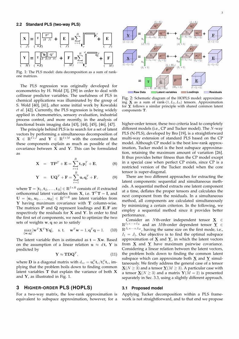
Fig. 1: The PLS model: data decomposition as a sum of rank-one matrices.

The PLS regression was originally developed foreconometrics by H. Wold [3], [39] in order to deal withcollinear predictor variables. The usefulness of PLS inchemical applications was illuminated by the group ofS. Wold [40], [41], after some initial work by Kowalskiet al. [42]. Currently, the PLS regression is being widelyapplied in chemometrics, sensory evaluation, industrialprocess control, and more recently, in the analysis offunctional brain imaging data [43], [44], [45], [46], [47].

The principle behind PLS is to search for a set of latentvectors by performing a simultaneous decomposition ofX ∈ RI×J and Y ∈ RI×M with the constraint thatthese components explain as much as possible of thecovariance between X and Y. This can be formulatedas

X = TPT +E =

R∑r=1

trpTr +E, (8)

Y = UQT + F =

R∑r=1

urqTr + F, (9)

where T = [t1, t2, . . . , tR] ∈ RI×R consists of R extractedorthonormal latent variables from X, i.e. TTT = I, andU = [u1,u2, . . . ,uR] ∈ RI×R are latent variables fromY having maximum covariance with T column-wise.The matrices P and Q represent loadings and E,F arerespectively the residuals for X and Y. In order to findthe first set of components, we need to optimize the twosets of weights w,q so as to satisfy

max{w,q}

[wTXTYq], s. t. wTw = 1,qTq = 1. (10)

The latent variable then is estimated as t = Xw. Basedon the assumption of a linear relation u ≈ d t, Y ispredicted by

Y ≈ TDQT , (11)

where D is a diagonal matrix with drr = uTr tr/t

Tr tr, im-

plying that the problem boils down to finding commonlatent variables T that explain the variance of both Xand Y, as illustrated in Fig. 1.

3 HIGHER-ORDER PLS (HOPLS)For a two-way matrix, the low-rank approximation isequivalent to subspace approximation, however, for a

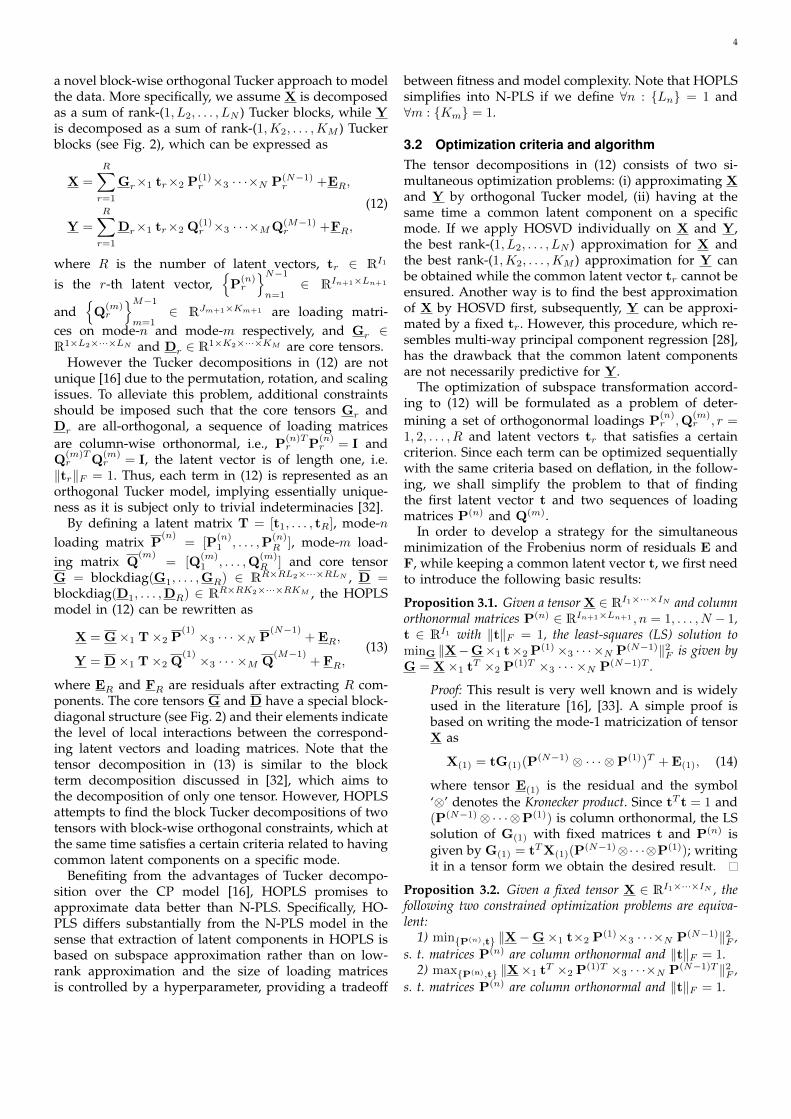
Fig. 2: Schematic diagram of the HOPLS model: approximat-ing X as a sum of rank-(1, L2, L3) tensors. Approximationfor Y follows a similar principle with shared common latentcomponents T.

higher-order tensor, these two criteria lead to completelydifferent models (i.e., CP and Tucker model). The N -wayPLS (N-PLS), developed by Bro [19], is a straightforwardmulti-way extension of standard PLS based on the CPmodel. Although CP model is the best low-rank approx-imation, Tucker model is the best subspace approxima-tion, retaining the maximum amount of variation [26].It thus provides better fitness than the CP model exceptin a special case when perfect CP exists, since CP is arestricted version of the Tucker model when the coretensor is super-diagonal.

There are two different approaches for extracting thelatent components: sequential and simultaneous meth-ods. A sequential method extracts one latent componentat a time, deflates the proper tensors and calculates thenext component from the residuals. In a simultaneousmethod, all components are calculated simultaneouslyby minimizing a certain criterion. In the following, weemploy a sequential method since it provides betterperformance.

Consider an N th-order independent tensor X ∈RI1×···×IN and an M th-order dependent tensor Y ∈RJ1×···×JM , having the same size on the first mode, i.e.,I1 = J1. Our objective is to find the optimal subspaceapproximation of X and Y, in which the latent vectorsfrom X and Y have maximum pairwise covariance.Considering a linear relation between the latent vectors,the problem boils down to finding the common latentsubspace which can approximate both X and Y simul-taneously. We firstly address the general case of a tensorX(N ≥ 3) and a tensor Y(M ≥ 3). A particular case witha tensor X(N ≥ 3) and a matrix Y(M = 2) is presentedseparately in Sec. 3.3, using a slightly different approach.

3.1 Proposed modelApplying Tucker decomposition within a PLS frame-work is not straightforward, and to that end we propose

4

a novel block-wise orthogonal Tucker approach to modelthe data. More specifically, we assume X is decomposedas a sum of rank-(1, L2, . . . , LN ) Tucker blocks, while Yis decomposed as a sum of rank-(1,K2, . . . ,KM ) Tuckerblocks (see Fig. 2), which can be expressed as

X =

R∑r=1

Gr×1 tr×2 P(1)r ×3 · · ·×N P(N−1)

r +ER,

Y =

R∑r=1

Dr×1 tr×2 Q(1)r ×3 · · ·×MQ(M−1)

r +FR,

(12)

where R is the number of latent vectors, tr ∈ RI1

is the r-th latent vector,{P

(n)r

}N−1

n=1∈ RIn+1×Ln+1

and{Q

(m)r

}M−1

m=1∈ RJm+1×Km+1 are loading matri-

ces on mode-n and mode-m respectively, and Gr ∈R1×L2×···×LN and Dr ∈ R1×K2×···×KM are core tensors.

However the Tucker decompositions in (12) are notunique [16] due to the permutation, rotation, and scalingissues. To alleviate this problem, additional constraintsshould be imposed such that the core tensors Gr andDr are all-orthogonal, a sequence of loading matricesare column-wise orthonormal, i.e., P

(n)Tr P

(n)r = I and

Q(m)Tr Q

(m)r = I, the latent vector is of length one, i.e.

‖tr‖F = 1. Thus, each term in (12) is represented as anorthogonal Tucker model, implying essentially unique-ness as it is subject only to trivial indeterminacies [32].

By defining a latent matrix T = [t1, . . . , tR], mode-nloading matrix P

(n)= [P

(n)1 , . . . ,P

(n)R ], mode-m load-

ing matrix Q(m)

= [Q(m)1 , . . . ,Q

(m)R ] and core tensor

G = blockdiag(G1, . . . ,GR) ∈ RR×RL2×···×RLN , D =blockdiag(D1, . . . ,DR) ∈ RR×RK2×···×RKM , the HOPLSmodel in (12) can be rewritten as

X = G×1 T×2 P(1) ×3 · · · ×N P

(N−1)+ER,

Y = D×1 T×2 Q(1) ×3 · · · ×M Q

(M−1)+ FR,

(13)

where ER and FR are residuals after extracting R com-ponents. The core tensors G and D have a special block-diagonal structure (see Fig. 2) and their elements indicatethe level of local interactions between the correspond-ing latent vectors and loading matrices. Note that thetensor decomposition in (13) is similar to the blockterm decomposition discussed in [32], which aims tothe decomposition of only one tensor. However, HOPLSattempts to find the block Tucker decompositions of twotensors with block-wise orthogonal constraints, which atthe same time satisfies a certain criteria related to havingcommon latent components on a specific mode.

Benefiting from the advantages of Tucker decompo-sition over the CP model [16], HOPLS promises toapproximate data better than N-PLS. Specifically, HO-PLS differs substantially from the N-PLS model in thesense that extraction of latent components in HOPLS isbased on subspace approximation rather than on low-rank approximation and the size of loading matricesis controlled by a hyperparameter, providing a tradeoff

between fitness and model complexity. Note that HOPLSsimplifies into N-PLS if we define ∀n : {Ln} = 1 and∀m : {Km} = 1.

3.2 Optimization criteria and algorithmThe tensor decompositions in (12) consists of two si-multaneous optimization problems: (i) approximating Xand Y by orthogonal Tucker model, (ii) having at thesame time a common latent component on a specificmode. If we apply HOSVD individually on X and Y,the best rank-(1, L2, . . . , LN ) approximation for X andthe best rank-(1,K2, . . . ,KM ) approximation for Y canbe obtained while the common latent vector tr cannot beensured. Another way is to find the best approximationof X by HOSVD first, subsequently, Y can be approxi-mated by a fixed tr. However, this procedure, which re-sembles multi-way principal component regression [28],has the drawback that the common latent componentsare not necessarily predictive for Y.

The optimization of subspace transformation accord-ing to (12) will be formulated as a problem of deter-mining a set of orthogonormal loadings P

(n)r ,Q

(m)r , r =

1, 2, . . . , R and latent vectors tr that satisfies a certaincriterion. Since each term can be optimized sequentiallywith the same criteria based on deflation, in the follow-ing, we shall simplify the problem to that of findingthe first latent vector t and two sequences of loadingmatrices P(n) and Q(m).

In order to develop a strategy for the simultaneousminimization of the Frobenius norm of residuals E andF, while keeping a common latent vector t, we first needto introduce the following basic results:

Proposition 3.1. Given a tensor X ∈ RI1×···×IN and columnorthonormal matrices P(n) ∈ RIn+1×Ln+1 , n = 1, . . . , N − 1,t ∈ RI1 with ‖t‖F = 1, the least-squares (LS) solution tominG ‖X−G×1 t×2 P

(1)×3 · · · ×N P(N−1)‖2F is given byG = X×1 t

T ×2 P(1)T ×3 · · · ×N P(N−1)T .

Proof: This result is very well known and is widelyused in the literature [16], [33]. A simple proof isbased on writing the mode-1 matricization of tensorX as

X(1) = tG(1)(P(N−1) ⊗ · · · ⊗P(1))T +E(1), (14)

where tensor E(1) is the residual and the symbol‘⊗’ denotes the Kronecker product. Since tT t = 1 and(P(N−1)⊗ · · ·⊗P(1)) is column orthonormal, the LSsolution of G(1) with fixed matrices t and P(n) isgiven by G(1) = tTX(1)(P

(N−1)⊗· · ·⊗P(1)); writingit in a tensor form we obtain the desired result.

Proposition 3.2. Given a fixed tensor X ∈ RI1×···×IN , thefollowing two constrained optimization problems are equiva-lent:

1) min{P(n),t} ‖X−G×1 t×2 P(1)×3 · · ·×N P(N−1)‖2F ,

s. t. matrices P(n) are column orthonormal and ‖t‖F = 1.2) max{P(n),t} ‖X×1 t

T ×2 P(1)T ×3 · · ·×N P(N−1)T ‖2F ,

s. t. matrices P(n) are column orthonormal and ‖t‖F = 1.

5

The proof is available in [16] (see pp. 477-478).Assume that the orthonormal matrices P(n),Q(m), t

are given, then from Proposition 3.1, the core tensors in(12) can be computed as

G = X×1 tT ×2 P

(1)T ×3 · · ·×N P(N−1)T ,

D = Y ×1 tT ×2 Q

(1)T ×3 · · ·×M Q(M−1)T .(15)

According to Proposition 3.2, minimization of ‖E‖F and‖F‖F under the orthonormality constraint is equivalentto maximization of ‖G‖F and ‖D‖F .

However, taking into account the common latent vec-tor t between X and Y, there is no straightforward wayto maximize ‖G‖F and ‖D‖F simultaneously. To thisend, we propose to maximize a product of norms of twocore tensors, i.e., max{‖G‖2F · ‖D‖2F }. Since the latentvector t is determined by P(n),Q(m), the first step isto optimize the orthonormal loadings, then the commonlatent vectors can be computed by the fixed loadings.

Proposition 3.3. Let G ∈ R1×L2×···×LN and D ∈R1×K2×···×KM , then ‖ < G,D >{1;1} ‖2F = ‖G‖2F · ‖D‖2F .

Proof:

‖ < G,D >{1;1} ‖2F = ‖vec(G)vecT (D)‖2F= trace

(vec(D)vecT (G)vec(G)vecT (D)T

)= ‖vec(G)‖2F · ‖vec(D)‖2F . (16)

where vec(G) ∈ RL2L3...LN is the vectorization ofthe tensor G.

From Proposition 3.3, observe that to maximize‖G‖2F · ‖D‖2F is equivalent to maximizing‖ < G,D >{1;1} ‖2F . According to (15) and tT t = 1,‖ < G,D >{1;1} ‖2F can be expressed as∥∥∥[[< X,Y >{1;1};P

(1)T, . . . ,P(N−1)T ,Q(1)T,. . . ,Q(M−1)T ]]∥∥∥2

F.

(17)Note that this form is quite similar to the optimizationproblem for two-way PLS in (10), where the cross-covariance matrix XTY is replaced by < X,Y >{1;1}.In addition, the optimization item becomes the normof a small tensor in contrast to a scalar in (10). Thus,if we define < X,Y >{1;1} as a mode-1 cross-covariancetensor C = COV{1;1}(X,Y) ∈ RI2×···×IN×J2×···×JM , theoptimization problem can be finally formulated as

max{P(n),Q(m)}

∥∥∥[[C;P(1)T ,. . . ,P(N−1)T ,Q(1)T ,. . .,Q(M−1)T ]]∥∥∥2F

s. t. P(n)TP(n) = ILn+1,Q(m)TQ(m) = IKm+1

, (18)

where P(n), n = 1, . . . , N −1 and Q(m),m = 1, . . . ,M −1are the parameters to optimize.

Based on Proposition 3.2 and orthogonality ofP(n),Q(m), the optimization problem in (18) is equiv-alent to find the best subspace approximation of C as

C ≈ [[G(C);P(1), . . . ,P(N−1),Q(1), . . . ,Q(M−1)]], (19)

which can be obtained by rank-(L2, . . . , LN ,K2, . . . ,KM )HOSVD on tensor C. Based on Proposition 3.1, the

Algorithm 1 The Higher-order Partial Least Squares (HOPLS)Algorithm for a Tensor X and a Tensor Y

Input: X ∈ RI1×···×IN ,Y ∈ RJ1×···×JM , N ≥ 3,M ≥ 3and I1 = J1.Number of latent vectors is R and number of loadingvectors are {Ln}Nn=2 and {Km}Mm=2.

Output: {P(n)r }; {Q(m)

r }; {Gr}; {Dr};Tr = 1, . . . , R; n = 1, . . . , N − 1; m = 1, . . . ,M − 1.Initialization: E1 ← X, F1 ← Y.for r = 1 to R do

if ‖Er‖F > ε and ‖Fr‖F > ε thenCr ←< Er,Fr >{1,1};Rank-(L2, . . . , LN ,K2, . . . ,KM ) orthogonalTucker decomposition of Cr by HOOI [16] asCr ≈ [[G(Cr)

r ;P(1)r , . . . ,P

(N−1)r ,Q

(1)r , . . . ,Q

(M−1)r ]];

tr ← the first leading left singular vector by

SVD[(

Er ×2 P(1)Tr ×3 · · · ×N P

(N−1)Tr

)(1)

];

Gr ← [[Er; tTr ,P

(1)Tr , . . . ,P

(N−1)Tr ]];

Dr ← [[Fr; tTr ,Q

(1)Tr , . . . ,Q

(M−1)Tr ]];

Deflation:Er+1 ← Er − [[Gr; tr,P

(1)r , . . . ,P

(N−1)r ]];

Fr+1 ← Fr − [[Dr; tr,Q(1)r , . . . ,Q

(M−1)r ]];

elseBreak;

end ifend for

optimization term in (18) is equivalent to the normof core tensor G(C). To achieve this goal, the higher-order orthogonal iteration (HOOI) algorithm [16], [37],which is known to converge fast, is employed to findthe parameters P(n) and Q(m) by orthogonal Tuckerdecomposition of C.

Subsequently, based on the estimate of the loadingsP(n) and Q(m), we can now compute the common latentvector t. Note that taking into account the asymmetryproperty of the HOPLS framework, we need to estimatet from predictors X and to estimate regression coefficientD for prediction of responses Y. For a given set of load-ing matrices {P(n)}, the latent vector t should explainvariance of X as much as possible, that is

t = argmint

∥∥∥X− [[G; t,P(1), . . . ,P(N−1)]]∥∥∥2F, (20)

which can be easily achieved by choosing t asthe first leading left singular vector of the matrix(X×2 P

(1)T ×3 · · · ×N P(N−1)T )(1) as used in the HOOIalgorithm (see [16], [35]). Thus, the core tensors G andD are computed by (15).

The above procedure should be carried out repeatedlyusing the deflation operation, until an appropriate num-ber of components (i.e., R) are obtained, or the normsof residuals are smaller than a certain threshold. The

6

deflation1 is performed by subtracting from X and Y theinformation explained by a rank-(1, L2, . . . , LN ) tensor Xand a rank-(1,K2, . . . ,KM ) tensor Y, respectively. TheHOPLS algorithm is outlined in Algorithm 1.

3.3 The case of the tensor X and matrix Y

Suppose that we have an N th-order independent tensorX ∈ RI1×···×IN (N ≥ 3) and a two-way dependent dataY ∈ RI1×M , with the same sample size I1. Since for two-way matrix, subspace approximation is equivalent tolow-rank approximation. HOPLS operates by modelingindependent data X as a sum of rank-(1, L2, . . . , LN )tensors while dependent data Y is modeled with a sumof rank-one matrices as

Y =

R∑r=1

drtrqTr + FR, (21)

where ‖qr‖ = 1 and dr is a scalar.

Proposition 3.4. Let Y ∈ RI×M and q ∈ RM is of lengthone, then t = Yq solves the problem mint ‖Y − tqT ‖2F . Inother words, a linear combination of the columns of Y byusing a weighting vector q of length one has least squaresproperties in terms of approximating Y.

Proof: Since q is given and ‖q‖ = 1, it is obviousthat the ordinary least squares solution to solvethe problem is t = Yq(qTq)−1, hence, t = Yq.If a q with length one is found according to somecriterion, then automatically tqT with t = Yq givesthe best fit of Y for that q.

As discussed in the previous section, the problem ofminimizing ‖E‖2F with respect to matrices P(n) and vec-tor t ∈ RI is equivalent to maximizing the norm of coretensor G with an orthonormality constraint. Meanwhile,we attempt to find an optimal q with unity length whichensures that Yq is linearly correlated with the latentvector t, i.e., dt = Yq, then according to Proposition 3.4,dtqT gives the best fit of Y. Therefore, replacing t byd−1Yq in the expression for the core tensor G in (15),we can optimize the parameters of X-loading matricesP(n) and Y-loading vector q by maximizing the norm ofG, which gives the best approximation of both tensor Xand matrix Y. Finally, the optimization problem of ourinterest can be formulated as:

max{P(n),q}

‖X×1 YT ×1 q

T ×2 P(1)T×3 · · ·×N P(N−1)T ‖2F ,

s. t. P(n)TP(n) = I, ‖q‖F = 1. (22)

where the loadings P(n) and q are parameters to op-timize. This form is similar to (18), but has a differentcross-covariance tensor C = X ×1 Y

T defined betweena tensor and a matrix, implying that the problem can besolved by performing a rank-(1, L2, . . . , LN ) HOSVD on

1. Note that the latent vectors are not orthogonal in HOPLS algo-rithm, which is related to deflation. The theoretical explanation andproof are given in the supplement material.

C. Subsequently, the core tensor G(C) corresponding toC can also be computed.

Next, the latent vector t should be estimated so as tobest approximate X with given loading matrices P(n).According to the model for X, if we take its mode-1matricizacion, we can write

X(1) = tG(1)(P(N−1)T ⊗ · · · ⊗P(1))T +E(1), (23)

where G(1) ∈ R1×L2L3...LN is still unknown. However,the core tensor G (i.e., [[X; tT ,P(1)T , . . . ,P(N−1)T ]]) andthe core tensor G(C) (i.e., [[C;qT ,P(1)T , . . . ,P(N−1)T ]])has a linear connection that G(C) = dG. Therefore,the latent vector t can be estimated in another waythat is different with the previous approach in Section3.2. For fixed matrices G(1) = d−1(G(C))(1), X(1), P(n)

the least square solution for the normalized t, whichminimizes the squared norm of the residual ‖E(1)‖2F , canbe obtained from

t← (X×2P(1)T×3 · · ·×N P(N−1)T )(1)G

(C)+(1) , t← t/‖t‖F ,

(24)where we used the fact that P(n) are columnwise or-thonormal and the symbol ′+′ denotes Moore-Penrosepseudoinverse. With the estimated latent vector t, andloadings q, the regression coefficient used to predict Yis computed as

d = tTYq. (25)

The procedure for a two-way response matrix is sum-marized in Algorithm 2. In this case, HOPLS modelis also shown to unify both standard PLS and N-PLSwithin the same framework, when the appropriate pa-rameters Ln are selected2.

3.4 Prediction of the Response VariablesPredictions from the new observations Xnew are per-formed in two steps: projecting the data to the low-dimensional latent space based on model parametersGr, P

(n)r , and predicting the response data based on

latent vectors Tnew and model parameters Q(m)r , Dr.

For simplicity, we use a matricized form to express theprediction procedure as

Ynew

(1) ≈ TnewQ∗T = Xnew(1) WQ∗T , (26)

where W and Q∗ have R columns, represented by

wr =(P(N−1)

r ⊗ · · · ⊗P(1)r

)G+

r(1),

q∗r = Dr(1)

(Q(M−1)

r ⊗ · · · ⊗Q(1)r

)T.

(27)

In the particular case of a two-way matrix Y, the pre-diction is performed by

Ynew ≈ Xnew(1) WDQT , (28)

where D is a diagonal matrix whose entries are dr andrth column of Q is qr, r = 1, . . . , R.

2. Explanation and proof are given in the supplement material.

7

Algorithm 2 Higher-order Partial Least Squares (HOPLS2)for a Tensor X and a Matrix Y

Input: X ∈ RI1×I2×···×IN , N ≥ 3 and Y ∈ RI1×M

The Number of latent vectors is R and the number ofloadings are {Ln}Nn=2.

Output: {P(n)r };Q; {Gr};D;T; r = 1, . . . , R, n = 2, . . . , N .

Initialization: E1 ← X,F1 ← Y.for r = 1 to R do

if ‖Er‖F > ε and ‖Fr‖F > ε thenCr ← Er ×1 F

Tr ;

Perform rank-(1, L2, · · · , LN ) HOOI on Cr asCr ≈ G(C)

r ×1 qr ×2 P(1)r ×3 · · · ×N P

(N−1)r ;

tr ←(Er ×2 P

(1)r ×3· · ·×N P

(N−1)r

)(1)

(vecT (G(C)

r ))+

;

tr ← tr/‖tr‖F ;Gr ← [[Er; t

Tr ,P

(1)Tr , . . . ,P

(N−1)Tr ]];

ur ← Frqr;dr ← uT

r tr;Deflation:Er+1 ← Er − [[Gr; tr,P

(1)r , . . . ,P

(N−1)r ]];

Fr+1 ← Fr − drtrqTr ;

end ifend for

3.5 Properties of HOPLS

Robustness to noise. An additional constraint of keepingthe largest {Ln}Nn=2 loading vectors on each mode isimposed in HOPLS, resulting in a flexible model thatbalances the two objectives of fitness and the significanceof associated latent variables. For instance, a larger Ln

may fit X better but introduces more noise to eachlatent vector. In contrast, N-PLS is more robust due tothe strong constraint of rank-one tensor structure, whilelacking good fit to the data. The flexibility of HOPLSallows us to adapt the model complexity based onthe dataset in hands, providing considerable predictionability (see Fig. 4, 6).

“Large p, Small n” problem. This is particularly impor-tant when the dimension of independent variables ishigh. In contrast to PLS, the relative low dimension ofmodel parameters that need to be optimized in HOPLS.For instance, assume that a 3th-order tensor X has thedimension of 5 × 10 × 100, i.e., there are 5 samples and1000 features. If we apply PLS on X(1) with size of5×1000, there are only five samples available to optimizea 1000-dimensional loading vector p, resulting in anunreliable estimate of model parameters. In contrast,HOPLS allows us to optimize loading vectors, havingrelatively low-dimension, on each mode alternately; thusthe number of samples is significantly elevated. Forinstance, to optimize 10-dimensional loading vectors onthe second mode, 500 samples are available, and to op-timize the 100-dimensional loading vectors on the thirdmode there are 50 samples. Thus, a more robust estimateof low-dimensional loading vectors can be obtained,

which is also less prone to overfitting and more suitablefor “Large p, Small n” problem (see Fig. 4).

Ease of interpretation. The loading vectors in P(n) revealnew subspace patterns corresponding to the n-modefeatures. However, the loadings from Unfold-PLS are dif-ficult to interpret since the data structure is destroyed bythe unfolding operation and the dimension of loadingsis relatively high.

Computation. N-PLS is implemented by combining aNIPALS-like algorithm with the CP decomposition. In-stead of using an iterative algorithm, HOPLS can findthe model parameters using a closed-form solution, i.e.,applying HOSVD on the cross-covariance tensor, result-ing in enhanced computational efficiency.

Due to the flexibility of HOPLS, the tuning parametersof Ln and Km, controlling the model complexity, needto be selected based on calibration data. Similarly to theparameter R, the tuning parameters can be chosen bycross-validation. For simplicity, two alternative assump-tions will been utilized: a) ∀n, ∀m,Ln = Km = λ; b)Ln = ηRn,Km = ηRm, 0 < η 6 1, i.e., explaining thesame percentage of the n-mode variance.

4 EXPERIMENTAL RESULTS

In the simulations, HOPLS and N-PLS were used tomodel the data in a tensor form whereas PLS was per-formed on a mode-1 matricization of the same tensors.To quantify the predictability, the index Q2 was definedas Q2 = 1 − ‖Y − Y‖2F /‖Y‖2F , where Y denotes theprediction of Y using a model created from a calibrationdataset. Root mean square errors of prediction (RMSEP)were also used for evaluation [48].

4.1 Synthetic dataIn order to quantitatively benchmark our algorithmagainst the state of the art, an extensive comparativeexploration has been performed on synthetic datasets toevaluate the prediction performance under varying con-ditions with respect to data structure, noise levels andratio of variable dimension to sample size. For parameterselection, the number of latent vectors (R) and numberof loadings (Ln = Km = λ) were chosen based on five-fold cross-validation on the calibration dataset. To reducerandom fluctuations, evaluations were performed over50 validation datasets generated repeatedly according tothe same criteria.

4.1.1 Datasets with matrix structureThe independent data X and dependent data Y weregenerated as:

X = TPT + ξE, Y = TQT + ξF, (29)

where latent variables {t,p,q} ∼ N (0, 1), E, F are Gaus-sian noises whose level is controlled by the parameterξ. Both the calibration and the validation datasets weregenerated according to (29), with the same loadings

8

P,Q, but a different latent T which follows the samedistribution N (0, 1). Subsequently, the datasets were re-organized as N th-order tensors.

To investigate how the prediction performance is af-fected by noise levels and small sample size, {X,Y} ∈R20×10×10 (Case 1) and {X,Y} ∈ R10×10×10 (Case 2)were generated under varying noise levels of 10dB, 5dB,0dB and -5dB. In the case 3, {X,Y} ∈ R10×10×10 weregenerated with the loadings P,Q drawn from a uniformdistribution U(0, 1). The datasets were generated fromfive latent variables (i.e., T has five columns) for all thethree cases.

0.1

0.1

0.2

0.2

0.3

0.3

0.4

0.4

0.5

0.5

0.6

10dB

Number of latent variables (R)

Num

ber

of lo

adin

gs (

λ)

2 4 6 8 101

2

3

4

5

6

7

0.05

0.1

0.1

0.15

0.15

0.2

0.2

0.25

0.25

0.3

0.3

0.35

0.35

0.4 0.45

0.45

5dB

Number of latent variables (R)

Num

ber

of lo

adin

gs (

λ)

2 4 6 8 101

2

3

4

5

6

0.060.08

0.1

0.1

0.10.12

0.12

0.14

0.14

0.16

0.16

0.18

0.18

0.2

0.2

0.2

0dB

Number of latent variables (R)

Num

ber

of lo

adin

gs (

λ)

2 4 6 8 101

2

3

4

5

−0.0

5

−0.04

−0.04

−0.0

4

−0.03

−0.03

−0.0

2

−0.02

−0.02

−0.02

−0.0

1

−0.01 −0.01

−0.01 −0.01

0

0

0

0

0

0.01

0.010.020.02

0.03 0.03

−5dB

Number of latent variables (R)

Num

ber

of lo

adin

gs (

λ)

2 4 6 8 101

2

3

4

5

6

Fig. 3: Five-fold cross-validation performance of HOPLS atdifferent noise levels versus the number of latent variables (R)and loadings (λ). The optimal values for these two parametersare marked by green squares.

TABLE 1: The selection of parameters R and λ in Case 2.

SNR PLS N-PLSHOPLS

SNR PLS N-PLSHOPLS

R λ R λ

10dB 5 7 9 6 0dB 3 5 5 45dB 5 6 7 5 -5dB 3 1 3 5

There are two tuning parameters, i.e., number of latentvariables R and number of loadings λ for HOPLS andonly one parameter R for PLS and N-PLS, that need to beselected appropriately. The number of latent variables Ris crucial to prediction performance, resulting in under-modelling when R was too small while overfitting easilywhen R was too large. The cross-validations were per-formed when R and λ were varying from 1 to 10 withthe step length of 1. In order to alleviate the computationburden, the procedure was stopped when the perfor-mance starts to decrease with increasing λ. Fig. 3 showsthe grid of cross-validation performance of HOPLS inCase 2 with the optimal parameters marked by greensquares. Observe that the optimal λ for HOPLS is relatedto the noise levels, and for increasing noise levels, the

best performance is obtained by smaller λ, implying thatonly few significant loadings on each mode are kept inthe latent space. This is expected, due to the fact that themodel complexity is controlled by λ to suppress noise.The optimal R and λ for all three methods at differentnoise levels are shown in Table 1.

Case 1 Case 2 Case 30

0.20.40.60.8

Pre

dict

ed Q

2

SNR=10dB

HOPLS N−PLS PLS

Case 1 Case 2 Case 30

0.2

0.4

0.6

Pre

dict

ed Q

2

SNR=5dB

Case 1 Case 2 Case 30

0.2

0.4P

redi

cted

Q2

SNR=0dB

Case 1 Case 2 Case 30

0.1

0.2

Pre

dict

ed Q

2

SNR=−5dB

Fig. 4: The prediction performance comparison among HO-PLS, N-PLS and PLS at different noise levels for three cases.Case1: {X,Y} ∈ R20×10×10 and {P,Q} ∼ N (0, 1); Case 2:{X,Y} ∈ R10×10×10 and {P,Q} ∼ N (0, 1); Case 3: {X,Y} ∈R10×10×10 and {P,Q} ∼ U(0, 1).

After the selection the parameters, HOPLS, N-PLS andPLS are re-trained on the whole calibration dataset usingthe optimal R and λ, and were applied to the validationdatasets for evaluation. Fig. 4 illustrates the predictiveperformance over 50 validation datasets for the threecases at four different noise levels. In Case 1, a relativelylarger sample size was available, when SNR=10dB, HO-PLS achieved a similar prediction performance to PLSwhile outperforming N-PLS. With increasing the noiselevel in both the calibration and validation datasets,HOPLS showed a relatively stable performance whereasthe performance of PLS decreased significantly. The su-periority of HOPLS was shown clearly with increasingthe noise level. In Case 2 where a smaller sample sizewas available, HOPLS exhibited better performance thanthe other two models and the superiority of HOPLSwas more pronounced at high noise levels, especiallyfor SNR≤5dB. These results demonstrated that HOPLSis more robust to noise in comparison with N-PLS andPLS. If we compare Case 1 with Case 2 at different

9

noise levels, the results revealed that the superiority ofHOPLS over the other two methods was enhanced inCase 2, illustrating the advantage of HOPLS in modelingdatasets with small sample size. Note that N-PLS alsoshowed better performance than PLS when SNR≤0dB inCase 2, demonstrating the advantages of modeling thedataset in a tensor form for small sample sizes. In Case3, N-PLS showed much better performance as comparedto its performance in Case 1 and Case 2, implying sensi-tivity of N-PLS to data distribution. With the increasingnoise level, both HOPLS and N-PLS showed enhancedpredictive abilities over PLS.

4.1.2 Datasets with tensor structureNote that the datasets generated by (29) do not origi-nally possess multi-way data structures although theywere organized in a tensor form, thus the structureinformation of data was not important for prediction.We here assume that HOPLS is more suitable for thedatasets which originally have multi-way structure, i.e.information carried by interaction among each mode areuseful for our regression problem. In order to verifyour assumption, the independent data X and dependentdata Y were generated according to the Tucker modelthat is regarded as a general model for tensors. The latentvariables t were generated in the same way as describedin Section 4.1.1. A sequence of loadings P(n),Q(m) andthe core tensors were drawn from N (0, 1). For the vali-dation dataset, the latent matrix T was generated fromthe same distribution as the calibration dataset, whilethe core tensors and loadings were fixed. Similarly to thestudy in Section 4.1.1, to investigate how the predictionperformance is affected by noise levels and sample size,{X,Y} ∈ R20×10×10 (Case 1) and {X,Y} ∈ R10×10×10

(Case 2) were generated under noise levels of 10dB, 5dB,0dB and -5dB. The datasets for both cases were generatedfrom five latent variables.

TABLE 2: The selection of parameters R and λ in Case 2.

SNR PLS N-PLSHOPLS

SNR PLS N-PLSHOPLS

R λ R λ

10dB 5 7 9 4 0dB 4 4 4 25dB 4 6 8 2 -5dB 2 4 2 1

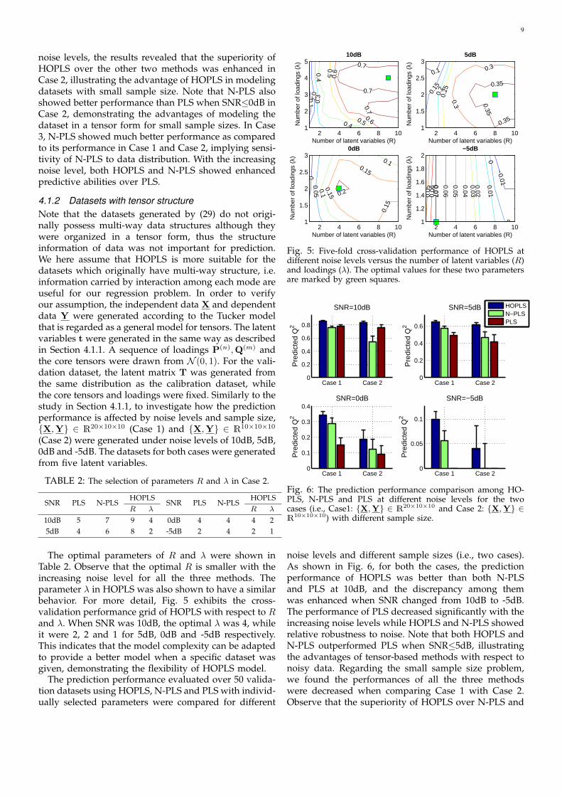
The optimal parameters of R and λ were shown inTable 2. Observe that the optimal R is smaller with theincreasing noise level for all the three methods. Theparameter λ in HOPLS was also shown to have a similarbehavior. For more detail, Fig. 5 exhibits the cross-validation performance grid of HOPLS with respect to Rand λ. When SNR was 10dB, the optimal λ was 4, whileit were 2, 2 and 1 for 5dB, 0dB and -5dB respectively.This indicates that the model complexity can be adaptedto provide a better model when a specific dataset wasgiven, demonstrating the flexibility of HOPLS model.

The prediction performance evaluated over 50 valida-tion datasets using HOPLS, N-PLS and PLS with individ-ually selected parameters were compared for different

0.10.2

0.3

0.4

0.4

0.5

0.5

0.6

0.6

0.7

0.7

0.7

10dB

Number of latent variables (R)

Num

ber

of lo

adin

gs (

λ)

2 4 6 8 101

2

3

4

5

0.1

0.15

0.2

0.25

0.3

0.3

0.35

0.35

0.35

5dB

Number of latent variables (R)

Num

ber

of lo

adin

gs (

λ)

2 4 6 8 101

1.5

2

2.5

3

0

0.050.1

0.1

0.15

0.15

0.15

0.2

0dB

Number of latent variables (R)

Num

ber

of lo

adin

gs (

λ)

2 4 6 8 101

1.5

2

2.5

3

−0.01

0

0

0.01

0.020.030.04

0.05

0.050.06

0.06

0.070.07

−5dB

Number of latent variables (R)

Num

ber

of lo

adin

gs (

λ)

2 4 6 8 101

1.2

1.4

1.6

1.8

2

Fig. 5: Five-fold cross-validation performance of HOPLS atdifferent noise levels versus the number of latent variables (R)and loadings (λ). The optimal values for these two parametersare marked by green squares.

Case 1 Case 20

0.2

0.4

0.6

0.8

Pre

dict

ed Q

2

SNR=10dB

Case 1 Case 20

0.2

0.4

0.6

Pre

dict

ed Q

2

SNR=5dB

HOPLSN−PLSPLS

Case 1 Case 20

0.1

0.2

0.3

0.4

Pre

dict

ed Q

2

SNR=0dB

Case 1 Case 20

0.05

0.1

Pre

dict

ed Q

2SNR=−5dB

Fig. 6: The prediction performance comparison among HO-PLS, N-PLS and PLS at different noise levels for the twocases (i.e., Case1: {X,Y} ∈ R20×10×10 and Case 2: {X,Y} ∈R10×10×10) with different sample size.

noise levels and different sample sizes (i.e., two cases).As shown in Fig. 6, for both the cases, the predictionperformance of HOPLS was better than both N-PLSand PLS at 10dB, and the discrepancy among themwas enhanced when SNR changed from 10dB to -5dB.The performance of PLS decreased significantly with theincreasing noise levels while HOPLS and N-PLS showedrelative robustness to noise. Note that both HOPLS andN-PLS outperformed PLS when SNR≤5dB, illustratingthe advantages of tensor-based methods with respect tonoisy data. Regarding the small sample size problem,we found the performances of all the three methodswere decreased when comparing Case 1 with Case 2.Observe that the superiority of HOPLS over N-PLS and

10

PLS were enhanced in Case 2 as compared to Case 1at all noise levels. A comparison of Fig. 6 and Fig. 4shows that the performances are significantly improvedwhen handling the datasets having tensor structure bytensor-based methods (e.g., HOPLS and N-PLS). As forN-PLS, it outperformed PLS when the datasets havetensor structure and in the presence of high noise, but itmay not perform well when the datasets have no tensorstructure. By contrast, HOPLS performed well in bothcases, in particular, it outperformed both N-PLS and PLSin critical cases with high noise and small sample size.

4.1.3 Comparison on matrix response dataIn this simulation, the response data was a two-waymatrix, thus HOPLS2 algorithm was used to evaluatethe performance. X ∈ R5×5×5×5 and Y ∈ R5×2 weregenerated from a full-rank normal distribution N (0, 1),which satisfies Y = X(1)W where W was also generatedfrom N (0, 1). Fig. 7(A) visualizes the predicted and orig-inal data with the red line indicating the ideal prediction.Observe that HOPLS was able to predict the validationdataset with smaller error than PLS and N-PLS. Theindependent data and dependent data are visualized inthe latent space as shown in Fig. 7(B).

Fig. 7: (A) The scatter plot of predicted against actual datafor each model. (B) Data distribution in the latent vectorspaces. Each blue point denotes one sample of the independentvariable, while the red points denote samples of responsevariables. (C) depicts the distribution of the square error ofprediction on the validation dataset.

4.2 Decoding of ECoG signals

In [46], ECoG-based decoding of 3D hand trajectorieswas demonstrated by means of classical PLS regression3

[49]. The movement of monkeys was captured by anoptical motion capture system (Vicon Motion Systems,USA). In all experiments, each monkey wore a custom-made jacket with reflective markers for motion capture

3. The datasets and more detailed description are freely availablefrom http://neurotycho.org.

affixed to the left shoulder, elbows, wrists and hand,thus the response data was naturally represented as a3th-order tensor (i.e., time × 3D positions × markers).Although PLS can be applied to predict the trajectoriescorresponding to each marker individually, the structureinformation among four markers would be unused. TheECoG data is usually transformed to the time-frequencydomain in order to extract the discriminative features fordecoding movement trajectories. Hence, the independentdata is also naturally represented as a higher-ordertensor (i.e., channel × time × frequency × samples).In this study, the proposed HOPLS regression modelwas applied for decoding movement trajectories basedon ECoG signals to verify its effectiveness in real-worldapplications.

Fig. 8: The scheme for decoding of 3D hand movementtrajectories from ECoG signals.

The overall scheme of ECoG decoding is illustrated inFig. 8. Specifically, ECoG signals were preprocessed by aband-pass filter with cutoff frequencies at 0.1 and 600Hzand a spatial filter with a common average reference.Motion marker positions were down-sampled to 20Hz.In order to represent features related to the movementtrajectory from ECoG signals, the Morlet wavelet trans-formation at 10 different center frequencies (10-150Hz,arranged in a logarithmic scale) was used to obtain thetime-frequency representation. For each sample point of3D trajectories, the most recent one-second ECoG signalswere used to construct predictors. Finally, a three-ordertensor of ECoG features X ∈ RI1×32×100 (samples ×channels × time-frequency) was formed to representindependent data.

We first applied the HOPLS2 algorithm to predict onlythe hand movement trajectory, represented as a matrixY, for comparison with other methods. The ECoG datawas divided into a calibration dataset (10 minutes) anda validation dataset (5 minutes). To select the optimalparameters of Ln and R, the cross-validation was ap-plied on the calibration dataset. Finally, Ln = 10 andR = 23 were selected for the HOPLS model. Likewise,the best values of R for PLS and N-PLS were 19 and60, respectively. The X-latent space is visualized in Fig.9(A), where each point represents one sample of inde-pendent variables, while the Y-latent space is presentedin Fig. 9(B), with each point representing one dependentsample. Observe that the distributions of these two latentvariable spaces were quite similar, and the two dominantclusters are clearly distinguished. The joint distributionsbetween each tr and ur are depicted in Fig. 9(C). Two

11

Fig. 9: Panels (A) and (B) depict data distributions in the X-latent space T and Y-latent space U, respectively. (C) presentsa joint distribution between X- and Y-latent vectors.

clusters can be observed from the first component whichmight be related to the ‘movement’ and ‘non-movement’behaviors.

Fig. 10: (A) Spatial loadings P(1)r corresponding to the first

two latent components. Each row shows 5 significant loadingvectors. Likewise, (B) depicts time-frequency loadings P

(2)r ,

with β and γ-band exhibiting significant contribution.

Another advantage of HOPLS was better physical in-terpretation of the model. To investigate how the spatial,spectral, and temporal structure of ECoG data wereused to create the regression model, loading vectors canbe regarded as a subspace basis in spatial and time-frequency domains, as shown in Fig. 10. With regardto time-frequency loadings, the β- and γ-band activitieswere most significant implying the importance of β, γ-band activities for encoding of movements; the durationof β-band was longer than that of γ-band, which indi-cates that hand movements were related to long historyoscillations of β-band and short history oscillations ofγ-band. These findings also demonstrated that a high

gamma band activity in the premotor cortex is associatedwith movement preparation, initiation and maintenance[50].

From Table 3, observe that the improved predictionperformances were achieved by HOPLS, for all the per-formance metrics. In particular, the results from dataset 1demonstrated that the improvements by HOPLS over N-PLS were 0.03 for the correlation coefficient of X-position,0.02 for averaged RMSEP, 0.04 for averaged Q2, whereasthe improvements by HOPLS over PLS were 0.03 forthe correlation coefficient of X-position, 0.02 for averagedRMSEP, and 0.03 for averaged Q2.

Since HOPLS enables us to create a regressionmodel between two higher-order tensors, all trajecto-ries recorded from shoulder, elbow, wrist and handwere contructed as a tensor Y ∈ RI1×3×4 (samples×3Dpositions×markers). In order to verify the superiorityof HOPLS for small sample sizes, we used 100 seconddata for calibration and 100 second data for validation.The resolution of time-frequency representations was im-proved to provide more detailed features, thus we have a4th-order tensor X ∈ RI1×32×20×20 (samples×channels×time × frequency). The prediction performances fromHOPLS, N-PLS and PLS are shown in Fig. 11, illustratingthe effectiveness of HOPLS when the response dataoriginally has tensor structure.

PLS NPLS HOPLS−0.4

−0.2

0

0.2

0.4

Shoulder

Pre

dict

ion

Q2

PLS NPLS HOPLS−0.4−0.2

00.20.40.60.8

Elbow

PLS NPLS HOPLS0

0.2

0.4

0.6

0.8

1

Wrist

Pre

dict

ion

Q2

PLS NPLS HOPLS0

0.2

0.4

0.6

0.8

1

Hand

X−position Y−position Z−position

Fig. 11: The prediction performance of 3D trajectories recordedfrom shoulder, elbow, wrist and hand. The optimal R are 16,28, 49 for PLS, N-PLS and HOPLS, respectively, and λ = 5 forHOPLS.

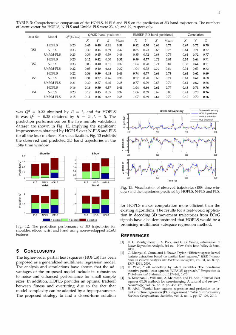
Time-frequency features of the most recent one-secondwindow for each sample are extremely overlapped, re-sulting in a lot of information redundancy and high com-putational burden. In addition, it is generally not neces-sary to predict behaviors with a high time-resolution.Hence, an additional analysis has been performed bydown-sampling motion marker positions at 1Hz, to en-sure that non-overlapped features were used in anyadjacent samples. The cross-validation performance wasevaluated for all the markers from the ten minute cal-ibration dataset and the best performance for PLS ofQ2 = 0.19 was obtained using R = 2, for N-PLS it

12

TABLE 3: Comprehensive comparison of the HOPLS, N-PLS and PLS on the prediction of 3D hand trajectories. The numbersof latent vector for HOPLS, N-PLS and Unfold-PLS were 23, 60, and 19, respectively.

Data Set Model Q2(ECoG)Q2(3D hand positions) RMSEP (3D hand positions) Correlation

X Y Z Mean X Y Z Mean X Y Z

DS1HOPLS 0.25 0.43 0.48 0.61 0.51 0.82 0.70 0.66 0.73 0.67 0.72 0.78N-PLS 0.33 0.39 0.44 0.59 0.47 0.85 0.73 0.68 0.75 0.64 0.71 0.77

Unfold-PLS 0.23 0.39 0.45 0.59 0.48 0.85 0.72 0.68 0.75 0.64 0.72 0.77

DS2HOPLS 0.25 0.12 0.42 0.50 0.35 0.99 0.77 0.72 0.83 0.35 0.64 0.71N-PLS 0.33 0.03 0.40 0.51 0.32 1.04 0.78 0.71 0.84 0.32 0.64 0.71

Unfold-PLS 0.22 0.05 0.40 0.53 0.32 1.04 0.78 0.70 0.84 0.34 0.63 0.73

DS3HOPLS 0.22 0.36 0.39 0.48 0.41 0.74 0.77 0.66 0.73 0.62 0.62 0.69N-PLS 0.30 0.31 0.37 0.46 0.38 0.77 0.78 0.68 0.74 0.61 0.62 0.68

Unfold-PLS 0.21 0.30 0.37 0.46 0.38 0.77 0.79 0.67 0.74 0.61 0.62 0.68

DS4HOPLS 0.16 0.16 0.50 0.57 0.41 1.04 0.66 0.62 0.77 0.43 0.71 0.76N-PLS 0.23 0.12 0.45 0.55 0.37 1.06 0.69 0.67 0.80 0.41 0.70 0.76

Unfold-PLS 0.15 0.11 0.46 0.57 0.38 1.07 0.69 0.62 0.79 0.42 0.70 0.76

was Q2 = 0.22 obtained by R = 5, and for HOPLSit was Q2 = 0.28 obtained by R = 24, λ = 5. Theprediction performances on the five minute validationdataset are shown in Fig. 12, implying the significantimprovements obtained by HOPLS over N-PLS and PLSfor all the four markers. For visualization, Fig. 13 exhibitsthe observed and predicted 3D hand trajectories in the150s time window.

PLS NPLS HOPLS

0

0.2

0.4

0.6

0.8Shoulder

Pre

dict

ion

Q2

PLS NPLS HOPLS

0

0.2

0.4

0.6

0.8

1

Elbow

PLS NPLS HOPLS0

0.5

1

Wrist

Pre

dict

ion

Q2

PLS NPLS HOPLS0

0.5

1

Hand

X−position Y−position Z−position

Fig. 12: The prediction performance of 3D trajectories forshoulder, elbow, wrist and hand using non-overlapped ECoGfeatures.

5 CONCLUSIONS

The higher-order partial least squares (HOPLS) has beenproposed as a generalized multilinear regression model.The analysis and simulations have shown that the ad-vantages of the proposed model include its robustnessto noise and enhanced performance for small samplesizes. In addition, HOPLS provides an optimal tradeoffbetween fitness and overfitting due to the fact thatmodel complexity can be adapted by a hyperparameter.The proposed strategy to find a closed-form solution

150 200 250 300

0

2

4

63D hand trajectory

X−

posi

tion

150 200 250 300

−3−2−1

01

Y−

posi

tion

150 200 250 300

−1

0

1

2

3

Z−

posi

tion

Time (s)

Observed trajectoryHOPLS predictionN−PLS predictionPLS prediction

Fig. 13: Visualization of observed trajectories (150s time win-dow) and the trajectories predicted by HOPLS, N-PLS and PLS.

for HOPLS makes computation more efficient than theexisting algorithms. The results for a real-world applica-tion in decoding 3D movement trajectories from ECoGsignals have also demonstrated that HOPLS would be apromising multilinear subspace regression method.

REFERENCES

[1] D. C. Montgomery, E. A. Peck, and G. G. Vining, Introduction toLinear Regression Analysis, 3rd ed. New York: John Wiley & Sons,2001.

[2] C. Dhanjal, S. Gunn, and J. Shawe-Taylor, “Efficient sparse kernelfeature extraction based on partial least squares,” IEEE Transac-tions on Pattern Analysis and Machine Intelligence, vol. 31, no. 8, pp.1347–1361, 2009.

[3] H. Wold, “Soft modelling by latent variables: The non-lineariterative partial least squares (NIPALS) approach,” Perspectives inProbability and Statistics, pp. 117–142, 1975.

[4] A. Krishnan, L. Williams, A. McIntosh, and H. Abdi, “Partial leastsquares (PLS) methods for neuroimaging: A tutorial and review,”NeuroImage, vol. 56, no. 2, pp. 455–475, 2010.

[5] H. Abdi, “Partial least squares regression and projection on la-tent structure regression (PLS Regression),” Wiley InterdisciplinaryReviews: Computational Statistics, vol. 2, no. 1, pp. 97–106, 2010.

13

[6] R. Rosipal and N. Kramer, “Overview and recent advances in par-tial least squares,” Subspace, Latent Structure and Feature Selection,pp. 34–51, 2006.

[7] J. Trygg and S. Wold, “Orthogonal projections to latent structures(O-PLS),” Journal of Chemometrics, vol. 16, no. 3, pp. 119–128, 2002.

[8] R. Ergon, “PLS score-loading correspondence and a bi-orthogonalfactorization,” Journal of Chemometrics, vol. 16, no. 7, pp. 368–373,2002.

[9] S. Vijayakumar and S. Schaal, “Locally weighted projection regres-sion: An O (n) algorithm for incremental real time learning in highdimensional space,” in Proceedings of the Seventeenth InternationalConference on Machine Learning, vol. 1, 2000, pp. 288–293.

[10] R. Rosipal and L. Trejo, “Kernel partial least squares regression inreproducing kernel Hilbert space,” The Journal of Machine LearningResearch, vol. 2, p. 123, 2002.

[11] J. Ham, D. Lee, S. Mika, and B. Scholkopf, “A kernel view ofthe dimensionality reduction of manifolds,” in Proceedings of thetwenty-first international conference on Machine learning. ACM,2004, pp. 47–54.

[12] R. Bro, A. Rinnan, and N. Faber, “Standard error of prediction formultilinear PLS-2. Practical implementation in fluorescence spec-troscopy,” Chemometrics and Intelligent Laboratory Systems, vol. 75,no. 1, pp. 69–76, 2005.

[13] B. Li, J. Morris, and E. Martin, “Model selection for partialleast squares regression,” Chemometrics and Intelligent LaboratorySystems, vol. 64, no. 1, pp. 79–89, 2002.

[14] R. Tibshirani, “Regression shrinkage and selection via the lasso,”Journal of the Royal Statistical Society. Series B (Methodological), pp.267–288, 1996.

[15] R. Bro, “Multi-way analysis in the food industry,” Models, Algo-rithms, and Applications. Academish proefschrift. Dinamarca, 1998.

[16] T. Kolda and B. Bader, “Tensor Decompositions and Applica-tions,” SIAM Review, vol. 51, no. 3, pp. 455–500, 2009.

[17] A. Cichocki, R. Zdunek, A. H. Phan, and S. I. Amari, NonnegativeMatrix and Tensor Factorizations. John Wiley & Sons, 2009.

[18] E. Acar, D. Dunlavy, T. Kolda, and M. Mørup, “Scalable tensorfactorizations for incomplete data,” Chemometrics and IntelligentLaboratory Systems, 2010.

[19] R. Bro, “Multiway calibration. Multilinear PLS,” Journal of Chemo-metrics, vol. 10, no. 1, pp. 47–61, 1996.

[20] ——, “Review on multiway analysis in chemistry2000–2005,”Critical Reviews in Analytical Chemistry, vol. 36, no. 3, pp. 279–293,2006.

[21] K. Hasegawa, M. Arakawa, and K. Funatsu, “Rational choice ofbioactive conformations through use of conformation analysis and3-way partial least squares modeling,” Chemometrics and IntelligentLaboratory Systems, vol. 50, no. 2, pp. 253–261, 2000.

[22] J. Nilsson, S. de Jong, and A. Smilde, “Multiway calibration in 3DQSAR,” Journal of chemometrics, vol. 11, no. 6, pp. 511–524, 1997.

[23] K. Zissis, R. Brereton, S. Dunkerley, and R. Escott, “Two-way, un-folded three-way and three-mode partial least squares calibrationof diode array HPLC chromatograms for the quantitation of low-level pharmaceutical impurities,” Analytica Chimica Acta, vol. 384,no. 1, pp. 71–81, 1999.

[24] E. Martinez-Montes, P. Valdes-Sosa, F. Miwakeichi, R. Goldman,and M. Cohen, “Concurrent EEG/fMRI analysis by multiwaypartial least squares,” NeuroImage, vol. 22, no. 3, pp. 1023–1034,2004.

[25] E. Acar, C. Bingol, H. Bingol, R. Bro, and B. Yener, “Seizure recog-nition on epilepsy feature tensor,” in 29th Annual InternationalConference of the IEEE EMBS 2007, 2007, pp. 4273–4276.

[26] R. Bro, A. Smilde, and S. de Jong, “On the difference between low-rank and subspace approximation: improved model for multi-linear PLS regression,” Chemometrics and Intelligent LaboratorySystems, vol. 58, no. 1, pp. 3–13, 2001.

[27] A. Smilde and H. Kiers, “Multiway covariates regression models,”Journal of Chemometrics, vol. 13, no. 1, pp. 31–48, 1999.

[28] A. Smilde, R. Bro, and P. Geladi, Multi-way analysis with applica-tions in the chemical sciences. Wiley, 2004.

[29] R. A. Harshman, “Foundations of the PARAFAC procedure: Mod-els and conditions for an explanatory multimodal factor analysis,”UCLA Working Papers in Phonetics, vol. 16, pp. 1–84, 1970.

[30] A. Smilde, “Comments on multilinear PLS,” Journal of Chemomet-rics, vol. 11, no. 5, pp. 367–377, 1997.

[31] M. D. Borraccetti, P. C. Damiani, and A. C. Olivieri, “Whenunfolding is better: unique success of unfolded partial least-squares regression with residual bilinearization for the processing

of spectral-pH data with strong spectral overlapping. analysisof fluoroquinolones in human urine based on flow-injection pH-modulated synchronous fluorescence data matrices,” Analyst, vol.134, pp. 1682–1691, 2009.

[32] L. De Lathauwer, “Decompositions of a higher-order tensor inblock terms - Part II: Definitions and uniqueness,” SIAM J. MatrixAnal. Appl, vol. 30, no. 3, pp. 1033–1066, 2008.

[33] L. De Lathauwer, B. De Moor, and J. Vandewalle, “A multilinearsingular value decomposition,” SIAM Journal on Matrix Analysisand Applications, vol. 21, no. 4, pp. 1253–1278, 2000.

[34] L. R. Tucker, “Implications of factor analysis of three-way matricesfor measurement of change,” in Problems in Measuring Change,C. W. Harris, Ed. University of Wisconsin Press, 1963, pp. 122–137.

[35] T. Kolda, Multilinear operators for higher-order decompositions. Tech.Report SAND2006-2081, Sandia National Laboratories, Albu-querque, NM, Livermore, CA, 2006.

[36] J. D. Carroll and J. J. Chang, “Analysis of individual differences inmultidimensional scaling via an N-way generalization of “Eckart-Young”decomposition,” Psychometrika, vol. 35, pp. 283–319, 1970.

[37] L. De Lathauwer, B. De Moor, and J. Vandewalle, “On the BestRank-1 and Rank-(R1, R2,..., RN) Approximation of Higher-OrderTensors,” SIAM Journal on Matrix Analysis and Applications, vol. 21,no. 4, pp. 1324–1342, 2000.

[38] L.-H. Lim and V. D. Silva, “Tensor rank and the ill-posednessof the best low-rank approximation problem,” SIAM Journal ofMatrix Analysis and Applications, vol. 30, no. 3, pp. 1084–1127, 2008.

[39] H. Wold, “Soft modeling: the basic design and some extensions,”Systems Under Indirect Observation, vol. 2, pp. 1–53, 1982.

[40] S. Wold, M. Sjostroma, and L. Erikssonb, “PLS-regression: abasic tool of chemometrics,” Chemometrics and Intelligent LaboratorySystems, vol. 58, pp. 109–130, 2001.

[41] S. Wold, A. Ruhe, H. Wold, and W. Dunn III, “The collinearityproblem in linear regression. The partial least squares (PLS)approach to generalized inverses,” SIAM Journal on Scientific andStatistical Computing, vol. 5, p. 735, 1984.

[42] B. Kowalski, R. Gerlach, and H. Wold, “Systems under indirectobservation,” Chemical Systems under Indirect Observation, pp. 191–209, 1982.

[43] A. McIntosh and N. Lobaugh, “Partial least squares analysisof neuroimaging data: applications and advances,” Neuroimage,vol. 23, pp. S250–S263, 2004.

[44] A. McIntosh, W. Chau, and A. Protzner, “Spatiotemporal analysisof event-related fMRI data using partial least squares,” Neuroim-age, vol. 23, no. 2, pp. 764–775, 2004.

[45] N. Kovacevic and A. McIntosh, “Groupwise independent compo-nent decomposition of EEG data and partial least square analy-sis,” NeuroImage, vol. 35, no. 3, pp. 1103–1112, 2007.

[46] Z. Chao, Y. Nagasaka, and N. Fujii, “Long-term asynchronousdecoding of arm motion using electrocorticographic signals inmonkeys,” Frontiers in Neuroengineering, vol. 3, no. 3, 2010.

[47] L. Trejo, R. Rosipal, and B. Matthews, “Brain-computer interfacesfor 1-D and 2-D cursor control: designs using volitional controlof the EEG spectrum or steady-state visual evoked potentials,”IEEE Transactions on Neural Systems and Rehabilitation Engineering,vol. 14, no. 2, pp. 225–229, 2006.

[48] H. Kim, J. Zhou, H. Morse III, and H. Park, “A three-stageframework for gene expression data analysis by L1-norm supportvector regression,” International Journal of Bioinformatics Researchand Applications, vol. 1, no. 1, pp. 51–62, 2005.

[49] Y. Nagasaka, K. Shimoda, and N. Fujii, “Multidimensional record-ing (MDR) and data sharing: An ecological open research andeducational platform for neuroscience,” PLoS ONE, vol. 6, no. 7,p. e22561, 2011.

[50] J. Rickert, S. de Oliveira, E. Vaadia, A. Aertsen, S. Rotter, andC. Mehring, “Encoding of movement direction in different fre-quency ranges of motor cortical local field potentials,” The Journalof Neuroscience, vol. 25, no. 39, pp. 8815–8824, 2005.