Embed Size (px)
Citation preview

Hiring and RetentionIssues in Police Agencies:Readings on theDeterminants of PoliceStrength, Hiring andRetention of Officers, andthe Federal COPS Program
Christopher S. Koper (Principal Investigator)Edward R. MaguireGretchen E. Moorewith contributions by David E. Huffer
Report to the National Institute of JusticeGrant # NIJ 99-IJ-CX-0011
URBAN INSTITUTEJustice Policy Center
research for safer communities
RE
SE
AR
CH
R
EP
OR
TO
ctober 20
01


URBAN INSTITUTEJustice Policy Center2100 M STREET, NWWASHINGTON, DC 20037www.urban.org
The views expressed are those of the authors, and should not beattributed to The Urban Institute, its trustees, or its funders.
Contents
The Authors and Contributors ..........................................................................................................................................................iiAcknowledgements .........................................................................................................................................................................ii
Key Findings at a Glance................................................................................................................... iiiDeterminants of Sworn Force Strength............................................................................................................................................iiiHiring and Training Officers ............................................................................................................................................................iiiOfficer Attrition and Tenure............................................................................................................................................................iiiRetention of COPS-Funded Positions .............................................................................................................................................. iv
CHAPTER 1. Introduction and Summary.............................................................................................11.1. Introduction: Study Background and Scope .................................................................................................11.2. Summary of Findings..................................................................................................................................21.3. Retention of COPS-Funded Positions and Historical Patterns of Staff Retention............................................4
CHAPTER 2. Research Evidence on the Factors Influencing Police Strength in the United States ....................72.1. Introduction................................................................................................................................................72.2. The Evolution of Research on Police Strength..............................................................................................92.3. Discussion and Conclusions ..................................................................................................................... 24
CHAPTER 3. A Survey-Based Assessment of Factors Causing Changesin Sworn Force Size: Examining the Perceptions of Police.................................................. 273.1. Introduction............................................................................................................................................. 273.2. Data and Methods ................................................................................................................................... 283.3. Recent Patterns of Change in the Size of Police Agencies ......................................................................... 313.4. Factors Causing Increases and Decreases in Sworn Force Strength, 1996-1999 ....................................... 313.5. Racial / Economic Conflict and Police Growth .......................................................................................... 353.6. Discussion............................................................................................................................................... 40
CHAPTER 4. Hiring, Training, and Retention of Police Officers:A National Examination of Patterns and Emerging Trends................................................... 414.1. Hiring and Training Officers ..................................................................................................................... 424.2. Officer Attrition and Tenure...................................................................................................................... 464.3. Discussion............................................................................................................................................... 48Appendix 4.A. Officer Allocation and the COPS Program: Some Thoughts aboutFuture Lines of Inquiry ..................................................................................................................................... 50
CHAPTER 5. Retention of Staff Positions Funded through the Federal Cops Program:Comparing Retention Rates among Cops Agencies to Historical Patternsof Staff Retention in Police Agencies .............................................................................. 555.1. Retention of Staffing Increases Funded by COPS Hiring Grants ................................................................. 565.2. Historical Patterns of Staff Retention Following Periods of Agency Growth ................................................ 595.3. Comparing Retention Rates Among COPS Grantees to Historical Retention Patterns.................................. 65
References .............................................................................................................................. 66
Methodological Appendix. The Police Hiring and Retention (H&R) Survey................................................... 70A.1. Overview of the COPS-Police Hiring and Retention Survey Sample........................................................................................ 70A.2. Development of the Sample Design...................................................................................................................................... 71

ii
THE AUTHORS AND CONTRIBUTORS
Christopher S. Koper, Ph.D., Research Associate, Jerry Lee Center of Criminology, University ofPennsylvania.
Edward R. Maguire, Ph.D., Associate Professor, Administration of Justice Program, GeorgeMason University.
Gretchen E. Moore, M.A., Research Associate, The Urban Institute.David E. Huffer, M.A., doctoral student, Department of Criminology and Criminal Justice,
University of Maryland.
ACKNOWLEDGEMENTS
This study was supported by grant 99-IJ-CX-0011 from the National Institute of Justice (U.S.Department of Justice) to the Urban Institute. Additional support was provided by the Jerry LeeCenter of Criminology of the University of Pennsylvania.
The authors wish to thank a number of people and organizations that assisted this project invarious ways. Staff of the National Opinion Research Center (NORC) conducted the telephoneinterviews for the Police Hiring and Retention Survey. Alma Kuby and Laurie Imhoff managedNORC’s efforts in planning and implementing the interviews. They and other NORC staff providedfeedback on the survey instrument. Thanks go to NORC staff for completing the survey on time,under budget, and with high response rates. Thanks also go, of course, to the 1,270 police chiefs andtheir designees who agreed to participate in the survey.
Jeffrey Roth assisted in the development of the survey instrument and lent advice on variousaspects of the project. Michael Buerger, Joseph Ryan, Alberto Melis, and Ray Manus providedhelpful comments on early versions of the survey instrument. Ruth White provided researchassistance in the early stages of the project, and Rob Santos also assisted in the early phases of projectdevelopment. David Williams formatted the draft and final versions of the report and provided otherresearch assistance.
Staff of the federal Office of Community Oriented Policing Services, particularly Rob Chapman,Pam Cammarata, and Veh Bezdikian, helped define several research issues for the study, providedCOPS Office databases, and offered comments on draft versions of the survey instrument and report.At the National Institute of Justice (NIJ), Steve Edwards served as grant monitor, providing advice andmanagerial support. Anonymous reviewers for NIJ gave valuable comments on the draft version ofthe report.
The opinions expressed in the report are those of the authors and should not be attributed to anyof the aforementioned persons or organizations.
iii
Key Findings at a Glance
This report presents a series of papers addressing a number of staffing issues in policing:determinants of police staffing levels; the processes of hiring and training officers; and retentionpatterns associated with individual officers and staff positions. The papers are the result of an UrbanInstitute project funded by the National Institute of Justice to develop baseline data and knowledgethat could prove useful in managing and assessing the federal Community Oriented Policing Services(COPS) program (the federal government’s initiative to put 100,000 additional police on the streetsthrough hiring grants and other means) as well as inform other research and policy issues in policing.
Most findings are based on results from a telephone survey with a nationally representativeprobability sample of 1,270 police agencies. The survey analyses are supplemented by analyses ofnational data on police employment and reviews of prior studies on the determinants of policestrength. We present many findings separately for small jurisdictions (those with populations smallerthan 50,000 persons) and large jurisdictions (those with 50,000 or more persons). Key findings fromthe study include the following.
DETERMINANTS OF SWORN FORCE STRENGTH
Factors influencing police strength (measured in terms of officers or expenditures) are not wellunderstood. A review of 55 empirical studies on the determinants of police strength across placesand/or over time revealed inconsistent findings for variables commonly used to predict police strength.
New survey analyses measuring the perceptions of police suggest that grant money, crime, callsfor service, and population were some of the leading contributors to police growth from 1996 to 1999.Fiscal constraints and the lack of qualified recruits were two of the leading factors associated withpolice decline during this same period. Some factors linked to police staffing may be differentiallyassociated with police growth and decline; most notably, crime may contribute to growth in staffingbut not have much influence on reductions in staffing.
HIRING AND TRAINING OFFICERS
The process of screening and training new officers takes an average of 31 weeks in smallagencies and 43 weeks in large agencies. Ninety-two of every one hundred new hires in smallagencies and eighty-nine of one hundred in large agencies successfully complete all training.
Slightly less than 60% of agencies reported that the length of the training process has increased inrecent years due to new training requirements, some of which involve training for communitypolicing.
Over half of small agencies and two-thirds of large agencies reported that a lack of qualifiedapplicants caused difficulties in filling recent vacancies. Close to half of small agencies and over halfof large agencies also reported modest staffing problems caused by unanticipated vacancies.
OFFICER ATTRITION AND TENURE
Officers serve for shorter periods in small agencies than in large agencies. Half of officersleaving large agencies but only a fifth of those leaving small agencies are retirees. Further, two-thirds

iv
of departing officers in small agencies and about a third of those in large agencies leave after five orless years of service. It is estimated that nearly half of officers departing small agencies and about aquarter of those leaving large agencies go on to other law enforcement work.
RETENTION OF COPS-FUNDED POSITIONS
Based on short-term (1-2 years) follow-up data, approximately three-quarters of agencies withexpired COPS grants have retained their COPS-funded positions (to this point, virtually all retainingagencies have kept all of their COPS positions). About two-thirds of grantees expect to keep all oftheir non-expired COPS positions, while 74% of small grantees and 80% of large grantees expect tokeep at least some of their non-expired COPS positions. Most of these agencies expect to retain theCOPS positions for 5 or more years.
Overall, observed and expected retention rates among COPS grantees appear to be fairlyconsistent with historical retention patterns, based on a national analysis of twenty years of policeemployment data which examined retention of new positions by police organizations followingperiods when the organizations grew substantially.

Introduction and Summary 1
CHAPTER 1.
Introduction and SummaryChristopher S. Koper
1.1. INTRODUCTION: STUDY BACKGROUND AND SCOPE
This report contains a collection of readings that examine various staffing issues in policing.These readings address three broad issues: determinants of police staffing levels; the processes ofhiring, training, and deploying officers; and retention patterns associated with individual officers andstaff positions. The papers are the result of an Urban Institute research project funded by the NationalInstitute of Justice to, in large part, answer questions of interest to policymakers in the Office ofCommunity Oriented Policing Services (i.e., the COPS Office), the agency that administers the federalCommunity Oriented Policing Services program. Passed by Congress as part of the Violent CrimeControl and Law Enforcement Act of 1994, the COPS program is the federal government’s initiative toadd 100,000 officers to the nation’s police agencies through grants for hiring new officers and othermeans (see Roth et al. 2000a for an in-depth description and evaluation of the COPS program).
COPS Office staff sought answers to a number of questions that would assist them in planning,managing, and assessing the COPS program. However, direct evaluation of the COPS program was notthe focus of this research effort. Instead, the project emphasized the development of baseline data andknowledge that could prove useful in managing and evaluating various aspects of the COPS program,such as grantees’ progress in hiring and deploying officers and grantees’ retention of COPS-fundedpositions. Based on discussions with COPS Office staff and additional considerations, we identified aseries of general research questions covering a range of loosely related police staffing issues.
§ What factors determine the size of police agencies, i.e., what factors influence variation inagency size across places and over time? Are these factors similar for large and small policeorganizations? Are the factors contributing to police growth different from those leading toreductions in police?
§ How long does it typically take to hire, train, and deploy police officers? What are theattrition rates in this process? What problems do agencies encounter in hiring and trainingofficers?
§ How long do officers serve with their agencies and under what circumstances do they leave?
§ How long do agencies maintain new positions following periods of growth, irrespective ofthe particular officers filling those positions? How do current and expected retention ratesfor COPS-funded positions compare to historical norms of staff retention?
Though these questions are clearly relevant to the administration and assessment of the COPSprogram, they have broader relevance to several research and policy issues.
In order to address these issues, project staff utilized a number of methods: critical synthesis ofliterature, analysis of secondary data sources, and collection and analysis of survey data. The largestpart of the research effort involved the development of a telephone survey that was administered duringthe summer of 2000 to a nationally representative sample of nearly 1,300 police agencies. The survey,

2 Chapter 1
referred to hereafter as the Police Hiring and Retention (H&R) Survey, is described in theMethodological Appendix. Most of the chapters in this volume are based on analyses of the H&Rsurvey data.
Due to the range of topics explored in this project, the style of this report is more like that of anedited book volume than a report with tightly integrated chapters. The remaining chapters of thereport are divided into two parts. Part I consists of chapters Two and Three which examine thedeterminants of police agency size using, respectively, critical assessment of existing literature andsurvey data analysis. Employing these complementary approaches, these chapters investigate thefactors, many of them external to police agencies, which cause variation in the size of policeorganizations across places and over time.
The determinants of sworn force levels investigated in Chapters Two and Three influencepolicymakers as they establish target levels of policing for their jurisdictions. Once those target levelsof policing are established, however, the processes of hiring, training, and retaining officers affect boththe speed with which agencies can reach these target staffing levels and their ability to maintain them.Hiring and retention issues are the subjects of chapters Four and Five, which constitute Part II of thereport. Using the H&R survey data, Chapter Four provides descriptive analyses of various aspects ofpolice hiring and retention patterns, including the length of time it takes agencies to hire and train newofficers and the length of time that officers serve with their agencies. Finally, employing both theH&R survey data and analysis of national police employment data, Chapter Five examines retentionrates for police positions funded through the COPS program and compares these retention rates tohistorical retention norms in police agencies.
1.2. SUMMARY OF FINDINGS
1.2.1. Determinants of Sworn Force Strength
Scholars have used three theoretical frameworks to explain variation in police strength. Rationalpublic choice theory links variation in police strength to variables such as crime and population, whichreflect demand for police services. Conflict theory holds that governments increase their police forcesin response to growth in populations that dominant groups deem to be threatening. Threateningpopulations may be defined in racial terms (e.g., non-white groups) or in economic terms (e.g., thepoor and unemployed). Finally, organizational theory stresses internal organizational factors thatinfluence the size of police agencies. Empirically, scholars typically approximate these factors byusing yesterday’s police strength to predict today’s police strength.
However, the factors influencing police strength are not well understood. Chapter Two reviews55 empirical studies on the determinants of police strength, revealing that with the exception of theprior (i.e., lagged) size of the police force, none of the factors commonly studied have been shown toinfluence police levels on a consistent basis. Consider, for example, the impact of violent crime onpolice strength. Though one would expect that increases in violent crime lead to police growth, only48% of the studies examining the impact of violent crime on police found the expected positiveassociation. Forty-five percent of the studies found no statistically meaningful effect of violent crimeon police, and seven percent found a significant inverse relationship between these variables(suggesting that increases in violent crime lead to reductions in police strength). The mixed findingsof prior research are largely attributable to a number of methodological points, such as variation in thedefinition of police strength across studies (some studies measure police strength in terms of personnelwhile others measure it in terms of expenditures), variation in the unit of analysis across studies (e.g.,cities, states, etc.), poor and/or inconsistent model specification, and complexities involved indisentangling the mutual effects which variables like crime and police levels have upon each other.

Introduction and Summary 3
Chapter Two concludes with recommendations for improving research in this area. Among theseis the call for more research on the interpretations and assessments of actors who make decisions aboutpolice strength. Indeed, prior studies have generally treated the decision-making process as a blackbox, using aggregate-level correlations between police strength and other factors to make indirectinferences about the process. Chapter Three takes a modest step towards rectifying this by using theH&R survey data to examine police officials’ perceptions about factors that caused changes in the sizeof their agencies from 1996 through 1999. An advantage to studying the determinants of policestrength in this way is that it taps into the perceptions of people who have insight into the actualprocess by which staffing levels are set.
Overall, the study period was characterized by police growth. Slightly over half of policeagencies grew during this period, while only 11% of large agencies (defined as those servingjurisdictions of 50,000 or more persons) and 22% of small agencies (defined as those servingjurisdictions with fewer than 50,000 persons) decreased in size. Respondents’ perceptions supportedsome of the leading theories about influences on police staffing: among both large and small agencies,changes in crime, calls for service, and population had important influences on growing agencies,while changes in government revenue and fiscal constraints (including generally declining economicconditions) had notable impacts on shrinking agencies.
As the preceding statement suggests, however, some of the factors associated with changes inpolice staffing may have differential effects on growth and decline in police agencies. If true, this mayhelp to explain some of the conflicting findings of past research. Most notably, police perceptionssuggest that crime fuels growth in staffing but that it has little or no influence on reductions in staffing.Rather than causing cutbacks in police, perhaps the potential impact of declining crime rates on policestaffing is mitigated by organizational inertia and the political difficulties of reducing police forces.This implies that rising crime rates have more impact on police agencies than do declining crime rates.Consequently, the results of any given study of crime and police staffing could be highly contingenton crime trends during the study period and assumptions about the functional form of the relationshipbetween the variables.
Two additional factors that had strong influences on recent trends in police staffing were grantmoney and the availability of qualified recruits. Police in both growing and shrinking agencies ratedthe availability of grant money as the first or second most important factor affecting changes in thesize of their agencies (for shrinking agencies, the findings suggest that the availability of grant moneyprevented the agencies from declining further and/or that the absence of grant money facilitatedreductions in force). The importance of grant money to both growing and declining agencies suggeststhat the federal COPS program has perhaps been the single most important factor both facilitatinggrowth and slowing reductions in police strength during the latter 1990s, though we should temper thisconclusion by noting that the study did not distinguish between the effects of COPS hiring grants andother federal or state hiring grants available during the study period. The availability of qualifiedrecruits, or the lack thereof, was an important factor cited by respondents in agencies with decliningstaff, a finding echoed elsewhere in the report. This finding would seem to be linked to the strongeconomy of recent years; ironically, strong economic times may boost funds available for policing butmake it more difficult for police organizations to attract and retain recruits.
1.2.2. Hiring, Training, and Retention of Officers
As noted above, police staffing levels are also affected by the success of agencies in hiring,training, and retaining officers. The H&R survey provided a descriptive snapshot of hiring andretention patterns in police organizations as of the summer of 2000.
The process of screening and training new officers takes an average of 31 weeks in smallagencies and 43 weeks in large agencies. Ninety-two of every one hundred new hires in smallagencies and eighty-nine of every one-hundred new hires in large agencies complete all trainingsuccessfully. Nearly 60% of agencies reported that their training time had increased in recent years
4 Chapter 1
(only 4% reported a decrease in the length of training). Among agencies reporting an increase intraining time, about a third reported that new training requirements associated with communitypolicing had contributed to the increase.
Over half of small agencies and two-thirds of large agencies reported that a lack of qualifiedapplicants caused them at least some difficulty in filling vacancies during 1999. Indeed, this problemcaused much difficulty for a quarter of small agencies and nearly a third of large agencies. While wedo not have historical data to show whether this problem has become worse over time, the findingslend credence to anecdotal accounts suggesting that the supply of good police recruits is downthroughout the nation.
Although overall attrition rates in police agencies did not seem unusually high during 1999 (therates were 5% for large agencies and 7% for small agencies), there were some indications thatunanticipated vacancies may have exacerbated recruitment difficulties. Unanticipated vacanciescaused at least some degree of difficulty in maintaining staffing levels for 56% of large agencies and44% of small agencies. Retirements by baby boom officers are a likely contributor to this pattern, butsubstantial numbers of departing officers are leaving their agencies after only a few years of service.An estimated two-thirds of officers who left small agencies and a third of those who left large agenciesduring 1999 had served for 5 or fewer years. As with the recruitment findings, however, we lack thehistorical data to say whether or not this pattern represents a new development. Further, these officersdid not all leave the policing profession; overall, an estimated 45% of officers who left small agenciesand 24% of those who left large agencies continued in other law enforcement work.
Nevertheless, the findings on officer recruitment and retention could be a warning flag for lawenforcement. It is likely that the strong economy of recent years has aggravated recruitment andretention problems by luring some potential and new recruits away from law enforcement and intobetter paying jobs in the private sector. Current criticism of police over matters such as racialprofiling and excessive use of force could be discouraging some from the profession as well. Further,the recent hiring binge in law enforcement, fueled by the COPS program, may have significantlydrained the pool of potential applicants, thereby increasing competition between agencies for goodofficers. These problems could become worse as larger numbers of baby boom officers enter theirretirement years. This raises the danger that some agencies may feel pressure to lower their standardsin order to fill positions, a move which has had demonstrably negative consequences in some places.Hence, strengthening methods for recruiting and retaining qualified officers could be emerging as oneof the major contemporary challenges facing law enforcement administrators.
Another implication of the findings is that efforts by the COPS Office and other agencies toincrease police staffing through grants for hiring new officers may be approaching a saturation point,at least for the present. Hence, COPS grants that attempt to put more officers in the field throughefficiency gains from newly funded civilians and technology, rather than through funding new swornofficers, could begin to assume a more prominent role in OCOPS’ funding efforts. Of course, itremains to be seen whether the nation’s changing economic conditions will alter the patterns of hiringand retention observed in this study.
1.3. RETENTION OF COPS-FUNDED POSITIONS ANDHISTORICAL PATTERNS OF STAFF RETENTION
Chapter Five deviates somewhat from the earlier chapters by examining an issue of direct relevanceto the performance of the federal COPS program – post-grant retention of COPS-funded positions. Asnoted above, the COPS program represents the federal government’s recent effort to add 100,000additional police to the nation’s communities. Grants to state and local agencies for hiring new officersrepresent the largest part of this effort. When the COPS Office reached the milestone of funding 100,000officers in May 1999, about 61,000 of these officers had been funded through COPS hiring grants.

Introduction and Summary 5
A key factor that will shape the long-term legacy of the COPS program is the extent to whichCOPS grantees retain COPS-funded positions (irrespective of the individual officers filling thosepositions) after fulfilling COPS programmatic requirements mandating that grantees keep thesepositions for one full budget cycle following the expiration of the three-year grants. In other words,how much of the police expansion funded by COPS will prove to be only temporary?
To investigate this issue, we examined retention experiences and projections among a subsampleof agencies in the H&R survey sample. The selected agencies, all 1995 COPS hiring grantees, wereamong the earliest COPS hiring grantees and, therefore, represent grantees most likely to havepositions that are, or are close to being, programmatically expired (i.e., positions which have beenexpired for more than one full budget cycle). Note, however, that even among this group of earlygrantees, less than half had programmatically expired COPS positions. Based on the timing of thesurvey, moreover, the positions that were programmatically expired had been so for only 1 or, at most,2 years. Therefore, the reported retention rates reflect only short-term experience.
Nearly three-quarters of COPS grantees having expired positions reported having kept all of theirpositions without using cuts or attrition of other positions, at least in the short term. (Note that theretention figures reported here refer to the percentage of agencies retaining positions rather than thespecific number of positions that the agencies are retaining; the latter issue will be the subject of aforthcoming report.) Virtually all grantees reported having kept either all or none of the COPS positions.
When asked about expected retention of non-expired COPS positions, about two-thirds ofgrantees anticipated keeping all of the positions, but 74% of small agencies and 80% of large agenciesexpected to keep at least some of the positions. However, a small group of agencies, particularly insmall jurisdictions, may retain their COPS positions for only a few years. Whereas 74% of smallagencies expected to keep at least some COPS positions after expiration, only about 68% expected toretain the positions for as long as five years.
Overall, therefore, it appears that retention rates among COPS grantees will be far from perfect.On the other hand, a substantial majority of COPS grantees will keep some or all of their COPS-funded positions. Most agencies expecting to retain COPS positions anticipate retaining them all, andmost expect to keep them for the long term.
Should we view these retention rates as evidence of success or failure? One way that we mightbegin to address this question is to put COPS retention rates into an appropriate context. To this end,project staff analyzed twenty years of national data (1975-1994) on police employment to determine howlong agencies typically retained new positions following significant staffing increases (defined as anincrease of 20% or more in small agencies and 5% or more in large agencies) in the years prior to theCOPS program. The historical analysis revealed that it is not uncommon for agencies to fail to retainnew positions, particularly in the long term (i.e., 5 or more years). Following a period of staffing growth,small agencies tended to retain at least some of the new positions on a short term basis (i.e., 1-2 years) in72% to 81% of cases while retaining new positions for as long as five years in only 59% of cases. Forlarge agencies, the short-term retention rates (for keeping at least some of the positions) were 87% to92%, and the 5-year rate was 79%. These numbers are quite comparable to the observed and expectedretention rates reported by COPS grantees for expired and non-expired positions.
Overall, it seems that putting an additional 100,000 officers on the street on a permanent, or atleast indefinite, basis will require the federal government to fund more than 100,000 officers, perhapssubstantially more. OCOPS has continued to fund new officers since May of 1999, so the goal ofputting 100,000 officers on the street may still be met. Some might consider the need to fund morethan 100,000 officers to be evidence of program failure. On the other hand, the data available at thispoint provide tentative indications that retention rates for COPS funded positions will be comparableto historical norms. Therefore, it seems that money spent raising police staffing levels through COPShiring grants will produce a return on investment very comparable to the typical return on investmentsto increase police staffing.

6 Chapter 1

Research Evidence on the Factors Influencing Police Strength in the United States 7
CHAPTER 2.
Research Evidence on the FactorsInfluencing Police Strength in theUnited StatesEdward R. Maguire
2.1. INTRODUCTION
Over the past 30 years, there have been more than fifty empirical studies on the “causes” of policestrength. These studies have used a variety of theories, data sources, and statistical methods to explainvariation in police strength over time and across jurisdictions. Some of the studies are methodical,careful and precise, while many use faulty methods and bad data. Although there has been someprogress made in the statistical methods used, overall there has not been much effort devoted to theincremental development of a scientific body of knowledge. Researchers routinely ignore the cautionsand findings of previous research. As a result, it is difficult to synthesize the results of this large bodyof research into a succinct summary of the causes and correlates of police strength. Nevertheless, bycarefully sorting through the research, it may be possible to distill a set of robust findings. That is theaim of this chapter.
In section 2.1, I introduce the major pieces in the police strength puzzle. I begin by discussingthe term police strength and how it has been operationalized by researchers. Next, I discuss theoriesthat have been used to frame analyses of police strength. Unlike some areas of police scholarship,studies of police strength tend to be well rooted in one of at least three strong theoretical traditions,each with a growing mass of research evidence (Nalla, 1992). Finally, we conclude this section with abrief discussion of the methods used in this line of research. Researchers have clearly established thesimultaneity between police strength and crime, and special methods are needed to disentangle thiscomplex relationship. To truly understand this long line of research, it is necessary to understandthese three components: the meaning and measurement of police strength, theories used to explainvariations in police strength, and the methods used to test these theories.
2.1.1. What is Police Strength?
Police strength is an imprecise term. Researchers have operationalized it in a number of ways,the three most common being the number of sworn police officers, the number of police employees,and the amount of police expenditures. Researchers using police expenditures justify it on the basisthat policing is a personnel intensive industry, and there is an almost perfect correlation between thenumber of police personnel that a jurisdiction employs and the amount it spends on police protection(later in this report we will examine the validity of this argument). A handful of researchers have alsodiscussed the difference between absolute and relative police strength (Chamlin and Langworthy,1996; Slovak, 1986). Absolute strength is the raw number of officers or employees or amount ofexpenditures in a jurisdiction, while relative strength expresses these variables as a ratio (usually percapita or per unit area). Thus, if we multiply the three potential measures of police strength by the two

8 Chapter 2
ways they can be expressed - as a ratio or a raw number - there are roughly six dependent variables inthis line of research. In addition, other researchers have pointed out that explaining variations inpolice strength across jurisdictions is very different than explaining changes in police strength (growthand decline) within a jurisdiction (or sample of jurisdictions) over time. Several researchers haverecently suggested that one reason for disparate research findings is that these three choices about howto measure police strength–to use employees, officers or expenditures, to use rates or raw numbers,and to use differences or levels - matter greatly (Chamlin and Langworthy, 1996; Marvell and Moody,1996; Nalla, Lynch and Leiber, 1997; Slovak, 1986; Snipes, 1993).
2.1.2. Theories Explaining Variation in Police Strength
One area in which this body of research is more developed than other lines of research on policeorganizations is the use of theory (Eck and Maguire 2000). Studies of police strength are typicallybased (at least implicitly) on one or more of the following three theoretical foundations: (1) rationalpublic choice (or consensus) theory, (2) conflict theory, and/or (3) some form of organizational theory(Nalla, Lynch, and Leiber, 1997).
Rational public choice (also known as consensus or economic) theory implies that policeorganizations grow in response to citizens’ consensual requests for increased public service andprotection, often in the face of rising crime rates. This theory implies that local governments andpolice administrators dole out resources systematically. For decades, communities have relied onvarious methods for determining the appropriate amount of police resources in given times and places.These methods range from informal rules of thumb, such as the need to have at least two officers perthousand residents, to more complex mathematical models implemented in computer softwarepackages (Bayley, 1994; Chaiken, 1975; Larson, 1978; O’Boyle, 1990; Stenzel, 1993). The kinds ofvariables that have typically been included in these formal and informal systems are the usualsuspects: crime rates, population, calls-for-service, and other correlates of police workload. Thesevarious methods reflect an implicit theory of administrative rationality, suggesting that police strengthis a function of a few simple workload variables. Research evidence on the strength of this theory isthoroughly mixed. Most rigorous tests of this theory have concluded that it alone is incapable ofexplaining variations in police strength (Chamlin and Langworthy, 1996). As Loftin and McDowall(1982:400) conclude, rational choice or economic models are “too simple to account for therelationship between crime and police strength.” They suggest that models of police strength need toaccount for other factors in the social and political environment of police organizations.
If police strength is not based on a rational adjustment to variations in crime rates, then whatother factors are important? Conflict theory posits that racial and economic inequality lead thepowerful members (elites) in a community to exert political influence over social control institutions.Such conflict processes would lead to increases in social control over the powerless. Tests of conflicttheory have concentrated on racial and/or economic sources of conflict. These tests are usually doneby examining whether variations or changes in the size of “threatening” populations producedifferences in police force strength. Research on social threat or conflict theory is alsooverwhelmingly mixed, although there is evidence to support both racial conflict (e.g., Jackson andCarroll, 1981; Liska et al., 1981; Snipes, 1993) and economic or class conflict explanations (e.g.,Jacobs, 1978, 1979).
Finally, organizational theories examine the effect of processes within police organizations inproducing increases or decreases in police strength. This class of theories is the least developed of thethree discussed in this report. Typically, the only explanation offered in this line of research isorganizational inertia: that changes in police strength are incremental and that the best predictor ofpolice strength in a given year is its value in the prior year (known as a “lag”). Thus, unlike otherperspectives, organizational explanations assume that changes in police strength are based onconditions internal to the organization. According to Nalla and his colleagues (1997:120):
Research Evidence on the Factors Influencing Police Strength in the United States 9
this theoretical perspective assumes that organizational strength, as measured byannual budgets, is explained by incremental specification models whereby the presentyear’s budget is influenced by appropriations in the previous year.
Numerous studies have found evidence to support the organizational inertia explanation (Nalla,1992; Nalla, et al., 1997). This explanation has at least two shortcomings: (1) it is banal in the sensethat the lag value of any variable in a time series is nearly always the best predictor of the currentvalue, and (2) it is useful for understanding stability in police strength, but it is not useful forunderstanding growth and decline over time.1 Overall, the organizational explanations in thisliterature tend not to be well-specified, treating police organizations as a “black box.” Furtherdeveloping this class of explanations will require researchers to open up the box and look inside.
In all, the studies drawn from these three theoretical perspectives have examined the effects ofmany different variables on police strength. In section 2.2, we examine the universe of variablesthought to explain variations in police strength, assessing the weight of research evidence for each.
2.1.3. Methods
The methods used in examining the determinants of police strength continue to grow moresophisticated, with recent refinements suggesting some excellent reasons for the mixed findingsobtained in the past (Brandl, Chamlin, and Frank, 1995; Snipes, 1993). The relationship betweenpolice strength and crime rates is known as a “simultaneous” or “reciprocal” causal relationshipbecause each one is known to cause the other. A variety of specialized methods have been devised byresearchers to disentangle simultaneous causal effects. Since economists have a classic chicken-and-egg problem of their own - supply and demand - they have developed many of the statistical methodsfor dealing with simultaneity. While some of the early studies relied on improperly specified cross-sectional models that ignored the simultaneity issue, most of the studies done over the past twodecades have relied on increasingly sophisticated cross-sectional and longitudinal models (Fox, 1981).For this and other reasons, economists have done the bulk of the research on police strength. Thefindings from this research are not widely known for at least two reasons: (1) many of the articlesappear in economic journals, and (2) the methods used are probably difficult for criminologists andpolicy makers to understand without advanced training in econometrics. Because these methods arecrucial to the interpretation of research on police strength, we discuss them throughout this chapter.
2.2. THE EVOLUTION OF RESEARCH ON POLICE STRENGTH
Research on the causal forces that shape police strength was initiated in the 1950s by economists.Their interest in the police was generally indirect; only one part of a broader focus on publicexpenditures, economies of scale, and other economic issues. The earliest economic research on thistopic examined policing as just one of a host of municipal expenditures, including fire, roads andhighways, recreation, sanitation, education, and public welfare (Brazer, 1959; Hirsch, 1959). Brazer’sNational Bureau of Economic Research working paper, City Expenditures in the United States, seemsto be the earliest study cited in this area of research. Hirsch (1959) examined several causalexplanations for expenditure patterns in St. Louis area police departments. However, because hisfocus was on whether city growth or consolidation produces economies of scale, he only reportsfindings for the effect of population variables. Dye’s (1969) study examined the effect of incomeinequality on a number of public policy outcomes, including police expenditures, but does not reportall of his findings. A handful of other studies appeared throughout the 1960s, but these generally
1 As Chamlin and Langworthy (1996:181) conclude, “once one controls for prior levels of police force size, thereis little variance to be explained by any theoretically derived predictors.”

10 Chapter 2
reported bivariate correlations between measures of police strength and crime using cross-sectionaldata. Some of these early studies drew incorrect inferences from such correlations, concluding thateither police or crime had a causal effect on the other. As numerous researchers have pointed out,however, it is not possible to disentangle the simultaneous causal relationship between police strengthand crime rates using correlations computed from cross-sectional data. Therefore these studies are notreviewed here.
With this foundation established, the study of police strength began in earnest in the early 1970s.Table 2.1 reviews 55 studies that have sought to explain variation in police strength over time or placeusing statistical methods. To be included in this table, a study had to meet several criteria: (1) thedependent variable is a measure of police strength, (2) there is at least one independent variable, (3)the effect of the independent variables is assessed using inferential statistics other than simplebivariate correlations computed from cross-sectional data, and (4) enough information is reported todetermine the strength or significance of the effects of the independent variables. Within these 55studies are 75 separate sets of analyses. I present multiple sets of analyses separately only if they relyon either different samples, different dependent variables, or very different methodologies.
2.2.2. Methodological Issues
Because methodological issues are so important to understanding this line of research, I discusssome of these issues prior to moving on to the substantive findings. Reviewing some of the researchdesign issues appearing in table 2.1 is a good place to start. The studies are presented in chronologicalorder so that it easier to detect trends in the evolution of research. We begin with the general researchdesigns used to examine the causes of police strength. Of the 75 separate sets of analyses, 32 (43%)used cross-sectional designs, basing their analyses on data from a sample of jurisdictions at one pointin time. Ten of the analyses (13%) used two or three-wave panel designs based on data from a sampleof jurisdictions at two or three different points in time. Five (7%) used pooled time-series cross-sectional designs based on data from a sample of jurisdictions at multiple points in time. The studywith the shortest number of time points in these analyses contained data from 10 years. Finally, 28 ofthe analyses (37%) used time-series designs based on data from a single jurisdiction at multiple pointsin time. A quick glance at table 2.1 shows how this research has evolved from mostly cross-sectionaldesigns to one of the three other types of longitudinal designs. If we split this nearly three decades ofresearch in half, we find that prior to 1985, 45% of the studies used longitudinal designs, comparedwith 83% since 1985.
The defining methodological issue in research on the causes of police strength is simultaneity. Asmentioned earlier, there are good reasons to suspect that police (P) and crime (C) have a simultaneouscausal effect on the other. Disentangling this simultaneity represents an enormous challenge for twobodies of research: the causes of police strength, as discussed in this report (the effect of C on P), andsome of the research on general deterrence (the effect of P on C). For two decades, Fisher and Nagin(1978; Nagin, 1978, 1998) have pointed out that one of the most serious problems in previous researchon the deterrent effects of criminal sanctions was inadequate model identification. Modelidentification is a technical matter beyond the scope of this report, but the following exampleillustrates the general concept. Suppose we were to collect data from 100 cities on the crime rate (C)and the number of police (P). Given the results of previous research, we would most likely find thatthese two variables are highly (and positively) correlated. The problem of course, when using cross-sectional data, is that we would not know whether the correlation was due to the effect of P on C, C onP, the influence of a third variable on both P and C, or the simultaneous effect of each one on theother. Thus, given only these two variables, we would not be able to estimate the effect of C on Pbecause there is insufficient information in the model to produce unique estimates.

Research Evidence on the Factors Influencing Police Strength in the United States 11
Table 2.1. Empirical studies seeking to explain variation in police strength
Authors Designa Timeb Location SimultaneitycDependentVariable(s)d Independent variablese
Bordua & Haurek (1970) TS 1902-1960 United States(National)
NA Police Expenditures Inflation (+), Population Growth (+), Motor Vehicle Registrations(+), Urbanization (+)
Morris & Tweeten (1971) Panel 1967 &1968
754 U.S. Cities Lag Police Employees Lag Police Employees (+), Crime (+), % Nonwhite (0), MedianAge (0), Median Income (0), Density(-), % Male (0), Region (0/3), City Size (0/8)
Weicher (1971) CS 1959 38 ChicagoPolice Districts
NA Police Officers Population (- 3/3), Retail Sales (+ 3/3), Absolute Median FamilyIncome (- 3/3), Relative Median Family Income (+ 1/2),Interquartile Range of Income (+)
Walzer (1972) CS 1958 &1960
31 Illinois Cities NA Police Expenditures Scale of Operations (- 2/2), Scale of Operations2 (+ 1/2), Density(+ 2/2), Police per Capita (+ 2/2), Arrest (+ 1/2), Recruit Wages(0/2), Area (+ 2/2)
Carr-Hill and Stern (1973) CS (a) 1961 64 British PoliceDistricts
2SLS Police Officers Clearance Rate (0), % Middle Class (-), % Violent Offenses (0)
(b) 1966 66 & 110 BritishPolice Districts
2SLS Police Officers Clearance Rate (+ 1/2), % Middle Class (- 2/2), % ViolentOffenses (- 2/2), % Urbanized (+), Density (0)
Greenwood & Wadycki (1973) CS 1960 &1962
199 SMSAs 3SLS (a) Police Expenditures Property Crime (+), Violent Crime (+), Median Family Income(+), Property Taxes (+)
(b) Police Employees Police Expenditures (+)
Jones (1974)g TSCS 1950-1968 155 U.S. Cities Lag Police Expenditures Murder (+ 6/6), Violent Crime (+ 6/6), Total Crime (+ 6/6)
McPheters & Stronge (1974) CS 1970 43 U.S. Cities 2SLS Police Expenditures Crime (+), Municipal Budget (+)
Swimmer (1974a) CS 1960 118 U.S. Cities 2SLS Police Expenditures Violent Crime (0), Property Crime (+), Median Income (+),Population (+), Population2(-), Region (-), Property Tax Revenue(+), Area (-)
Swimmer (1974b) CS 1960 119 U.S. Cities 2SLS Police Expenditures Violent Crime (0), Median Income (0), Population (+),Population2(-), Property Crime (+), Region (0), Property TaxRevenue (+), Area (-)
Phillips & Votey (1975) CS 1966 50 CaliforniaCounties
None Police Employees Median Income (0/2), Ratio Nonviolent/Violent Crime (0/2), TotalCrime (+1/2), Police Wages (0/2)

12 Chapter 2
Authors Designa Timeb Location SimultaneitycDependentVariable(s)d Independent variablese
Chapman (1976) TSCS 1960-1970 147 CA Cities 2SLS Police Officers Patrolmen Wages (-), Property Crimes (+), Violent Crimes (0),Property Values (+), % Blue Collar (-), Public Transportation Use(0)
Dye (1976) CS N/A 245 U.S. Cities None Police Manpower Population (+), Income (0), Race (+), Homeowning (-), Crime(+), Revenue (+)
Land & Felson (1976) TS 1947-1972 U.S. National Lag Police Expenditures Property Crime (+1/2), Violent Crime (0), Consumer Price Index(+2/2), GNP (0)
Mathieson & Passell (1976) CS 1971 NYPD Precincts(N not Reported)
2SLS Police Officers Robbery (+), Homicide (+), Population (+ 2/2), Street Miles (+1/2), Business District (+ 1/2), Presence of Parks/Airports (0/2),Manhattan (+ 2/2)
Carr-Hill and Stern (1977) CS 1971 41 British PoliceDistricts
None Police Officers Crime (+2/2), Clearance (+1/2), % Middle Class (0/2), % ViolentOffenses (+2/2), % Urban (0/2)
Victor (1977) Panel 1960 &1962
130 U.S. Cities Lag Police Expenditures Violent Crime (+)
Bahl, Gustely & Wasylenko (1978) CS 1972 79 U.S. Cities 2SLS Police Employees Police Compensation (+), Price of Private Goods (0), Income (+),Grants in Aid (+), Crime (+), Population (+), Median EducationLevel (-), % Nonwhite (+)
Fox (1978) TS 1950-1974 United States (a) Lag Police Expenditures Total Crime (+)
(b) 2SLS Police Employees Police Expenditures (+)
Wilson & Boland (1978) CS 1975 35 Cities (1) N/A Patrol Units Police Officers (+), % Two-officer Cars (-), Housing Density (0),Population (-)
(2) 2SLS Police Officers Property Crime (0), Personal Crime (+), Tax Base (+), Officers’Salary (0), Region (0)
Wolpin (1978) TS 1894-1967 England & Wales(National)
Lag Police Officers Property Crimes (0), Personal Crimes (+), Lag Police Officers (0),Local Expenditures (-), Motor Vehicles (0)
Cloninger & Sartorius (1979) TS 1960-1975 Houston Lag Police Officers Auto Thefts (+), Area (-), Bank Debits (+), Growth (0), Density(0)
Police Expenditures Auto Thefts (+), Area (0), Bank Debits (+), Growth (-), Density(0)
Hakim, Ouadia, Sage & Weinblatt(1979)
CS 1970 94 New JerseySuburbs
2SLS Police Expenditures Property Crime (+), Total Crime (+), Population (-2/2)

Research Evidence on the Factors Influencing Police Strength in the United States 13
Authors Designa Timeb Location SimultaneitycDependentVariable(s)d Independent variablese
Jacobs (1979) CS (a) 1960 96 SMSAs None Police and CorrectionsEmployees
Economic Inequality ( + 5/8), Resource Level (0/8), % Black(0/8), % Unemployed (0/8), Drug & Liquor Stores (+ 8/8), South(0/8), Crime (0/4), Log Population (0/4)
(b) 1970 121 SMSAs None Police and CorrectionsEmployees
Economic Inequality ( + 8/8), Resource Level (0/8), % Black (+7/8), % Unemployed (1/8), Drug & Liquor Stores (+ 8/8), Riots(0/8), South (0/8), Crime (4/4), Log Population (+ 2/4)
Mehay (1979) CS 1968-1969 71 Los AngelesArea Cities
Lag (a) Patrol Officers Property Valuation (+), Injury Traffic Accidents (0), Violent Crime(+), Density (0), Contract Agency (-)
(b) Police Expenditures Property Valuation (+), Injury Traffic Accidents (0), Violent Crime(+), Density (0), Contract Agency (-)
Fujii & Mak (1980) CS 1975 25 HawaiiDistricts
2SLS Police Employees perAcre
Crime (0), Median Income (0), Density (+), Hotel Rooms per Acre(+), Hotel Rooms per Acre2 (-)
Hakim (1980) CS 1970 66 New JerseySuburbs
NA Police Expenditures Wealth (+6/6), Density (+4/4), Violent Crime (+2/4), PropertyCrime (-1/6,+1/6), % Single or Dual Family Dwellings (+2/4)
Huff & Stahura (1980) CS 1970-1972 252 U.S.Suburbs
2SLS Police Employees % Low income (+2/2), % Black (+2/2), Violent crime (+),Property crime (0)
Furlong & Mehay (1981) CS 1973 38 MontrealPolice Districts
2SLS Police Officers Major Crimes (0), Median Home Value (0), Retail Sales (0),Income (0), Density (-), Calls for Service (+)
Jackson & Carroll (1981) CS 1970 90 U.S. Cities 2SLS Police Expenditures Population (0), Density (0), % Black (0), % Black2 (0), % Black3
(0), Poverty (0), Black/White Income (0), Protest (+), Riot (+),Region (+), Household Activity Ratio (+)
Liska, Lawrence & Benson (1981) (a) CS 1952, 1957,1962, 1967& 1972
109 U.S. Cities None Police Employees Population (+ 7/10), Segregation (- 3/10), % Nonwhite (+5/10), Property Crimes (+ 4/10), Personal Crimes (0/10)
(b)Panel 1957, 1962,1967 &1972
109 U.S. Cities Lag Police Employees Population (+ 2/8), Segregation (+ 1/4, - 1/4), % Nonwhite (+3/8), Property Crimes (+ 2/8), Personal Crimes (0/8), Lag PoliceSize (+ 8/8)
Greenberg & Kessler (1982) Panel 1960 &1962
130 U.S. Cities Lag Police Expenditures Lag Police Expenditures (+4/4), Lag Violent Crime (-1/3), ViolentCrime (+1/3)
Lizotte, Mercy & Monkkonen(1982)
TS 1947-1970 Chicago Lag (a) Police Expenditures Property Crime (+), Business Failures (-), Traffic Citations (+), %under 21 (-), Lag Police Expenditures (+), Taxes (+)
(b) Police Officers % Black (+), % Professional (-), Average firm size (+), Businessfailures (+), Police Expenditures (+)

14 Chapter 2
Authors Designa Timeb Location SimultaneitycDependentVariable(s)d Independent variablese
Loftin & McDowall (1982) TS 1926-1977 Detroit Granger Police Employees Total Crime (0), Violent Crime (0), Property Crime (0)
Greenberg, Kessler & Loftin(1983)
Panel 1960 &1970
(a) 252 U.S.Suburbs
Lag Police Employees Violent Crime (+ 2/2), Property Crime (0/2), Lag PoliceEmployees (+ 2/2), Density (- 2/2), Population (+ 1/2), % Black(0/2), % Low Income (- 2/2), % Age 15-30 (+ 2/2)
(b) 269 U.S.Cities
Lag Police Employees Violent Crime (+ 2/2), Property Crime (- 2/2), Lag PoliceEmployees (+ 2/2), Mean Income (+ 1/2), Inequality (0/2), %Nonwhite (+ 2/2)
Hakim, Spiegal & Weinblatt(1984)
CS 1970 401 New JerseyCities
2SLS Police Expenditures Violent Crimes (+), Municipal Expenditures (+), Auto Thefts (0),Robberies (+), Burglaries (+), Larcenies (+)
Surette (1984) TS 1873-1969 Chicago NA Police Employees Value Added by Manufacturers (0/2), Wage Workers (0/2),Manufacturers (0/2)
Bayley (1985)h TS 1946-1976 Multiple Cities,Multiple Nations
Lag Police Employees Total Crime (2/38), Murder (3/40), Robbery (8/38), Rape (7/32),Riots (4/12)
Greenberg, Kessler & Loftin(1985)
Panel (a) 1950-1960
259 cities Lag Police Employees Lag Police Employees (+2/2), Violent Crime (-1/2), PropertyCrime (0/2), Population (+1/2), City Revenue (+1/2), MeanIncome (0/2), Inequality (0/2), % Nonwhite (+2/2), % Nonwhite2
(-2/2)
(b) 1960-1970
260 cities Lag Police Employees Lag Police Employees (+2/2), Violent Crime (+1/2), PropertyCrime (0/2), Population (+1/2), City Revenue (+1/2), MeanIncome (0/2), Inequality (0/2), % Nonwhite (+2/2), % Nonwhite2
(-1/2)
(c) 1970-1980
252 cities Lag Police Employees Lag Police Employees (+2/2), Violent Crime (0/2), Property Crime(0/2), Population (0/2), City Revenue (0/2), Mean Income (0/2),Inequality (0/2), % Nonwhite (0/2), % Nonwhite2 (0/2)
McDowall & Loftin (1986) TS 1928-1976 Detroit Lag Uniformed PoliceOfficers
Lag Police Employees (+), Crime (0), Registered Vehicles (+),Revenue (+), Government Aid (0), % Nonwhite (0), Workers onstrike (0), 1967 Riot (+)
Corman, Joyce & Lovitch (1987) TS 1970-1984(monthly)
New York City Granger Police Officers % Young Males (0), Unemployment (0), Police Officers (+),Arrests (0), Crime (0)
Craig (1987) CS 1972 79 BaltimorePolice Beats
3SLS Police Officers % Residents Owing Homes (0/2), % over 65 Years Old (-1/2),Mean Income (-2/2), % Whites (-1/2), Reported Crime (-2/2)

Research Evidence on the Factors Influencing Police Strength in the United States 15
Authors Designa Timeb Location SimultaneitycDependentVariable(s)d Independent variablese
Corman & Joyce (1990) TS 1970-1986(monthly)
New York City Granger Police Officer Lag Police Officers (+4/4), Home Relief (+2/4), Unemployment(0/4), Robbery (0), Robbery Arrests (0), Assault (+), AssaultArrests (+), Rape (+), Rape Assaults (+), Murder (0), MurderArrests (0)
Chamlin (1990) TS 1904-1958 Chicago N/A Police Expenditures Lag Police Expenditures (0/2), City Revenues (-2/2), % Black(+2/2), Unemployment (0/2), Arrest (0/2), ThompsonAdministration (-2/2)
Jackson (1992) Panel 1970 &1980
563 U.S. Cities None Police Expenditures City Revenues (+), Index Crime (+), % Poor (-), Population (0),Density (+), % Unemployed (+), Black/White Income (0), %Black (+), % Hispanic (0), Wholesale/Retail Change (-), ResidentsBorn in State (-)
CS 1981 52 U.S. Cities None Police Expenditures (asa proportion of CityExpenditures)
Perceived Gang Problem (+), Black/White Income (0), IndexCrime (+), Density (0), % Black (+), % Hispanic (0), Population(0), City Revenues (-), % Poor (-)
Nalla (1992) TS 1948-1984 U.S. National Lag Police Expenditures Lag Police Expenditures (+), Income Inequality (-), Nonwhitearrests (0), % Nonwhite (0), Crime (+), Motor Vehicles (0)
Snipes (1993) TS 1904-1957 Chicago Lag Police Expenditures Lag Expenditures (0/3), City Revenues (+ 3/3), % Black (+ 3/4),% Italian (+ 1/2), Unemployment (0/3), Arrests (0/3), MayorThompson Era (- 3/3)
Police Employees Lag Size (+ 3/3), City Revenues (+ 1/3), % Black (+ 2/4), %Italian (- 1/2), Unemployment (0/3), Arrests (0/3), MayorThompson Era (0/3)
Niskanen (1994) CS 1991 50 states & D.C. 2SLS Police Employees Avg Monthly Earnings (-), Avg Annual Income (+), Avg AnnualFederal Aid (+), Violent Crime (+), Property Crime (0)
Sollars, Benson & Rasmussen(1994)
CS 1987 296 FloridaJurisdictions
Lag Police Officers Property Crime (+), Violent Crime (0), Property Value (+), Income(0), # of Local Agencies (-), Government Revenue (0), DrugArrests (+)
Brandl, Chamlin & Frank (1995) TS 1934-1987 Milwaukee Lag (a) Police Employees Police Expenditures (0), Population (0), Registered Vehicles (0),Total Crime (0), % Black (+), Riot (0)
(b) Patrol Officers Police Expenditures (0), Population (0), Registered Vehicles (0),Total Crime (0), % Black (+), Riot (0)
(c) Detectives Police Expenditures (0), Population (0), Registered Vehicles (0),Total Crime (-), % Black (0), Riot (0), Union Initiative (0)
Chamlin & Langworthy (1996) TS 1930-1987 Milwaukee Granger (a) Police Employees Total Crime (0/2), Property Crime (0/2), Personal Crime (0/2)
(b) Patrol Employees Total Crime (0/2), Property Crime (0/2), Robberies (0/2)

16 Chapter 2
Authors Designa Timeb Location SimultaneitycDependentVariable(s)d Independent variablese
(c) Detective Employees Total Crime (-1/2), Property Crime (-2/2), Robberies (-1/2)
Marvell & Moody (1996) TSCS (a) 1968-1993
49 States Granger Police Employees Total Crime (+9/15), Homicide (+3/14), Rape (+1/14), Robbery(+9/14), Assault (0/14), Burglary (+9/14), Larceny (+5/13),Auto Theft (+13/14), Lag Police (+,-)
(b) 1971-1992
56 U.S. Cities Granger Police Employees Total Crime (+11/16), Homicide (+11/14), Rape (+5/14),Robbery (+8/14), Assault (0/14), Burglary (+10/14), Larceny(+3/14), Auto Theft (+11/14), Lag Police (+1/2)
Jacobs and Helms (1997) TS 1952-1991 United States Lag Police Employees Economic Inequality (+ 9/9), Economic Inequality2 (- 9/9), Crime(+9/9), Crime2 (- 9/9), Real GDP (+ 4/4), % Unemployed (0),Nonwhite/White Median Income (0), Republican Strength (+),Ford Presidency (+), % Nonwhite (0), Mean Family Income (+),Median Family Income (+ 4/4)
Levitt (1997) TSCS 1970-1992 59 U.S. Cities NA Police Officers Mayoral Election Year (+ 3/3), Gubernatorial Election Year (+3/3), Public Welfare Spending (0/2), Education Spending (+2/2), State Unemployment (0/2), % Age 15-24 in SMSA (0/2), %Black (0/2), % Female Headed Households (0/2)
Nalla, Lynch & Leiber (1997) TS 1950-1988 Phoenix Lag (a) Police Officers % Minority (-4/4), Violent Arrests (0/2), Property Arrests (0/2),Violent Crime (0/2), Property Crime (+2/2), Surplus Value (+4/4),Lag Police Officers (+8/8), Density (-4/8)
(b) Police Expenditures % Minority (-3/4), Violent Arrests (+2/2), Property Arrests (+2/2),Violent Crime (+2/2), Property Crime (+2/2), Surplus Value(+4/4), Lag Police Expenditures (+8/8), Density (-4/8)
Notes
(a) CS = cross sectional model, TS = time series model, Panel = 2 or 3 wave panel model, TSCS= pooled time series-cross sectional model.
(b) All longitudinal data are yearly unless otherwise noted.
(c) Procedures used for dealing with the simultaneity between police and crime: None = no attempt to deal with simultaneity, Lag = lagged measure of crime is included in the police strength equation, 2SLS/3SLS=two or threestage least squares regression, Granger = Granger causality test (Granger, 1968), NA = not applicable (for instance, if crime is not included in the equation).
(d) Unless otherwise indicated, all police strength measures are per capita except Mathieson and Passell (1976), Corman and Mocan (1996), and some estimates by Chamlin and Langworthy (1996). Walzer (1972:318)expresses the “average cost” of police services as police expenditures divided by a service index, which is the sum of offenses cleared, miles traveled by police vehicles, and accidents investigated. Though Cloninger andSartorius (1979) express expenditure and officer measures in three ways (per capita, per square mile, and per capita mile), we report only the per capita findings.
(e) The following symbols are used to summarize the effect of each independent variable on police strength: positive relationship (+), negative relationship (-), non-significant relationship (0). Fractions are used when more thanone model is estimated. Each fraction shows the number of significant coefficients over the total coefficient estimates. Lag specifications are only reported for lagged dependent variables.
(f) Carr-Hill and Stern present results from four samples: 1961 urban, 1966 urban, 1966 urban and rural, and a pooled 1961 and 1966 sample. So that their entry would not occupy an inordinate amount of space in the table,we present only two sets of results, including one for urban districts in 1961, and one combining the urban-only and urban-rural estimates from 1966. We ignore the pooled 1961 and 1966 findings.
(g) Statistical significance levels were not reported, so I computed them. All were statistically significant, though the authors interpret the small effects as evidence that crime has “next to nothing” to do with how much moneycities spend on police protection (Jones, 1994: 523).
(h) Direction of effects not reported. This summary excludes a subset of Bayley’s findings that are based on correlation coefficients computed on cross-sectional data or on time series data with no lag.

Research Evidence on the Factors Influencing Police Strength in the United States 17

18 Chapter 2
Numerous techniques have been developed to address the problem of simultaneity. One solutionthat has been frequently used in the studies listed in table 2.1 is to estimate the model in stages, addingan outside variable (known as an instrument) to the model that is a known cause of C, but has nocausal effect on P.2 By providing this additional information (known as an “identificationrestriction”), we provide sufficient information into the system of equations to disentangle estimates ofthe effects of P and C on one another. Several researchers have argued convincingly that priorresearch has paid too little attention to these identification restrictions, choosing instrumental variablesthat are based on unrealistic assumptions (Fisher and Nagin, 1978; Marvell and Moody, 1996; Nagin,1978, 1998). Nagin (1978:118) showed that when the assumptions regarding identification restrictionsare incorrect, the resulting analysis “can be completely misleading.”3 Unfortunately, many researchershave failed to heed this advice. As a result, the findings from many of the studies listed in table 2.1are suspect. Recent research continues to fan the flames of the debate, with some studies payingcareful attention to the selection of unique instruments (Levitt, 1997), and others ignoring all of thecautions raised over the past two decades and choosing unrealistic instruments (Niskanen, 1994).4
One increasingly popular way of dealing with the simultaneity issue is to use longitudinal data.This presents a whole new set of theoretical and methodological issues, but probably represents amuch better solution than trying to work within the limitations of cross-sectional data. The mostpopular method of dealing with simultaneity in longitudinal research is simply to use the lag value of avariable. For example, if we are using data collected yearly, we could estimate the effect of crimerates in one year on police strength in the following year. In this case, we would be using a “lagged”value of crime rates. Since intuitively we would not expect police strength in, say, 1990 to affectcrime rates in 1989, this is one popular method for eliminating the simultaneity issue. While thisappears, on its surface, to be a reasonable strategy, it has some problems. Many of these studies donot place a great deal of thought into the choice of the appropriate lag period, and there is little theoryto suggest how long it might take changes in crime to affect levels of police strength. All of the panelstudies use lags of one year, as do most of the remaining longitudinal studies. Some of the time seriesstudies use lags measured in months, though there is little reason to expect changes in police strengthto adjust so quickly to changes in crime (Corman, et al., 1987; Corman and Joyce, 1990). In fact, Fox(1978) models police expenditures as a function of crime rates “with a lag structure that begins at twoyears, that contains geometrically declining coefficients, and that has a mean lag of 3.9 years” (alsosee McDowall and Loftin, 1986). Finally, as Marvell and Moody (1996) point out, lagging may notactually address simultaneity at all in the presence of autocorrelation, thus it is not a panacea.5
The simultaneity column in table 2.1 shows the method used in each study to deal with thesimultaneity between police strength and crime. While there may be the potential for other variables inthis table to be simultaneously related, this is the only one I address. Of the 75 separate sets of analysesin table 2.1, eight (listed as N/A) do not include measures of crime as independent variables, andtherefore do not address the simultaneity between police and crime. An additional eight analyses (listedas None) include measures of crime but do not use any procedure to address simultaneity. Thus, overall,16 of 75 sets of analyses (21%) ignore the simultaneity between police and crime. Twenty analyses
2 Many of the economic articles only estimate models of police strength among larger systems of equations withother endogenous variables of interest (see Carr-Hill and Stern, 1973). However, since police strength isincluded in the system of equations, these models often implicitly produce findings on the factors influencingpolice strength.3 When weak instruments are used that violate these assumptions, parameter estimates will be inconsistent andfrequently biased.4 Much of the information presented in the last two paragraphs relies on my contributions to a recent chapter onthe effects of police on crime (Eck and Maguire 2000).5 This is because current year police strength may have an effect on lagged values of crime through a commoncorrelation with lagged police strength “which is not in the regression, and, thus, is in the error term” (Marvelland Moody, 1996:617).

Research Evidence on the Factors Influencing Police Strength in the United States 19
(27%) use 2 or 3 staged least squares with instrumental variables to identify the model (listed as 2SLS or3SLS). Many of the studies using this method have been criticized numerous times for using poorinstruments, and there is good reason to doubt the findings from many of them (Fisher and Nagin, 1978;Marvell and Moody, 1996; Nagin, 1992). An additional 31 (41%) use single or distributed lag structuresto deal with simultaneity. Finally eight sets of analyses (11%) use the Granger causality test to explorecausal direction and determine the proper lag length. According to Marvell and Moody (1996), this isthe best procedure for addressing the simultaneity between police and crime.
2.2.2. Summarizing the Results of Prior Studies
The dependent variables listed in table 2.1 vary widely. Police officers, police employees, andpolice expenditures are the most commonly used measures of police strength, accounting for themajority of studies. Other measures include uniformed officers, patrol officers, detectives, and patrolunits. These measures are nearly always expressed as rates per unit population, though a handful ofstudies have used rates per unit area or raw levels. Moreover, though these different measures ofpolice strength are consistently treated as interchangeable, recent research shows that the choice of ameasure is an important specification decision that affects the findings greatly (Chamlin andLangworthy, 1986; Snipes, 1993).
The independent variables listed in table 2.1 also vary widely. While many are drawn from oneor more of the theories discussed in section 2.1, others appear to have been selected as a matter ofconvenience rather than theory. A quick look at table 2.1 reveals how difficult it is to summarize theresults of these studies easily. The tremendous number of research designs, data sources, methods foraddressing simultaneity, measures of police strength, independent variables, and inconsistent findingsmake it nearly impossible to spot trends in the findings very easily.
Because the sheer volume of information in table 2.1 makes it difficult to weigh the evidence forthe many explanations of police strength, table 2.2 lists the effects of each independent variableseparately. I have excluded from table 2.2 all 16 sets of analyses in which the researchers made noattempt to deal with the simultaneity between police and crime. Even after dropping the studies withthe most obvious flaws, there remain substantial variations in the quality of the studies. Overall, aftercombining similar variables (such as mean and median family income), table 2.2 contains 89 separatevariables. Furthermore, to facilitate interpretation, I have made a crude attempt to classify eachvariable into seven broad dimensions, six of them in the external environment of the policeorganization, and one having to do with the organization itself. The criminal environment contains 11separate variables having to do with general and specific categories of crime. The demographicenvironment contains 13 variables having to do with the demographic makeup of the population. Theeconomic environment contains 20 variables having to do with the economic characteristics of thejurisdiction, including such items as the volume of local business, the tax base and other sources ofrevenue. The political environment contains 5 variables having to do with the political structure orculture of the jurisdiction. The socioeconomic environment contains 11 variables having to do withthe socioeconomic features of the populace. The “other” environment contains 14 variables unable tobe otherwise classified, such as the presence of airports and parks, or the number of hotel rooms.Finally, the police organizational dimension contains 15 variables having to do with the structure andproductivity of the agency, including arrests and clearances for various offenses. This crudeclassification system demonstrates the many kinds of variables thought to influence police strength.
What can we learn from table 2.2? Aside from demonstrating the enormity of the literature, thistable is useful for quantifying the appearance of different variables in studies and models explainingpolice strength. Using this information, we can examine the frequency with which particularindependent variables have been included in models predicting police strength. In addition, we canweigh the strength of the evidence for any given independent variable. Thus, the summaryinformation in table 2.2 is a good resource for examining the evidence in favor of various explanationsfor police strength. Even this format, however, makes it difficult to get a quick “snapshot” of the
20 Chapter 2
factors influencing police strength in the United States. For this reason, table 2.3 lists the 15independent variables appearing most frequently in studies of police strength. Like table 2.2, this tableexcludes the 16 (out of 75 total) sets of analysis that made no attempt to deal with the simultaneitybetween police and crime. For each variable, the table lists the number of separate sets of analyses inwhich the variable is presented. In addition, for each set of analyses, we conclude that the effect of thevariable is zero if fewer than half of the coefficients are significant, positive if half or more arepositive and significant, and negative if half or more are negative and significant. This results in arather simple snapshot of the effects of these 15 variables.
I set out in this chapter to determine whether it was possible to extract a set of robust findingsfrom this large and fragmented body of research. Despite numerous hurdles, table 2.3 represents mybest efforts to that end. The 15 explanatory variables in table 2.3 are the ones most frequentlyrepresented in models of police strength. For instance, three of the variables with the highestpercentage of positive effects are the lag value of police employees, police expenditures, andgovernment revenue. Thus, places that are wealthier or provide greater resource allocations to policeagencies have higher levels of police strength. This is a rather banal finding, and is to be expected.The only other two variables with positive findings in at least half the studies are murder and autotheft.6 Four other categories of crime (violent crime, property crime, total crime, and robbery) havepositive effects in at least 40% but less than 50% of the studies. While this suggests that crime is animportant variable in the production of police strength, the lack of consistency needs to be addressed.It may be that mis-specification in other parts of the model (such as the measurement of policestrength or the types of data used) are responsible for the inconsistencies. Nearly half of the studiesthat included percent nonwhite as an explanatory variable found a positive effect on police strength,though 15% also found a negative effect. This suggests that racial conflict explanations for policestrength are worth further examination. On the other hand, as some researchers have noted, the effectmay be nonlinear, which may account for some of the inconsistency in these findings. Jackson andCarroll (1981) and others have found some evidence that the size of threatening populations has acurvilinear (quadratic) effect; that communities with either a small or large percentage of minoritiesmay not feel “threatened,” while those with a moderate proportion of minorities may respond tofeelings of social threat by increasing the size of their police forces.7 Population and average familyincome each have a relatively small positive effect on police strength, with the majority of studiesfinding a zero effect. Nevertheless, there are enough studies reporting positive effects to suggest thatlarger and wealthier communities may be more heavily policed. Finally, the presence of riots had apositive association with police strength in 1/3 of the studies examined.
Only two of the variables listed in table 2.3 demonstrate strong evidence for null or negativeeffects on police strength. The number of motor vehicles, which is presumably used as a proxy forpolice workload, has been found to have no effect in 5 of 6 studies. The density of a community(population per unit area) is the only variable with convincing evidence of a negative effect on policestrength. It was included in 12 studies, with 5 finding a negative effect and 6 finding no effect.Overall, even though some of the findings in table 2.3 are readily interpretable, they demonstrate ageneral lack of consistency that is probably due to the methodological issues discussed earlier: poormodel specification, poor measurement, and a failure to adequately address simultaneity.
6 Interestingly, both of these variables have very high reporting rates. This might suggest the possibility thatcrime trends influence police strength, but that these effects are not captured as well for other categories of crimewith lower reporting rates. At this point there is no evidence to this effect, but this is a testable hypothesis that isworth examining in future research.7 Furthermore, as Greenberg and colleagues (1985) have found, the effect may be even more complex. Theirresearch found that percent nonwhite has stronger linear and quadratic effects on police strength in the south andfrom 1950-1970 (but not from 1970-1980).

Research Evidence on the Factors Influencing Police Strength in the United States 21
Table 2.2. Independent variables used to explain police strength
Dimensions Independent variables # Coefficients # Studiesk Findings
Criminal Environment Assault 29 3 (0/14), (0/14), (+)Auto Theft 31 5 (+13/14), (+11/14), (+), (+), (0)Burglary 29 3 (+), (+9/14), (+10/14)
Larceny 28 3 (+5/13), (+3/14), (+)Major Crime 1 1 (0)Murder 76 6 (+6/6), (3/40) j, (0), (+3/14), (+11/14), (+)Property Crime 42 24 (+), (0), (+), (0), (+2/8), (+), (0), (-2/2), (0), (+), (0/2), (0/2), (0/2), (0/2),
(0), (0/2), (0/2), (-2/2), (+2/2), (+2/2), (+), (+), (+), (+1/2)Rapeb 62 5 (7/32) j, (+), (+), (+1/14), (+5/14)Robbery 72 7 (0/2) (-1/2), (+9/14), (+8/14), (+), (8/38) j, (0)Total Crimec 115 24 (+9/15), (-1/2), (0/2),(-), (0), (0), (2/38)j, (0), (0), (-2/2), (+), (0), (0),
(+11/16), (+9/9), (-9/9), (+), (+6/6), (+), (0/2), (+), (+), (+), (+)Violent Crimea 54 29 (+), (0/8), (+), (0/2), (0), (-2/2), (+2/2), (+), (+), (+), (+), (-1/3), (+1/3),
(0), (+2/2), (+2/2), (+), (-1/2), (+1/2), (0/2), (+), (0), (0/2), (+), (+6/6), (0),(0), (0), (0)
Demographic Environment Density 27 12 (0), (-), (0), (0), (0), (0), (-2/2), (+), (0), (-4/8), (-4/8), (-)Growth 2 2 (0), (-)Median Age 1 1 (0)
Median Education Level 1 1 (-)Percent Over 65 Years Old 2 1 (-1/2)Percent Nonwhitee 55 27 (-3/4), (-4/4), (0), (0/2), (0), (0), (0), (+2/4), (+), (+), (0), (0/2), (-2/2),
(+2/2), (-2/2), (+2/2), (0/2), (+), (+3/8), (+2/2), (0), (+), (+), (+), (+3/4),(+2/2), (+)
Percent Italian 4 2 (+1/2), (-1/2)Percent Youngd 4 3 (-), (0), (+2/2)
Percent White 2 1 (-1/2)Percent Urban 1 1 (+)Percent Male 1 1 (0)Population 37 17 (+2/2), (-), (+), (+), (0), (0), (0/2), (+1/2), (+1/2), (-), (-2/2), (0), (+2/8), (0),
(+1/2), (0/8), (+)Region 7 5 (0/3), (-), (0), (0), (+)
Economic Environment Average Firm Size 1 1 (+)Avg Annual Federal Aid 1 1 (+)Business Failure 2 2 (-), (+)Business District 2 1 (+1/2)Consumer Price Index 2 1 (+2/2)Economic Inequality 18 2 (+9/9), (-9/9)GNP/GDP 5 2 (0), (+4/4)

22 Chapter 2
Dimensions Independent variables # Coefficients # Studiesk Findings
Government Revenue 14 7 (0), (+1/3), (+3/3), (+1/2), (+1/2), (0/2), (+)
Government Budget/Expenditure 3 3 (-), (+), (+)Median Home Value 1 1 (0)Non-white/White Median Income 2 2 (0), (0)Poverty 1 1 (0)Price of Private Goods 1 1 (0)Property Valuation 4 4 (+), (+), (+), (+)Property Tax 3 3 (+), (+), (+)Retail Sales 1 1 (0)Revenue 1 1 (+)Surplus Value 8 2 (+4/4), (+4/4)
Tax 2 2 (+), (+)Unemployment 20 5 (0), (0/14), (0/3), (0/3), (0)
Other Environment Airports/Presence of Parks 2 1 (0/2)Area 4 4 (-), (0), (-), (-)Hotel Rooms Per Acre 2 2 (+), (-)Household Activity Ratio 1 1 (+)Injury Traffic Accidents 2 2 (0), (0)Manhattan 2 1 (+2/2)Motor Vehicles 6 6 (0), (0), (+), (0), (0), (0)Number of Local Agencies 1 1 (-)Protest 1 1 (+)
Public Transportation Use 1 1 (0)Segregation 8 2 (+1/4), (-1/4)Street Miles 2 1 (+1/2)Union Initiative 1 1 (0)Workers on Strike 1 1 (0)
Police Organization Arrests 7 3 (0), (0/3), (0/3)Assault Arrests 1 1 (+)Calls for Service 1 1 (+)Clearance Rate 3 2 (0), (+1/2)Contract Agency 2 2 (-), (-)Drug Arrests 1 1 (+)
Murder Arrests 1 1 (0)Nonwhite Arrests 1 1 (0)Officers’ Salary 2 2 (0), (+)Police Employees f 41 15 (+), (0), (+8/8), (+2/2), (+2/2), (+2/2), (+2/2), (+2/2), (+), (+), (+4/4),
(+3/3), (+,-), (+1/2), (+8/8)Police Expenditures g 26 13 (+), (0/2), (-), (+), (+4/4), (+), (+), (+), (0/3), (0), (0), (0), (+8/8)

Research Evidence on the Factors Influencing Police Strength in the United States 23
Dimensions Independent variables # Coefficients # Studiesk Findings
Property Arrest 4 2 (0/2), (+2/2)
Robbery Arrest 2 2 (0), (+)Traffic Citation 1 1 (+)Violent Arrest 4 2 (0/2), (+2/2)
Political Environment Ford Presidency 1 1 (+)Government Aid 2 2 (0), (+)Mayor Thompson Era 6 2 (-3/3), (0/3)Republican Strength 1 1 (+)Riot 17 6 (0), (0), (0), (+), (4/12) j, (+)
Socioeconomic Environment Average Family Incomeh 24 16 (+), (+), (+), (0), (+1/2), (0/2), (0), (-2/2), (0/2), (0/2), (0), (+4/4), (0), (+),(0), (0)
Average Monthly Earning 1 1 (-)Average Annual Income 1 1 (+)Bank Debit 2 2 (+), (+)Home Relief 4 1 (+2/4)
Inequalityi 9 5 (0/2), (0/2), (0/2), (0/2), (-)Percent Residents Owing Homes 3 2 (0/2), (-)Percent Professional 1 1 (-)Percent Middle Class 3 2 (-), (-2/2)Percent Low Income 4 2 (+2/2), (-2/2)Percent Blue Collar 1 1 (-)
Notes
(a) Violent Crime includes Personal Crime.
(b) Rape includes Rape Assaults.
(c) Total Crime includes Crime and Reported Crime.
(d) Percent Young includes Percent Young Males, Percent aged 15-30, and Percent under 21.
(e) Percent Nonwhite includes Percent Black and Percent Minority.
(f) Police Employees includes Police Size. In each of the sets of findings reported in this row, the lag value of police employees was used in an equation predicting the current value.
(g) Police Expenditures includes Police Wages and Patrolman Wages. Of the 13 sets of findings reported in this row, six included the lag value of police expenditures in an equation predicting the current value and sevenincluded police expenditures as a control in equations predicting the number of officers or employees.
(h) Mean Family Income includes Mean Income, Median Family Income and Income.
(i) Inequality includes Income Inequality.
(j) Direction of effects not reported.
(k) For the purposes of this table, a single research project or journal article might contain more than one “study” if it: (1) reports results from different samples, (2) uses two or more vastly different methodologies (e.g., cross-sectional or longitudinal), or (3) estimates models for different dependent or sets of independent variables.

24 Chapter 2
Table 2.3. A snapshot of the major factors thought to influence police strength
Independent variables # Studies + 0 -
Violent Crime 29 48% 45% 7%
Percent Nonwhite 27 48% 37% 15%
Property Crime 24 42% 50% 8%
Total Crimea 24 46% 33% 17%
Population 17 41% 41% 18%
Average Family Income 16 38% 56% 6%
Lag Police Employeesb 15 93% 7% 7%
Police Expenditures 13 54% 38% 8%
Density 12 8% 50% 42%
Robberya 7 43% 29% 14%
Government Revenue 7 57% 43% 0%
Motor Vehicles 6 17% 83% 0%
Murder a 6 50% 33% 0%
Riota 6 33% 50% 0%
Auto Theft 5 80% 20% 0%
Notes
(a) One finding (direction of effect) not reported.
(b) One study reported both a negative and a positive effect.
(c) For the purposes of this table, a single research project or journal article might contain more than one “study” if it: (1) reports results fromdifferent samples, (2) uses two or more vastly different methodologies (e.g., cross-sectional or longitudinal), or (3) estimates models fordifferent dependent or sets of independent variables.
2.3. DISCUSSION AND CONCLUSIONS
Research on police strength has not progressed in an incremental and orderly fashion, thoughcertainly some improvements have occurred. Careful, meticulous studies are rare, but when theyoccur they frequently make important substantive contributions. Snipes (1993), for instance, foundthat the effect of threatening populations varies by time period and by the measure of police strengthused: either size or expenditures. While the size of the black population had a significant positiveeffect on police expenditures in two time-series equations containing data from 1904-1957, furtheranalysis revealed that this effect was primarily concentrated from1918 to 1933. Moreover, from 1918to 1933, the size of the Italian population was considered more threatening and had a significantpositive effect on police expenditures. This is the first piece of evidence in this line of research tosuggest an “ethnic succession” explanation for variations in police expenditures. Snipes also foundthat these findings were different for police size. He concluded that “until now, scholars haveassumed that police size and police expenditures are interchangeable measures of police strength. It ispossible that police size is determined more by the police organization, whereas police expendituresare mostly determined by city government” (1993:27).
In another fascinating study, Hakim (1979) and his colleagues estimate a simultaneous equationmodel of police strength and crime rates. They find that crime affects police expenditures, but thatcrime is affected by a number of exogenous variables including police expenditures in neighboringcommunities. This effect propagates through the system of equations so that expenditures in a givencommunity affect expenditures in neighboring communities (through crime– with stronger effectsthrough property crime than violent crime). They conclude that “a $1 increase in police expenditureper capita in neighboring communities generates a $.05 increase in police expenditure per capita in the

Research Evidence on the Factors Influencing Police Strength in the United States 25
given community” (p. 211). They interpret this as evidence of a “spillover” of crime and police inneighboring communities. Furthermore, this finding suggests the need to control for spatialautocorrelation in police expenditure models.
One thing that is clear from this line of research is that simplistic analyses of the causes of policestrength are no longer useful. As late as 1986, researchers were still using bivariate and partialcorrelations on cross-sectional data to draw inferences about police strength (Slovak, 1986). As late as1994, researchers were still ignoring two decades of commentary on the consequences of haphazardidentification restrictions (Niskanen, 1994). As Marvell and Moody (1996) and numerous otherresearchers have pointed out, the factors that structure police strength in the United States areextremely sensitive to specification error (Chamlin and Langworthy, 1996). They demonstrate howsubtle changes in statistical modeling strategies can have an enormous effect on the findings. Makingfurther progress in this line of research will require meticulous studies that build carefully on priorresearch, testing new model specifications, introducing new controls and methodologies, and usingnew and better data sources.
After three decades of research on the causes of police strength in the United States, we are leftwith a rather weak and inconsistent set of findings. Nalla and his colleagues (1997:140) offer at leastone potential remedy:
...although quantitative analysis captures some dimensions of those forces whichshape policing, qualitative assessments and data may further clarify police growthpatterns. For instance, we need further research on the actors’ interpretive processesand the organizational contexts in which they make decisions about increases in policepersonnel and budgets.
Careful qualitative research may complement the large body of quantitative research reviewed inthis report. Collecting this kind of information will shed new insights about the forces shaping thegrowth and decline of American police organizations.

26 Chapter 2

A Survey-Based Assessment of Factors Causing Changes in Sworn Force Size: Examining the Perceptions of Police 27
CHAPTER 3.
A Survey-Based Assessment of FactorsCausing Changes in Sworn Force Size:Examining the Perceptions of PoliceChristopher S. Koper and Gretchen E. Moore
3.1. INTRODUCTION
Chapter Two reviewed prior research on the determinants of police strength. This chaptercompliments Chapter Two in two ways. First, we examine factors that have influenced changes inpolice strength during the late 1990s, a period of particular interest to federal policymakers whoinvested billions of dollars in expanding the nation’s police forces through the Community OrientedPolicing Services (COPS) program. Between 1994 and 1999, federal authorities funded upwards of60,000 new officers for state and local law enforcement agencies. In this chapter, we examine the roleof grant money and other factors in fueling police growth during the late 1990s, while also examiningpotentially offsetting forces that slowed police growth and/or contributed to reductions in policestrength.
The second aim of the chapter is to extend the existing research on the determinants of policestrength both methodologically and substantively. Chapter Two’s review of prior studies on thedeterminants of police strength demonstrated that these factors are not well understood. As wasdiscussed in that chapter, scholars have used three theoretical frameworks to explain variation inpolice strength, measured in terms of officers or expenditures. Rational public choice theory linksvariation in police strength to variables such as crime and population size, which reflect demand forpolice services. Conflict theory states that governments increase their police forces in response togrowth in populations that dominant groups deem to be threatening. Threatening populations may bedefined in racial terms (e.g., non-white groups) or in economic terms (e.g., the poor and unemployed).Finally, organizational theory stresses internal organizational factors that influence the size of policeagencies. Scholars have not developed this theory as fully as the others, generally relying on thenotion that change in bureaucracies tends to be incremental. Hence, the size of today’s police forceshould be a good predictor of tomorrow’s police force.
However, Chapter Two’s review of over 50 empirical studies on the determinants of policestrength showed that variables derived from these theories have not proven to be consistent predictorsof police strength. With the exception of lagged values of sworn officers (i.e., using the size ofyesterday’s police force to predict the size of today’s police force), virtually nothing has been shownto predict police staffing as predicted on a consistent basis. Chapter Two’s review attributed themixed findings of prior research in large measure to a number of methodological points, such asvariation in the definition of police strength (i.e., officers or expenditures) across studies, poor and/orinconsistent model specification, and the complexities involved in disentangling the mutual effectswhich variables like crime and police levels have upon each other (i.e., the problem of simultaneitythat arises in many correlational studies of crime and police strength).

28 Chapter 3
While we cannot attempt to resolve all of these issues in one study, the research presented in thischapter attempts to modestly extend the literature on this topic in a number of ways. Building onChapter Two’s recommendation for further research into the interpretations and assessments of actorswho make decisions about police strength, this chapter utilizes data from a national police survey toexamine police officials’ perceptions about factors influencing sworn force levels in their agencies.Whereas prior studies have generally treated the decision-making process behind changes in policestrength as a “black box,” using aggregate-level correlations between police strength and other factorsto make indirect inferences about the process, the use of survey data allows us to tap into theperceptions of people who have insight into the actual process by which staffing levels are set.
In the process, we also examine whether the determinants of police strength are similar ordifferent for police agencies of different sizes. Prior studies have employed a wide range of analysisunits, ranging from national police counts to subdivisions within agencies, and this may partiallyexplain the mixed findings of prior research.
Finally, we consider the possibility that the factors leading to growth in police forces differ fromthose leading to decline in police forces. To elaborate, consider the relationship between violent crimeand police strength. As shown in Chapter Two, the results of prior studies assessing this relationshiphave been pretty evenly split between those finding a positive relationship and those finding nostatistically meaningful relationship. A few studies even showed an inverse relationship. If oneassumes that crime is related positively to police strength, this implies that increases in crime causeincreases in police strength and, conversely, that decreases in crime cause reductions in policestrength. An alternative hypothesis, in contrast, is that crime tends to affect police strength moreclearly when crime increases. Faced with rising levels of crime and citizen fear, policymakers maychoose to boost police strength. Once the new officers are on board, however, organizational inertiamay tend to hold the agency at its new, higher level even if crime begins to decline (i.e., theorganization will attempt to maintain its higher resource levels). Political pressure may also sustainthe agency at its higher level, particularly if the growth in police is perceived to have reduced crime.A reduction in crime might eventually cause shrinkage in the police force, but the effect may tend tobe more gradual. If this reasoning is correct, it may help to explain the conflicting findings of pastresearch, especially in studies examining changes in police strength over time. With these possibilitiesin mind, we separately examine factors perceived by police to be associated with growth and declinein police strength.
3.2. DATA AND METHODS
The data for this study come from the Police Hiring and Retention (H&R) survey, a telephonesurvey conducted during the summer of 2000 with a nationally representative sample of 1,270 policeagencies of all sizes and types. The H&R sample is described in the Methodological Appendix. Asdiscussed in Chapter One and the Methodological Appendix, the H&R survey was used to collect todata on a wide range of police staffing issues. One portion of the survey was dedicated to anexploration of factors affecting recent staffing changes in the sampled agencies. During the course ofthe interviews, project staff identified agencies that had experienced increases or decreases of fivepercent or more in sworn officers from 1996 through 1999 and asked respondents for these agenciesabout the role of several factors in causing these changes.8
Each interview was conducted with the chief of police or an agency representative designated bythe chief. Due to the myriad of organizational titles held by the respondents, we could not make adetailed assessment of the organizational positions of all the respondents. Based on an informal
8 The 1996 sworn force levels are based on those reported by the agencies in earlier interviews conducted in thefall of 1996 (see the Methodological Appendix).

A Survey-Based Assessment of Factors Causing Changes in Sworn Force Size: Examining the Perceptions of Police 29
examination, it appears that nearly 60% of the respondents were chief or deputy/assistant chief lawenforcement officers. About three-quarters of the respondents appeared to be top-level lawenforcement officers, middle management officers (i.e., lieutenants and above), administrativeassistants to chief law enforcement officers, or directors of various sorts. The remaining respondentsheld a variety of titles, such as sergeant, administrative or budget analyst, grant manager/coordinator,planning and research coordinator, and community policing supervisor. In a few cases, the interviewswere conducted with municipal officials such as the mayor. Overall, it seems reasonable to treat therespondents as a group who were knowledgeable about police budgets and staffing decisions.
However, we should note a few points that may limit the generalizations that we can draw fromthe results. As discussed in the last chapter, previous studies have measured police strength in avariety of ways (e.g., sworn officers, police expenditures). Further, some studies have emphasizedchanges over time in police strength, while others have emphasized differences between places. Thisstudy utilizes sworn officers as the measure of police strength,9 and our focus is on describing changesover time in police strength at the agency level. In addition, we focus on recent changes in agency size(years 1996 through 1999); therefore, some of the results may be particular to the context of recentyears - a period of declining national crime rates, a strong economy, and plentiful federal money forpolice expansion - and may not generalize well to other time periods.
Each respondent whose agency had grown or shrunk by 5% or more was asked to judge whethereach of 11 different items had “little or no” influence, “some” influence, or “much” influence on thestaffing change.10 A number of the items are similar to those tested in previous research: crime, callsfor service, population, and government revenue/fiscal conditions. However, the use of survey dataenabled us to probe some of these dimensions of citizen demand in further detail than have otherstudies. In particular, we asked about the distinct influences of crime and calls for service, demandsfrom citizens’ groups, public reaction to dramatic, highly publicized crimes or crime sprees (e.g.,school shootings) that may have shocked the community, and decisions by or changes in politicalleaders.11
We also incorporated a number of items that have not been studied extensively but which seemedparticularly relevant to the context of recent years: the availability of grant money and qualifiedrecruits, the acquisition of new technology, and changes in policing strategy. Federal grant money forhiring new officers has been plentiful since the mid-1990s due to the enactment of the COPS program,the federal government’s effort to add 100,000 officers to the nation’s police forces. As of May 1999,the federal government had provided grants for the hiring of approximately 61,000 officers (Koper andRoth 2000), a factor which has undoubtedly facilitated recent growth in policing.
At the same time, there are some indications that police have begun to experience difficultyfinding qualified recruits (Butterfield 2001; Law Enforcement News 2000a), a development which, ifreal, may have inhibited growth or caused decline in some agencies. This condition, which is alsodiscussed elsewhere in this volume (see Chapter Four), would seem to be linked to the strongeconomy of recent years and has perhaps been aggravated by, among other things, retirements amongbaby boom officers and heightened competition for recruits stemming from the recent hiring boomfueled by COPS.
9 Some budgetary information was collected from these agencies in a 1996 survey, but these figures were notupdated in the H&R survey.10 These questions were not administered to agencies that changed as a result of merging with or separating fromother law enforcement agencies.11 Some of these factors, most notably crime, are thought to both affect and be affected by police strength. Inthis study, we focus on the former effects by examining police officials’ views of how marginal changes in thesevariables affect police staffing decisions. We did not ask the respondents to estimate any reciprocal effects thatpolice staffing might have on the variables under study.

30 Chapter 3
The growing adoption of new technology by police departments is another development that mayhave affected recent staffing trends in police agencies. Between 1990 and 1997, for instance, growthin the use of in-field computers and terminals by local police departments ranged from 52% inagencies serving 250,000 or more residents to 850% in agencies serving fewer than 10,000 residents(Reaves and Goldberg 2000, p. 26). The COPS program has also facilitated the adoption of newtechnology by police. In addition to providing grants for hiring new officers, COPS has attempted toraise the level of policing in the United States with grants to improve officer productivity through theacquisition of technology and civilian hires. Federal authorities had awarded about 40,000 officerequivalents through COPS grants for technology and civilians as of May 1999 (Koper and Roth 2000).As of mid-1998, about three-fourths of the officer equivalents awarded through these types of grantswere linked to new technology. In light of these developments, we inquired about the impact oftechnology acquisition on staffing levels based on the speculation that acquisition of new technologyhas made manpower allocation more effective, potentially slowing the need for growth in someagencies and making others more likely to reduce staff.
We inquired about the possible effects of changes in police strategy due largely to the growingadoption of community policing and zero tolerance (alternatively, quality of life or order maintenancepolicing) strategies among the nation’s police agencies. By 1999, for example, 17% of all local policedepartments and a majority of those serving jurisdictions with populations of 50,000 or more personshad formal, written community policing plans (Hickman and Reaves 2001, p. 9). Earlier surveyresearch with a subsample of local agencies in the H&R survey found that large majorities of localagencies in large jurisdictions (i.e., those with 50,000 or more persons) were using problem solving,crime prevention, and community partnership tactics that are common to community policing (Roehlet al. 2000). Indeed, one of the major goals of the COPS program has been to encourage the adoptionof community policing. By the same token, nearly 40% of the agencies in the H&R survey adoptedzero tolerance-style crackdowns on public order offenses between 1995 and 2000. These and otherstrategy changes might place more strain on police, leading to the need for more officers. In somecases, changes in strategy might prove popular or unpopular with citizens, affecting political supportand resources for police.
Finally, we inquired about the contributions of changes in budgeted or authorized force levels tochanges in staffing. We used this item to get a sense of the extent to which observed staffing changesrepresented purposeful decisions by police or other public officials, as opposed to fluctuations causedby things like turnover, unexpected attrition, and/or delays in hiring and training new officers.
Overall, the questionnaire items fit most clearly into the rational public choice perspective,generally reflecting demands on police and the availability of resources for policing. Acquisition ofnew technology and changes in police strategy reflect internal organizational decisions and fit betterinto the organizational theory perspective, though these decisions may also be influenced by resourceavailability, demands for service, and political considerations. The technology and strategy itemsenable us to go beyond the concept of inertia in examining organizational factors that may influencestaffing, particularly during periods of innovation.
However, some of the other items may lend themselves to more complex interpretations. Morespecifically, citizens’ demands and decisions by political leaders may be affected by elements of racialor economic conflict. For example, tension and fear arising from racial turnover in a community couldconceivably lead to demands for more police protection. In such a case, citizen demand wouldrepresent the mechanism through which racial conflict operates.
We felt that our ability to examine conflict explanations of police strength was limited in a surveystudy of this sort. In the latter part of the analysis, however, we tentatively offer some indirectevidence on conflict-based explanations of police strength, investigating briefly whether reportedchanges in the racial composition and economic conditions of respondents' jurisdictions were related

A Survey-Based Assessment of Factors Causing Changes in Sworn Force Size: Examining the Perceptions of Police 31
to changes in police strength and assessing police officers’ views on whether such social changesaffect citizens' demands for police service.
3.3. RECENT PATTERNS OF CHANGE IN THE SIZE OF POLICE AGENCIES
In general, the study period was characterized more by police growth than by police decline. Asshown in table 3.1, a little over half of both large and small agencies grew during the study period (inthe H&R survey design, large agencies consist of those serving jurisdictions with 50,000 or morepersons, and small agencies consist of those serving jurisdictions with populations of fewer than50,000 persons). The median increase was 13% in large agencies and 20% in small agencies. About11% of large agencies and almost 22% of small agencies decreased in size. The median decreaseswere 14% and 15% for large and small agencies, respectively.
Table 3.1. Changes in sworn force size
Change in sworn forceLarge agencies
(n=552)Small agencies
(n=706)
Force increased 51.5% 51.5%
Force decreased 11.4% 21.6%Force remained same* 37.1% 26.9%
Median increase** 13% 20%Median decrease** 14% 15%
* i.e., agencies whose staffing levels remained constant or that changed by less than plus or minus 5%.
** Median increase calculated for agencies which increased by 5% or more. Median decrease calculated foragencies which decreased by 5% or more.
3.4. FACTORS CAUSING INCREASES AND DECREASES IN SWORN FORCE STRENGTH,1996-1999
Tables 3.2 and 3.3 display the results of the staffing influence questions for large and smallagencies that grew during the reference period. For each item, the tables show the percentages ofrespondents who judged the items to have had, respectively, little or no influence, some influence, andmuch influence on changes in staffing. In each table, the items are listed in rank order based on theiraverage scores on a three-point scale (1=little or no influence, 2=some influence, 3=much influence).
Most of the items had at least some influence on agency growth for roughly half or more of bothlarge and small agencies. Overall, respondents for large and small agencies ranked the items quitesimilarly. For both groups, the four most important factors influencing agency growth were theavailability of grant money, changes in the budgeted or authorized force, levels of crime and calls forservice, and changes in population. The availability of grant money appeared to be the single mostimportant factor affecting agency growth. Grant money ranked first for large agencies and second forsmall agencies, and it was the item most likely to have had much influence on staffing growth for bothgroups of agencies. Note also that while respondents ranked levels of crime and calls for servicerelatively highly, they gave relatively little weight to sensational crimes, perhaps in part becauserelatively few jurisdictions experienced such crimes.
Decisions by or changes in political leaders and changes in police strategy were mid-rankingitems among both large and small agencies, each having much influence on staffing changes for

32 Chapter 3
roughly around 20% or more of both groups.12 In contrast, sensational crimes, the availability ofqualified recruits, and the acquisition of new technology ranked low on each list, having little or noinfluence on staffing changes for half or more of the agencies in each size category.
Table 3.2. The perceived influence of selected factors on increases in police staffing:Large agencies which grew from 1996 to 1999 (n=270)
Little / none Some MuchAveragescore
Availability of grant money 14.8% 28.4% 56.8% 2.42
Change in agency's budgeted or authorized force 22.5% 38.0% 39.2% 2.17
Levels of crime of volume of calls for service 21.5% 42.0% 36.5% 2.15
Changes in population size in your jurisdiction 35.9% 31.1% 33.0% 1.97
Decision by elected officials or changes in your jurisdiction's politicalleadership
35.1% 36.7% 28.2% 1.93
Change of police strategy 37.4% 41.1% 21.5% 1.84
Demands from business groups, citizen activists, or community groups 40.9% 44.3% 14.7% 1.74
Changes in tax revenues or fiscal constraints 45.5% 38.9% 15.6% 1.70
Acquisition of new technology 50.8% 33.6% 15.6% 1.65
Availability of qualified recruits 56.4% 27.4% 15.9% 1.59
Dramatic, highly visible crime or crime sprees 61.8% 28.4% 9.8% 1.48
Table 3.3. The perceived influence of selected factors on increases in police staffing:Small agencies which grew from 1996 to 1999 (n=340)
Little / none Some MuchAveragescore
Levels of crime of volume of calls for service 22.3% 37.8% 39.9% 2.18
Availability of grant money 34.4% 23.1% 42.5% 2.08
Change in agency's budgeted or authorized force 31.4% 39.8% 28.7% 1.97
Changes in population size in your jurisdiction 42.8% 32.8% 23.7% 1.81
Decision by elected officials or changes in your jurisdiction's politicalleadership
52.4% 24.5% 23.0% 1.70
Change of police strategy 49.9% 32.3% 17.8% 1.68
Changes in tax revenues or fiscal constraints 52.7% 32.5% 14.8% 1.62
Acquisition of new technology 58.0% 31.3% 10.6% 1.53
Demands from business groups, citizen activists, or community groups 60.0% 31.0% 8.9% 1.49
Dramatic, highly visible crime or crime sprees 64.2% 25.3% 10.5% 1.46
Availability of qualified recruits 67.1% 23.0% 10.0% 1.43
Results for declining agencies are presented in tables 3.4 and 3.5. Again, there was substantialsimilarity in the way large and small agencies viewed the influence of these factors. In general, the
12 Interviewers did not inquire about the specific types of strategy changes that influenced sworn force levels;consequently, the responses may reflect a wide variety of strategy changes. Elsewhere in the survey, however,interviewers inquired about the agencies' use of community policing and zero tolerance (alternatively, ordermaintenance or quality of life) policing. Supplemental analyses suggest that zero tolerance strategies maynecessitate staffing increases more often than other forms of community policing. Almost 78% of respondents inexpanding agencies that adopted order maintenance initiatives between 1995 and 2000 reported that a change instrategy influenced staffing trends. In contrast, only 43% of growing agencies that adopted community policingbetween 1995 and 2000 indicated that a change of police strategy had at least some influence on staff expansion.

A Survey-Based Assessment of Factors Causing Changes in Sworn Force Size: Examining the Perceptions of Police 33
questionnaire items had less influence on police reduction than on police expansion. Most items werejudged to have had little or no influence on staffing reductions by 50% or more of respondents fromdeclining agencies.
Changes in budgeted or authorized force levels, the availability of grant money, changes in fiscalconditions, and the availability of qualified recruits (or lack thereof) ranked as the top four items forboth groups. Roughly 20% or more of respondents in each group ranked these items, as well aspolitical decisions and turnover, as having had much influence on staffing changes. The high rankingof grant money suggests that the absence of grant money (or the inability to obtain grant funds)facilitated staff reductions in some agencies while the availability of grant money probably slowed therate of decline in other agencies.13 One notable difference between the agencies was that crime had arelatively stronger role in facilitating, or slowing, decline in large agencies than in small agencies.14
Table 3.4. The perceived influence of selected factors on reductions in police staffing:Large agencies which declined from 1996 to 1999 (n=63)
Little / no Some MuchAveragescore
Change in agency's budgeted or authorized force 41.8% 32.2% 25.9% 1.84
Availability of grant money 47.2% 26.7% 26.0% 1.79
Changes in tax revenues or fiscal constraints 49.9% 25.2% 24.9% 1.75
Availability of qualified recruits 46.3% 33.4% 20.3% 1.74
Levels of crime of volume of calls for service 55.1% 21.4% 23.5% 1.68
Decision by elected officials or changes in your jurisdiction’s politicalleadership
57.1% 21.5% 21.5% 1.64
Acquisition of new technology 63.1% 24.5% 12.3% 1.49
Change of police strategy 58.0% 36.6% 5.3% 1.47
Demands from business groups, citizen activists, or community groups 66.1% 21.9% 11.9% 1.46
Changes in population size in your jurisdiction 67.2% 20.9% 11.9% 1.45
Dramatic, highly visible crime or crime sprees 72.0% 21.1% 6.8% 1.35
13 A cautionary note on interpreting the questionnaire results is that it is possible that some of the factors understudy may have caused changes in staffing or slowed the rate of staffing changes. In general, it seems that wecan make reasonable intuitive judgments about the nature of the effects, but the data do not permit us to clearlydisentangle these possibilities.14 Respondents were also given the opportunity to offer other reasons for the increases or decreases in theiragencies. Several issues emerged from these verbatim responses, including the following: jurisdictional orgeographical changes, salary issues, particularly the inability of some agencies to offer a competitive salary tonew recruits; the offering of new services (sometimes linked to community policing); high quantities of retirees;and discrepancies in the way people were tallied from year to year.

34 Chapter 3
Table 3.5. The perceived influence of selected factors on reductions in police staffing:Small agencies which declined from 1996 to 1999 (n=146)
Little / no Some MuchAveragescore
Availability of grant money 52.5% 23.3% 24.2% 1.72
Change in agency's budgeted or authorized force 57.7% 17.0% 25.2% 1.67
Availability of qualified recruits 56.6% 22.1% 21.3% 1.65
Changes in tax revenues or fiscal constraints 58.5% 20.2% 21.3% 1.63
Decision by elected officials or changes in your jurisdiction's politicalleadership
58.6% 21.1% 20.2% 1.62
Changes in population size in your jurisdiction 66.8% 18.5% 14.6% 1.48
Change of police strategy 58.6% 34.9% 6.3% 1.48
Acquisition of new technology 72.2% 18.3% 9.6% 1.37
Levels of crime of volume of calls for service 73.4% 20.3% 6.2% 1.33
Demands from business groups, citizen activists, or community groups 77.9% 19.0% 3.0% 1.25
Dramatic, highly visible crime or crime sprees 79.4% 17.0% 3.5% 1.24
Based on the perceptions of police, therefore, it seems that the most and least important factorscausing recent staffing changes were similar for large and small agencies.15 At the same time,however, the results suggest that there were some notable differences in the factors causing expansionand decline in police agencies.
To illustrate the differences more starkly, table 3.6 compares the perceived influence of eachfactor on large increases and large decreases in police agencies. We defined large increases as thosegreater than the median increase for all growing agencies. Likewise, we defined large decreases asthose greater than the median decrease among agencies in decline. All of the factors we investigatedhad statistically different effects on police growth and decline, though the measures of association inthe far right column show that most of these differences were modest in magnitude (measured on ascale of zero to one).
The most dramatic difference was that crime and calls for service played a much larger role incausing police agencies to grow than in causing them to decline. To illustrate, respondents in 46.8%of agencies experiencing large increases in size felt that crime and calls for service had much influenceon their agency's change in size. The same was true among only 5.6% of respondents in agenciesexperiencing large staff reductions. Even among those agencies experiencing decreases in both sizeand crime (n=75 for the full sample), 77% reported that crime and calls for service had little or noinfluence on the agency's change in size.16 Less than 4% of these agencies reported that crime andcalls for service had much influence.
15 To further explore similarities and differences between large and small agencies, we conducted chi-squaretests of the relationships between agency size and the perceived influence of the survey items (the tests are notshown in the text but are like those shown in table 3.6, which contrasts expanding and shrinking agencies).Though sometimes statistically significant, contingency coefficients showed that the relationships betweenagency size and the perceived influence of the survey items were small in magnitude. For expanding agencies,the largest association was 0.09 (for the grant money item) on a 0 to 1 scale. For declining agencies, the largestcontingency coefficient was 0.115 (for crime and calls for service). Overall, therefore, it seems that these factorshad quite comparable influences on staffing in large and small agencies.16 The change in crime measure is based on respondents' perceptions as measured by a five point scale (increaseda lot, increased a little, no change, decreased a little, decreased a lot). Most respondents in this group reportedmodest decreases in crime.

A Survey-Based Assessment of Factors Causing Changes in Sworn Force Size: Examining the Perceptions of Police 35
Table 3.6. The comparative influence of selected factors on large increases andlarge decreases in agency size(n’s=302 agencies with large increases in size and 115 agencies with large decreases in size)
Little / none Some MuchDecrease Increase Decrease Increase Decrease Increase
Strength ofassoc.*
Levels of crime or volume of calls forservice
70.8% 19.8% 23.5% 33.4% 5.6% 46.8% .458
Dramatic, highly visible crime 72.5% 56.6% 23.5% 28.7% 4.0% 14.7% .175
Decision by elected officials or politicalchanges
61.8% 48.5% 21.5% 27.4% 16.7% 24.1% .122
Demands from business and citizengroups
80.8% 58.6% 17.5% 30.0% 1.8% 11.4% .221
Availability of grant money 46.8% 33.2% 18.4% 26.2% 34.8% 40.5% .131
Change in population size injurisdiction
70.9% 47.7% 17.0% 31.0% 12.0% 21.3% .210
Change in tax revenue / fiscalconstraints
65.5% 51.9% 13.8% 36.0% 20.7% 12.1% .224
Change in agency's budgeted orauthorized force
60.5% 32.5% 17.0% 32.2% 22.5% 35.4% .254
Availability of qualified recruits 62.0% 70.1% 14.6% 19.2% 23.5% 10.7% .166
Acquisition of new technology 65.7% 54.0% 20.2% 34.9% 14.1% 11.1% .144
Change in police strategy 59.9% 49.9% 31.2% 33.4% 8.8% 16.7% .115
* The associations were measured with contingency coefficients, nonparametric measures of association which vary between 0 and 1 (used here becausethe data do not have interval or ratio level measurement). Chi-square tests of association showed all contingency coefficients to be significant at p<.05with the exceptions of the elected official/political decisions item (p=.05) and the police strategy item (p=.07).
These findings lend support to the hypothesis stated in the introduction – rising or steady rates ofcrime and calls for service may tend to prompt expansion of police forces (conditional on the effects ofother causal factors), but the potential impact of declining crime rates might often be mitigated byorganizational inertia and the political difficulties of reducing police forces. Similarly, note thatdemands by citizens’ groups and the reverberations of sensational crimes, though not ranked as verypowerful influences on police staffing in general, were about three and a half to six times as likely tohave had much influence on the growing agencies in table 3.6 than on the declining agencies.Changes in budgeted or authorized force levels, to provide another example, were leading causes ofboth growth and decline in police agencies, but they were about twice as likely to have some or muchinfluence on staffing increases than on staffing reductions (see table 3.6). Thus, in general, demand-related variables may have stronger effects on police expansion than on police reduction. On the otherhand, variables reflecting the availability of resources for policing (e.g., grant money, governmentrevenues/fiscal conditions, the availability of qualified recruits) may tend to have more equal effectson increases and decreases in staffing or to have larger effects on reductions in force.
3.5. RACIAL / ECONOMIC CONFLICT AND POLICE GROWTH
Racial and economic conflict perspectives state that the dominant racial and economic groups in acommunity will tend to increase levels of formal social control (e.g., deploying more police) inresponse to perceived threats posed by, respectively, other racial groups and economicallymarginalized groups. As noted earlier, we felt that our ability to test these theories with survey datawas limited. Asking respondents directly about the impact of economic and, especially, racial changeon the size of their agencies seemed unlikely, in our view, to yield valid data. Therefore, we did not

36 Chapter 3
undertake a detailed evaluation of these theories. However, we did conduct some tentative, indirectinquiries into these issues.
First, respondents were asked whether there had been much change in the racial/ethniccomposition of their jurisdiction since 1995. In addition, they were asked to assess whether economicconditions had changed for the better or the worse since 1995. Though we do not have explicitmeasures of the magnitude of racial or economic changes, these items convey the perceptions of socialchange held by key actors in police agencies. Therefore, the responses give us an indication ofwhether people in the jurisdiction regarded social changes as meaningful. In the section below, weexamine the bivariate relationships between these perceived social changes and changes in the size ofpolice agencies.
A second test was based on the hypothesis that racial and economic conflict might influencepolice strength through multiple mechanisms. One mechanism is that reported crimes and calls forservice might rise with racial turnover and economic decline. During periods of social change, fearand distrust might rise, lessening citizens' tolerance for minor crime and disorder while also erodinginformal social controls in the community. This pattern would put more pressure on formalinstitutions of social control, including the police. To test this notion, we asked police to judge theimpact of several factors on citizens' demands for police service. The list included items reflectingracial change and economic conditions.
3.5.1. Perceptions of Racial and Economic Change andChanges in the Size of Police Agencies, 1996-1999
For the sample overall, racial change was not related to police growth.17 About 47% of agenciesin jurisdictions experiencing racial change increased in size, as did 53% of agencies in jurisdictionswithout racial change. Small jurisdictions with racial change were somewhat less likely to haveexperienced police growth and somewhat more likely to have experienced a reduction in police (table3.7). Though not a statistically significant difference (chi-square p level = .2), large jurisdictionsexperiencing racial change were somewhat more likely to have an increase in police and less likely tohave a decrease in police than were places with no racial change.18 The pattern in large agencies doesnot appear to have been linked to crime trends: virtually identical proportions of large agenciesreported crime increases (based on respondents’ perceptions) in jurisdictions with and without racialturnover (18% and 19%, respectively).
Table 3.7. Changes in police force size by racial change of jurisdiction and agency size*
Racial change No racial change
Large (n=207) Small (n=180) Large (n=341) Small (n=523)
Increase in force 55.3% 45.9% 49.8% 52.9%
No change in force 36.3% 29.0% 37.2% 26.4%
Decrease in force 8.4% 25.1% 13.1% 20.7%
17 Our analysis assumes that racial change in any direction (i.e., an increasing proportion of non-whites, anincreasing portion of whites, or a change in the distribution of the non-white population) may create tensions thatcould lead to police growth.18 Examination of the mean rates of change in jurisdictions with and without racial turnover revealed noconsistent pattern, and the results were sensitive to the inclusion or exclusion of outlier cases. The median ratesof change for small jurisdictions with and without racial change were 6% and5%, respectively. For largejurisdictions, the corresponding numbers were 7% and 5%.

A Survey-Based Assessment of Factors Causing Changes in Sworn Force Size: Examining the Perceptions of Police 37
To explore this issue further, we selected large agencies that increased during the study periodand compared those in places experiencing racial change to those in places without racial change onthe staffing influence items discussed in the earlier part of the chapter. We hypothesized that theimpact of some items might vary with the social context within which the agencies operated. Forexample, police and citizens might view crime trends with more alarm and be more likely to seekadditional police in a jurisdiction experiencing racial change.
As shown in table 3.7, however, respondents in places with and without significant racial changegave comparable rankings to most items. Perhaps the most notable difference between the groups isthat decisions by elected officials and changes in political leadership had much influence on staffingincreases in 38.5% of agencies in jurisdictions with racial change and only 21.5% of agencies injurisdictions without racial change. Interpretation of this finding is ambiguous. While it mightrepresent the reactions of elites in a dominant racial group, it might also represent gains in politicalpower for less powerful racial groups. That is, a change in the balance of political power in somejurisdictions might lead to the election of more politicians from less powerful groups. Thesepoliticians might then seek more police protection for disadvantaged communities. At any rate, thistentative finding may suggest a need for more explicit research into the links between racial turnover,politics, and police staffing.
Table 3.7. The perceived influence of selected factors on increases in police staffing by the occurrence of racialchange in the jurisdiction: Large agencies which grew from 1996 to 1999
Racial change (n=107) No racial change (n=163)Little Some Much Little Some Much
Levels of crime or volume of calls for service 21.7% 44.3% 34.0% 21.4% 40.4% 38.3%
Dramatic, highly visible crimes or crime sprees 56.5% 35.2% 8.3% 65.3% 23.9% 10.7%
Decision by elected officials or changes in political leadership 28.9% 32.6% 38.5% 39.2% 39.4% 21.5%
Demands from business groups, citizen activities, or communitygroups
43.7% 40.3% 16.1% 39.2% 47.0% 13.9%
Availability of grant money 15.7% 23.5% 60.8% 14.3% 31.6% 54.2%
Changes in population size in your jurisdiction 39.6% 31.7% 28.7% 33.5% 30.7% 35.8%
Changes in tax revenues or fiscal constraints 44.5% 40.4% 15.1% 46.3% 37.8% 15.9%
Change in agency's budgeted or authorized force 24.2% 38.6% 37.2% 21.5% 37.8% 40.7%
Availability of qualified recruits 50.5% 30.3% 19.2% 60.6% 25.6% 13.9%
Acquisition of new technology 47.8% 33.9% 18.4% 52.9% 33.4% 13.8%
Change of police strategy 38.2% 42.8% 19.0% 36.9% 39.9% 23.2%
Relatively few respondents reported any economic decline in their jurisdictions during the pastfew years. As shown in table 3.8, small agencies in places with deteriorating economic conditionswere more likely to decrease in size than were small agencies in other jurisdictions. Large agencieswere less likely to increase and more likely to decrease under worsening economic conditions.19 Note,moreover, that economic decline appeared to reduce police strength despite increases in crime. Sixty-four percent of all agencies reporting worsening economic conditions also reported increases in crime
19 Respondents were asked whether economic conditions in their jurisdiction had improved a lot, improved alittle, remained the same, worsened a little, or worsened a lot. The counts of places with economic deteriorationpresented in the text are based on agencies that experienced any worsening of economic conditions. Very fewrespondents reported conditions that had worsened a lot.

38 Chapter 3
(based on respondents' judgments) in contrast to forty-seven percent of agencies in places withouteconomic deterioration.
Table 3.8. Change in police force size by economic change and agency size
Economy:Same or better (n=1130)
Economy:Worse (n=121)
Large(n=507)
Small(n=623)
Large(n=39)
Small(n=82)
Increase in force 53.4% 51.8% 32.7% 49.6%
No change in force 36.4% 28.2% 38.5% 17.6%
Decrease in force 10.2% 20.0% 28.8% 32.8%
The perceptions of police do not support the view that worsening economic conditions lead topolice growth. On the contrary, it seems that the fiscal pressures created by economic decline aremore likely to cause reductions in police (note again that respondents considered government revenueand fiscal conditions to be important determinants of changes in agency size). One implication of thisfinding is that studies using general economic measures like unemployment to test the associationbetween economic conflict and police strength should use modeling strategies that can account for thepossibility that economic deterioration has multiple direct and indirect effects on police strength whichmay operate in opposite directions. That is, growth in the poor and unemployed may create pressurefor more police protection, while, simultaneously, declining government revenues decrease theavailability of resources for policing. The results also imply that economic measures designed tocapture inequality, such as surplus value added (e.g., see Nalla et al. 1997), might be better measuresto use in testing economic conflict theories.
3.5.2. Racial Change, Economic Conditions, and Citizen Demand for Police Service
We also examined police officers’ views on whether racial turnover and economic conditionsaffect citizens' demands for police service. Respondents were asked to judge the influence of severalfactors on demands for police service, including items reflecting racial change and economicconditions. As shown in table 3.9, large agency respondents gave more weight to racial and economicfactors than did small agencies. Respondents from both groups of agencies felt that economicconditions have substantially greater impacts than racial turnover. Roughly half of large agencies anda third of small agencies indicated that economic conditions influence demands for police service.About a quarter of large agencies and ten percent of small agencies reported that racial/ethnic turnoverinfluences demands for police service.’
Table 3.9. Influences on citizens’ demands for police service (in percentages)
Small agencies (n=497) Large agencies (n=333)Little or
none Some MuchLittle or
none Some Much
Levels of serious crime 42.6% 36.8% 20.6% 19.1% 49.0% 31.9%
Economic conditions like unemployment 63.3% 28.5% 8.2% 49.5% 38.8% 11.6%Tension regarding racial / ethnic turnover inneighborhoods
91.6% 7.3% 1.2% 72.8% 23.0% 4.2%
High profile crimes or rashes of crime 58.6% 33.7% 7.8% 36.8% 46.2% 17.1%Population growth 46.1% 34.9% 19.1% 27.2% 39.5% 33.3%Adoption of different call response system 82.2% 13.7% 4.1% 74.3% 19.4% 6.3%

A Survey-Based Assessment of Factors Causing Changes in Sworn Force Size: Examining the Perceptions of Police 39
Tables 3.10 and 3.11 compare the assessments of respondents whose jurisdictions wereexperiencing racial turnover or economic decline with those of respondents whose jurisdictions werenot having such changes. Respondents regarded tensions associated with racial turnover to be minorinfluences on calls for service regardless of whether their jurisdictions were experiencing suchturnover.20 In general, respondents regarded economic conditions to be a more important influence ondemands for police service. Moreover, respondents judged economic conditions to be more importantif their own jurisdictions were experiencing economic difficulty. Approximately 55% of respondentsin jurisdictions experiencing some level of economic decline felt that economic conditions had someor much influence on citizen demand, while 35% of those in other jurisdictions felt that this was true.We did not assess the direction of these perceived effects, but it seems most likely that deterioratingeconomic conditions would lead to more crime, disorderly conditions, and, consequently, citizen fear.
Table 3.10. Influences on calls for service*
Racial change (n=249) No racial change (n=579)No Some Much No Some Much
Levels of serious crime 36.9% 35.7% 27.4% 43.6% 38.3% 18.1%Economic conditions like unemployment 53.5% 34.2% 12.4% 66.3% 26.5% 7.2%Tension regarding racial / ethnic turnover 88.8% 10.6% .6% 92.5% 5.9% 1.5%High profile crimes or rashes of crime 50.9% 43.6% 5.5% 60.4% 31.8% 7.8%Population growth 29.8% 42.2% 28.0% 49.2% 33.4% 17.4%Adoption of different call response system 80.8% 15.6% 3.7% 82.0% 13.7% 4.4%
Table 3.11. Influences on calls for service*
Economic decline (n=81) No economic decline (n=749)No Some Much No Some Much
Levels of serious crime 41.5% 25.9% 32.6% 41.6% 39.1% 19.3%
Economic conditions like unemployment 45.3% 41.9% 12.8% 65.3% 27.0% 7.6%Tension regarding racial / ethnic turnover 81.4% 12.7% 5.9% 92.2% 7.2% .6%High profile crimes or rashes of crime 61.6% 25.0% 13.4% 57.0% 35.6% 7.4%Population growth 74.2% 19.4% 6.4% 40.8% 37.5% 21.7%Adoption of different call response system 64.8% 27.9% 7.3% 84.5% 11.9% 3.7%
20 A caveat to this finding is the possibility that respondents' answers on this topic were contaminated by viewsconsidered to be socially desirable.

40 Chapter 3
3.6. DISCUSSION
Notwithstanding the caveats offered throughout this chapter, what sorts of generalizations mightwe draw from the preceding results? For one thing, police perceptions support some of the leadingtheories about the determinants of police staffing: changes in crime, calls for service, and populationwere leading influences on growing agencies during recent years, while government finances andfiscal constraints were among the leading factors cited by shrinking agencies. The availability of bothgrant money and qualified recruits are additional resource-related factors that, while not often studiedin the past, have had important influences on staffing changes during the last few years. Theimportance of grant money to both growing and declining agencies suggests that the federal COPSprogram has perhaps been the single most important factor both facilitating growth and slowingreductions in police strength during the latter 1990s, though we should temper this conclusion bynoting that we did not distinguish between the effects of COPS hiring grants and other federal or statehiring grants available during the study period. Furthermore, it seems that the determinants of policestaffing examined in this study had similar influences on staffing changes in small and large policeagencies.
Some of the determinants of police strength may have differential effects on growth and declinein police agencies, a finding that may help to explain some of the conflicting results of prior researchon this topic. Most notably, police perceptions suggest that crime fuels growth in staffing but that ithas little or no influence on reductions in staffing, due perhaps to the mitigating effects oforganizational inertia and the political difficulties of reducing police forces. This implies that risingcrime rates have more impact on police agencies than do declining crime rates. Consequently, theresults of any given study of crime and police staffing could be highly contingent on crime trendsduring the study period and assumptions about the functional form of the relationship between thevariables. The same may also be true for other variables reflecting demands for police services.
This study focused primarily on explanations of police strength consistent with rational publicchoice theory. However, we also examined organizational innovations reflecting the adoption of bothnew policing strategies (e.g., community policing and zero tolerance policing) and new technologiesand found that they had relatively modest or small effects on police staffing. Likewise, ourexamination of racial and economic conflict theory explanations was limited. Although racial changedid not appear to be linked to recent changes in police staffing, economic conditions seem to affectpolice strength in complex ways.
Police perceptions suggest that deteriorating economic conditions increase citizens’ demands forservice, probably by intensifying criminal and disorderly conditions and citizen fear (a phenomenonconsistent with both rational public choice and conflict theory predictions). At the same time,however, declining economic conditions and fiscal constraints on government spending appear to belinked to reductions in police staffing. Strong economic conditions, on the other hand, increase theresources available for policing but, ironically, may also make it more difficult for policeorganizations to attract and retain good recruits, thereby potentially slowing growth or causingreductions in some agencies.
Hence, changing economic conditions may have multiple and contrary effects on police strength,as may other forces. Though tentative, perhaps these findings can also help to explain some of themixed results of prior research on the determinants of police strength and stimulate thinking aboutways to improve studies of this issue.

Hiring, Training, and Retention of Police Officers: A National Examination of Patterns and Emerging Trends 41
CHAPTER 4.
Hiring, Training, and Retention ofPolice Officers: A NationalExamination of Patterns and EmergingTrendsChristopher S. Koper and Gretchen E. Moore
Employing survey data collected from a national sample of police agencies, this chapter providesan exploratory examination of a number of issues pertaining to the hiring, training, and retention ofpolice officers. The aim of the chapter is to produce a snapshot of hiring and retention patterns as ofthe year 2000 and to identify contemporary problems and challenges in these areas. The first part ofthe chapter discusses the length and attrition rates of common steps in the police hiring and trainingprocess and attempts to identify emerging trends in this area, focusing on recent changes in the lengthof the training process and assessing difficulties which agencies have experienced in filling recentvacancies. The chapter then investigates attrition in police agencies, focusing on the length of serviceof departing officers and the officers' reasons for leaving their agencies. An appendix to the chapterprovides a brief look at the allocation of officers between field and support units and betweencommand and line staff.
As stated in the introduction to this volume, the primary purpose of this research was to gatherbaseline data and knowledge that could prove useful to federal policymakers in managing andevaluating various aspects of the Community Oriented Policing Services (COPS) program, the federalgovernment’s initiative to add 100,000 officers to the nation’s state and local police agencies throughgrants for hiring new officers and other means. Understanding the typical length of the hiring andtraining process, for example, can help federal authorities in forecasting and monitoring the progressof COPS grantees in hiring and deploying COPS-funded officers. Likewise, understanding typicalattrition patterns could prove useful in assessing post-grant retention of COPS-funded officers andpredicting periods when grantees are at greatest risk of cutting positions funded by expired COPSgrants. At the same time, however, the information contained in the chapter has much broaderrelevance to police management in general and may prove useful to police administrators in efforts toimprove forecasting, recruitment, and retention in their organizations.
The data source for this research is the Police Hiring and Retention (H&R) Survey, a telephonesurvey conducted in the summer of 2000 with a nationally representative sample of 1,270 policeorganizations (see the Methodological Appendix). We present findings separately for small agencies(i.e., those serving jurisdictions with fewer than 50,000 residents) and large agencies (i.e., thoseserving jurisdictions with 50,000 or more residents). Note that this examination of hiring andretention patterns is very general and brief due to both the difficulties of investigating these issues indepth through a telephone survey and the overall scope of research presented in this volume.

42 Chapter 4
4.1. HIRING AND TRAINING OFFICERS
4.1.1. The Hiring and Training Process
The process of hiring and training officers most commonly involves three basic steps: screeningand testing of applicants (e.g., background checks, oral interviews, written tests, psychological tests,and the like21), basic/academy training, and field training.22 Table 4.1 presents the typical length ofthese steps, as reported by the H&R survey respondents. For officers required to go through alltraining steps, the full length of the screening and training process is approximately 31 weeks (7 to 8months) in small agencies and approximately 43 weeks (10 to 11 months) in large agencies.23
Table 4.1. Average length of hiring and training steps (in weeks)
Screening Academy training Field training
Small agencies(n=717)
6.84 15.17 9.18
Large agencies(n=553)
11.51 17.65 13.37
However, developing a more precise model of the hiring and training process requires considerationof additional factors. First, agencies do not require all new hires to go through each of the training steps.New hires with prior experience as sworn officers, for example, may be exempted from much of thetraining required for new police officers. Second, not all new hires complete their training successfully.Therefore, we inquired about agencies' experiences with hiring new officers during the previous year,asking them to report the number of hires and the numbers of those prospective officers who attendedand successfully completed basic/academy training and field training.
A total of 999 agencies (479 large and 520 small agencies) reported hiring officers during the prioryear (about 4.4 officers per agency on average). Figures 4.1 and 4.2 depict the progress of large andsmall agencies in training and deploying these officers. Using large agencies for illustration (see figure4.1), 88% of the hired officers attended training academies, while the remaining 12% of hires wereexempt from academy training due to reasons like prior experience or pre-service training. Eighty-oneout of every eighty-eight (92%) academy entrants completed academy training successfully. 24 Hence,93% of hires made it to the field training stage. About 3% of these officers were hired by agencies thatdid not require field training. Almost 96% of those who received field training (86 of 90) completed itsuccessfully. In sum, 89 of every 100 new hires completed all training successfully.
21 The 1973 National Advisory Committee on Criminal Justice Standards and Goals recommended that policeagencies use oral interviews, background checks, physical examinations, and psychological tests (for cognitiveability and personality) in selecting officers (Langworthy et al. 1995).22 We assume that the reader is familiar with the content of police training and do not discuss this matter in anydetail.23 These findings appear to be broadly consistent with findings from the Bureau of Justice Statistics’ LawEnforcement Management and Administrative Statistics (LEMAS) survey, a periodic survey of nationallyrepresentative samples of local police departments and sheriffs’ agencies. According to the 1997 LEMASsurvey of local police departments (Reaves and Goldberg 2000), the average training time for agencies servingjurisdictions of 50,000 or more persons ranged from 537 to 878 classroom hours (13-22 weeks) and from 374 to501 field hours (9-12.5 weeks). For agencies serving jurisdictions with fewer than 50,000 persons, the averageclassroom hours ranged from 321 to 518 (8-13 weeks), and the field training hours ranged from 101 to 401 (2.5to 10 weeks).24 We did not inquire as to whether the other academy entrants failed the academy or left voluntarily.

Hiring, Training, and Retention of Police Officers: A National Examination of Patterns and Emerging Trends 43
The process for small agencies worked similarly, though a higher fraction of hires in smallagencies were exempt from academy training (see figure 4.2). In small agencies, 92 of every 100 newhires completed all training requirements successfully.
These results imply that for every 100 new positions created in police agencies (say, for example,by COPS grants), between 89 and 92 are filled by fully trained officers (i.e., officers who havecompleted both basic/academy and field training) within a year, based on the typical length of hiringand training processes and the normal rate of attrition among trainees.25 The rate at which agencies fillthe remaining positions is likely to depend upon a number of factors such as the pace of agencies’recruitment activities (e.g., periodic or continual), the number and timing of classes at the trainingacademies used by the agencies, and the number of officers departing the agencies during the course ofthe year.
Figure 4.1. The hiring and training process in large agencies
100 Hired88 to Academy
12 Exempt
7 Fail
81 Pass
90 to Field Training
3 No Field Training
4 Fail
86 Pass89 “To theStreet”(of total hires)
Figure 4.2. The hiring and training process in small agencies
100 Hired64 to Academy
36 Exempt
4 Fail
59 Pass
91 to Field Training
5 No Field Training
4 Fail
87 Pass92 “To theStreet”(of total hires)
25 This statement assumes that funding is in place for hiring the new officers. The local budgetary and/or grantapplication procedures involved in acquiring funds for new positions add more time, of course, to the hiringprocess. We did not feel that it was practical to explore the details of these processes with a telephone survey.However, the steps and time involved in acquiring COPS hiring funds have been discussed elsewhere (Roth et al.2000b).

44 Chapter 4
4.1.2. Recent Changes in the Length of the Training Process
There have been important changes in police work during recent years that have ramifications forpolice training. Perhaps the most prominent change has been the growing adoption of communitypolicing, a philosophy that shifts more emphasis to various means of proactive crime prevention andcommunity partnership building. Community policing means different things in different places, butmany activities commonly associated with community policing (e.g., structured problem solving) requireskills falling outside the scope of more traditional police training. Accordingly, many policedepartments are incorporating community policing components into their training regimens. As of 1999,for example, more than half of the nation’s local police departments employing nearly 90% of all officerstrained at least some of their new recruits in community policing skills (Hickman and Reaves 1999, p. 9).One of the primary goals of the COPS program has been to facilitate the spread of community policing,and earlier research conducted with a subsample of agencies in the H&R survey suggested that COPSgrants have sped transitions to community policing among grantees (Roehl et al. 2000).
In light of these developments, we inquired about changes in the length of police training(academy/basic and field) since 1995, the first full year of the COPS program. Overall, 57% ofagencies reported an increase in the length of their training process (as shown in table 4.2, this figurewas virtually the same for small and large agencies). One-third of agencies reported that the processhad increased by up to 3 weeks, while a quarter reported that the process had increased by a month ormore. Only 3.6% of agencies reported a decrease in the length of training. 26
Agencies that experienced an increase in training time were asked about the sources of thischange. As shown in table 4.2, changes in the required hours of academy or field trainingrequirements were each cited by roughly 40% to 50% of both large and small agencies. However, ourprimary focus was on the contribution of community policing to this trend. Community policingtraining requirements contributed to increases in training time for just under a third of both small andlarge agencies that reported an increase in training time. Overall, therefore, roughly 18% of all policeagencies (57% * 31%) have increased their training time since 1995 in order to, at least in part,provide training in community policing. 27
26 Other research has provided conflicting indications on this point. Langworthy et al. (1995) found increases inthe length of both academy and field training from 1990 to 1994 among agencies having more than 500 officers.LEMAS surveys (see footnote 3) showed no increase from 1993 to 1997 in the average number of requiredtraining hours for local police departments or Sheriffs’ agencies, but they did show increases in training timefrom 1990 to 1997 for Sheriffs’ agencies (see Goldberg and Reaves 2000; Reaves 1996; Reaves and Goldberg2000; Reaves and Smith 1996). Reports from the 1999 LEMAS (Hickman and Reaves 2001; Reaves andHickman 2001) do not address possible changes in training time since 1997, so the difference between the H&Rand LEMAS results could be due to very recent changes in training requirements. Another possibility is that theincreases in training time reported by H&R respondents have been slight (the H&R response categories coververy broad ranges of time) and were not detected by the earlier LEMAS surveys. Or, perhaps some agencieshave increased training time, or even the length of time over which training occurs, without official changes indepartment or state policies regarding training hours (for example, Langworthy et al. [1995] reported that theprobationary field training period required by very large police agencies did not increase from 1990 to 1994, butthe number of days that new recruits were paired with field training officers did increase significantly).27 In verbatim responses collected from a small group of agencies, other causes for training increases includedthe need to cover more topics and skills, such as driving techniques, CPR, radar use, school resource officertraining, foreign languages, and other issues. Several agencies reported that a general increase in the complexityof police work means that there is more to cover in training. Other responses included state requirements and/orinternal department factors like a new chief or administration that chose to increase the training time.

Hiring, Training, and Retention of Police Officers: A National Examination of Patterns and Emerging Trends 45
Table 4.2. Reasons for increase in length of training process
Large agencies(n=553)
Small agencies(n=717)
% Reporting increase in length of training process 58.4% 57.3%
Causes of increase for those reporting increase:
New community policing training requirements in the academy 31.0% 31.0%
An increase in the required hours of academy training 44.8% 53.3%
An increase in the required hours of field training 43.4% 43.3%
4.1.3. Difficulties in Filling Vacancies
Some accounts suggest that the national pool of qualified police candidates does not meet currentdemand (Law Enforcement News 2000a). If true, a number of factors may be contributing to thisphenomenon. First, the strong economy of recent years may have lured many good officer candidatesand experienced officers away from law enforcement and into better paying jobs. Second, somedepartments may be experiencing or facing unusually high levels of attrition as baby boom generationofficers reach retirement age (e.g., see Law Enforcement News 2000b). A third factor may be theCOPS program. As of mid-1998, COPS grantees had hired approximately 39,000 officers fundedthrough COPS grants (Koper and Roth. 2000). By May of 1999, approximately 61,000 officerpositions had been funded through COPS. The creation of so many additional positions may beaggravating candidate shortages. Further, there is the possibility that COPS-funded officers haveplaced additional strain on training academies, creating problems of overcrowding and delayed entry.
With these possibilities in mind, we asked agencies whether they had experienced difficulties infilling recent vacancies. We administered these questions to all agencies that had hired officers in theprevious year, as well as those that had unfilled vacancies during the previous year (19% of theagencies which had not hired officers in the previous year indicated having had vacancies during thattime).
As shown in table 4.3, a lack of qualified applicants was the primary difficulty faced by agenciestrying to hire officers. Over half of small agencies and approximately two-thirds of large agenciesreported that a lack of qualified applicants caused some or much difficulty in finding officers. Overall,a quarter of the agencies reported that this factor caused much difficulty.
Over 40% of small agencies and over 50% of large agencies indicated that unanticipatedvacancies caused at least some difficulty in filling positions. Crowding at academies and failures byacademy entrants caused serious problems for very few agencies, though they caused some difficultyfor a notable fraction of the agencies.
Overall, agencies that experienced difficulty in the hiring process reported an average of 1.4vacancies left unfilled. This amounted to roughly one unfilled vacancy for every three officers hired(this was true among both small and large agencies).
In other analyses (not shown), the hiring difficulties reported by COPS agencies and non-COPSagencies were comparable; the most notable differences were modest in absolute terms. For example,unanticipated vacancies caused at least some difficulty for 47.6% of COPS grantees and only 37.8% ofnon-COPS agencies. COPS grantees were somewhat more likely to have experienced much difficultydue to lack of qualified applicants than were agencies without COPS grants (27% to 20%). Delaysgetting recruits into training academies were only a modest problem for both groups, but COPSgrantees were somewhat more likely to experience some or much difficulty in this regard (16.5% to11.5%).

46 Chapter 4
Table 4.3. Factors creating difficulties in filling vacancies(n=409 small agencies and 538 large agencies)*
No difficulty Some difficulty Much difficulty
Small Large Small Large Small Large
Delays in getting recruits to academy (crowding) 85.0% 78.0% 12.0% 18.0% 2.5% 3.3%Lack of qualified applicants 44.6% 34.3% 31.3% 35.0% 24.1% 30.4%
Recruits failing to complete academy 85.8% 58.8% 13.0% 38.2% .9% 2.5%
Unanticipated vacancies 56.4% 43.0% 35.6% 46.3% 8.0% 10.0%Other causes 77.5% 69.2% 14.3% 17.5% 8.2% 12.8%
* Based on agencies that hired officers and/or had unfilled vacancies.
4.2. OFFICER ATTRITION AND TENURE
Once officers have been hired and trained, how long do they typically serve with their agenciesand under what circumstances do they leave? To answer these questions, we questioned H&Rrespondents about the number of officers leaving their agencies during the prior year, thecircumstances of those officers’ departures, and the departing officers’ lengths of service.
On average, large agencies had a turnover rate of 5%, and small agencies had a turnover rate of7% (table 4.4). Overall, 70% of agencies reported losing one or more officers during the previousyear.
Table 4.4. Annual attrition rates
Average swornforce size
Officers departingduring the prior year Attrition rate
Large agencies (n=541) 361.41 17.78 5%Small agencies (n=710) 23.6 1.70 7%
4.2.1. Sources of Officer Attrition
Sources of officer attrition are presented in table 4.5. 28 A minority of officers leaving smallagencies left due to retirement, medical reasons, or dismissal. About 20% of departing officers wereretirees. The majority (59%) of departing officers left due to other circumstances which might haveincluded transfers to other law enforcement agencies or a move out of the policing profession.
Small agency respondents estimated that about 45% of their departing officers went on to workfor other law enforcement agencies.29 While some of the officers leaving to join other law
28 Respondents were questioned about the number of officers leaving their agencies during the past year andasked to provide the number leaving under the circumstances listed in table 4.5. The figures presented in table4.5 are based on 816 of 894 agencies (91%) reporting the loss of one or more officers. The agencies retained forthe analysis are those whose respondents provided counts of officers leaving due to retirement, disability, etc.which summed accurately to the total number of officers reported to have left the agency during the prior year.29 This estimate and the corresponding estimate noted below for large agencies are based on 760 respondentswhose estimates of departing officers by reason and length of service (see below) both summed accurately to thetotal number of departing officers. Note also that the survey question on subsequent law enforcement service

Hiring, Training, and Retention of Police Officers: A National Examination of Patterns and Emerging Trends 47
enforcement agencies may have been retirees planning to spend a few additional years working forother agencies, it seems likely that most of these officers were among the 59% of officers departing for“other,” non-medical and non-disciplinary reasons. This suggests, in turn, that about 35% of alldeparting officers (100%-20%-45%) left the policing profession for non-retirement reasons: about21% probably had their careers cut short by disability or dismissal (assuming these officers obtain noadditional law enforcement work), and the remaining 14% appear to have left the policing professionfor other reasons.
In large agencies, some patterns were notably different. About half of the officers departing fromlarge agencies were retirees. Hence, officers working in large departments seem more likely to servefull careers in their agencies than do their counterparts in small departments. Dismissals and medical-related departures accounted for small to modest percentages of departing officers. Over a third ofdeparting officers left for other reasons.
Twenty-four percent of officers departing from large agencies were estimated to have gone towork for other law enforcement agencies. Assuming that these officers were among the 36% leavingfor “other” reasons implies that about 27% of all departing officers probably left the policingprofession for non-retirement reasons (100%-49%-24%). About 14% probably had their careers endedby medical or disciplinary reasons, while the remaining 13% appear to have left the policingprofession of their own volition.
Table 4.5. Sources of officer attrition: Percentages of officersleaving under selected circumstances*
Retirement Disability / medical Dismissal Other
Small agencies (n=424) 20% 6% 15% 59%
Large agencies (n=392) 49% 5% 9% 36%
* Percentages may not add to 100 due to rounding.
4.2.2. Length of Service of Departing Officers
Twenty-one percent of officers leaving small agencies and 46% of those leaving large agencieshad served 15 or more years with their agencies (see table 4.6), numbers virtually identical to theestimates of retiring officers.30 In general, we can estimate that these officers had served for 20 ormore years; the length of service required to receive full retirement benefits averages 20 years forsmall agencies and 23 years for large agencies. At the other extreme, two-thirds of the officers leavingsmall agencies had five or fewer years of service, as did one-third of officers leaving large agencies.Officers with intermediate lengths of service (i.e., 6-14 years) were the least prevalent amongdeparting officers in both groups of agencies.
The high representation of short-term officers among departing sworn personnel may suggest thatofficers who decide to take jobs with other law enforcement agencies and those who choose to leavethe profession entirely are most likely to do so early in their careers. In small agencies, other factors
inquired about officers leaving to serve with “another law enforcement agency.” It is not clear if or how manyrespondents might have included private security jobs in that estimate.30 The analysis of officer tenure is based on 804 agencies whose respondents provided counts of officers leavingafter specified periods of service (i.e., 1 to 5 years, 6 to 14 years, 15 years or more) that summed to the numberof officers reported to have left the agency during the prior year. Overall, 894 agencies reported that one ormore of their officers departed during the prior year.

48 Chapter 4
may contribute to higher losses among relatively new officers: low pay and benefits; officers leavingfor larger and/or more prestigious agencies after gaining a few years of experience; and retirees fromlarge agencies working a few post-retirement years in management positions in small agencies.31
Table 4.6. Officer tenure: Departing officers by time served with agency*
Served<= 5 years
Served6-14 years
Served>=15 years
Small Agencies (n=427) 66% 14% 21%
Large Agencies (n=377) 33% 21% 46%
* Percentages may not add to 100 due to rounding.
4.3. DISCUSSION
This paper has taken a brief look at contemporary patterns in the hiring, training, and retention ofpolice officers. Perhaps the most noteworthy findings concern officer recruitment and retention. Overhalf of small agencies and two-thirds of large agencies reported that a lack of qualified applicantscaused them difficulties in filling vacancies during 1999. While we do not have historical data toshow whether this problem has become worse over time, the findings lend credence to anecdotalaccounts suggesting that police recruitment is becoming more difficult for agencies around the country(e.g., Butterfield 2001; Law Enforcement News 2000a).
Unanticipated vacancies may be exacerbating this problem; 56% of large agencies and 44% ofsmall agencies reported difficulties in maintaining staffing levels due to unanticipated vacancies.Further, an estimated two-thirds of officers who left small agencies and a third of those who left largeagencies in 1999 had served for 5 or fewer years, suggesting that agencies are having difficulties withretaining new hires. As with the recruitment findings, however, we lack the historical data to showwhether this pattern represents a new development (and note that many of these officers are thought tobe continuing in law enforcement work with other agencies).
Nevertheless, the findings on officer recruitment and retention could be a warning flag for lawenforcement. It is likely that the strong economy of recent years has aggravated recruitment andretention problems by luring some potential and new recruits away from law enforcement and intobetter paying jobs in the private sector. Increasing college requirements for law enforcement officers(Reaves and Goldberg 1999, p. v; 2000, p. 5) and current criticism of police over matters such as racialprofiling and excessive use of force could be discouraging some from the profession as well. Further,the recent hiring binge in law enforcement, fueled by the COPS program, may have significantlydrained the pool of potential applicants, thereby increasing competition between agencies for good
31 Certain aspects of agencies’ retirement plans may also influence the differences in time served betweenofficers leaving small and large agencies. An officer must typically serve for some period of time beforebecoming vested in his or her agency’s retirement plan (when vested, the officer can leave the agency and retainhis or her retirement savings). While the average time to vesting does not differ much between large and smallagencies, there are some differences in the distribution of vesting periods. The primary difference is that 11.4%of small agencies have immediate vesting, while only 3.3% of large agencies have immediate vesting. At theopposite end of the spectrum, 6.6% of small agencies require 15 years of service for vesting in contrast to nearly13% of large agencies. These differences may be another reason why officers in large departments serve in thesame agency for longer periods.

Hiring, Training, and Retention of Police Officers: A National Examination of Patterns and Emerging Trends 49
officers. These problems could become worse as larger numbers of baby boom officers enter theirretirement years. Hence, strengthening methods for recruiting and retaining qualified officers could beemerging as one of the major contemporary challenges facing law enforcement administrators.
Another implication of the findings is that efforts by OCOPS and other agencies to increasepolice staffing through grants for hiring new officers may be approaching a saturation point, at leastfor the present. Hence, COPS grants that attempt to put more officers in the field through efficiencygains from newly funded civilians and technology, rather than through funding new sworn officers,could begin to assume a more prominent role in OCOPS’ funding efforts. Of course, it remains to beseen whether the nation’s changing economic conditions will alter the patterns of hiring and retentionobserved in this study.

50 Chapter 4
APPENDIX 4.A. OFFICER ALLOCATION AND THE COPS PROGRAM:SOME THOUGHTS ABOUT FUTURE LINES OF INQUIRY
4.A.1. Allocation to Field and Support Units
Once agencies have hired and trained officers, how do they allocate them across units and ranks?H&R survey interviewers inquired about the number of officers working in field units, defined as unitsdoing patrol, investigations, or other field work, and the number working in non-field support units,such as administrative services, technical services, or planning and research. We used these numbersto develop the estimates of field to support officer ratios displayed in table 4.A.1. The first set ofestimates is based on all respondents. The estimates reflect the ratio of the mean number of officersreported to be in field units to the mean number of officers reported to be in support units. Becausesome respondents reported numbers of officers in field and support units that were not consistent withtheir agency's overall sworn force, we calculated separate estimates based on agencies whoserespondents reported numbers of officers in field and support units that summed to within 5% of theiragency's overall sworn force size (“best data” respondents). Using the separate estimates as ranges,they imply that 81% to 85% of sworn officers in small agencies serve in field units, as do 77% to 80%of sworn officers in large agencies.32
Table 4.A.1. Ratio of sworn officers in field units to sworn officers in support units
All respondents Best data respondentsSmall agencies 4.35
n=7175.7
n=240Large agencies 4.01
n=5513.48
n=240
4.A.2. Ratio of Command Staff to Officers
Interviewers also asked respondents to estimate the ratio of command staff to officers in theirrespective agencies. Because police agencies use a variety of rank structures, we allowed respondentsto define “command staff” as it applies for their agency. In departments with more than a few officers,we can expect command staff to comprise officers ranking above the department's first supervisoryrank. In larger agencies, for example, ranks of lieutenant or above would most likely qualify ascommand staff.
Table 4.A.2. shows that there are an estimated 7.31 to 9.63 line officers for every command staffofficer in small agencies (the range is based on separate estimates calculated for all respondents andthe “best data” respondents used in the previous section). For large agencies, this figure ranges from28.26 to 31.54. Focusing on the “best data” estimates, there is thus one command staff officer forapproximately every 10 officers in small agencies and every 28 officers in large agencies.
32 Similarly, a Bureau of Justice Statistics (BJS) 1996 census of state and local law enforcement agenciesreported that about 79% of all state and local law enforcement officers serve in the field, responding to calls forservice or conducting investigative duties (Reaves and Goldberg 1998, p. 3). The H&R survey did not inquireabout the specific duties of non-field support officers, but the BJS census suggests that about half of theseofficers perform jail or court-related duties while the remainder conduct various administrative, training,research, and technical support activities.

Hiring, Training, and Retention of Police Officers: A National Examination of Patterns and Emerging Trends 51
Table 4.A.2. Ratio of officers to command staff
All respondents Best data respondentsSmall agencies 7.31
(n=710)9.63
(n=240)Large agencies 31.54
(n=526)28.26
(n=240)
Combining these estimates with the estimates of officer allocation between field and support unitssuggests the following. (The following figures are based on the “best data” estimates of officerallocation.) For every 100 officers serving in large agencies, roughly 77 officers work in field serviceunits, while the remaining officers work in support units. Based on the estimated ratio of commandstaff to officers, about 3 command staff officers are required to supervise the 77 field officers.Therefore, we can estimate that there are 74 officers serving in non-command field assignments forevery 100 officers serving in large agencies. For small agencies, the comparable figure is about 76officers. Note, however, that command staff in smaller agencies probably participate moresignificantly in field activity.
Table 4.A.3 illustrates the years of service required for officers to move into supervisorypositions. Officers in large agencies must serve nearly three and a half years on average before beingeligible for a supervisory position, while their counterparts in small agencies must serve a little overtwo years on average. For both large and small agencies, the lowest ranking supervisory position istypically that of sergeant or corporal (table 4.A.4), though this varies more widely in smaller agencies.
Once promoted to the lowest ranking supervisory position, officers must serve 1.2 and 1.7 yearsin small and large agencies, respectively, to be promoted to the next supervisory rank (table 4.A.3). Insum, therefore, officers in large agencies must serve over 5 years on average before reaching middlemanagement positions, while those in small agencies must serve an average of 3.4 years.
Table 4.A.3. Years of service required for supervisory positions
Lowest rankingsupervisory position
Promotion tonext rank
Large agencies(n=536)
3.41 1.74
Small agencies(n=700)
2.19 1.22
Table 4.A.4. Lowest ranking supervisory position
Small agencies(n=700)
Large agencies(n=536)
Sergeant 52.8% 76.7%Corporal 17.3% 14.6%Patrol Officer 5.2% 1.6%Chief 4.0% .1%Chief Deputy 2.3% 0.0%Lieutenant 1.8% 2.5%Other 7.8% 3.7%
Does not apply 5.7% .6%No answer 3.1% .2%

52 Chapter 4
We have taken this brief look at officer allocation primarily to stimulate thinking about additionalorganizational issues that could prove relevant to the legacy of COPS. The impact, if any, of COPS onofficer allocation between field and support units, for instance, could prove to be a subtle butnoteworthy topic because of its potential impact on crime control. If COPS grants facilitate thedeployment of a higher fraction of officers into field units, this might conceivably enhance any crimecontrol benefits stemming from COPS (e.g., see Wilson and Boland’s [1978] discussion of officerallocation and crime control).
The potential impact of COPS MORE (Making Officer Redeployment Effective) grants on staffallocation may prove to be particularly interesting. MORE grants provide funding for technicalequipment and civilians that are intended to create time savings which, in turn, enable grantee agenciesto put more of their officers into the field and/or to keep field officers in the field for greater lengths oftime. In other words, MORE grants attempt to increase the number of officers serving in the fieldwithout increasing the number of officers hired.33
However, trying to predict how MORE grants might affect officer allocation is an ambiguoustask. Grants for civilian hires may often facilitate the redeployment of sworn officers from supportassignments to fieldwork, thereby increasing the ratio of field to support officers. However, most ofthe productivity gains expected from MORE grants are linked to technology grants; as of mid-1998,for instance, about three-quarters of the officer equivalents awarded through MORE grants wereassociated with technology grants (Koper and Roth 2000, p. 165). MORE grantees typically use theirtechnology awards for things like mobile and desktop computers, computer-aided dispatch systems,and booking/arraignment technologies, among other things (Roth et al. 2000c). While the productivitygains from these technologies might sometimes free officers for redeployment from support to fieldtasks, it seems that the major productivity gains permit existing field personnel to spend more time inthe field and less on administrative tasks like submitting reports (see Roth et al. 2000c). That beingthe case, we would not necessarily expect MORE grantees to have a higher field to support officerratio; it is even conceivable that they would have lower ratios because the grants might enable them toget the same time in the field from fewer officers or because they would assign more officers to workdirectly with the new technology (for example, assigning sworn officers to new crime analysis tasksusing new computers).
To take a first exploratory look at this issue, table 4.A.5 displays field to support officer ratios forMORE grantees. Small MORE grantees reported field to support officer ratios between 4.76 (allrespondents) and 4.88 (best data respondents). Large MORE grantees reported ratios between 3.25and 3.93. Comparing these ratios to the allocation ratios shown earlier in table 4.A.1 suggests thatMORE grantees do not deploy a higher fraction of their officers into the field than do other agencies(the field to support ratios reported by MORE grantees tended to be somewhat lower than thosereported by the full sample). This would seem to support the notion that MORE grantees areachieving their productivity gains primarily by keeping officers in the field for longer periods ratherthan by reallocating officers from support to field positions. We must stress, however, that we lack thehistorical data to show whether MORE grants have altered field and support allocations within theMORE agencies.34
33 Nearly 40,000 of the first 100,000 officers awarded through the COPS program were measured in terms oftime savings projected from MORE grants (Koper and Roth 2000).
34 For example, it is possible that MORE applicants tend to have a lower fraction of their officers workingin the field, and that MORE grants have enabled them to raise their field officer allocations.
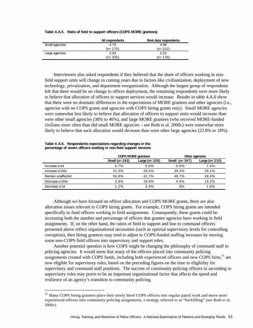
Hiring, Training, and Retention of Police Officers: A National Examination of Patterns and Emerging Trends 53
Table 4.A.5. Ratio of field to support officers (COPS MORE grantees)
All respondents Best data respondentsSmall agencies 4.76
(n=275)4.88
(n=102)Large agencies 3.93
(n=335)3.25
(n=139)
Interviewers also asked respondents if they believed that the share of officers working in non-field support units will change in coming years due to factors like civilianization, deployment of newtechnology, privatization, and department reorganization. Although the largest group of respondentsfelt that there would be no change in officer deployment, the remaining respondents were more likelyto believe that allocation of officers to support services would increase. Results in table 4.A.6 showthat there were no dramatic differences in the expectations of MORE grantees and other agencies (i.e.,agencies with no COPS grants and agencies with COPS hiring grants only). Small MORE agencieswere somewhat less likely to believe that allocation of officers to support units would increase thanwere other small agencies (38% to 46%), and large MORE grantees (who received MORE-fundedcivilians more often than did small MORE agencies – see Roth et al. 2000c) were somewhat morelikely to believe that such allocation would decrease than were other large agencies (22.8% to 18%).
Table 4.A.6. Respondents expectations regarding changes in thepercentage of sworn officers working in non-field support services
COPS MORE grantees Other agenciesSmall (n=243) Large (n=328) Small (n=367) Large (n=210)
Increase a lot 6.7% 5.0% 6.6% 7.4%Increase a little 31.3% 29.5% 39.4% 26.1%
Remain unaffected 56.8% 42.7% 48.7% 48.4%
Decrease a little 3.9% 18.9% 4.5% 16.2%Decrease a lot 1.2% 3.9% .8% 1.8%
Although we have focused on officer allocation and COPS MORE grants, there are alsoallocation issues relevant to COPS hiring grants. For example, COPS hiring grants are intendedspecifically to fund officers working in field assignments. Consequently, these grants could beincreasing both the number and percentage of officers that grantee agencies have working in fieldassignments. If, on the other hand, the ratios of field to support and line to command officerspresented above reflect organizational necessities (such as optimal supervisory levels for controllingcorruption), then hiring grantees may tend to adjust to COPS-funded staffing increases by movingsome non-COPS field officers into supervisory and support roles.
Another potential question is how COPS might be changing the philosophy of command staff inpolicing agencies. It would seem that many of the officers placed into community policingassignments created with COPS funds, including both experienced officers and new COPS hires,35 arenow eligible for supervisory roles, based on the preceding figures on the time to eligibility forsupervisory and command staff positions. The success of community policing officers in ascending tosupervisory roles may prove to be an important organizational factor that affects the speed andresilience of an agency’s transition to community policing.
35 Many COPS hiring grantees place their newly hired COPS officers into regular patrol work and move moreexperienced officers into community policing assignments, a strategy referred to as “backfilling” (see Roth et al.2000c).

54 Chapter 4
Retention of Staff Positions Funded Through the Federal COPS Program: 55Comparing Retention Rates Among COPS Agencies to Historical Patterns of Staff Retention in Police Agencies
CHAPTER 5.
Retention of Staff Positions FundedThrough the Federal COPS Program:Comparing Retention Rates AmongCOPS Agencies to Historical Patternsof Staff Retention in Police AgenciesChristopher S. Koper and Gretchen E. Moore, With David E. Huffer
One of the most ambitious crime policy initiatives of recent years has been the federalgovernment’s Community Oriented Policing Services (COPS) program. Passed as part of the ViolentCrime Control and Law Enforcement Act of 1994, a primary objective of the COPS program is to add100,000 additional police to the nation’s communities. One mechanism for achieving this is hiringgrants that generally fund up to 75% of the salary and fringe benefits of new officers for three years.When the federal government reached the milestone of funding 100,000 officers in May 1999(additional officers have been awarded since that time), approximately 61,000 of these officers hadbeen funded through hiring grants (the remainder had been funded through grants to improve officerproductivity by means of new technology and civilian positions).
The long-term impact of COPS on sworn force levels in the United States will be heavilyinfluenced by the extent to which grantees retain COPS-funded positions after the grants expire. Inother words, how much of the staffing increase funded by COPS will prove to be temporary and howmuch will last permanently, or at least indefinitely? The first part of this chapter assesses retention ofCOPS-funded positions using survey data gathered from a random sample of over 600 COPS granteeagencies (of all sizes and types) that were awarded COPS hiring grants in 1995 or earlier and that wereinterviewed by telephone for the Police Hiring and Retention (H&R) Survey in the summer of 2000(see the Methodological Appendix). The updated survey data permit an assessment of both actualretention patterns for positions funded by expired COPS grants and expected retention patterns forpositions that are still covered by COPS funding requirements.
As will be shown below, most COPS grantees have retained or expect to retain their COPS-funded positions, but a notable minority will not maintain their COPS-funded staffing increases. Thismay not prevent COPS from adding 100,000 more officers to the nation’s police forces on a temporaryor permanent basis, but it does imply that COPS will need to fund more than 100,000 officers toachieve a lasting increase of 100,000 officers. Should we view this as a failure of the COPS program?
Judging the success or failure of COPS in creating stable increases in police staffing can arguablybe facilitated by reference to historical patterns of staff retention following periods of police growth.If, for example, an agency increases its sworn force from 100 to 110 officers, how long should weexpect the agency to maintain a force of 110 or more officers based on historical norms? How longshould we expect the agency to maintain a force greater than its baseline level of 100 officers? Thesecond section of this chapter investigates these questions using national data on police employmentfrom 1975 through 1994, a period prior to the start of COPS. We then conclude by contrastingretention rates among COPS grantees to historical patterns of staff retention. Based on the limited

56 Chapter 5
data available at this time, it appears that, overall, observed and expected retention rates among COPSgrantees are consistent with what we would expect based on historical patterns.
5.1. RETENTION OF STAFFING INCREASES FUNDED BY COPS HIRING GRANTS
As noted above, COPS hiring grants are three-year awards. After a grant expires, COPS awardregulations stipulate that the grantee must keep the COPS-funded position(s) for one full budget cycle(generally, one year) following the budget cycle in which the grant expires. Using data gatheredduring the H&R survey, we examine both current retention of positions funded with expired COPSgrants and expected retention of positions still covered by either COPS funding or COPS retentionrequirements. H&R survey interviewers administered the COPS retention questions to 638 policeagencies that were sampled from among year 1995 COPS hiring grantees (see the MethodologicalAppendix).36 These agencies were chosen because they were among the earliest COPS grantees and,consequently, were more likely to have expired grants than were later cohorts of hiring grantees.
Note that in all analyses for this chapter, our focus is upon the retention of positions, irrespectiveof the particular officers filling those positions. For the COPS retention analyses, we countedpositions as retained (or likely to be retained) only if they had not been cut (or were not expected to becut) and had not been retained by cutting or using vacancies in non-COPS positions (or were notexpected to be retained through such means). By these criteria, an agency with five expired COPSpositions that reported keeping all five positions through cuts in other positions would not qualify as atrue retaining agency. Hence, our focus is on the full or partial retention of staffing increases that wereachieved with COPS funds. In other words, does it appear that an agency that had n officers andreceived a grant for k COPS officers will retain n+k officers or retain at least more than n officers afterthe expiration of its COPS grant?
5.1.1. Short-Term Retention of Positions Funded by Expired Grants
Among the 638 agencies that were questioned about COPS hiring grants during the H&R survey,374 (63% weighted) had one or more expired COPS grants. For 185 of these agencies, all COPSgrants were expired. As noted earlier, however, COPS grantees are required to keep positions for onefull budget cycle following the budget cycle in which the positions expire. Hereafter, we use the term“programmatically expired positions” to refer to expired COPS positions that have been expired forlonger than a full budget cycle and are thus eligible for cutting. Only 277 of the surveyed agencies(49% weighted) had programmatically expired COPS positions. Of this group, 213 agencies were nolonger required to keep any of their COPS-funded positions.
To determine whether the staffing increases produced by COPS grants had been maintained,interviewers inquired as to whether programmatically expired COPS positions had been cut. If thepositions had not been cut, interviewers asked whether the agency had kept any of the COPS positionsby cutting non-COPS positions or by using vacancies that opened up through the departure of officersin non-COPS positions.
As shown in table 5.1, about 12% of large agencies and 20% of small agencies withprogrammatically expired COPS positions had cut some or all of these positions (as in the otherchapters in this volume, we classify large agencies as those serving jurisdictions with 50,000 or morepersons and classify small agencies as those serving jurisdictions with fewer than 50,000 persons). Inaddition, nearly 13% of large agencies and nearly 9% of small agencies indicated keeping COPSpositions through cuts or attrition involving non-COPS positions.
36 These agencies were in the COPS FAST/AHEAD and COPS UHP strata of the H&R survey (see theMethodological Appendix).

Retention of Staff Positions Funded Through the Federal COPS Program: 57Comparing Retention Rates Among COPS Agencies to Historical Patterns of Staff Retention in Police Agencies
Agencies that had cut COPS positions were questioned about the reasons for these cuts. Overall,14% of the agencies with programmatically expired COPS positions had cut some or all of thosepositions. Interviewers questioned respondents for these agencies about possible reasons for the cuts.Echoing findings discussed elsewhere in this volume, nearly half of the agencies cutting positionscited economic/financial reasons for the cuts, but none of the agencies cited crime reduction as a factor(see table 5.2).37
The key numbers reflecting retention of COPS-funded staffing increases are shown in the fourthand fifth rows of table 5.1. Note that based on the timing of the H&R survey, we can expect that theprogrammatically expired positions had been so since only 1999 or early 2000 (in some cases, perhapsas early as 1998).38 Consequently, the retention figures represent short-term retention rates. Three-quarters of large agencies and just over 72% of small agencies with programmatically expired COPSpositions indicated that they had kept all of their COPS positions without making cuts or usingattrition of non-COPS positions. In other words, about three-quarters of large and small agencies hadfully retained the staffing increases funded by COPS. The figures change very little when consideringpartial retention of COPS-funded staffing increases; that is, virtually all COPS grantees retainingCOPS positions without cuts or attrition reported keeping all COPS positions.39
Table 5.1. COPS grantees' experiences with retention of programmatically expired cops positions*
Large agencies(n=116)
Small agencies(n=152)**
Cut some or all COPS positions 11.2% 20.2%
Keeping some or all COPS positions through cuts or attrition 12.6% 8.6%
Keeping some or all COPS positions using other grants*** 1.2% 0.2%
Keeping all COPS positions without cuts or attrition (full retention ofstaffing increases)
75.0% 72.2%
Keeping some or all COPS positions without cuts or attrition (full orpartial retention of staffing increases)
75.5% 73.4%
* Categories are not mutually exclusive. Retention status was unclear for 4% of large agencies and 6% of small agencies.
** Excludes nine agencies that had received supplemental COPS grants (under the Small Communities Grant Program) to assist small agencieswith retention.
*** Agencies with all programmatically expired positions on other grants were not counted as retaining agencies because the positions were notyet on the agencies' base budgets.
37 We did not run these analyses separately for large and small agencies due to the small sample size. Twenty-five of the thirty-three agencies were small agencies.38 A few thousand of the earliest COPS hiring grants were awarded in late 1993 and 1994 under the PoliceHiring Supplement (PHS) and COPS Phase I grant programs (Gaffigan et al. 2000). If the sampled agencies hadsuch grants, they may have expired programmatically prior to 1999.39 For these analyses, we treat all COPS awards granted to an agency as one staffing increase. Our data do notpermit the calculation of retention rates for each individual COPS grant awarded to an agency with multiplegrants. Likewise, these figures do not refer to the percentage of individual COPS positions that have beenretained. An assessment of the number of COPS positions that have been retained (and the number that arelikely to be retained in the future) will be presented as part of a separate, forthcoming report which will updateearlier estimates of the COPS program's impact on sworn force levels throughout the nation (Koper and Roth2000).

58 Chapter 5
Table 5.2. Reasons for discontinuing programmatically expired COPS-funded positions (n=33)
Reason % Saying reason was applicable
New political administration with new priorities came into office 10.5%
Jurisdiction experienced decrease in crime and needed fewer officers 0%
Fiscal constraints 48.6%
Other reasons 40.8%
5.1.2. Retention Projections for COPS Positions Not Programmatically Expired
When applicable, respondents were also questioned about whether they expected their agencies tokeep COPS positions that had not programmatically expired (i.e., positions that had not expiredfinancially and/or were still covered by the federal one budget cycle retention requirement). Overall,12% to 13% of COPS grantees expect to cut some or all of their COPS positions when the grantsexpire (table 5.3). About 21% of agencies expect to cut non-COPS positions or use attrition to retainsome or all of their COPS positions.
The key short-term retention figures are presented in the third and fourth rows of table 5.3. Justover two-thirds of both small and large COPS grantees expect to maintain COPS-funded staffingincreases in full without cutting other positions or using attrition. Seventy-four percent of small COPSagencies and eighty percent of large COPS agencies expect to retain at least some COPS positionswithout cuts or attrition.
Respondents were also questioned about the length of time that their agencies expect to keepthese positions (see bottom two rows of table 5.3). Virtually all of the large agencies expecting tomaintain COPS positions expect to maintain these positions for five or more years, regardless ofwhether they expect to retain all or just some of the positions. Small agencies expect some drop intheir long-term retention rates. For example, 73.9% of small agencies expect to keep at least some oftheir positions for the short-term, but a little less than 68% expect to keep at least some of theirpositions for as long as 5 years. Nonetheless, by either definition of retention (full or partial), over90% of small retaining agencies expect to retain their positions for the long term.40
The preceding analyses demonstrate that observed and expected retention rates among COPSgrantees are high but certainly not perfect. How might we judge these retention rates? Should weview them as evidence of success or failure? One way that we might begin to answer these questionsis to put COPS retention rates into an appropriate context. More specifically, we might ask whetherretention rates among COPS agencies are consistent with normal practice. Accordingly, the nextsection examines typical retention patterns in police agencies over the course of 20 years.
40 The observed and expected retention rates reported here are better than those reported in an earlier evaluationof the COPS program. Preliminary projections based on survey data gathered in the summer of 1998 suggestedthat more than half of grantees might fail to retain at least some of their COPS-funded staffing increases (Roth etal. 2000c, pp. 112-113). Methodological differences between this and the earlier study (e.g., differences in thegroups of agencies surveyed) and differences in the respondents’ levels of experience with expired or nearlyexpired COPS grants at the time of the two surveys probably account for some of the differing results. It alsoseems likely that grantees are currently more informed about COPS retention requirements. At the time of theearlier survey, the one budget cycle retention requirement had not been clearly established. Further, the federalCOPS Office (the agency that administers COPS grants) has recently undertaken efforts to improve grantees’understanding of programmatic retention requirements, including the stipulation that grantees should use COPSfunds to supplement, and not supplant, local funds (i.e., grantees should not retain COPS positions by cutting orfailing to fill other positions).

Retention of Staff Positions Funded Through the Federal COPS Program: 59Comparing Retention Rates Among COPS Agencies to Historical Patterns of Staff Retention in Police Agencies
Table 5.3. COPS grantees' expectations regarding future retentionof cops positions not yet programmatically expired
Large agencies(n=238)
Small agencies(n=286)
Cutting some or all COPS positions. 13.4% 12.2%
Keeping some or all COPS positions through cuts or attrition. 20.8% 21.4%
Keeping all COPS positions without cuts or attrition (full retention ofstaffing increases).
67.3% 68.0%
Keeping some or all COPS positions without cuts or attrition (full orpartial retention of staffing increases).
79.7% 73.9%
Keeping all COPS positions without cuts or attrition (full retention ofstaffing increases) for 5 or more years.
66.7% 62.6%
Keeping some or all COPS positions without cuts or attrition (full orpartial retention of staffing increases) for 5 or more years.
77.9% 67.5%
5.2. HISTORICAL PATTERNS OF STAFF RETENTIONFOLLOWING PERIODS OF AGENCY GROWTH
In this section, we investigate historical patterns of staff retention in police agencies using 20years of police employment data reported by state and local law enforcement agencies to the FederalBureau of Investigation's Uniform Crime Reports (UCR).41 Our objective is to determine how longagencies typically retain new positions following periods of growth. The analysis is based on 8,365agencies that reported employment data with sworn officer counts to the UCR for each year from 1975to 1994 and that experienced one or more moderate to large staffing increases from 1976 to 1993. Weidentified such staffing increases by examining the agencies' annual changes in sworn force. For eachoccasion when an agency experienced a substantial staffing increase, we tracked the agency'ssubsequent annual sworn force levels through 1994 to determine how long the agency maintainedsome or all of that staffing increase. We selected 1994 as the last tracking year because the COPSprogram began that year. We conducted survival analyses (Allison 1995) with these data to gaugetypical retention patterns.
As for most analyses presented in this report, we classified agencies as small or large based on thepopulation of each agency's jurisdiction. In order to focus on changes in agency size that seemed morelikely to represent meaningful, planned changes (rather than fluctuations due to annual turnover), weselected staffing increases of 20% or more for small agencies and 5% or more for large agencies.42
We also chose these levels because COPS hiring awards through year 2000 have averaged, in sum, 5%of the sworn force size of large grantees and 24% of the sworn force size of small grantees; 43 hence,the historical analysis is based on staffing increases approximately as large or larger than thosetypically funded by COPS.
41 We obtained the data from the UCR's annual Law Enforcement Officers Killed and Assaulted files, which arepublicly archived by the Inter Consortium for Political and Social Science Research. The analyses are based onactual sworn force levels as opposed to authorized or budgeted sworn force levels, which are not readilyavailable.42 We selected larger percentage increases for small agencies because percentage changes tend to be morevolatile in agencies with small numbers of officers.43 These figures are based on an analysis of grant records from the federal Office of Community OrientedPolicing Services (the agency which administers COPS grants).

60 Chapter 5
Using these criteria, we identified 19,364 staffing increases in small agencies and 4,565 staffingincreases in large agencies.44 The staffing increases averaged 54% for small agencies and 20% for largeagencies. The survival time for each staffing increase corresponds to the number of years that theagency maintained the new staffing level (or retained at least some portion of the staffing increase). Ifthe agency retained the new staffing level through 1994, then the case was censored at 1994. Forcensored cases, we know only that the higher staffing level was maintained through at least 1994.45
The first set of analyses examines full retention of staffing increases. If, for example, an agencywith n officers grows to n+k officers, how long does the agency maintain a force of at least n+kofficers? Table 5.4 presents the probabilities that staffing increases are maintained for selected lengthsof time based on the estimation of survival functions (see Allison 1995, pp. 9-60). To illustrate, thechance that a staffing increase is maintained in full for at least a year after its occurrence is 63% forsmall agencies and 66% for large agencies. By the fifth year following a staffing increase, thesefigures decline to 37% and 47% for small and large agencies, respectively. Therefore, less than half ofstaffing increases in police agencies are maintained fully for at least five years, based on the staffingincrease criteria used in these analyses. The full survivor functions for small and large agencies areillustrated graphically in figures 5.1 and 5.2.
Agencies are most likely to fail at maintaining full staffing increases during the first few yearsafter the staffing increase occurs. The longer the agency maintains the higher staffing level, the morelikely it is that the new staffing level will be maintained indefinitely (hence, the survival curves infigures 5.1 and 5.2 become flatter over time). This might suggest that agencies tend to raise staffinglevels in advance of expected attrition so that the target staffing level is equal to the increase of kofficers minus some number of officers that are expected to depart.
The data provide some indications that large agencies are more likely to fully maintain staffingincreases than are small agencies, but such inferences may be contingent on the magnitudes of thestaffing increases chosen for analysis. A 5% staffing increase in a large agency may not affect theagency in the same way that a 20% staffing increase affects a small agency. Moreover, large andsmall agency comparisons are not central to the research question under study.
Table 5.4. Probabilities that staffing increases will be retainedin full for selected lengths of time by agency size
Timein years
Small agencies(n=19,364 staffing increases)
Large agencies(n=4,565 staffing increases)
1 year .63 .66
2 years .50 .563 years .44 .52
4 years .40 .49
5 years .37 .47
10 years .30 .4415 years .28 .42
44 Note that any given agency may have had multiple staffing increases incorporated into the analysis.45 Of course, the potential follow-up time varied according to when the staffing increase occurred. A staffingincrease occurring from 1975 to 1976 had 18 years of potential follow-up before censoring. In contrast, astaffing change occurring from 1992 to 1993 had one potential year of follow-up.

Retention of Staff Positions Funded Through the Federal COPS Program: 61Comparing Retention Rates Among COPS Agencies to Historical Patterns of Staff Retention in Police Agencies
Figure 5.1. Probability that small agencies retain staffing increasesin full, by years of follow-up
0
0.2
0.4
0.6
0.8
1
1.2
0 1 2 3 4 5 6 7 8 9 10 11 12 13 14 15 16 17 18
Duration
Su
rviv
al D
istr
ibu
tio
n F
un
ctio
n
Figure 5.2. Probability that large agencies retain staffing increasesin full, by years of follow-up
0
0.2
0.4
0.6
0.8
1
1.2
0 1 2 3 4 5 6 7 8 9 10 11 12 13 14 15 16 17 18
Years
Su
rviv
al D
istr
ibu
tio
n F
un
ctio
n
Further analyses revealed that full retention varies by the size of the staffing increase. As shownin tables 5.5 and 5.6, staffing increases are more likely to be maintained in full in both small and largeagencies when they are more modest in size.

62 Chapter 5
Table 5.5. Probabilities that staffing increases will be retainedin full for selected lengths of time by size of staffing increase (small agencies)
Time in Years Increases Below Median:20% to 33%
(n=8,263 staffing increases)
Increases Above Median: >33%(n=11,101 staffing increases)
1 year .66 .612 years .54 .483 years .48 .414 years .44 .365 years .41 .3410 years .35 .2715 years .33 .25
Table 5.6. Probabilities that staffing increases will be retainedin full for selected lengths of time by size of staffing increase (large agencies)
Timein years
Increases below median:5% to 9.8%
(n=2,290 staffing increases)
Increases above median:>9.8%
(n=2,275 staffing increases)1 year .68 .632 years .59 .543 years .55 .494 years .52 .465 years .50 .4410 years .47 .4115 years .45 .40
In a second set of analyses, we estimated the probability that an agency maintains at least some ofa staffing increase for selected periods of time. If, in other words, an agency increases its force from nofficers to n+k officers, how long does the agency maintain any staffing level higher than its baselinelevel of n? Using this criterion, agencies are much more successful at retaining staffing growth (seetable 5.7). The chance that an agency will retain some of its growth for at least a year is 92% for largeagencies and 81% for small agencies. The five-year maintenance rate is 79% for large agencies and59% for small agencies. As in the previous analyses, the likelihood that an agency fails to maintain astaffing increase is greatest during the period immediately following the increase. Also, there areagain tentative indications that large agencies are more successful at retaining new positions, subject tothe caveats noted above. Indeed, 72% of staffing increases in large agencies last in at least someresidual form for 15 years. Figures 5.3 and 5.4 illustrate the survivor functions.
Table 5.7. Probabilities that staffing increases will be retainedpartially for selected lengths of time by agency size
Timein years
Small agencies(n=19,364 staffing increases)
Large agencies(n=4,565 staffing increases)
1 year .81 .922 years .72 .873 years .66 .834 years .62 .805 years .59 .7910 years .51 .7415 years .48 .72

Retention of Staff Positions Funded Through the Federal COPS Program: 63Comparing Retention Rates Among COPS Agencies to Historical Patterns of Staff Retention in Police Agencies
Figure 5.3. Probability that small agencies retain staffing increasespartially or fully, by years of follow-up
0
0.2
0.4
0.6
0.8
1
1.2
0 1 2 3 4 5 6 7 8 9 10 11 12 13 14 15 16 17 18
Years
Su
rviv
al D
istr
ibu
tio
n F
un
ctio
n
Figure 5.4. Probability that large agencies retain staffing increasespartially or fully, by years of follow-up
0
0.2
0.4
0.6
0.8
1
1.2
0 1 2 3 4 5 6 7 8 9 10 11 12 13 14 15 16 17 18
Years
Su
rviv
al D
istr
ibu
tio
n F
un
ctio
n
The size of the staffing increase is not strongly related to this weaker form of retention. Amongsmall agencies, the survivor functions for staffing increases above and below the median do not differsignificantly. For large agencies, the differences are statistically significant but modest. Thedifferences are most notable at longer follow-up times. For example, staffing increases above themedian have a .81 probability of retention to 5 years, while those below the median have a probability

64 Chapter 5
of .76. (This may suggest that larger staffing increases are more indicative of meaningful, plannedstaffing changes in large agencies.)
To conclude, this investigation has revealed some basic patterns of staff retention in policeagencies following periods of agency growth. One conclusion is that it is not uncommon for agenciesto fail to retain staffing increases for more than a few years. This is particularly true for full retentionof staffing increases. In general, agencies are less likely than not to retain full staffing increases formore than just a few years following implementation. In most instances, however, they retain someresidual of those increases for five or more years. A second general point is that agencies are atgreatest risk of retention failure in the first few years after a staffing increase. If an agency manages toretain new positions for at least a few years following the staffing increase, it becomes much morelikely that the agency will retain the new positions for the long term.
A number of caveats should be noted. As discussed above, this inquiry is based on a group ofbetween 8,000 and 9,000 agencies that experienced staffing increases and reported employment dataannually to the UCR from the mid-1970s to the mid-1990s. We cannot say if or how retentionpatterns differ for this subset of agencies and the full universe of police agencies.46
In addition, it is likely that various agency characteristics and external social factors, such aseconomic conditions, crime trends, and the availability of grant money, affect retention patterns.Testing such hypotheses is beyond the scope of this exploratory investigation. 47 Nonetheless, theseanalyses reveal typical retention patterns net of various influences over parts or all of three differentdecades, and they provide a basis for initial comparisons to the COPS retention rates described earlier,which were also presented net of other social influences.
46 For some agencies and years, staffing levels listed in the UCR are those reported by agencies in the prior year.If such records do not reflect staffing levels accurately, they could potentially bias the types of analysespresented here by introducing error into both the identification of staffing increases (in terms of timing andmagnitude) and the measurement of survival periods. The analyses presented in the text are based on whateverstaffing levels were reported in the UCR and assume that those levels are accurate (i.e., if the data for agency x,year t indicated that agency x's sworn force count was from the prior year, we assumed that agency x did notchange in size from year t-1 to year t).
To test the sensitivity of the analyses to this assumption, we identified staffing increases and follow-upperiods that were potentially contaminated by this possible source of measurement error. (For each agency, weidentified the last year up through 1994 in which the UCR listed data from a prior year. For an agency whosemost recent questionable data year was year t, we flagged all staffing increases and follow-up periods occurringup through year t+1 as potentially contaminated observations.) This resulted in the loss of 24% of theobservations used in the main analyses. We re-estimated the basic survival functions presented in figures 5.1through 5.4 without these potentially contaminated cases. The alternative estimates differed little from thosepresented in the text. To illustrate, the survival probabilities for partial maintenance of staffing increases in largeagencies were .93 at year 1, .80 at year 5, and .76 at year 10. For small agencies, the comparable values were.81, .60, and .52. All of these values are nearly identical to those presented in table 5.7.47 However, we conducted tentative analyses on two additional factors: agency type and decade when thestaffing increase occurred. A number of basic univariate tests indicated that staffing increases are more likely tobe maintained in county and municipal agencies and less likely to be maintained in sheriffs’ agencies. We alsofound some indications that staffing retention has improved over time. In general, retention was somewhathigher in the 1980s and early 1990s than in the 1970s.
For the latter analyses, we compared survival functions for staffing increases occurring during the1970s and 1980s (we excluded the 1990s due to the short follow-up periods available for observations from thatdecade). In addition, we contrasted 2-year survival rates for staffing increases occurring during 1970s, 1980s,and early 1990s (1990-1992). For example, the probabilities that staffing increases would be maintained in partfor two years in small agencies were 69%, 72%, and 75% for, respectively, those occurring during the 1970s,1980s, and early 1990s. The comparable figures for large agencies were 82%, 88%, and 89%.

Retention of Staff Positions Funded Through the Federal COPS Program: 65Comparing Retention Rates Among COPS Agencies to Historical Patterns of Staff Retention in Police Agencies
5.3. COMPARING RETENTION RATES AMONG COPS GRANTEES TO HISTORICALRETENTION PATTERNS
For comparative purposes, the observed retention rates for COPS agencies with programmaticallyexpired COPS positions and the initial, post-expiration (i.e., short-term) retention rates expected foragencies with non-expired COPS positions should be most comparable to the 1-2 year retention ratesin the historical analysis. For long-term assessments, we can compare the expected 5-year retentionrates for COPS agencies to the historical 5-year patterns.
Relative to historical patterns, full retention of staffing increases appears to be greater amongCOPS grantees. For example, 72% of small agencies with programmatically expired COPS positionsand 75% of corresponding large agencies have retained all of their expired COPS positions. Based onhistorical patterns, in contrast, we would expect only 50% to 63% of small agencies and 56% to 66%of large agencies to retain all new positions.
However, these comparisons are likely to be misleading. As shown in the historical analysis, fullretention of a staffing increase is sensitive to the size of the staffing increase – the larger the increase,the less likely it is that the agency will maintain the new staffing level in full for any given length oftime. Because the staffing changes analyzed in the historical study tended to be substantially largerthan COPS-funded staffing increases, the preceding comparisons have a bias in favor of COPS.
Partial retention of staffing increases, on the other hand, tends to be less sensitive to the magnitudeof the staffing change (see previous section) and may therefore provide a more reliable means ofcomparing COPS and historical retention patterns. Table 5.8 presents a series of comparisons using thisless restrictive retention criterion. The range of short-term (i.e., 1-2 year) estimates for COPS grantees intable 5.8 is based on both observed retention rates for expired COPS positions and expected short-termretention rates for non-expired COPS positions. The long-term (i.e., five-year) projections for COPSgrantees are based on expectations about the retention of non-expired positions.
Table 5.8. Retention of cops-funded positions (actual and expected) compared to historical norms: Probabilitiesthat at least some new positions are retained for selected follow-up periods
Small agencies Large agencies
COPS Historical COPS Historical
1-2 years 73%-74%* 72%-81% 75%-80%* 87%-92%
5 years 68%** 59% 78%** 79%
* Ranges based on short-term retention experience with expired grants and short-term retention projections for non-expired grants(see tables 5.1 and 5.3).
** Based on long-term retention projections for non-expired grants (see table 5.3).
Overall, the estimates in table 5.8 suggest that retention rates among COPS grantees will becomparable to historical patterns. Retention rates among small COPS agencies will be consistent withhistorical patterns in the short-term and better than historical patterns in the long-term. Retention ratesfor large COPS agencies will be somewhat lower than historical projections in the short-term but areexpected to be virtually identical to historical patterns in the long-term.
These comparisons should be treated cautiously because they are based largely on the futureexpectations of COPS grantees; only a relatively small fraction of COPS agencies had actualexperience with retention of programmatically expired COPS grants by the time of the H&R survey.Further, the historical investigation was of necessity a somewhat crude method of identifying andanalyzing staffing changes in police agencies. But based on the limited data available at this time, wecan say cautiously that retention rates among COPS grantees, while not perfect, will be comparable tohistorical norms of staff retention in police agencies. If COPS grantees’ projections prove accurate,then it seems that money invested in raising police staffing levels through COPS grants will produce areturn on investment comparable to the usual return on investments to raise police staffing levels.

66 References
References
Allison, Paul. 1995. Survival Analysis Using theSAS System: A Practical Guide. Cary, NC:SAS Institute.
Bahl, Roy W., Richard D. Gustely, and Michael J.Wasylenko. 1978. “The Determinants of LocalGovernment Police Expenditures: A PublicEmployment Approach.” National Tax Journal31:67-79.
Bayley, David H. 1985. Patterns of Policing: AComparative International Analysis. NewBrunswick, NJ: Rutgers University Press.
Bayley, David H. 1994. Police for the Future. NewYork: Oxford University Press.
Bordua, David J. and Edward W. Haurek. 1970.“The Police Budget’s Lot: Components of theIncrease in Local Police Expenditures, 1902-1960.” American Behavioral Scientist 13:667-680.
Brandl, Steven G., Mitchell B. Chamlin, and JamesFrank. 1995. “Aggregation Bias and theCapacity for Formal Crime Control: TheDeterminants of Total and DisaggregatedPolice Force Size in Milwaukee, 1934-1987.”Justice Quarterly 12:543-562.
Butterfield, Fox. 2001. “Urban Police Jobs AreLosing Their Appeal.” The New York TimesJuly 30 (accessed at www.nytimes.com).
Carr-Hill, R.A. and N.H. Stern. 1973. “AnEconometric Model of the Supply and Controlof Recorded Offenses in England and Wales.”Journal of Public Economics 2:289-318.
Carr-Hill, R.A. and N.H. Stern. 1977. “Theory andEstimation in Models of Crime and its SocialControl and their Relations to Concepts ofSocial Output” In The Economics of PublicServices, edited by Martin S. Feldstein andRobert P. Inman. New York: Halsted Press.
Chaiken, Jan M. 1975. Patrol AllocationMethodology for Police Departments.California: Rand Corporation.
Chamlin, Mitchell B. 1990. “Determinants ofPolice Expenditures in Chicago, 1904-1958.”The Sociological Quarterly 31:485-494.
Chamlin, Mitchell B. and Robert H. Langworthy.1996. “The Police, Crime, and EconomicTheory: A Replication and Extension.”American Journal of Criminal Justice 20:165-182.
Chapman, Jeffrey I. 1976. “An Economic Model ofCrime and Police: Some Empirical Results.”Journal of Research in Crime and Delinquency13:48-63.
Cloninger, Dale O. and Lester C. Sartorius. 1979.“Crime Rates, Clearance Rates andEnforcement Effort: The Case of Houston,Texas.” American Journal of Economics andSociology 38(4): 389-402.
Corman, Hope, Theodore Joyce, and NormanLovitch. 1987. “Crime, Deterrence and theBusiness Cycle in New York: A VARApproach.” The Review of Economics andStatistics 69:695-700.
Corman, Hope and Theodore Joyce. 1990. “UrbanCrime Control: Violent Crimes in New YorkCity. Social Science Quarterly, 71:567-584.
Craig, Steven G. 1987. “The Deterrent Impact ofPolice: An Examination of a Locally ProvidedPublic Service.” Journal of Urban Economics21:298-311.
Dye, Thomas R. 1976. Policy Analysis: WhatGovernments Do, Why They Do It, and WhatDifference in Makes. Alabama: University ofAlabama Press.
Eck, John and Edward R. Maguire. 2000. “HaveChanges in Policing Reduced Violent Crime?An Assessment of the Evidence.” In The CrimeDrop in America, edited by Alfred Blumsteinand Joel Wallman (207-265). New York:Cambridge University Press.
Fisher, Franklin M. and Daniel Nagin. 1978. “Onthe Feasibility of Identifying the CrimeFunction in a Simultaneous Model of CrimeRates and Sanction Levels.” In Deterrence andIncapacitation: Estimating the Effects ofCriminal Sanctions on Crime Rates, edited byAlfred Blumstein, Jacqueline Cohen, andDaniel Nagin (361-399). Washington, DC:National Academy of Sciences.

References 67
Fox, James Alan. 1978. Forecasting Crime Data:An Econometric Analysis. Massachusetts:Lexington Books.
Fujii, Edwin, and James Mak. 1980. “Tourism andCrime: Implications for Regional DevelopmentPolicy.” Regional Studies 14: 27-36.
Furlong, William J. and Stephen L. Mehay. 1981.“Urban Law Enforcement in Canada: AnEmpirical Analysis.” The Canadian Journal ofEconomics XIV(1):44-57.
Gaffigan, Stephen J., Jeffrey A. Roth, and MichaelE. Buerger. 2000. “Origins and Objectives ofthe COPS Program.” In National Evaluation ofthe COPS Program - Title I of the 1994 CrimeAct (25-61). Washington, DC: NationalInstitute of Justice, U.S. Department of Justice.
Goldberg, Andrew L. and Brian A. Reaves. 2000.Sheriffs’ Departments 1997. Washington, DC:Bureau of Justice Statistics, U.S. Departmentof Justice. NCJ 173428.
Greenberg, David F. and Ronald C. Kessler. 1982.“Model Specification in Dynamic Analysis ofCrime Deterrence.” In DeterrenceReconsidered: Methodological Innovations.Beverly Hills, CA: Sage Publications.
Greenberg, David F., Ronald C. Kessler, and ColinLoftin. 1983. “The Effect of PoliceEmployment on Crime.” Criminology21(3):375-394.
Greenberg, David F., Ronald C. Kessler, and ColinLoftin. 1985. “Social Inequality and CrimeControl.” Journal of Criminal Law andCriminology 76:684-704.
Greenwood, Michael J. and Walter J. Wadycki.1973. “Crime Rates and Public Expendituresfor Police Protection: Their Interaction.”Review of Social Economy 31:138-152.
Hakim, Simon. 1980. “The Attraction of PropertyCrimes to Suburban Localities: A RevisedEconomic Model.” Urban Studies 17:265-276.
Hakim, Simon, Arie Ovadia, Eli Sagi, and J.Weinblatt. 1979. “Interjurisdictional Spilloverof Crime and Police Expenditure.” LandEconomics 55(2):200-212.
Hakim, Simon, Uriel Spiegal, and J. Weinblatt.1984. “Substitution, Size Effects, and theComposition of Property Crime.” SocialScience Quarterly 65:719-734.
Hickman, Matthew J. and Brian A. Reaves. 2001.Local Police Departments 1999. Washington,
DC: Bureau of Justice Statistics, U.S.Department of Justice. NCJ 186478.
Hirsch, Werner Z. 1959. “Expenditure Implicationsof Metropolitan Growth and Consolidation.”The Review of Economics and StatisticsXLI(3):232-241.
Huff, C. Ronald and John M. Stahura. 1980.“Police Employment and Suburban Crime.”Criminology 17:461-470.
Jackson, Pamela. 1992. “The Police and SocialThreat: Urban Transition, Youth Gangs, andSocial Control.” Policing and Society 2:193-204.
Jackson, Pamela and Leo Carroll. 1981. “Race andthe War on Crime: The SocipoliticalDeterminants of Municipal PoliceExpenditures in 90 Non-Southern U.S. Cities.”American Sociological Review 46:290-305.
Jacobs, David. 1979. “Inequality and PoliceStrength: Conflict Theory and CoerciveControl in Metropolitan Areas.” AmericanSociological Review 44(December):913-925.
Jacobs, David and Ronald E. Helms. 1997. “TestingCoercive Explanations for Order: TheDeterminants of Law Enforcement StrengthOver Time.” Social Forces 75(4):1361-1392.
Jones, E. Terrence. 1974. “The Impact of CrimeRate Changes on Police ProtectionExpenditures in American Cities.” Criminology11(4):516-524.
Koper, Christopher S. and Jeffrey A. Roth. 2000.“Putting 100,000 Officers on the Street:Progress as of 1998 and PreliminaryProjections Through 2003.” In NationalEvaluation of the COPS Program - Title I ofthe 1994 Crime Act (149-178). Washington,DC: National Institute of Justice, U.S.Department of Justice.
Land, Kenneth C. and Marcus Felson. 1976. “AGeneral Framework for Building DynamicMacro Social Indicator Models: Including anAnalysis of Changes in Crime Rates and PoliceExpenditures.” American Journal of Sociology82:565-604.
Langworthy, Robert, Thomas Hughes, and BethSanders. 1995. Law Enforcement Recruitment,Selection, and Training: A Survey of MajorPolice Departments in the U.S. HighlandHeights, KY: Police Section, Academy ofCriminal Justice Sciences.

68 References
Larson, Richard C. 1978. Police Deployment: NewTools for Planners. New York, NY: LexingtonBooks.
Law Enforcement News. 2000a. “Coast to Coast,Good Police Recruits Just Keep Getting Harderto Find.” May 15:1,15.
Law Enforcement News. 2000b. “NYPD Facing aFlood of 20-and-Out Retirees.” Feb. 14:5.
Levitt, Steven D. 1997. “Using Electoral Cycles inPolice Hiring to Estimate the Effect of Policeon Crime.” American Economic Review 87(3):270-91.
Liska, Allen E. and Mitchell B. Chamlin. 1984.“Social Structure and Crime Control amongMacrosocial Units.” American Journal ofSociology 90:383-397.
Liska, Allen E., Joseph J. Lawrence, and MichaelBenson. 1981. “Perspectives on the LegalOrder: The Capacity for Social Control.”American Journal of Sociology 87:413-426.
Lizotte, Alan J., James Mercy, and EricMonkkonen. 1982. “Crime and Police Strengthin an Urban Setting: Chicago, 1947-1970.” InQuantitative Criminology: Innovations andApplications, edited by John Hagan (129-148).Beverly Hills, CA: Sage Publications.
Loftin, Colin and David McDowall. 1982. “ThePolice, Crime, and Economic Theory: AnAssessment.” American Sociological Review47:393-401.
Lundman, Richard J. 1997. “Police Levels andCrime: Additional Evidence.” UnpublishedManuscript. Department of Sociology, OhioState University.
McDowall, David and Colin Loftin. 1986. “FiscalPolitics and the Police: Detroit, 1928-76.”Social Forces 65:162-176.
McPheters, Lee R. and William B. Stronge. 1974.“Law Enforcement Expenditures and UrbanCrime.” National Tax Journal 27:633-644.
Marvell, Thomas B. and Carlisle E. Moody. 1996.“Specification Problems, Police Levels, andCrime Rates.” Criminology 34:609-646.
Mathieson, Donald and Peter Passell. 1976.“Homicide and Robbery in New York City: AnEconomic Model.” Legal Studies 5(1):83-98.
Mehay, Stephen L. 1979. “IntergovernmentalContracting for Municipal Police Services: AnEmpirical Analysis.” Land Economics55(1):59-72.
Morris, Douglas and Luther Tweeten. 1971. “TheCost of Controlling Crime: A Study inEconomics of City Life.” The Annals ofRegional Science 5(1):33-49.
Nagin, Daniel S. 1978. “General Deterrence: AReview of the Empirical Evidence.” InDeterrence and Incapacitation , edited byAlfred Blumstein, Jacqueline Cohen, andDaniel Nagin (95-139). Washington, DC:National Academy of Sciences.
Nagin, Daniel S. 1998.“Criminal DeterrenceResearch at the Outset of the Twenty FirstCentury.” In Crime and Justice: A Review ofResearch, edited by Michael Tonry (vol. 23, 1-42). Chicago: University of Chicago Press.
Nalla, Mahesh K. 1992. “Perspectives on theGrowth of Police Bureaucracies, 1948-1984:An Examination of Three Explanations.”Policing and Society 3:51-61.
Nalla, Mahesh K., Michael J. Lynch, and MichaelJ. Leiber. 1997. “Determinants of PoliceGrowth in Phoenix, 1950-1988.” JusticeQuarterly 14(1):115-143.
Niskanen, William A. 1994. “Crime, Police, andRoot Causes.” Policy Analysis Number 218(November 14). Cato Institute.
O’Boyle, E.H. 1990. “Manpower: Meeting theDemands of a Growing Department.” TheExtra Mile 1(1): 1-7.
Phillips, Llad and Harold L.Votey, Jr. 1975. “CrimeControl in California.” The Journal of LegalStudies, IV(2):327-349.
Raub, R.A. 1984. Model to Allocate State PoliceManpower to Districts - Revised Version.Illinois Department of Law Enforcement.
Reaves, Brian A. 1996. Local Police Departments1993. Washington, DC: Bureau of JusticeStatistics, U.S. Department of Justice. NCJ148822.
Reaves, Brian A. and Andrew L. Goldberg. 1998.Census of State and Local Law EnforcementAgencies, 1996 . Washington, DC: Bureau ofJustice Statistics, U.S. Department of Justice.NCJ 164618.
Reaves, Brian A. and Andrew L. Goldberg. 1999.Law Enforcement Management andAdministrative Statistics, 1997: Data forIndividual State and Local Agencies with 100or More Officers . Washington, DC: Bureau ofJustice Statistics, U.S. Department of Justice.NCJ 171681.

References 69
Reaves, Brian A. and Andrew L. Goldberg. 2000.Local Police Departments 1997. Washington,DC: Bureau of Justice Statistics, U.S.Department of Justice. NCJ 173429.
Reaves, Brian A. and Matthew J. Hickman. 2001.Sheriffs’ Offices 1999. Washington, DC:Bureau of Justice Statistics, U.S. Departmentof Justice. NCJ 186479.
Reaves, Brian A. and Pheny Z. Smith. 1996.Sheriffs’ Departments 1993. Washington, DC:Bureau of Justice Statistics, U.S. Departmentof Justice. NCJ 148823.
Roehl, Janice A., Calvin C. Johnson, Michael E.Buerger, Stephen J. Gaffigan, Elizabeth A.Langston, and Jeffrey A. Roth. 2000. “COPSand the Nature of Policing.” In NationalEvaluation of the COPS Program - Title I ofthe 1994 Crime Act (179-245). Washington,DC: National Institute of Justice, U.S.Department of Justice.
Roth, Jeffrey A., Joseph F. Ryan, Stephen J.Gaffigan, Christopher S. Koper, Mark H.Moore, Janice A. Roehl, Calvin C. Johnson,Gretchen E. Moore, Ruth M. White, MichaelE. Buerger, Elizabeth A. Langston, and DavidThacher. 2000a. National Evaluation of theCOPS Program - Title I of the 1994 Crime Act.Washington, DC: National Institute of Justice,U.S. Department of Justice.
Roth, Jeffrey A., Calvin C. Johnson, GretchenMaenner, and Daryl E. Herrschaft. 2000b.“The Flow of COPS Funds.” In NationalEvaluation of the COPS Program - Title I ofthe 1994 Crime Act (63-100). Washington, DC:National Institute of Justice, U.S. Departmentof Justice.
Roth, Jeffrey A., Christopher S. Koper, Ruth White,and Elizabeth A. Langston. 2000c. “UsingCOPS Resources.” In National Evaluation ofthe COPS Program - Title I of the 1994 CrimeAct (101-148). Washington, DC: NationalInstitute of Justice, U.S. Department of Justice.
Slovak, Jeffrey S. 1986. Styles of Urban Policing:Organization, Environment, and Police Stylesin Selected American Cities. New York: NewYork University Press.
Snipes, Jeffrey B. 1993. “Issues and Refinements inModeling Macro-level Threat Theory.”Unpublished Manuscript. Department ofCriminal Justice, SUNY-Albany.
Sollars, David L., Bruce L. Benson, and David W.Rasmussen. 1994. “Drug Enforcement and theDeterrence of Property Crime among Local
Jurisdictions.” Public Finance Quarterly22(1):22-45.
Stenzel, W. 1993. Police Personnel AllocationManual User’s Guide: Determination of theNumber and Allocation of Personnel for Patroland Traffic Services for Municipal LawEnforcement Agencies. Chicago, IL:Northwestern University Traffic Institute.
Surette, Raymond. 1984. “A Note on the HistoricalRelationship Between the Economy and PoliceOrganizational Activities.” Criminal JusticeReview 9:47-52.
Swimmer, Gene. 1974a. “Measurement of theEffectiveness of Urban Law Enforcement: ASimultaneous Approach” Southern EconomicJournal 40:618-630.
Swimmer, Gene. 1974b. “The Relationship ofPolice and Crime: Some Methodological andEmpirical Results.” Criminology 12:293-314.
Victor, Michael L. 1977. “Relations BetweenKnown Crime and Police Spending in LargeUnited States Cities.” Sociological Focus10(2):199-207.
Walzer, Norman. 1972. “Economies of Scale andMunicipal Police Services: The IllinoisExperience.” Review of Economics andStatistics 431-438.
Weicher, John C. 1971. “The Allocation of PoliceProtection by Income Class.” Urban Studies207-220.
Wilson, James Q. and Barbara Boland. 1978. “TheEffect of Police on Crime.” Law and SocietyReview 12:367-390.
Wolpin, Kenneth I. 1978. “An Economic Analysisof Crime and Punishment in England andWales, 1894-1967.” Journal of PoliticalEconomy 86:815-840.

70 Methodological Appendix
METHODOLOGICAL APPENDIX.
The Police Hiring and Retention (H&R)Survey
A.1. OVERVIEW OF THE COPS-POLICE HIRING AND RETENTION SURVEY SAMPLE
From June through August of 2000, interviewers from the National Opinion Research Center(NORC) conducted telephone interviews with a nationally representative sample of 1,270 policeagencies. Each interview was conducted with the chief of police or a representative designated by thechief of police. Project staff selected and interviewed these agencies initially in 1996 as part of theUrban Institute's (UI) national evaluation of the COPS program (Roth et al. 2000a). Project staff re-interviewed these agencies during the summer of 2000 for an updated study of the COPS program.The follow-up interviews also included a series of questions pertaining to general hiring and retentionpractices (referred to throughout this volume as the H&R survey).
Key characteristics of the sample are presented in tables A.1 through A.3. The sample isstratified by jurisdiction size and COPS funding status and program type as of 1996 (the developmentof the survey design is discussed below). Large agencies are categorized as those serving jurisdictionsof 50,000 or more persons (see table A.1). The remaining agencies constitute the small agency group.COPS grantees and large agencies were sampled disproportionately due to, respectively, the survey'srole in the ongoing UI evaluation of the COPS program and the disproportionate concentration of thenation's police officers in large jurisdictions. The data were weighted to provide national estimates.The breakdown of COPS grantee status shown in table A.2 represents the agencies' grant status as ofyear 2000. By that time, 86% of the agencies were COPS grantees; 59% of the agencies had beenfunded with COPS hiring grants.48
As shown in table A.3, the majority of the agencies are municipal or county police agencies.Sheriffs’ agencies are the next most common agency type. State police and other miscellaneousagencies account for less than 10 percent of the sample.
Table A.1. Jurisdiction size of sample agencies (n=1,270)
SizeAverage
number of officers% of
sample% of
weighted sample
Large: population of 50,000 or more 361.4 43.5 5.0
Small: population less than 50,000 23.6 56.5 95.0
48 Some agencies changed COPS funding status from 1996 through 2000. In 1996, 293 of the agencies in thesample (23%) were not funded through the COPS program. By 2000, 175 of these agencies (14% of the sample)still did not have COPS funding. Only 2.8% of the agencies changed from being grantees in 1996 to non-grantees by 2000.

The Police Hiring and Retention (H&R) Survey 71
Table A.2. COPS grantee status of sample agencies (n=1,270)
% of sample % of weighted sample
COPS Grantee 86.2 62.5
Hiring Grantee 59.2 54.0
No COPS Grants 13.8 37.5
Table A.3. Agency types of sample agencies (n=1,270)*
% of sample % of weighted sample
Municipal / County 80.1 78.3
Sheriff 13.1 13.1
University or School Police 2.8 4.6
State Police 1.4 1.0
Other** 2.5 2.7
* Percentages may not add to 100 due to rounding.
** “Other” agencies include transit police, public housing police, park police, tribal police, and other miscellaneousagency types.
A.2. DEVELOPMENT OF THE SAMPLE DESIGN
The sample design is based on that developed in 1996 for the UI evaluation of the federal COPSprogram (Roth et al. 2000a). To create the 1996 sample, UI staff utilized records from the federalOffice of Community Oriented Policing Services (the COPS Office), the Uniform Crime Reports, andthe National Crime Information Center to develop a national list of nearly 21,000 law enforcementagencies eligible for COPS funding. These agencies were stratified according to COPS grant statusand jurisdiction size as follows (see table A.4).
Table A.4. Sampling frame by funding/program status and population category for 1996 cops survey*
Populationgroup
Agencies not fundedthrough COPS
COPS FAST-AHEADgrantees
COPS UHPgrantees
COPS MOREgrantees Total
Less than 50,000 8,373 5,845 1,186 1,136 16,54050,000 or more 267 546 159 349 1,321Missing 4,208 79 4,287Total 12,848 6,391 1,345 1,564 22,148
* Some agencies are counted more than once due to participation in multiple COPS grant programs.
The FAST/AHEAD and Universal Hiring Program (UHP) strata refer to different COPS hiringgrant programs. The MORE stratum corresponds to agencies which were funded to acquiretechnology or civilians and/or to pay overtime for additional patrol. 49
49 The size stratification point of 50,000 residents was based in part on administrative distinctions established forearly COPS grants. In late 1994, the COPS Office established the Funding Accelerated for Small Towns (FAST)program for agencies serving populations of 50,000 or less. The program had simplified application proceduresto speed processing. At the same time, the COPS Office established the Accelerated Hiring, Education, and

72 Methodological Appendix
UI staff sampled over 2,000 of these agencies for a first-wave interview in the fall of 1996. Thedesigned sampling fractions are shown below (table A.5). Based on substantive and statisticalconsiderations, project staff sampled disproportionately from among COPS grantees and largeagencies. Nonetheless, the sample is a nationally representative sample weighted to produce nationalestimates.
Table A.5. Designed sampling fraction by funding-program status andpopulation category for 1996 COPS Survey
Populationgroup
Agencies not fundedthrough COPS
COPS FAST-AHEADgrantees
COPS UHPgrantees
COPS MOREgrantees Total
Less than 50,000 0.013 0.048 0.236 0.248 0.05750,000 or more 1.0 0.498 1.0 0.777 0.734Missing 0.044 0.044Total 0.044 0.086 0.326 0.354 0.095
Table A.6 presents the response rates for the 1996 COPS survey.
Table A.6. Survey response rates by funding-program status andpopulation category (in percentages) for 1996 cops survey
Populationgroup
Agencies not fundedthrough COPS
COPS FAST-AHEADgrantees
COPS UHPgrantees
COPS MOREgrantees Total
Less than 50,000 61 84 78 75 7750,000 or more 67 78 99 84 80Missing 61 61Total 64 81 85 79 77
For the COPS / H&R survey in the summer of 2000, we sought to re-interview the 1,471 agencieswhich participated in the 1996 survey. Telephone interviewers from the National Opinion ResearchCenter (NORC) completed interviews with 1,270, or 86%, of the target agencies. Table A.7 presentsthe response rates by stratum for the H&R survey. Interviewers achieved a response rate of 83% orhigher for each cell.
Table A.7. Completed interviews and response rates (in parentheses)by funding-program status and population category for 2000 COPS-H&R survey*
Populationgroup
Agencies not fundedthrough COPS
COPS FAST-AHEADgrantees
COPS UHPgrantees
COPS MOREgrantees Total
Less than 50,000 146(.830)
199(.865)
183(.851)
189(.896)
717(.862)
50,000 or more 147(.855)
187(.886)
132(.880)
201(.910)
667(.885)
Total 293(.842)
386(.875)
315(.863)
390(.903)
1384(.873)
* Some agencies are counted more than once due to participation in multiple COPS grant programs
Deployment (AHEAD) program, which had more stringent application procedures, for agencies serving largerjurisdictions. These early programs were later replaced by the Universal Hiring Program (UHP), which appliesto agencies of all sizes.

The Police Hiring and Retention (H&R) Survey 73
Based on work subsequent to the 1996 survey, we collapsed the non-COPS agencies with missingpopulation into the small non-COPS group for the H&R survey. Note also that because some agencieshad multiple grants as of 1996 and were thus eligible to be sampled more than once, the interviewnumbers sum across the cells to 1,384 rather than to 1,270, the actual number interviewed (i.e., someagencies are counted more than once in the table above).
UI staff developed a weighting scheme for the 1996 survey to account for the agencies’differential probabilities of selection into the sample, adjusting for non-response and aligning theweighted distribution of agencies in the sample with the distribution of agencies in the U.S. populationof police agencies. In the simplest case, each agency in the same grant program and populationcategory has the same weight. If j is the index for grant program and k is the index for populationcategory, then the weight, Wjk, for a particular grant program and population category is
Wjk = Ujk / Sjk
where U jk is the number of agencies in the population and Sjk is the number of agencies withcompleted interviews in the sample. If, however, an agency received funding for multiple grants, thenthe agency had a selection probability and sample weight for each program. For multi-programagencies, therefore, the weight is the average of the agency’s program weights (i.e., the arithmeticaverage probability of being selected into the sample). Because the H&R survey response rates werehigh and did not differ significantly across strata, we retained these weights for the H&R analyses.Further details of the original survey design and weighting scheme are provided in Roth et al. (2000a,pp. 275-287).