HistoPyramids in Iso-Surface Extraction

Christopher Dyken Gernot Ziegler

Christian Theobalt Hans-Peter Seidel

MPI-I-2007-4-006 August 2007

Authors'Addresses

Christopher DykenDepartment of InformaticsUniversity of OsloPO Box 1080 BlindernN-0316 OsloNorway

Gernot ZieglerMax-Planck-Institut für InformatikStuhlsatzenhausweg 85D-66123 SaarbrückenGermany

Christian TheobaltMax-Planck-Institut für InformatikStuhlsatzenhausweg 85D-66123 SaarbrückenGermany

Hans-Peter SeidelMax-Planck-Institut für InformatikStuhlsatzenhausweg 85D-66123 SaarbrückenGermany

Abstract We present an implementation approach to high-speed Marching Cubes, running entirely on the Graphics Processing Unit of Shader Model 3.0 and 4.0 graphics hardware. Our approach is based on the interpretation of Marching Cubes as a stream compaction and expansion process, and is implemented using the HistoPyramid,a hierarchical data structure previously only used in GPU data compaction. We extend the HistoPyramid structure to allow for stream expansion, which provides an efficient method for generating geometry directly on the GPU, even on Shader Model 3.0 hardware. Currently, our algorithm outperforms all other known GPU-based iso-surface extraction algorithms. We describe our implementation and present a performance analysis on several generations of graphics hardware.

KeywordsGPU, graphics hardware, marching cubes, iso-surface extraction, HistoPyramids, vol-ume rendering, voxelization

HistoPyramids in Iso-Surface Extraction

Christopher Dyken1,2, Gernot Ziegler3, Christian Theobalt3 and Hans-Peter Seidel3

1 Department of Informatics, University of Oslo, Norway2 Centre of Mathematics for Applications, University of Oslo, Norway

3 Max-Planck-Institut für Informatik, Germany

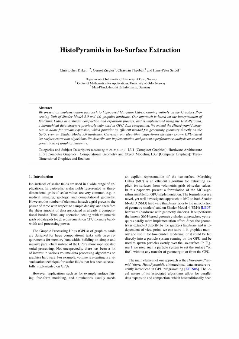
AbstractWe present an implementation approach to high-speed Marching Cubes, running entirely on the Graphics Pro-cessing Unit of Shader Model 3.0 and 4.0 graphics hardware. Our approach is based on the interpretation ofMarching Cubes as a stream compaction and expansion process, and is implemented using the HistoPyramid,a hierarchical data structure previously only used in GPU data compaction. We extend the HistoPyramid struc-ture to allow for stream expansion, which provides an efficient method for generating geometry directly on theGPU, even on Shader Model 3.0 hardware. Currently, our algorithm outperforms all other known GPU-basediso-surface extraction algorithms. We describe our implementation and present a performance analysis on severalgenerations of graphics hardware.

Categories and Subject Descriptors (according to ACM CCS): I.3.1 [Computer Graphics]: Hardware ArchitectureI.3.5 [Computer Graphics]: Computational Geometry and Object Modeling I.3.7 [Computer Graphics]: Three-Dimensional Graphics and Realism

1. Introduction

Iso-surfaces of scalar fields are used in a wide range of ap-plications. In particular, scalar fields represented as three-dimensional grids of scalar values are very common, e.g. inmedical imaging, geology, and computational geometry.However, the number of elements in such a grid grows to thepower of three with respect to sample density, and thereforethe sheer amount of data associated is already a computa-tional burden. Thus, any operation dealing with volumetricgrids of data puts tough requirements on CPU memory band-width and processing power.

The Graphic Processing Units (GPUs) of graphics cardsare designed for huge computational tasks with large re-quirements for memory bandwidth, building on simple andmassive parallelism instead of the CPU’s more sophisticatedserial processing. Not unexpectedly, there has been a lotof interest in various volume-data processing algorithms ongraphics hardware. For example, volume ray-casting is a vi-sualization technique for scalar fields that has been success-fully implemented on GPUs.

However, applications such as for example surface fair-ing, free-form modeling, and simulations usually needs

an explicit representation of the iso-surface. MarchingCubes (MC) is an efficient algorithm for extracting ex-plicit iso-surfaces from volumetric grids of scalar values.In this paper we present a formulation of the MC algo-rithm suitable for GPU implementation. The formulation is anovel, yet well-investigated approach to MC on both ShaderModel 3 (SM3) hardware (hardware prior to the introductionof geometry shaders) and on Shader Model 4 (SM4) [LB07]hardware (hardware with geometry shaders). It outperformsthe known SM4-based geometry-shader approaches, yet re-quires hardly more implementation effort. Since the geome-try is extracted directly by the graphics hardware and is in-dependent of view-point, we can store it in graphics mem-ory and use it for low-burden rendering, or it could be feddirectly into a particle system running on the GPU and beused to spawn particles evenly over the iso-surface. In Fig-ure 1 we used such a particle system to set the surface “onfire”, without any transfer of geometry to or from the CPU.

The main element of our approach is the Histogram Pyra-mid (short: HistoPyramid), a hierarchical data structure re-cently introduced in GPU programming [ZTTS06]. The lo-cal nature of its associated algorithms allow for paralleldata expansion and compaction, which has traditionally been

2 C. Dyken & G. Ziegler & C. Theobalt & H.-P. Seidel / HistoPyramids in Iso-Surface Extraction

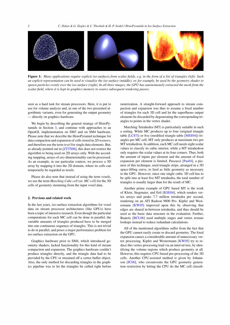
Figure 1: Many applications require explicit iso-surfaces from scalar fields, e.g. in the form of a list of triangles (left). Suchan explicit representation can be used to visualize the iso-surface (middle), or, for example, be used by the geometry shader tospawn particles evenly over the iso-surface (right). In all three images, the GPU has autonomously extracted the mesh from thescalar field, where it is kept in graphics memory to source subsequent rendering passes.

seen as a hard task for stream processors. Here, it is put touse for volume analysis and, in one of the two presented al-gorithmic variants, even for generating the output geometry— directly on graphics hardware.

We begin by describing the general strategy of HistoPy-ramids in Section 3, and continue with approaches to anOpenGL implementation on SM3 and on SM4 hardware.Please note that we describe the HistoPyramid technique fordata compaction and expansion of cells stored in 2D textures,and therefore use the term texel for single data elements. But,as already pointed out in [ZTTS06], this does not restrict thealgorithm to being used on 2D arrays only. With the accord-ing mapping, arrays of any dimensionality can be processed.As an example, in our particular context, we process a 3Darray by mapping it into the 2D domain, where its cells cantemporarily be regarded as texels.

Please do also note that instead of using the term voxels,we use the term Marching Cube cell (or: MC cell) for the 3Dcells of geometry stemming from the input voxel data.

2. Previous and related work

In the last years, iso-surface extraction algorithms for voxeldata on stream processor architectures (like GPUs) havebeen a topic of intensive research. Even though the particularcomputations for each MC cell can be done in parallel, thevariable amounts of triangles produced have to be mergedinto one continuous sequence of triangles. This is not trivialto do in parallel, and poses a major performance problem foriso-surface extraction on the GPU.

Graphics hardware prior to SM4, which introduced ge-ometry shaders, lacked functionality for this kind of streamcompaction and expansion. The graphics hardware couldn’tproduce triangles directly, and the triangle data had to beprovided by the CPU or streamed off a vertex buffer object.Also, the only method for discarding triangles in the graph-ics pipeline was to let the triangles be culled right before

rasterization. A straight-forward approach to stream com-paction and expansion was thus to assume a fixed numberof triangles for each 3D cell and let the superfluous outputelements be discarded by degenerating the corresponding tri-angles to points in the vertex shader.

Marching Tetrahedra (MT) is particularly suitable in sucha setting. While MC produces up to four (original triangletable [LC87]) or five (modified triangle table [MSS94]) tri-angles per MC cell, MT only produces at maximum two perMT tetrahedron. In addition, each MC cell needs eight scalarvalues to classify its cubic interior, while a MT tetrahedrononly requires the scalar values at its four corners. Thus, boththe amount of inputs per element and the amount of fixedexpansion per element is limited. Pascucci [Pas04], a pio-neer of this technique, used triangle strips, arranged in a 3Dspace-filling curve, to feed as little geometry as necessaryto the GPU. However, since one single cubic 3D cell has tobe split into at least five MT tetrahedra, the total number oftriangles is usually larger than for the result of MC.

Another prime example of GPU based MT is the workof Klein, Stegmaier, and Ertl [KSE04], which renders ver-tex arrays and peaks 7.7 million tetrahedra per second,rendering on an ATI Radeon 9800 Pro. Kipfer and West-ermann [KW05] improved upon this by observing thatedges are shared in-between tetrahedra, and thus should beused as the basic data structure in the evaluation. Further,Buatois [BCL06] used multiple stages and vertex texturelookups instead to reduce redundant calculations.

All of the mentioned algorithms suffer from the fact thatthe GPU cannot easily create or discard geometry. The fixedexpansion causes a considerable amount of unnecessary ver-tex processing. Kipfer and Westermann [KW05] try to re-duce this vertex processing load via an interval tree, by iden-tifying the volume regions which produce geometry at all.However, this requires CPU-based pre-processing of the 3Dcells. Another CPU-assisted method is given by Johann-son [JC06], who circumvents the GPU geometry genera-tion restriction by letting the CPU do the MC cell classifi-

C. Dyken & G. Ziegler & C. Theobalt & H.-P. Seidel / HistoPyramids in Iso-Surface Extraction 3

cation and only feeds the GPU with an MC cell if it actuallyproduces geometry. But Johannson also notes that this pre-processing on the CPU limits the speed of the algorithm.

Another drawback of these approaches is that none of thenamed algorithms is capable of creating a compact list ofthe iso-surface triangle mesh in GPU memory. Thus, part ofor the whole of the algorithm has to be run each time theresulting triangle mesh is rendered. Also, it is difficult to usethe set of triangles as input to other computations.

A first solution for GPU-based stream compaction isgiven in [Hor05]. It first uses a prefix sum method to gen-erate the correct output indices for each input element. Af-terwards, for each output element in the compacted out-put, it gathers the corresponding input element via a bi-nary search, ignoring unnecessary elements in the process.Unfortunately, their approach has a complexity of n log(n),and does not perform well on large datasets. Prefix Sum(Scan) [Har07] improved on this, and provides an efficientimplementation in CUDA. During a pyramid-like up-sweepand down-sweep phase, it creates, in parallel, a table thatassociates each input element with an offset in the out-put stream, at considerably reduced algorithmic complexity.Then, using this table and GPU scattering, it can directlyplace each relevant input element in the output list, while itignores the irrelevant elements.

Another approach to data compaction is provided byZiegler et.al. [ZTTS06] with the introduction of HistoPy-ramids, running entirely on the GPU of SM3 hardware. Asdemonstration, the algorithm is used to extract a compact se-quence of points from volumetric data. Despite a more com-plicated gather process for the output elements, the HistoPy-ramid is surprisingly fast when a considerable amount of in-put elements shall be discarded. In [DRS07], Dyken et.al.use this HistoPyramid for creating a compact list of silhou-ette edges, and can thus reduce the amount of data trans-ferred from GPU to CPU. The result is a silhouette detectionalgorithm faster than any CPU implementation for mesheslarger than a few thousand triangles.

The introduction of SM4 hardware provided data com-paction and expansion on the hardware level. The geometryshader, a new programmable stage in the graphics pipeline,has the ability to create and discard geometry on the fly.Uralsky [Ura06] present how MT can be implemented us-ing geometry shaders, with an implementation given in theNVidia OpenGL SDK-10. We have benchmarked our ap-proach against this implementation in Section 5. Anotherfeature of SM4, the transform feedback buffers, provide asimple method for tapping into the pipeline before rasteri-zation starts, and to record all the primitives submitted. Incombination, these two new features can also create a com-pact sequence of triangles in GPU memory.

1 0 0 0

0 2 0 1

1 0 1 0

1 1 0 1

Base level

3 1

3 2

Level 1

9

Level 2

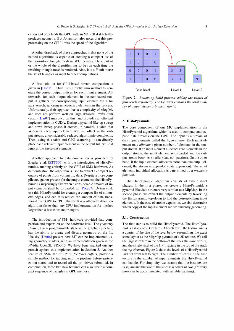
Figure 2: Bottom-up build process, adding the values offour texels repeatedly. The top texel contains the total num-ber of output elements in the pyramid.

3. HistoPyramids

The core component of our MC implementation is theHistoPyramid algorithm, which is used to compact and ex-pand data streams on the GPU. The input is a stream ofdata input elements called the input stream. Each input el-ement may allocate a given number of elements in the out-put stream. If an input element allocates zero elements in theoutput stream, the input element is discarded and the out-put stream becomes smaller (data compaction). On the otherhand, if the input element allocates more than one output el-ement, the stream is expanded (data expansion). The inputelements individual allocation is determined by a predicatefunction.

The HistoPyramid algorithm consists of two distinctphases. In the first phase, we create a HistoPyramid, apyramid-like data structure very similar to a MipMap. In thesecond phase, we extract the output elements by traversingthe HistoPyramid top-down to find the corresponding inputelements. In the case of stream expansion, we also determinewhich copy of the input element we are currently generating.

3.1. Construction

The first step is to build the HistoPyramid. The HistoPyra-mid is a stack of 2D textures. At each level, the texture size isa quarter of the size of the level below, resembling the exactsame layout as the MipMap pyramid of a 2D texture. We callthe largest texture in the bottom of the stack the base texture,and the single texel of the 1×1 texture in the top of the stackthe top element. Figure 2 show the levels of a HistoPyramidlaid out from left to right. The number of texels in the basetexture is the number of input elements the HistoPyramidcan handle. For simplicity, we assume that the base textureis square and the size of the sides is a power of two (arbitrarysizes can be accommodated with suitable padding).

4 C. Dyken & G. Ziegler & C. Theobalt & H.-P. Seidel / HistoPyramids in Iso-Surface Extraction

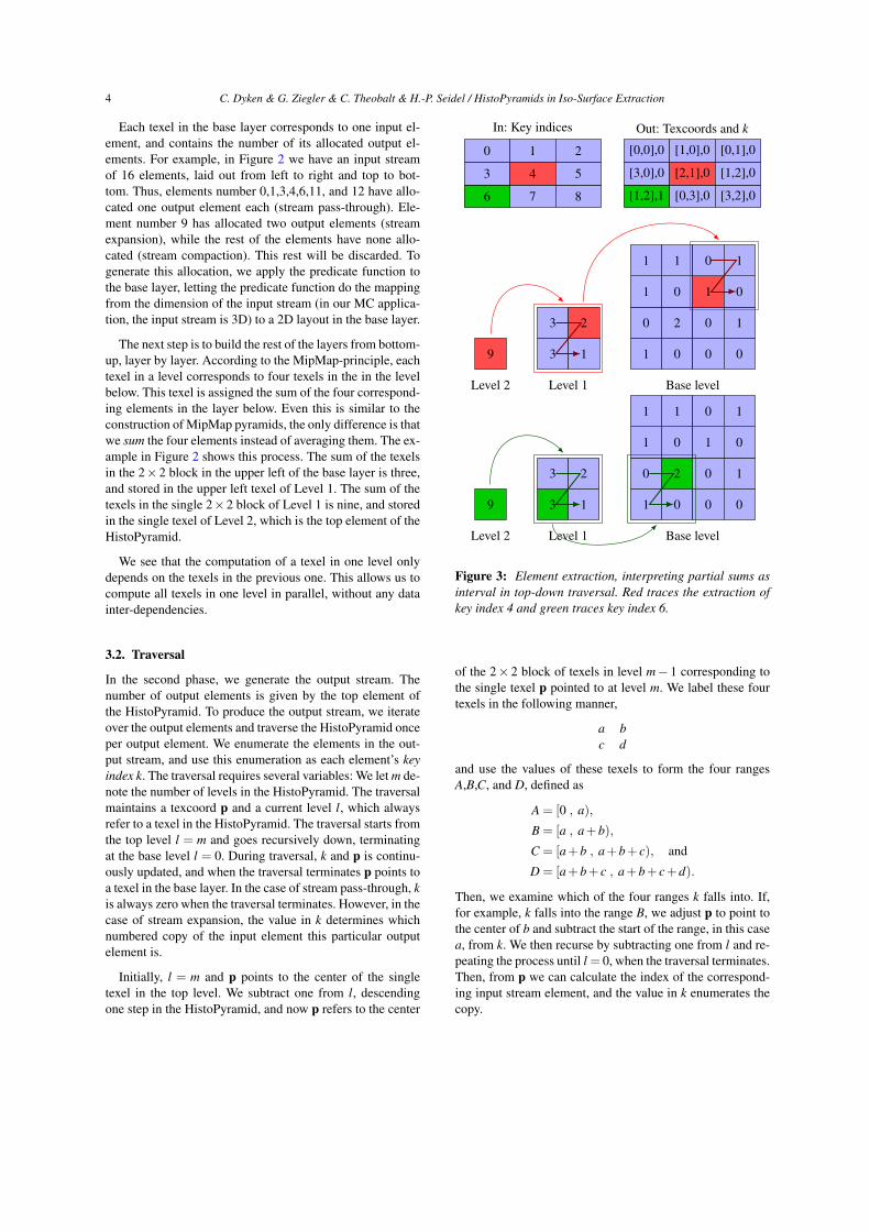
Each texel in the base layer corresponds to one input el-ement, and contains the number of its allocated output el-ements. For example, in Figure 2 we have an input streamof 16 elements, laid out from left to right and top to bot-tom. Thus, elements number 0,1,3,4,6,11, and 12 have allo-cated one output element each (stream pass-through). Ele-ment number 9 has allocated two output elements (streamexpansion), while the rest of the elements have none allo-cated (stream compaction). This rest will be discarded. Togenerate this allocation, we apply the predicate function tothe base layer, letting the predicate function do the mappingfrom the dimension of the input stream (in our MC applica-tion, the input stream is 3D) to a 2D layout in the base layer.

The next step is to build the rest of the layers from bottom-up, layer by layer. According to the MipMap-principle, eachtexel in a level corresponds to four texels in the in the levelbelow. This texel is assigned the sum of the four correspond-ing elements in the layer below. Even this is similar to theconstruction of MipMap pyramids, the only difference is thatwe sum the four elements instead of averaging them. The ex-ample in Figure 2 shows this process. The sum of the texelsin the 2×2 block in the upper left of the base layer is three,and stored in the upper left texel of Level 1. The sum of thetexels in the single 2×2 block of Level 1 is nine, and storedin the single texel of Level 2, which is the top element of theHistoPyramid.

We see that the computation of a texel in one level onlydepends on the texels in the previous one. This allows us tocompute all texels in one level in parallel, without any datainter-dependencies.

3.2. Traversal

In the second phase, we generate the output stream. Thenumber of output elements is given by the top element ofthe HistoPyramid. To produce the output stream, we iterateover the output elements and traverse the HistoPyramid onceper output element. We enumerate the elements in the out-put stream, and use this enumeration as each element’s keyindex k. The traversal requires several variables: We let m de-note the number of levels in the HistoPyramid. The traversalmaintains a texcoord p and a current level l, which alwaysrefer to a texel in the HistoPyramid. The traversal starts fromthe top level l = m and goes recursively down, terminatingat the base level l = 0. During traversal, k and p is continu-ously updated, and when the traversal terminates p points toa texel in the base layer. In the case of stream pass-through, kis always zero when the traversal terminates. However, in thecase of stream expansion, the value in k determines whichnumbered copy of the input element this particular outputelement is.

Initially, l = m and p points to the center of the singletexel in the top level. We subtract one from l, descendingone step in the HistoPyramid, and now p refers to the center

In: Key indices

6 7 8

3 4 5

0 1 2

Out: Texcoords and k

[1,2],1 [0,3],0 [3,2],0

[3,0],0 [2,1],0 [1,2],0

[0,0],0 [1,0],0 [0,1],0

1 0 0 0

0 2 0 1

1 0 1 0

1 1 0 1

Base level

3 1

3 2

Level 1

9

Level 2

1 0 0 0

0 2 0 1

1 0 1 0

1 1 0 1

Base level

3 1

3 2

Level 1

9

Level 2

Figure 3: Element extraction, interpreting partial sums asinterval in top-down traversal. Red traces the extraction ofkey index 4 and green traces key index 6.

of the 2× 2 block of texels in level m− 1 corresponding tothe single texel p pointed to at level m. We label these fourtexels in the following manner,

a bc d

and use the values of these texels to form the four rangesA,B,C, and D, defined as

A = [0 , a),

B = [a , a+b),

C = [a+b , a+b+ c), and

D = [a+b+ c , a+b+ c+d).

Then, we examine which of the four ranges k falls into. If,for example, k falls into the range B, we adjust p to point tothe center of b and subtract the start of the range, in this casea, from k. We then recurse by subtracting one from l and re-peating the process until l = 0, when the traversal terminates.Then, from p we can calculate the index of the correspond-ing input stream element, and the value in k enumerates thecopy.

C. Dyken & G. Ziegler & C. Theobalt & H.-P. Seidel / HistoPyramids in Iso-Surface Extraction 5

Figure 3 show two examples of HistoPyramid traversal.The first example, labeled red, is of the key index k = 4, isa case of stream copy. We start at level 2 and descend tolevel 1. The four texels at level 1 form the ranges

A = [0 , 3), B = [3 , 5), C = [5 , 8), D = [8 , 9).

We see that k is in the range B. Thus, we adjust the texcoordto point to the upper left texel and subtract 3 from k, whichleaves k = 1. Then, we descend again to the base level. Thefour texels in the base level corresponding to the upper lefttexel of level 1 form the ranges

A = [0 , 0), B = [0 , 1), C = [1 , 2), D = [2 , 2).

The ranges A and D are empty. Here, k = 1 falls into B, andwe adjust p and k accordingly. Since we’re at the base level,the traversal terminates, p = [2,1] and k = 0.

The second example of Figure 3, labeled green, is a caseof stream expansion. Here the key index k = 6. We begin atthe top of the HistoPyramid and descend to level 2. Again,the four texels form the ranges

A = [0 , 3), B = [3 , 5), C = [5 , 8), D = [8 , 9),

And k falls into the range C. We adjust p to point to c andsubtract the start of range C from k, resulting in k = 1. De-scending, we inspect the four texels in the lower left cornerof the base layer, which form the four ranges

A = [0 , 0), B = [0 , 2), C = [2 , 3), D = [3 , 3),

Here, k falls into range B, and we adjust p and k accordingly.Since we’re at the base level, we terminate the traversal, andhave p = [1,2] and k = 1. This means that output element 6 isthe second output element (since k = 1) of the input elementcorresponding to the position [1,2] in the base texture.

The traversal only reads from the HistoPyramid and thereare no data dependencies between traversals. Therefore, theoutput elements can be extracted in any order, for example,at the same time in parallel.

3.3. Comments

The 2D texture layout of the HistoPyramid fits graphicshardware very well. It can intuitively be seen that in thedomain of normalized texcoord calculations, the texturefetches overlay with fetches from the layer below. This al-lows the 2D texture cache to assist HP traversal with mem-ory prefetches, and thus increase its performance.

At each descend during the traversal, we have to inspectthe values of four texels, which amounts to four texturefetches. However, since we always fetch 2×2 blocks, we canuse a four-channel texture and encode these four values as aRGBA value. This halves the size of all textures along bothdimensions, and lets us thus build four times larger HistoPy-ramids within the same texture size limits. In addition, sincewe quarter the number of texture fetches, and graphics hard-ware is quite efficient at fetching four-channel RGBA values,

a

c

(e, f )

(b, f )

( f ,h)

b

d

e f

g h

x

y

z

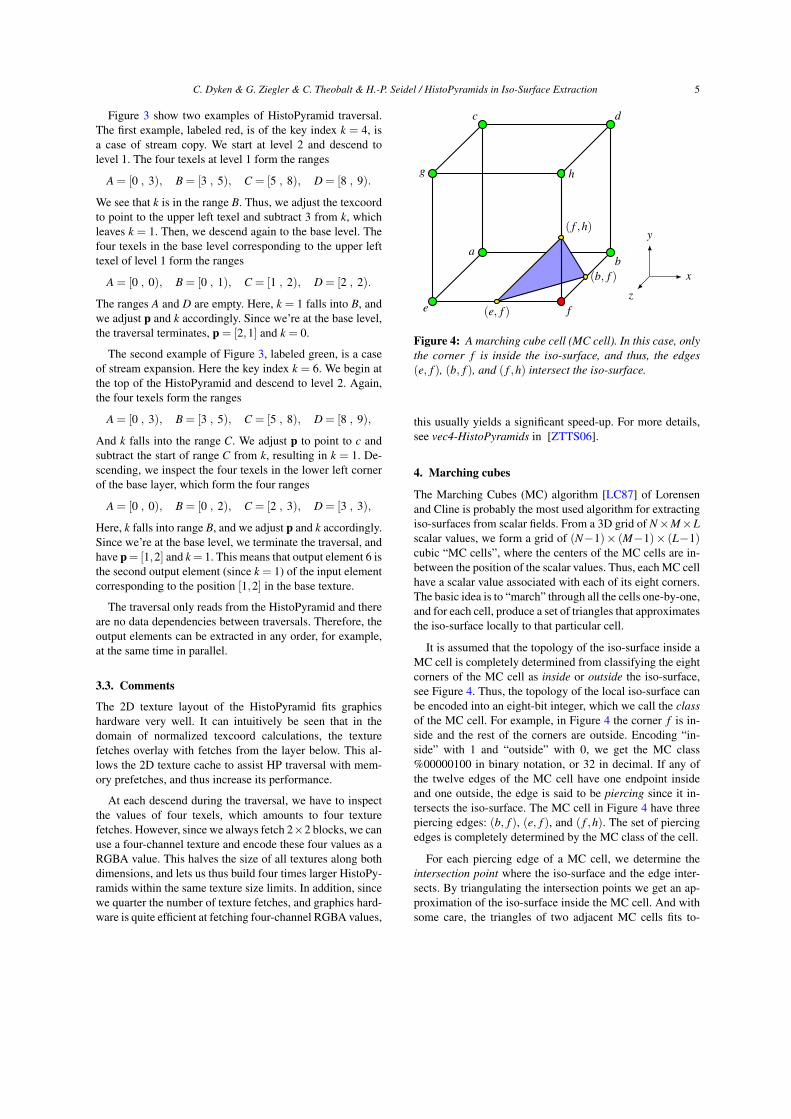
Figure 4: A marching cube cell (MC cell). In this case, onlythe corner f is inside the iso-surface, and thus, the edges(e, f ), (b, f ), and ( f ,h) intersect the iso-surface.

this usually yields a significant speed-up. For more details,see vec4-HistoPyramids in [ZTTS06].

4. Marching cubes

The Marching Cubes (MC) algorithm [LC87] of Lorensenand Cline is probably the most used algorithm for extractingiso-surfaces from scalar fields. From a 3D grid of N×M×Lscalar values, we form a grid of (N−1)× (M−1)× (L−1)cubic “MC cells”, where the centers of the MC cells are in-between the position of the scalar values. Thus, each MC cellhave a scalar value associated with each of its eight corners.The basic idea is to “march” through all the cells one-by-one,and for each cell, produce a set of triangles that approximatesthe iso-surface locally to that particular cell.

It is assumed that the topology of the iso-surface inside aMC cell is completely determined from classifying the eightcorners of the MC cell as inside or outside the iso-surface,see Figure 4. Thus, the topology of the local iso-surface canbe encoded into an eight-bit integer, which we call the classof the MC cell. For example, in Figure 4 the corner f is in-side and the rest of the corners are outside. Encoding “in-side” with 1 and “outside” with 0, we get the MC class%00000100 in binary notation, or 32 in decimal. If any ofthe twelve edges of the MC cell have one endpoint insideand one outside, the edge is said to be piercing since it in-tersects the iso-surface. The MC cell in Figure 4 have threepiercing edges: (b, f ), (e, f ), and ( f ,h). The set of piercingedges is completely determined by the MC class of the cell.

For each piercing edge of a MC cell, we determine theintersection point where the iso-surface and the edge inter-sects. By triangulating the intersection points we get an ap-proximation of the iso-surface inside the MC cell. And withsome care, the triangles of two adjacent MC cells fits to-

6 C. Dyken & G. Ziegler & C. Theobalt & H.-P. Seidel / HistoPyramids in Iso-Surface Extraction

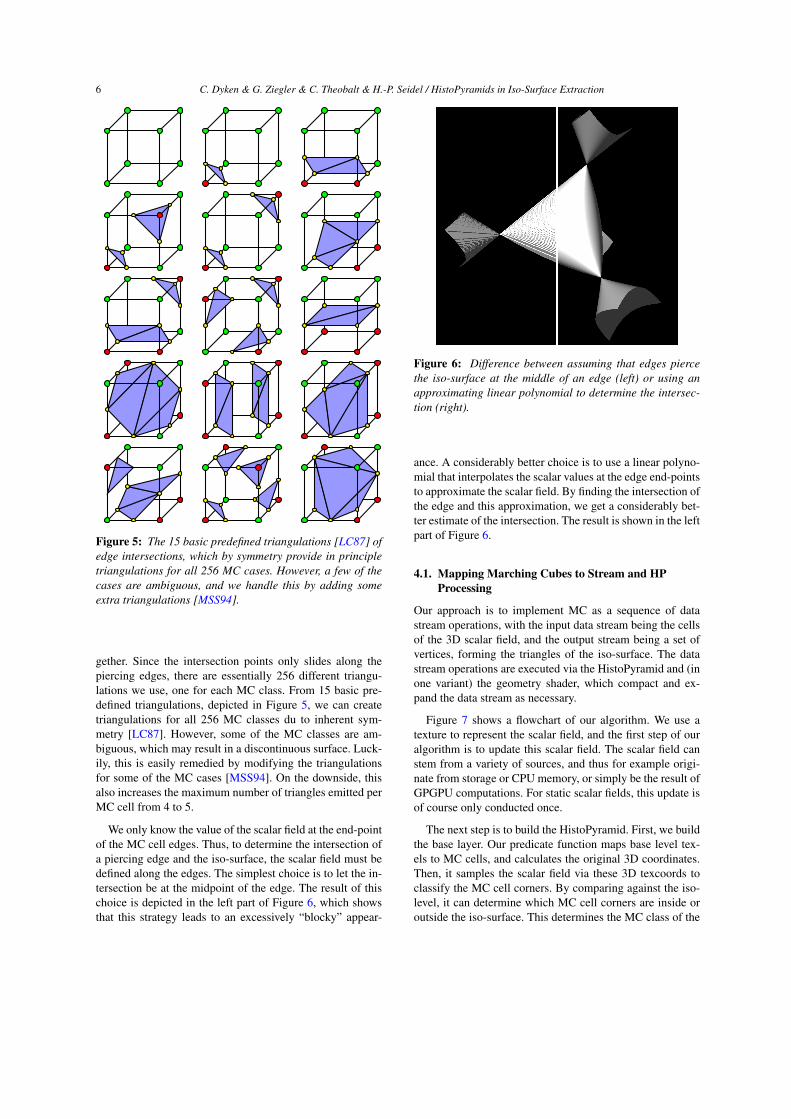
Figure 5: The 15 basic predefined triangulations [LC87] ofedge intersections, which by symmetry provide in principletriangulations for all 256 MC cases. However, a few of thecases are ambiguous, and we handle this by adding someextra triangulations [MSS94].

gether. Since the intersection points only slides along thepiercing edges, there are essentially 256 different triangu-lations we use, one for each MC class. From 15 basic pre-defined triangulations, depicted in Figure 5, we can createtriangulations for all 256 MC classes du to inherent sym-metry [LC87]. However, some of the MC classes are am-biguous, which may result in a discontinuous surface. Luck-ily, this is easily remedied by modifying the triangulationsfor some of the MC cases [MSS94]. On the downside, thisalso increases the maximum number of triangles emitted perMC cell from 4 to 5.

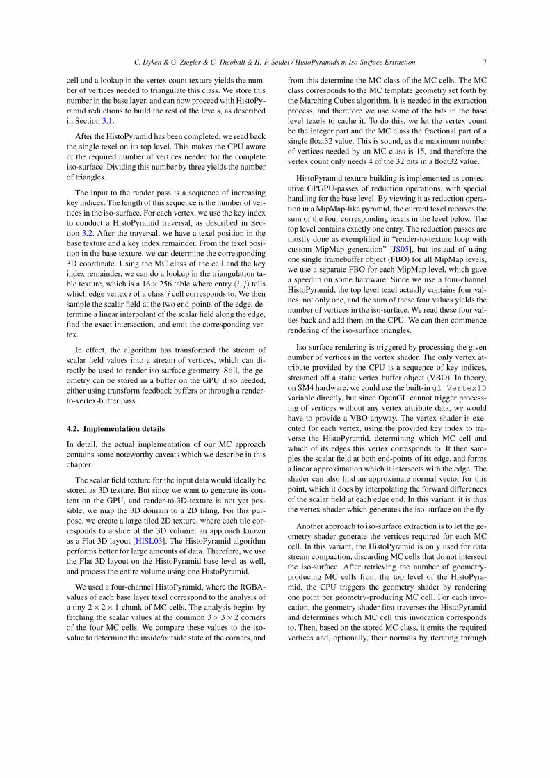
We only know the value of the scalar field at the end-pointof the MC cell edges. Thus, to determine the intersection ofa piercing edge and the iso-surface, the scalar field must bedefined along the edges. The simplest choice is to let the in-tersection be at the midpoint of the edge. The result of thischoice is depicted in the left part of Figure 6, which showsthat this strategy leads to an excessively “blocky” appear-

Figure 6: Difference between assuming that edges piercethe iso-surface at the middle of an edge (left) or using anapproximating linear polynomial to determine the intersec-tion (right).

ance. A considerably better choice is to use a linear polyno-mial that interpolates the scalar values at the edge end-pointsto approximate the scalar field. By finding the intersection ofthe edge and this approximation, we get a considerably bet-ter estimate of the intersection. The result is shown in the leftpart of Figure 6.

4.1. Mapping Marching Cubes to Stream and HPProcessing

Our approach is to implement MC as a sequence of datastream operations, with the input data stream being the cellsof the 3D scalar field, and the output stream being a set ofvertices, forming the triangles of the iso-surface. The datastream operations are executed via the HistoPyramid and (inone variant) the geometry shader, which compact and ex-pand the data stream as necessary.

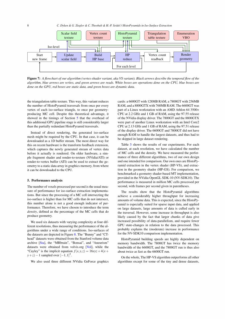
Figure 7 shows a flowchart of our algorithm. We use atexture to represent the scalar field, and the first step of ouralgorithm is to update this scalar field. The scalar field canstem from a variety of sources, and thus for example origi-nate from storage or CPU memory, or simply be the result ofGPGPU computations. For static scalar fields, this update isof course only conducted once.

The next step is to build the HistoPyramid. First, we buildthe base layer. Our predicate function maps base level tex-els to MC cells, and calculates the original 3D coordinates.Then, it samples the scalar field via these 3D texcoords toclassify the MC cell corners. By comparing against the iso-level, it can determine which MC cell corners are inside oroutside the iso-surface. This determines the MC class of the

C. Dyken & G. Ziegler & C. Theobalt & H.-P. Seidel / HistoPyramids in Iso-Surface Extraction 7

cell and a lookup in the vertex count texture yields the num-ber of vertices needed to triangulate this class. We store thisnumber in the base layer, and can now proceed with HistoPy-ramid reductions to build the rest of the levels, as describedin Section 3.1.

After the HistoPyramid has been completed, we read backthe single texel on its top level. This makes the CPU awareof the required number of vertices needed for the completeiso-surface. Dividing this number by three yields the numberof triangles.

The input to the render pass is a sequence of increasingkey indices. The length of this sequence is the number of ver-tices in the iso-surface. For each vertex, we use the key indexto conduct a HistoPyramid traversal, as described in Sec-tion 3.2. After the traversal, we have a texel position in thebase texture and a key index remainder. From the texel posi-tion in the base texture, we can determine the corresponding3D coordinate. Using the MC class of the cell and the keyindex remainder, we can do a lookup in the triangulation ta-ble texture, which is a 16×256 table where entry (i, j) tellswhich edge vertex i of a class j cell corresponds to. We thensample the scalar field at the two end-points of the edge, de-termine a linear interpolant of the scalar field along the edge,find the exact intersection, and emit the corresponding ver-tex.

In effect, the algorithm has transformed the stream ofscalar field values into a stream of vertices, which can di-rectly be used to render iso-surface geometry. Still, the ge-ometry can be stored in a buffer on the GPU if so needed,either using transform feedback buffers or through a render-to-vertex-buffer pass.

4.2. Implementation details

In detail, the actual implementation of our MC approachcontains some noteworthy caveats which we describe in thischapter.

The scalar field texture for the input data would ideally bestored as 3D texture. But since we want to generate its con-tent on the GPU, and render-to-3D-texture is not yet pos-sible, we map the 3D domain to a 2D tiling. For this pur-pose, we create a large tiled 2D texture, where each tile cor-responds to a slice of the 3D volume, an approach knownas a Flat 3D layout [HISL03]. The HistoPyramid algorithmperforms better for large amounts of data. Therefore, we usethe Flat 3D layout on the HistoPyramid base level as well,and process the entire volume using one HistoPyramid.

We used a four-channel HistoPyramid, where the RGBA-values of each base layer texel correspond to the analysis ofa tiny 2× 2× 1-chunk of MC cells. The analysis begins byfetching the scalar values at the common 3× 3× 2 cornersof the four MC cells. We compare these values to the iso-value to determine the inside/outside state of the corners, and

from this determine the MC class of the MC cells. The MCclass corresponds to the MC template geometry set forth bythe Marching Cubes algorithm. It is needed in the extractionprocess, and therefore we use some of the bits in the baselevel texels to cache it. To do this, we let the vertex countbe the integer part and the MC class the fractional part of asingle float32 value. This is sound, as the maximum numberof vertices needed by an MC class is 15, and therefore thevertex count only needs 4 of the 32 bits in a float32 value.

HistoPyramid texture building is implemented as consec-utive GPGPU-passes of reduction operations, with specialhandling for the base level. By viewing it as reduction opera-tion in a MipMap-like pyramid, the current texel receives thesum of the four corresponding texels in the level below. Thetop level contains exactly one entry. The reduction passes aremostly done as exemplified in “render-to-texture loop withcustom MipMap generation” [JS05], but instead of usingone single framebuffer object (FBO) for all MipMap levels,we use a separate FBO for each MipMap level, which gavea speedup on some hardware. Since we use a four-channelHistoPyramid, the top level texel actually contains four val-ues, not only one, and the sum of these four values yields thenumber of vertices in the iso-surface. We read these four val-ues back and add them on the CPU. We can then commencerendering of the iso-surface triangles.

Iso-surface rendering is triggered by processing the givennumber of vertices in the vertex shader. The only vertex at-tribute provided by the CPU is a sequence of key indices,streamed off a static vertex buffer object (VBO). In theory,on SM4 hardware, we could use the built-in gl_VertexIDvariable directly, but since OpenGL cannot trigger process-ing of vertices without any vertex attribute data, we wouldhave to provide a VBO anyway. The vertex shader is exe-cuted for each vertex, using the provided key index to tra-verse the HistoPyramid, determining which MC cell andwhich of its edges this vertex corresponds to. It then sam-ples the scalar field at both end-points of its edge, and formsa linear approximation which it intersects with the edge. Theshader can also find an approximate normal vector for thispoint, which it does by interpolating the forward differencesof the scalar field at each edge end. In this variant, it is thusthe vertex-shader which generates the iso-surface on the fly.

Another approach to iso-surface extraction is to let the ge-ometry shader generate the vertices required for each MCcell. In this variant, the HistoPyramid is only used for datastream compaction, discarding MC cells that do not intersectthe iso-surface. After retrieving the number of geometry-producing MC cells from the top level of the HistoPyra-mid, the CPU triggers the geometry shader by renderingone point per geometry-producing MC cell. For each invo-cation, the geometry shader first traverses the HistoPyramidand determines which MC cell this invocation correspondsto. Then, based on the stored MC class, it emits the requiredvertices and, optionally, their normals by iterating through

8 C. Dyken & G. Ziegler & C. Theobalt & H.-P. Seidel / HistoPyramids in Iso-Surface Extraction

Scalar fieldtexture

Vertex counttexture

HistoPyramidtexture

Triangulationtable texture

EnumerationVBO

Startnew frame

Updatescalar field

BuildHP base

HPreduce

Vertex countreadback

Rendergeometry

Iso-level

For each level

Figure 7: A flowchart of our algorithm (vertex-shader variant, aka VS variant). Black arrows describe the temporal flow of thealgorithm, blue arrows are writes, and green arrows are reads. White boxes are operations done on the CPU, blue boxes aredone on the GPU, red boxes are static data, and green boxes are dynamic data.

the triangulation table texture. This way, this variant reducesthe number of HistoPyramid traversals from once per everyvertex of each iso-surface triangle, to once per geometry-producing MC cell. Despite this theoretical advantage, itshowed in the timings of Section 5 that the overhead ofthis additional GPU pipeline stage is still considerably largerthan the partially redundant HistoPyramid traversals.

Instead of direct rendering, the generated iso-surfacemesh might be required by the CPU. In that case, it can bedownloaded as a 1D buffer stream. The most direct way forthis on recent hardware is the transform feedback extension,which captures the newly generated stream of vertex databefore it actually is rendered. On older hardware, a sim-ple fragment shader and render-to-texture (NVidia/ATI) orrender-to-vertex buffer (ATI) can be used to extract the ge-ometry to a static data array in graphics memory, from whereit can be downloaded to the CPU.

5. Performance analysis

The number of voxels processed per second is the usual mea-sure of performance for iso-surface extraction implementa-tions. But since the processing of a MC cell intersecting theiso-surface is higher than for MC cells that do not intersect,this number alone is not a good enough indicator of per-formance. Therefore, we have chosen to introduce the termdensity, defined as the percentage of the MC cells that doproduce geometry.

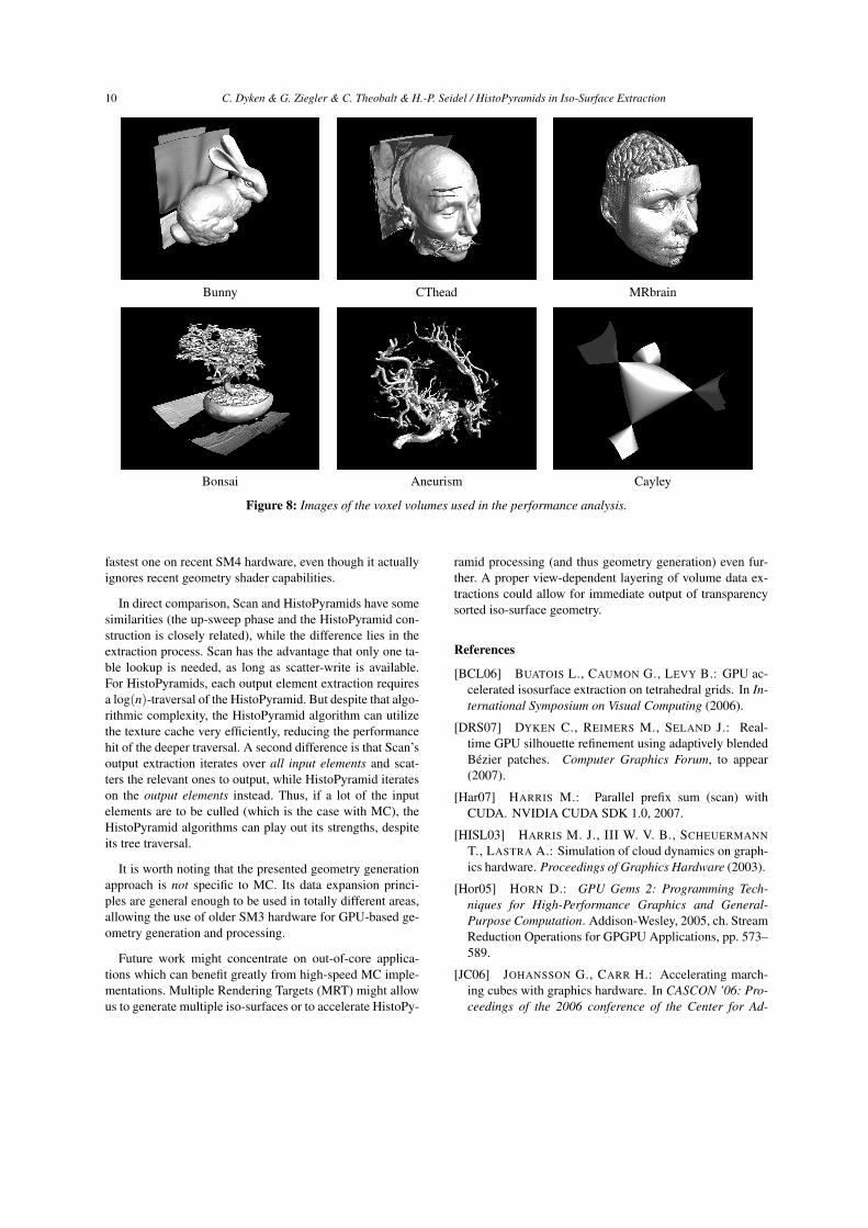
We used six datasets with varying complexity at four dif-ferent resolutions, thus measuring the performance of the al-gorithms under a wide range of conditions. Iso-surfaces ofthe datasets are depicted in Figure 8. The “Bunny” and “CT-head” datasets were obtained from the Stanford volume dataarchive [Sta], the “MRbrain”, “Bonsai”, and “Aneurism”datasets were obtained from volvis.org [Vol], while the“Cayley” is the implicit equation f (x,y,z) = 16xyz + 4(x +y+ z)−1 sampled over [−1,1]3.

We also used three different NVidia GeForce graphics

cards: a 6600GT with 128MB RAM, a 7800GT with 256MBRAM, and a 8800GTX with 768MB RAM. The 6600GT waspart of a Linux workstation with an AMD Athlon 64 3500+CPU at 2.2 GHz and 1 GB of RAM, using the 97.55 releaseof the NVidia display driver. The 7800GT and the 8800GTXwere part of another Linux workstation with an Intel Core2CPU at 2.13 GHz and 1 GB of RAM, using the 97.51 releaseof the display driver. The 6600GT and 7800GT did not haveenough RAM to handle the largest datasets, and thus had tobe skipped in large dataset rendering.

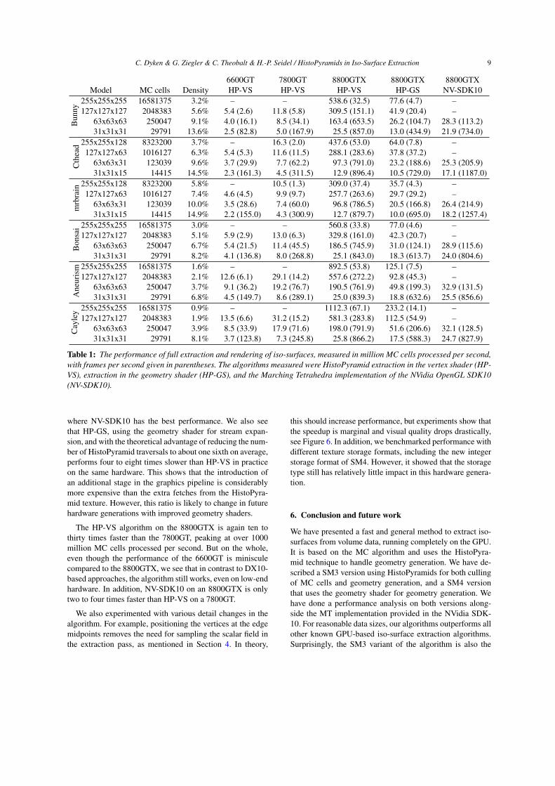
Table 5 shows the results of our experiments. For eachdataset, at each resolution, we have calculated the numberof MC cells and the density. We have measured the perfor-mance of three different algorithms, two of our own designand one intended for comparison. Our own ones are HistoPy-ramid extraction in the vertex shader (HP-VS), and extrac-tion in the geometry shader (HP-GS). For comparison, webenchmarked a geometry shader-based MT implementation,provided in the NVidia OpenGL SDK-10 (NV-SDK10). Theperformance is measured in million MC cells processed persecond, with frames per second given in parentheses.

The results show that the HistoPyramid algorithmsachieve a considerably higher throughput for increasingamounts of volume data. This is expected, since the HistoPy-ramid is especially suited for sparse input data, and appliedon large datasets, large amounts of data is culled early inthe traversal. However, some increase in throughput is alsolikely caused by the fact that larger chunks of data giveincreased possibility of data-parallelism, and require fewerGPU state-changes in relation to the data processed. Thisprobably explains the (moderate) increase in performancefor the NV-SDK10 comparison implementation.

HistoPyramid building speeds are highly dependent onmemory bandwidth. The 7800GT has twice the memorybandwidth of the 6600GT, and the 7800GT run is thus alsoabout twice as fast as the 6600GT run.

On the whole, The HP-VS algorithm outperforms all otheralgorithms except for some of the tiny and dense datasets,

C. Dyken & G. Ziegler & C. Theobalt & H.-P. Seidel / HistoPyramids in Iso-Surface Extraction 9

6600GT 7800GT 8800GTX 8800GTX 8800GTXModel MC cells Density HP-VS HP-VS HP-VS HP-GS NV-SDK10

Bun

ny

255x255x255 16581375 3.2% – – 538.6 (32.5) 77.6 (4.7) –127x127x127 2048383 5.6% 5.4 (2.6) 11.8 (5.8) 309.5 (151.1) 41.9 (20.4) –

63x63x63 250047 9.1% 4.0 (16.1) 8.5 (34.1) 163.4 (653.5) 26.2 (104.7) 28.3 (113.2)31x31x31 29791 13.6% 2.5 (82.8) 5.0 (167.9) 25.5 (857.0) 13.0 (434.9) 21.9 (734.0)

Cth

ead 255x255x128 8323200 3.7% – 16.3 (2.0) 437.6 (53.0) 64.0 (7.8) –

127x127x63 1016127 6.3% 5.4 (5.3) 11.6 (11.5) 288.1 (283.6) 37.8 (37.2) –63x63x31 123039 9.6% 3.7 (29.9) 7.7 (62.2) 97.3 (791.0) 23.2 (188.6) 25.3 (205.9)31x31x15 14415 14.5% 2.3 (161.3) 4.5 (311.5) 12.9 (896.4) 10.5 (729.0) 17.1 (1187.0)

mrb

rain 255x255x128 8323200 5.8% – 10.5 (1.3) 309.0 (37.4) 35.7 (4.3) –

127x127x63 1016127 7.4% 4.6 (4.5) 9.9 (9.7) 257.7 (263.6) 29.7 (29.2) –63x63x31 123039 10.0% 3.5 (28.6) 7.4 (60.0) 96.8 (786.5) 20.5 (166.8) 26.4 (214.9)31x31x15 14415 14.9% 2.2 (155.0) 4.3 (300.9) 12.7 (879.7) 10.0 (695.0) 18.2 (1257.4)

Bon

sai 255x255x255 16581375 3.0% – – 560.8 (33.8) 77.0 (4.6) –

127x127x127 2048383 5.1% 5.9 (2.9) 13.0 (6.3) 329.8 (161.0) 42.3 (20.7) –63x63x63 250047 6.7% 5.4 (21.5) 11.4 (45.5) 186.5 (745.9) 31.0 (124.1) 28.9 (115.6)31x31x31 29791 8.2% 4.1 (136.8) 8.0 (268.8) 25.1 (843.0) 18.3 (613.7) 24.0 (804.6)

Ane

uris

m 255x255x255 16581375 1.6% – – 892.5 (53.8) 125.1 (7.5) –127x127x127 2048383 2.1% 12.6 (6.1) 29.1 (14.2) 557.6 (272.2) 92.8 (45.3) –

63x63x63 250047 3.7% 9.1 (36.2) 19.2 (76.7) 190.5 (761.9) 49.8 (199.3) 32.9 (131.5)31x31x31 29791 6.8% 4.5 (149.7) 8.6 (289.1) 25.0 (839.3) 18.8 (632.6) 25.5 (856.6)

Cay

ley 255x255x255 16581375 0.9% – – 1112.3 (67.1) 233.2 (14.1) –

127x127x127 2048383 1.9% 13.5 (6.6) 31.2 (15.2) 581.3 (283.8) 112.5 (54.9) –63x63x63 250047 3.9% 8.5 (33.9) 17.9 (71.6) 198.0 (791.9) 51.6 (206.6) 32.1 (128.5)31x31x31 29791 8.1% 3.7 (123.8) 7.3 (245.8) 25.8 (866.2) 17.5 (588.3) 24.7 (827.9)

Table 1: The performance of full extraction and rendering of iso-surfaces, measured in million MC cells processed per second,with frames per second given in parentheses. The algorithms measured were HistoPyramid extraction in the vertex shader (HP-VS), extraction in the geometry shader (HP-GS), and the Marching Tetrahedra implementation of the NVidia OpenGL SDK10(NV-SDK10).

where NV-SDK10 has the best performance. We also seethat HP-GS, using the geometry shader for stream expan-sion, and with the theoretical advantage of reducing the num-ber of HistoPyramid traversals to about one sixth on average,performs four to eight times slower than HP-VS in practiceon the same hardware. This shows that the introduction ofan additional stage in the graphics pipeline is considerablymore expensive than the extra fetches from the HistoPyra-mid texture. However, this ratio is likely to change in futurehardware generations with improved geometry shaders.

The HP-VS algorithm on the 8800GTX is again ten tothirty times faster than the 7800GT, peaking at over 1000million MC cells processed per second. But on the whole,even though the performance of the 6600GT is minisculecompared to the 8800GTX, we see that in contrast to DX10-based approaches, the algorithm still works, even on low-endhardware. In addition, NV-SDK10 on an 8800GTX is onlytwo to four times faster than HP-VS on a 7800GT.

We also experimented with various detail changes in thealgorithm. For example, positioning the vertices at the edgemidpoints removes the need for sampling the scalar field inthe extraction pass, as mentioned in Section 4. In theory,

this should increase performance, but experiments show thatthe speedup is marginal and visual quality drops drastically,see Figure 6. In addition, we benchmarked performance withdifferent texture storage formats, including the new integerstorage format of SM4. However, it showed that the storagetype still has relatively little impact in this hardware genera-tion.

6. Conclusion and future work

We have presented a fast and general method to extract iso-surfaces from volume data, running completely on the GPU.It is based on the MC algorithm and uses the HistoPyra-mid technique to handle geometry generation. We have de-scribed a SM3 version using HistoPyramids for both cullingof MC cells and geometry generation, and a SM4 versionthat uses the geometry shader for geometry generation. Wehave done a performance analysis on both versions along-side the MT implementation provided in the NVidia SDK-10. For reasonable data sizes, our algorithms outperforms allother known GPU-based iso-surface extraction algorithms.Surprisingly, the SM3 variant of the algorithm is also the

10 C. Dyken & G. Ziegler & C. Theobalt & H.-P. Seidel / HistoPyramids in Iso-Surface Extraction

Bunny CThead MRbrain

Bonsai Aneurism Cayley

Figure 8: Images of the voxel volumes used in the performance analysis.

fastest one on recent SM4 hardware, even though it actuallyignores recent geometry shader capabilities.

In direct comparison, Scan and HistoPyramids have somesimilarities (the up-sweep phase and the HistoPyramid con-struction is closely related), while the difference lies in theextraction process. Scan has the advantage that only one ta-ble lookup is needed, as long as scatter-write is available.For HistoPyramids, each output element extraction requiresa log(n)-traversal of the HistoPyramid. But despite that algo-rithmic complexity, the HistoPyramid algorithm can utilizethe texture cache very efficiently, reducing the performancehit of the deeper traversal. A second difference is that Scan’soutput extraction iterates over all input elements and scat-ters the relevant ones to output, while HistoPyramid iterateson the output elements instead. Thus, if a lot of the inputelements are to be culled (which is the case with MC), theHistoPyramid algorithms can play out its strengths, despiteits tree traversal.

It is worth noting that the presented geometry generationapproach is not specific to MC. Its data expansion princi-ples are general enough to be used in totally different areas,allowing the use of older SM3 hardware for GPU-based ge-ometry generation and processing.

Future work might concentrate on out-of-core applica-tions which can benefit greatly from high-speed MC imple-mentations. Multiple Rendering Targets (MRT) might allowus to generate multiple iso-surfaces or to accelerate HistoPy-

ramid processing (and thus geometry generation) even fur-ther. A proper view-dependent layering of volume data ex-tractions could allow for immediate output of transparencysorted iso-surface geometry.

References

[BCL06] BUATOIS L., CAUMON G., LEVY B.: GPU ac-celerated isosurface extraction on tetrahedral grids. In In-ternational Symposium on Visual Computing (2006).

[DRS07] DYKEN C., REIMERS M., SELAND J.: Real-time GPU silhouette refinement using adaptively blendedBézier patches. Computer Graphics Forum, to appear(2007).

[Har07] HARRIS M.: Parallel prefix sum (scan) withCUDA. NVIDIA CUDA SDK 1.0, 2007.

[HISL03] HARRIS M. J., III W. V. B., SCHEUERMANN

T., LASTRA A.: Simulation of cloud dynamics on graph-ics hardware. Proceedings of Graphics Hardware (2003).

[Hor05] HORN D.: GPU Gems 2: Programming Tech-niques for High-Performance Graphics and General-Purpose Computation. Addison-Wesley, 2005, ch. StreamReduction Operations for GPGPU Applications, pp. 573–589.

[JC06] JOHANSSON G., CARR H.: Accelerating march-ing cubes with graphics hardware. In CASCON ’06: Pro-ceedings of the 2006 conference of the Center for Ad-

C. Dyken & G. Ziegler & C. Theobalt & H.-P. Seidel / HistoPyramids in Iso-Surface Extraction 11

vanced Studies on Collaborative research (2006), ACMPress.

[JS05] JULIANO J., SANDMEL J.: GL_EXT_frame-buffer_object. OpenGL extension registry, 2005.

[KSE04] KLEIN T., STEGMAIER S., ERTL T.: Hardware-accelerated reconstruction of polygonal isosurface repre-sentations on unstructured grids. Pacific Graphics 2004Proceedings (2004).

[KW05] KIPFER P., WESTERMANN R.: GPU construc-tion and transparent rendering of iso-surface. In Pro-ceedings Vision, Modeling and Visualization 2005 (2005),Greiner G., Hornegger J., Niemann H., Stamminger M.,(Eds.), IOS Press, infix, pp. 241–248.

[LB07] LICHTENBELT B., BROWN P.: GL_EXT_gpu_shader4. OpenGL extension registry, 2007.

[LC87] LORENSEN W., CLINE H. E.: Marching cubes:A high resolution 3d surface construction algorithm.Computer Graphics (SIGGRAPH 87 Proceedings) 21, 4(1987), 163–170.

[MSS94] MONTANI C., SCATENI R., SCOPIGNO R.: Amodified look-up table for implicit disambiguation ofMarching Cubes. The Visual Computer 10 (1994), 353–355.

[Pas04] PASCUCCI V.: Isosurface computation made sim-ple: Hardware acceleration, adaptive refinement and tetra-hedral stripping. Joint Eurographics - IEEE TVCG Sym-posium on Visualization (2004), 292–300.

[Sta] The stanford volume data archive. http://graphics.stanford.edu/data/voldata/.

[Ura06] URALSKY Y.: DX10: Practical metaballs and im-plicit surfaces. GameDevelopers conference, 2006.

[Vol] Volvis volume dataset archive. http://www.volvis.org/.

[ZTTS06] ZIEGLER G., TEVS A., THEOBALT C., SEI-DEL H.-P.: GPU Point List Generation through His-togram Pyramids. Tech. Rep. MPI-I-2006-4-002, Max-Planck-Institut für Informatik, 2006.

Below you find a list of the most recent technical reports of the Max-Planck-Institut fur Informatik. Theyare available by anonymous ftp from ftp.mpi-sb.mpg.de under the directory pub/papers/reports. Mostof the reports are also accessible via WWW using the URL http://www.mpi-sb.mpg.de. If you have anyquestions concerning ftp or WWW access, please contact reports@mpi-sb.mpg.de. Paper copies (whichare not necessarily free of charge) can be ordered either by regular mail or by e-mail at the address below.

Max-Planck-Institut fur InformatikLibraryattn. Anja BeckerStuhlsatzenhausweg 8566123 SaarbruckenGERMANYe-mail: library@mpi-sb.mpg.de

MPI-I-2006-5-001 M. Bender, S. Michel, G. Weikum,P. Triantafilou

Overlap-Aware Global df Estimation in DistributedInformation Retrieval Systems

MPI-I-2005-5-002 S. Siersdorfer, G. Weikum Automated Retraining Methods for DocumentClassification and their Parameter Tuning

MPI-I-2005-4-006 C. Fuchs, M. Goesele, T. Chen,H. Seidel

An Emperical Model for Heterogeneous TranslucentObjects

MPI-I-2005-4-005 G. Krawczyk, M. Goesele, H. Seidel Photometric Calibration of High Dynamic RangeCameras

MPI-I-2005-4-004 C. Theobalt, N. Ahmed, E. De Aguiar,G. Ziegler, H. Lensch, M.A.,. Magnor,H. Seidel

Joint Motion and Reflectance Capture for CreatingRelightable 3D Videos

MPI-I-2005-4-003 T. Langer, A.G. Belyaev, H. Seidel Analysis and Design of Discrete Normals andCurvatures

MPI-I-2005-4-002 O. Schall, A. Belyaev, H. Seidel Sparse Meshing of Uncertain and Noisy SurfaceScattered Data

MPI-I-2005-4-001 M. Fuchs, V. Blanz, H. Lensch,H. Seidel

Reflectance from Images: A Model-Based Approach forHuman Faces

MPI-I-2005-2-004 Y. Kazakov A Framework of Refutational Theorem Proving forSaturation-Based Decision Procedures

MPI-I-2005-2-003 H.d. Nivelle Using Resolution as a Decision Procedure

MPI-I-2005-2-002 P. Maier, W. Charatonik, L. Georgieva Bounded Model Checking of Pointer Programs

MPI-I-2005-2-001 J. Hoffmann, C. Gomes, B. Selman Bottleneck Behavior in CNF Formulas

MPI-I-2005-1-008 C. Gotsman, K. Kaligosi,K. Mehlhorn, D. Michail, E. Pyrga

Cycle Bases of Graphs and Sampled Manifolds

MPI-I-2005-1-008 D. Michail ?

MPI-I-2005-1-007 I. Katriel, M. Kutz A Faster Algorithm for Computing a Longest CommonIncreasing Subsequence

MPI-I-2005-1-003 S. Baswana, K. Telikepalli Improved Algorithms for All-Pairs ApproximateShortest Paths in Weighted Graphs

MPI-I-2005-1-002 I. Katriel, M. Kutz, M. Skutella Reachability Substitutes for Planar Digraphs

MPI-I-2005-1-001 D. Michail Rank-Maximal through Maximum Weight Matchings

MPI-I-2004-NWG3-001 M. Magnor Axisymmetric Reconstruction and 3D Visualization ofBipolar Planetary Nebulae

MPI-I-2004-NWG1-001 B. Blanchet Automatic Proof of Strong Secrecy for SecurityProtocols

MPI-I-2004-5-001 S. Siersdorfer, S. Sizov, G. Weikum Goal-oriented Methods and Meta Methods forDocument Classification and their Parameter Tuning

MPI-I-2004-4-006 K. Dmitriev, V. Havran, H. Seidel Faster Ray Tracing with SIMD Shaft Culling

MPI-I-2004-4-005 I.P. Ivrissimtzis, W.-. Jeong, S. Lee,Y.a. Lee, H.-. Seidel

Neural Meshes: Surface Reconstruction with a LearningAlgorithm

MPI-I-2004-4-004 R. Zayer, C. Rssl, H. Seidel r-Adaptive Parameterization of Surfaces

MPI-I-2004-4-003 Y. Ohtake, A. Belyaev, H. Seidel 3D Scattered Data Interpolation and Approximationwith Multilevel Compactly Supported RBFs

MPI-I-2004-4-002 Y. Ohtake, A. Belyaev, H. Seidel Quadric-Based Mesh Reconstruction from ScatteredData

MPI-I-2004-4-001 J. Haber, C. Schmitt, M. Koster,H. Seidel

Modeling Hair using a Wisp Hair Model

MPI-I-2004-2-007 S. Wagner Summaries for While Programs with Recursion

MPI-I-2004-2-002 P. Maier Intuitionistic LTL and a New Characterization of Safetyand Liveness

MPI-I-2004-2-001 H. de Nivelle, Y. Kazakov Resolution Decision Procedures for the GuardedFragment with Transitive Guards

MPI-I-2004-1-006 L.S. Chandran, N. Sivadasan On the Hadwiger’s Conjecture for Graph Products

MPI-I-2004-1-005 S. Schmitt, L. Fousse A comparison of polynomial evaluation schemes

MPI-I-2004-1-004 N. Sivadasan, P. Sanders, M. Skutella Online Scheduling with Bounded Migration

MPI-I-2004-1-003 I. Katriel On Algorithms for Online Topological Ordering andSorting

MPI-I-2004-1-002 P. Sanders, S. Pettie A Simpler Linear Time 2/3 - epsilon Approximation forMaximum Weight Matching

MPI-I-2004-1-001 N. Beldiceanu, I. Katriel, S. Thiel Filtering algorithms for the Same and UsedByconstraints

MPI-I-2003-NWG2-002 F. Eisenbrand Fast integer programming in fixed dimension

MPI-I-2003-NWG2-001 L.S. Chandran, C.R. Subramanian Girth and Treewidth

MPI-I-2003-4-009 N. Zakaria FaceSketch: An Interface for Sketching and ColoringCartoon Faces

MPI-I-2003-4-008 C. Roessl, I. Ivrissimtzis, H. Seidel Tree-based triangle mesh connectivity encoding

MPI-I-2003-4-007 I. Ivrissimtzis, W. Jeong, H. Seidel Neural Meshes: Statistical Learning Methods in SurfaceReconstruction

MPI-I-2003-4-006 C. Roessl, F. Zeilfelder, G. Nrnberger,H. Seidel

Visualization of Volume Data with Quadratic SuperSplines

MPI-I-2003-4-005 T. Hangelbroek, G. Nrnberger,C. Roessl, H.S. Seidel, F. Zeilfelder

The Dimension of C1 Splines of Arbitrary Degree on aTetrahedral Partition

MPI-I-2003-4-004 P. Bekaert, P. Slusallek, R. Cools,V. Havran, H. Seidel

A custom designed density estimation method for lighttransport

MPI-I-2003-4-003 R. Zayer, C. Roessl, H. Seidel Convex Boundary Angle Based Flattening

MPI-I-2003-4-002 C. Theobalt, M. Li, M. Magnor,H. Seidel

A Flexible and Versatile Studio for SynchronizedMulti-view Video Recording

MPI-I-2003-4-001 M. Tarini, H.P.A. Lensch, M. Goesele,H. Seidel

3D Acquisition of Mirroring Objects

MPI-I-2003-2-004 A. Podelski, A. Rybalchenko Software Model Checking of Liveness Properties viaTransition Invariants

MPI-I-2003-2-003 Y. Kazakov, H. de Nivelle Subsumption of concepts in DL FL0 for (cyclic)terminologies with respect to descriptive semantics isPSPACE-complete

MPI-I-2003-2-002 M. Jaeger A Representation Theorem and Applications toMeasure Selection and Noninformative Priors

MPI-I-2003-2-001 P. Maier Compositional Circular Assume-Guarantee RulesCannot Be Sound And Complete

MPI-I-2003-1-018 G. Schaefer A Note on the Smoothed Complexity of theSingle-Source Shortest Path Problem

MPI-I-2003-1-017 G. Schfer, S. Leonardi Cross-Monotonic Cost Sharing Methods for ConnectedFacility Location Games

MPI-I-2003-1-016 G. Schfer, N. Sivadasan Topology Matters: Smoothed Competitive Analysis ofMetrical Task Systems

MPI-I-2003-1-015 A. Kovcs Sum-Multicoloring on Paths