Historical reconstruction, classification and change analysis of Puget Sound tidal

marshes

June 2005

Brian D. Collins and Amir J. Sheikh University of Washington

Puget Sound River History Project

Historical reconstruction, classification, and change analysis of

Puget Sound tidal marshes

Project Completion Report to:

Washington Department of Natural Resources

Aquatic Resources Division

Olympia, WA Olympia, WA 98504-7027

Prepared by:

Brian D. Collins and Amir J. Sheikh

University of Washington

Puget Sound River History Project

Department of Earth and Space Sciences

Seattle, WA 98195

June 30, 2005

Acknowledgments

The Washington Department of Natural Resources Aquatic Lands Division

funded this project. Earlier support from the US Army Corps of Engineers Seattle

District partially funded creation of digital data. We thank Philip Bloch (WDNR)

and Fred Goetz (US ACOE) for facilitating these efforts.

The GIS coverage of historical conditions incorporates earlier work funded by

the Skagit River System Cooperative, NOAA-Fisheries Northwest Fisheries

Science Center, Nooksack Indian Tribe, King County, and the Jamestown

S’Klallam Tribe. We thank Eric Beamer (SRSC), Dr. Mary Ruckelshaus (NOAA-

Fisheries NWFSC), Treva Coe (Nooksack Indian Tribe), Loren Reinhelt (King

County Natural Resources and Parks), and Byron Rot (Jamestown S’Klallam

Tribe, Natural Resources Department).

We developed methods for registering and digitizing T-sheets in collaboration

with Jennifer Burke (NOAA-Fisheries and University of Washington) and Alan

Carter Mortimer of The Point No Point Treaty Council. Alan Carter Mortimer

registered, and Steve Todd and Nick Fitzpatrick digitized most of the Hood Canal,

Admiralty Inlet, and Strait of Juan de Fuca area T sheets.

Many individuals and agencies generously loaned us archival materials. For

this we thank the Army Corps of Engineers, Seattle District; the King County

Conservation District; the Whatcom County Conservation District, the Clallam

County Conservation District; the King County Department of Public Works; the

Whatcom County Department of Public Works; the Washington Department of

Natural Resources; Jamestown S’Klallam Tribe, and the University of

Washington libraries.

We thank Charles Kiblinger, Leah Briney, Elizabeth Cassel, Soleil Kelley,

Joanna Marsolek, David Snyder, and Isabelle Sarikhan for their assistance with

digitizing aerial photos and registering and digitizing T-sheets, and Harvey

Greenberg for his GIS assistance.

This project is a contribution of the Puget Sound River History Project,

supervised by Dr. David Montgomery, in the Quaternary Research Center and

Department of Earth & Space Sciences at the University of Washington. More

information on the Puget Sound River History Project can be found at

http://riverhistory.ess.washington.edu.

ii

Introduction

Scope

This report presents the results of an investigation into the historical nearshore environment

of the Puget Sound region. Our geographic scope includes the marine shoreline in Washington

State inland of Cape Flattery, inclusive of the south coast of the Strait of Juan de Fuca, Hood

Canal, Puget Sound proper, the San Juan Islands, and the mainland coast north to Canada. This

geographic extent is the same as the “Puget Sound Nearshore” defined by the Puget Sound

Nearshore Ecosystem Restoration Project (PSNERP).

The largest portion of this project’s scope was to create digital data, with a secondary goal of

regional analysis. We georeferenced 125, gray-scale scanned originals of US Coast & Geodetic

Survey (USC&GS) topographic sheets (T-sheets) that encompass the Puget Sound Nearshore.

We digitized the T-sheets and then edge-mapped them to create a Geographic Information

Systems (GIS) geodatabase with continuous coverage of the entire Puget Sound shoreline. We

coordinated methods and data development with the Point No Point Treaty Council, which is

undertaking a related study of changes to the nearshore of the Hood Canal, western Admiralty

Inlet, and the Strait of Juan de Fuca. We then used this data to reconstruct the historical

nearshore environment, by making use of a number of other sources that supplemented and

cross-referenced the T-sheets, including records of the federal land survey, following a

methodology developed over several years (Collins et al. 2003). In order to compare the

historical and current conditions of the nearshore environment, we created a geodatabase of

current conditions by digitizing from recent aerial photographs, supplemented with existing

digital data. This report accompanies this digital data.

iii

We concentrated on one facet of the nearshore environment, tidal wetlands. Our study

supplements and expands on an inventory made 120 years ago (Nesbit 1885) of the condition of

Puget Sound’s tidal wetlands at the time of Euro-American settlement. Specifically, we created a

spatially explicit digital database, useful for making a variety of analyses, to provide the starting

point for more detailed site-level investigations, and to guide restoration efforts. We used

additional cross-referencing sources to add descriptive and quantitative detail. We used our

reconstruction to create a landform and process based classification of tidal wetlands for

structuring an historical description and to compare it with comparable mapping of the current

condition of Puget Sound’s nearshore, and present a brief summary analysis here. Additional

analysis of our data would supplement our regional quantitative summary with additional

information including more detail on the nature and causes of change to wetlands.

Other analyses that could be made with our digital data, in addition to the focus on tidal

wetlands reported on here, include using the T-sheets to extend an earlier study of change to kelp

distribution (Thom and Hallum 1990) back another 20-60 years prior to the inventory by Rigg

(1915) and by providing a cross-referencing source to Rigg’s examination. The data could also

provide a base level for analysis of some types of change that might have occurred in the last

century and a half to erosional and accretionary patterns of the region’s shoreforms. The data

includes ecological and land use data useful for various other types of analyses.

Definitions

We use the widely adopted Cowardin et al. (1979) system for classifying wetlands. We use

“estuarine” (intertidal) and “riverine tidal” (tidally-influenced freshwater) wetlands together to

refer to “tidal wetlands.” We also mention briefly the palustrine wetlands that were found

iv

historically within the floodplains of river valleys where the river itself was tidally influenced,

but only indirectly affected the floodplain wetlands, not by regular tidal influence, but by altering

the flooding regime. We include these wetlands along with tidal wetlands to encompass

“nearshore wetlands.”

We use the term “nearshore” as defined by PSNERP:

“[The Puget Sound Nearshore] generally extends from the top of shoreline bluffs to the

depth offshore where light penetrating the Sound’s water falls below a level supporting

plant growth, and upstream in estuaries to the head of tidal influence. It includes bluffs,

beaches, mudflats, kelp and eelgrass beds, salt marshes, gravel spits and estuaries.”

Structure of the Report

The report consists of three sections. The first summarizes methods used to reconstruct

historical conditions. The second presents a classification or typology for tidal wetlands in the

Puget Sound region. The third presents a description of the historical tidal wetlands based on our

reconstruction of mid-late 19th

century conditions, and structured by the classification,

concluding with a brief comparison to current conditions.

v

References cited

Collins, B. D., D. R. Montgomery, and A. J. Sheikh. 2003. Reconstructing the historical riverine

landscape of the Puget Lowland. In: D. R. Montgomery, S. M. Bolton, D. B. Booth, and L.

Wall, eds. Restoration of Puget Sound Rivers, University of Washington Press, Seattle, WA.

pp. 79-128.

Cowardin, L. M., V. Carter, F. C. Golet, and E. T. LaRoe. 1979. Classification of wetlands and

deepwater habitats of the United States. U. S. Fish & Wildlife Service Report FWS/OBS-

79/31.

Nesbit, D. M. 1885. Tide marshes of the United States. U. S. Department of Agriculture

Miscellaneous Special Report No. 7.

Rigg, G. B. 1915. The kelp beds of Puget Sound. Part 3, p. 50-59, in Cameron, F. K., Potash

from kelp, USDA Report No. 100, Washington, DC.

Thom, R. M., and L. Hallum. 1990. Long-term changes in the areal extent of tidal marshes,

eelgrass meadows and kelp forests of Puget Sound. University of Washington Fisheries

Research Institute Report FRI-UW-9008.

1-1

Chapter 1: Methods used to reconstruct tidal wetlands in the Puget

Sound region prior to Euro-American-settlement (mid- 19th

century)

Abstract

To understand the historical amount, distribution and functions of tidal marshes in the Puget

Sound region, we reconstructed nearshore environments in the Puget Sound region representative

of the time of earliest Euro-American settlement. To achieve comprehensive spatial coverage, we

first created a geospatial database using Geographic Information Systems (GIS) by registering,

interpreting, and digitizing topographic sheets (T-sheets) surveyed by the US Coast & Geodetic

Survey (USC&GS) mostly in the period between 1850 and 1890. This source does not predate all

conversion to agricultural and other land uses, and in most of the larger river deltas the T-sheets

do not extend far enough inland to include the entire nearshore. For these reasons, and because it

is desirable to augment and cross check the T-sheet information even where there had not yet

been land use change, we supplemented the T-sheets with a number of other sources and

methods to recreate the pre-settlement condition. These additional sources include the field notes

and plat maps from the General Land Office survey, other early maps and aerial photographs,

early text sources, and recent data including high-resolution digital elevation models.

Introduction

Statement of the problem

Anthropogenic transformation of Puget Sound’s nearshore environment since Euro-American

settlement in the mid 19th

century includes the conversion of tidal wetlands (inclusive of

1-2

estuarine and tidal freshwater environments) to other land uses. Conversion in many parts of the

region was early and extensive, and consequently the native condition of the nearshore

environment is poorly known. Specifically, knowledge of the character and occurrence of larger

tidal wetlands prior to settlement is limited to pre-settlement reconstructions, and to field

investigations of remaining pristine wetlands. As a result, understanding of the historical type,

amount, and distribution of tidal wetlands is fragmentary.

In an effort to create a regionally inclusive and spatially explicit database of the historical

condition of regional tidal wetlands, we used a variety of archival sources and a GIS. To achieve

spatially comprehensive coverage, we began by creating a geospatial digital database from

topographic sheets (T-sheets) surveyed by the US Coast & Geodetic Survey (USC&GS) between

the early 1850s and early 1890s. This several decade period does not predate all conversion to

agricultural and other land uses; in a number of areas, especially larger river estuaries, wetland

conversion was already widespread. In addition, in most of the larger river estuaries, the

topographic mapping did not extend far enough inland to encompass the entire nearshore.

Finally, it is also desirable to augment and cross check the T-sheet information even where there

had been no land use conversion. For these reasons, we then supplemented the T-sheets with a

number of other sources to reconstruct the pre-settlement condition. These sources include the

federal land surveys made in the period of 1850-1880, soil surveys, 1930s aerial photographs,

other early maps, and text sources. We were also able to cross-reference our estimates of pre-

settlement tidal marsh with an 1884 inventory of pre-settlement conditions (Nesbit 1885).

1-3

Previous approaches to the retrospective study of tidal wetlands in Puget Sound

Snohomish resident Eldridge Morse made the first published retrospective inventory of tidal

wetlands in the greater Puget Sound area, for an 1885 federal survey of tidal marshes (Nesbit

1885). Although by Morse’s estimate 38% of tidal marsh had already been converted to

agricultural or urban land uses, most of this was within the decade preceding his assessment,

making it possible for him to make his reconstruction from a combination of field observations,

map sources, and field interviews.

More recently, a federal study of eleven Puget Sound area river deltas published in 1980

(Bortleson et al. 1980) used hand-registered T-sheets and early US Geological Survey (USGS)

topographic maps to estimate the extent of marsh that remained undiked at the time of the T-

sheet surveys and in some rivers to estimate marsh extent prior to the T-sheet surveys. More

recent investigations of individual rivers have drawn on maps created in the 1980 study (e.g.,

Burg 1984; Blomberg et al. 1988). Thom and Hallum (1990) summarized and synthesized the

1980 study, National Wetlands Inventory (NWI) mapping, and Morse’s inventory (1885) to

develop an estimate of tidal wetland area change.

More recently, we reported on reconstructions of the historical environments of several river

estuaries in northern Puget Sound, showing the efficacy of combining T-sheets with other data

sources for mapping and characterizing pre-settlement riverine and estuarine environments

(Collins et al. 2003).

1-4

Digitization of US Coast & Geodetic Survey topographic sheets

The USC&GS topographic sheets were our primary data source. We obtained high-resolution

gray-scale scans of original maps from the National Archives. We also obtained electronic copies

of the available descriptive reports that surveyors wrote to accompany each sheet. Most sheets do

not use a datum that is in current use; most have graticules marking latitude and longitude in the

early local Puget Sound Datum and a second set of graticules that were added later to update to

the North American Datum (NAD). To shift to a current datum from the earlier NAD, we

calculated X and Y values from published tables from the resurvey of station locations between

NAD and NAD27 (Patton 1999). We determined an overall datum shift for each T-sheet by

averaging the shift from a number of stations in or near the T-sheet area. In converting to a

modern datum, in general RMS (root mean square) values were 0.003 or below, and points that

produced RMS errors above 0.003 were discarded through an iterative process. We used a

polynomial transformation to rectify each T-sheet into UTM Zone 10 NAD27 projection. To

provide an independent check on the accuracy of the registration process (i.e., not the accuracy

of the original survey itself), benchmarks located on the T-sheets were compared to published

National Geodetic Survey benchmarks that were retraceable to the time of the surveyed T-sheet.

The accuracy assessment only made use of benchmarks which it could be established with a high

degree of certainty existed at the time of the original T-sheet survey and had not subsequently

been remounted. Values ranged from 2 to 8 meters on 1:10,000 scale T-sheets, and from 6 to 20

meters on 1:20,000 scale T-sheets. These values compare favorably to those reported in the

literature (Daniels and Huxford 2001).

1-5

We digitized on-screen at an average scale of 1:1,500. We generally digitized everything on a

sheet, except for a few sheets where the information extended farther inland, primarily in the San

Juan Islands. In those cases we digitized information within 500 m inland of the nearshore. We

did not digitize topographic lines, which the surveyors sketched by eye (Shalowitz 1964). We

attempted to interpret and digitize the maps keeping as closely as possible to the topographer’s

intent, including by attributing our coverages using the surveyors’ categories and with a

minimum of translation into modern terms. To understand the conventions of surveyors at that

time, we made use of the extensive research by Shalowitz (1964), symbology legends published

during that period, and documentation provided by individual surveyors within their descriptive

reports for individual sheets. There were subtle variations in symbology and conventions through

time and between surveyors, making it necessary to interpret sheets within those contexts. While

the maps we used represented the work of 18 chief surveyors, just three of them surveyed 75% of

the sheets we used, and one surveyor (J. J. Gilbert) made 36% of them. Only one surveyor, E.

Ellicott, who mapped 9% of the sheets we used, and worked primarily in the southern Puget

Sound, used symbology that varied significantly from the others.

We summarize here the elements of T-sheets most relevant to the interpretation of tidal

wetlands [for systematic discussion of the analysis and interpretation of topographic surveys, see

Shalowitz (1964)]. Surveyors paid close attention to the outer (seaward) boundary of marsh,

because they used it to denote the shoreline rather than attempting to locate the actual mean high

water line (Shalowitz 1964). The outer boundary was drawn with a solid line when the outer

edge of marsh could be clearly identified in the field. If the boundary was unclear, surveyors

could omit a line, but this was uncommon in this region. On Puget Sound sheets, topographers

commonly made use of a symbol identified in published legends as “submerged marsh.” The

1-6

submerged marsh symbol was drawn outside (seaward) of the line that was drawn to indicate the

outer edge of marsh; the submerged marsh symbol was also drawn without a defined outer limit.

We have taken the topographer’s use of the submerged marsh symbol in Puget Sound to

represent marsh in an early stage of development and distinguish it from estuarine emergent

marsh in our composite, interpreted historical coverage by coding it as “low estuarine emergent

marsh.”

The line marking the landward edge of marsh was intended to represent the landward-most

penetration of the tide (Shalowitz 1964). However, depending on accessibility, topographers paid

less attention to the landward boundary, tended to generalize, or not to draw a definite line at all

(Shalowitz 1964). We found that the landward boundary in many cases was drawn short of

(seaward of) the boundary indicated by the General Land Office survey and other sources. In

some cases, the marsh symbol stopped and the forest symbol started on reaching what other

sources confirmed as estuarine scrub-shrub wetland (also referred to as “spruce marsh”). This is

not universally true, and the topographers in some cases made use of hybrid symbols to indicate

spruce marsh.

The topographers used two other symbols for marsh, defined in published legends as “fresh

marsh” and “wooded marsh.” We have taken “fresh marsh” to generally represent emergent or

scrub-shrub vegetation, and “wooded marsh” to represent scrub-shrub or forested, and both to

encompass either or both riverine-tidal and palustrine wetlands.

After digitizing the individual T-sheets, we then edge-matched the digital data to create a

single continuous geodatabase feature class that covered the entire study area. Most internal

inconsistencies in the T-sheets became evident at this stage. We found the sheets in general to be

1-7

accurate and internally consistent when compared to digital orthophotos and digital elevation

models (DEMs), with two exceptions. Some of the maps lose accuracy positionally (and

sometimes in their content), with distance inland. This occurred in a few of the river deltas; we

did not make adjustments for these inconsistencies, because we had other sources to augment or

supplant the T-sheets for creating an interpreted pre-historical geodatabase. The digitized T-

sheets should be used with this possible inaccuracy in mind. The second case is where discrete

sections of shoreline were obviously shifted, probably reflecting surveying error. In nine of these

locations, we manually shifted the data by making visual best fit with digital aerial photography.

The areas where we made adjustments are coded in the geodatabase, including the distance and

general direction of the shift we made.

For the reasons previously given, we then augmented and modified this geodatabase using

other sources, to develop an understanding of the likely condition of the landscape a few decades

prior to the Coast Survey. However, the composite digital T-sheet geodatabase in itself provides

an immense amount of information in addition to that used to make this inventory of tidal

wetlands, and it is an important record of the natural and cultural landscape in the second half of

the 20th

century in the Puget Sound region.

Interpreting conditions prior to land uses

General Land Office records

Similar to the T-sheets and second in importance to them for mapping nearshore conditions,

maps and field notes from the General Land Office (GLO) cadastral survey systematically cover

the Puget Sound area. They were an important supplement to the T-sheets because they extended

1-8

farther inland, and because they were generally made prior to the USC&GS topographic surveys

when there had been much less land conversion. They also provide different sorts of information

than the T-sheets that is not replicated by any other source.

Most of the lowland of Puget Sound was surveyed between the late 1850s and late 1870s. We

integrated into the GIS scans of original plat maps from this period supplied by the US Bureau of

Land Management by georeferencing the maps’ section corners and quarter corners to current

Washington Department of Natural Resources (WDNR) data. We also obtained copies of the

field notes from which the plat maps were drawn. The notes provide a record of all the lines

surveyed, which includes section lines as well as “meander” lines along navigable rivers and the

marine shoreline.

The land surveyors were instructed to record in their field notes land and water features they

encountered, including major changes to the plant community, streams and marshes, and the

width of all “water objects.” Springs, lakes and ponds and their depths, the timber and under-

growth, bottomlands, visual signs of seasonal water inundation, and improvements were also to

be noted along section lines. This information is not equally complete in the notebooks of

different surveyors, nor consistently transferred to the plat maps. Nonetheless it was an important

resource in our mapping, interpretation, and descriptions of wetlands. We also used the

surveyors’ bearing tree records to characterize species frequency, diameters, and spacing as an

aid for interpreting land cover. For example, bearing tree records were invaluable in delineating

estuarine scrub-shrub wetlands from estuarine emergent wetlands. While the surveyors

recognized the difference between the two wetlands (“spruce marsh” compared to “tide prairie”),

their line notes do not always record the transition, whereas their bearing tree records provide

1-9

inferential information at every section corner and quarter corner, and unlike some other

observations, bearing trees were recorded universally throughout the survey.

The land surveyors’ attention to wetlands was motivated by their mandate to identify

“swamp and overflowed” lands that were considered “unfit for cultivation.” The 1850 Swamp

Lands Act extended to Oregon in 1860, and granted lands “wet and unfit for cultivation” to the

states or territories (White 1991). The surveyors were charged with recording the points at which

they entered such lands documenting the “distinctive character of the land” including “whether it

was a swamp or marsh, or otherwise subject to inundation to an extent that, without artificial

means, would render it unfit for cultivation;” we have not found their definitions of “marsh” or

“swamp.” The surveyors were also charged with noting the depth of inundation and its

frequency.

We made use of land survey records mostly in the larger estuaries, because the survey grid is

coarse relative to the scale of smaller coastal wetlands: for the most part, the survey followed

section lines on a one-mile grid, and the banks of navigable streams and coastlines. The survey

was conducted at a finer scale on Indian Reservations where survey lines were at 1/4 mile rather

than 1 mile spacing. We made a pilot evaluation of the efficacy of the surveyors’ coastal

meander notes for characterizing the coastline generally, by plotting the shoreline meander notes

in 44 townships and eight representative parts of the Puget Sound shoreline. We found that

surveyors were inconsistent in noting features along the shoreline and made no observations at

all in 10 of the 44 townships. In the townships where surveyors recorded descriptive information,

it did not add significantly to the information already available on the T-sheets. An exception is

1-10

that the annotated shoreline meander notes provide a more thorough accounting of coastal creeks

than the T-sheets, and are the only source of information on coastal creek widths.

Additional sources

Additional sources of information from the second half of the 19th

century and first decade of

the 20th

century include maps from early investigations by the Army Corps of Engineers, the first

US Geological Survey topographic maps, federal land use and soils mapping, and detailed field

records made by county assessors. We georeferenced a number of these maps to supplement the

earlier coastal and cadastral surveys. Among the contemporary text sources we consulted are the

field reports of Army Engineers published in the Annual Reports to the Chief of Engineers

(Chief of Engineers 1880—), which include important observations on estuaries and estuarine

rivers; settlers’ journals; newspapers, and the previously mentioned federal survey of tidal

marshes (Nesbit 1885).

Although not taken until a half-century after the T-sheets, the earliest aerial photography

made in the 1930s are still very useful because in many areas land and tideland was not

converted to agricultural or industrial uses until the middle of the 20th

century. Additionally,

where land had already been converted by the 1930s, the photos are still revealing because they

show relict patches of wetland, relict tidal channels, and the remnants of shallow water bodies.

For every major river estuary, we scanned and orthorectified photographs from between 1931

and 1941.

We used a variety of recent information for inferential or corroborating purposes. We used

high-resolution digital elevation models, in much of Puget Sound from lidar imagery made

1-11

within the last few years by the Puget Sound Lidar Consortium. The DEMs can reveal tidal (and

other) channels hidden by vegetation, and can help in extrapolating features the boundaries of

which are partially elevation controlled. Among other more recent sources of data, we used

hydric soils mapping in the National Soil Survey Geographic (SSURGO) online database,

wetland mapping from the National Wetlands Inventory (NWI), and peat mapped by Rigg (1958)

and on published geologic maps.

Mapping methods in common situations

Delineating the landward limit of marsh in developed areas. A considerable amount of tidal

marsh had been converted to agriculture in several of the larger river estuaries and in a number

of mid- and small-sized tidal marsh complexes prior to the Coast Survey’s visit, particularly the

higher, landward marshes. In these cases we used the land survey to help delineate the landward

limit of tidal marsh. Useful observations and data within the survey line notes include notation of

entering and leaving “tide prairie” or “spruce marsh” (or tidelands described using other terms),

and the bearing tree notes. Many of the plat maps would also show at least fragmentary lines

marking the landward limit of saltmarsh. We also used the presence of relict tidal channels

visible on the 1930s (and more recent) aerial photographs and on lidar DEMs as indicators for

delineating the pre-diking landward limit of tidal marsh. Secondary, corroborating information

included soils mapping, NWI mapping, and elevation from DEMs. We placed more weight on

data that represented direct observations (e.g., the GLO notes or early USGS topographic maps)

over inferential information (e.g., soils or NWI mapping or elevation) and were generally able to

use the latter to supplement the former.

1-12

It was common practice in the first decades of settlement to use saltmarsh as pasturage, or to

mow it for “salt hay;” and one settler on the Nisqually delta planted non-native plants in undiked

saltmarsh (Nesbit 1885). The practice of pasturing marsh was widespread; about the marshes

from Port Townsend, Port Gamble and Hood Canal, Eldridge Morse wrote “None of this is diked

or cultivated, but nearly all is utilized for pasturage in connection with other lands” (p. 85 in

Nesbit, 1885). The T-sheets show many small coastal patches symbolized as grassland,

sometimes enclosed by fences and sometimes not. The early land use practices sometimes made

it challenging to determine the presence and extent of saltmarsh. In some cases, later maps and

photographs showed that these areas previously mapped as grasslands had later reverted to

saltmarsh. In many other cases, we could confirm that the patches in question were just above the

local upper elevation limit of saltmarsh. In several small marshes where we couldn’t tell we did

not map it as saltmarsh. This was particularly common in the very small patches of marsh that

form behind a sand berm or beach in coves in the San Juan Islands.

Small patches symbolized as grassland with associated ditches and dikes were interpreted as

having originally been saltmarsh if they were at an elevation below the local, upper limit of

saltmarsh, later maps showed they had reverted to marsh, or because written documentation

confirmed they had originally been marsh. For example, Morse’s notes often gave the amount of

saltmarsh individuals had diked, and it was possible in some cases to match the settler’s name

from Morse’s account to the settler’s name annotated on the T-sheets. In a few cases small

patches of marsh were present at the margins of urban development, making it impossible to

determine the original marsh extent. For all these reasons, the number of marshes or complexes

of marsh that we identified is a minimum, but the area of marsh is not greatly underestimated

1-13

because most of these locations where we lacked time to investigate the pre-land use condition

were small.

Distinguishing types of marsh. On the larger river deltas where a large portion of saltmarsh

had been diked and converted to agriculture (primarily the Duwamish, Stillaguamish, Skagit, and

Lummi rivers), it was necessary to infer a boundary between emergent and scrub-shrub

vegetation. Where there had been limited or no land conversion, there was still the need to cross-

check the T-sheet information because surveyors were not consistent in separately symbolizing

scrub-shrub and emergent marsh. As indicated above, the land survey notes and bearing tree

records were the most important source for drawing this boundary, the latter indicated not only

the presence or absence of trees, but also their spacing, species and diameter.

We used several sources in delineating estuarine from tidal freshwater and palustrine

wetlands in the larger river deltas. The T-sheet symbology distinguished saltmarsh from

freshwater marsh, but often ambiguously so especially on smaller features, and in the large river

estuaries the coastal survey did not extend inland far enough to encompass the freshwater tidal

marsh. An exception is the Snohomish River estuary, where the survey extended much of the

way inland through the freshwater marsh, and the topographer modified the standard symbology

to show variations in land cover that generally matched those indicated by the land survey notes.

The land survey notes generally recorded the difference between estuarine, tidal freshwater, and

non-tidal freshwater wetlands, and species differences appeared in the bearing tree notes between

estuarine and freshwater marsh. Their notes would also, in some estuaries, include observations

on the depth and frequency of tidal inundation, or the depth of standing water on the date of their

visit. Some surveyors were less diligent in noting these features, but records in the largest river

1-14

estuaries are generally very good. In a separate document, we have included and highlighted

observations on hydrology in descriptive narratives for individual features. Supplemental sources

useful for delineating differences in marsh vegetation and hydrology include aerial photographs

from the 1930s, which often showed remnants of not-yet drained wetlands, and tidal channels or

relict tidal channels. On the Lummi and Nooksack river deltas, symbology on the earliest US

Geological Survey topography maps provided corroboration of the land survey notes. For

smaller wetlands that have not been substantially altered since the early surveys, we also

consulted the NWI database to corroborate or clarify the wetland hydrology.

Stream channels. The accuracy and reliability of stream and tidal channels varied between

map sources and with the type and size of the channel. Comparing channels large enough to be

shown as polygons on T-sheets with the location of relict channels on aerial photographs

indicated their general accuracy near to the shoreline, which generally diminished with distance

inland. When cross-referenced to photography and elevation, larger (polygon) channels on the

plat maps were reliable if those channels were large enough to have been meandered. Otherwise,

their accuracy was only dependable where section lines crossed them.

Streams small enough to be depicted with lines were less accurate than streams represented

as polygons on both sources. Coast Survey charts in other western North America regions

sometimes mapped tidal creeks in great detail and with considerable accuracy, for example in the

San Francisco Bay estuary (Grossinger 1995) and the Columbia River estuary (based on our

examination of T-sheets of that area). We have not found that to be the case in Puget Sound,

although practice appears to have varied between surveyors. Most drew small tidal channels with

varying fidelity to their location, as checked by comparison to relict channels. One surveyor

1-15

(Ellicott) drew tidal channels schematically; his small channels on a map of the Puyallup River

saltmarsh don’t resemble the plan view of typical tidal channels and are not substantiated by

relict channel networks. Channels on the land survey plats were unreliable in their own way;

surveyors noted the presence and size of non-navigable channels when their section line transects

crossed them, and otherwise sketched the channel location between section line crossings. Where

possible we supplemented both sources with evidence for relict channel locations from the early

topographic maps and aerial photographs and from the topography revealed by the lidar DEM.

Saltponds and lagoons. Puget Sound area T-sheets did not use different symbols for

freshwater ponds, tidal lagoons, or saltmarsh ponds (salt pannes). Where possible we made use

of text sources to distinguish the hydrology of saltponds, including the descriptive reports

accompanying the T-sheets, the cadastral survey notes, and other descriptions such as those

contained in the Army Engineers’ Annual Reports and in Nesbit et al. (1885). We mapped as

saltponds the very small water bodies in saltmarshes shown on T-sheets. Because many

saltponds appear to persist for many decades unchanged, we could sometimes use aerial

photographs to confirm the interpretation.

Data structure

Attributes for our composite historical GIS layer for a “land cover/land use” field include the

wetland type (e.g. estuarine emergent; riverine tidal forested), and the vegetation zone in which

channels are found (e. g, within one of the wetland types or within non-tidal freshwater). A

“channel type” field indicates whether a channel is a blind tidal creek, or a distributary, tributary,

slough, or mainstem. A “source” field lists the sources we drew on for the individual line or

polygon.

1-16

For larger or more complicated wetlands, we created feature identification numbers for the

purpose of referencing these areas to narrative descriptions we created for them. The narrative

descriptions include the information from the sources we consulted for that feature, including

transcriptions of the relevant GLO field notes, and discussion of the logic and assumptions that

went into an interpretation.

Lines and polygons representing wetlands, channels, and water bodies are also coded with a

“wetland complex” identification number and a three-letter code for one of 20 typical wetland

types that we identified and organized into a classification scheme (see Chapter 2). To organize

the analysis at the largest scale, we also assigned data to one of ten sub-basins we created within

the study area, as described in the following chapter.

Methods used to map the current nearshore condition

We mapped the current condition of Puget Sound’s nearshore wetlands primarily from

Washington Department of Natural Resources (WDNR) digital aerial photography from 1998

and 2000 having a 3-ft pixel resolution, and locally with higher resolution photography available

for parts of east Central Puget Sound. We consulted the digital NWI layer at each complex, and

deferred to the NWI when there was a question of interpretation or extent. At each site we also

consulted the lidar DEM, and oblique shoreline photographs from the WDNR.

We used these sources to modify the shoreline from WDNR’s Shorezone coverage in the

historical complex areas. Outside these areas we did not modify the Shorezone line. We found

the oblique photographs to be essential for delineating the shoreline, which would not have been

possible to do accurately from vertical aerial photographs alone. We based our line coverage of

1-17

channels on the WDNR digital hydrology layer, modifying and augmenting it within the wetland

complexes by mapping from aerial photographs.

1-18

References Cited

Atwater, B. F., S. G. Conard, J. N. Dowden, C. W. Hedel, R. L. MacDonald, and W. Savage.

1979. History, landforms, and vegetation of the estuary’s tidal marshes. In. T. J. Conomos

(ed.), San Francisco Bay: The urbanized estuary. Pacific Division, American Association for

the Advancement of Science. San Francisco, CA, p. 347-386.

Blomberg, G., C. Simenstad, and P. Bickey. 1988. Changes in Duwamish River estuary habitat

over the past 125 years. In Proceedings, First Annual Meeting on Puget Sound Research.

Puget Sound Water Quality Authority, Seattle, pp. 437-454.

Bortleson, G. C., M. J. Chrzastowski, and A. K. Helgerson. 1980. Historical changes of shoreline

and wetland at eleven major deltas in the Puget Sound region, Washington, U.S. Geological

Survey Hydrological Investigations Atlas HA-617.

Burg, M. E. 1984. Habitat change in the Nisqually River delta and estuary since the mid-1800s.

M. A. thesis, University of Washington, Seattle.

Burns, R. E. 1990. The shape and form of Puget Sound. Puget Sound Books, A Washington

Seagrant Publication, University of Washington Press, Seattle, WA. 100 p.

Collins, B. D., D. R. Montgomery, and A. J. Sheikh. 2003. Reconstructing the historical riverine

landscape of the Puget Lowland. In: D. R. Montgomery, S. M. Bolton, D. B. Booth, and L.

Wall, eds. Restoration of Puget Sound Rivers, University of Washington Press, Seattle, WA.

pp. 79-128.

1-19

Cowardin, L. M., V. Carter, F. C. Golet, and E. T. LaRoe. 1979. Classification of wetlands and

deepwater habitats of the United States. U. S. Fish & Wildlife Service Report FWS/OBS-

79/31.

Daniels, R. C. and R.H. Huxford. 2001. An error assessment of vector data derived from scanned

National Ocean Service topographic sheets. Journal of Coastal Research 17: 611-619.

Grossinger, R. M. 1995. Historical evidence of freshwater effects on the plan form of tidal

marshlands in the Golden Gate estuary. M. S. thesis, University of California Santa Cruz.

Nesbit, D. M. 1885. Tide marshes of the United States. U. S. Department of Agriculture

Miscellaneous Special Report No. 7.

Patton, R.S., 1999. Datum Differences: Atlantic, Gulf, and Pacific Coast of the United States.

U.S. Department of Commerce, U.S. Coast and Geodetic Survey, Washington D.C. (Original

publication: 1936).

Rigg, G. B. 1958. Peat resources of Washington. Washington Division of Mines and Geology

Bulletin 44.

Shalowitz, A.L. 1964, Shore and Sea Boundaries, Volume 2, U.S. Department of Commerce,

U.S. Coast and Geodetic Survey, Washington, DC.

http://chartmaker.ncd.noaa.gov/ocs/text/shallow.htm

White, C. A., 1991. A history of the rectangular survey system. U. S. GPO, Washington, D. C.

USC&GS (U. S. Coast & Geodetic Survey). 1891. Annual report of the superintendent.

1-20

Chief of Engineers, U. S. Army. 1880-. Annual reports of the Chief of Engineers, U. S. Army, to

the Secretary of War. Government Printing Office, Washington, D. C.

1-21

Chapter 2: A landform-based classification for

tidal wetlands in Puget Sound

Abstract

A landform-based classification of nearshore wetlands in Puget Sound has been developed to

structure a regional historical wetland inventory and an historical change analysis, and for

developing strategies for wetland restoration in the Puget Sound region. To account for historical

wetland loss, change, and degradation, the classification was constructed from an inventory of

tidal wetlands reconstructed for the mid-19th

century, before widespread Euro-American

settlement. The inventory includes 621 discrete assemblages, or “complexes,” of wetlands. These

historical tidal wetland complexes were described by geomorphic, hydrologic, and

oceanographic variables: relative salinity (marine, estuarine, and tidal-freshwater); dominant

energy input (wave, stream, and tidal); coastal geometry (embayed, unembayed, and

accretionary); and geomorphic history. The regional geomorphic history includes the thick

Pleistocene glacial sedimentary deposits that fill the lowland, and the pervasive patterning of the

surface topography by glacial erosion; post-glacial coastal submergence or emergence; Holocene

stream responses to changing relative sea levels; extensive Holocene volcanic deposition, and

recent tectonics. Describing historical tidal wetlands with these variables results in 20 typical

complexes. Some of the types tend to cluster regionally in part because geomorphic variables co-

vary regionally. The various complex types have characteristic habitats, structures, and sizes.

They also have characteristic susceptibilities to environmental and anthropogenic change, and

thus can be used to generate hypotheses for testing in a regional change analysis.

2-1

Introduction

Statement of the problem

Tidal wetlands in Puget Sound have been a focal point in the Puget Sound region (Figure 2-

1) as long as human inhabitance; tidal wetland habitats and resources were critically important

for indigenous peoples. Tide marshes were also one of the first environments occupied and

modified by Euro-American settlers, who typically diked and drained tidal marshes for

agriculture, starting in the 1850s, and later, in some areas, for urban development. This extensive

landscape change has converted, or modified the function of, the majority of tidal wetlands

(Chapter 3 of this report provides an assessment of historical change). The biological function

and habitats of tidal wetlands, and their restoration, are of increasing interest to the Puget Sound

region’s inhabitants.

To provide a basis for analyzing historical origins, functions, and distributions of tidal

wetlands, we reconstructed the historical condition of these modified environments using a

variety of archival and recent sources (see Chapter 1 of this report, and Collins et al. 2003);

Chapter 3 of this report presents the historical inventory. A regional, process-based classification

scheme is a useful tool for structuring such an inventory, and can help answer questions about

the historical condition, such as: What different types of tidal wetlands exist, and existed, and

what processes created them? What size and structure characterized the different types? How

common were different tidal wetlands types, how were they distributed, and what factors

controlled their distribution? Additionally, a classification can structure an analysis of tidal

wetland change from pre-Euro-American contact to the present. Such a change analysis can in

2-2

turn point to the opportunities for restoration, and help answer such questions relevant to

restoration as: What anthropogenic and natural influences are particular wetland types most

sensitive to, and why? What critical processes are important to restore in different settings, and

what are the preconditions and likelihoods of success?

While there have been some previous descriptions of tidal wetlands in the Puget Sound

region, none provide a landform and process based classification in a comprehensive regional or

historical treatment. In the absence of an existing classification, one can be created, based on the

historical inventory of nearshore wetlands. The classification described in this chapter was

shaped by specific objectives and constraints: It needed to (1) be based on physical processes,

and to encompass the entire Puget Sound region; (2) describe features that can be discerned from

historical sources and compared to modern data; (3) imply biologically meaningful distinctions;

and (4) be compatible with existing classification schemes currently used or being developed for

Puget Sound.

Existing tidal wetland and coastal landform classifications in Puget Sound

It is desirable for a regional classification of tidal wetlands to be consistent with existing

classification schemes developed in the Puget Sound region. We focus specifically on regional

landform-based classifications of wetlands and regional landform classifications. We did not

consider fine-scaled hierarchical coastal habitat classifications (e.g. Dethier 1990), community

descriptions (e.g. Simenstad 1983), or geomorphic classifications focused primarily on

landforms lacking tidal wetlands (e.g., beaches or bluffs).

Kunze (1984) identified nineteen representative coastal wetlands in the Puget Sound area for

2-3

potential inclusion in Washington’s proposed Estuarine Sanctuary system. She identified five

different systems into which she placed these nineteen sites: (1) A “coastal lagoon” is a “body of

water or tideland with limited access to the open ocean or estuarine waters;” (2) a “coastal

embayment” was defined as a “body of water or tidelands partially enclosed by land but with an

unimpaired connection with open marine or estuarine waters;” (3) “tidal river” wetlands are

estuarine systems along the tidal reaches and mouths of streams and rivers;” (4) “bay shore” sites

are “wetlands with limited channeled freshwater influence and with no restrictions to marine

influences;” and (5) “coastal spits” are ridges or embankments of sediment which may or may

not be attached to the land at one or both ends.”

Beamer et al. (2003) took a landform approach to characterizing small estuaries in the

Whidbey Basin of northern Puget Sound. They classified estuaries into: (1) landforms enclosed

by spits or barrier beaches, associated with fjords, stream mouths, tectonic valleys, tidal

floodplains, and lagoons; (2) drowned stream mouths; and (3) stream mouths. They use the term

“pocket estuary” to refer to these environments collectively. In an ecological and hydrological

study of three small reference estuaries in central Puget Sound, Fetherston et al. (2001) had

previously used the term “pocket estuary” to refer to “a topographic embayment set within a high

relief coastline.”

Downing (1983) described several depositional landforms in Puget Sound’s coastal zone. He

defined a river delta as the form that results “where a stream or river discharges sediment to an

estuary or coastal area faster than it is removed by marine processes.” “Tidal flats” develop “in

partially enclosed or protected waters where there is low wave energy and a supply of sediment

from tidal currents or a nearby river.” He defined a spit as a “narrow ridge of sand and gravel,

2-4

exposed at high water, that extends from shore into deep water.” He includes spits that are

relatively straight, resulting from unidirectional waves, and spits having an inward curve

resulting from the addition of waves from a secondary direction. He defines a tombolo as a “spit

that connects an island with the adjacent shore,” and a cuspate foreland as “large triangular or

cusp-like sedimentary deposits along the shore” that vary in scale from hundreds of meters to

kilometers.

Shipman (in prep.) is developing a geomorphologically based typology for Puget Sound

nearshore environments. He defines eight “shore types” organized within four “systems,” all of

which include categories that are relevant to tidal wetlands: (1) A “rocky shorelines” system

includes “rocky shore” and “pocket beach;” (2) a “beach shorelines” system includes “bluff” and

“barrier beach” shore types; (3) a “large delta” system includes “estuarine deltas,” created by

riverine deposition in coastal embayments; and (4) a “coastal embayments” system includes

“estuary,” “lagoon,” and “other low energy bay shore” types. Shipman groups the geomorphic

settings of estuaries into drowned stream valleys, glacial depressions, and projecting barriers; he

classifies lagoons as open or closed, and their geomorphic settings as drowned stream valleys,

glacial depressions, and projecting barriers.

Approach

From the historical reconstruction we identified several types of inter-related controls on the

creation of tidal wetlands (Figure 2-2): (1) the geologic history, including bedrock structures and

glacial sedimentation and erosion, coastal submergence or emergence; (2) post-glacial fluvial

response to glaciation including within-region variability in relative sea level change resulting

2-5

from sea level rise and isostatic rebound, and the fluvial response to these changes; (3) episodic

and chronic Holocene modifications, including volcanic sedimentation, local and regional

tectonism, and ongoing coastal erosion and deposition; and (4) the dominant energetic input (i.e.,

fluvial, tidal, or wave). These give rise to primary characteristics that we used to describe and

classify wetlands: (1) the coastal geometry (whether embayed, unembayed, or accretionary); (2)

the relative salinity (nearshore marine, estuarine, or tidal freshwater); and (3) the topography

(whether glacially sculpted, bedrock-influenced, or from post-glacial fluvial incision). We also

considered separately from the other environments the estuaries of large rivers that drain the

Cascades and Olympics into the Puget Sound region. Many of the formative factors and resulting

characteristics co-vary spatially, causing a number of complex types to cluster. We defined 20

types of tidal wetland complexes, which in turn are grouped hierarchically (Table 2-1).

In the absence of a standard nomenclature for landforms in Puget Sound, we define how we

used several terms for nearshore landforms and environments. We use “spit” as defined by

Downing (1983): a “narrow ridge of sand and gravel, exposed at high water;” his definition

continues “… that extends from shore into deep water,” but we did not consider a requirement

for the depth of water at the spit terminus. Downing’s definition includes spits that are relatively

straight, resulting from unidirectional waves, and spits having an inward curve resulting from the

addition of waves from a secondary direction. We also follow Downing (1983) definitions of

“tombolo” as a “spit that connects an island with the adjacent shore,” and of “cuspate foreland”

as a “large triangular or cusp-like sedimentary deposit along the shore” that vary in scale from

hundred of meters to kilometers. We use “closed lagoon” for nearshore waterbodies separated

from marine water by a barrier, and “open lagoon” for those connected to saltwater by a channel,

2-6

or separated by a partial barrier extending across at least 80% of the water body’s width (e.g.,

Bird 2003).

It is also necessary to define terms expressing relative salinity. “Estuary” can be applied to

water bodies at multiple scales. We use “estuary” to refer to an embayed, semi-enclosed body of

water, diluted with freshwater, freely exchanging with marine water, and roughly coincident with

the intertidal zone within an embayment in the shoreline. We use “nearshore marine” to refer to

Puget Sound waters beyond embayed estuaries. We have not used the term “pocket estuary”

because it was broadly defined in its first uses, and in current usage is defined even more broadly

to encompass any smaller estuary not associated with a large river.

The regional geologic context for nearshore habitats

The legacies of Pleistocene glaciation pervasively influence the types, distribution and sizes

of tidal wetlands in the Puget Sound region, beginning with the several-hundred-meter-thick

layer of glacial deposits that constitutes the “great lowland fill” (Booth 1994). These sediments

fill the Puget Lowland, extending northward to the San Juan Islands (Figure 2-1). In the San Juan

Island region, including the mainland coast between the Samish and Nooksack rivers, bedrock

outcroppings interrupt the glacial fill in an east-west trending, 30-km wide swath of the lowland.

A fill of glacial sediment again dominates the lowland nearshore north of the Nooksack River

within the Fraser Lowland. These glacial deposits influence nearshore wetlands primarily in

three ways. Eroding bluffs and banks of glacial outwash and till contribute generous amounts of

sand for nearshore transport and to build accretionary landforms. Second, sub- and pro-glacial

processes sculpted the glacial surface, resulting, where the surface topography intersects the

2-7

coastline, in variously shaped embayments. Finally, estuarine embayments have also been

created by the post-glacial fluvial incision of glacial sediments.

The glacial legacy also takes the form of post-glacial changes in relative sea level resulting

from eustatic sea level rise and isostatic adjustment. While post-glacial sea level rose, the land

surface also rose from isostatic rebound, but differentially, ranging from a negligible amount in

Olympia (Figure 2-1) to about 200 m in the northern Puget Lowland. As a result, coastal

embayments in the southern half of the Sound region were drowned by rising sea levels, whereas

coastal landforms in the north part of the Sound region reflect land emergence; early Holocene

sea shores at a number of embayments on Whidbey Island are indicated as a series of steps on

the land surface rising from the shoreline (Kovanen and Slaymaker 2004). The “hinge” between

these two contrasting responses in the south and north (coastal submergence versus emergence)

is roughly at the latitude of Seattle.

Lahars from three Cascade Range volcanoes created or greatly expanded at least five of the

seven major river estuaries on the east side of Puget Sound. Mt. Rainier lahars contributed to the

filling of the Nisqually embayment and building of the Nisqually delta and estuary. A series of

Mt. Rainier lahars beginning 5.7 kaBP (thousands of years before present) and as recently as 2.2,

1.6, and 1.1 kaBP extended the Puyallup and Duwamish valleys 25 and 50 km seaward,

respectively, to their present locations (Dragovich et al. 1994; Zehfuss et al. 2003). Lahars from

a 12.5 kaBP eruptive episode of Glacier Peak likely traveled to the mouth of the Stillaguamish

River (Beget, 1982). At least one lahar in a 5.5 kaBP Glacier Peak eruptive period (Beget, 1982)

reached the mouth of the Skagit River, creating an immense delta into the Whidbey Basin,

prograding 25 km beyond the Skagit River valley and creating an immense delta into Skagit,

2-8

Padilla, and Samish bays (Dragovich et al. 2000). In an eruptive period about 5.9 kaBP, a lahar

from Mt. Baker traveled at least 35 km down the Nooksack River to the Sumas River (Kovanen

et al., 2001) and likely contributed to the progradation of the Nooksack-Lummi rivers delta.

Vertical tectonic movements along a series of east-west trending faults have also played a

role in shaping nearshore environments locally. For example, about 1.1 kaBP, several meters of

vertical movement on the Seattle Fault (Bucknam et al. 1992) appears to have caused uplift, and

consequent incision and narrowing, of the Duwamish River estuary (Collins, unpublished data).

Around the same time, there was at least 1 m of earthquake-induced subsidence in the Nisqually

River delta, and possibly up to 3 m to the south at Skookum Inlet (Sherrod 2001). Tectonics also

exerts a region-scale influence on nearshore environments in the Puget Sound region. Warping of

the North American plate as it collides with the offshore Juan de Fuca plate causes differential

vertical movements throughout Puget Sound. As a result, the modern rate of sea-level rise in

southern Puget Sound is roughly twice that in northern Puget Sound (Canning 2002).

The regional oceanographic context for nearshore habitats

Many of the variables that generate different nearshore wetlands are specific to, or relatively

more dominant in, different parts of the Puget Sound region, making it useful to define

oceanographic sub-basins for reference in a wetland inventory and classification. We defined ten

sub-basins, based in part on the oceanographic basins defined by Burns (1990).

South Sound. The South Sound (coincident with the “southern basin” of Burns, 1990) is the

system of inlets and islands south of the Tacoma Narrows (Figure 2-1). Numerous embayments

create the greatest length of shoreline of any sub-basin. South of the Tacoma Narrows, the main

2-9

basin of Puget Sound splits into two large arms, Case and Carr inlets. Case Inlet, in turn, splits

into a number of narrow “finger inlets.” Case and Carr inlets and the smaller finger inlets all end

in (and are, themselves) broad, linear depressions created by glacial drainage. In much of the

South Sound, wind fetch is small, and tidal range relatively great, commonly creating a

dominance of tidal energy over wave energy. The upland and shore bluffs are almost entirely

characterized by glacial sediments. This glacial fill directly and indirectly influences nearly all

topography. Subglacial drainage ways have subsequently been drowned by a rising relative sea

level. The drowned drainages that comprise the finger inlets are very low in gradient and give

rise to tideflats that extend 3-4 km from inlet head. Seawater also floods other, smaller or more

localized depressions created by glacial erosion, and often lacking a significant stream. During

lower sea levels earlier in the Holocene, many coastal streams incised to the Sound’s lower base

level, creating post-glacial fluvial valleys, which were subsequently drowned or partially

drowned by rising sea levels. The Nisqually River, the only major river system in the South

Sound, emerges from a post-glacial valley only three miles from the shoreline onto the broad but

short glacial valley that contains the river’s estuary.

Central Sound. Coincident with Burns’ “Central Basin,” its eastern shoreline is relatively straight

and featureless, consisting nearly entirely of high bluffs in glacial sediments, broken only by

Elliott Bay and Commencement Bay, the embayments associated with the Duwamish and

Puyallup rivers, respectively. Both of these river estuaries are in broad, low-gradient troughs

created by subglacial fluvial erosion (Booth, 1994), and subsequently filled by sediments from

Mt. Rainier lahars and flooded by rising sea level. (These troughs eroded by sub-glacial fluvial

erosion are distinguished from previously-mentioned glacial drainages by being much larger, and

2-10

by containing a major river draining the Cascade Range, or in the case of the Skokomish River,

the Olympic Mountains.) The eastern shoreline between these two bays is characterized by a

number of streams in steep, narrow ravines, and several cuspate forelands. The channel splits

around Vashon Island to the south, and around Bainbridge Island in the north; the system of

inlets west of Bainbridge Island comprise the “Western Inlets” of Burns (1990).

Western Inlets. Shallow inlets to the west of Bainbridge Island, created by shallow flooding of a

series of glacial drainage ways, include Dyes Inlet, Sinclair Inlet, Port Orchard, and Liberty Bay.

This inlet system connects at the north to the Central Sound basin through Agate Passage at Port

Madison, and opens to the Central Basin at the south end through Rich Passage at the south end

of Bainbridge Island. The Western Inlets are topographically similar to the South Sound. The

basin has no major rivers.

Whidbey Basin. The Whidbey Basin (Burns 1990) encompasses the waters to the east of

Whidbey Island, including Skagit Bay, Saratoga Passage, Port Susan, and part of Possession

Sound. It includes the deltas of the Skagit, Stillaguamish, and Snohomish rivers. Outside these

three river valleys, much of the shoreline is high bluffs of glacial sediment, interrupted by

embayments or accretionary landforms. Embayments are characteristically shallow and arcuate

in form. Their arcuate shape may relate to the circumstances of their origin. The embayments

appear to be localized by linear glacial depressions, where shore processes operated during

progressive exposure of the land surface during isostatic emergence of the land relative to sea

level. Relatively high wind energy in much of the Whidbey Basin has given rise to numerous

accretionary landforms. The basin also has three major rivers. The Snohomish River is formed in

a wide glacial trough having a low gradient; the river is influenced by the tides as far as 27 km

2-11

upstream. The Skagit and Samish river deltas were both created by immense sediment deposition

from mid-Holocene eruptions of Glacier Peak; the Skagit delta coalesces with that of the

Stillaguamish, which was likely at least augmented by Glacier Peak sediments. Historically the

estuarine and tidal-freshwater wetlands in the Skagit-Samish system accounted for more than

two-fifths of tidal wetland area in the Puget Sound region. The mid-Holocene volcanogenic

progradation of the Skagit delta closed off the north end of the Whidbey Basin; as a result the

Whidbey Basin’s northern connection to Puget Sound is limited to narrow passages of Deception

Pass and the Swinomish Slough.

Hood Canal. The shoreline of Hood Canal is the least complicated of the regions. Hood Canal

fills a long, linear NE-SW trending trough eroded at the ice margin. At the south end, the

Skokomish River valley, draining the southeast Olympic Mountains, is a broad glacially-eroded

valley similar to the major sub-glacial troughs on the east side of the Sound. Five major rivers

draining the eastern Olympics (Hamma Hamma, Duckabush, Dosewallips, and Quilcene) enter

Hood Canal as short, steep fan-deltas in narrow valleys, confined in their upper reaches by steep

bedrock valleys. Their estuaries are also moderately topographically confined by bedrock valley

sides and glacial terraces. At its southern end, Hood Canal attaches to a shallower ENE-WSW

trending trough that ends in a drowned glacial drainage, similar to those formed in the South

Sound’s finger inlets creating the Union River-Lynch Cove estuary.

Admiralty Inlet. The Admiralty Inlet basin connects Puget Sound to the Strait of Juan de Fuca. It

extends from Point Partridge on Whidbey Island’s outer coast to the island’s southern tip (Burns

1990). The western coast of Whidbey Island in Admiralty Inlet has high bluffs, and a strong

wave environment that generates a number of large accretionary landforms and embayed barrier

2-12

estuaries. The western shoreline has steep bluffs and includes two embayments at Port Townsend

and Kilisut Harbor associated with Marrowstone and Indian islands. Relatively small streams are

tributary to the Inlet.

Eastern Strait of Juan de Fuca. The nearshore of the eastern Strait of Juan de Fuca is similar to

Admiralty Inlet in being dominated by bluffs and steep slopes of glacial sediments and having a

high wave energy environment, except for two embayments—Sequim and Discovery bays—and

in the lee of two very large recurved spits, the Dungeness and Ediz spits. This region also

includes the high-wave-energy outer, northern coast of Whidbey Island, north of Point Partridge.

The more exposed shorelines have both accretionary and embayed barrier beaches, estuaries, and

lagoons. The Dungeness and Elwha rivers both have steep estuaries on alluvial fans emerging

from the northern Olympic Mountains, less confined than the steep fan-deltas on Hood Canal.

Western Strait of Juan de Fuca. Roughly west of the Elwha River, the north coast of the Olympic

Peninsula is a rocky shoreline with shallowly embayed rocky coves. Several rivers draining the

north Olympic Peninsula foothills create small estuaries within these shallow coves, most

notably along the Pysht River and Salt Creek. Wave and current energy is high, but the limited

sediment available along the rocky shorelines limits formation of accretionary landforms.

San Juan Islands and the North Coast. This province encompasses the bedrock terrane that

interrupts the glacial fill of the Puget Lowland to the south and the Fraser Lowland to the north.

The nearshore is characterized by rocky shorelines interrupted by rocky coves. Many of the

coves are commonly a few times longer than they are broad, often reflecting the bedrock

stratigraphy and structure.

2-13

Fraser Lowland/Southern Strait of Georgia. Low bluffs of glacial sediment characterize the

coastline north from the Nooksack-Lummi rivers to the Canadian border and including Point

Roberts. The Nooksack-Lummi river delta is inset below the general elevation of the glacial fill,

and emerges from the Nooksack River valley, which flows in a glacial meltwater channel.

Summary of criteria used in creating wetland complexes

Several distinctions were important in defining wetland complex types and assigning

individual complexes to a type (Table 2-1); Table 2-2 provides a generalized key that uses those

distinctions to assign wetland complexes to a type. Estuaries of large rivers were treated

separately. Coastal geometry separates accretionary landforms from unembayed coasts from

coastal embayments. Glacial sediments are distinguished from bedrock terrane. Estuaries in

glacial terrain are distinguished by being within fluvially incised post-glacial valleys, submerged

glacially sculpted topography, or emergent glacially sculpted topography. The resulting

groupings of complexes reflect differences in the dominance of tidal, wave, and stream energy,

the relative potential for fluvial sedimentation, and salinity. The 20 complexes (Table 2-1) fall

within a hierarchy of groupings, and are described individually in the following section.

Descriptions of Wetland Complexes

Twenty different wetland types fall into four major groups: (1) Nearshore marine

accretionary landforms (including cuspate forelands, spits, tombolos, and coastal barrier

marshes); (2) Unembayed coastal environments (including small coastal fringing marshes and

coastal stream mouth estuaries); (3) embayed estuaries, marshes and lagoons (exclusive of the

2-14

major rivers draining the Cascades and Olympics); and (4) major river estuaries, which include

in some cases extensive tidal freshwater floodplains (Table 2-1).

Nearshore-marine accretionary landforms

These wetland complexes are associated with landforms created and maintained by longshore

transport, and that extend outward from the generalized plane of the shoreline. The wetlands

generally lack significant freshwater influence.

(1) Cuspate forelands [NCF]

A cuspate foreland is a triangular, accretionary shoreform, typically bounded on both sides

by a barrier beach or berm, a landform designation used locally and globally (Downing 1983;

Bird 2000). On T-sheets in Puget Sound, the barrier is commonly symbolized as sand, sand and

gravel, grassland, or by no symbol. A few features were depicted as saltmarsh not bounded by a

different symbol, presumably because the barrier was small or subtle. All of these latter forelands

lacking a mapped barrier are in the lower-wave-energy areas of the Sound; examples include

Quarters Point and Stretch Point.

Most cuspate forelands had saltmarsh mapped within the interior. The features had between

0.03 and 102 hectares of tidal marsh, and a median size of 1.5 hectares (Figure 2-3). Of the 84

that we mapped that had tidal marsh, two-fifths had lagoons within their interior, including 26

lacking a channeled connection with marine water, 13 having a channeled connection, and 5 with

an open connection. A smaller percent included a channeled freshwater influx; seven had a

channel large enough to be mapped as a blue line on USGS topographic maps, another nine had

2-15

channels not shown on USGS topographic maps but appearing on WDNR digital hydrology data

or on the T-sheet. [For brevity, channels shown on USGS topographic maps are referred to as

“blue-line” channels and those not appearing on the topographic maps but on the sources

mentioned above are referred to as “non-blue-line” channels. Together these are referred to as

“mapped” channels.]

Wetlands in cuspate forelands lacking a marine connection or a freshwater connection

include Point Julia and Marrowstone Point. Examples of features having a marine connection

and no freshwater connection include West Point, Becket Point, Kala Point, and Kayak Point.

Features having freshwater influx and no mapped marine connection include Thompson Spit

(Strait of Juan de Fuca) and Aycock Point; features having a mapped marine connection and

freshwater connection include Lone Tree Point and Lagoon Point.

(2) Nearshore marine coastal spits [NSP]

These features occur along open shorelines and are distinguished from spits associated with

estuaries. The spits typically included saltmarsh on their shoreward side, or were shown on T-

sheets entirely as saltmarsh. The tidal marsh area on individual spits ranged from 0.06 to 52

hectares and the median was 0.6 hectares (Figure 2-3).

(3) Nearshore marine tombolos [NTO]

In the Puget Sound area, tombolos typically consist of a barrier of sand, or grassland on sand,

often with saltmarsh, and sometimes a lagoon. The largest numbers are in the San Juan Islands,

which include many small islets and rocks. Of the 17 that had tidal marsh, nine had a lagoon

2-16

(seven with a channeled connection to marine water, and two without a channeled connection),

and two created an estuary. Tidal marsh area ranged from 0.08 to 8.6 hectares and the median

was 1.9 hectares (Figure 2-3).

(4) Coastal barrier marshes and lagoons [NBM]

These features consist of marshes, lagoons with marsh, or lagoons only, behind barriers

formed on unembayed coastline. The largest numbers of these features were on Whidbey and

Camano islands (Figure 2-4). The tidal marshes ranged in size from 0.1 to 39 hectares, with a

median size of 2.5 hectares (Figure 2-3). One feature had a freshwater influx mapped as a blue-

line stream, and an additional five features had non-blue-line streams. These features are

distinguished from barrier marshes within embayments by having been constructed beyond the

general plane of the shoreline, and also differ in their relative absence of freshwater input

compared to embayed barrier features.

Unembayed coasts

This second of four major groupings include numerous very small marshes that fringe open

shorelines, and also marshes and lagoons associated with the unembayed mouths of steep coastal

streams.

Small unembayed coastal marshes

(5) Small coastal marshes [NCM] and (6) Small coastal marshes with small barriers [NCM/B]

Historically Puget Sound had a large number of small saltmarshes fringing lower-energy

2-17

shorelines and elongate in the along-shore direction; on higher energy shorelines these small

saltmarshes were mapped with narrow barriers (Figure 2-4). The marshes large enough for Coast

Survey topographers to map ranged in size from 0.02 hectares to 12 hectares, and had a median

size of 0.3 hectares. The marshes included in this category generally lacked freshwater input;

only four had associated blue-line creeks, and non-blue-line creeks fed another twenty-five. They

are distinguished from the large accretionary landforms described in the previous major grouping

by not extending outward of the general line of the coast, and by being very small. A minority

included small lagoons, fifteen of which had no mapped channeled connection to marine water

and six having a channel. Some of these features, generally in higher-energy environments, had

narrow barriers, and were essentially the same size as those lacking a narrow barrier, ranging

between 0.05 and 14.5 hectares with a median of 0.3 hectares.

Unembayed stream mouths

(7) Coastal stream-mouth estuaries [ESM] and (8) Coastal stream-mouth estuaries with small

deltas [ESM/D]

These small estuarine wetlands form at the mouths of small, generally steep coastal streams.

Marshes or small lagoons form in the sedimentary flat at the river mouth within the bounds of

the stream’s shallowly incised valley. A minority had a mapped barrier; fourteen had a full

barrier and 10 a partial barrier. The complexes in this type probably encompassed a range of

salinities; symbology on the T-sheets was primarily recognizable as “saltmarsh,” but also

appeared to include “wooded marsh” and “fresh marsh” symbols. A few complexes had small

lagoons; five had lagoons without a mapped, channeled connection to marine water, and two had

2-18

a mapped channel. The wetlands ranged in size from 0.03 to 3.4 hectares and the median size

was 0.48 hectares. This complex excludes stream mouths that included a delta extending beyond

the general line of the shoreline into nearshore marine waters (see below).

Those coastal stream mouth estuaries having small deltas were given a separate category. In

all but one case the marsh symbology was interpretable as saltmarsh. Eight had partial barriers.

Two had lagoons having channeled connection to marine water and one lacked a channeled

connection. They were larger than wetlands in coastal stream mouths lacking deltas, ranging in

size from 0.21 to 3.3 hectares with a median of 0.9 hectares.

Embayed estuaries, marshes, and lagoons

Embayed estuaries exclude the thirteen major rivers that drain the Cascades and Olympics,

which are treated separately in part because of their large freshwater influx and large watershed

area, and in several cases because of the very large size and complexity of the major river

estuaries. Embayed estuaries have been divided into seven complex types within glacial terrain,

and two complex types in bedrock terrain (Table 2-1). Within glacial terrain, there are three

further subgroupings, reflecting different glacial topography and post-glacial histories of

emergence or submergence, as described below.

Embayments in drowned, post-glacially incised stream valleys

The two wetland complexes in this sub-grouping are within valleys that incised into the

Puget Lowland’s glacial fill when relative sea level was lower in the early Holocene, then

2-19

subsequently flooded by rising sea level. These features are almost entirely in the southern half

of the Sound, roughly south of Seattle.

(9) Stream estuarine in drowned steep, v-shaped, narrow inlets [EIV]

These wetlands are within narrow (typically less than 100 m wide) steep-sided estuarine

inlets. In all but three, a spit or spits separates the inlet from nearshore marine waters. All

features having this morphology were included in this category, and the additional three lacking

the barrier spit but having tidal marsh were also included. Tidal marsh typically formed on the

bayward side of the spit or spits, and at the bayhead, associated with the freshwater channel

mouth. Tidal marshes ranged in size from 0.05 hectare to 3.6 hectares; the median size was 0.5

hectares. Most of these features are not named on published maps; among those that are named

are Thompson Spit (Carr Inlet), Whiteman Cove (Case Inlet), and Glen Cove (Case Inlet).

(10) Stream estuaries in long, narrow, incised floodplain valleys [EIF]

Estuaries in this grouping are similar to the drowned v-shaped narrow inlets in their origin,

having incised through the glacial fill and subsequently been partially inundated by rising sea

level, but have important differences from those features. These features form in longer, broader,

floodplain valleys incised by larger streams and small rivers. While the valleys were incised after

deglaciation to lower mid-Holocene sea levels, the drainages in many cases partially exploit

glacially sculpted surface topography. Nearly all of these features drain the central Kitsap

Peninsula, typically into the Hood Canal drainage, where streams draining the glacial upland

have larger drainage areas than the smaller, shorter coastal creeks that created the incised “v”

2-20

shaped valleys. The relief is greater, and thus the rivers have incised farther inland. The valleys

have floodplains 100-500 m wide.

The stream mouth and associated tidal wetlands are at the ends of inlets 1.5-1.8 km long.

Tidal marsh was associated with the bay-head stream and fringed the embayment sides. The bay-

head streams are relatively low gradient, tide-dominated and funnel-shaped; some estuaries

include small distributary and blind tidal streams. Wetlands in all of these features were mapped

as saltmarsh on T-sheets. Marsh area ranged from 0.16 to 19.1 hectares and the median was 1.7

hectares. Examples include Anderson Creek, Dewatto Creek, Tahuya River, Rendsland Creek

(all, Kitsap Peninsula, Hood Canal), and Eagle Creek and Liliwaup Creek (Olympic Peninsula,

Hood Canal). In a few cases a spit forms a partial barrier at the entrance of the drowned valley;

examples of the latter are Big Beef Creek, Stavis Creek (Kitsap Peninsula, Hood Canal), Minter

Creek, Vaughn Creek, and Fletcher Bay (Puget Sound).

Embayments in drowned glacial topography

Like the previous two, the two complexes in this grouping are in glacial terrane and are

drowned features. However, in contrast to the previous two complexes, which are located in

valleys created by post-glacial fluvial incision, the two complexes in this grouping are formed in

topography created during glaciation. Both are primarily in the southern part of the Puget Sound

region but are not exclusive to the southern Sound.

(11) Stream estuaries in drowned glacial drainages [EGD]

A dominant surface topographic feature of the Puget Lowland is the network of subglacial

2-21

and proglacial drainage ways carved into the lowland fill. (As indicated previously, the largest of

these drainage ways having large rivers comprise a separate complex type.) Prominent examples

include the narrow “finger inlets” at the southern end of the South Sound and the Western Inlets.

Sea level rise flooded or partially flooded these drainage ways, creating long, low-gradient inlets.

Most of these features lack barriers; of the 20 included here, 16 have no barrier and five have a

partial barrier. The inlets extend upland as broad-floored glacial drainage ways. All but one of

the complexes in this category has a stream entering the inlet head; 18 of the 20 are blue-line

streams. Commonly, the creek or small river at the head of the inlet is a funnel-shaped tidal

channel. The amount of tidal marsh ranged in size from 1.1 to 106 hectares with a median size of

14.6 hectares. Tidal marsh is commonly associated with the stream entry and fringing the

embayment’s shoreline; examples include Mud Bay at the end of Eld Inlet, Oyster Bay at the end

of Totten Inlet, Henderson Inlet, Lynch Cove at the end of Hood Canal, and Hammersley Inlet.

Complexes having a partial barrier include Olalla Bay, Tarboo Bay, and Burley Lagoon.

(12) Drowned linear glacial topography [EGT]

These environments are similar to the previous type in that they form in the drowned, linear

topography created by subglacial or proglacial erosion. They differ in two respects. The wetlands

placed into this complex are generally in linear topography that is more local and does not extend

for as great a distance as the drowned glacial drainages (EGD). They also differ in generally

having less freshwater inflow than the glacial drainage environments. More than half lacked

barriers; eighteen had a partial barrier and four a full barrier. The largest proportion (18) had

non-blue-line streams, another 16 had blue-line streams, and the remainder had no mapped

2-22

freshwater-channeled input. The size of mapped saltmarshes ranged from 0.12 to 31.5 hectares,

with a median of 1.9 hectares.

Barrier estuaries, marshes, and lagoons within arcuate embayments in emergent glacial terrain

The three closely related complexes in this grouping are within essentially the same

landform. They are separated into those having an estuarine body and marsh behind a partial

barrier, those having marsh behind a full barrier, and those having a large lagoon behind a full

barrier. The landform is a long-radius, arcuate embayment about 1-3 km wide, enclosed or semi-

enclosed by a barrier. As described previously, the embayments appear to have resulted from the

post-glacial emergence of the glacial fill, in interaction with shore erosion and in the context of

linear glacial topography on the fill surface. These features occur primarily in the high wave-

energy environments in the Admiralty Inlet and Whidbey Basin areas, and secondarily in the

northern Central Sound basin and the northern part of Hood Canal. All are north of Seattle.

Individual features had more marsh on average than all other types except for the estuaries of

major rivers in glacial troughs or in the greater Skagit River delta, and accounted for more area

in aggregate than other types except for the two large-river estuary types; and taken together they

accounted for three times more marsh than the next largest type.

(13) Barrier estuaries in arcuate embayments [EBE]

This complex consists of an estuary, and associated saltmarsh, formed behind a partial barrier

seaward of a broad (1-3 km wide) arcuate embayment. More southern examples include Ten

Mile Point (in the town of Edmonds), Doe-kag-wats estuary (on Kitsap Peninsula), and Smith

Cove (Elliott Bay). More northern examples include Cultus Bay and Deer Lagoon on Whidbey

2-23

Island and Thorndyke Bay in the Hood Canal. These features generally had more freshwater

input than the other two types described below. Twelve had blue-line streams, four had non-blue-

line streams, and two had no mapped stream inflows. The minimum and maximum amounts of

saltmarsh in this type were 0.4 hectares and 179.2 hectares; the median size was 22.1 hectares.

The amount of marsh in individual complexes in this category and the category described after

this (“barrier marshes in arcuate embayments”) were third in the Puget Sound region only to the

Skagit-Stillaguamish delta system and the river estuaries in glacial troughs.

(14) Barrier marsh in arcuate embayments [EBM]

These features are similar to those in the previous type, except that a full barrier encloses

tidal marsh. Most marshes have less freshwater input than the type described above (EBE); there

was little or no mapped freshwater influx: nine lacked a mapped freshwater channel, three had a

non-blue-line channel, and three a blue-line channel. Examples include Livingston Bay (Camano

Island), Crescent Harbor (Whidbey Island), and Glen Cove (in town of Port Townsend).

Saltmarshes ranged in size between 1.2 and 100.2 hectares, with a median size of 20.79 hectares.

(15) Barrier lagoons in arcuate embayments [EBL]

These features are large lagoons formed behind full barriers. All form in the northern part of

the Puget Sound area in high wave-energy environments. One feature had saltmarsh associated

with it, and five had associated “fresh marsh” or “wooded marsh.” Two had no mapped

freshwater channel inflow, four had a non-blue-line freshwater channel, and two had bluewater

channel sources. Examples include Crocket Lake, Lake Hancock, and Cranberry Lake (all on the

west shore of Whidbey Island) and Kah Tai Lagoon in Port Townsend. The tidal marsh area

2-24

ranged from 5.7 to 58.6 hectares, with a median of 44.8 hectares. The lagoons could be much

larger. Crocket Lake historically was 240 hectares; it was drained with a ditch, and diked for hay

and pasturage, reducing it to a lagoon a third its original size (Nesbit 1885) prior to the 1870 visit

by the Coast Survey.

Embayments in bedrock terrane

The environments represented by the two types included in this grouping are characteristic of

the east-west trending band of bedrock terrain that forms the San Juan Islands, Fidalgo Island,

and the Chuckanut Drive area of the mainland (between the Samish and Nooksack rivers) and

that separates the glacial sediment dominated Puget and Fraser Lowlands. The complex type also

encompasses estuarine wetlands on the bedrock shoreline of the western Strait of Juan de Fuca.

(16) Estuarine barrier marsh/lagoon complexes in rocky coves [ERC]

The San Juan Islands include numerous inlets with rocky shorelines. They are commonly

elongate, several times longer than wide, with gently arcuate heads. They generally are separated

from marine water by a narrow beach berm. Landward of the berm, about two-thirds of the

mapped features have saltmarsh, about one-fourth had fresh marsh, and one-third had lagoons.

All of the lagoons had a channeled connection with saltwater. The size of these habitats is in

almost all cases small, ranging between 0.06 and 6.0 hectares, with a median of 0.69 hectares.

They lack large amounts of freshwater influx; about two-thirds lacked a mapped channel, one-

fourth had blue-line streams, and the remainder had non-blue-line streams. Coves having marsh

or lagoons with mapped freshwater inflow almost always have a mapped connection to saltwater.

Many of these environments had been settled and cultivated prior to the 1880s Coast Survey

2-25

work, obscuring their original condition.

(17) River estuaries in rocky coves and coasts [ERE]

This grouping includes the river estuaries at the mouths of rivers draining to the Strait of Juan

de Fuca from the Olympic Mountains foothills in the western part of the Olympic Peninsula’s

north coast. Examples include the estuaries of Salt Creek and the Pysht River. Similar to the

other complex in this grouping, described above, these environments form behind beach-berms

within embayments in a rocky shore; the embayments are shallower than those in the preceding

(ERC) category, but differ primarily by being the estuary of a small river with significant

freshwater component, and include tidal marsh with tidal channels.

Estuaries of major rivers

This fourth and last grouping is exclusive to the estuaries of rivers draining the Cascade

Range and Olympic Mountains. The separate grouping of these complexes is warranted because

of their connectivity to extensive freshwater habitats, their very large amount of freshwater

influx, the distinctive hydrologic regimes reflecting mountainous headwater environments, and

in some cases, the very large size of the estuaries.

(18) River deltas and tidal freshwater floodplains in major glacial troughs [ERG]

This complex includes the estuarine and tidal-freshwater estuaries of the Lummi, Nooksack,

Snohomish, Duwamish, Puyallup, and Nisqually rivers draining the Cascade Range, and the

Skokomish River draining the southeast Olympic Mountains. These river estuaries have formed

within broad (2-5 km wide), low gradient (0.0001 - 0.001) valleys created by sub-glacial fluvial

2-26

erosion. Most of these river estuaries include extensive estuarine wetlands having a well-

developed network of tidal and distributary channels. The Duwamish is the narrowest of the

valleys, and had the least amount of estuarine marsh. Landward of the estuarine marsh were tidal

freshwater marshes, in some cases extensive, and freshwater tidal channels. Tidal influence in

the Snohomish River estuary extended the farthest upstream, 27 kilometers, and the Snohomish

valley had the most extensive riverine-tidal wetlands of the rivers in this grouping. Excepting the

Skagit-Stillaguamish delta complex, the estuaries in this complex generally had more tidal marsh

than estuaries in other complexes.

(19) The greater Samish-Skagit-Stillaguamish river delta [ESK]

Largely as a result of one or more mid-Holocene eruptive episodes of Glacier Peak

(Dragovich et al. 2000), the Skagit River built a vast delta into the Whidbey Basin, including that

part drained by the Samish River, the network of small streams that historically drained to

Padilla Bay, and the Skagit Bay. Previous to this eruptive episode, stratigraphic evidence

indicates the delta front was near Sedro-Woolley, confined by the mountainsides of the Skagit

River valley. The Stillaguamish River has built a similar, steeper, and less extensive delta into

the Whidbey Basin, beyond the confines of the Stillaguamish River valley. This delta also

resulted at least in part from eruptions of Glacier Peak. The Skagit and Stillaguamish River

deltas coalesce, forming a single landform connected to Port Susan, Skagit Bay, Padilla Bay, and

Samish Bay.

This complex differs from most of the river valleys in glacial troughs (ERGs) in extending

beyond the confines of the river valleys, making them more subject to wave energy than the

2-27

other deltas. The Samish-Skagit-Stillaguamish fan included a considerable amount of estuarine

marsh, including estuarine scrub-shrub wetland, referred to historically as “spruce marsh” (e.g.

Nesbit, 1885), adjacent to the estuarine emergent marsh, particularly extensive on the Skagit

River part of the delta. Tidal freshwater marshes were extensive, less so in the steeper

Stillaguamish River valley. The wetlands in this complex type accounted for just more than half

of the Puget Sound region’s tidal marsh (see Chapter 3).

(20) Estuarine river fan/deltas of the east and north Olympics [ERF]

These six rivers, draining the Olympic Mountains to the east into Hood Canal and to the

north into the Strait of Juan de Fuca, have relatively steep fan-deltas. The Hamma Hamma,

Duckabush, and Dosewallips river deltas are confined by valley walls; the Quilcene, Elwha, and

especially the Dungeness have less confined fans, but all are steep and historically tidal marshes

extended at most a few kilometers upvalley. The Elwha River’s high wave energy environment

on the Juan de Fuca Strait coast precluded the development of a significant amount of saltmarsh,

although we lacked sufficient information to quantify the amount. While located in this same

high-energy environment as the Elwha, the Dungeness River is partially protected by the

Dungeness Spit. The Dungeness River throughout the course of the Holocene has successively

occupied different locations, leaving a legacy of at least three estuaries in addition to the modern

estuary, along the coast from Dungeness Spit to Washington Harbor at the entrance to Sequim

Bay (see Collins 2005 for detail).

Summary and Discussion

2-28

Consistency with existing coastal classifications in Puget Sound

How well does the proposed classification map onto the “Geomorphic typology for Puget

Sound shorelines” under development by Shipman (in prep.)? The two systems have different

purposes and classify different things, on the one hand shoreforms, and on the other hand the

settings in which tidal marshes occur, but they both identify characteristic physical settings, so it

should be possible to make correspondences between the two (Table 2-3). Some of the

complexes correspond reasonably well to one of the shore types; the large river complexes could

be mapped to Shipman’s “Estuarine deltas” shore type, the estuaries in rocky coves could be

mapped to the “Pocket beach” shore type, seven of the complexes could be mapped to the

“Barrier beach” shore type, and the six complexes in glacial terrane fit in one of the three

“Coastal embayment” shore types. Several complexes do not fit well into any one of the

Shipman Types. The setting of stream mouth estuaries on unembayed coasts without or with

deltas (ESM and ESM/D, respectively) is hillsides that drain to unembayed shoreline; “bluffs”

are the closest Shipman Type. Small coastal marshes on unembayed coasts (NSM) also tend to

occur at the base of hillslopes on unembayed coasts, and secondarily at the base of bluffs in low

energy environments. Some complexes could fit in more than one Type.

Regional distribution

Because some of the factors influencing the formation of tidal wetlands vary systematically

between and within basins, and because some of the factors co-vary, most of the complexes

cluster in particular sub-areas within the Puget Sound region (Figure 2-4). Regional geologic

factors control the location of the major river estuaries. The Skagit-Stillaguamish delta system

(ESK) reflects in large part the influence of volcanic sedimentation from Glacier Peak. Rivers in

glacial troughs (ERG) are localized by the glacial dynamics that created the system of troughs.

2-29

The steep fan/delta estuaries are localized by their steep and rapid emergence from the Olympic

Mountains. The other complexes cluster in several ways that are apparent in Figure 2-4, listed in

a roughly south-to-north direction:

(1) Submerged post-glacial incised valleys (EIV) cluster south of Seattle. The wider, longer

floodplain valleys (EIF) are on the somewhat higher-relief Kitsap Peninsula, where stream

drainage areas are larger because of the absence of large river networks.

(2) Small coastal marshes (NCM) cluster in the South Sound and Western Inlets basins, which

include lower energy environments. Most of the complexes outside these two basins are in

moderate energy environments and have small barriers (NCM/B).

(3) Complexes in submerged glacial topography cluster in the southern part of the study area,

generally south of Seattle. Stream estuaries in drowned glacial drainages (EGD) are localized by

the pattern of channels created by glaciation. The interaction of the local orientation of linear

glacial topography, elevation, and coastline orientation, locally control the occurrence of linear

glacial topography (EGT).

(4) Coastal stream mouth estuaries (ESM) are localized by steep coastal streams along

unembayed coastlines.

(5) Barrier estuaries in arcuate embayments in emergent glacial terrane (EBE, EBL, EBM)

cluster in high-energy parts of the Admiralty Inlet, Whidbey Basin, northern Central Sound, and

eastern Strait of Juan de Fuca basins, which is also north of Seattle, where crustal depression and

post-glacial rebound were greater.

2-30

(6) Estuaries in bedrock terrane are concentrated in the San Juan Islands and North Coast basin

and the western Strait of Juan de Fuca. The estuarine barrier beach/marsh/lagoons in rocky coves

(ERC) cluster in the San Juan Islands which have few large streams, and the estuarine river

mouths in rocky coves (ERE) concentrate on the western Strait of Juan de Fuca where rivers

drain the north Olympic Peninsula foothills.

Susceptibilities to anthropogenic and natural change

Because each complex type represents a specific environment resulting from a characteristic

combination of physical factors, each should have a unique set of sensitivities to changes in

marine or fluvial conditions, or to anthropogenic stressors. For example, small coastal wetlands

generally lacking barriers—including complexes NCM and ESM/D—are expected to be

vulnerable to erosion by increased marine wave energy. Coastal accretionary landforms—

including complexes NCF, NTO, NSP, and NBM—as well as the small coastal wetlands

generally lacking barriers, could be sensitive to changes in the coastal sediment budget such as a

diminished sediment supply due to bank armoring.

Smaller wetlands subject to levels of fluvial energy that are large relative to their size—

including complexes ESM, ESM/D, EIV, EGD—could be sensitive to filling by fluvial sediment,

especially where sediment loads have been augmented by the effects of urbanization. Coastal

road building could restrict or redirect the supply of sediment and water to small deltaic marshes

with fluvial inputs, including complexes EGD and ERF. Rapid estuarine progradation could

result from increased sediment supplies in low-gradient fluvial estuaries, such as complexes EIF,

EGD, ERG, and ERS.

2-31

A number of tidal wetland complexes provide attractive sites for urban development. For

example, barrier beaches associated with barrier estuaries, marshes, and lagoons in arcuate

embayments (EBE, EBM, and EBL), or with spits or cuspate forelands (NSP and NCF) are

attractive sites for housing, roads, and associated bank hardening. Some cuspate forelands are

small enough that their interiors are readily filled and developed. Wetlands in a number of

complexes are susceptible to diking and draining, particularly estuarine scrub-shrub and riverine-

tidal wetlands in larger river valleys; distributary channels and tidal channels in deltaic

environments (e.g. EGD, ERG, and ESK) are subject to being closed by dikes to freshwater and

marine water, which can locally starve marshes of sediment. Different tidal wetlands should also

be expected to have differing sensitivities to the more rapid sea level rise that is forecast to result

from global climate change. For example, estuaries in drowned topography are susceptible to sea

level rise, especially those lacking significant fluvial input of sediment, and those in the southern

Puget Sound region where regional warping of the North American tectonic plate augments

relative sea level rise. Potential vulnerabilities of different complexes can generate hypotheses

for testing in an analysis of historical change.

2-32

References Cited

Beamer, E., A. McBride, R. Henderson, and K. Wolf. 2003. The importance of non-natal pocket

estuaries in Skagit Bay to wild Chinook salmon: an emerging priority for restoration. Skagit

System Cooperative Research Department, La Conner, WA. 9 p.

Beget, J.E., 1982, Postglacial volcanic deposits at Glacier Peak, Washington, and potential

hazards from future eruptions: USGS Open-file Report 82-830.

Bird. E. 2003. Coastal geomorphology: an introduction. John Wiley & Sons, 322 p.

Booth, D. B. 1994. Glaciofluvial infilling and scour of the Puget Lowland, Washington, during

ice-sheet glaciation. Geology 22: 695-698.

Booth, D. B. 1990. Stream-channel incision following drainage-basin urbanization. Water

Resources Bulletin 26: 407-417

Burns, R. E. 1990. The shape and form of Puget Sound. Puget Sound Books, A Washington

Seagrant Publication, University of Washington Press, Seattle, WA. 100 p.

Canning, D. J. 2002. Climate variability, climate change, and sea-level rise in Puget Sound:

Possibilities for the future. Proceedings of the 2001 Puget Sound Research Conference. T.

Droscher (ed.). Puget Sound Action Team. Olympia, WA.

Collins. B. D. 2005. Historical geomorphology and ecology of the Dungeness River delta and

nearshore environments from the Dungeness Spit to Washington Harbor. Report to

2-33

Jamestown S’Kllalam Tribe Natural Resources Dept., 1033 Old Blyn Hwy., Sequim, WA

98382

Collins, B. D., D. R. Montgomery, and A. J. Sheikh. 2003. Reconstructing the historical riverine

landscape of Puget Sound. P. 79-128 in Montgomery, D. R., S. Bolton, D. B. Booth, and L.

Wall (eds.) Restoration of Puget Sound Rivers. University of Washington Press, Seattle. 505

p.

Dethier, M. N. 1990. A marine and estuarine habitat classification system for Washington State.

Washington Department of Natural Resources, Natural Heritage Program, Olympia, WA. 56

p.

Downing, J. 1983. The coast of Puget Sound: it’s processes and development. Puget Sound

Books, A Washington Seagrant Publication, University of Washington Press, Seattle, WA.

100 p.

Dragovich, J. D., McKay, D. T. Jr., Dethier, D. P., and Beget, J. E., 2000, Holocene Glacier Peak

lahar deposits in the lower Skagit River valley, Washington: Washington Geology, v. 28, p.

19-21, 59.

Dragovich, J. D., Pringle, P. T., and Walsh, T. J., 1994, Extent and geometry of the mid-

Holocene Osceola mudflow in the Puget Lowland—Implications for Holocene sedimentation

and paleogeography: Washington Geology, v. 22, p. 3-26.

2-34

Fetherston, K. L., Abbe, T. B., and Ellis, L. 2001. Reference site study and conceptual design

alternatives for restoration of the Miller Creek estuary in King County. Unpublished report to

Puget Sound Restoration Fund and King County. 39 p.

Finkl, C. W. 2004. Coastal classification: systematic approaches to consider in developing in the

development of a comprehensive scheme. Journal of Coastal Research 20: 166-213.

Kovanenen, D. J. and O. Slaymaker. 2004. Relict shorelines and ice flow patterns of the northern

Puget Lowland from lidar data and digital terrain modeling. Geografiska Annaler 86A: 385-

400.

Kovanen, D. J., D. J. Easterbrook, and P. A. Thomas. 2001. Holocene eruptive history of Mount

Baker, Washington: Canadian Journal of Earth Science 38: 1355-1366.

Kunze, L. M. 1984. Puget Trough coastal wetlands: a summary report of biologically significant

sites. Washington Department of Natural Resources, Natural Heritage Program, Olympia,

WA. 154 p.

Nesbit, D. M. 1885. Tide marshes of the United States. U. S. Department of Agriculture

Miscellaneous Special Report No. 7.

Ryan, D. A., A. D. Heap, L. Radke, and D. T. Heggie. 2003. Conceptual models of Australia’s

estuaries and coastal waterways: applications for coastal resource management. Geoscience

Australia, Record 2003/09, 136 p.

Sherrod, B. L. 2001, Evidence for earthquake-induced subsidence about 1100 years ago in

2-35

coastal marshes of southern Puget Lowland, Washington: Geological Society of America

Bulletin, v. 113, p. 1299-1311.

Shipman, H. (in prep.) Developing a typology for the Puget Sound shoreline: Discussion Paper.

Washington State Department of Ecology.

Simenstad, C. A. 1983. The ecology of estuarine channels of the Pacific Northwest coast: a community

profile. US Fish and Wildlife Service Biological Services Program FWS/OBS-83/05. 181 pp.

Zehfuss, P. H., B. F. Atwater, J. W. Vallance, and H. Brenniman. 2003. Holocene lahars and their by-

products along the historical path of the White River between Mount Rainier and Seattle. In:

Swanson, T. W., ed., Western Cordillera and adjacent areas: Geological Society of America Field

Guide 4, Boulder, CO.

2-36

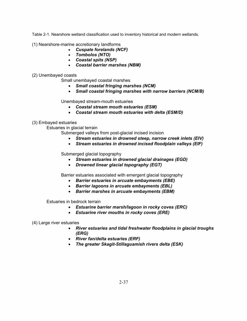
Table 2-1. Nearshore wetland classification used to inventory historical and modern wetlands.

(1) Nearshore-marine accretionary landforms Cuspate forelands (NCF) Tombolos (NTO) Coastal spits (NSP) Coastal barrier marshes (NBM)

(2) Unembayed coasts Small unembayed coastal marshes

Small coastal fringing marshes (NCM)

Small coastal fringing marshes with narrow barriers (NCM/B)

Unembayed stream-mouth estuaries

Coastal stream mouth estuaries (ESM)

Coastal stream mouth estuaries with delta (ESM/D)

(3) Embayed estuaries Estuaries in glacial terrain

Submerged valleys from post-glacial incised incision

Stream estuaries in drowned steep, narrow creek inlets (EIV)

Stream estuaries in drowned incised floodplain valleys (EIF)

Submerged glacial topography

Stream estuaries in drowned glacial drainages (EGD)

Drowned linear glacial topography (EGT)

Barrier estuaries associated with emergent glacial topography

Barrier estuaries in arcuate embayments (EBE)

Barrier lagoons in arcuate embayments (EBL)

Barrier marshes in arcuate embayments (EBM)

Estuaries in bedrock terrain

Estuarine barrier marsh/lagoon in rocky coves (ERC)

Estuarine river mouths in rocky coves (ERE)

(4) Large river estuaries

River estuaries and tidal freshwater floodplains in glacial troughs (ERG)

River fan/delta estuaries (ERF)

The greater Skagit-Stillaguamish rivers delta (ESK)

2-37

Table 2-2. An example key for assigning wetland complexes to one of 20 types.

1. Estuary of a major river (If NO, continue to 2) 1a. Glacial trough (ERG) 1b. Steep fan delta (ERF) 1c. Part of Samish-Skagit-Stillaguamish delta system. (ESK)

2. Embayed (If NO, go to 6)

3. Glacial or bedrock terrain (If GLACIAL, continue to 4) 3a. Marsh or lagoon, small or no stream, beach in arcuate rocky cove (ERC) 3b. River in arcuate rocky cove (ERE) 3c. Otherwise, continue to 4

4. Postglacial fluvial erosion (If NO, continue to 5) 4a. Narrow V-shaped valley (EIV) 4b. Wider floodplain valley (EIF)

5. Wetland created by glacial topography (If NO, continue to 6) 5a. Linear depression 5a-i. Stream estuary in glacial drainage (EGD) 5a-ii. Drowned glacial topography (EGT) 5b. Barrier estuary in arcuate embayment 5b-i. Partial barrier (EBE) 5b-ii. Full barrier 5b-ii.1 Large central lagoon (EBL) 5b-ii.2. Primarily marsh (EBM)

6. Unembayed (If CONVEX ACCRETIONARY, continue to 7) 6a. Mouth of steep unembayed stream 6a-i. No delta (ESM) 6a-ii. Small delta (ESM/D) 6b. Coastal fringing marsh 6b-i. No barrier (NCM) 6b-ii. Barrier (NCM/B)

7. Accretionary landforms 7a. Connecting two land masses (tombolo) (NTO) 7b. Attached to land at one end (spit) (NSP) 7c. Cuspate (cuspate foreland) (NCF) 7d. Nearshore barrier marsh (NBM)

2-38

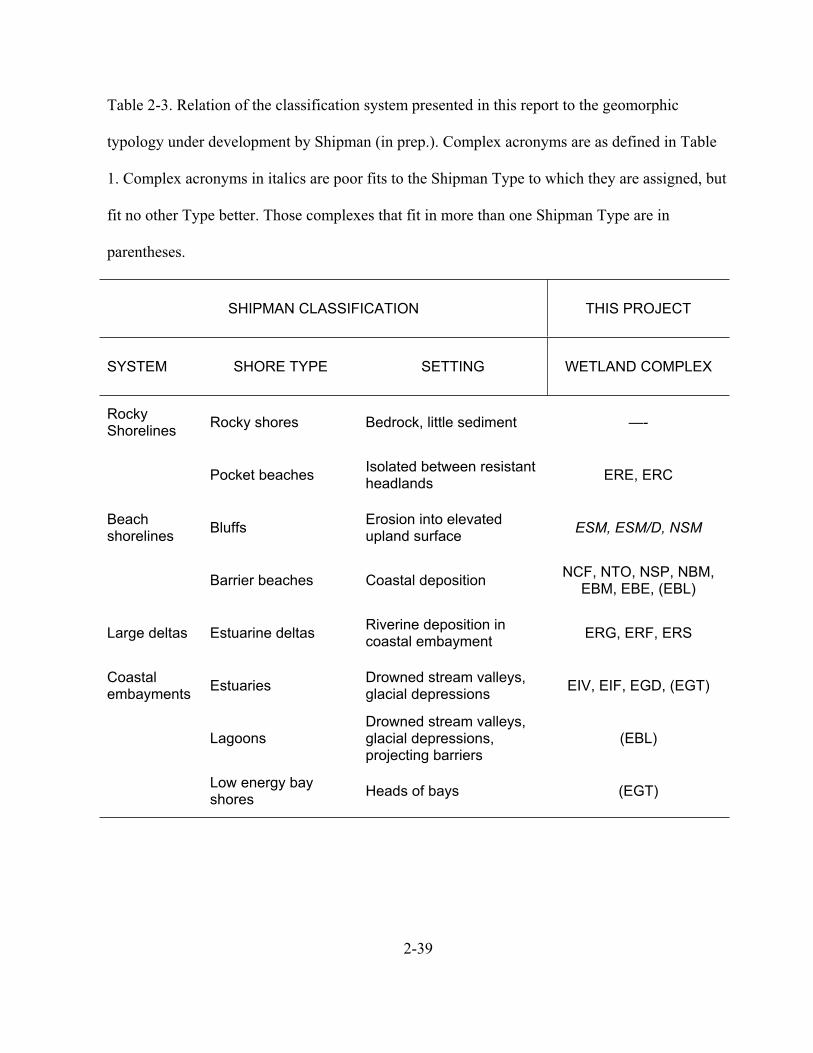
Table 2-3. Relation of the classification system presented in this report to the geomorphic

typology under development by Shipman (in prep.). Complex acronyms are as defined in Table

1. Complex acronyms in italics are poor fits to the Shipman Type to which they are assigned, but

fit no other Type better. Those complexes that fit in more than one Shipman Type are in

parentheses.

SHIPMAN CLASSIFICATION THIS PROJECT

SYSTEM SHORE TYPE SETTING WETLAND COMPLEX

Rocky Shorelines

Rocky shores Bedrock, little sediment —-

Pocket beaches Isolated between resistant headlands

ERE, ERC

Beachshorelines

BluffsErosion into elevated upland surface

ESM, ESM/D, NSM

Barrier beaches Coastal deposition NCF, NTO, NSP, NBM,

EBM, EBE, (EBL)

Large deltas Estuarine deltas Riverine deposition in coastal embayment

ERG, ERF, ERS

Coastalembayments

EstuariesDrowned stream valleys, glacial depressions

EIV, EIF, EGD, (EGT)

Lagoons Drowned stream valleys, glacial depressions, projecting barriers

(EBL)

Low energy bay shores

Heads of bays (EGT)

2-39

Figure Captions

Figure 2-1. Sub-basins and major rivers of the Puget Sound region.

Figure 2-2. Factors that create different types of tidal wetlands and some defining characteristics.

Figure 2-3. Areas of historical wetland complexes. Two complex types, river estuaries in glacial

troughs (ERG) and the Samish-Skagit-Stillaguamish deltas (ESK) are excluded from the figure

because of the great size of complexes in these types. Two values for the “EBE” type, 179 ha and

145 ha, are not shown. Numbers are sample size. Each box encloses 50% of the data. Horizontal

line within box represents median. The lines extending from the top and bottom of boxes indicate

minimum and maximum values, excepting outlier values (circles) greater than the inner quartile

plus 1.5 times the inner two quartiles.

Figure 2-4. Historical distribution of complex types. Acronyms are defined in Table 1.

2-40

2-41

Figure 2-1

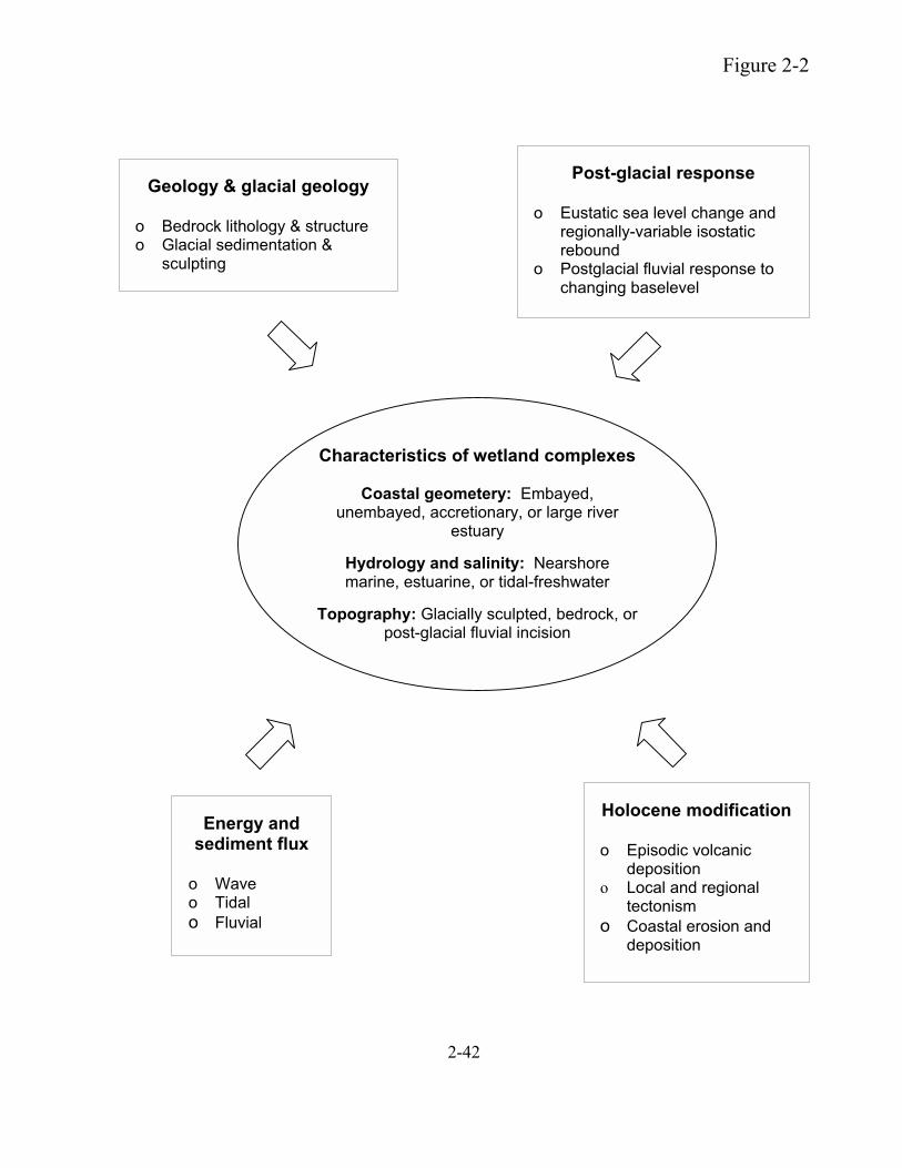
2-42

Figure 2-2

mar ter

Characteristics of wetland complexes

Coastal geometery: Embayed,unembayed, accretionary, or large river

estuary

Hydrology and salinity: Nearshoreine, estuarine, or tidal-freshwa

Topography: Glacially sculpted, bedrock, or post-glacial fluvial incision

Post-glacial response

o Eustatic sea level change and regionally-variable isostatic rebound

o Postglacial fluvial response to changing baselevel

Geology & glacial geology

o Bedrock lithology & structure o Glacial sedimentation &

sculpting

Holocene modification

o Episodic volcanic deposition

o Local and regional tectonism

o Coastal erosion and deposition

Energy and sediment flux

o Wave o Tidal

o Fluvial

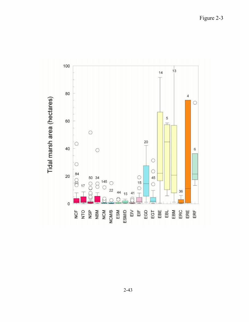
2-43

Figure 2-3

2-44

Figure 2-4

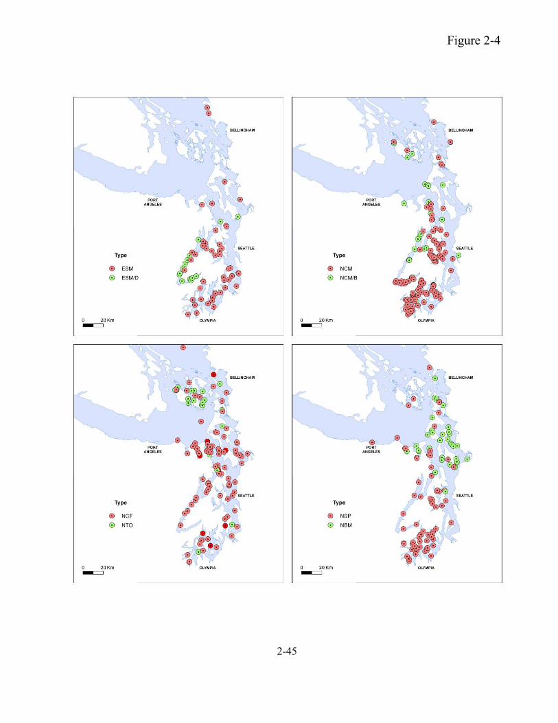
2-45

Figure 2-4

3-1

Chapter 3: Tidal wetlands in the Puget Sound region prior to Euro-

American-settlement (mid- 19th

century) compared to current conditions

Abstract

The historical amount, distribution and functions of tidal marshes in the Puget Sound region

were reconstructed for nearshore environments in the Puget Sound region representative of the

time of earliest Euro-American settlement. We identified 29,500 hectares of tidal wetland

including 12,000 hectares of estuarine emergent marsh, 6,000 hectares of estuarine scrub-shrub

wetland, and 11,500 hectares of tidal-freshwater wetlands. The estuaries of large rivers

accounted for 90% of this total. The Skagit River alone accounted for 37% of the total, and the

Snohomish River estuary an additional 22%, when combined with the nearby Samish and

Stillaguamish river estuaries; these four adjacent rivers accounted for 74% of the total. The steep,

narrow fan-delta estuaries draining the Olympic Mountains to Hood Canal and the Strait of Juan

de Fuca accounted for only 1% of the total area of tidal marsh around Puget Sound. Outside

these river valleys, wetlands associated with accretionary landforms and with barrier estuaries in

arcuate embayments associated with emergent glacial terrain, more abundant in high wave

energy environments of the northern study area, accounted for 3% and 4% of the region’s tidal

marsh, respectively. Drowned glacial drainages accounted for the largest portion of tidal marsh

in the southern Sound, which is characterized by lower energy environments and a rising post-

glacial sea level. The effects of Pleistocene glacial erosion and sedimentation, Holocene volcanic

deposition, and the ongoing effects of wave and current energy are the primary controls on the

relative sizes and spatial distribution of wetlands. An 1884 inventory of pre-settlement tide

3-2

marsh agrees with our total estimate within 1-2%. Tidal wetlands are now about 17-19% of their

historical extent, including wetlands created since the historical reference condition. Both the

number and sizes of wetlands have diminished. About half of current tidal marsh is concentrated

in the greater Skagit River delta area, proportionately nearly as much as historically. In contrast,

rivers in glacial troughs account for a smaller portion of the total than they did historically,

reflecting the substantial loss in area from the Lummi, Duwamish, and Puyallup river estuaries.

Other wetland types in aggregate have experienced a smaller relative decline. Some wetland

types have lost much more than others, notably the large barrier marshes in arcuate embayments

in the north Sound. Change was not uniform spatially; of the different sub-basins, the northern

Sound and Central Sound sub-basins have the least of their historical wetland area remaining

proportionally, and the Hood Canal, South Sound and West Strait sub-basins have proportionally

the most remaining tidal wetland.

Introduction

Statement of the problem

There is at present an incomplete understanding of the historical amount, types, distribution,

and sizes of tidal marshes that existed in Puget Sound prior to the land use transformation that

began with Euro-American settlement in the mid 19th

century. Such information would provide

insight into the structure and function of wetlands in environments for which there are few or no

analogs, and would contribute to the basis for quantifying lost biological productivity from tidal

wetland conversion in determining restoration targets for endangered species. Spatially explicit

information would also provide a template for guiding wetland restoration in parts of the

3-3

nearshore environment that have been most transformed. In addition, there has been no

comprehensive accounting of the amounts and causes of change to the region’s tidal wetlands.

To characterize historical wetlands and to compare their abundance and distribution to the

present, we reconstructed historical environments using primarily archival sources with a

Geographic Information Systems (GIS), and for comparison created a comparable GIS map of

current conditions.

Approach to reconstructing historical conditions

To make an inventory of historical tidal wetlands, we reconstructed the Puget Sound region’s

native nearshore environment using a GIS and a number of methods and sources, primarily

historical; methods are described in Chapter 1 of this report. Briefly, to achieve spatially

comprehensive coverage, we began by creating a geospatial digital database from topographic

sheets (T-sheets) surveyed by the US Coast & Geodetic Survey (USC&GS) in the period

between 1850 and 1900. We supplemented these maps with a number of other sources because

there had already been a great deal of land conversion by the time of the USC&GS work, the T-

sheet mapping did not generally extend inland in river valleys to include the entire estuary, and

because it is desirable to augment the T-sheets and to cross-check them. Other sources and

methods we used included the federal land surveys made in the 1850-1880 period, soil surveys,

1930s aerial photographs, other early maps, and various text sources. We were also able to cross-

reference our estimates of pre-settlement tidal marsh with an early inventory of pre-settlement

condition of tidal marshes published in 1885 (Nesbit 1885). To provide a basis for comparing our

reconstruction of historical conditions to the current landscape, we also created a GIS

3-4

geodatabase of current conditions, primarily digitized from recent (1998-2000) aerial

photographs in a manner designed to be comparable to the historical materials in detail.

Here we present a regional overview of the historical amounts, types and distributions of

tidal wetlands and how these differ at present. The accompanying GIS data upon which this

gross analysis is based can be used both for site-specific historical reconstruction and, along with

descriptions made for intermediate time periods, to describe change at a smaller scale (see for

example Collins, 2005).

Previous inventories of historical tidal wetlands in Puget Sound

Newspaper publisher Eldridge Morse, an early resident of the Snohomish River valley, made

the first published inventory of tidal marsh (inclusive of saltmarsh and tidal freshwater marsh;

see p. 6, Nesbit 1885) in the greater Puget Sound area. Morse provided an inventory of Puget

Sound tidal marsh for a federal survey of tidal marshes (Nesbit 1885). Morse’s inventory

included extensive descriptions, especially of the larger river estuaries in eastern Puget Sound,

and a quantitative summary. Probably completed in 1884, Morse’s assessment was also an early

change analysis; by his estimates, 38% of the Puget Sound region’s tidal marsh had already been

diked and reclaimed for agriculture. Morse’s estimates are discussed in detail later in this

chapter.

More recently, researchers have used the USC&GS T-sheets to inventory the historical extent

of tidal marshes in different regions of the United States (e.g., see Atwater et al. 1979 for

summary of investigations in the San Francisco Bay area). In the Puget Sound region, a federal

study published in 1980 (Bortleson et al. 1980) used primarily T-sheets to estimate retrospective

3-5

change to tidal marshes (“subaerial” and “intertidal” wetlands) at eleven river deltas in the Puget

Sound region. The 1980 study quantified undiked marsh at the time of the T-sheets surveys,

made in the 1855-1899 period, and makes partial estimates of diked tide marshes not shown on

the T-sheet surveys. Thom and Hallum (1990) summarized and synthesized the data from the

Morse and Bortleson et al. studies. In an early phase of this study (Collins et al. 2003) we

reported on reconstructions of the historical environments of several river estuaries in northern

Puget Sound; the reconstruction showed that a considerable amount of land had been converted

to agriculture prior to the T-sheets, especially estuarine scrub-shrub and riverine-tidal

environments.

Approach to structuring data

Chapter 2 presents our approach to organizing data from our reconstruction of tidal wetlands.

At the largest scale, we created 10 sub-basins, based in part on the oceanographic basins of

Burns (1990), as described in Chapter 2, and shown in Figure 2-1. At the next smallest scale, we

defined 20 typical wetland complexes, based on the geologic terrain, the topography created by

glaciation, post-glacial changes in land and sea level and the erosional responses, the coastal

geometry (accretionary, unembayed, or embayed), the dominance of fluvial versus wind and

current energy, and whether the environment was marine, estuarine, or tidal freshwater. The

resulting classification is summarized in Table 2-1. The 20 distinct wetland types are grouped

into four major settings: (1) coastal landforms (cuspate forelands, coastal spits, tombolos, and

small coastal fringing marshes); (2) non-embayed stream mouth estuaries; (3) embayed estuaries,

marshes and lagoons (exclusive of the major rivers draining the Cascades and Olympics); and (4)

major river estuaries, which include in some cases extensive tidal freshwater floodplains.

3-6

Embayed estuaries, marshes and lagoons make up the largest grouping. Because it includes a

variety of landform settings, it is further subdivided into three sub-groupings reflecting

differences in geologic and base level histories (Table 2-1).

Within the larger complexes, we created identification codes for individual features,

identified with unique numbers within townships. We recorded detailed narrative descriptions of

wetland complexes and features, including the historical data available to us, and the

assumptions we made in using the data. These descriptions are coded for use in conjunction with

the GIS coverages.

Historical tidal wetlands in the Puget Sound region

Amount, type, and distribution

We mapped a total of 29,500 hectares of tidal marsh from 621 wetland complexes (Table 3-1

and Figure 3-1). This total leaves out a number of locations where wetlands are likely or certain

to have existed but we lacked enough evidence at this time to map them; while this makes 621 a

minimum number, because most of the unmapped wetlands are small, it does not significantly

affect the aggregate wetland area. We included the area of blind tidal channels in our marsh area

totals, and excluded other types of channels. Of the total, 42% was estuarine emergent marsh,

20% was estuarine scrub-shrub marsh, and 38% was tidal freshwater marsh (Table 3-1). A large

amount of the total, 18,300 hectares, or 62%, was concentrated in the Whidbey Basin (Figure 3-

2); the Whidbey Basin excludes the portion of the Skagit River that drained to Padilla Bay, and

excludes the Samish River delta, both of which are counted in the San Juan Island/North Coast

3-7

sub-basin totals, but are both physiographically part of the greater Skagit River delta. If the

Padilla Bay and Samish River tidal marsh were included in the Whidbey Basin total, it would

total 22,400 hectares or 76% of the region’s total.

Tidal wetlands were also heavily concentrated in the estuaries of the basin’s major rivers.

The major rivers draining the Cascade Range and Olympic Mountains accounted for 90% of the

tidal wetland (Table 3-2). Over half of the region’s tidal wetland area (53%) was in the wetland

complex “ESK” that includes the deltas of the Stillaguamish, Skagit, and Samish rivers. [The

text and accompanying figures uses area, in hectares, and frequency, the number of wetland

complexes, as metrics.] As described in Chapter 2, these deltas were grouped together because

the Skagit and Samish are both on the same delta created by massive mid-Holocene lahar

deposition, and the Stillaguamish delta is continuous with the Skagit delta, and was also likely

influenced by volcanic sedimentation. Seven major rivers within broad, low-gradient troughs

created by sub-glacial fluvial erosion—the Lummi, Nooksack, Snohomish, Duwamish, Puyallup,

Nisqually, and Skokomish—accounted for another 37% of the regional total (Table 3-2). The

remaining major Olympic Peninsula rivers—the steep, narrow fan-deltas of the Hamma Hamma,

Duckabush, Dosewallips, Quilcene, Dungeness, and Elwha rivers—accounted for only 1% of the

regional total.

Primarily because of the dominant quantitative influence of the large river estuaries, tidal

wetland area was unequally distributed throughout the study area (Figure 3-3). The four sub-

basins lacking major rivers—the Western Inlets, Admiralty Inlet, Eastern Strait and Western

Strait sub-basins—had a small fraction of the marsh in the other sub-basins, making it useful to

consider the distribution of major rivers estuaries separately from the other complexes. Figure 3-

3-8

3, which shows the relative size of estuarine wetlands in the major river estuaries, reiterates the

dominant importance of the Stillaguamish-Skagit-Samish deltas system, followed by the rivers in

subglacial troughs, which in turn dwarf the east and north Olympic Mountains river estuaries. It

also shows that, more generally, the area of tidal marsh associated with rivers in the north half of

the study is much greater than the amount in the remainder of the study area. Among the river

estuaries in glacial troughs in the southern part of the study area, the Puyallup and Nisqually

estuaries had much more tidal marsh than the Duwamish. The figure also shows that the northern

rivers were also unique in having more scrub-shrub wetland, and more riverine-tidal freshwater

wetland than elsewhere in the study area. Thus the northern Sound river estuaries were both

larger and more diverse than elsewhere.

The other 17 tidal wetland types described in Chapter 2 accounted for the remaining 10% of

regional tidal marsh area. Of this amount (which when added to the Olympic Peninsula fan

rivers, account for 11% of the total; see Table 3-2), the large barrier marshes and lagoons in

arcuate embayments in the northern Sound accounted for the largest amount, about two-fifths

(Table 3-3). Tidal wetlands associated with accretionary landforms—spits, cuspate forelands,

tombolos, and non-estuarine accretionary barrier wetlands—accounted for the next largest

amount, nearly one quarter of the total, or 23%. Estuaries in drowned glacial topography,

common in the southern half of the study area, accounted for 17% of area, the next largest

amount; about two thirds of this amount was in the drowned glacial drainages generally located

at the ends of the region’s major inlets. The fan-deltas of the Olympic Peninsula rivers listed

above accounted for another 6% of the total. The remaining five types of tidal wetlands

altogether accounted for the remaining 17%.

3-9

While quantitatively less important, the wetland types that were generally small were much

more numerous than the wetland types that were generally larger; Table 3-3 shows the number of

wetland complexes by type and sub-basin. The smallest features—the unembayed coastal

marshes and stream mouth wetlands—accounted for 34% of the total number of individual

wetland complexes. The same was true of wetlands in incised stream valleys, which accounted

for 12% of the total. On the other hand, the largest wetland complexes not associated with major

rivers, the barrier wetlands in arcuate depressions in emergent glacial terrain, accounted for only

7% of the total number of complexes; the large complexes in the major river valleys of eastern

Puget Sound were the least frequent, accounting for only 2%.

There are north-to-south and other regional differences among the 10 sub-basins in the

distribution of non-large-river tidal wetland complexes (Figure 3-4 and Figure 3-5). Most of the

tidal wetlands in the northern sub-basins are within the generally large barrier estuaries in arcuate

embayments in emergent glacial terrain or associated with accretionary landforms, particularly

cuspate forelands, which also tended to be large in the north. The North Coast/San Juan Island

area is anomalous in the north in having tidal wetlands distributed within a broader range of

environments, including the rocky coves unique to this area and the Western Strait sub-region.

This greater diversity in environments reflects the dominance of bedrock terrain intermixed with

the influence of glacial sculpting, especially in the transitional margins of the sub-basin, and the

diversity of energy environments. In contrast with the other northern sub-basins, the small

amount of tide marsh in the Western Strait was within the rocky-cove estuaries of small coastal

and foothill streams.

3-10

In the southern half of the Puget Sound region, tidal wetlands are primarily within lower

energy environments: drowned glacial drainages or other drowned glacial topography, within

drowned incised valleys, as small, unembayed coastal marshes, and small stream-mouth

estuaries. The South Sound and Western Inlets sub-regions are the most dominated by lower-

energy environments, and the environments of wetlands in the Central Sound and Hood Canal

sub-regions are a mix of higher and lower energy levels. The generally smaller wetland

complexes in the southern part of the region were more numerous compared to the generally

larger features in the north (Figure 3-5). As indicated previously, in general the smaller features,

which were more common in the south, were more numerous than the larger features. Figure 3-6

shows the relative areas of individual tidal wetland complexes historically in the study area,

including major rivers (Figure 3-6A) and exclusive of them (Figure 3-6B); the area of the circle

symbols in the figures are proportional to the wetland area.

Comparison to an 1884 inventory of tidal marsh in Puget Sound

Eldridge Morse’s 1884 retrospective estimate of tidal marshes, described previously in this

report, provides a check on our estimates that is unique in having been compiled within the first

decades of the great land transformation associated with Euro-American settlement. It is also

independent of our reconstruction; we used Morse’s descriptions only locally with a few smaller

wetlands and to supplement our map data. In addition to containing a great deal of descriptive

information, Morse reported the size of most of the larger or more conspicuous tidal wetlands.

His assessment is particularly detailed in the Snohomish, Stillaguamish and Skagit river deltas,

reflecting their quantitative importance, and probably as well his residence in the village of

Snohomish, which would have provided him a greater opportunity to examine his local rivers.

3-11

At the end of his systematic assessment, Morse provides a summary table, organized by

county. The entries in his table total 28,800 hectares, although in the text he gives numbers that

total 29,100 hectares. Depending on which of these is taken as the total, our estimate of 29,500

hectares agrees within either 1% or 2% of Morse’s total (Table 3-4). Our estimates agree most

closely with Morse’s estimates for Skagit County, which is where we have made our most

detailed reconstruction, and where Morse made one of his most detailed examinations. On the

other hand, our estimates agree the least with his in the Snohomish River estuary; it appears that

the difference in the two estimates is because we interpreted more of the Snohomish’s freshwater

wetland as tidally influenced than Morse did, apparently the “Marshland” district in particular, so

that the discrepancy between our estimates for the Snohomish estuary reflect differences in

hydrologic interpretation rather than in map area. In a few counties where our estimates are less

than Morse’s, the difference can be accounted by our having conservatively mapped a few

wetlands that had been heavily urbanized in the 19th

century, for example we mapped Salmon

Bay’s tidal wetlands conservatively, likely accounting for the difference in the two estimates for

King County. After the Snohomish, the greatest discrepancy is in the east-Sound counties that he

grouped together—Mason, Kitsap, Jefferson and Clallam counties, where Morse’s estimate is

greater than ours—which may reflect less detailed knowledge on Morse’s part because of their

distance and smaller quantitative importance. In any case, the two estimates are remarkably

consistent overall.

Comparison to other estimates for Puget Sound

Eldridge Morse’s study has received considerable less attention than the map study made a

quarter-century ago by Bortleson et al. (1980). Made by hand-registering T-sheets and early

3-12

USGS topographic maps to modern topographic maps, and measuring the wetland area on the

modern maps, the 1980 study focused on 11 river deltas. In comparing our estimates to those in

the 1980 study, we have dropped the Dungeness River from the list because it is a small estuary;

the 1980 report appears to have erroneously indicated the size of the Dungeness River tidal

marsh as 10 times greater than supported by their map data and our reconstruction.

Table 3-5 compares our estimates with those published by Bortleson et al. (1980). The 1980

study differentiated “intertidal” and “subaerial” wetlands without definition, complicating

comparison. Our estuarine wetland estimate is about two and half times greater than in the 1980

study, 152 km2 compared to 62 km

2. The discrepancy is in large part because the earlier study

didn’t estimate intertidal wetlands in the Samish, Skagit, or Stillaguamish river deltas, which had

been heavily diked by the time of the USC&GS surveys in the mid 1880s, and because they

excluded the expansive marshes to the north of the Skagit River’s North Fork. On the other hand,

the earlier study overestimates the historical estuarine marsh in some estuaries. An overestimate

of the Duwamish River’s intertidal marsh is apparently from misinterpreting the T-sheet

symbology as saltmarsh on what was a fir-covered terrace located several meters above the

floodplain and probably created by uplift during the Seattle Fault earthquake ca. 1,100 yr B.P.

and subsequent fluvial downcutting. Elsewhere they interpret as intertidal marshes areas that we

have mapped as freshwater marsh.

Their “subaerial” category includes tidal-freshwater as well as some of what we map as

palustrine wetlands. To facilitate a comparison, we include in Table 3-5 palustrine wetlands that

we mapped on the floodplain within the up-valley extent of tidal river influence, which

encompasses the broader “nearshore wetland” category defined earlier in this report. We

3-13

included in this category all floodplain wetlands within the valley bottom where the main river is

tidally influenced, so as to include wetlands that are palustrine rather than riverine-tidal in that

they are not regularly inundated on a tidal cycle, but would be more frequently flooded during

high water because of the augmenting effect of tidal backwater on floods. Without resolving

ambiguities that arise from comparing the two estimates, our estuarine wetland estimate is two

and a half times greater than the 1980 estimate, and our “nearshore wetland” total (332 km2) is

half again as much as their higher estimate (202.6 km2) and twice their low estimate (152 km

2).

The geology of tidal wetlands

Several geologic influences together substantially explain the distribution, amount, and type

of tidal wetlands. The quantitatively most important, if spatially most concentrated, influence is

that of volcanic deposition. As described in the previous chapter, the greater Skagit River delta

was largely created during a mid-Holocene eruptive period of Glacier Peak, and the

Stillaguamish River delta at least in part so. Similar mid- and late-Holocene lahar deposition

from Mt. Rainier prograded the Duwamish and Puyallup embayments and created low-gradient

estuaries; Mt. Baker lahars may have contributed to the Nooksack and Lummi deltas. Volcanic

eruptions created the topography on which more than half of the region’s historical tidal marsh

developed.

In contrast to the spatially concentrated influence of volcanic deposition, the glacial legacy is

the most pervasive influence, and at numerous scales. Sub-glacial fluvial erosion created the

wide, low-gradient troughs in which the large river estuaries are located. Smaller-scale erosional

features provide the template for wetlands, especially in the southern study area, where they have

3-14

been drowned during the post-glacial rise in sea level. Coastal streams that have incised through

the glacial fill to create valleys, later partially flooded, create additional estuarine environments.

In the northern Puget Lowland, the combination of post-glacial land emergence, linear glacial

topography, and coastal processes during sea level rise created the arcuate embayments where

the largest non-riverine wetlands are located.

Wave and current energy, in interaction with an inexhaustible supply of readily erodible sand

and gravel from shore bluffs of glacial deposits, is the third major influence. The resulting

accretionary and barrier landforms provide the physical template for more than half of the tidal

wetlands outside of the river valleys overall, and a considerably larger proportion in the northern

part of the region. While additional factors are locally important, including recent tectonism

associated with the system of faults that dissects the Puget Basin, and the effects of regional

plate-tectonic strain, these three forces—volcanic deposition, the glacial legacy, and wave

energy—are the most dominant. They are most coincident in the Whidbey Basin, which accounts

for that basin’s great concentration of tidal wetland.

Biogeographic and ecological implications

Regional gradients characterized the amount, distribution, and type of tidal marsh. Tidal

marsh habitats were characterized by relative dispersal and concentration over at least two scales.

On the scale of the Puget Sound region, tide marsh was concentrated within the Whidbey Basin.

In a broad north-to-south gradient within the basin, habitats were either concentrated in more

dispersed, larger complexes, or less dispersed in more frequent, smaller complexes in lower-

energy environments typical especially of the Southern Sound and Western Inlets and much of

3-15

Hood Canal. There were also differences within the region in the distance with which tidal

wetlands were dispersed relative to the large river mouths, and consequently access to extensive

freshwater habitats.

The diversity of tidal marsh salinity environments was spatially patchy; the abundance of

estuarine scrub-shrub wetlands and tidal freshwater wetlands conspicuously clusters in the north

Sound rivers from the Snohomish to the Lummi-Nooksack river estuaries. Among the large

rivers, the amount of tidal marsh was not proportional to the size of the river system (and the

extent of its freshwater habitats), being determined instead by other, largely independent factors.

Comparison to the current condition

To compare to the current condition, we mapped wetlands at 460 of the historical complexes,

using recent aerial photographs and the National Wetlands Inventory (NWI; see Chapter 1).

Figure 3-7A shows the historical wetland complexes where we did not map tidal wetland from

the recent photographs and NWI, and Figure 3-7B shows sites which we had identified as likely

to have had wetlands historically, but where we lacked evidence to map them, but where

wetlands were found in the current data.

We mapped an aggregate total of 5,650 hectares (Table 3-6). We have not at this time

separated the amounts of tide marsh newly developed since the historical period from marsh that

has been lost, or the causes of loss. Earlier, Boule et al. (1983) derived an estimate of 4,980

hectares of estuarine wetland by compiling published map sources [4,745 hectares of emergent

marsh, 11 hectares of scrub-shrub, and 225 hectares of forested wetland]. Because of time

constraints we have not evaluated the source of the discrepancy between the two estimates.

3-16

Aggregating losses in area with gains in area from newly accreted marshes, if our estimate is

used, tidal marsh currently is 19% of the amount mapped historically; if the earlier estimate is

used, there is 17% of the historical amount.

The size distribution of wetland complexes has shifted downward. Wetland complexes are

generally smaller now than historically, with a median size about three-fifths the historical size,

0.93 hectares compared to 0.57 hectares (Figure 3-8A). The aggregate amount of tidal marsh in

the very largest complexes declined disproportionately more, as did the amount of tidal marsh in

the very smallest complexes (Figure 3-8B).

The deltas of the Skagit, Stillaguamish and Samish rivers quantitatively dominates the

regional tide marsh nearly as much as it did historically, now accounting for 51% of the total,

compared to 52% historically (Tables 3-7 and Figure 3-9). However, the estuaries of rivers in

large glacial troughs account for a smaller portion of the total now than historically, totaling 23%

of the regional total now, compared to 37% historically. The steep-fan river estuaries of the

Olympic Peninsula constitute a relatively greater proportion of the total than they did

historically, totaling 5% now compared to 1% historically. Figure 3-10 shows graphically the

distribution of tidal wetland area among the estuaries of major rivers indicated by our current

conditions mapping; to facilitate visual comparison with Figure 3-3, both figures have the same

symbol scale. The disproportionate loss of tidal wetland from the estuaries in large glacial

troughs is accounted for by the dramatic declines in the Lummi and Puyallup rivers. While the

loss of tidal marsh in the Duwamish estuary is nearly total, the absolute amount was relatively

small because the historical amount was relatively small compared to other estuaries in its

category.

3-17

Tidal marsh located elsewhere than the estuaries of large rivers accounts for twice the

proportion for which it accounted historically, 21% now compared to 10% historically (Tables 3-

6 and 3-2). This relative gain in importance reflects relatively small losses in some sub-basins

relative to others (Figure 3-11 compared to Figure 3-4). The South Sound, Hood Canal, Western

Strait sub-basins have lost the least wetland (from complexes exclusive of the major rivers). The

Central Sound, Fraser Lowland, and Whidbey Basin have lost the most proportionately. In the

South Sound and Hood Canal the wetlands in drowned glacial drainages account for the largest

amount of the totals (Figure 3-11), and relatively more than historically (Figure 3-4). In the

Fraser Lowland, Admiralty Inlet and Whidbey Basins the barrier wetlands in arcuate

embayments have become proportionately less significant, and wetlands in accretionary

landforms have become proportionately more important; wetlands in accretionary landforms

have also become proportionately more significant in the East Strait and San Juan Islands/North

Coast sub-basins. Figure 3-12A shows the spatial distribution and size of individual wetlands;

compared to Figure 3-6A, it shows the notable losses in wetland area in the Central Sound and

the general diminishment in the number and sizes of the larger complexes that existed in the

north Sound, and the relatively small change in the number and size of wetland in the South

Sound and Hood Canal.

Including all wetland complexes, the Whidbey Basin (which includes the Snohomish,

Skagit, and Stillaguamish rivers) has had the largest absolute decline, followed by the San Juan

Islands/North Coast (which includes the Padilla Bay part of the greater Skagit River delta, and

the Samish River), the Fraser Lowland (which includes the Lummi and Nooksack rivers), and the

Central Sound (which includes the Duwamish and Puyallup rivers; Figure 3-12A).

3-18

Proportionately, the Central Sound, San Juan Islands/North Coast, Fraser Lowland, and Whidbey

Basin all have less tidal marsh remaining than the regional average of 17-19% (Figure 3-13B).

The Central Sound also shows the greatest percentage decline in the number of complexes

remaining (Figure 3-13C), while the South Sound lost the greatest number of complexes (Figure

3-13D), primarily the smaller fringing coastal marshes, which is also the type of wetland having

lost the largest number of complexes (Figure 3-14B); Figure 3-14B also shows that overall,

wetlands in unembayed stream mouth estuaries and cuspate forelands have also been

substantially diminished in number.

In summary, tidal wetlands now amount to about 17-19% of their historical extent, including

wetlands newly created since the historical reference condition. There have been declines in both

the number and size of wetlands. About half of current tidal marsh is concentrated in the greater

Skagit River delta area, nearly as much as historically. In contrast, rivers in glacial troughs

account for a smaller portion of the total than they did historically, reflecting in large part the

substantial loss in area from the Lummi, Duwamish, and Puyallup river estuaries. Other wetland

types in aggregate have experienced less of a relative decline. Some of these wetland types have

lost much more than others, notably the large barrier marshes in arcuate embayments in the north

Sound, as have some sub-basins; the northern Sound and Central Sound sub-basins have lost the

most area proportionally, and the Hood Canal, South Sound and West Strait sub-basins have

proportionally the most remaining tide marsh.

3-19

References Cited

Atwater, B. F., S. G. Conard, J. N. Dowden, C. W. Hedel, R. L. MacDonald, and W. Savage.

1979. History, landforms, and vegetation of the estuary’s tidal marshes. In. T. J. Conomos

(ed.), San Francisco Bay: The urbanized estuary. Pacific Division, American Association for

the Advancement of Science. San Francisco, CA, p. 347-386.

Bortleson, G. C., M. J. Chrzastowski, and A. K. Helgerson. 1980. Historical changes of shoreline

and wetland at eleven major deltas in the Puget Sound region, Washington, U.S. Geological

Survey Hydrological Investigations Atlas HA-617.

Boule, M. E., N. Olmsted and T. Miller. 1983. Inventory of wetland resources and evaluation of

wetland management in western Washington. Unpublished report to Washington State

Department of Ecology, Olympia, WA, 102 p.

Burns, R. E. 1990. The shape and form of Puget Sound. Puget Sound Books, A Washington

Seagrant Publication, University of Washington Press, Seattle, WA. 100 p.

Collins, B. D. 2005. Historical geomorphology and ecology of the Dungeness River delta and

nearshore environments from the Dungeness Spit to Washington Harbor. Unpublished

Report to Jamestown S’Klallam Tribe Natural Resources Dept. 1033 Old Blyn Hwy.

Sequim, WA 98382

Collins, B. D., D. R. Montgomery, and A. J. Sheikh. 2003. Reconstructing the historical riverine

landscape of the Puget Lowland. In: D. R. Montgomery, S. M. Bolton, D. B. Booth, and L.

3-20

Wall, eds. Restoration of Puget Sound Rivers, University of Washington Press, Seattle, WA.

pp. 79-128.

Nesbit, D. M. 1885. Tide marshes of the United States. U. S. Department of Agriculture

Miscellaneous Special Report No. 7.

Thom, R. M., and L. Hallum. 1990. Long-term changes in the areal extent of tidal marshes,

eelgrass meadows and kelp forests of Puget Sound. University of Washington Fisheries

Research Institute Report FRI-UW-9008.

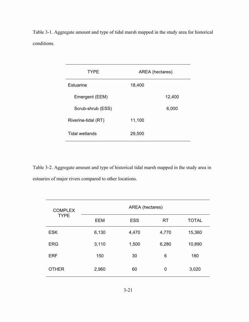
3-21

Table 3-1. Aggregate amount and type of tidal marsh mapped in the study area for historical

conditions.

TYPE AREA (hectares)

Estuarine 18,400

Emergent (EEM) 12,400

Scrub-shrub (ESS) 6,000

Riverine-tidal (RT) 11,100

Tidal wetlands 29,500

Table 3-2. Aggregate amount and type of historical tidal marsh mapped in the study area in

estuaries of major rivers compared to other locations.

AREA (hectares) COMPLEX

TYPEEEM ESS RT TOTAL

ESK 6,130 4,470 4,770 15,360

ERG 3,110 1,500 6,280 10,890

ERF 150 30 6 180

OTHER 2,960 60 0 3,020

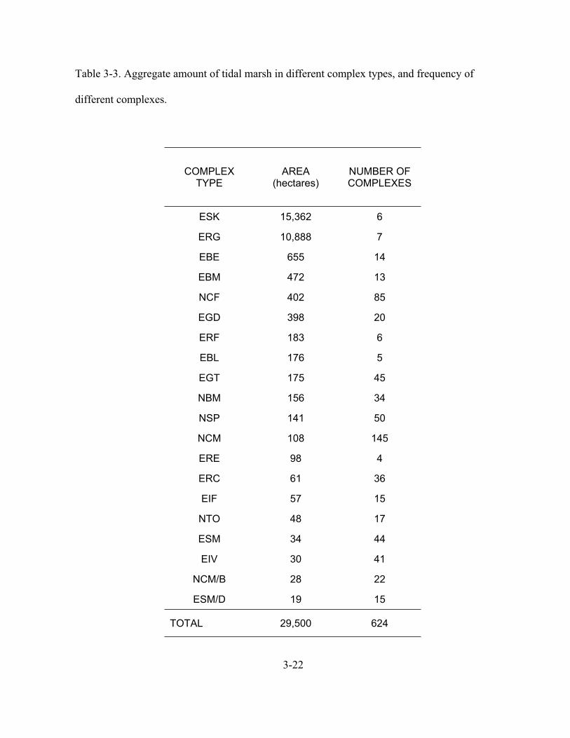
3-22

Table 3-3. Aggregate amount of tidal marsh in different complex types, and frequency of

different complexes.

COMPLEX TYPE

AREA(hectares)

NUMBER OF COMPLEXES

ESK 15,362 6

ERG 10,888 7

EBE 655 14

EBM 472 13

NCF 402 85

EGD 398 20

ERF 183 6

EBL 176 5

EGT 175 45

NBM 156 34

NSP 141 50

NCM 108 145

ERE 98 4

ERC 61 36

EIF 57 15

NTO 48 17

ESM 34 44

EIV 30 41

NCM/B 28 22

ESM/D 19 15

TOTAL 29,500 624

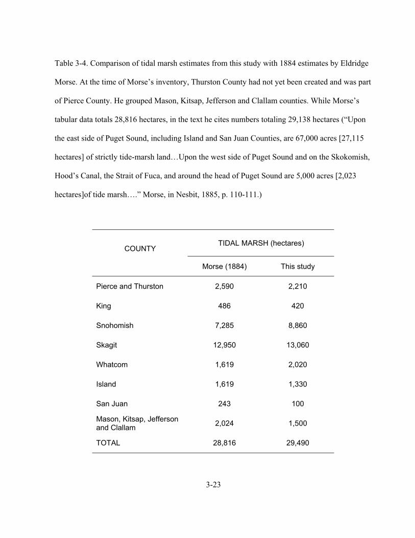
3-23

Table 3-4. Comparison of tidal marsh estimates from this study with 1884 estimates by Eldridge

Morse. At the time of Morse’s inventory, Thurston County had not yet been created and was part

of Pierce County. He grouped Mason, Kitsap, Jefferson and Clallam counties. While Morse’s

tabular data totals 28,816 hectares, in the text he cites numbers totaling 29,138 hectares (“Upon

the east side of Puget Sound, including Island and San Juan Counties, are 67,000 acres [27,115

hectares] of strictly tide-marsh land…Upon the west side of Puget Sound and on the Skokomish,

Hood’s Canal, the Strait of Fuca, and around the head of Puget Sound are 5,000 acres [2,023

hectares]of tide marsh….” Morse, in Nesbit, 1885, p. 110-111.)

TIDAL MARSH (hectares) COUNTY

Morse (1884) This study

Pierce and Thurston 2,590 2,210

King 486 420

Snohomish 7,285 8,860

Skagit 12,950 13,060

Whatcom 1,619 2,020

Island 1,619 1,330

San Juan 243 100

Mason, Kitsap, Jefferson and Clallam

2,024 1,500

TOTAL 28,816 29,490

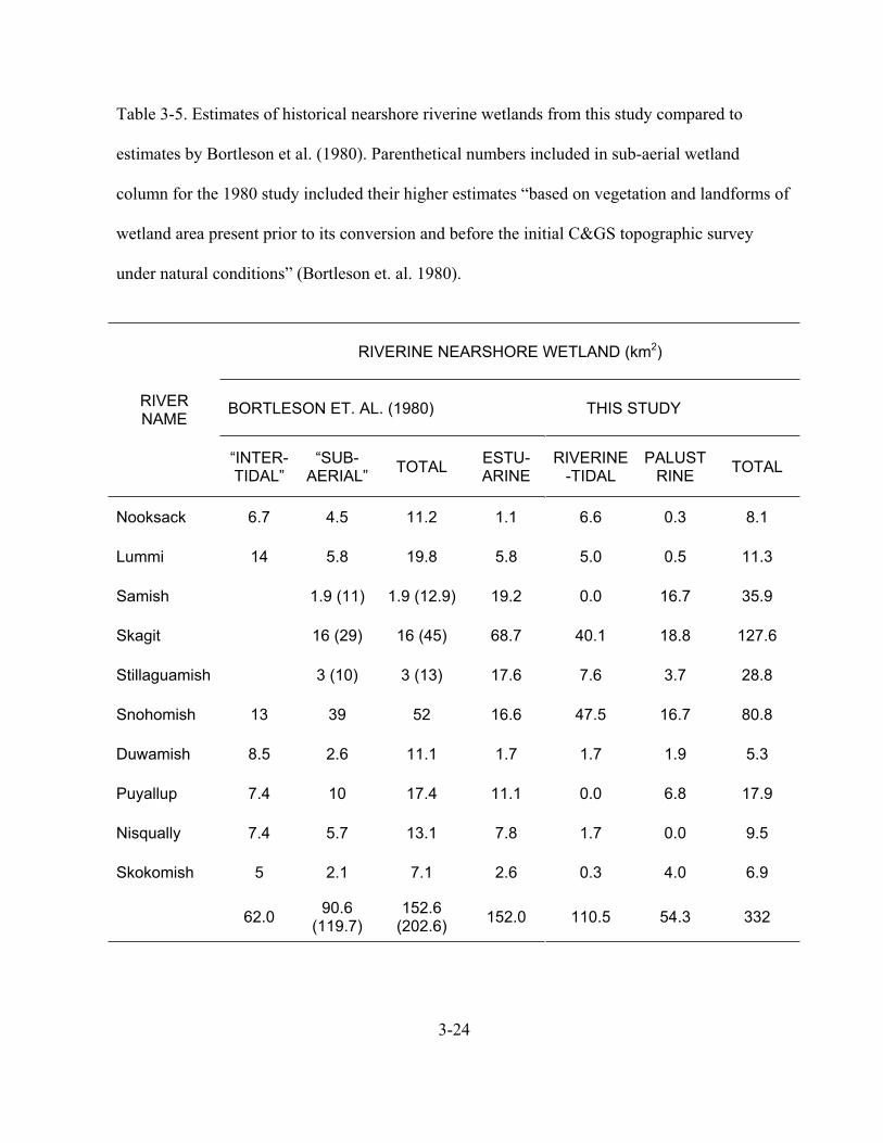
3-24

Table 3-5. Estimates of historical nearshore riverine wetlands from this study compared to

estimates by Bortleson et al. (1980). Parenthetical numbers included in sub-aerial wetland

column for the 1980 study included their higher estimates “based on vegetation and landforms of

wetland area present prior to its conversion and before the initial C&GS topographic survey

under natural conditions” (Bortleson et. al. 1980).

RIVERINE NEARSHORE WETLAND (km2)

BORTLESON ET. AL. (1980) THIS STUDY RIVERNAME

“INTER-TIDAL”

“SUB-AERIAL”

TOTALESTU-ARINE

RIVERINE-TIDAL

PALUSTRINE

TOTAL

Nooksack 6.7 4.5 11.2 1.1 6.6 0.3 8.1

Lummi 14 5.8 19.8 5.8 5.0 0.5 11.3

Samish 1.9 (11) 1.9 (12.9) 19.2 0.0 16.7 35.9

Skagit 16 (29) 16 (45) 68.7 40.1 18.8 127.6

Stillaguamish 3 (10) 3 (13) 17.6 7.6 3.7 28.8

Snohomish 13 39 52 16.6 47.5 16.7 80.8

Duwamish 8.5 2.6 11.1 1.7 1.7 1.9 5.3

Puyallup 7.4 10 17.4 11.1 0.0 6.8 17.9

Nisqually 7.4 5.7 13.1 7.8 1.7 0.0 9.5

Skokomish 5 2.1 7.1 2.6 0.3 4.0 6.9

62.0 90.6

(119.7)152.6

(202.6)152.0 110.5 54.3 332

3-25

Table 3-6. Aggregate amount and type of tidal marsh mapped in the study area for current

conditions.

TYPE AREA (hectares)

Estuarine 4,740 (84%)

Emergent 4,600 (81%)

Scrub-shrub 140 (3%)

Riverine-tidal 910 (16%)

Tidal wetlands 5,650 (100%)

Table 3-7. Aggregate amount and type of tidal marsh mapped in the study area for current

conditions in estuaries of major rivers compared to other locations.

AREA (hectares) COMPLEX

TYPEEEM ESS RT TOTAL

ESK 2,479 56 349 2,884

ERG 838 12 450 1,300

ERF 233 6 37 276

OTHER 1,052 66 76 1,195

3-26

Figure Captions

Figure 3-1. Locations of historical wetland complexes. The number of complexes is a minimum

number because it excludes locations where wetlands existed or likely existed but for which we

lacked sufficient map information. For most large river estuaries, one dot represents the estuary;

the larger and more complicated Skagit delta is represented by three complexes (the part draining

the Skagit River downstream of its forks into Skagit Bay, draining Sullivan Slough and the south

half of the Swinomish Slough to Skagit Bay, and the part draining the north half of the

Swinomish Slough and the Skagit delta north of the North Fork and into Padilla Bay), the

Stillaguamish into two (separating the wetlands on Island County from Snohomish County), and

the Dungeness with two (separating the main river mouth and the Meadowbrook Creek

distributary).

Figure 3-2. Relative area of historical tidal wetlands in different generalized complex types

compared between 10 sub-basins. The generalized types are groupings from Table 2-1. Wetland

area is proportional to the area of the pie symbol in this and subsequent figures.

Figure 3-3. Relative area, historically, of estuarine emergent, estuarine scrub-shrub, and riverine-

tidal wetlands compared between estuaries of major rivers draining the Cascade Range and

Olympic Mountains. EEM: estuarine emergent wetland; ESS: estuarine scrub-shrub wetland;

RT: riverine-tidal wetland.

Figure 3-4. Historical tidal wetland area, grouped by wetland type and aggregated in sub-basins.

Excludes estuaries of the following large rivers: complex types ESK (Skagit, Samish and

Stillaguamish rivers); ERG (rivers in glacial troughs, including the Lummi, Nooksack,

3-27

Snohomish, Duwamish, Puyallup, Nisqually, and Skokomish rivers); and ERF (steep fan/deltas

draining the eastern and northern Olympics, including the Hamma Hamma, Duckabush,

Dosewallips, Quilcene, Dungeness, and Elwha rivers). The wetland type codes are summarized

in Table 2-2 and explained in Chapter 2. Note the 10X scale change compared to the preceding

Figure 3-3.

Figure 3-5. Historical frequency of different types of tidal wetland complexes, grouped within 10

sub-basins; excludes the major river deltas listed in the caption for Figure 3-4.

Figure 3-6. (A) Historical area of individual wetland complexes. As in the other pie diagrams,

wetland area is proportional to the symbol area. (B) Panel A, but without the major river

complexes ESK and ERG, and a scale 2X that in panel (A). Excluded are types ESK (Skagit,

Samish and Stillaguamish rivers) and ERG (rivers in glacial troughs, including the Lummi,

Nooksack, Snohomish, Duwamish, Puyallup, Nisqually, and Skokomish rivers). The ERF rivers

(Hamma Hamma, Duckabush, Dosewallips, Quilcene, Dungeness, and Elwha rivers) are

included.

Figure 3-7. (A) The location of tidal wetland complexes where we identified wetlands from

recent aerial photographs and NWI data; also shown are the locations where wetlands were

mapped historically but were not evident in current data. (B) Wetland complexes mapped from

current data, but where insufficient data existed to map them historically.

Figure 3-8. Statistical distribution of the areas of individual wetland complexes currently and

historically. (A) Each box encloses 50% of the data. Horizontal line within box represents

median. The lines extending from the top and bottom of boxes indicate minimum and maximum

3-28

values, excepting outlier values (circles) greater than the inner quartile plus 1.5 times the inner

two quartiles; these outliers are not shown. (B) Cumulative size frequency of tidal marsh

complexes historically and currently.

Figure 3-9. Relative area of current tidal wetlands in different generalized complex types

compared between 10 sub-basins. The generalized types are groupings from Table 2-1. Scale is

the same as in Figure 3-2, the parallel figure for historical conditions.

Figure 3-10. Relative area, currently, of estuarine emergent, estuarine scrub-shrub, and riverine-

tidal wetlands compared between estuaries of major rivers draining the Cascade Range and

Olympic Mountains. Symbols have the same scale as those used in Figure 3-3, the parallel figure

for historical conditions.

Figure 3-11. Current tidal wetland area, grouped by wetland type and aggregated in sub-basins.

Excludes estuaries in large rivers (ESK, ERG, and ERF): complex types ESK (Skagit, Samish

and Stillaguamish rivers); ERG (rivers in glacial troughs, including the Lummi, Nooksack,

Snohomish, Duwamish, Puyallup, Nisqually, and Skokomish rivers); and ERF (steep fan/deltas

draining the eastern and northern Olympics, including the Hamma Hamma, Duckabush,

Dosewallips, Quilcene, Dungeness, and Elwha rivers). Note the factor of 2X scale change

compared to the preceding Figure 3-9. The scale of Figure 3-11 is the same as that in Figure 3-4,

the parallel figure for historical conditions.

Figure 3-12. (A) Current area of individual wetland complexes. As in the other pie diagrams,

wetland area is proportional to the symbol area. (B) Panel A, but without the major river

complexes ESK or ERG (but including complex ERF, the steep fan/delta estuaries), and a scale

2X that in panel (A).

Figure 3-13. Change in tidal wetlands from historical to current, grouped by sub-basin. (A) area

change, in hectares; (B) percent change in wetland area; (C) change in number of tidal wetland

complexes; (D) percent change in number of tidal wetland complexes.

Figure 3-14. Change in tidal wetlands from historical to current, grouped by complex type. (A)

change in area, in hectares; (B) change in number of tidal wetland complexes.

3-29

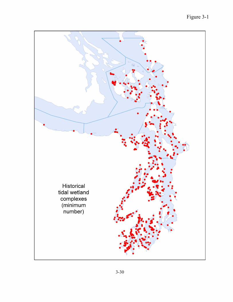
3-30

Figure 3-1

3-31

Figure 3-2

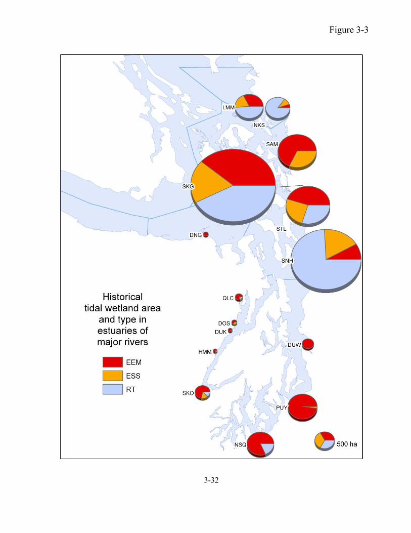
3-32

Figure 3-3

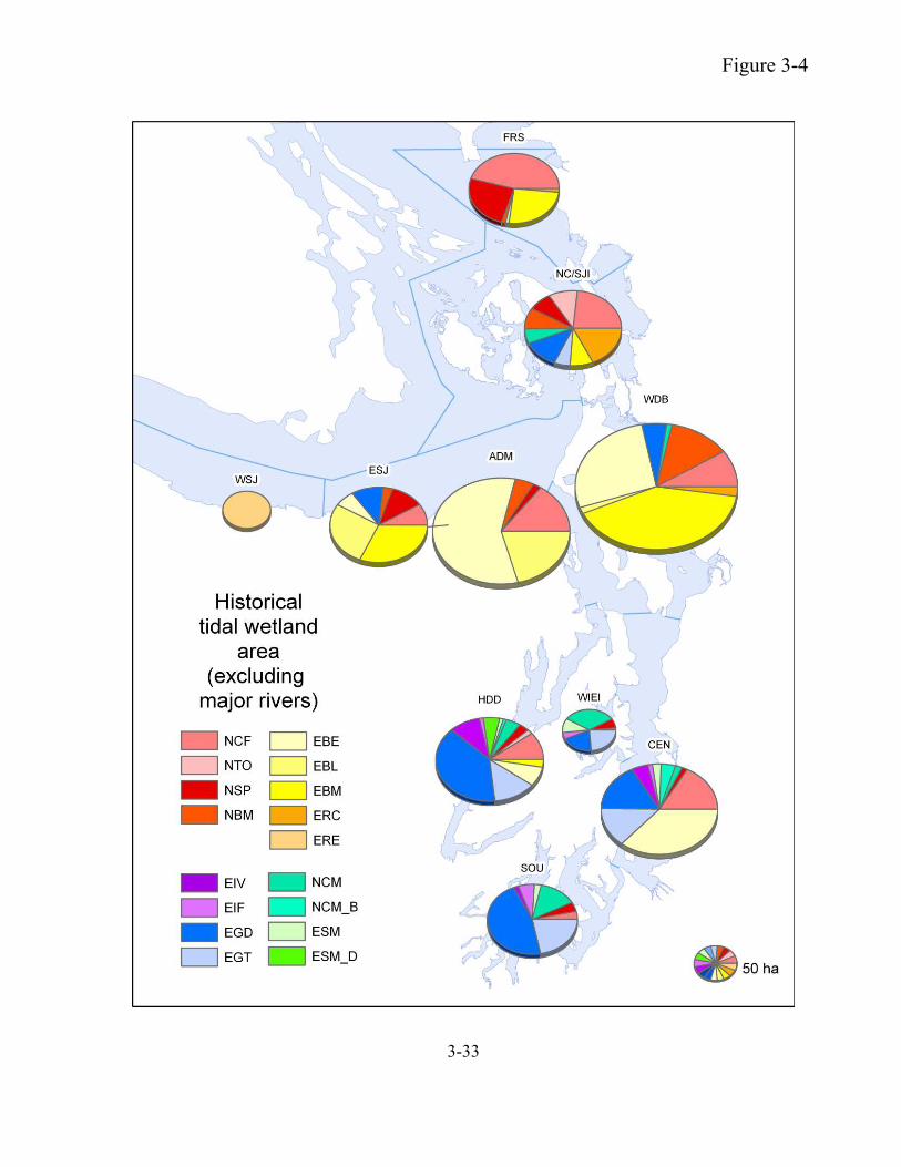
3-33

Figure 3-4

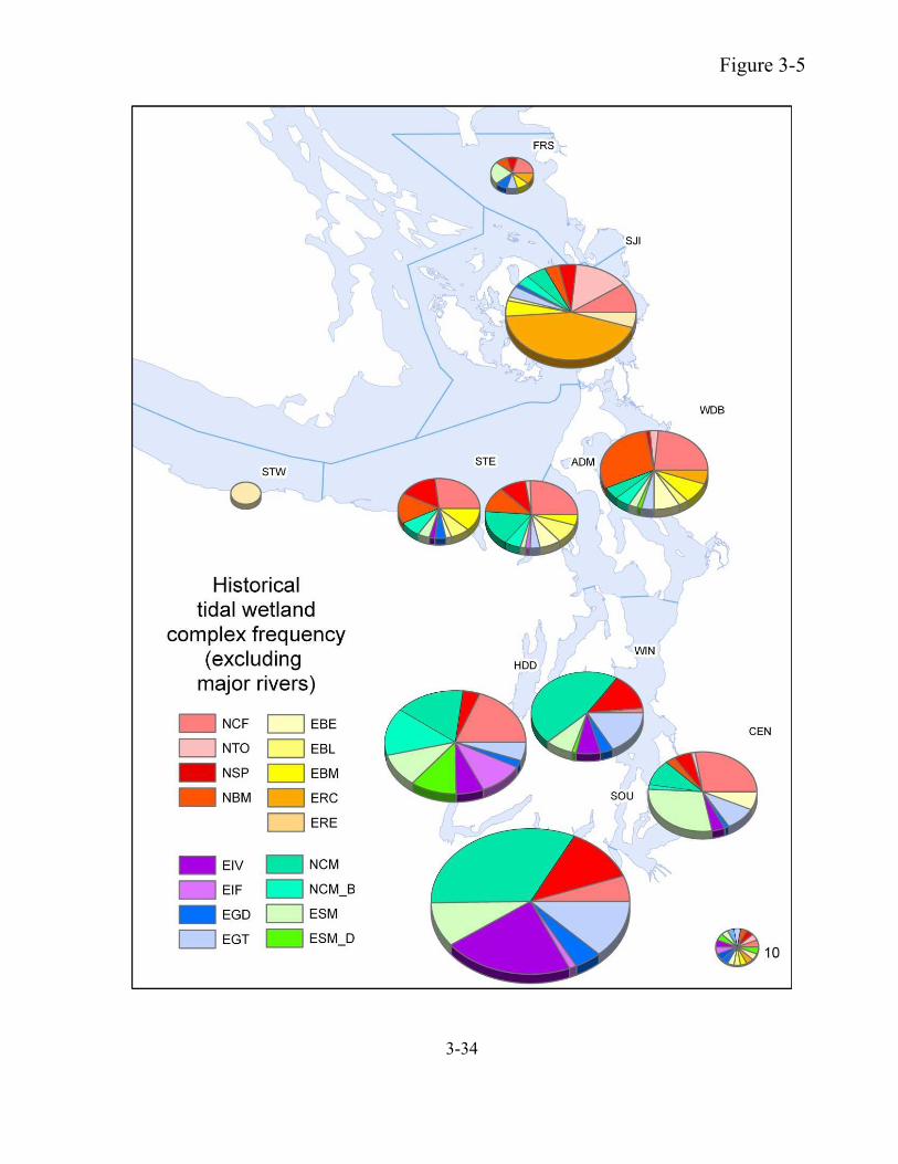
3-34

Figure 3-5

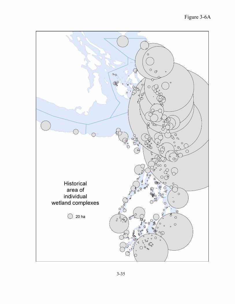
3-35

Figure 3-6A

3-36

Figure 3-6B

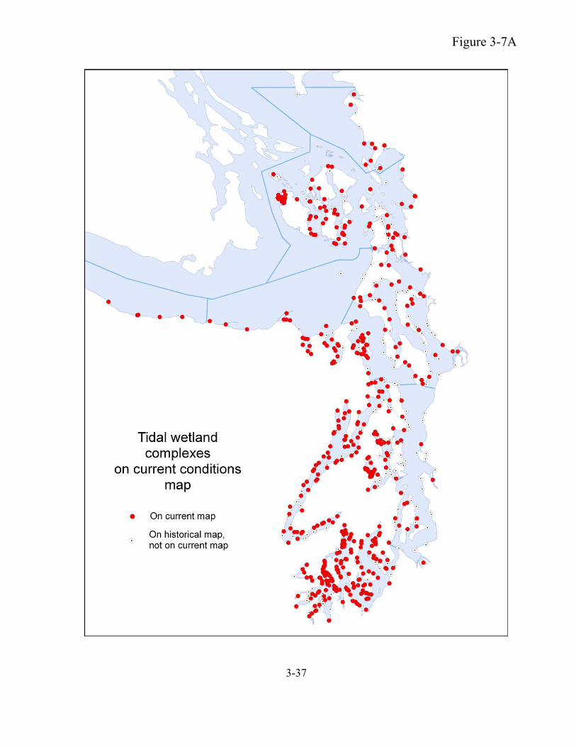
3-37

Figure 3-7A

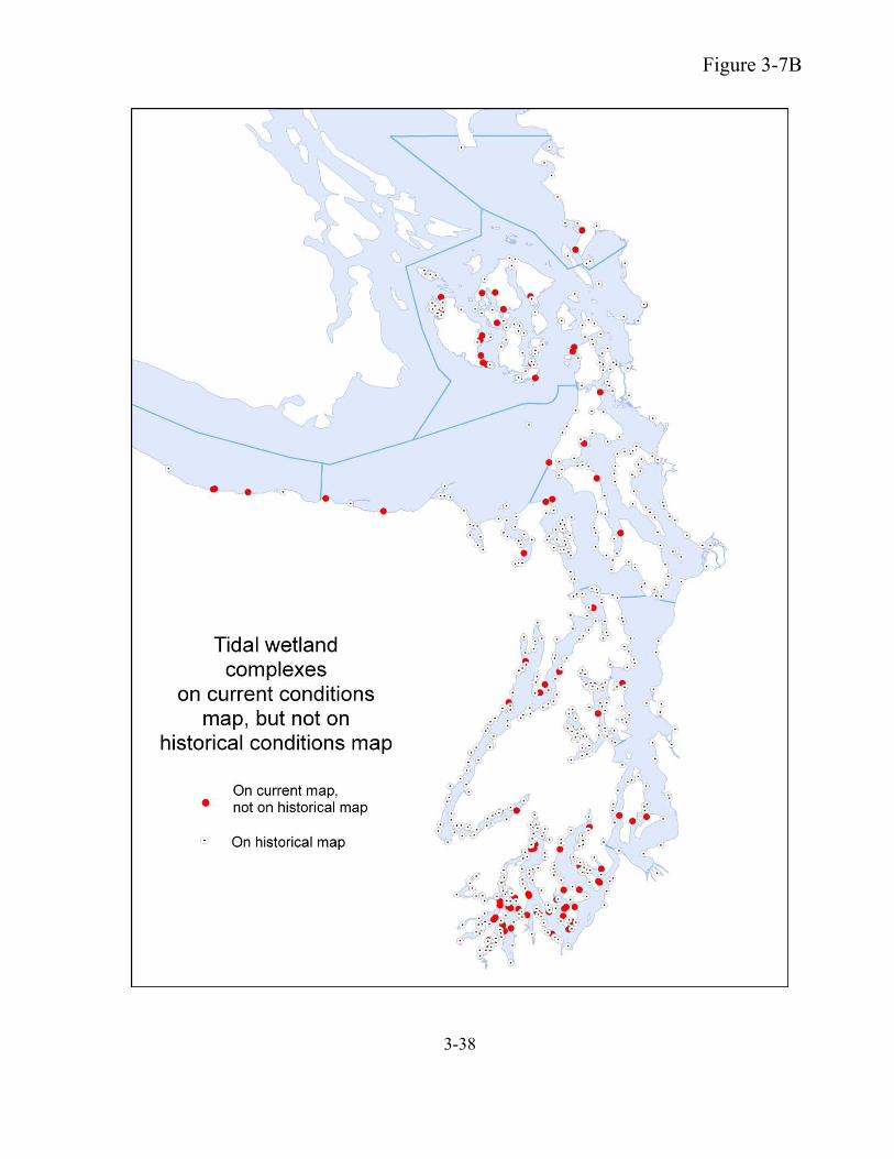
3-38

Figure 3-7B

3-39

Figure 3-8

A

B

3-40

Figure 3-9

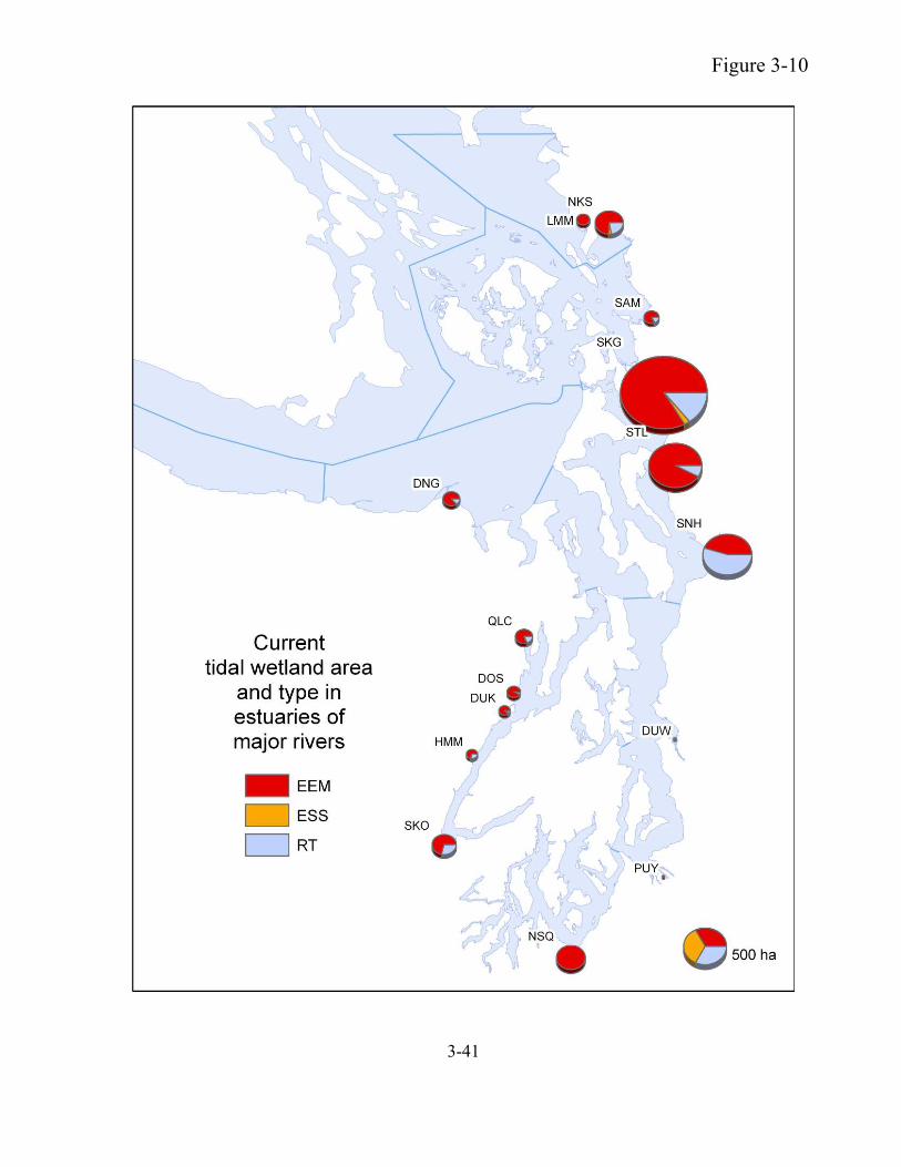
3-41

Figure 3-10

3-42

Figure 3-11

3-43

Figure 3-12A

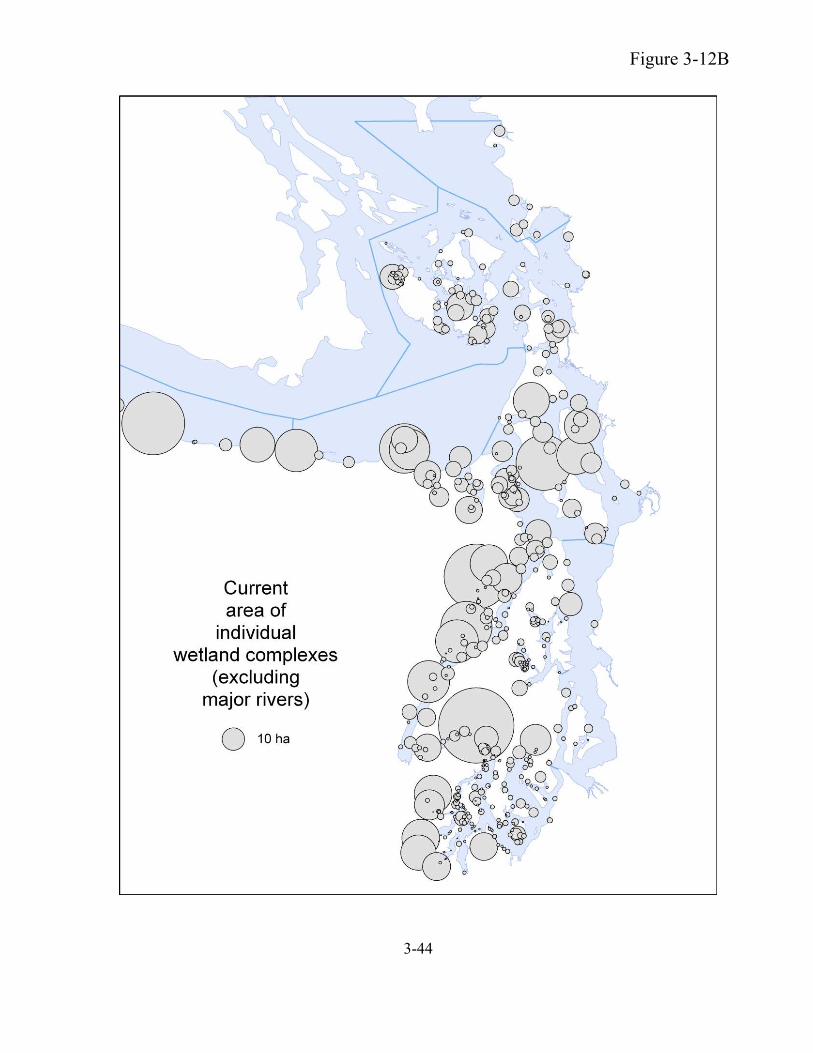
3-44

Figure 3-12B

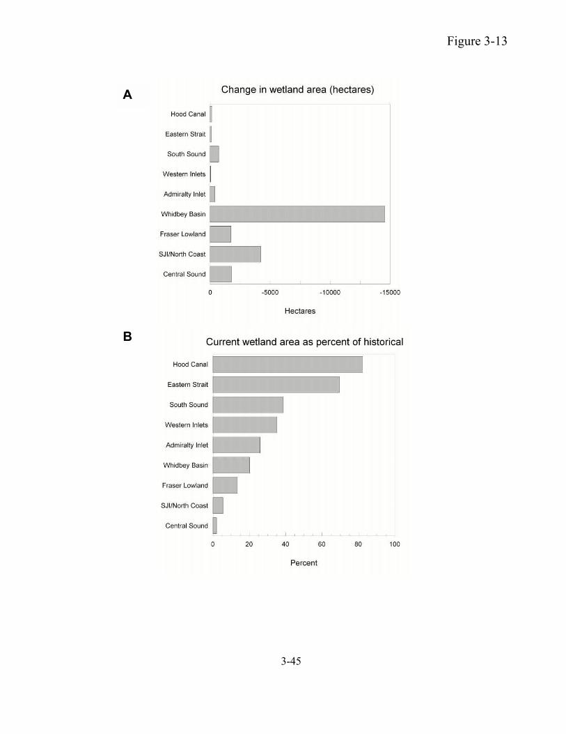
3-45

Figure 3-13

A

B

3-46

Figure 3-13

C

D

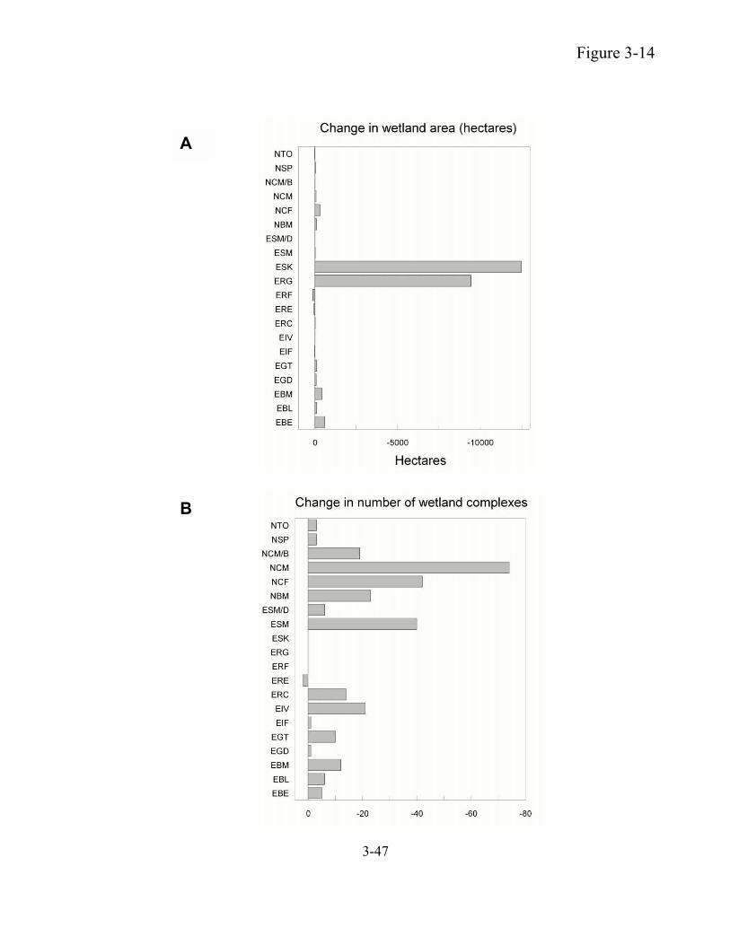
3-47

Figure 3-14

A

B

This project was funded by Washington DNR

Aquatic Resources Division

Washington State Department of Natural Resources

1111 Washington St SE, 1st floor

P.O. Box 47027

Olympia, WA 98504-7027

U.S.A.

(tel) 360.902.1100

http://www2.wadnr.gov/nearshore/

June 2005