Embed Size (px)
Citation preview

Hoang Nguyen Steven Martin
ECE 479: Intelligent Robotics II Human Facial Emotion Recognition Using OpenCV and Microsoft Kinect
Final Project Report

Nguyen and Martin 2
Table of Contents
1 INTRODUCTION ..............................................................................................................................................4
2 BACKGROUND .................................................................................................................................................4
2.1 OPENCV .......................................................................................................................................................4 2.2 UNIVERSALITY OF HUMAN EMOTIONS..........................................................................................................4 2.3 EMOTION RECOGNITION SYSTEM (ERS).......................................................................................................4
2.3.1 Principle Component Analysis (PCA)......................................................................................................5 2.3.2 Artificial Neural Networks (ANN) ...........................................................................................................5
3 FUNDAMENTALS AND IMPLEMENTATION OF PCA IN OPENCV .....................................................5
3.1 CALCULATING COVARIANCE MATRIX ...........................................................................................................7 3.2 FINDING EIGENVALUES AND EIGENVECTORS.................................................................................................7 3.3 THE MEANING OF EIGENVALUES AND EIGENVECTORS ...................................................................................9
4 PCA IN IMAGE COMPRESSION AND FEATURE EXTRACTION........................................................13
4.1 APPLYING PCA TO A SET OF FACE IMAGES ................................................................................................13 4.2 IMPLEMENTATION OF PCA IN OPENCV ......................................................................................................16
4.2.1 Introduction to Facial Expression Database .........................................................................................16 4.2.2 Apply PCA to the Facial Expression Database .....................................................................................17
5 NEURAL NETWORK TRAINING................................................................................................................20
6 KINECT INTERFACE ....................................................................................................................................23
7 FUTURE EXPANSIONS OF PROJECT .......................................................................................................27
8 PROJECT CONCLUSIONS............................................................................................................................27
APPENDIX A INSTALLING OPENCV AND OPENKINECT ......................................................................28
APPENDIX B PCA AND NN SOURCE CODE................................................................................................29
CFACERECOGNIZER.H ..............................................................................................................................................29 NEUNET.H ...............................................................................................................................................................29 CFACERECOGNIZER.CPP...........................................................................................................................................30 EMOREGBYANN.CPP ...............................................................................................................................................32
APPENDIX C KINECT INTERFACE SOURCE CODE ................................................................................38
MAKEFILE ................................................................................................................................................................38 KINECT.H..................................................................................................................................................................39 KINECTAPI.H.............................................................................................................................................................41 KINECT.CPP ..............................................................................................................................................................42 KINECTAPI.CPP .........................................................................................................................................................44
APPENDIX D WORKS CITED..........................................................................................................................47
APPENDIX E RELATED REFERENCES........................................................................................................47
Nguyen and Martin 3
List of Tables, Figures, and Equations
TABLE 1: A 2-DIMENSIONAL DATASET USED FOR DESCRIBING PCA...............................................................................6 EQUATION 1: FORMULA TO COMPUTE COVARIANCE MATRIX..........................................................................................7 TABLE 2: ALL COVARIANCE PARAMETERS OF 2-VARIABLE COVARIANCE MATRIX..........................................................7 EQUATION 2: DEFINITION OF EIGENVECTORS AND EIGENVALUES...................................................................................7 EQUATION 3: CHARACTERISTIC POLYNOMIAL OF A SQUARE MATRIX A .........................................................................8 TABLE 3: DATA VARIANCE FROM AVERAGE VALUES OF X AND Y................................................................................10 FIGURE 1: DATA VARIANCE FROM AVERAGE VALUES ..................................................................................................11 FIGURE 2: TWO EIGENVECTORS OF THE GIVEN DATASET ..............................................................................................12 FIGURE 3: SOME EXAMPLES OF EIGENFACES.................................................................................................................14 FIGURE 4: COMPUTE DATA MATRIX OF A DATABASE HAVING M IMAGES .....................................................................15 EQUATION 4: AVERAGE FACE FORMULA ......................................................................................................................15 EQUATION 5: SUBTRACTING IMAGE VECTORS BY AVERAGE VECTOR............................................................................15 EQUATION 6: COVARIANCE MATRIX C .........................................................................................................................15 EQUATION 7: FORMULA FOR IDENTIFYING EIGENFACES ...............................................................................................16 EQUATION 8: FORMULA FOR PROJECTING NEW IMAGE TO FACE-SPACE ........................................................................16 FIGURE 5: IMAGES FROM FACIAL EXPRESSION DATABASE ............................................................................................17 FIGURE 6: IMAGES FROM FACIAL EXPRESSION DATABASE ............................................................................................17 FIGURE 7: THE AVERAGE FACE COMPUTED FROM THE FACE MATRIX............................................................................18 FIGURE 8: THE FIRST SIX EIGENFACES COMPUTED FROM THE FACE MATRIX .................................................................19 FIGURE 9: A SET OF WEIGHT OBTAINED FROM PROJECTING AN IMAGE TO THE FACE-SPACE..........................................20 FIGURE 10: EXAMPLE ACTIVATION FUNCTION BASED ON SIGMOID..............................................................................21 FIGURE 11: BASIC ARCHITECTURE OF PCA CONNECTED TO BACK PROPAGATION NEURAL NETWORK ........................22 EQUATION 9: CHAIN RULE EXPANSION TO DERIVE LEARNING RULE...........................................................................23 EQUATION 10: DELTA LEARNING RULE .......................................................................................................................23 TABLE 4: PERFORMANCE COMPARISON BETWEEN DIFFERENT CHOICES OF HIDDEN LAYERS AND THE NUMBER OF
NEURONS IN THE HIDDEN LAYERS. .......................................................................................................................23 FIGURE 12: ARCHITECTURE OF KINECT INTERFACE, AND SUGGESTION FOR FUTURE EXPANSION. ................................25 TABLE 5: GENERALIZED OPENCV KINECT API............................................................................................................26

Nguyen and Martin 4
1 Introduction
The aim of this project is to use OpenCV and C++ to implement a facial expression recognition system that can be used in robotic applications. In a humanoid robot, the interaction between robot and people is critical. Therefore, integrating an emotion recognition system (ERS) into this kind of robot will make the interaction between robots and people more interesting and engaging.
An important point of implementing ERS in robots is real time processing of images taken from robots’ camera. Therefore, a fast processing algorithm would be more desirable in this project.
This project is implemented using OpenCV and C++ programming language. OpenCV is an open library for computer vision. More discussion about OpenCV and the reason of using it will be discussed in section 2 (Background).
2 Background
2.1 OpenCV
OpenCV is an Open Source Computer Vision library. It includes programming functions and more than 2500 optimized algorithms for real time computer vision. OpenCV has a large support community which is a great advantage for software development. At the moment of writing this report, OpenCV has C, C++ and Python interfaces and is available on Windows, Linux, Android and Mac.
Its main focus on real time processing (and portability) makes OpenCV an ideal choice for ERS instead of implementations done in programming languages such as MATLAB.
2.2 Universality of Human Emotions
Before going into details on understanding Emotion Recognition System, it is important to
know some basic facts about human emotions. Generally, there are 7 universal human
emotions: anger, disgust, happiness, sadness, fear, surprise and neutral. Dr. Paul Ekman [3]
mentions in his research that different cultures show the same facial expressions when
experiencing the same emotion unless culture-specific display rules interfere.
These 7 human emotions are recognized by Action Units which are groups of facial
muscles that when activated together result in a particular movement of facial features. For
example, an eyebrow being raised and a mouth being opened can describe a “surprised”
emotion.
2.3 Emotion Recognition System (ERS)
The emotion recognition system has been a significant field in human-computer interaction.
It is a considerably challenging field to generate an intelligent computer that is able to
identify and understand human emotions for various vital purposes, e.g. security, society, or
entertainment. Many research studies have been carried out in order to produce an
accurate and effective emotion recognition system. Emotion recognition methods can be
classified into different categories along a number of dimensions: speech emotion recognition
vs. facial emotion recognition; machine learning method vs. statistical method. Facial
expression method can also be classified based on input data consisting of a sequence video or

Nguyen and Martin 5
static images. This project will focus on recognizing emotions based on facial expression. The
main purpose of this project is to be applied in robotic application. Therefore, the ability to
analyze live video from a robot’s camera and distinguish different emotions is necessary. The
accuracy is not a critical purpose when weighed against other system performance, particularly
speed. (Real time, efficient, processing is much more important than 100% accuracy.)
The method used in this project for ERS is to combine Principle Component Analysis (PCA) with a Machine Learning algorithm - Artificial Neural Network (ANN).
ERS is separated into 2 phases: training phase and testing phase. In training phase, PCA is used for image compression and feature extraction. First, we need to apply PCA to a set of training images. The output of this PCA will be a set of feature weights (more detail is discussed in the section below). These sets of weights are the input of a Back Propagation Neural Network, which performs the task of machine learning. It will determine which specific features (and combinations of these features) best describe which specific emotions. In the testing phase, PCA is used to project a new image to a space defined by PCA for image compression. In this way, the PCA and ANN work together to develop a set of combined weights that can be used with real time video data.
2.3.1 Principle Component Analysis (PCA)
PCA was invented in 1901 by Karl Pearson [2]. It is a statistical approach which
compresses multi-variable data by identifying variance in the dataset and representing the data
in terms of this variance. This is achieved by building a covariance matrix and finding the
eigenvectors and eigenvalues of the covariance matrix. The covariance matrix identifies the
variance of the dataset. The eigenvector with the largest corresponding eigenvalue identifies
the greatest variance in the dataset. Each eigenvector contributes to identifying variance in the
dataset and is referred to as the principle component. This process allowed the interpretation of
complex dataset and became a popular tool in many fields of research. In image processing,
PCA is well-known for feature extraction and data compression.
Because of its ability for data compression, PCA significantly reduces computational requirements of the overall system. Therefore, it is an ideal choice to be integrated into real-time robotic applications; it reduces the original data to a minimal dataset that is still representative of the original data.
2.3.2 Artificial Neural Networks (ANN)
Artificial Neural Network is a machine learning algorithm that is based on biological neural networks (the biological brain). An ANN consists of interconnected groups of artificial neurons that can be represented in either hardware or software. ANN is an adaptive system that changes its structure based on external information that flows through the network during the learning phase. In image processing, neural network is used to obtain complex relationships between inputs and outputs to find particular pattern in data. In our context, we will be using the eigenvectors/eigenvalues produced during the PCA phase as inputs to the neural network, and the 7 emotions we are identifying will correspond to the outputs of the neural network.
3 Fundamentals and Implementation of PCA in OpenCV
The aim of this section is to explain the use of PCA in image compression by using a
simple example. We will go through all necessary steps to calculate principle components of a

Nguyen and Martin 6
given dataset. The next section will use a specific example in image processing to help readers
have a better understanding about PCA.
Let’s consider a 2-dimensional dataset as shown in the following table:
X Y
1 38
3 33
6 30
10 35
9 38
12 32
20 48
22 47
19 45
16 50
25 53
26 52
18 55
16 58
33 62
30 65
29 67
27 62
20 68
31 70
Table 1: A 2-dimensional dataset used for describing PCA
The preceding dataset is constructed in such a way that 2 variables have positive correlation.
Positive correlation means Y increases in respect to X generally.
Next step, the covariance matrix will be calculated from the table above.

Nguyen and Martin 7
3.1 Calculating covariance matrix
To find covariance matrix of a given dataset, the following formula is used to compute
covariance parameters in the matrix:
Equation 1: Formula to compute covariance matrix
A covariance matrix for 2-variable dataset will have following form:
Based on Equation 1, we can calculate all covariance parameters of the matrix as shown below:
cov(X,X) cov(X,Y) cov(Y,X) cov(Y,Y)
90.34 104.25 104.25 167.83
Table 2: All covariance parameters of 2-variable covariance matrix
One can see that covariance values of cov(X,Y) and cov(Y,X) are both positive. This
fact shows the positive correlation between X and Y as assumed from the beginning. If these
two values are negative, it shows that they have negative correlation which means one will
increase value when the other one decreases. One other case is when these two values are
both zero, there’s no correlation between these two variables.
From this example, it is apparent that the correlation between variables in a dataset can
be obtained by examining covariance matrix. This result is significant with a dataset having a
large number of variables. Applying this analysis for such system can show which variables
have the most effect in a system.
The next step to find principle components of the given dataset is to compute
eigenvalues and eigenvectors from the covariance matrix.
3.2 Finding eigenvalues and eigenvectors
Eigenvectors of a square matrix are the non-zero vectors that remain parallel to the
matrix after being multiplied by the matrix [4]. This definition can be briefly described by the
following expression:
Equation 2: Definition of eigenvectors and eigenvalues
In the equation: A is a square matrix, is eigenvalue and is eigenvector.
Eigenvalues and eigenvectors can be found by solving characteristic polynomial of the square
matrix A:

Nguyen and Martin 8
Equation 3: Characteristic polynomial of a square matrix A
In this particular example that we are considering, square matrix A is the covariance matrix, and
its characteristic polynomial is shown below:
Solve characteristic polynomial, we obtain 2 eigenvalues. It is possible, now, to find
eigenvectors of the covariance matrix.
In this example, square matrix A has the following form:
Eigenvectors for this matrix can be defined as:
With , eigenvector is found as:
This eigenvector can be normalized by the following method:

Nguyen and Martin 9
Therefore, normalized eigenvector is:
Similarly, normalized eigenvector is:
To summarize, the given dataset has 2 eigenvalues and 2 equivalent eigenvectors as following:
:
:
Eigenvalues and eigenvectors obtained from the covariance matrix will be used to identify data
patterns in the original dataset.
3.3 The meaning of eigenvalues and eigenvectors
In this section, we will discuss the practical meaning of eigenvalues and eigenvectors.
First of all, we will plot a diagram showing data variance of the given dataset from average
values.
X - Y -

Nguyen and Martin 10
-17.65 -12.4
-15.65 -17.4
-12.65 -20.4
-8.65 -15.4
-9.65 -12.4
-6.65 -18.4
1.35 -2.4
3.35 -3.4
0.35 -5.4
-2.65 -0.4
6.35 2.6
7.35 1.6
-0.65 4.6
-2.65 7.6
14.35 11.6
11.35 14.6
10.35 16.6
8.35 11.6
1.35 17.6
12.35 19.6
Table 3: Data variance from average values of X and Y

Nguyen and Martin 11
Figure 1: Data variance from average values
The eigenvectors of that dataset then will show the major trend of the variance in the following
plot.

Nguyen and Martin 12
Figure 2: Two eigenvectors of the given dataset
From the plot, we can see that the eigenvector with larger eigenvalue ( in this
case) express the major trend of data variance. And the second eigenvector shows the minor
trend of data variance from the average values of X and Y. These two eigenvectors are
perpendicular.
Each eigenvector is called principle component of a dataset. Eigenvector with largest
equivalent eigenvalue is called main principle component. With a given dataset, eigenvalues
need to be sorted from largest to smallest values. Eigenvectors then will be sorted in respect to
theirs corresponding eigenvalues. Principle component is perpendicular to each other. All
principle components of a dataset form an orthogonal space in which each principle component
is a coordinate.
With this example, two principle components help in identifying pattern in the dataset (how
much data vary from the mean and in which direction). Each principle component represents a
certain portion of the entire data. The number of principle components depends on the size of

Nguyen and Martin 13
covariance matrix. In this example, the covariance matrix is 2x2. Therefore, the maximum
number of principle components is 2.
4 PCA in Image Compression and Feature Extraction
In image processing, a dataset contains a lot of images. Each image is considered as a
‘point’ in a dataset. By applying PCA to that dataset, we can extract the features described by
the dataset. By projecting an image, which doesn’t belong to the given dataset, to an
orthogonal space formed by PCA, that image can be described as a point in the orthogonal
space. And its coordinates in the space express how much the image contains the features
described by the given dataset.
With a dataset with N images, the maximum number of principle components is N.
Projecting an image to the orthogonal space formed by PCA also results in decreasing data
needed to describe the image. For example, giving a dataset with 100 images, the maximum
number of principle components is 100. Therefore, the number of coordinates in orthogonal
space is also 100. A 150x150 image contains 22500 pixels. In the orthogonal space given by
the dataset, that image only needs 100 coordinates to be described correctly. Thus, PCA can
be used for image compression. The following section will discuss more detail how to apply
PCA to a set of face images.
4.1 Applying PCA to a Set of Face Images
One image can be converted into a vector by concatenating either the rows or the
columns of the image together. Applying this principle to all images in the set to create a matrix
with each image described by a row or column. This matrix then can be used to compute the
covariance matrix, eigenvectors (principle components) and eigenvalues of the set of images.
The eigenvectors are sorted by their corresponding eigenvalues. These principle components
describe the patterns in the dataset.
In the particular case of face images, all principle components form a space of faces (or
face-space). Each principle component contributes a certain amount of feature to represent the
face-space. In this situation, eigenvector is also called eigenface. These eigenfaces are called
“standardized face ingredients” [5]. With a large enough face database, any human face can be
considered as a combination of these standard faces by projecting that human face to face-
space. For example, one’s face can be composed of the average face plus 5% of eigenface 1,
20% of eigenface 2 and 60% of eigenface 3...

Nguyen and Martin 14
Figure 3: Some examples of eigenfaces
The following steps describe how to apply PCA to a set of face images theoretically. A specific
example will be given in the next section.
● Step 1 - Obtaining Grayscale image dataset: this step is not quite necessary because
many of available databases are grayscale. Also in this step, all images need to be
converted to a same size.
● Step 2 - Converting images into vectors: each image is converted to a column vector in
the dataset matrix . For example, a vector is obtained by resizing each NxN image
into a x1 vector. If there are M images in the database, the database matrix has
dimension of x .

Nguyen and Martin 15
Figure 4: Compute data matrix of a database having M images
● Step 3 - Compute Average Face: because each face is expressed as a vector in data
matrix, average face is also known as average vector. Average vector is computed by
the following formula:
Equation 4: Average face formula
Faces are generally similar and share many common features. By computing average
face and subtracting it from the faces in the database, we can remove the common
feature shared by all the faces. Using only the differences of each face results in a
better distribution of the face data, and also allows better feature extraction from the face
database.
● Step 4 - Subtract Average Vector from all vectors: to remove the common feature shared
by all face images, the original matrix is modified by subtracting individual column
vectors (images) by the average vector (average face).
Equation 5: Subtracting image vectors by average vector
is called mean-centered image.
● Step 5 - Generating the Covariance Matrix: the matrix is used to generate the
covariance matrix. The covariance matrix is found by the similar method used in the
example in section 3.1. The corresponding formula is given as following:
Equation 6: Covariance matrix C
● Step 6 - Compute Eigenvectors and Eigenvalues: eigenvectors and eigenvalues are
computed from the covariance matrix C. Detail calculation method is not listed here

Nguyen and Martin 16
because the main purpose of this paper is not about mathematics calculation. More
references about practical method to compute eigenvalues and eigenvectors are listed in
Appendix.
● Step 7 - Identifying Principle Components: computed eigenvalues are sorted from
largest to smallest values. Therefore, the corresponding eigenvectors are also sorted in
respect to theirs eigenvalues. These eigenvectors are principle components of the given
face database. Each principle component is perpendicular to each other, and together
form an orthogonal coordinate system.
● Step 8 - Calculating Eigenfaces: after eigenvectors have been sorted, they are multiplied
by the mean-centered images to generate eigenfaces. Therefore, each eigenvector
represents an eigenface which identifies a particular feature in the face-space. The
following equation is used to compute eigenfaces:
Equation 7: Formula for Identifying eigenfaces
In above equation, is principle components (eigenvectors) of the covariance matrix
identified by the given dataset.
The process of finding eigenfaces is also called feature extraction because eigenfaces
identify particular features described by the given face images.
● Step 9 - Projecting an image to face-space or Image Compression: each new image can
be converted into a set of weights (or coordinates in the orthogonal face-space) by being
projected onto the eigenfaces. This is obtained by applying the following equation:
Equation 8: Formula for projecting new image to face-space
with k = 1..M is the set of weights (or coordinates in the face-space) used to identify
the new image in the face-space. Generally, M is much smaller than the image size.
Therefore, the new image is compressed significantly by projecting it to the face-space.
The set of weights obtained from the projection also describes the features contained in the given image. For example, an image can be a combination of the average face plus 5% of eigenface 1, 20% of eigenface 2 and 60% of eigenface 3...
4.2 Implementation of PCA in OpenCV
In this section, a specific example will be given to illustrate the actual implementation of
PCA by OpenCV library.
4.2.1 Introduction to Facial Expression Database
One of the key factor to a successful ERS is a good and large enough facial expression
database. This is also an obstacle in this project because there are not so many available facial
databases. Some good databases as MMI face database and Cohn-Kanade Facial Expression
Database are available for research use but taking a great amount of time for their system to

Nguyen and Martin 17
grant access for students. Therefore, these databases are not included in this paper. However,
the result of this paper can be improved using databases from these sources when they are
available.
In this paper, we use JAFFE database (The Japanese Female Facial Expression
Database) and another database obtained from a paper about facial expression research [1].
Some of the images from these 2 databases are shown below.
Figure 5: Images from facial expression database
The number of images in the database is 97. All images are grayscale and converted to the
same size 150x150.
These images are classified to 7 categories corresponding to 7 emotions: happy, sad,
disgust, angry, surprise, fear and neutral.
4.2.2 Apply PCA to the Facial Expression Database
According to the steps mentioned in section 4.1, after obtaining grayscale images which
are already available in the database, all images are concatenated to form a matrix whose
columns are images in the database.
OpenCV library has PCA class that is designed specifically for PCA application.
Figure 6: Images from facial expression database

Nguyen and Martin 18
We apply this class to the matrix constructed by all the face images in the database. In
this matrix, images are converted to one column. Therefore, CV_PCA_DATA_AS_COL is
chosen as flag.
After applying this class to the matrix, it automatically computes the average vector,
subtracts all image vectors by this average vector, and compute eigenvectors and eigenvalues
from the mean-centered matrix. The following pictures are average face and some eigenfaces
computed by using PCA class in the matrix.
Figure 7: The average face computed from the face matrix

Nguyen and Martin 19
Figure 8: The first six eigenfaces computed from the face matrix
To describe any new image as a combination of eigenfaces, we need to project that
image to the face-space formed by all eigenvectors. There are 97 images in the training set.
Therefore, there are 97 eigenvectors or coordinates used to describe an image in the face-
space.

Nguyen and Martin 20
Figure 9: A set of weight obtained from projecting an image to the face-space.
As seen in the image above, an image projected to the face-space can be described as
a combination of 97 eigenvectors as following:
in which is the eigenvectors (or principle components) obtained from the face matrix. Any
image needs only 97 weights to be described in the face-space. These weights also express
the features contained in the image. For instance, the image used in this example has a large
number equivalent to eigenvector 2. That means it contains more features described by
eigenface 2. This example clearly shows the use of PCA in image compression and feature
extraction.
5 Neural Network Training
While Principle Component Analysis (PCA) can help find similarities between images, and
extract features from them, it doesn't necessarily mean that it can correctly determine which
emotion is present in the image. For example, an image in the “happy” training set may be
similar to another image in the “angry” set. Because of this, we may want images matching this
“happy” image to also suggest that the subject may be “angry” instead. Additionally, subset of
the “happy” faces, for example, may be more highly correlated to happiness than another, and
so it may be beneficial to weight the to give the stronger connections more weight in the
decision than the weaker connections.
One way to deal with these problems in a way that is compatible with the intention of the
original PCA technique is to pair the output vector produced by the PCA with a neural network
that is capable of learning these nuances in the data. This approach should result in a more
accurate prediction on emotion than can be achieved with PCA alone.
Neural networks are computation methods that are inspired by the biological brain and one
of its most fundamental building blocks: the neuron. In its overly simplistic form, an independent
neuron receives inputs from either a handful, or hundreds or thousands of neurons. Based on
the total sum of the inputs, the neuron will either fire, or will not fire, depending on if a threshold
is reached. Not all of the inputs to the neuron are equal, however. Some will weigh more
strongly on the outcome than others. Some will actually subtract from the total sum, instead of
adding to it. The output signal then propagates to other neurons, through both electrical and
chemical processes. Its impact on other neuron in the network are similarly weighted separately
to each neuron it is connected to.
This basic model of the neuron is what forms the basis of the back propagation neural
network, with some small changes. In this particular network, we have three layers of neurons,
or processing elements (PEs). The first (input) layer of PEs, in this case, comes directly from
the output of the PCA. The third, and final, layer is the output layer. Each PE in this layer
corresponds to one of the seven emotions that we are training the neural network to identify.
Nguyen and Martin 21
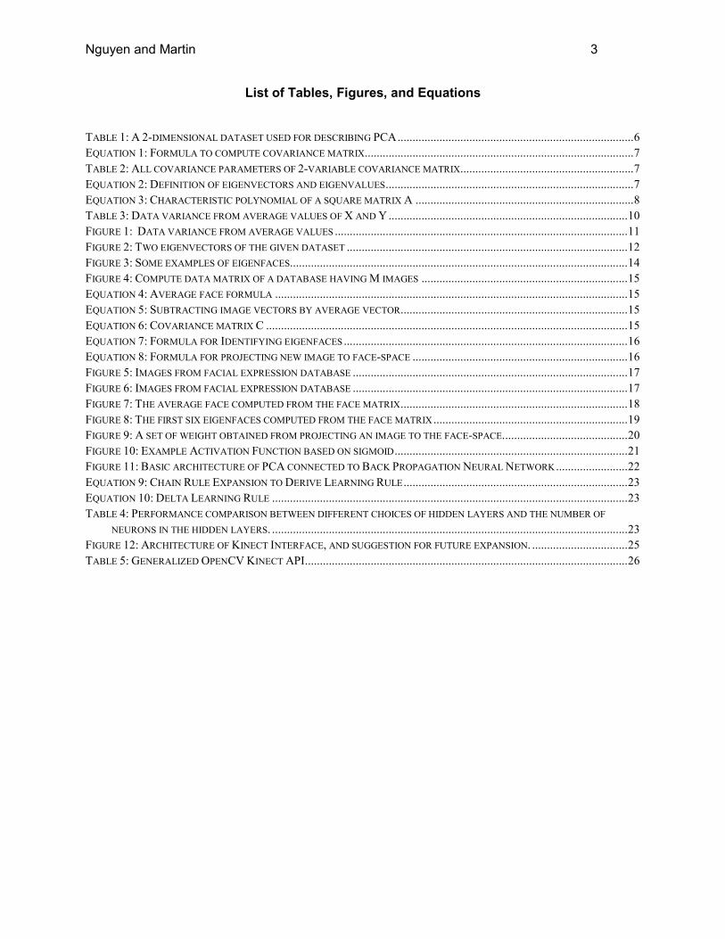
The middle layer, called the “hidden” layer, is the second stage of processing that allows
intermediate aspects of the analysis to be determined and stored, and therefore weighing on the
final output. Every PE at the input layer is connected to every PE of the hidden layer. Every PE
of the hidden layer is connected to every input at the output layer. At each stage, instead of an
all-or-nothing firing strategy, PEs in a back propagation network will instead fire using a sigmoid
function, so that low (or negative) values will result in an output close to -1 (or 0), and high
values will result in a value close to 1. Values in between will map to their corresponding
locations on the sigmoid curve. Each PE on the output will then fire with a magnitude of how
“sure” the neural network is that the face being identified matches the recognizable emotions.
The highest value is typically the response chosen, but the exact value may give any back end
system an indication on whether the results are accurate enough for further action based on the
results of the neural network analysis.
Figure 10: Example Activation Function based on sigmoid

Nguyen and Martin 22
Figure 11: Basic architecture of PCA connected to Back Propagation Neural Network
If we randomize all of the connection weights of the network (which is typically the starting
condition of most neural networks) passing an image through the PCA and then through the
neural network will, of course, yield random results. Adjusting the weights so that the neural
network yields expected results is called “training” the neural network. Training the network is
typically the first of two steps of getting a neural network to respond as expected, the second is
testing the neural network. Each step consists of running examples through the neural network,
however only in the “training” phase we will adjust the weights of the network to bring the
response closer to the expected value. We will run the “training” set hundreds, or even
thousands of times, depending on the data, and then validate against a separate set of data (the
“testing” set.) The reason for using separate data is to guarantee that the neural network
trained the weights such that it is capable of interpreting data that it has never seen before
(generalized learning), as opposed to simply “memorizing” the patterns it was trained on.
After each training example is presented to the neural network, the weights are adjusted
such that the overall error of the response is reduced. Adjusting the weights between the
hidden PEs and the output PEs is fairly straightforward. Simplified, we adjust each weight to
each output by the error value (typically the square of the difference between the expected (1 if
the emotion is expected, 0 if not), and actual value.) This error value is multiplied by the
previous weight, because this is the proportion that this particular connection contributed to the
error.
The reason we use the derivative to find the proper signal to change the weights may, at
first, not be immediately clear. What we are attempting to do is calculate the weight change that
will bring us closer to the weight value that reduces the error function as much as possible. To
do this, we use derivative which will give us a rate of change of the function as compared to the
weight in question. In other words, we operate “as if” the weight change will follow a gradient
descent to reduce the overall error. From Haykin’s book “Neural Networks and Learning
Machines”, we know that this rate of change can be expressed by calculus chain rule
expansion as [6]:
Nguyen and Martin 23
( )( )
( )( )
( )
( )
( )
( )
( )
( )nw
nv
nv
ny
ny
ne
ne
n
nw
n
ji
j
j
j
j
j
jji ∂
∂
∂
∂
∂
∂
∂
∂=
∂
∂ εε
Equation 9: Chain Rule Expansion to Derive Learning Rule
Where ε is the error function, jiw is the weight from neuron i to j, je is the expected output after
summation and activation function into the node, jy is the actual output, and jv is the actual
summation at neuron j.
After differentiating, and adding a learning rate coefficient, we end up with:
( ) ( ) )()( nynvnew ijjjji
′=∆ ϕη
Equation 10: Delta Learning Rule
Where η is our learning coefficient (parameterized depending on problem), and ( ))(nv jj
′ϕ
is the derivative of the activation function.
Number of hidden layers
Layer 1
Layer 2
Results
2 10 20 Obtain good results, known images close to what expected. Unknown images are predicted closely to final results.
1 5 Works good compared to previous results. Besides, using only one layer improves the processing speed.
1 20 The results obtained are about the same as using 5 neutrons in the hidden layer but the processing speed increases.
Table 4: Performance comparison between different choices of hidden layers and the number of
neurons in the hidden layers.
As seen in the table above, we get good results using of only 1 hidden layer with 5 neurons.
Keep increasing the number of layers or neurons doesn’t have a significant impact on the final
result but increasing the processing time. Therefore, we decided to use 1 hidden layer with 5
neurons in our neural network.
6 Kinect Interface

Nguyen and Martin 24
One of the challenges of the project was successfully interfacing with a Kinect Camera to
gather frame information. What makes this a challenge is the fact that many parts of the final
robotic system will need access to the same camera interface. The goal of the Kinect Interface
code is to create an Application Programming Interface (API) that interfaces directly with the
Kinect that could eventually by wrapped in an identical API that accesses the Kinect over a
small LAN network (or network switch.) The idea behind this is creating a stable layer that does
not eat a lot of system resources to get camera information, but is also thread-safe so that
multiple programs can access the same resources, as well as prevent direct access to the
camera, which helps keep the system stable by providing a single-point of entry to get access to
the Kinect camera information (both the RGB video, as well as the depth information provided
by the camera.)
An added benefit of this approach is that it frees up anyone who need to interface with the
Kinect for future projects from having to develop code to access the device. Instead, they can
simply call tested API calls that will abstract away implementation details, and easily yield
OpenCV Mat data classes so that they can be easily manipulated from within the OpenCV
framework.
The underlying architecture is a set of circular buffers. One buffer is for the RGB frame
data from the Kinect, and the other is the depth image. (Only one buffer is shown in the
diagram for clarity.) The depth image is simply a grayscale image, however, each pixel’s value
is representative of how far an object is from the Kinect, rather than information about its
spectral characteristics. Whenever a new frame is available from the Kinect hardware, the
program is interrupted to add another frame to the buffer after checking that the frame is no
longer in use. Whenever a subsystem of the robot requires a new frame, the newest frame is
given to them, but the buffer location is locked (except to other subsystems) until the frame has
been successfully copied out.
The current number of frames in the buffer is 10, although this can be modified when the
source code is compiled. (It is unlikely that the oldest frame will be in use when the Kinect has
a new frame available, but synchronization is still required to prevent system crashes in the rare
case that it does happen.)

Nguyen and Martin 25
kinect.cpp:
Provides thread-safe interaction with libfreenect layer, so that frame information can be
retrieved in an efficient manner for any subsystem requiring.
libfreenect:
Open Source library that
configures callbacks so that
client program will be notified
whenever new Kinect frames
are available.
kinectapi.cpp:
Provides simple access to
Kinect device, as well as
conversion to various OpenCV
Mat formats (grayscale, rgb,
depth information, etc.)
Unified Network Layer for
Entire Robot System:
(Not implemented in time for
this project)
Kinect Net:
Built on top of network layer. This
layer will have the exact API
commands as kinectapi.cpp. In
other words, it mimics as though
the Kinect is directly attached, but
actually connects to the frame
data using networking commands.
FRAME
FRAME
FRAME
FRAME
FRAME
FRAME
When new frame is
available, kinect.cpp
copies new frame,
ensuring frame is not
being accessed
Newest frame is always
copied when
requested. Frame data
is temporarily locked
until whatever thread
requesting data is
satisified.
Circular Buffer
Circular Buffer ensures
that there is always room
to copy in a new frame
(asynchronous callback),
but any frame that is
currently being copied
does not get corrupted
before copy is
completed.
Kinect Server:
Built on top of network layer. This
layer uses the kinectapi base code
to create a server service that
allows multiple Kinect Clients to
get frame data over the network
Figure 12: Architecture of Kinect Interface, and suggestion for future expansion.
To use the interface, you simply need to include the kinectapi.h header file, and then
create a kinectinterface object.
kinectinterface interface();

Nguyen and Martin 26
Then, you can use the following API commands to get the latest frame images. For example,
you can get a 8-bit grayscale video image by doing the following:
Mat * gray8 = interface.get8BitGrayscale();
The interfacing routines to get OpenCV matrices from the Kinect are written in a way that
abstracts away the implementation details. This was done to allow these APIs to be ported to
other system configurations. In particular, it was written to allow multiple systems to connect to
a server that feeds out frame information to these devices. This can be implemented by writing
a server, that will be written for an underlying network layer, that accesses the Kinect directly
using the kinectapi source code (Kinect Server). This will allow devices to connect to it, and
then feed frame data over the network as required. In this way, the only program getting access
to the Kinect directly is the Kinect Server. Other devices can then use code that has an
identical API to the kinectapi code, but then are wrappers for communication with the Kinect
Server. The end goal of this would be to allow programs to run identically regardless of whether
the Kinect was directly attached, or if the Kinect was actually connected to an entirely different
device.
API Call Description
Mat * get8BitRGB(); Return a pointer to the latest RGB frame (8 bits per color)
available from the Kinect. The pointer is valid until get8BitRGB()
is called again.
Mat * get16BitDepth(); Return a pointer to the latest depth frame, w/ 16 bits of
information per pixel. The pointer is valid until get16BitDepth()
is called again.
Mat * get8BitDepth(); Return a pointer to the latest depth frame, w/ 8 bits of
information per pixel. The pointer is valid until get8BitDepth() is
called again.
Mat * get8BitGrayscale(); Return a pointer to the latest video frame (8 bits grayscale
information per pixel) available from the Kinect. The pointer is
valid until get8BitGrayscale () is called again.
Mat * get16BitGrayscale(); Return a pointer to the latest video frame (16 bits grayscale
information per pixel) available from the Kinect. The pointer is
valid until get16BitGrayscale () is called again.
uint32_t
getLastTimestamp();
Get the timestamp from the very last function get* function
called
int getLastFrameNum(); Get the frame count number from the very last function get*
function called. NOTE: It is possible for depth and video frames
to drift slightly from each other on a running system.
Table 5: Generalized OpenCV Kinect API

Nguyen and Martin 27
7 Future Expansions of Project
While much was done this term, there is still lots of room for future expansion of this project.
First of all, the larger the dataset of human face images that are available, the more accurate
the algorithm could be. As of the writing of this report, the images available were very limited,
and we were unable to get access to the larger databases available for academia with enough
time to use them in our algorithm. Once these new images are obtained, it would then be
possible to further tune the neural network portion of the algorithm. We can adjust the learning
coefficient of the system, the momentum terms, number of hidden nodes, number of training
iterations, etc., until we find the weights that lead to the most accurate emotion recognition.
Once this is done, we can save the weights so that the neural network does not have to be
retrained during operating mode.
Another place with room for expansion is the Kinect interface. The networking layer that
will be available to all components of the final robotic system was not ready in time for a Kinect
Server and Kinect Client software to be written. These components would be relatively quick to
develop and implement, and could produce a backbone for any component in the final system
that requires image information (video or depth) from the Kinect in a manner that improves
overall system stability.
Additionally, it might be possible to use the depth information in parallel with the video
frame information in emotion recognition. If a database of depth image faces could be
produced, it might be possible to implement the PCA algorithm on the new dataset, and have
these be additional inputs to the NN for training and operation mode.
8 Project Conclusions
By the end of this project, a system that could read data from the Kinect, and then
recognize human emotion characteristics was created. There is much room form improvement
when larger emotion test sets are introduced, and potentially there is room for improvement if
depth images are introduced to the PCA algorithm, so that more information can be used to
characterize a person’s facial expressions to determine emotion.
The PCA algorithm seemed to work really well, and very quickly, to extract elements of
people’s faces to determine an emotion set. Using live camera data, it recognized easy
emotions such as “happiness”, when we smiled into the camera. The neural network was very
efficient as well, despite the fact that more training/tuning may be required once the test set is
expanded.
While much work is required to make the solution more robust, and ready to be
implemented in a live robotic system, much of the heavy lifting has been done, and the
framework has been laid for future students to take on this project, expand it, refine it, and then
finally implement it.

Nguyen and Martin 28
Appendix A Installing OpenCV and OpenKinect
OpenCV, and libfreenect, can easily be installed on a Ubuntu system. Please note that these
instructions are for OpenCV version 2.1 on a Ubuntu 11.10 system. This is the version of
OpenCV that is considered stable by Ubuntu, as of this writing, and is checked into the Ubuntu
distribution system. Version 2.3 is also available, but the installation instructions are not as
simple, and are not covered here. The source code for this project should work with OpenCV
version 2.3, but this compatibility is not guaranteed—some minor porting may be required. Also
note that the libfreenect installation instructions may change. Please visit www.openkinect.org
for the latest installation instructions.
To install OpenCV 2.1 on a Ubuntu machine, simply type the following command (one line):
sudo apt-get install libcv-dev libcv2.1 libcvaux-dev libcvaux2.1 libhighgui-dev libhighgui2.1
Libfreenect, the library used to interface with the camera, can be installed using the following
commands:
sudo add-apt-repository ppa:floe/libtisch sudo apt-get update sudo apt-get install libfreenect libfreenect-dev libfreenect-demos sudo adduser $USER video

Nguyen and Martin 29
Appendix B PCA and NN Source Code
cFaceRecognizer.h #ifndef __FACERECOGNIZER_H__ #define __FACERECOGNIZER_H__ #include <iostream> #include <vector> #include <float.h> #include <cv.h> using namespace std; using namespace cv; class FaceRecognizer { public: FaceRecognizer(const Mat& trFaces, const vector<int>& trImageIDToSubjectIDMap); ~FaceRecognizer(); void init(const Mat& trFaces, const vector<int>& trImageIDToSubjectIDMap); int recognize(const Mat& instance); Mat getWeight(const Mat& testImage); Mat getAverage(); Mat getEigenvectors(); Mat getEigenvalues(); private: PCA *pca; vector<Mat> projTrFaces; vector<int> trImageIDToSubjectIDMap; }; #endif
NeuNet.h /* * NeuNet.h * * Created on: Feb 7, 2012 * Author: hoang */ #ifndef NEUNET_H_ #define NEUNET_H_ #include <opencv2/core/core.hpp> #include <opencv2/highgui/highgui.hpp> //required for multilayer perceptrons #include<opencv2/ml/ml.hpp> using namespace cv; class cANN { public: CvANN_MLP ann; void trANN(const Mat& trainingData, const Mat& trainingResults) // Traing the Neural Net

Nguyen and Martin 30
{ cv::Mat layers = cv::Mat(3, 1, CV_32SC1); //create 3 layers layers.row(0) = cv::Scalar(trainingData.cols); //input layer accepts the weights of input images layers.row(1) = cv::Scalar(5);//hidden layer //layers.row(2) = cv::Scalar(10);//hidden layer layers.row(2) = cv::Scalar(7); //output layer returns to one of 7 emotions //ANN criteria for termination CvTermCriteria criter; criter.max_iter = 200; // *********change 100 to 200 for experiment*********** criter.epsilon = 0.00001f; criter.type = CV_TERMCRIT_ITER | CV_TERMCRIT_EPS; //ANN parameters CvANN_MLP_TrainParams params; params.train_method = CvANN_MLP_TrainParams::BACKPROP; params.bp_dw_scale = 0.05f; params.bp_moment_scale = 0.05f; params.term_crit = criter; //termination criteria ann.create(layers); // train ann.train(trainingData, trainingResults, cv::Mat(), cv::Mat(), params); } Mat teANN(const Mat& testingData) { Mat predicted(testingData.rows, 7, CV_32FC1); // Row is the number of testing images, Column is emotions recognized for(int i = 0; i < testingData.rows; i++) { Mat response = predicted.row(i); Mat sample = testingData.row(i); ann.predict(sample, response); } // std::cout << predicted << std::endl; return predicted; } }; #endif /* NEUNET_H_ */
cFaceRecognizer.cpp #include "cFaceRecongizer.h" FaceRecognizer::FaceRecognizer(const Mat& trFaces, const vector<int>& trImageIDToSubjectIDMap) { init(trFaces, trImageIDToSubjectIDMap); } void FaceRecognizer::init(const Mat& trFaces, const vector<int>& trImageIDToSubjectIDMap) {

Nguyen and Martin 31
int numSamples = trFaces.cols; this->pca = new PCA(trFaces, Mat(),CV_PCA_DATA_AS_COL); for(int sampleIdx = 0; sampleIdx < numSamples; sampleIdx++) { this->projTrFaces.push_back(pca->project(trFaces.col(sampleIdx))); } this->trImageIDToSubjectIDMap = trImageIDToSubjectIDMap; } FaceRecognizer::~FaceRecognizer() { delete pca; } int FaceRecognizer::recognize(const Mat& unknown) { // Take the vector representation of unknown's face image and project it // into face space. Mat unkProjected = pca->project(unknown); // I now want to know which individual in my training data set has the shortest distance // to unknown. double closestFaceDist = DBL_MAX; int closestFaceID = -1; for(unsigned int i = 0; i < projTrFaces.size(); i++) { // Given two vectors and the NORM_L2 type ID the norm function computes the Euclidean distance: // dist(SRC1,SRC2) = SQRT(SUM(SRC1(I) - SRC2(I))^2) // between the projections of the current training face and unknown. Mat src1 = projTrFaces[i]; Mat src2 = unkProjected; double dist = norm(src1, src2, NORM_L2); // Every time I find somebody with a shorter distance I save the distance, map his // index number to his actual ID in the set of traing images and save the actual ID. if(dist < closestFaceDist) { closestFaceDist = dist; closestFaceID = this->trImageIDToSubjectIDMap[i]; } } return closestFaceID; } // Project a test image to face-space and get its weight Mat FaceRecognizer::getWeight(const Mat& testImage) { return pca->project(testImage); } // Returns the vector containing the average face. Mat FaceRecognizer::getAverage() { return pca->mean; } // Returns a matrix containing the eigenfaces. Mat FaceRecognizer::getEigenvectors() {

Nguyen and Martin 32
return pca->eigenvectors; } // Returns a matrix containing the eigenvalues. Mat FaceRecognizer::getEigenvalues() { return pca->eigenvalues; }
EmoRegByAnn.cpp #include <cv.h> #include <highgui.h> #include "objdetect/objdetect.hpp" #include "imgproc/imgproc.hpp" #include "highgui/highgui.hpp" #include <iostream> #include <sstream> #include <fstream> #include <string> #include <vector> #include "cFaceRecongizer.h" #include "NeuNet.h" //#include "kinectapi.h" using namespace std; using namespace cv; // Test lists consist of the subject ID of the person of whom a face image is and the // path to that image. void readFile(const string& fileName, vector<string>& files, vector<int>& indexNumToSubjectIDMap) { while (!files.empty()) { files.pop_back(); // empty this vector before adding anything to it, // to make sure there's no repetitive info in this vector } std::ifstream file(fileName.c_str(), ifstream::in); if(!file) { cerr << "Unable to open file: " << fileName << endl; exit(0); } std::string line, path, trueSubjectID; while (std::getline(file, line)) { std::stringstream liness(line); std::getline(liness, trueSubjectID, ';'); std::getline(liness, path); path.erase(std::remove(path.begin(), path.end(), '\r'), path.end()); path.erase(std::remove(path.begin(), path.end(), '\n'), path.end()); path.erase(std::remove(path.begin(), path.end(), ' '), path.end());

Nguyen and Martin 33
files.push_back(path); indexNumToSubjectIDMap.push_back(atoi(trueSubjectID.c_str())); } } void unableToLoad() { cerr << "Unable to load face images. The program expects a set of face images in a subdirectory" << endl; cerr << "of the execution directory named 'att_faces'. This face database can be freely downloaded " << endl; cerr << "from the Cambridge University Copmputer Lab's website:" << endl; cerr << " http://www.cl.cam.ac.uk/research/dtg/attarchive/facedatabase.html" << endl; exit(1); } int main(int argc, char *argv[]) { // Defining variables vector<string> teFaceFiles; vector<int> teImageIDToSubjectIDMap; vector<string> trFaceFiles; vector<int> trImageIDToSubjectIDMap; double duration1(0), duration2(0), duration3(0); // These variables used to evaluate the performace of PCA and NN string trainingList = "./train_original.txt"; string testList = "./test_original.txt"; string face_cascade_name = "haarcascade_frontalface_alt.xml"; // Cascade classifier used for face tracking CascadeClassifier face_cascade; // Define an instance of class face_cascade used for tracking face if( !face_cascade.load( face_cascade_name ) ) // Load Cascade classifier { printf("--(!)Error loading\n"); return -1; }; // Read training dataset readFile(trainingList, trFaceFiles, trImageIDToSubjectIDMap); Mat teImg = imread(trFaceFiles[0], 0); Mat trImg = imread(trFaceFiles[0], 0); if(trImg.empty()) { unableToLoad(); } // Eigenfaces operates on a vector representation of the image so we calculate the // size of this vector. Now we read the face images and reshape them into vectors // for the face recognizer to operate on. int imgVectorSize = teImg.cols * teImg.rows;

Nguyen and Martin 34
// Create a matrix that has 'imgVectorSize' rows and as many columns as there are images. Mat trImgVectors(imgVectorSize, trFaceFiles.size(), CV_32FC1); // Load the vector. for(unsigned int i = 0; i < trFaceFiles.size(); i++) { Mat tmpTrImgVector = trImgVectors.col(i); Mat tmp_img; imread(trFaceFiles[i], 0).convertTo(tmp_img, CV_32FC1); tmp_img.reshape(1, imgVectorSize).copyTo(tmpTrImgVector); } //******************************Training phase**************************************** // On instantiating the FaceRecognizer object automatically processes // the training images and projects them. // Evaluate the time needed for PCA implementation duration1 = static_cast<double>(cv::getTickCount()); FaceRecognizer fr(trImgVectors, trImageIDToSubjectIDMap); duration1 = static_cast<double>(cv::getTickCount()) - duration1; duration1 /= cv::getTickFrequency(); /////////////Initialize Input Layer for Neural Network///////////////////// // Loop through all training images and get the weights of each of them; // Put these weights into a Matrix used for training Neural Network // Evaluate the time needed for training NN duration2 = static_cast<double>(cv::getTickCount()); Mat temp; trImg.convertTo(temp, CV_32FC1); Mat weight_temp = fr.getWeight(temp.reshape(1, imgVectorSize)); // The weights of each image is described in one row instead of column Mat trainingData(trFaceFiles.size(), weight_temp.rows, CV_32FC1, Scalar::all(0)); // Initialize a Matrix to store all training weights for (unsigned int i=0; i<trFaceFiles.size(); i++) { Mat temp = trainingData.row(i); Mat temp1; imread(trFaceFiles[i],0).convertTo(temp1, CV_32FC1); Mat weight_temp = fr.getWeight(temp1.reshape(1, imgVectorSize)); weight_temp.reshape(1, 1).copyTo(temp); // Change the format of the weight so it can fit in one traingData row } //////////Initialize Output Layer for Neural Network///////////////// Mat trainingResults(trFaceFiles.size(), 7, CV_32FC1, Scalar::all(0)); // Row is the number of training images, // Column is equivalent 7 emotions for (unsigned int i=0; i < trFaceFiles.size(); i++) { switch(trImageIDToSubjectIDMap[i]) { case 1: // Sad trainingResults.at<float>(i,0) = 1; break; case 2: // Angry trainingResults.at<float>(i,1) = 1; break;

Nguyen and Martin 35
case 3: // Digust trainingResults.at<float>(i,2) = 1; break; case 4: // Neutral trainingResults.at<float>(i,3) = 1; break; case 5: // Fear trainingResults.at<float>(i,4) = 1; break; case 6: // Surprise trainingResults.at<float>(i,5) = 1; break; case 7: // Happy trainingResults.at<float>(i,6) = 1; break; } } // Implement Neural Network cANN emoANN; // Train the NeuralNet with trainingData and trainingResults emoANN.trANN(trainingData, trainingResults); duration2 = static_cast<double>(cv::getTickCount()) - duration2; duration2 /= cv::getTickFrequency(); cout << "Training complete!!!" << endl; //****************************Testing phase********************************// // Use Neural Network to evaluate the testing image // Initialize a Matrix to store all weights of test images //kinectinterface interface; // an instace of kinect interface, used to capture frames from kinect, uncomment this to capture image from Kinect //Mat* grayimg; CvCapture* capture; Mat frame, gray_frame; capture = cvCaptureFromCAM( -1 ); while (1) { // Evaluate time needed for testing an image using NN // readFile(testList, teFaceFiles, teImageIDToSubjectIDMap); // duration3 = static_cast<double>(cv::getTickCount()); /* This part is used to test individual images */ // Mat testingData(teFaceFiles.size(), weight_temp.rows, CV_32FC1, Scalar::all(0)); // for (unsigned int i=0; i<teFaceFiles.size(); i++) // { // Mat temp = testingData.row(i); // Mat temp1; // imread(teFaceFiles[i],0).convertTo(temp1, CV_32FC1); // Mat weight_temp = fr.getWeight(temp1.reshape(1, imgVectorSize)); // weight_temp.reshape(1, 1).copyTo(temp); // Change the format of the weight so it can fit in one traingData row // } // Testing an image captured from Kinect, uncomment this to capture frame from Kinect // grayimg = interface.get8BitGrayscale(); // Mat gray_frame = *grayimg;
Nguyen and Martin 36
// Testing an image captured from normal video frame = cvQueryFrame( capture ); cvtColor( frame, gray_frame, CV_BGR2GRAY ); equalizeHist( gray_frame, gray_frame ); // Face tracking using face cascade classifier vector<Rect> faces; // define a vector to contain faces info from Face tracking classifier face_cascade.detectMultiScale( gray_frame, faces, 1.1, 2, 0|CV_HAAR_SCALE_IMAGE, Size(100, 100) ); for (int i = 0; i<faces.size(); i++) { Point top_left(faces[i].x, faces[i].y + 20); Point top_right(faces[i].x + faces[i].width, faces[i].y + faces[i].height + 20); rectangle(gray_frame, top_left, top_right, Scalar( 255, 0, 255 )); Mat faceROI = gray_frame(Rect(faces[i].x, faces[i].y+20, faces[i].width , faces[i].height)); // define Region of Interest Mat faceROI_resized(Size(150,150), CV_8UC3); // Resize ROI to 150x150 resize(faceROI, faceROI_resized, faceROI_resized.size(), 0, 0, INTER_NEAREST); // faceROI_resized is the image which will be projected to eigenface // End of face tracking Mat testingData(1,weight_temp.rows,CV_32FC1,Scalar::all(0)); // testingData only contains one image captured from Kinect at a time Mat temp = testingData.row(0); Mat temp1; faceROI_resized.convertTo(temp1, CV_32FC1); Mat weight_temp = fr.getWeight(temp1.reshape(1, imgVectorSize)); weight_temp.reshape(1, 1).copyTo(temp); // Change the format of the weight so it can fit in one traingData row Mat results = emoANN.teANN(testingData); // Display frames // duration3 = static_cast<double>(cv::getTickCount()) - duration3; // duration3 /= cv::getTickFrequency(); // Evaluate test results, display only expressions have probability greater than 20% for (int i = 0; i<results.rows; i++) { cout << "Picture " << i + 1 << ":" << endl; for (int j = 0; j<results.cols; j++) { float temp = results.at<float>(i,j); if (temp >= 0.2) { if (temp >=1) temp = 1; switch (j) { case 0: cout << "\t" << temp*100 << "% Sad." << endl; break; case 1: cout << "\t" << temp*100 << "% Angry." << endl; break; case 2: cout << "\t" << temp*100 << "% Disgust." << endl; break; case 3: cout << "\t" << temp*100 << "% Neutral." << endl;

Nguyen and Martin 37
break; case 4: cout << "\t" << temp*100 << "% Fear." << endl; break; case 5: cout << "\t" << temp*100 << "% Surprise." << endl; break; case 6: cout << "\t" << temp*100 << "% Happy." << endl; break; } } } } imshow("Frame", gray_frame); imshow("Face", faceROI_resized); cv::waitKey(5); } } // cout << "Time used for implementing PCA: " << duration1 << " s." << endl; // cout << "Time used for training NN: " << duration2 << " s." << endl; // cout << "Time used for evaluating an image using NN: " << duration3 << " s." << endl; }

Nguyen and Martin 38
Appendix C Kinect Interface Source Code
Makefile #Basic Compiler info CPP=g++ #CFLAGS=-O2 CFLAGS=-g #CFLAGS= # Kinect module details kinect_src=kinect.cpp kinect_header=kinect.h KINECT_LIB_OBJ=kinect.o SO_PREFIX=libkinect MAJOR_VER=0 MINOR_VER=1 SONAME=$(SO_PREFIX).so.$(MAJOR_VER) KINECT_SHARED_NAME=$(SONAME).$(MINOR_VER) OPEN_CV=`pkg-config --cflags opencv` `pkg-config --libs opencv` KINECT_API_OBJ=kinectapi.o KINECT_API_SRC=kinectapi.cpp KINECT_API_HEADER=kinectapi.h KINECT_LIB=$(SO_PREFIX).so #General libraries=-lfreenect #-lcv -lcxcore INCLUDE=-I/usr/local/include/libfreenect -L. #Unit Test Program test_src=testkinect.cpp TEST_EXE=test all: $(KINECT_LIB_OBJ) $(KINECT_API_OBJ) $(KINECT_LIB) $(TEST_EXE) Makefile $(KINECT_LIB_OBJ): $(kinect_src) $(kinect_header) Makefile $(CPP) $(INCLUDE) $(CFLAGS) -fPIC -shared $(OPEN_CV) $(kinect_src) -c -o $(KINECT_LIB_OBJ) $(KINECT_API_OBJ): $(KINECT_API_SRC) $(KINECT_API_HEADER) Makefile $(CPP) $(INCLUDE) $(CFLAGS) -fPIC -shared $(OPEN_CV) $(KINECT_API_SRC) -c -o $(KINECT_API_OBJ) $(KINECT_LIB): $(KINECT_LIB_OBJ) $(KINECT_API_OBJ) Makefile $(CPP) $(INCLUDE) -fPIC -shared -Wl,-soname,$(SONAME) $(KINECT_LIB_OBJ) $(KINECT_API_OBJ) $(libraries) $(OPEN_CV) -o $(KINECT_SHARED_NAME) rm -f $(SO_PREFIX).so ln -sf $(KINECT_SHARED_NAME) $(SO_PREFIX).so $(TEST_EXE): $(KINECT_LIB) $(test_src) Makefile $(CPP) $(INCLUDE) $(CFLAGS) $(test_src) -o $(TEST_EXE) $(OPEN_CV) $(libraries) -lkinect clean: rm -f $(TEST_EXE) $(KINECT_LIB_OBJ) rm -f $(SO_PREFIX).so rm -f $(KINECT_SHARED_NAME) rm -f $(KINECT_API_OBJ)

Nguyen and Martin 39
kinect.h #ifndef KINECT_H #define KINECT_H #include <stdio.h> #include <vector> #include <opencv/cv.h> #include <opencv/cxcore.h> #include <opencv/highgui.h> #include <unistd.h> using namespace std; using namespace cv; #include <libfreenect.hpp> //#include <libfreenect.h> #define X_DIM 640 #define Y_DIM 480 #define FREENECT_DEPTH_11BIT_SIZE sizeof(uint16_t)*X_DIM*Y_DIM #define FREENECT_VIDEO_RGB_SIZE sizeof(uint8_t)*X_DIM*Y_DIM//*3 #define MAX_FRAMES 10 class Mutex { public: Mutex() { pthread_mutex_init( &mutex, NULL ); } void lock() { pthread_mutex_lock( &mutex ); } void unlock() { pthread_mutex_unlock( &mutex ); } private: pthread_mutex_t mutex; }; class frameData { public: frameData() { frameNum = 0; timestamp = 0; } int frameNum; uint32_t timestamp; Mat * data; }; class rgbFrame: public frameData { public: rgbFrame() { data = new Mat(Size(640,480),CV_8UC3,Scalar(0)); }

Nguyen and Martin 40
~rgbFrame() { delete data; } }; class grayscaleFrame: public frameData { public: grayscaleFrame() { data = new Mat(Size(640,480),CV_8UC1,Scalar(0)); } ~grayscaleFrame() { delete data; } }; class grayscale16BitFrame: public frameData { public: grayscale16BitFrame() { data = new Mat(Size(640,480),CV_16UC1,Scalar(0)); } ~grayscale16BitFrame() { delete data; } }; class depthFrame16Bit: public frameData { public: depthFrame16Bit() { data = new Mat(Size(640,480),CV_16UC1); } ~depthFrame16Bit() { delete data; } }; class depthFrame8Bit: public frameData { public: depthFrame8Bit() { data = new Mat(Size(640,480),CV_8UC1); } ~depthFrame8Bit() { delete data; } }; class KinectOpenCVDevice : public Freenect::FreenectDevice { public: KinectOpenCVDevice(_freenect_context *_ctx, int _index) : Freenect::FreenectDevice(_ctx, _index), buffer_depth(FREENECT_DEPTH_11BIT_SIZE),buffer_rgb(FREENECT_VIDEO_RGB_SIZE), gamma(2048), depthMat(Size(640,480),CV_16UC1), rgbMat(Size(640,480),CV_8UC3,Scalar(0)), ownMat(Size(640,480),CV_8UC3,Scalar(0)) {

Nguyen and Martin 41
for( unsigned int i = 0 ; i < 2048 ; i++) { float v = i/2048.0; v = std::pow(v, 3)* 6; gamma[i] = v*6*256; } rgb_frameNum = 0; depth_frameNum = 0; } void VideoCallback(void* _rgb, uint32_t timestamp); void DepthCallback(void* _depth, uint32_t timestamp); bool getVideo(frameData& output); bool getDepth(depthFrame16Bit& output); bool getDepth8(depthFrame8Bit& output); void resetCounts(); private: std::vector<uint16_t> buffer_depth; std::vector<uint8_t> buffer_rgb; std::vector<uint16_t> gamma; Mat depthMat; Mat rgbMat; Mat ownMat; int rgb_frameNum; int depth_frameNum; int rgb_readCount[MAX_FRAMES]; int depth_readCount[MAX_FRAMES]; rgbFrame rgb_frames[MAX_FRAMES]; depthFrame16Bit depth_frames[MAX_FRAMES]; Mutex rgb_frameNumLock; Mutex depth_frameNumLock; Mutex rgb_readCountLock[MAX_FRAMES]; Mutex depth_readCountLock[MAX_FRAMES]; Mutex rgb_readLock[MAX_FRAMES]; Mutex depth_readLock[MAX_FRAMES]; }; int boo (void); #endif
kinectapi.h #include "kinect.h" class kinectinterface { public: kinectinterface(); ~kinectinterface(); Mat * get8BitRGB(); Mat * get16BitDepth(); Mat * get8BitDepth(); Mat * get8BitGrayscale(); Mat * get16BitGrayscale(); uint32_t getLastTimestamp() { return lastTimestamp; }; int getLastFrameNum() {

Nguyen and Martin 42
return lastFrameNum; } private: rgbFrame rgb; depthFrame16Bit depth16; depthFrame16Bit depth16Temp; depthFrame8Bit depth8; rgbFrame rgbTemp; grayscaleFrame grayscale; grayscale16BitFrame grayscale16; uint32_t lastTimestamp; int lastFrameNum; };
kinect.cpp #include "kinect.h" void KinectOpenCVDevice::VideoCallback(void* _rgb, uint32_t timestamp) { // Lock frame count reference, then increment frame number. Grab lock for frame data. rgb_frameNumLock.lock(); rgb_frameNum = rgb_frameNum + 1; int frame = rgb_frameNum; int id = frame%MAX_FRAMES; rgb_readLock[id].lock(); rgb_frameNumLock.unlock(); // Copy matrix data uint8_t* rgb = static_cast<uint8_t*>(_rgb); rgbMat.data = rgb; rgb_frames[id].frameNum = frame; rgbMat.copyTo(*rgb_frames[id].data); rgb_frames[id].timestamp = timestamp; // Unlock frame rgb_readLock[id].unlock(); //printf("R_FRAME %d captured\n", rgb_frameNum); return; } void KinectOpenCVDevice::DepthCallback(void* _depth, uint32_t timestamp) { // Lock frame count reference, then increment frame number. Grab lock for frame data. depth_frameNumLock.lock(); depth_frameNum = depth_frameNum + 1; int frame = depth_frameNum; int id = frame%MAX_FRAMES; depth_readLock[id].lock(); depth_frameNumLock.unlock(); // Copy matrix data uint16_t* depth = static_cast<uint16_t*>(_depth); depthMat.data = (uchar*) depth; depth_frames[id].frameNum = frame; depthMat.copyTo(*depth_frames[id].data); depth_frames[id].timestamp = timestamp;

Nguyen and Martin 43
// Unlock frame depth_readLock[id].unlock(); //printf("D_FRAME %d captured\n", depth_frameNum); return; } bool KinectOpenCVDevice::getVideo(frameData& output) { // Lock frameCount number, get frame count rgb_frameNumLock.lock(); int frame = rgb_frameNum; // Check that frame numbers do not match. if (output.frameNum == frame) { rgb_frameNumLock.unlock(); return -1; } // Get id of buffer location to capture frame from. int id = frame%MAX_FRAMES; // Lock readCount-- if 0, grab lock to buffer location, else, // just increment readCount. rgb_readCountLock[id].lock(); if (rgb_readCount[id] == 0) { rgb_readLock[id].lock(); rgb_readCount[id] = 1; } else { ++rgb_readCount[id]; } // unlcok readCount and frameNumLock rgb_readCountLock[id].unlock(); rgb_frameNumLock.unlock(); // Copy Frame cv::cvtColor(*rgb_frames[id].data, *output.data, CV_RGB2BGR); output.frameNum = frame; // Decrement readCount, unlock frame if last reader. rgb_readCountLock[id].lock(); if (rgb_readCount[id] == 1) { rgb_readLock[id].unlock(); rgb_readCount[id] = 0; } else { --rgb_readCount[id]; } rgb_readCountLock[id].unlock(); return 0; } bool KinectOpenCVDevice::getDepth(depthFrame16Bit& output) { // Lock frameCount number, get frame count depth_frameNumLock.lock(); int frame = depth_frameNum;

Nguyen and Martin 44
// Check that frame numbers do not match. if (output.frameNum == frame) { depth_frameNumLock.unlock(); return -1; } // Get id of buffer location to capture frame from. int id = frame%MAX_FRAMES; // Lock readCount-- if 0, grab lock to buffer location, else, // just increment readCount. depth_readCountLock[id].lock(); if (depth_readCount[id] == 0) { depth_readLock[id].lock(); depth_readCount[id] = 1; } else { ++depth_readCount[id]; } // unlcok readCount and frameNumLock depth_readCountLock[id].unlock(); depth_frameNumLock.unlock(); // Copy Frame depth_frames[id].data->copyTo(*output.data); output.frameNum = frame; // Decrement readCount, unlock frame if last reader. depth_readCountLock[id].lock(); if (depth_readCount[id] == 1) { depth_readLock[id].unlock(); depth_readCount[id] = 0; } else { --depth_readCount[id]; } depth_readCountLock[id].unlock(); return 0; } void KinectOpenCVDevice::resetCounts() { rgb_frameNumLock.lock(); depth_frameNumLock.lock(); rgb_frameNum = 1; depth_frameNum = 1; rgb_frameNumLock.unlock(); depth_frameNumLock.unlock(); }
kinectapi.cpp

Nguyen and Martin 45
#include "kinectapi.h" //static int blah = 123; static Freenect::Freenect freenect; static KinectOpenCVDevice& device = freenect.createDevice<KinectOpenCVDevice>(0); kinectinterface::kinectinterface() { device.startVideo(); device.startDepth(); sleep(1); device.resetCounts(); return; } kinectinterface::~kinectinterface() { device.stopVideo(); device.stopDepth(); return; } Mat* kinectinterface::get8BitRGB() { device.getVideo(rgb); lastTimestamp = rgb.timestamp; lastFrameNum = rgb.frameNum; return rgb.data; } Mat* kinectinterface::get16BitDepth() { device.getDepth(depth16); lastTimestamp = depth16.timestamp; lastFrameNum = depth16.frameNum; return depth16.data; } Mat* kinectinterface::get8BitDepth() { device.getDepth(depth16Temp); if (depth16Temp.frameNum != depth8.frameNum) { depth16Temp.data->convertTo(*depth8.data, CV_8UC1, 255.0/2048.0); depth8.timestamp = depth16Temp.timestamp; depth8.frameNum = depth16Temp.frameNum; } lastTimestamp = depth8.timestamp; lastFrameNum = depth8.frameNum; return depth8.data; } Mat* kinectinterface::get8BitGrayscale() { device.getVideo(rgbTemp); if (rgbTemp.frameNum != grayscale.frameNum) { cvtColor( *rgbTemp.data, *grayscale.data, CV_RGB2GRAY ); grayscale.frameNum = rgbTemp.frameNum; grayscale.timestamp = rgbTemp.timestamp; } lastTimestamp = grayscale.timestamp; lastFrameNum = grayscale.frameNum;

Nguyen and Martin 46
return grayscale.data; } Mat* kinectinterface::get16BitGrayscale() { device.getVideo(rgbTemp); if (rgbTemp.frameNum != grayscale16.frameNum) { cvtColor( *rgbTemp.data, *grayscale16.data, CV_RGB2GRAY ); grayscale16.frameNum = rgbTemp.frameNum; grayscale16.timestamp = rgbTemp.timestamp; } lastTimestamp = grayscale16.timestamp; lastFrameNum = grayscale16.frameNum; return grayscale16.data; }
Nguyen and Martin 47
Appendix D Works Cited
[1] Labunsky, D. A. (2009). Facial Emotion Recognition System Based on Principle
Component Analysis and Neural Networks, M.S. Thesis, Portland State University: United
States.
[2] Principle Component Analysis, Wikipedia Retreived March 20, 2012, from
http://en.wikipedia.org/wiki/Principal_component_analysis
[3] P. Ekman, H. Oster, “Facial Expressions of Emotion”, Annual Review of Psychology. 1979.
20, 527-554.
[4] Eigenvalues and eigenvectors, Wikipedia Retreived March 20, 2012, from
http://en.wikipedia.org/wiki/Eigenvalues_and_eigenvectors
[5] Eigenface Wikipedia Retreived March 20, 2012, from http://en.wikipedia.org/wiki/Eigenface
[6] Haykin, Simon O., (2008). Neural Networks and Learning Machines, 3rd Ed. Upper Saddle
River, NJ: Prentice-Hall
Appendix E Related References
1. Keshi Dai, Harriet J. Fell, and Joel MacAuslan. Recoginizing emotion in speech using neural
networks, Northestern University, Boston, MA, USA.
2. Patrick Lucey, Jeffrey F. Cogn, Takeo Kanade, Jason Saragih, Zara Ambadar. The Extended
Cohn-Kanade Dataset (CK+): A complese dataset for action unit and emotion-specified
expression, University of Pittsburgh, PA.
3. Lu Xia, Chia-Chih Chen and J. K. Aggarwal. Human Detection Using Depth Information by
Kinect, The University of Texas at Austin.
4. Junita Mohamad-Saleh and Brian S. Hoyle. Improved Neural Network Performance Using
Principle Component Analysis on Matlab.
5. Luminita State, Catalina Lucia Cocianu and Vlamos Panayiotis. Neural Network for Prinicipal
Component Analysis with Applicatioins in Image Compression.
6. M. Mudrová, A. Procházka. Prinicipal Component Analysis in Image Processing, Institute of
Chemical Technology.


![Theoretical advances in artificial immune systemsweb.cecs.pdx.edu/~mperkows/CLASS_479/2017_ZZ_00...and computing was [15] which described the parallels between a network of immune](https://img.pdfslide.net/doc/110x75/5f442f9a41cbfa5c527abe18/theoretical-advances-in-artiicial-immune-mperkowsclass4792017zz00-and.jpg)