RATIONAL CURVES ON COMPACT KÄHLER MANIFOLDS

JUNYAN CAO AND ANDREAS HÖRING

Abstract. Mori’s theorem yields the existence of rational curves on projec-tive manifolds such that the canonical bundle is not nef. In this paper we studycompact Kähler manifolds such that the canonical bundle is pseudoeffective,but not nef. We present an inductive argument for the existence of rationalcurves that uses neither deformation theory nor reduction to positive char-acteristic. The main tool for this inductive strategy is a weak subadjunctionformula for lc centres associated to certain big cohomology classes.

1. Introduction

1.A. Main results. Rational curves have played an important role in the classifi-cation theory of projective manifolds ever since Mori showed that they appear as ageometric obstruction to the nefness of the canonical bundle.

1.1. Theorem. [Mor79, Mor82] Let X be a complex projective manifold such thatthe canonical bundle KX is not nef. Then there exists a rational curve C ⊂ X suchthat KX · C < 0.

This statement was recently generalised to compact Kähler manifolds of dimensionthree [HP16], but the proof makes crucial use of results on deformation theory ofcurves on threefolds which are not available in higher dimension. Mori’s proof usesa reduction to positive characteristic in an essential way and thus does not adapt tothe more general analytic setting. The aim of this paper is to develop a completelydifferent, inductive approach to the existence of rational curves. Our starting pointis the following

1.2. Conjecture. Let X be a compact Kähler manifold. Then the canonical classKX is pseudoeffective if and only if X is not uniruled (i.e. not covered by rationalcurves).

This conjecture is shown for projective manifolds in [MM86, BDPP13] and it isalso known in dimension three by a theorem of Brunella [Bru06] using his theoryof rank one foliations. Our main result is as follows:

1.3. Theorem. Let X be a compact Kähler manifold of dimension n. Supposethat Conjecture 1.2 holds for all manifolds of dimension at most n − 1. If KX ispseudoeffective but not nef, there exists a KX-negative rational curve f : P1 → X.

Date: October 4, 2017.2000 Mathematics Subject Classification. 32J27, 14E30, 14J35, 14J40, 14M22, 32J25.Key words and phrases. MMP, rational curves, Kähler manifolds, relative adjoint classes,

subadjunction.1

Our statement is actually a bit more precise: the KX -negative rational curve haszero intersection with a cohomology class that is nef and big, so the class of thecurve lies in an extremal face of the (generalised) Mori cone. Theorem 1.3 is thus afirst step towards a cone and contraction theorem for Kähler manifolds of arbitrarydimension.In low dimension we can combine our theorem with Brunella’s result:

1.4. Corollary. Let X be a compact Kähler manifold of dimension at most four.If KX is pseudoeffective but not nef, there exists a rational curve f : P1 → X suchthat KX · f(P1) < 0.

1.B. The strategy. The idea of the proof is quite natural and inspired by well-known results of the minimal model program: let X be a compact Kähler manifoldsuch that KX is pseudoeffective but not nef. We choose a Kähler class ω such thatα := KX +ω is nef and big but not Kähler. If we suppose that X is projective andω is an R-divisor class we know by the base point free theorem [HM05, Thm.7.1]that there exists a morphism

µ : X → X ′

such that α = µ∗ω′ with ω′ an ample R-divisor class on X ′. Since α is big themorphism µ is birational, and we denote by Z an irreducible component of itsexceptional locus. A general fibre of Z → µ(Z) has positive dimension and iscovered by rational curves, in particular Z is uniruled. More precisely, denote byk ∈ N the dimension of µ(Z). Since α = µ∗ω′ we have (α|Z)k+1 = 0 and (α|Z)k isrepresented by some multiple of F where F is an irreducible component of a generalfibre of Z → µ(Z). Since F is an irreducible component of a µ-fibre the conormalsheaf is “semipositive”, so we expect that

(1) KF ′ · π∗ω|dimZ−k−1F ≤ π∗KX |F · π∗ω|dimZ−k−1

F

where π : F ′ → F is a desingularisation of F . Since α|F is trivial and KX = α− ωwe see that the right hand side is negative, in particular KF ′ is not pseudoeffective.Thus we can apply [MM86, BDPP13] to F ′ and obtain that F is uniruled. Since Fis general we obtain that Z is uniruled. The key idea of our approach is to prove anumerical analogue of (1) that does not assume the existence of the contraction.Indeed if X is Kähler we are far from knowing the existence of a contraction.However we can still consider the null-locus

Null(α) =⋃

∫Zα|dimZZ =0

Z.

It is easy to see that if a contraction theorem holds also in the Kähler setting, thenthe null-locus is exactly the exceptional locus of the bimeromorphic contraction. Wewill prove that at least one of the irreducible components Z ⊂ Null(α) is coveredby α-trivial rational curves: let π : Z ′ → Z be a desingularisation, and let k be thenumerical dimension of π∗α|Z (cf. Definition 2.5). We will prove that

(2) KZ′ · π∗α|kZ · π∗ω|dimZ−k−1Z ≤ π∗KX |Z · π∗α|kZ · π∗ω|dimZ−k−1

Z .

Note that the right hand side is negative, so Conjecture 1.2 yields the existenceof rational curves. Recall also that if the contraction µ exists, then π∗α|kZ is amultiple of a general fibre, so this inequality is a refinement of (1). The inequality(2) follows from a more general weak subadjunction formula for maximal lc centres(cf. Definition 4.4) of the pair (X, cα) (for some real number c > 0) which we will

2

explain in the next section. The idea of seeing the irreducible components of thenull locus as an lc centre for a suitably chosen pair is already present in Takayama’suniruledness of stable base loci [Tak08], in our case a recent result of Collins andTosatti [CT15, Thm.1.1] and the work of Boucksom [Bou04] yield this propertywithout too much effort.While (2) and Conjecture 1.2 imply immediately that Z is uniruled it is a priorinot clear if we can choose the rational curves to be KX -negative (or even α-trivial):for the simplicity of notation, let us suppose that Z is smooth. If Z was projectiveand α|Z an R-divisor class we could argue as in [HP16, Prop.7.11] using Araujo’sdescription of the mobile cone [Ara10, Thm.1.3]. In the Kähler case we need anew argument: let Z → Y be the MRC-fibration (cf. Remark 6.10) and let F be ageneral fibre. Arguing by contradiction we suppose that F is not covered by α-trivialrational curves. A positivity theorem for relative adjoint classes (Theorem 5.2)shows that KZ/Y +α|Z is pseudoeffective if KF +α|F is pseudoeffective. Since KY

is pseudoeffective by Conjecture 1.2 this implies that KZ + α|Z is pseudoeffective,a contradiction to (2).Thus we are left to show that KF +α|F is pseudoeffective, at least up to replacingα|F by λα|F for some λ 0. Since α|F is not a rational cohomology class thisis a non-trivial property related to the Nakai-Moishezon criterion for R-divisors byCampana and Peternell [CP90]. Using the minimal model program for the projec-tive manifold F and Kawamata’s bound on the length of extremal rays [Kaw91,Thm.1] we overcome this problem in Proposition 6.9.

1.C. Weak subadjunction. Let X be a complex projective manifold, and let ∆be an effective Q-Cartier divisor on X such that the pair (X,∆) is log-canonical.Then there is a finite number of log-canonical centres associated to (X,∆) and ifwe choose Z ⊂ X an lc centre that is minimal with respect to the inclusion, theKawamata subadjunction formula holds [Kaw98] [FG12, Thm1.2]: the centre Z isa normal variety and there exists a boundary divisor ∆Z such that (Z,∆Z) is kltand

KZ + ∆Z ∼Q (KX + ∆)|Z .If the centre Z is not minimal the geometry is more complicated, however we canstill find an effective Q-divisor ∆Z on the normalisation ν : Z → Z such that1

KZ + ∆Z ∼Q ν∗(KX + ∆)|Z .

We prove a weak analogue of the subadjunction formula for cohomology classes:

1.5. Theorem. Let X be a compact Kähler manifold, and let α be a cohomologyclass on X that is a modified Kähler class (cf. Definition 4.1). Suppose that Z ⊂ Xis a maximal lc centre of the pair (X,α), and let ν : Z → Z be the normalisation.Then we have

KZ · ω1 · . . . · ωdimZ−1 ≤ ν∗(KX + α)|Z · ω1 · . . . · ωdimZ−1,

where ω1, . . . , ωdimZ−1 are arbitrary nef classes on Z.

Our proof follows the strategy of Kawamata in [Kaw98]: given a log-resolutionµ : X → X and an lc place E1 dominating Z we want to use a canonical bundleformula for the fibre space µ|E1

: E1 → Z to relate µ∗(KX + α)|E1and KZ . As in

1This statement is well-known to experts, cf. [BHN15, Lemma 3.1] for a proof.3

[Kaw98] the main ingredient for a canonical bundle formula is the positivity theoremfor relative adjoint classes Theorem 3.4 which, together with Theorem 5.2, is themain technical contribution of this paper. The main tool of the proofs of Theorem3.4 and Theorem 5.2 is the positivity of the fibrewise Bergman kernel which isestablished in [BP08, BP10]. Since we work with lc centres that are not necessarilyminimal the positivity result Theorem 3.4 has to be stated for pairs which mightnot be (sub-)klt. This makes the setup of the proof quite heavy, but similar toearlier arguments (cf. [BP10, Pău12b] and [FM00, Tak06] in the projective case).The following elementary example illustrates Theorem 1.5 and shows how it leadsto Theorem 1.3:

1.6. Example. Let X ′ be a smooth projective threefold, and let C ⊂ X ′ be asmooth curve such that the normal bundle NC/X′ is ample. Let µ : X → X ′ bethe blow-up of X ′ along C and let Z be the exceptional divisor. Let D ⊂ X ′ be asmooth ample divisor containing the curve C, and let D′ be the strict transform.By the adjunction formula we have KZ = (KX + Z)|Z , in particular it is not truethat KZ · ω1 ≤ KX |Z · ω1 for every nef class ω1 on Z. Indeed this would implythat −Z|Z is pseudoeffective, hence N∗C/X′ is pseudoeffective in contradiction tothe construction. However if we set α := µ∗c1(D), then α is nef and representedby µ∗D = D′ + Z. Then the pair (X,D′ + Z) is log-canonical and Z is a maximallc centre. Moreover we have

KZ · ω1 = (KX + Z)|Z · ω1 ≤ (KX +D′ + Z)|Z · ω1 = (KX + α)|Z · ω1

since D′|Z is an effective divisor.Now we set ω1 = α|Z , then α|Z ·ω1 = α|2Z = 0 since it is a pull-back from C. SinceKX is anti-ample on the µ-fibres we have

KZ · α|Z = KX |Z · α|Z < 0.

Thus KZ is not pseudoeffective.

1.D. Relative adjoint classes. We now explain briefly the idea of the proof ofTheorem 3.4 and Theorem 5.2. In view of the main results in [BP08] and [Pău12a],it is natural to ask the following question :

1.7. Question. Let X and Y be two compact Kähler manifolds of dimension mand n respectively, and let f : X → Y be a surjective map with connected fibres.Let F be the general fiber of f . Let αX be a Kähler class on X and let D be aklt Q-divisor on X such that c1(KF ) + [(αX + D)|F ] is a pseudoeffective class. Isc1(KX/Y ) + [αX +D] pseudoeffective ?

In the case c1(KF ) + [(αX +D)|F ] is a Kähler class on F , [Pău12a, Gue16] confirmthe above question by studying the variation of Kähler-Einstein metrics (based on[Sch12]). In our article, we confirm Question 1.7 in two special cases: Theorem 3.4and Theorem 5.2 by using the positivity of the fibrewise Bergman kernel which isestablished in [BP08, BP10]. Let us compare our results to Păun’s result [Pău12a,Thm.1.1] on relative adjoint classes: while we make much weaker assumptions onthe geometry of pairs or the positivity of the involved cohomology classes we arealways in a situation where locally over the base we only have to deal with R-divisorclasses. Thus the transcendental character of the argument is only apparent on thebase, not along the general fibres.

4

More precisely, in Theorem 3.4, we add an additional condition that c1(KX/Y +[αX+D]) is pull-back of a (1, 1)-class on Y (but we assume thatD is sub-boundary).Then we can take a Stein cover (Ui) of Y such that (KX/Y + [αX +D])|f−1(Ui) istrivial on f−1(Ui). Therefore [αX + D]|f−1(Ui) is a R-line bundle on f−1(Ui). Weassume for simplicity that D is klt (the sub-boundary case is more complicated).We can thus apply [BP10] to every pair (f−1(Ui),KX/Y + [αX + D]). Since thefibrewise Bergman kernel metrics are defined fiber by fiber, by using ∂∂-lemma, wecan glue the metrics together and Theorem 3.4 is thus proved.In Theorem 5.2, we add the condition that F is simply connected and H0(F,Ω2

F ) =0 2. Then we can find a Zariski open set Y0 of Y such that Rif∗(OX) = 0 on Y0 forevery i = 1, 2. By using the same argument as in Theorem 3.4, we can constructa quasi-psh function ϕ on f−1(Y0) such that

√−1

2π Θ(KX/Y ) + αX + ddcϕ ≥ 0 onf−1(Y0). Now the main problem is to extend ϕ to be a quasi-psh function on X.Since c1(KF + αX |F ) is not necessary a Kähler class on F , we cannot use directlythe method in [Pău12a, 3.3] . Here we use the idea in [Lae02]. In fact, thanksto [Lae02, Part II, Thm 1.3], we can find an increasing sequence (km)m∈N andhermitian line bundles (Fm, hm)m∈N (not necessarily holomorphic) on X such that

(3) ‖√−1

2πΘhm(Fm)− km(

√−1

2πΘ(KX/Y ) + αX)‖C∞(X) → 0.

Let Xy be the fiber over y ∈ Y0. As we assume that H0(Xy,Ω2Xy

) = 0, Fm|Xycan be equipped with a holomorphic structure JXy,m. Therefore we can define theBergman kernel metric associated to (Fm|Xy , JXy,m, hm). Thanks to ∂∂-lemma, wecan compare ϕ|Xy and the Bergman kernel metric associated to (Fm|Xy , JXy,m, hm).Note that (3) implies that Fm is more and more holomorphic. Therefore, by usingstandard Ohsawa-Takegoshi technique [BP10], we can well estimate the Bergmankernel metric associated to Fm|Xy when y → Y \ Y0. Theorem 5.2 is thus provedby combining these two facts.Acknowledgements. This work was partially supported by the A.N.R. projectCLASS3.

2. Notation and terminology

For general definitions we refer to [Har77, KK83, Dem12]. Manifolds and normalcomplex spaces will always be supposed to be irreducible. A fibration is a propersurjective map with connected fibres ϕ : X → Y between normal complex spaces.2.1. Definition. Let X be a normal complex space, and let f : X → Y be aproper surjective morphism. A Q-divisor D is f -vertical if f(SuppD) ( Y . Givena Q-divisor D it admits a unique decomposition

D = Df -hor +Df -vert

such that Df -vert is f -vertical and every irreducible component E ⊂ SuppDf -hor

surjects onto Y .2.2. Definition. Let X be a complex manifold, and let F be a sheaf of rank oneon X that is locally free in codimension one. The bidual F∗∗ is reflexive of rankone, so locally free, and we set c1(F) := c1(F∗∗).

2If F is rational connected these two conditions are satisfied.3ANR-10-JCJC-0111

5

Throughout this paper we will use positivity properties of real cohomology classes oftype (1, 1), that is elements of the vector space H1,1(X)∩H2(X,R). The definitionscan be adapted to the case of a normal compact Kähler space X by using Bott-Chern cohomology for (1, 1)-forms with local potentials [HP16]. In order to simplifythe notation we will use the notation

N1(X) := H1,1(X) ∩H2(X,R).

Note that for the purpose of this paper we will only use cohomology classes thatare pull-backs of nef classes on some smooth space, so it is sufficient to give thedefinitions in the smooth case.

2.3. Definition. [Dem12, Defn 6.16] Let (X,ωX) be a compact Kähler manifold,and let α ∈ N1(X). We say that α is nef if for every ε > 0, there is a smooth(1, 1)-form αε in the same class of α such that αε ≥ −εωX .We say that α is pseudoeffective if there exists a (1, 1)-current T ≥ 0 in the sameclass of α. We say that α is big if there exists a ε > 0 such that α − εωX ispseudoeffective.

2.4. Definition. Let X be a compact Kähler manifold, and let α ∈ N1(X) be anef and big cohomology class on X. The null-locus of α is defined as

Null(α) =⋃

∫Zα|dimZZ =0

Z.

Remark. A priori the null-locus is a countable union of proper subvarieties of X.However by [CT15, Thm.1.1] the null-locus coincides with the non-Kähler locusEnK(α), in particular it is an analytic subvariety of X.

2.5. Definition. [Dem12, Defn 6.20] Let X be a compact Kähler manifold, and letα ∈ N1(X) be a nef class. We define the numerical dimension of α by

nd(α) := maxk ∈ N | αk 6= 0 in H2k(X,R).

2.6. Remark. A nef class α is big if and only if∫XαdimX > 0 [DP04, Thm.0.5]

which is of course equivalent to nd(α) = dimX.By [Dem12, Prop 6.21] the cohomology class αnd(α) can be represented by a non-zeroclosed positive (nd(α),nd(α))-current T . Therefore

∫Xαnd(α) ∧ ωdimX−nd(α)

X > 0for any Kähler class ωX .

2.7. Definition. Let X be a normal compact complex space of dimension n, andlet ω1, . . . , ωn−1 ∈ N1(X) be cohomology classes. Let F be a reflexive rank onesheaf on X, and let π : X ′ → X be a desingularisation. We define the intersectionnumber c1(F) · ω1 · . . . · ωn−1 by

c1((µ∗F)∗∗) · µ∗ω1 · . . . · µ∗ωn−1.

Remark. The definition above does not depend on the choice of the resolution π:the sheaf F is reflexive of rank one, so locally free on the smooth locus of X. Thusµ∗F is locally free in the complement of the µ-exceptional locus. Thus π1 : X ′1 → Xand π2 : X ′2 → X are two resolutions and Γ is a manifold dominating X ′1 and X ′2via bimeromorphic morphisms q1 and q2, then q∗1π

∗1F and q∗2π

∗2F coincide in the

complement of the π1 q1 = π2 q2-exceptional locus. Thus their biduals coincidein the complement of this locus. By the projection formula their intersection withclasses coming from X are the same.

6

3. Positivity of relative adjoint classes, part 1

Before the proof of the main theorem in this section, we first recall the constructionof fibrewise Bergman kernel metric and its important property, which are estab-lished in the works [BP08, BP10]. The original version [BP10] concerns only theprojective fibration. However, thanks to the optimal extension theorem [GZ15] andan Ohsawa-Takegoshi extension theorem for Kähler manifolds [Yi14, Cao14], weknow that it is also true for the Kähler case :

3.1. Theorem. [BP10, Thm 0.1], [GZ15, 3.5], [Yi14, Thm 1.1][Cao14, Thm 1.2]Let p : X → Y be a proper fibration between Kähler manifolds of dimension m andn respectively, and let L be a line bundle endowed with a metric hL such that:1) The curvature current of the bundle (L, hL) is semipositive in the sense of cur-rent, i.e.,

√−1ΘhL(L) ≥ 0;

2) there exists a general point z ∈ Y and a non zero section u ∈ H0(Xz,mKXz +L)such that

(4)∫Xz

|u|2m

hL< +∞.

Then the line bundle mKX/Y + L admits a metric with positive curvature current.Moreover, this metric is equal to the fibrewise m-Bergman kernel metric on thegeneral fibre of p.

3.2. Remark. Here are some remarks about the above theorem.(1): Note first that as u ∈ H0(Xz,mKXz + L), |u|

2m

hLis a volume form on Xz.

Therefore the integral (4) is well defined.(2): The fibrewise m-Bergman kernel metric is defined as follows : Let x ∈ X be apoint on a smooth fibre of p. We first define a hermitian metric h on−(mKX/Y +L)xby

‖ξ‖2h := sup|τ(x) · ξ|2

(∫Xp(x)

|τ |2m

hL)m,

where ξ is a basis of −(mKX/Y + L)x and the ’sup’ is taken over all sectionsτ ∈ H0(Xp(x),mKX/Y +L). The fibrewisem-Bergman kernel metric onmKX/Y +Lis defined to be the dual of h.It will be useful to give a more explicit expression of the Bergman kernel typemetric. Let ωX and ωY be Kähler metrics on X and Y respectively. Then ωXand ωY induce a natural metric hX/Y on KX/Y . Let Y0 be a Zariski open set ofY such that p is smooth over Y0. Set h0 := hmX/Y · hL be the induced metric onmKX/Y + L. Let ϕ be a function on p−1(Y0) defined by

ϕ(x) = supτ∈A

1

mln |τ |h0(x),

where

A := f | f ∈ H0(Xp(x),mKX/Y + L) and∫Xp(x)

|f |2m

h0(ωmX/p

∗ωnY ) = 1.

We can easily check that the metric h0 · e−2mϕ on mKX/Y + L coincides withthe fibrewise m-Bergman kernel metric defined above. In particular, h0 · e−2mϕ

7

is independent of the choice of the metrics ωX and ωY . Sometimes we call ϕ thefibrewise m-Bergman kernel metric.(3): Note that, by construction, if we replace hL by f?c(y) · hL for some smoothstrictly positive function c(y) on Y , the corresponding weight function ϕ in un-changed.

For readers’ convenience, we recall also the following version of the Ohsawa-Takgoshi extension theorem which will be used in the article.

3.3. Proposition.[BP10, Prop 0.2] Let p : X → ∆ be a fibration from a Kählermanifold to the unit disc ∆ ∈ Cn. and let L be a line bundle endowed with a possiblesingular metric hL such that

√−1ΘhL(L) ≥ 0 in the sense of current. Let m ∈ N.

We suppose that the center fiber X0 is smooth and let f ∈ H0(X0,mKX0+L) such

that ∫X0

|f |2m

hL< +∞.

Then there exists a F ∈ H0(X,mKX/Y + L) such that

(i) F |X0= f

(ii) The following L2m bound holds∫

X

|F |2m

hL≤ C0

∫X0

|f |2m

hL.

where C0 is an absolute constant as in the standard Ohsawa-Takegoshi the-orem.

Moreover, thanks to [GZ15], we can take C0 as the volume of the unit disc ∆.

Here is the main theorem in this section.

3.4. Theorem. Let X and Y be two compact Kähler manifolds of dimension mand n respectively, and let f : X → Y be a surjective map with connected fibres.

Let αX be a Kähler class on X. Let4 D =k∑j=2

−djDj be a Q-divisor on X such

that the support has simple normal crossings. Suppose that the following propertieshold:

(a) If dj ≤ −1 then f(Dj) has codimension at least 2.(b) The direct image sheaf f∗OX(d−De) has rank one. Moreover, if D =

Dh + Dv is the decomposition in a f -horizontal part Dh (resp. f -verticalpart Dv) then we have (f∗OX(d−Dve))∗∗ ' OY .

(c) c1(KX/Y + αX +D) = f∗β for some real class β ∈ H1,1(Y,R).

Let ω1, ω2, · · · , ωdimY−1 be nef classes on Y . Then we have

(5) β · ω1 · · ·ωdimY−1 ≥ 0.

Proof. Step 1: Preparation.We start by interpreting the conditions (a) and (b) in a more analytic language.We can write the divisor D as

D = B − F v − Fh,

4The somewhat awkward notation will be become clear in the proof of Theorem 1.5.8

where B,F v, Fh are effective Q-divisors and F v (resp. Fh) is f -vertical (resp.f -horizontal). We also decompose F v as

F v = F v1 + F v2

such that codimY f(F v2 ) ≥ 2 and codimY f(E) = 1 for every irreducible componentE ⊂ F v1 .Let Xy be a general f -fibre. Since dj > −1 for every Dj mapping onto Y (cf.condition (a)), the divisors d−De and dFhe coincide over a non-empty Zariski opensubset of Y . Thus the condition rank f∗OX(d−De) = 1 implies that

h0(Xy, dFhe|Xy ) = 1.

Therefore, for any meromorphic function ζ on Xy, we have

(6) div(ζ) ≥ −dFhe|Xy ⇒ ζ is constant.

Since dj > −1 for every Dj mapping onto a divisor in Y (cf. condition (a)), thedivisors d−Dve and dF ve coincide over a Zariski open subset Y1 ⊂ Y such thatcodimY (Y \ Y1) ≥ 2. In particular the condition (f∗OX(d−Dve))∗∗ ' OY impliesthat (f∗OX(d−Dve))|Y1 = OY1 . So for every meromorphic function ζ on any smallStein open subset of U ⊂ Y1, we have

(7) div(ζ f) ≥ −dF ve|f−1(U) ⇒ ζ is holomorphic.

Step 2: Stein cover.Select a Stein cover (Ui)i∈I of Y such that H1,1(Ui,R) = 0 for every i. Let θ be asmooth closed (1, 1)-form in the same class of c1(KX/Y + αX +D + dF v + Fhe).Thanks to (c), we have c1(KX/Y +αX +D)|f−1(Ui) ∈ f−1(H1,1(Ui,R)) = 0. Thereexists thus a line bundle Li on f−1(Ui) such that KX/Y + Li ' dF v + Fhe onf−1(Ui). Moreover, we can find a smooth hermitian metric hi on KX/Y + Li overf−1(Ui) such that

(8)√−1

2πΘhi(KX/Y + Li) = θ on f−1(Ui).

Step 3: Local construction of metric.We construct in this step a canonical function ϕi on f−1(Ui) such that

(9) θ + ddcϕi ≥ dF v1 + Fhe over f−1(Ui) for every i.

The function is in fact just the potential of the fibrewise Bergman kernel metricmentioned in Remark 3.2. A more explicit construction is as follows:Note first that c1(Li) = αX +D+ dF v +Fhe, we can find a metric hLi on Li suchthat

iΘhLi= αX + [D] + dF v + Fhe = αX + [B] + (dF v + Fhe − [F v + Fh]) ≥ 0

in the sense of current. Moreover, we can ask that hi/hLi is a global metric onKX/Y , i.e., hi/hLi = hj/hLj on f−1(Ui ∩ Uj).Thanks to the sub-klt condition (a) and the construction of the metric hLi , we canfind a Zariski open subset Ui,0 of Ui such that for every y ∈ Ui,0, f is smooth overy and there exists a sy ∈ H0(Xy,KX/Y + Li) such that

(10)∫Xy

|sy|2hLi = 1.

9

Recall that |sy|2hLi is a volume forme on Xy (cf. Remark 3.2). Using the fact that

(11) h0(Xy,KX/Y + Li) = h0(Xy, dFhe) = 1 for every y ∈ Ui,0,

we know that sy is unique after multiplying by a unit norm complex number. Thereexists thus a unique function ϕi on f−1(Ui,0) such that its restriction on Xy equalsto ln |sy|hi . We have the following key property.Claim: ϕi can be extended to be a quasi-psh function (we still denote it as ϕi) onf−1(Ui), and satisfies (9).The claim will be proved by using the methods in [BP08, Thm 0.1]. We postponethe proof of the claim later and first finish the proof of the theorem. The properties(6) and (7) will be used in the proof of the claim.

Step 4: Gluing process, final conclusion.We first prove that

(12) ϕi = ϕj on f−1(Ui ∩ Uj).

Let y ∈ Ui,0∩Uj,0. Since both (KX/Y +Li)|Xy ' (KX/Y +Lj)|Xy ' dF v+Fhe|Xy ,we have Li|Xy ' Lj |Xy . Under this isomorphism, the curvature condition (8) and∂∂-lemma imply that

(13) hLi |Xy = hLj |Xy · e−cy for some constant cy on Xy,

where the constant cy depends on y ∈ Y . As hi/hLi is a metric on KX/Y indepen-dent of i, we have

(14) hi|Xy = hj |Xy · e−cy on Xy.

By (11), there exist unique elements sy,i ∈ H0(Xy,KX/Y + Li) and sy,j ∈H0(Xy,KX/Y + Lj) (after multiply by a unit norm complex number) such that∫

Xy

|sy,i|2hLi = 1 and∫Xy

|sy,j |2hLj = 1.

Thanks to (13), we have (after multiply by a unit norm complex number)

sy,i = ecy2 · sy,j .

Together with (14), we get

(15) ϕi|Xy = ln |sy,i|hi = ln |sy,j |hj = ϕj |Xy .

Since (15) is proved for every y ∈ Ui,0 ∩ Uj,0, we have ϕi = ϕj on f−1(Ui,0 ∩ Uj,0).Combining this with the extension property of quasi-psh functions, (12) is thusproved.Thanks to (12), (ϕi)i∈I defines a global quasi-psh function on X which we denoteby ϕ. By (9), we have

θ + ddcϕ ≥ dF v1 + Fhe over f−1(Ui) for every i.

Thereforeθ + ddcϕ ≥ dF v1 + Fhe over X.

Then c1(KX/Y + αX +D + dF v2 e) is pseudoeffective on X. Together with the factcodimY f∗(F

v2 ) ≥ 2, the theorem is proved.

10

The rest part of this section is devoted to the proof of the claim in Theorem 3.4.The main method is the Ohsawa-Takegoshi extension techniques used in [BP10].Before the proof of the claim, we need the following lemma which interprets theproperty (7) in terms of a condition on the metric hi.

3.5. Lemma. Fix a Kähler metric ωX (resp. ωY ) on X (resp. Y ). Let sB (resp.sFv , sFh) be the canonical section of the divisor B (resp. F v and Fh). Let ψ be thefunction of the form

(16) ψ = ln |sB | − ln |sFv | − ln |sFh |+ C∞,

where | · | is with respect to some smooth metric on the corresponding line bundle.Let Y1 be the open set defined in Step 1 of the proof of Theorem 3.4 and let Y0 ⊂ Y1

be a non-empty Zariski open set satisfying the following conditions :

(a) f is smooth over Y0;(b) f(Dv) ⊂ Y \ Y0;(c) Fh|Xy is snc for every y ∈ Y0;(d) The property (6) holds for every y ∈ Y0.

Then for any open set ∆ b Y1∩Ui (i.e., the closure of ∆ is in Y1∩Ui), there existssome constant C(∆, Y1, Ui) > 0 depending only on ∆, Y1 and Ui, such that

(17)∫Xy

e−2ψωmX/f∗ωnY ≥ C(∆, Y1, Ui) for every y ∈ ∆ ∩ Y0,

where m (resp. n) is the dimension of X (resp. Y ).

3.6. Remark. The meaning of (17) is that, for any sequence (yi)i≥1 convergingto a point in Y1 \ Y0, the sequence (

∫Xyi

e−2ψωmX/f∗ωnY )i≥1 will not tend to 0.

Proof. Fix an open set ∆1 such that ∆ b ∆1 b Y1∩Ui. Let y0 be a point in ∆∩Y0

and let cy0 be a constant such that

(18) |cy0 |2∫Xy0

e−2ψωmX/f∗ωnY = 1.

Let sdFe be the canonical section of dF v + Fhe. By applying Proposition 3.3 to(f−1(∆1),KX + Li, hLi) and the section cy0 ⊗ sdFe ∈ H0(Xy0 ,KX + Li), we canfind a holomorphic section τ ∈ H0(f−1(∆1),KX + Li) such that

τ |Xy0 = cy0 ⊗ sdFeand

(19)∫f−1(∆1)

|τ |2hLi ≤ C1

∫Xy0

|τ |2hLi = C1|cy0 |2∫Xy0

e−2ψωmX/f∗ωnY = C1

where C1 is a constant independent of y0 ∈ ∆ ∩ Y0.

Set τ := τsdFe

. Then τ can be extended to a meromorphic function (we still denoteit by τ) on f−1(∆1) and (19) implies that

(20)∫f−1(∆1)

|τ |2e−2ψ ≤ C1

Therefore

(21) div(τ) ≥ −dFhe − dF ve on f−1(∆1).11

We now prove that τ is in fact holomorphic on f−1(∆1). For every point y ∈ ∆1∩Y0,thanks to (b), F v ∩Xy = ∅. Together with (21) and (c), we have

div(τ |Xy ) ≥ −dFh|Xye on Xy

for every y ∈ ∆1 ∩ Y0. Combining this with (d), τ |Xy is constant for every y ∈∆1 ∩ Y0. Therefore τ comes from a meromorphic function on ∆1. Then τ does nothave poles along Supp(Fh) and (21) implies that

div(τ) ≥ −dF ve.

Together with (7), we can find a holomorphic function ζ on ∆1 such that τ = ζ f .

We now prove the lemma. Let M ∈ N large enough such that the Q-divisor1

M−1Fv + 1

M−1Fh is klt. Thanks to (20) and the Hölder inequality, we have

(22)∫f−1(∆1)

|τ | 2M ≤ (

∫f−1(∆1)

|τ |2e−2ψ)1M (

∫f−1(∆1)

|sB |2

M−1

|sFvsFh |2

M−1

)M−1M ≤ C2

for some uniform constant C2. Since τ = ζ f and ζ is holomorphic on ∆1 and∆ b ∆1, by applying maximal principal to ζ, (22) implies that

supz∈∆|ζ|(z) ≤ C3 · (C2)M

where C3 is a constant depending only on ∆ and ∆1. In particular, the norm ofcy0 = τ |Xy0 = ζ(y0) is less than C3 · (C2)M . Combining this with (18) and the factthat C2 and C3 are independent of the choice of y0 ∈ ∆, the lemma is proved.

Now we prove the claim in the proof of Theorem 3.4.

Proof of the claim. Let Ui,0 be the open set defined in Step 3 of the proof ofTheorem 3.4. Thanks to Theorem 3.1, ϕi can be extended as a quasi-psh functionon f−1(Ui) and satisfying

(23) θ + ddcϕi ≥ 0 on f−1(Ui).

Let sdFe be the canonical section of dF v + Fhe. Then eϕi

sdFeis well defined on

f−1(Ui,0) \ (F v + Fh).

We next prove that eϕi

sdFeis uniformly upper bounded near the generic point of

div(F v + Fh). Let y be a generic point in Ui,0. By the construction of sy and(6), sy

sdFeis a constant on Xy. Then eϕi

sdFe|Xy =

|sy|hisdFe

is uniformly bounded on Xy.

Therefore eϕi

sdFeis uniformly bounded near the generic point of div(Fh).

For any ∆ b Y1∩Ui, thanks to Lemma 3.5, there exists a constant c > 0, such that∫Xy

e−2ψ(ωmX/f∗(ωY )n) ≥ c for every y ∈ ∆ ∩ Y0.

Together with the facts that∫Xy

| sysdFe|2e−2ψ =

∫Xy

|sy|2hLi = 1

12

and sysdFe

is constant onXy, we see that eϕi

sdFeis uniformly upper bounded on f−1(∆∩

Y0). Since codimY (Y \ Y1) ≥ 2 and f∗(F v1 ) is of codimension 1 by assumption, thefunction eϕi

sdFeis uniformly upper bounded near the generic point of div(F v1 ).

Now we can prove the claim. Since eϕi

sdFeis proved to be uniformly upper bounded

near the generic point of div(F v1 +Fh), the Lelong numbers of ddcϕi at the genericpoints of div(F v1 +Fh) is not less than the Lelong numbers of the current dF v1 +Fheat the generic points of div(F v1 + Fh). Together with (23), we have

(24) θ + ddcϕi ≥ dF v1 + Fhe. on f−1(Ui),

and the claim is proved.

4. Weak subadjunction

4.1. Definition. [Bou04, Defn.2.2] Let X be a compact Kähler manifold, and let αbe a cohomology class on X. We say that α is a modified Kähler class if it containsa Kähler current T such that the generic Lelong number ν(T,D) is zero for everyprime divisor D ⊂ X.

By [Bou04, Prop.2.3] a cohomology class is modified Kähler if and only if thereexists a modification µ : X → X and a Kähler class α on X such that µ∗α = α.For our purpose we have to fix some more notation:

4.2. Definition. Let X be a compact Kähler manifold, and let α be a modifiedKähler class on X. A log-resolution of α is a bimeromorphic morphism µ : X → Xfrom a compact Kähler manifold X such that the exceptional locus is a simplenormal crossings divisor

∑kj=1Ej and there exists a Kähler class α on X such that

µ∗α = α.

The definition can easily be extended to arbitrary big classes by using the Bouck-som’s Zariski decomposition [Bou04, Thm.3.12].

4.3. Remark. If µ : X → X is a log-resolution of α one can write

µ∗α = α+

k∑j=1

rjEj

and rj > 0 for all j ∈ 1, . . . , k. For R-divisors this is known as the the negativitylemma [BCHM10, 3.6.2], in the analytic setting we proceed as follows: let T ∈ αbe a current with analytic singularities such that the generic Lelong ν(T,D) is zerofor every prime divisor D ⊂ X. Resolving the ideal sheaf defining T and pullingback we obtain

µ∗α = α′ +

k∑j=1

r′jEj ≥ µ∗ω

where ω is a Kähler form, r′j > 0 for all j ∈ 1, . . . , k and α′ is semi-positive withnull locus equal to ∪kj=1Ej . For 0 < εj 1 the class α := α′−

∑kj=1 εjEj is Kähler,

so the statement holds by setting rj := r′j + εj .13

4.4. Definition. Let X be a compact Kähler manifold, and let α be a modifiedKähler class on X. A subvariety Z ⊂ X is a maximal lc centre if there exists a log-resolution µ : X → X of α with exceptional locus

∑kj=1Ej such that the following

holds:

• Z is an irreducible component of µ(Supp∑kj=1Ej);

• if we write

KX + α = µ∗(KX + α) +

k∑j=1

djEj ,

then dj ≥ −1 for every Ej mapping onto Z and (up to renumbering) we haveµ(E1) = Z and d1 = −1.

Following the terminology for singularities of pairs we call the coefficients dj thediscrepancies of (X,α). Note that this terminology is somewhat abusive since dj isnot determined by the class α but depends on the choice of α (hence implicitly onthe choice of a Kähler current T in α that is used to construct the log-resolution).Similarly it would be more appropriate to define Z as an lc centre of the pair (X,T )with [T ] ∈ α. Since most of the time we will only work with the cohomology classwe have chosen to use this more convenient terminology.

We can now prove the weak subadjunction formula:

Proof of Theorem 1.5. Step 1. Geometric setup. Since Z ⊂ X is a maximal lccentre of (X,α) there exists a log-resolution µ : X → X of α with exceptional locus∑kj=1Ej such that Z is an irreducible component of µ(Supp

∑kj=1Ej) and

(25) KX + α = µ∗(KX + α) +

k∑j=1

djEj ,

satisfies dj ≥ −1 for every Ej mapping onto Z and (up to renumbering) we haveµ(E1) = Z and d1 = −1. Let π : X ′ → X be an embedded resolution of Z,then (up to blowing up further X) we can suppose that there exists a factorisationψ : X → X ′. Let Z ′ ⊂ X ′ be the strict transform of Z. Since π is an isomorphismin the generic point of Z ′, the divisors Ej mapping onto Z ′ via ψ are exactly thosemapping onto Z via µ. Denote by Ql ⊂ Z ′ the prime divisors that are images ofdivisors E1 ∩Ej via ψ|E1 . Then we can suppose (up to blowing up further X) thatthe divisor ∑

l

(ψ|E1)∗Ql +

k∑j=2

E1 ∩ Ej

has a support with simple normal crossings. We set

f := ψ|E1, and D = −

k∑j=2

djDj

where Dj := Ej ∩E1. Note also that the desingularisation π|Z′ factors through thenormalisation ν : Z → Z, so we have a bimeromorphic morphism τ : Z ′ → Z such

14

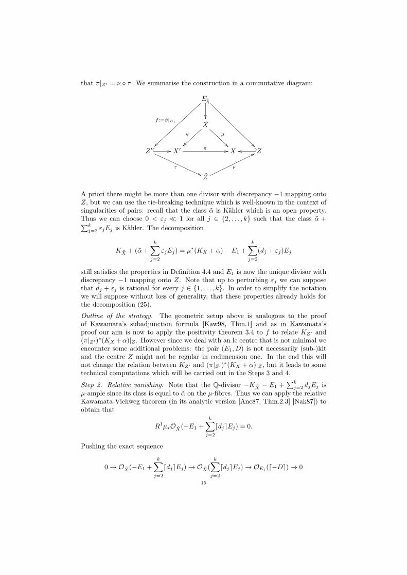
that π|Z′ = ν τ . We summarise the construction in a commutative diagram:

E1

f :=ψ|E1

~~

_

X

ψ

~~

µ

Z ′ //

τ

((

X ′π // X Z? _oo

Z

ν

77

A priori there might be more than one divisor with discrepancy −1 mapping ontoZ, but we can use the tie-breaking technique which is well-known in the context ofsingularities of pairs: recall that the class α is Kähler which is an open property.Thus we can choose 0 < εj 1 for all j ∈ 2, . . . , k such that the class α +∑kj=2 εjEj is Kähler. The decomposition

KX + (α+

k∑j=2

εjEj) = µ∗(KX + α)− E1 +

k∑j=2

(dj + εj)Ej

still satisfies the properties in Definition 4.4 and E1 is now the unique divisor withdiscrepancy −1 mapping onto Z. Note that up to perturbing εj we can supposethat dj + εj is rational for every j ∈ 1, . . . , k. In order to simplify the notationwe will suppose without loss of generality, that these properties already holds forthe decomposition (25).

Outline of the strategy. The geometric setup above is analogous to the proofof Kawamata’s subadjunction formula [Kaw98, Thm.1] and as in Kawamata’sproof our aim is now to apply the positivity theorem 3.4 to f to relate KZ′ and(π|Z′)∗(KX +α)|Z . However since we deal with an lc centre that is not minimal weencounter some additional problems: the pair (E1, D) is not necessarily (sub-)kltand the centre Z might not be regular in codimension one. In the end this willnot change the relation between KZ′ and (π|Z′)∗(KX + α)|Z , but it leads to sometechnical computations which will be carried out in the Steps 3 and 4.

Step 2. Relative vanishing. Note that the Q-divisor −KX − E1 +∑kj=2 djEj is

µ-ample since its class is equal to α on the µ-fibres. Thus we can apply the relativeKawamata-Viehweg theorem (in its analytic version [Anc87, Thm.2.3] [Nak87]) toobtain that

R1µ∗OX(−E1 +

k∑j=2

ddjeEj) = 0.

Pushing the exact sequence

0→ OX(−E1 +

k∑j=2

ddjeEj)→ OX(

k∑j=2

ddjeEj)→ OE1(d−De)→ 0

15

down to X, the vanishing of R1 yields a surjective map

(26) µ∗(OX(

k∑j=2

ddjeEj))→ (µ|E1)∗(OE1(d−De)).

Since all the divisors Ej are µ-exceptional, we see that µ∗(OX(∑kj=2ddjeEj)) is

an ideal sheaf I. Moreover, since dj > −1 for all Ej mapping onto Z the sheafI is isomorphic to the structure sheaf in the generic point of Z . In particular(µ|E1

)∗(OE1(d−De)) has rank one.

Step 3. Application of the positivity result. By the adjunction formula we have

(27) KE1+ α|E1

−k∑j=2

dj(Ej ∩ E1) = f∗(π|Z′)∗(KX + α)|Z .

Since f coincides with µ|E1over the generic point of Z ′, we know by Step 2 that

the direct image sheaf f∗(OE1(d−De)) has rank one. In particular f has connected

fibres.In general the boundary D does not satisfy the conditions a) and b) in Theorem3.4, however we can still obtain some important information by applying Theorem3.4 for a slightly modified boundary: note first that the fibration f is equidimen-sional over the complement of a codimension two set. In particular the directimage sheaf f∗(OE1(d−De)) is reflexive [Har80, Cor.1.7], hence locally free, on thecomplement of a codimension two set. Thus we can consider the first Chern classc1(f∗(OE1

(d−De))) (cf. Definition 2.2). Set

L := (π|Z′)∗(KX + α)|Z −KZ′ ,

then we claim that

(28) (L+ c1(f∗(OE1(d−De)))) · ω′1 · . . . · ω′dimZ−1 ≥ 0

for any collection of nef classes ω′j on Z ′.Proof of the inequality (28). In the complement of a codimension two subset B ⊂ Z ′the fibration f |f−1(Z′\B) is equidimensional, so the direct image sheaf OE1(d−Dve)is reflexive. Since it has rank one we thus can write

f∗(OE1(d−Dve))⊗OZ′\B = OZ′\B(∑

elQl)

where el ∈ Z and Ql ⊂ Z ′ are the prime divisors introduced in the geometric setup.If el > 0 then el is the largest integer such that

(f |f−1(Z′\B))∗(elQl) ⊂ d−Dve.

In particular if Dj maps onto Ql, then dj > −1. If el < 0 there exists a divisor Dj

that maps onto Ql such that dj ≤ −1. Moreover if wj is the coefficient of Dj in thepull-back (f |f−1(Z′\B))

∗Ql, then el is the largest integer such that dj − elwj > −1for every divisor Dj mapping onto Ql. Thus if we set

D := D +∑

elf∗Ql,

then D has normal crossings support (cf. Step 1) and satisfies the condition a)in Theorem 3.4. Moreover if we denote by D = Dh + Dv the decomposition inhorizontal and vertical part, then Dh = Dh and Dv = Dv +

∑elf∗Ql. Since we

16

did not change the horizontal part, the direct image f∗(OE1(d−De)) has rank one.Since

∑elf∗Ql has integral coefficients, the projection formula shows that

(f∗(OE1(d−Dve)))∗∗ ' (f∗(OE1

(d−Dve)))∗∗ ⊗OZ′(−∑

elQl) ' OZ′ .

Thus we satisfy the condition b) in Theorem 3.4. Finally note that

KE1/Z + α|E1 + D = f∗(L+∑

elQl).

So if we set L := L+∑elQl, then

(29) L+ c1(f∗(OE1(d−De))) = L+ c1(f∗(OE1(d−De))).Now we apply Theorem 3.4 and obtain

L · ω′1 · . . . · ω′dimZ′−1 ≥ 0.

Yet by the conditions a) and b) there exists an ideal sheaf I on Z ′ that has cosupportof codimension at least two and f∗(OE1

(d−De)) ' I ⊗OZ′(B) with B an effectivedivisor on Z ′. Thus c1(f∗(OE1

(d−De))) is represented by the effective divisor Band (28) follows from (29).Step 4. Final computation. In view of our definition of the intersection product onZ (cf. Definition 2.7) we are done if we prove that

L · τ∗ω1 · . . . · τ∗ωdimZ−1 ≥ 0

where the ωj are the nef cohomology classes from the statement of Theorem 1.5.We claim that

(30) c1(f∗(OE1(d−De))) = −∆1 + ∆2

where ∆1 is an effective divisor and ∆2 is a divisor such that π|Z′(Supp ∆2) hascodimension at least two in Z. Assuming this claim for the time being let us seehow to conclude: by (28) we have

(31) (L+ c1(f∗(OE1(d−De)))) · τ∗ω1 · . . . · τ∗ωdimZ−1 ≥ 0.

Since the normalisation ν is finite and π|Z′(Supp ∆2) has codimension at least twoin Z, we see that τ(Supp ∆2) has codimension at least two in Z. Thus we have

c1(f∗(OE1(d−De))) · τ∗ω1 · . . . · τ∗ωdimZ−1 = −∆1 · τ∗ω1 · . . . · τ∗ωdimZ−1 ≤ 0.

Hence the statement follows from (31).Proof of the equality (30). Applying as in Step 2 the relative Kawamata-Viehwegvanishing theorem to the morphism ψ we obtain a surjection

ψ∗(OX(

k∑j=2

ddjeEj))→ (ψ|E1)∗(OE1(d−De))

In order to verify (30) note first that some of the divisors Ej might not be ψ-exceptional, so it is not clear if ψ∗(OX(

∑kj=2ddjeEj)) is an ideal sheaf. However if

we restrict the surjection (26) to Z we obtain a surjective map

(32) I ⊗OX OZ → (π|Z′)∗(f∗(OE1(d−De))),where I is the ideal sheaf introduced in Step 2. There exists an analytic set B ⊂ Zof codimension at least two such that

Z ′ \ π−1(B)→ Z \B17

is isomorphic to the normalisation of Z \ B. In particular the restriction of π toZ ′ \ π−1(B) is finite, so the natural map

(π|Z′)∗(π|Z′)∗(f∗(OE1(d−De)))→ f∗(OE1(d−De))

is surjective on Z ′ \ π−1(B). Pulling back is right exact, so composing with thesurjective map (32) we obtain a map from an ideal sheaf to f∗(OE1(d−De)) thatis surjective on Z ′ \ π−1(B). An ideal sheaf is torsion-free, so this map is anisomorphism onto its image in J ⊂ f∗(OE1

(d−De)). In the complement of acodimension two set the sheaf J corresponds to an antieffective divisor −∆′1. Sincethe inclusion J ⊂ f∗(OE1

(d−De)) is an isomorphism on Z ′ \ π−1(B), there existsan effective divisor ∆′2 with support in π−1(B) such that c1(f∗(OE1(d−De))) =−∆′1 + ∆′2. We denote by ∆1 the part of ∆′1 whose support is not mapped intoB (hence maps into the non-normal locus of Z \B) and set ∆2 := ∆′2 + ∆1 −∆′1.Then we have c1(f∗(OE1

(d−De))) = −∆1 + ∆2 and the support of ∆2 maps intoB. Since B has codimension at least two this proves the equality (30).

4.5. Remark. In Step 3 of the proof of Theorem 1.5 above we introduce a “bound-ary” c1(f∗(OM (d−De))) so that we can apply Theorem 3.4. One should note thatthis divisor is fundamentally different from the divisor ∆ appearing in [Kaw98,Thm.1, Thm.2]. In fact for a minimal lc centre Kawamata’s arguments show thatc1(f∗(OM (d−De))) = 0, his boundary divisor ∆ is defined in order to obtain thestronger result that L −∆ is nef. We have to introduce c1(f∗(OM (d−De))) sincewe want to deal with non-minimal centres.

5. Positivity of relative adjoint classes, part 2

Convention : In this section, we use the following convention. Let U be a openset and (fm)m∈N be a sequence of smooth functions on U . We say that

‖fm‖C∞(U) → 0,

if for every open subset V b U and every index α, we have

‖∂αfm‖C0(V ) → 0.

Similarly, in the case (fm)m∈N are smooth formes, we say that ‖fm‖C∞(U) → 0 ifevery component tends to 0 in the above sense.

Before giving the main theorem of this section, we need two preparatory lemmas.The first comes from [Lae02, Part II, Thm 1.3] :

5.1. Lemma.[Lae02, Part II, Thm 1.3] Let X be a compact Kähler manifold andlet α be a closed smooth real 2-form on X. Then we can find a strictly increas-ing sequence of integers (sm)m≥1 and a sequence of hermitian line bundles (notnecessary holomorphic) (Fm, DFm , hFm)m≥1 on X such that

(33) limm→+∞

‖√−1

2πΘhFm

(Fm)− smα‖C∞(X) = 0.

Here DFm is a hermitian connection with respect to the smooth hermitian metrichFm and ΘhFm

(Fm) = DFm DFm .Moreover, let (Wj) be a small Stein cover of X and let eFm,j be a basis of an iso-metric trivialisation of Fm over Wj i.e., ‖eFm,j‖hm = 1. Then we can ask the

18

hermitian connections DFm (under the basis eFm,j) to satisfy the following addi-tional condition: for the (0, 1)-part of DFm on Wj : D′′Fm = ∂ + β0,1

m,j, we have

(34) ‖ 1

smβ0,1m,j‖C∞(Wj) ≤ C‖α‖C∞(X),

where C is a uniform constant independent of j and m.

Proof. Thanks to [Lae02, Part II, Thm 1.3], we can find a strictly increasing integersequence (sm)m≥1 and closed smooth 2-forms (αm)m≥1 on X, such that

limm→+∞

‖αm − smα‖C∞(X) = 0 and αm ∈ H2(X,Z).

Since (Wj) are small Stein open sets, we can find some smooth 1-forms βm,j on Wj

such that

(35)1

2π· dβm,j = αm on Wj and ‖ 1

smβm,j‖C∞(Wj) ≤ C‖α‖C∞(X)

for a constant C independent of m and j.By using the standard construction (cf. for example [Dem, V, Thm 9.5]), theform (βm,j)j induces a hermitian line bundle (Fm, Dm, hFm) on X such that Dm =

d+√−1

2π βm,j with respect to an isometric trivialisation over Wj . Then

‖√−1

2πΘhFm

(Fm)− smα‖C∞(X) = ‖αm − smα‖C∞(X) → 0.

Let β0,1m,j be the (0, 1)-part of βm,j . Then (35) implies (34).

Now we can prove the main theorem of this section.

5.2. Theorem. Let X and Y be two compact Kähler manifolds and let f : X → Ybe a surjective map with connected fibres such that the general fibre F is simplyconnected and

H0(F,Ω2F ) = 0.

Let ω be a Kähler form on X such that c1(KF ) + [ω|F ] is a pseudoeffective class.Then c1(KX/Y ) + [ω] is pseudoeffective.

Proof. Being pseudoeffective is a closed property, so we can assume without loss ofgenerality that c1(KF ) + [ω|F ] is big on F .Step 1: Preparation, Stein Cover.Fix two Kähler metrics ωX , ωY on X and Y respectively. Let h be the smooth her-mitian metric on KX/Y induced by ωX and ωY . Set α :=

√−1

2π Θh(KX/Y ). Thanksto Lemma 5.1, there exist a strictly increasing sequence of integers (sm)m≥1 and asequence of hermitian line bundles (not necessary holomorphic) (Fm, DFm , hFm)m≥1

on X such that

(36) ‖√−1

2πΘhFm

(Fm)− sm(α+ ω)‖C∞(X) → 0.

By our assumption on F we can find a non empty Zariski open subset Y0 of Y suchthat f is smooth over Y0 and Rif∗OX = 0 on Y0 for every i = 1, 2. Let (Ui)i∈I bea Stein cover of Y0. Therefore

(37) H0,2(f−1(Ui),R) = 0 for every i ∈ I.19

Step 2: Construction of the approximate holomorphic line bundles.

Let Θ(0,2)hFm

(Fm) be the (0, 2)-part of ΘhFm(Fm). Thanks to (37) and (36), Θ

(0,2)hFm

(Fm)

is ∂-exact on f−1(Ui) and

(38) ‖Θ(0,2)hFm

(Fm)‖C∞(f−1(Ui)) → 0.

We first construct a sequence of (0, 1)-formes βm on f−1(Ui) such that

(39) Θ(0,2)hFm

(Fm) = ∂βm and ‖βm‖C∞(f−1(Ui)) → 0.

In fact, for every y ∈ Ui, as Xy is compact and H0,2(Xy) = 0, we can find smooth(0, 1)-forms θm on f−1(Ui) such that for every y ∈ Ui

(40) (Θ(0,2)hFm

(Fm)− ∂θm)|Xy = 0 and ‖θm‖C∞(f−1(Ui)) → 0.

Therefore Θ(0,2)hFm

(Fm)− ∂θm =∑j f

?(dtj)∧ γm,j , where (dtj) is a basis of ∧0,1(Ui)

and ‖γm,j‖C∞(f−1(Ui)) → 0. Note that Θ(0,2)hFm

(Fm) − ∂θm is ∂-closed. Then∂γm,j |Xy = 0. As H0,1(Xy) = 0, we can find θ′m,j on f−1(Uj) such that(γm,j − ∂θ′m,j)|Xy = 0 and ‖θ′m,j‖C∞(f−1(Ui)) → 0. As a consequence,

Θ(0,2)hFm

(Fm)− ∂(θm +∑j

f?(dtj) ∧ θ′m,j) = f?γ

for some closed (0, 2)-form γ on Ui and ‖γ‖C∞(Ui) → 0. Together with the factthat Ui is Stein, we can thus find βm satisfies (39).

Thanks to (39), we can find holomorphic line bundles Li,m on f−1(Ui) equippedwith smooth hermitian metrics hi,m such that

(41) ‖√−1

2πΘhFm

(Fm)−√−1

2πΘhi,m(Li,m)‖C∞(f−1(Ui)) → 0.

By construction, we have√−1

2πΘhi,m(Li,m)− sm

√−1

2πΘh(KX/Y ) =

√−1

2πΘhi,m(Li,m)− smα

= (

√−1

2πΘhi,m(Li,m)−

√−1

2πΘhFm

(Fm)) + (

√−1

2πΘhFm

(Fm)− sm(α+ ω)) + smω.

Thanks to the estimates (36) and (41), the first two terms of the right-hand sideof the above equality tends to 0. Therefore we can find a sequence of open setsUi,m b Ui, such that ∪m≥1Ui,m = Ui, Ui,m b Ui,m+1 for every m ∈ N, and

(42)√−1

2πΘhi,m(Li,m)− sm

√−1

2πΘh(KX/Y ) ≥ 0 on f−1(Ui,m).

Step 3: Construction of Bergman kernel type metrics.Let ϕi,m be the sm-Bergman kernel associated to the pair (cf. Remark 3.2)

(43) (Li,m = smKX/Y + (Li,m − smKX/Y ), hi,m)

i.e., ϕi,m(x) := supg∈A

1sm

ln |g|hi,m(x), where

(44) A := g | g ∈ H0(Xf(x), Li,m),

∫Xf(x)

|g|2sm

hi,mωdimXX /f∗ωdimY

Y = 1.

20

Thanks to (42), we can apply Theorem 3.1 to the pair (43) over f−1(Ui,m). Inparticular, we have

(45) (α+ ω) + ddcϕi,m ≥ 0 on f−1(Ui,m).

We recall that ϕi,m is invariant after a normalisation of hi,m, namely, if we replacethe metric hi,m|Xy by c · hi,m|Xy for some constant c > 0, the associated Bergmankernel function ϕi,m|Xy is unchanged cf. Remark 3.2 (3).

Let y ∈ Ui be a generic point. Thanks to the above remark and (41), we can finda constant cy > 0 independent of m, such that cy ≤ hi,m|Xy ≤ c−1

y . Therefore,by mean value inequality, ϕi,m|Xy is uniformly upper bounded. Therefore we candefine

ϕi := limk→+∞

( supm≥k

ϕi,m)?,

where ? is the u.s.c regularization. Thanks to (44), ϕi cannot be identically −∞.Therefore ϕi is a quasi-psh. As ∪m≥1Ui,m = Ui, (45) implies

(46) α+ ω + ddcϕi ≥ 0 on f−1(Ui) in the sense of currents.

Step 4: Final conclusion.We claim thatClaim 1. ϕi = ϕj on f−1(Ui ∩ Uj) for every i, j.Claim 2. For every small Stein open set V in X, we can find a constant CVdepending only on V such that

ϕi(x) ≤ CV for every i and x ∈ V ∩ f−1(Ui).

We postpone the proof of these two claims and finish first the proof of the theorem.Thanks to Claim 1, (ϕi)i∈I defines a global quasi-psh function ϕ on f−1(Y0) and(46) implies that

α+ ω + ddcϕ ≥ 0 on f−1(Y0).

Thanks to Claim 2, we have ϕ ≤ CV on V ∩ f−1(Y0). Therefore ϕ can be extendedas a quasi-psh function on V . Since Claim 2 is true for every small Stein open setV , ϕ can be extended as a quasi-psh function on X and satisfies

α+ ω + ddcϕ ≥ 0 on X.

As a consequence, c1(KX/Y )+[ω] is pseudoeffective and the theorem is proved.

We are left to prove the two claims in the proof of the theorem.

5.3. Lemma. The claim 1 holds, i.e., ϕi = ϕj on f−1(Ui ∩ Uj) for every i, j.

Proof. Let y ∈ Ui ∩ Uj be a generic point. Thanks to (41), we have

(47) limm→+∞

‖√−1

2πΘhi,m(Li,m)|Xy −

√−1

2πΘhj,m(Lj,m)|Xy‖C∞(Xy) = 0.

When m is large enough, (47) implies that

c1(Li,m|Xy ) = c1(Lj,m|Xy ) ∈ H1,1(Xy) ∩H2(Xy,Z).

As Xy is simply connected, Pic0(Xy) = 0. Therefore

(48) Li,m|Xy = Lj,m|Xy for m 1.21

Under the isomorphism of (48), by applying ∂∂-lemma, (47) imply the existence ofconstants cm ∈ R and smooth functions τm ∈ C∞(Xy) such that

hi,m = hj,mecm+τm on Xy and lim

m→+∞‖τm‖C∞(Xy) = 0.

Combining with the construction of ϕi,m and ϕj,m, we know that

‖ϕi,m − ϕj,m‖C0(Xy) ≤ ‖τm‖C0(Xy) → 0.

Therefore

(49) ϕi|Xy = ϕj |XyAs (49) is proved for every generic point y ∈ Ui ∩ Uj , we have

ϕi = ϕj on f−1(Ui ∩ Uj).The lemma is proved.

It remains to prove the claim 2. Note that (Li,m, hi,m) is defined only on f−1(Ui),we can not directly apply Proposition 3.3 to (Li,m, hi,m).The idea of the proof isas follows. Thanks to the construction of Fm and Li,m, by using ∂∂-lemma, wecan prove that, after multiplying by a constant (which depends on f(x) ∈ Y ),the difference between hFm |Xf(x) and hi,m|Xf(x) is uniformly controlled for m 15. Therefore (Fm|Xf(x) , hFm) is not far from (Li,m|Xf(x) , hi,m). Note that, usingagain (36), Fm|V is not far from a holomorphic line bundle over V . CombiningProposition 3.3 with these two facts, we can finally prove the claim 2.

5.4. Lemma. The claim 2 holds, i.e., for every small Stein open set V in X, wecan find a constant CV depending only on V such that

ϕi(x) ≤ CV for every i and x ∈ V ∩ f−1(Ui).

Proof. Step 1: Global approximation.Fix a small Stein cover (Wj)

Nj=1 of X. Without loss of generality, we can assume

that V bW1. Let (Fm, DFm , hFm)m≥1 be the hermitian line bundles (not necessaryholomorphic) constructed in the step 1 of the proof of Theorem 5.2. Let eFm,j bea basis of a isometric trivialisation of Fm over Wj i.e., ‖eFm,j‖hFm = 1. Under thistrivialisation, we suppose that the (0, 1)-part of DFm on Wj is D′′Fm = ∂ + β0,1

m,j ,where β0,1

m,j is a smooth (0, 1)-form on Wj . By Lemma 5.1, we can assume that

(50) ‖ 1

smβ0,1m,j‖C∞(Wj) ≤ C1‖α+ ω‖C∞(X)

for a uniform constant C1 independent of m and j.

Step 2: Local estimation near V .Thanks to (36), we know that Fm is not far from a holomorphic line bundle. Inthis step, we would like to give a more precise description of this on W1.Since W1 is a small Stein open set, thanks to (36), we can find σ0,1

m m≥1 on W1

such that ∂σ0,1m = −Θ

(0,2)hFm

(Fm) and limm→+∞

‖σ0,1m ‖C∞(W1) = 0. Then we have

(51) (D′′F,m + σ0,1m )2 = 0 on W1,

5The bigness of m 1 depends on f(x).22

and

‖√−1

2πΘhFm ,D

′′F,m+σ0,1

m(Fm)− sm(α+ ω)‖C∞(X) → 0,

where ΘhFm ,D′′F,m+σ0,1

m(Fm) is the curvature for the Chern connection on Fm with

respect to complex structure D′′F,m + σ0,1m and the metric hFm .

Note that√−1

2π ΘhFm ,D′′F,m+σ0,1

m(Fm) is a closed (1, 1)-form on W1. By ∂∂-lemma,

we can find smooth functions ψmm≥1 on W1 such that

(i)√−1

2π ΘhFme−ψm ,D′′F,m+σ0,1

m(Fm) = sm(α+ ω) on W1 for every m ∈ N. 6

(ii) limm→+∞

(‖σ0,1m ‖C∞(W1) + ‖ψm‖C∞(W1)) = 0.

Thanks to (51), β0,1m,1 + σ0,1

m is ∂-closed. Applying standard L2-estimate, by re-stricting on some a little bit smaller open subset of W1 (we still denote it by W1

for simplicity), there exists a smooth function ηm on W1 such that

(52) ∂ηm = β0,1m,1 + σ0,1

m on W1

and1

sm‖ηm‖C∞(W1) ≤

C2

sm‖β0,1

m,1 + σ0,1m ‖C∞(W1)

for a constant C2 independent of m. Combining this with (50) and (ii), we get

(53) limm→+∞1

sm‖ηm‖C∞(W1) ≤ C1 · C2.

Moreover, by (52), e−ηm · eFm,1 is a holomorphic basis of (W1, Fm, D′′Fm

+ σ0,1m ).

Step 3: Final conclusion.Let x ∈ V ∩ f−1(Ui) and set y := f(x).Claim. For m large enough, there exists a g ∈ H0(Xy ∩W1, Fm, D

′′Fm

+σ0,1m ). such

that

(54)∫Xy∩W1

|g|2sm

hFmωdimXX /ωdimY

Y ≤ 2

and

(55) ϕi,m(x) ≤ 1

smln |g|hFm (x) + 2.

We postphone the proof of the claim later and first finish the proof of our lemma.

As e−ηm · eFm,1 is a holomorphic basis of (W1, Fm, D′′Fm

+ σ0,1m ), we have

g = f · e−ηm · eFm,1for some holomorphic function f onW1∩Xy. Thanks to (53), we can find a uniformconstant C3 > 0 independent of m such that

(56) C−13 ≤ |e−ηm · eFm,1|

2sm

hFm≤ C3 on W1.

6Here ΘhFme

−ψm ,D′′F,m

+σ0,1m

(Fm) is the curvature for the Chern connection on Fm with re-

spect to complex structure D′′F,m + σ0,1m and the metric hFm · e−ψm .

23

Together with (54), we have∫Xy∩W1

|f |2sm ωdimX

X /ωdimYY ≤ 2C3.

By applying the Ohsawa-Takegoshi extension theorem [BP10, Prop 0.2], we knowthat |f |

2sm is uniformly controled. Together with (56), 1

smln |g|hFm (x) is controled

by a uniform constant C4. Combining this with (55), the lemma is proved.

It remains to prove the claim in Lemma 5.4.

Proof of the claim in Lemma 5.4. By (36) and Pic0(Xy) = 0, when m is largeenough, we can find a smooth (0, 1)-forms τ0,1

m on Xy such that

(57) limm→+∞

‖τ0,1m ‖C∞(Xy) = 0 and (Fm, D

′′Fm + τ0,1

m )|Xy ' Li,m|Xy .

Let ΘhFm ,τ0,1m

(Fm|Xy ) be the curvature calculated for the Chern connection withrespect to hFm and the complex structure D′′Fm + τ0,1

m for the line bundle Fm|Xy .Thanks (36) and (57) imply that

(58) limm→+∞

‖ΘhFm ,τ0,1m

(Fm|Xy )−Θhi,m(Li,m|Xy )‖C∞(Xy) = 0.

By using ∂∂-lemma over Xy, under the holomorphic isomorphism of (57), (58)implies the existence of a constant cm,y and a smooth function ψm on Xy such that

(59) hFm · e−ψm = hi,m · e−cm,y on Xy,

and

(60) limm→+∞

‖ψm‖C∞(Xy) = 0.

Here cm,y is a constant on Xy which depends only on m and y.

By the definition of ϕi,m, there exists a g ∈ H0(Xy, Li,m) such that

(61) ϕi,m(x) =1

smln |g|hi,m(x) and

∫Xy

|g|2sm

hi,mωdimXX /ωdimY

Y = 1.

Using the holomorphic isomorphism (57) and the metric estimations (60) and (59),we can thus find a g ∈ H0(Xy, Fm, D

′′Fm

+ τ0,1m )7 such that

(62)∫Xy

|g|2sm

hFmωdimXX /ωdimY

Y = 1 and ϕi,m(x) ≤ 1

smln |g|hFm (x) + 1

where m is large enough. Here we use Remark 3.2 (3) and the fact that cm,y isconstant on Xy (although it might be very large).

Now we prove the claim. Thanks to (57) and the fact that τ0,1m − σ0,1

m is ∂-exact onthe Stein open set Xy ∩W1, there exists some smooth functions ζm on Xy ∩W1,such that

∂ζm = τ0,1m − σ0,1

m on Xy ∩W1

and

(63) limm→+∞

1

sm‖ζm‖C∞(Xy∩W1) ≤ lim

m→+∞

Cysm‖τ0,1m − σ0,1

m ‖C∞(Xy∩W1) = 0.

7It means that g is a holomorphic section of Fm on Xy with respect to the complex structureD′′Fm + τ0,1m .

24

for a constant Cy independent of m, but depending on y.

Set g := eζm · g. Then g ∈ H0(Xy ∩W1, Fm, D′′Fm

+σ0,1m ). Thanks to (63) and (62),

when m is large enough, we have

(64)∫Xy∩W1

|g|2sm

hFmωdimXX /ωdimY

Y ≤ 2

and

(65) ϕi,m(x) ≤ 1

smln |g|hFm (x) + 2.

The claim is proved.

6. Proof of the main theorem

We start with an easy, but important lemma relating null locus and lc centres.

6.1. Lemma. Let X be a compact Kähler manifold, and let α be a nef and bigclass such that the null locus Null(α) has no divisorial components. Let Z ⊂ Xbe an irreducible component of Null(α). Then there exists a positive real number csuch that Z is a maximal lc centre for (X, cα).

Remark. The coefficient c depends on the choice of Z, so in general the otherirreducible components of Null(α) will not be lc centres for (X, cα).

Proof. By a theorem of Collins of Tosatti [CT15, Thm.1.1] the non-Kähler locusEnK(α) coincides with the null-locus of Null(α). Moreover by [Bou04, Thm.3.17]there exists a Kähler current T with analytic singularities in the class α such thatthe Lelong set coincides with EnK(α). Since the non-Kähler locus has no divisorialcomponents the class α is a modified Kähler class [Bou04, Defn.2.2]. By [Bou04,Prop.2.3] the class α has a log-resolution µ : X → X such that µ∗α = α. In factthe proof proceeds by desingularising a Kähler current with analytic singularitiesin the class α, so, using the current T defined above, we see that the µ-exceptionallocus maps exactly onto Null(α). Up to blowing up further the exceptional locus isa SNC divisor. By Remark 4.3 we have

µ∗α = α+

k∑j=1

rjDj .

with rj > 0 for all j ∈ 1, . . . , k. Since α is nef and big, the class α + mµ∗α isKähler for all m > 0. Thus up to replacing the decomposition above by

µ∗α =α+mµ∗α

m+ 1+

k∑j=1

rjm+ 1

Dj

for m 0 we can suppose that rj < 1 for all j ∈ 1, . . . , k. Since X is smoothwe have KX = µ∗KX +

∑kj=1 ajEj with aj a positive integer. Since rj < 1 we

have aj − rj > −1 for all Ej mapping onto Z. Thus we can choose a c ∈ R+ suchthat aj − crj ≥ −1 for all Ej mapping onto Z and equality holds for at least onedivisor.

As a first step toward Theorem 1.3 we can now prove the following:25

6.2. Theorem. Let X be a compact Kähler manifold of dimension n. Supposethat Conjecture 1.2 holds for all manifolds of dimension at most n − 1. Supposethat KX is pseudoeffective but not nef, and let ω be a Kähler class on X such thatα := KX + ω is nef and big but not Kähler.Let Z ⊂ X be an irreducible component of maximal dimension of the null-locusNull(α), and let π : Z ′ → Z be the composition of the normalisation and a resolutionof singularities. Let k be the numerical dimension of π∗α|Z (cf. Definition 2.5).Then we have

KZ′ · π∗α|kZ · π∗ω|dimZ−k−1Z < 0.

In particular Z ′ is uniruled.

Proof of Theorem 6.2. Since α = KX + ω and π∗α|k+1Z = 0 we have

π∗KX |Z · π∗α|kZ = −π∗ω|Z · π∗α|kZ .By hypothesis k < dimZ so dimZ−k−1 is non-negative. Since π∗α|kZ is a non-zeronef class and ω is Kähler this implies by Remark 2.6 that

(66) π∗KX |Z · π∗α|kZ · π∗ω|dimZ−k−1Z = −π∗ω|dimZ−k

Z · π∗α|kZ < 0.

Our goal will be to prove that

KZ′ · π∗α|kZ · π∗ω|dimZ−k−1Z < 0.

This inequality implies the statement: since KZ′ is not pseudoeffective and Conjec-ture 1.2 holds in dimension at most n− 1 ≥ dimZ ′ we obtain that Z ′ is uniruled.We will make a case distinction:Step 1. The null-locus of α contains an irreducible divisor. Since Z has maximaldimension, it is a divisor. Since KX is pseudoeffective we can consider the divisorialZariski decomposition [Bou04, Defn.3.7]

c1(KX) =∑

eiZi + P (KX),

where ei ≥ 0, the Zi ⊂ X are prime divisors and P (KX) is a modified nef class[Bou04, Defn.2.2]. Arguing as in [HP16, Lemma 4.1] we see that the inequality (66)implies (up to renumbering) that Z1 = Z and

(67) π∗(c1(OZ(Z))) · π∗α|kZ · π∗ω|n−k−2Z < 0.

Thus the normal bundle NZ/X ' OZ(Z) is negative with respect to these nefclasses. Moreover there exist effective Q-divisors on D1 and D2 on Z ′ such that

KZ′ = π∗(KX + Z) +D1 −D2

and π(D1) has codimension at least two in Z (cf. [Rei94, Prop.2.3]). Thus we have

KZ′ · π∗α|kZ · π∗ω|n−k−2Z ≤ π∗(KX + Z) · π∗α|kZ · π∗ω|n−k−2

Z .

Combining (66) and (67) we obtain that the right hand side is negative.Step 2. The null-locus of α has no divisorial components. In this case we know byLemma 6.1 that there exists a c > 0 such that Z is a maximal lc centre for (X, cα).The classes π∗α|Z and π∗ω|Z are nef, so by Theorem 1.5 we have

KZ′ · π∗α|kZ · π∗ω|dimZ−k−1Z ≤ π∗(KX + cα)|Z · π∗α|kZ · π∗ω|dimZ−k−1

Z .

Since k is the numerical dimension of π∗α|Z we have c π∗α|k+1Z ·π∗ω|dimZ−k−1

Z = 0.Thus (66) yields the claim.

26

6.3. Remark. We used the hypothesis that Z has maximal dimension only inStep 1, so our proof actually yields a more precise statement: Null(α) contains auniruled divisor or all the components of Null(α) are uniruled.

We come now to the technical problem mentioned in the introduction:

6.4. Problem. Let X be a compact Kähler manifold, and let α ∈ N1(X) be anef cohomology class. Does there exist a real number b > 0 such that for every(rational) curve C ⊂ X we have either α · C = 0 or α · C ≥ b ?6.5. Remark. If α is the class of a nef Q-divisor, the answer is obviously yes: somepositive multiple mα is integral, so we can choose b := 1

m . If α is a Kähler class theanswer is also yes: by Bishop’s theorem there are only finitely many deformationfamilies of curves C such that α · C ≤ 1, so α · C takes only finitely many valuesin ]0, 1[. However, even for the class of an R-divisor on a projective manifold X itseems possible that the values α · C accumulate at 0 [Laz04, Rem.1.3.12]. In theproof of Theorem 1.3 we will use that α is an adjoint class to obtain the existenceof the lower bound b.

The problem 6.4 is invariant under certain birational morphisms:

6.6. Lemma. Let π : X → X ′ be a holomorphic map between normal projectivevarieties X and X ′. Let α′ be a nef R-divisor class on X ′ and set α := π∗α′.a) Suppose that there exists a real number b > 0 such that for every (rational) curveC ′ ⊂ X ′ we have α′ ·C ′ = 0 or α′ ·C ′ ≥ b. Then for every (rational) curve C ⊂ Xwe have α · C = 0 or α · C ≥ b.b) Suppose that there exists a real number b > 0 such that for every (rational) curveC ⊂ X we have α · C = 0 or α · C ≥ b. Suppose also that X has klt singularitiesand π is the contraction of a KX-negative extremal ray. Then for every (rational)curve C ′ ⊂ X ′ we have α′ · C ′ = 0 or α′ · C ′ ≥ b.

Proof. Proof of a) Let C ⊂ X be a (rational) curve such that α ·C 6= 0. the imageC ′ := π(C) ⊂ X ′ is a (rational) curve and the induced map C → C ′ has degreed ≥ 1. Thus the projection formula yields

α · C = π∗α′ · C = α′ · π∗(C) = dα′ · C ′ ≥ db ≥ b.

Proof of b) Let C ′ ⊂ X ′ be an arbitrary (rational) curve such that α′ · C ′ 6= 0. By[HM07, Cor.1.7(2)] the natural map π−1(C ′)→ C ′ has a section, so there exists a(rational) curve C ⊂ X such that the map π|C : C → C ′ has degree one. Thus theprojection formula yields

α′ · C ′ = α′ · π∗(C) = π∗α · C ≥ b.

6.7. Remark. It is easy to see that statement a) also holds when X and X ′ arecompact Kähler manifolds and α′ is a nef cohomology class on X ′.

6.8. Corollary. Let X be a normal projective Q-factorial variety with klt singu-larities, and let α be a nef R-divisor class on X. Suppose that there exists a realnumber b > 0 such that for every (rational) curve C ⊂ X we have α · C = 0 orα · C ≥ b. Let µ : X 99K X ′ be the divisorial contraction or flip of a KX-negativeextremal ray Γ such that α · Γ = 0. Set α′ := µ∗(α). Then α′ is a nef R-divisorclass on X ′ and for every (rational) curve C ⊂ X we have α · C = 0 or α · C ≥ b.

27

Proof. If µ is divisorial the condition α · Γ = 0 implies that α = µ∗α′ [KM98,Cor.3.17]. Thus Lemma 6.6, b) applies. If µ is a flip, let f : X → Y be thecontraction of the extremal ray and f ′ : X ′ → Y the flipping map. Since α · Γ = 0there exists an R-divisor class αY on Y such that α = f∗αY [KM98, Cor.3.17].Moreover we have α′ = (f ′)∗αY since they coincide in the complement of theflipped locus. Thus we conclude by applying Lemma 6.6,b) to f and Lemma 6.6,a)to f ′.

6.9. Proposition. Let F be a projective manifold, and let α be a nef R-divisorclass on F . Suppose that there exists a real number b > 0 such that for everyrational curve C ⊂ F such that α · C 6= 0 we have

(68) α · C > b.

Then one of the following holds

• F is dominated by rational curves C ⊂ F such that α · C = 0; or• the class KF + 2 dimF

b α is pseudoeffective.

Proof. Note that, up to replacing α by 2 dimFb α, we can suppose that

(69) α · C > 2 dimF

for every rational curve C ⊂ F that is not α-trivial. Suppose that KF + α is notpseudoeffective, then our goal is to show that F is covered by α-trivial rationalcurves. Since KF + α is not pseudoeffective, there exists an ample R-divisor Hsuch that KF +α+H is not pseudoeffective. Since H and α+H are ample we canchoose effective R-divisors ∆H ∼R H and ∆ ∼R α+H such that the pairs (F,∆H)and (F,∆) are klt. By [BCHM10, Cor.1.3.3] we can run a KF + ∆-MMP

(F,∆) =: (F0,∆0)µ099K (F1,∆1)

µ199K . . .

µk99K (Fk,∆k),

that is for every i ∈ 0, . . . , k − 1 the map µi : Fi 99K Fi+1 is either a divisorialMori contraction of a KFi + ∆i-negative extremal ray Γi in NE(Xi) or the flip ofa small contraction of such an extremal ray. Note that for every i ∈ 0, . . . , k thevariety Fi is normal Q-factorial and the pair (Fi,∆i) is klt. Moreover Fk admitsa Mori contraction of fibre type ψ : Fk → Y contracting an extremal ray Γk suchthat (KFk + ∆k) · Γk < 0.Set ∆H,0 := ∆H , α0 := α and for all i ∈ 0, . . . , k − 1 we define inductively

∆H,i+1 := (µi)∗(∆H,i), αi+1 := (µi)∗(αi).

Note that for all i ∈ 0, . . . , k we have

(70) KFi + ∆i ≡ KFi + ∆H,i + αi.

We claim that for all i ∈ 0, . . . , k the R-divisor class αi is nef and αi · Γi = 0.Moreover the pairs (Xi,∆H,i) are klt. Assuming this for the time being, let us seehow to conclude: since ψ : Fk → Y is a Mori fibre space and the extremal ray Γkis αk-trivial, we see that Fk is dominated by αk-trivial rational curves (Ct)t∈T . Ageneral member of this family of rational curves is not contained in the exceptionallocus of F0 99K Fk, so the strict transforms define a dominant family of rationalcurves (C ′t)t∈T of F0. Since all the birational contractions in the MMP F0 99K Fkare α•-trivial, we easily see (cf. the proof of Corollary 6.8) that

α · C ′t = αk · Ct = 0.28

Proof of the claim. Since α0 is nef, we have

0 > (KF0 + ∆0) · Γ0 = (KF0 + ∆H,0 + α0) · Γ0 ≥ (KF0 + ∆H,0) · Γ0.

Thus the extremal ray Γ0 is KF0 + ∆H,0-negative, in particular the pair (F1,∆1)is klt [KM98, Cor.3.42, 3.43]. Moreover there exists by [Kaw91, Thm.1] a rationalcurve [C0] ∈ Γ0 such that (KF0

+ ∆H,0) · C0 ≥ −2 dimF . Thus if α0 · C0 6= 0, theinequality (69) implies that

(KF0+ ∆0) · C0 = (KF0

+ ∆H,0) · C0 + α0 · C0 > 0.

In particular the extremal ray Γ0 is not KF0+ ∆0-negative, a contradiction to our

assumption. Thus we have α0 ·C0 = 0. By Corollary 6.8 this implies that α1 is nefand satisfies the inequality (69). The claim now follows by induction on i.

6.10. Remark. For the proof of Theorem 1.3 we will use the MRC fibration of auniruled manifold. Since the original papers [KMM92, Cam92] are formulated forprojective manifolds, let us recall that for a compact Kähler manifold M that isuniruled the MRC fibration is defined as an almost holomorphic map f : M 99K Nsuch that the general fibre F is rationally connected and the dimension of F ismaximal among all the fibrations of this type. The existence of the MRC fibrationfollows, as in the projective case, from the existence of a quotient map for coveringfamilies [Cam04]. The base N is not uniruled : arguing by contradiction we considera dominating family (Ct)t∈T of rational curves on N . LetMt be a desingularisationof f−1(Ct) for a general Ct, then Mt is a compact Kähler manifold with a fibrationonto a curve Mt → Ct such that the general fibre is rationally connected. Inparticular H0(Mt,Ω

2Mt

) = 0 so Mt is projective by Kodaira’s criterion. Thus wecan apply the Graber-Harris-Starr theorem [GHS03] to see that Mt is rationallyconnected, a contradiction.

Proof of Theorem 1.3. Let ω be a Kähler class such that α := KX + ω is nef andbig, but not Kähler. By Theorem 6.2 there exists a subvariety Z ⊂ X containedin the null-locus Null(α) that is uniruled. More precisely let π : Z ′ → Z be adesingularisation, and denote by k the numerical dimension of α′ := π∗α|Z . Thenwe know by Theorem 6.2 that

KZ′ · α′k · π∗ω|dimZ−k−1Z < 0.

Since α′k+1 = 0 this actually implies that

(71) (KZ′ + λα′) · α′k · π∗ω|dimZ−k−1Z < 0 ∀ λ > 0.

Our goal is to prove that this implies that Z contains a KX -negative rationalcurve. Arguing by contradiction we suppose that KX · C ≥ 0 for every rationalcurve C ⊂ Z. Since ω is a Kähler class this implies by Remark 6.5 that there existsa b > 0 such that for every rational curve C ⊂ Z we have

(72) α · C = (KX + ω) · C ≥ ω · C ≥ b.By Lemma 6.6a) and Remark 6.7 this implies that for every rational curve C ′ ⊂ Z ′we have α′ · C ′ = 0 or α′ · C ′ ≥ b.Since Z ′ is uniruled we can consider the MRC-fibration f : Z ′ 99K Y (cf. Remark6.10). The general fibre F is rationally connected, in particular we can consider α′|Fas a nef R-divisor class. Moreover the inequality above shows that α′|F satisfiesthe condition (68) in Proposition 6.9. If F is dominated by α′|F -trivial rational

29

curves, then Z ′ is dominated by α′-trivial rational curves. A general member ofthis dominating family is not contracted by π, so Z is dominated by α-trivialrational curves. This possibility is excluded by (72), so Proposition 6.9 shows thatthere exists a λ > 0 such that KF + λα′|F is pseudoeffective.We will now prove that KZ′ +λα is pseudoeffective, which clearly contradicts (71).If ν : Z ′′ → Z is a resolution of the indeterminacies of f such that KZ′′ + ν∗(λα) ispseudoeffective, then KZ′ + λα = (ν)∗(KZ′′ + ν∗(λα)) is pseudoeffective. Thus wecan assume without loss of generality that the MRC-fibration f is a holomorphicmap. Let ω′ be a Kähler class on Z ′, then for every ε > 0 the class λα′ + εω isKähler and KF + (λα+ εω)|F is pseudoeffective. Thus we can apply Theorem 5.2to f : Z ′ → Y to see that

KZ′/Y + λα+ εω

is pseudoeffective. Note now that Y has dimension at most dimX − 2 is notuniruled (Remark 6.10) Since we assume that Conjecture 1.2 holds in dimension upto dimX−1, we obtain that KY is pseudoeffective. Thus we see that KZ′+λα+εωis pseudoeffective for all ε > 0. The statement follows by taking the limit ε→ 0.

References

[Anc87] Vincenzo Ancona. Vanishing and nonvanishing theorems for numerically effective linebundles on complex spaces. Ann. Mat. Pura Appl. (4), 149:153–164, 1987.

[Ara10] Carolina Araujo. The cone of pseudo-effective divisors of log varieties after Batyrev.Math. Z., 264(1):179–193, 2010.

[BCHM10] Caucher Birkar, Paolo Cascini, Christopher D. Hacon, and James McKernan. Ex-istence of minimal models for varieties of log general type. J. Amer. Math. Soc.,23(2):405–468, 2010.

[BDPP13] Sébastien Boucksom, Jean-Pierre Demailly, Mihai Păun, and Thomas Peternell. Thepseudo-effective cone of a compact Kähler manifold and varieties of negative Kodairadimension. Journal of Algebraic Geometry, 22:201–248, 2013.

[BHN15] Mauro C. Beltrametti, Andreas Höring, and Carla Novelli. Fano varieties with smallnon-klt locus. Int. Math. Res. Not. IMRN, (11):3094–3120, 2015.

[Bou04] Sébastien Boucksom. Divisorial Zariski decompositions on compact complex manifolds.Ann. Sci. École Norm. Sup. (4), 37(1):45–76, 2004.

[BP08] Bo Berndtsson and Mihai Păun. Bergman kernels and the pseudoeffectivity of relativecanonical bundles. Duke Math. J., 145(2):341–378, 2008.

[BP10] Bo Berndtsson and Mihai Păun. Bergman kernels and subadjunction. ArXiv e-prints,February 2010.

[Bru06] Marco Brunella. A positivity property for foliations on compact Kähler manifolds.Internat. J. Math., 17(1):35–43, 2006.

[Cam92] Frédéric Campana. Connexité rationnelle des variétés de Fano. Ann. Sci. École Norm.Sup. (4), 25(5):539–545, 1992.

[Cam04] Frédéric Campana. Orbifolds, special varieties and classification theory: an appendix.Ann. Inst. Fourier (Grenoble), 54(3):631–665, 2004.

[Cao14] Junyan Cao. Ohsawa-Takegoshi extension theorem for compact Kähler manifolds andapplications. ArXiv e-prints, April 2014.

[CP90] Frédéric Campana and Thomas Peternell. Algebraicity of the ample cone of projectivevarieties. J. Reine Angew. Math., 407:160–166, 1990.

[CT15] Tristan C. Collins and Valentino Tosatti. Kähler currents and null loci. Invent.Math.,202(3):1167–1198, 2015.

[Dem] Jean-Pierre Demailly. Complex analytic and differential geometry. http://www-fourier.ujf-grenoble.fr/∼demailly/documents.html.

[Dem12] Jean-Pierre Demailly. Analytic methods in algebraic geometry, volume 1 of Surveys ofModern Mathematics. International Press, Somerville, MA; Higher Education Press,Beijing, 2012.

30

[DP04] Jean-Pierre Demailly and Mihai Păun. Numerical characterization of the Kähler coneof a compact Kähler manifold. Ann. of Math. (2), 159(3):1247–1274, 2004.

[FG12] Osamu Fujino and Yoshinori Gongyo. On canonical bundle formulas and subadjunc-tions. Michigan Math. J., 61(2):255–264, 2012.

[FM00] Osamu Fujino and Shigefumi Mori. A canonical bundle formula. J. Differential Geom.,56(1):167–188, 2000.

[GHS03] Tom Graber, Joe Harris, and Jason Starr. Families of rationally connected varieties.J. Amer. Math. Soc., 16(1):57–67 (electronic), 2003.

[Gue16] H. Guenancia. Families of conic K\“ahler-Einstein metrics. ArXiv e-prints, May 2016.[GZ15] Qi’an Guan and Xiangyu Zhou. A solution of an l2 extension problem with an optimal

estimate and applications. Annals of Mathematics, 181:1139–1208, 2015.[Har77] Robin Hartshorne. Algebraic geometry. Springer-Verlag, New York, 1977. Graduate

Texts in Mathematics, No. 52.[Har80] Robin Hartshorne. Stable reflexive sheaves. Math. Ann., 254(2):121–176, 1980.[HM05] Christopher Hacon and James McKernan. On the existence of flips. arXiv preprint,

0507597, 2005.[HM07] Christopher D. Hacon and James Mckernan. On Shokurov’s rational connectedness

conjecture. Duke Math. J., 138(1):119–136, 2007.[HP16] Andreas Höring and Thomas Peternell. Minimal models for Kähler threefolds. Invent.

Math., 203(1):217–264, 2016.[Kaw91] Yujiro Kawamata. On the length of an extremal rational curve. Invent. Math.,

105(3):609–611, 1991.[Kaw98] Yujiro Kawamata. Subadjunction of log canonical divisors. II. Amer. J. Math.,

120(5):893–899, 1998.[KK83] Ludger Kaup and Burchard Kaup. Holomorphic functions of several variables, vol-

ume 3 of de Gruyter Studies in Mathematics. Walter de Gruyter & Co., Berlin, 1983.[KM98] János Kollár and Shigefumi Mori. Birational geometry of algebraic varieties, volume

134 of Cambridge Tracts in Mathematics. Cambridge University Press, Cambridge,1998. With the collaboration of C. H. Clemens and A. Corti.

[KMM92] Janos Kollár, Yoichi Miyaoka, and Shigefumi Mori. Rational connectedness and bound-edness of Fano manifolds. J. Diff. Geom. 36, pages 765–769, 1992.

[Lae02] Laurent Laeng. Estimations spectrales asymptotiques en géométrie hermitienne.Theses, Université Joseph-Fourier - Grenoble I, October 2002. https://tel.archives-ouvertes.fr/tel-00002098.

[Laz04] Robert Lazarsfeld. Positivity in algebraic geometry. I, volume 48 of Ergebnisse derMathematik und ihrer Grenzgebiete. Springer-Verlag, Berlin, 2004. Classical setting:line bundles and linear series.

[MM86] Yoichi Miyaoka and Shigefumi Mori. A numerical criterion for uniruledness. Ann. ofMath. (2), 124(1):65–69, 1986.

[Mor79] Shigefumi Mori. Projective manifolds with ample tangent bundles. Ann. of Math. (2),110(3):593–606, 1979.

[Mor82] Shigefumi Mori. Threefolds whose canonical bundles are not numerically effective.Ann. of Math. (2), 116(1):133–176, 1982.

[Nak87] Noboru Nakayama. The lower semicontinuity of the plurigenera of complex varieties.In Algebraic geometry, Sendai, 1985, volume 10 of Adv. Stud. Pure Math., pages551–590. North-Holland, Amsterdam, 1987.

[Pău12a] Mihai Păun. Relative adjoint transcendental classes and Albanese maps of compactKähler manifolds with nef Ricci curvature. arXiv preprint, 1209.2195, 2012.

[Pău12b] Mihai Păun. Relative critical exponents, non-vanishing and metrics with minimal sin-gularities. Invent. Math., 187(1):195–258, 2012.

[Rei94] Miles Reid. Nonnormal del Pezzo surfaces. Publ. Res. Inst. Math. Sci., 30(5):695–727,1994.

[Sch12] Georg Schumacher. Positivity of relative canonical bundles and applications. Invent.Math., 190(1):1–56, 2012.

[Tak06] Shigeharu Takayama. Pluricanonical systems on algebraic varieties of general type.Invent. Math., 165(3):551–587, 2006.

[Tak08] Shigeharu Takayama. On the uniruledness of stable base loci. J. Differential Geom.,78(3):521–541, 2008.

31

[Yi14] Li Yi. An Ohsawa-Takegoshi theorem on compact Kähler manifolds. Sci. China Math.,57(1):9–30, 2014.

Junyan Cao, Institut de Mathématiques de Jussieu, Université Pierre et Marie Curie,Case 247, 4 Place Jussieu, 75252 Paris Cedex, FranceE-mail address: Junyan.CAO@imj-prg.fr

Andreas Höring, Laboratoire de Mathématiques J.A. Dieudonné, UMR 7351 CNRS,Université de Nice Sophia-Antipolis, 06108 Nice Cedex 02, FranceE-mail address: hoering@unice.fr

32