Embed Size (px)
Citation preview

Home Production and the Optimal Rate ofUnemployment Insurance ∗
Yavuz Arslan†
Bank for International Settlements
Bulent Guler‡
Indiana University
Temel Taskin§
World Bank
May, 2015
Abstract
In this paper, we incorporate home production into a quantitative model ofunemployment and show that realistic levels of home production have a signifi-cant impact on the optimal unemployment insurance rate. Motivated by recentlydocumented empirical facts, we augment an incomplete markets model of unem-ployment with a home production technology, which allows unemployed workersto use their extra non-market time as partial insurance against the drop in incomedue to unemployment. Depending on the definition of home production, we findthat the optimal replacement rate is between 47% and 63% of wages, which is sig-nificantly lower than the no home production model’s optimal replacement rate of74%. The calculated range of the optimal rate is also close to the estimated ratesin practice. The fact that home production makes a significant difference in theoptimal unemployment insurance rate is robust to a variety of parameterizations.
∗An older version of this paper was a part of Temel Taskin’s Ph.D. thesis at the University ofRochester and circulated with title “Unemployment Insurance and Home Production”. The authorswould like to thank Mark Aguiar, Arpad Abraham, Mark Bils, Yongsung Chang, Gregorio Caetano, andthe seminar and conference participants at the University of Rochester, European University Institute,Central European University, Izmir Economy University, Middle East Technical University, Central Bankof Turkey, Bilkent University, SED Meeting in Montreal, Midwest Macro Meeting at Michigan StateUniversity, Canadian Economic Association Meeting in Quebec City, Max Weber-Lustrum Conferencein Florence, the ASSET Conference in Evora, Swiss Society of Economics and Statistics Meeting inZurich for helpful discussions. All errors are ours and comments are very welcome. The views expressedhere are those of the authors and do not reflect those of the Central Bank of Turkey.
†Email: [email protected]‡Email: [email protected] URL: http://mypage.iu.edu/˜bguler§Corresponding author. Address: Ugur Mumcu Cad. No:88 Gaziosmanpasa Ankara TURKEY.
Email: [email protected] URL: http://www.temeltaskin.com
1

J.E.L. Classification: D13, E21, J65.Keywords: Unemployment insurance, home production, incomplete markets, self-insurance.
1 Introduction
In this paper, we study the optimal rate of unemployment insurance in an economy
where individuals do home production as well as market production. If there were
complete private insurance against unemployment shocks, then government-provided
unemployment insurance would be unnecessary. Therefore, it is important to account
for the amount of self-insurance of unemployed workers when designing unemployment
insurance programs. We consider home production as a self-insurance mechanism and
study the role of home production in determining the optimal unemployment insurance
rate. The results suggest that the optimal replacement rate in the presence of home
production lies in between 47% and 63% of wages, which is significantly lower than that
of the no-home production case of 74%. The computed range of optimal rate is also close
to the estimated rates in practice for the United States.
Before we pursue a quantitative analysis of optimal replacement rate (benefits/wages)
we provide empirical evidence on the relationship between employment status and time
spent for home production using the American Time Use Survey (ATUS). We find that
unemployed do about 12 hours/week more home production than that of employed.1 We
interpret this difference as a self-insurance mechanism against the loss of earnings during
unemployment spell and account for this fact when we compute the optimal replacement
rate.
To formalize the idea of self-insurance through home production, we augment an in-
complete markets model of unemployment with a home production technology, which al-
1Burda and Hamermesh (2010) provide similar evidence.
2

lows unemployed workers to use their extra non-market time as partial insurance against
the drop in income due to unemployment. The model features a heterogeneous agent
framework due to idiosyncratic employment shocks. Government provides unemploy-
ment insurance as a constant fraction of lost earnings during the unemployment spell,
which is the current design of policy implemented in the United States. It is financed
through proportional income taxation. Along with government-provided unemployment
insurance, individuals can partially self-insure by increasing home production during
unemployment spells and/or accumulating savings.
The role of home production in determining the optimal rate of unemployment in-
surance is quantified by solving the model twice: once with home production and once
without home production. By introducing home production into the model, we dif-
ferentiate consumption from expenditure, which is not an accurate measure of actual
consumption.2 Due to the nature of the unemployment shocks, the budget and time
constraints of individuals change during unemployment spells. They have looser time
constraints and tighter budget constraints, and their optimal behavior adjusts accord-
ingly. In equilibrium, individuals do more home production during unemployment spells,
which provides smoother consumption in comparison with the case in which there is no
home production. Eventually, the optimal rate of unemployment insurance turns out to
be significantly smaller due to the additional self-insurance through home production.
This result is robust to a variety of parameterizations.
The paper contributes to the quantitative unemployment insurance literature by com-
puting the optimal rate of unemployment insurance in an economy where individuals do
home production as well as market production. In general, incomplete asset market mod-
els - including the quantitative models of unemployment insurance - ignore the partial
insurance role of home production and how it varies with employment status.3 However,
2See Aguiar and Hurst (2005, 2007).3For examples of quantitative models on unemployment insurance see: Hansen and Imrohoroglu
3

the recent empirical literature provides evidence that home production is quantitatively
important in time-use surveys.4 In particular, the unemployed allocate their non-market
time differently, and this is important for policy analysis.5 Therefore, our paper closes
the gap between the home production literature and unemployment insurance literature.
The rest of the paper is organized as follows. Section 2 summarizes the related lit-
erature. Section 3 presents some interesting facts about employment status and home
production. Section 4 describes the model in which we analyze the optimal unemploy-
ment insurance. Section 5 presents the quantitative results. Finally, Section 6 concludes.
2 Related Literature
Our paper stands between two bodies of research: first one is the quantitative unem-
ployment insurance literature, and the other is the recent empirical literature on home
production. Many papers, including Hansen and Imrohoroglu (1992), Davidson and
Woodbury (1997), Acemoglu and Shimer (2000), and Chetty (2008), look for the opti-
mal rate of unemployment insurance conditioning on a certain type of policy as we do
in this paper. Our paper differs from those studies in the sense that we consider home
production as well as market production in the model economy.
There is a large literature on the optimal profile of unemployment insurance pay-
ments over the unemployment spell. The results vary. Some of the studies (Shavell
and Weiss 1979, Hopenhayn and Nicolini 1997, Wang and Williamson 2002, Alvarez and
Sanchez 2010) claim that the optimal profile of payments should be decreasing over the
unemployment spell. Other papers (Kocherlakota 2004, Hagedorn et al. 2005, Shimer
and Werning 2008) support flat or increasing payments over the unemployment spell. In
(1992), Hopenhayn and Nicolini (1997), Acemoglu and Shimer (2000). See Heathcote et al. (2009) fora survey on the partial insurance mechanisms in incomplete markets.
4See Aguiar and Hurst (2007).5See Burda and Hamermesh (2010), and Guler and Taskin (2013).
4

this paper, we abstract from the problem of optimal design. Instead, we focus on the
current design in practice in the United States and look for the optimal rate of insurance
conditional on the design in practice.
On the other hand, because of the recent availability of time-use surveys, the number
of studies emphasizing the role of home production has increased substantially. In par-
ticular, using time-use data from some developed countries, including the U.S., Burda
and Hamermesh (2010) document that time spent on home production increases signifi-
cantly due to unemployment. Guler and Taskin (2013) provide empirical evidence on the
negative correlation between time spent for home production and level of unemployment
benefits using American Time Use Survey and state level unemployment benefits data.
Moreover, Aguiar and Hurst (2007) estimate parameters of a home production function
for the U.S. by using two micro data sets.
Moreover, the home production approach has been employed to explain various puz-
zles in macroeconomics. Aguiar and Hurst (2005) explain the retirement puzzle using a
home production approach, where home production has a consumption-smoothing role.
Chang and Hornstein (2007) employ home production in a business cycle model to better
understand aggregate fluctuations in labor supply and the small correlation between em-
ployment and wages. Benhabib et al. (1991), Greenwood and Hercowitz (1991), Canova
and Ubide (1998), and Chang (2000) are other examples. In contrast, motivated by
recent empirical facts, we employ home production as a self-insurance mechanism in a
quantitative unemployment insurance model.
5

3 Data
In this section, we provide complementary results to the recent empirical literature on
home production.6 In particular, we document the relationship between employment
status and home production using the American Time Use Survey (ATUS). It is a re-
peated cross-sectional data set which is a supplement to the Current Population Survey
(CPS). It has been conducted since 2003, and it is nationally representative. We use
2003-2008 samples, which were obtained from the Bureau of Labor Statistics web page.7
The survey collects information through time-use diaries from individuals. It measures
time spent on a rich set of activities, including personal care, household activities, work-
related activities, education, socializing, leisure, traveling and volunteer activities.8 The
unit of time is minutes per day, and we convert it to hours per week by multiplying by
7/60. Also, the survey provides detailed information about the employment status and
demographic characteristics of individuals.
The type of activities considered in the benchmark definition of home production are
time spent on housework, home and vehicle maintenance, consumer purchases, gardening,
pet care, child care and adult care, and travel related to these activities.9 A narrower
definition of home production excludes the time spent for caring for household members
(child care and adult care).
Table 1 presents the average time spent for home production with respect to demo-
graphic features of individuals. As shown in the table, there is a significant difference
between home production of unemployed and employed. We test whether this is still true
when we account for observable differences between these two groups using the following
6See Burda and Hamermesh (2010), Aguiar et al. (2013), Guler and Taskin (2013) for a discussionon the interaction between employment status and home production.
7http://www.bls.gov/tus/8For a detailed description and a guide to the potential uses of the data, see Hamermesh et al. (2005).9A full description of activities and their codes are provided online on the web page of the Bureau
of Labor Statistics: http://www.bls.gov/tus/lexiconnoex0308.pdf.
6

equation:10
HPi = β0 +Xiβ + Uiϕ+Diγ + ϵi (1)
where HPi is the weekly hours spent on home production, Ui is employment status
(1 if individual is unemployed, 0 otherwise), Di is a set of dummy variables for each state
and year, Xi is a set of explanatory variables including age, square of age, education,
square of education, interaction of age and education, race, gender, family size, and
spouse employment status for individual i.
Table 2 presents the increase in home production at unemployment spells. There
is an increase of 12 hours/week in time spent for home production. It increases by 8.9
hours/week when we consider a narrower definition of home production which excludes
time spent for child care and adult care. These empirical results are also in line with
that of Aguiar et al. (2013), and Burda and Hamermesh (2010).
Our empirical exercise suggests that individuals do not completely substitute leisure
for the decline in working hours (on average 40 hours/week) during unemployment spells.
Instead, some part of the decline in working hours is substituted with an increase in home
production. We interpret this as a consumption insurance during unemployment spells
against the loss of earnings and compute the optimal rate of unemployment insurance in
an environment where we account for this fact.
4 Model
We augment an incomplete markets model of unemployment with a home production
technology, which allows unemployed workers to use their extra non-market time as par-
tial insurance against the drop in income due to unemployment. We aim to understand
10Since we focus on the use of extra time when individuals move from employment to unemployment,we restrict the sample to individuals in the labor force between the ages of 20-65.
7

the role of home production in determining optimal unemployment insurance policy.
The asset markets are incomplete because there is only a storage technology for agents.
Unemployment insurance is financed through a proportional income tax. There is a
continuum of ex-ante identical individuals, and ex-post heterogeneity in the economy
arises due to idiosyncratic employment opportunities. We explain each component of
the model in detail in the following subsections.
4.1 Employment Process
Individuals receive shocks to employment status every period. It follows a two-state
Markov chain. The transition probabilities are defined as χ(i, j) = P (e′ = j|e = i),
where i, j ∈ 0, 1. For example, given that the individual did not get an offer in
the last period, the probability of getting an offer in the current period is equal to
P (e′ = 1|e = 0) = χ(0, 1). Each employed individual earns the same wage rate denoted
with y.
4.2 Household Preferences and Constraints
Agents utilize consumption of composite good and leisure. They maximize lifetime utility
by making saving/spending decision, and time allocation decision constraint by a budget
constraint and a time constraint:
E
∞∑t=0
βtu(ct, lt)
where u(·) is a period utility function, β is a time discount factor, ct is composite
good consumption, and lt is time devoted for leisure.
The utility function is assumed to be a Constant Relative Risk Aversion (CRRA)
8

form with a relative risk aversion parameter of σ, and the combination of composite
consumption good and leisure is formed as a Cobb-Douglas function:
u(c, l) =(c1−ϕ lϕ)1−σ
1− σ
where ϕ represents the relative importance of composite consumption good in utility.
The composite consumption good is assumed to be a combination of market goods
and home goods. Market goods are purchased directly from the market, and home goods
are produced at home instead. The composite good is assumed to be a Dixit-Stiglitz
aggregation of these two goods:
c = g(cm, ch) = [αc(s−1)/sm + (1− α)c
(s−1)/sh ]s/(s−1) (2)
where cm is market consumption good, α is the share of market consumption good in
the composite good, ch is home good which is assumed to be equal to time devoted for
home production (h), and s is the elasticity of substitution between market and home
consumption goods.
Agents have a time constraint in each period, which depends on the employment
shock in the present period:
ht + lt + n(e) = 1 (3)
where ht is time spent on home production, lt is leisure and n(e) is labor supply. If an
agent is unemployed, then n(e) = 0. If she is employed, then n(e) = n, i.e. the labor
supply is inelastic and provided in the extensive margin:
n(e) = 0 if unemployed (e = 0) (4)
n(e) = n if employed (e = 1) (5)
9

Therefore, unemployed agents have looser time constraints in comparison with that
of employed agents.
The asset markets are assumed to be incomplete, where agents can partially insure
themselves through a storage technology (non-interest bearing asset) which evolves as
follows:
cm,t + at+1 = at + ydt (e) (6)
where cm,t is the consumption of market goods, and at+1 is the amount of wealth carried
to the next period. Disposable income (ydt ) depends on the employment status and
receipt of unemployment benefits which is explained in the next section.
4.3 Unemployment Insurance, Taxation and Disposable In-
come
An unemployed agent is eligible for unemployment benefits. Employed individuals are
not qualified for unemployment benefits. The benefits are provided as a certain fac-
tion, θ (replacement rate), of the lost after-tax earnings. The unemployment benefits
are financed through a proportional income tax, denoted by τ . These taxes are levied
both from employed and unemployed individuals.11 The unemployment benefit system,
proportional taxes and the employment process lead to the following disposable income
schedule for the individuals:
ydt = (1− τ)θy if unemployed (e = 0) (7)
ydt = (1− τ)y if employed (e = 1) (8)
11This is equivalent to assume taxes are only levied from employed individuals by readjusting thereplacement rate θ.
10

where, e represents employment opportunity, ydt represents disposable income, y repre-
sents economy-wide before-tax income, and τ represents proportional tax. There is only
one type of income (y) and it is normalized to 1.
4.4 Recursive Formulations
In this section, we formulate the problem of individuals in recursive form to solve for
the equilibrium numerically. The state of an individual at any point in time can be
summarized by his/her wealth level, a, and employment status, e. Then, we can write
the recursive formulation of an individual with the current state vector (a, e) as follows:
V (a, e) = maxc,cm,ch,a′,h,l
u(c, l) + βE ′eV (a′, e′) (9)
subject to
c = g(cm, ch)
cm + a′ = yd(e)
ch = h
h+ l + n(e) = 1
Equations 4, 5, 7 and 8
c ≥ 0, cm ≥ 0, ch ≥ 0, a′ ≥ 0, h ≥ 0, l ≥ 0
where E is the expectation operator over the employment status.
11

4.5 Equilibrium
We define a stationary equilibrium as a set of a value function v(ω), decision rules for
composite consumption good c(ω), market good consumption cm(ω), home good con-
sumption ch(ω), wealth a′(ω), home production time h(ω), leisure l(ω), tax rate τ , and
an invariant measure λ(ω) with ω ≡ (a, e) ∈ Ω ≡ (A × E)12 representing the state
variable of the individuals such that;
• Given the tax rate τ , the decision rules (c, cm, a′, h, l) solve the individual’s problem
defined in equation (9), and v is the associated value function
• the government budget is balanced:
∑a
λ(a, 0)(1− τ)θy =∑a
λ(a, 1)τy (10)
• and the time-invariant distribution solves:
λ(ω′) =∑e
∑a∈Θ
χ(e, e′)λ(ω) (11)
where ω′ ≡ (a′, e′) and Θ ≡ a : a′ = a′(a, e).
Among the equilibrium conditions, equation (10) equates the taxes collected from
employed agents to the unemployment benefits paid to the unemployed agents. Equation
(11) ensures that the distribution of the population is stationary.
12A ≡ [a, a] with a is the borrowing limit and a is the maximum asset. And E ≡ 0, 1
12

4.6 Calibration
We calibrate the model to match U.S. data. We set a model period to six weeks which is
in line with the unemployment insurance literature.13 The employment-unemployment
shocks follow a two state Markov process. We follow Hansen and Imrohoroglu (1992) in
using a transition matrix of employment opportunities with the following probabilities,
which matches the average rate and duration of unemployment in the United States:
.9681 .0319
.5 .5
With the above transition matrix, agents receive employment opportunities 94% of
the time, and the average duration of time without employment opportunities is 12
weeks.
We have a constant labor supply of employed workers denoted with n, which equals
0.36. This value is obtained by dividing 40 hours of working time per week by the 112
hours of total available time per week.14
We set the value of the discount factor parameter, β, to .995, which is standard for
monthly and quarterly models. It returns a plausible value for the average wealth/income
ratio of the unemployed workers in the model. Empirical studies report this ratio to be
near 0. The model returns a value around 0.05.15
We choose a benchmark value for σ in order to have results comparable to those
in the aforementioned related studies in the unemployment insurance literature. The
acceptable range for σ is 1.5 to 10 in the business cycle literature, and unemployment
13Most of the studies are quarterly or six-week periods in this literature. However, there are exceptionssuch as Acemoglu and Shimer (2000), Shimer and Werning (2008) which use weekly periods.
14We assume 8 hours per day is spent for sleeping and exclude it from total available time.15See Table 1B in Engen and Gruber (2001).
13

insurance studies usually set it between 0.5 to 4.16 In the benchmark case, we pick 2.50
for σ and present results for other values as well.
The share of consumption in the utility function is denoted with ϕ. We follow Kydland
and Prescott (1991) for the benchmark value of this parameter (.33), which is standard
in the business cycle literature.17 We repeat the quantitative exercises with other values
of this parameter and present results in section 5.3.
The elasticity of substitution between market goods consumption, cm, and home
goods consumption, ch, is an important parameter in the model as it emphasizes the role
of home production. The share of market consumption good, which is denoted with α, in
the consumption aggregator function is also determinant in time spent for home produc-
tion. These two parameters are calibrated to match two targets, namely average time
devoted to home production by employed and unemployed agents. According to the
broad (narrow) definition, unemployed spend 30.29 (18.95) hours/week and employed
spend 17.81 (10.24) hours/week for home production in data.18,19 In the benchmark
model we target the moments using the narrow definition for the sake of being conser-
vative in estimating the role of home production. The model is able to generate exactly
the same moments using .53 for α and 1.32 for e.20 We also performed a sensitivity check
using a narrower definition of home production which excludes time spent for child care
and adult care. The results are presented in Section 5.3.
To have a benchmark model, we need to choose a value for the average replacement
16For example, the value of σ is 1 in Shavell and Weiss (1979), 0.5 Hopenhayn and Nicolini (1997),2.5 in Hansen and Imrohoroglu (1992), 2 in Alvarez-Parra and Sanchez (2010), and 4 in Acemoglu andShimer (2000).
17Also, Jacobs (2007) estimates a range of 0.37 to 0.32 for the value of ρ using the PSID data set.18We use American Time Use Survey to calculate average time spent on home production by unem-
ployed. See Section 3 for details.19In the benchmark model, we target the full-time employed’s time spent for home production because
we do not have partial employment in our model. See Table 1 for details.20In their benchmark cases, Canova and Ubide (1998) and Benhabib et al. (1991) use 5 for the value
of e, Greenwood et al.(1991) and Parente et al. (2000) use 3 and 2.5 correspondingly. Since there isno consensus on the value of this parameter, usually any value between 1 and ∞ (perfect substitutioncase) is considered acceptable.
14
rate (θ). There are empirical studies on the average replacement rate in the United States.
Gruber (1997) finds an average replacement rate of about 40%. Clark and Summers
(1982) estimate an average replacement rate of around 65%. We set benchmark value of
θ to .40, because replacement rates have decreased over time in the United States, and
Gruber’s work provides a more up-to-date estimate. The benchmark model parameters
are reported in Table 3.
5 Quantitative Results
We solve the model computationally and find the optimal rate of unemployment insur-
ance in several cases. In the quantitative exercises, we aim to find the role of home
production in determining the optimal rate of unemployment insurance. In doing so, we
solve the model twice: once with home production and once with no home production.
In general, our results imply that optimal unemployment insurance levels are smaller
when we allow for self-insurance through home production. In the following subsections,
we quantify the role of home production in determining the optimal unemployment
insurance policy using various parameter values.
5.1 An Illustration
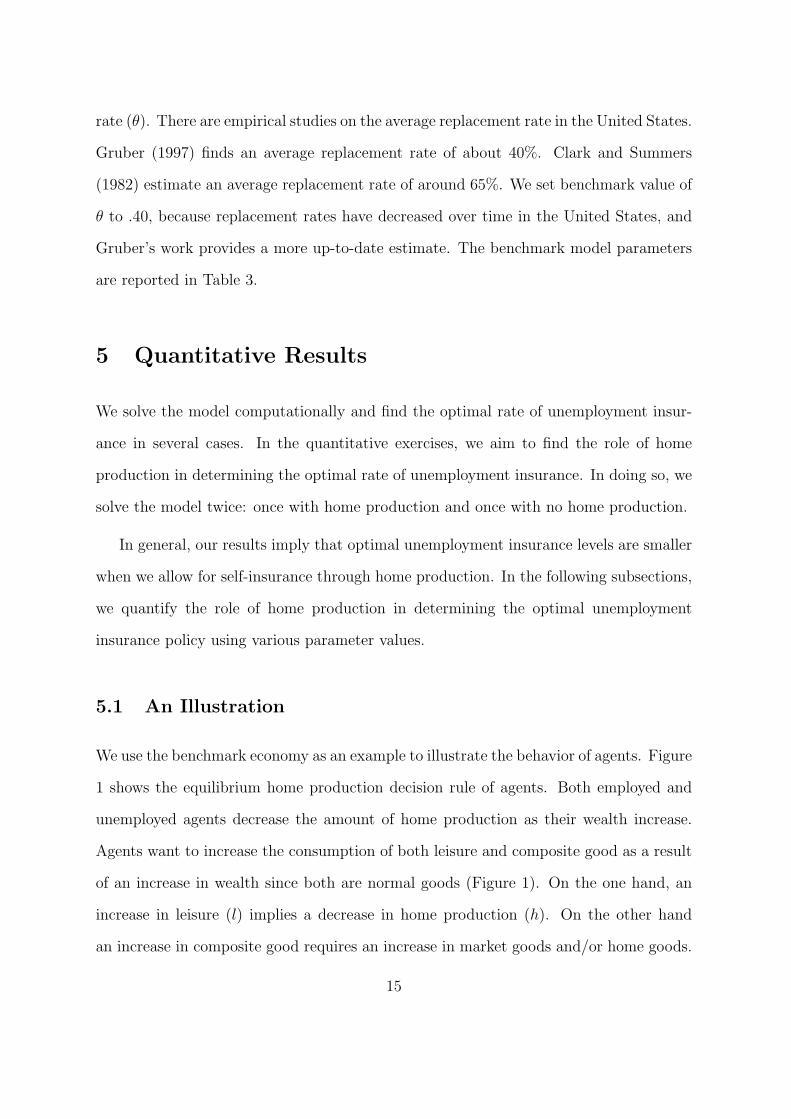
We use the benchmark economy as an example to illustrate the behavior of agents. Figure
1 shows the equilibrium home production decision rule of agents. Both employed and
unemployed agents decrease the amount of home production as their wealth increase.
Agents want to increase the consumption of both leisure and composite good as a result
of an increase in wealth since both are normal goods (Figure 1). On the one hand, an
increase in leisure (l) implies a decrease in home production (h). On the other hand
an increase in composite good requires an increase in market goods and/or home goods.
15

Increasing consumption of home goods requires a decrease in leisure, therefore it is more
costly in comparison with that of market good. Combining this additional cost with
the substitutability between market goods and home goods in the benchmark model
(e = 2.11, Table 1) lead agents to substitute towards market goods and decrease home
production (Figure 1) in response to an increase in wealth.21
5.2 Optimal Rate of Unemployment Insurance
In this subsection, we aim to quantify the role of home production in determining the
optimal rate of unemployment insurance. In order to do that, we solve the model twice:
once with no home production and once with home production.
No-home production case
In this case, where agents are not allowed to do home production, composite good is
assumed to be equal to the consumption of market goods. Using the benchmark pa-
rameterization, the optimal rate of unemployment insurance is computed as 74% of lost
earnings in this case (Figure 2).
In order to explore the dynamics behind the optimal rate of unemployment insurance,
we analyze the impact of marginal increments in unemployment benefits on the welfare
of employed and unemployed separately.
An increase in unemployment benefits always improves the welfare of unemployed due
to additional income at unemployment spells providing better consumption smoothing
(Figures 2,3).
Welfare of employed agents illustrates a hump-shape figure with respect to unem-
ployment benefits. It increases up to a threshold level, and decreases after then. On the
21See Guler and Taskin (2013) for a theoretical discussion on the correlation between wealth and homeproduction.
16

one hand, incremental unemployment benefits increase the welfare of employed through
their continuation value (welfare of unemployed). On the other hand, it reduces welfare
of employed because benefits are funded through income tax. The first effect dominates
up to the threshold and the second one dominates after then. This is reflected as a hump-
shape in Figure 2 (welfare of employed). Saving behavior of agents also determinant in
this threshold because marginal benefit of incremental unemployment insurance depends
on savings which is an additional insurance channel. When agents save sufficiently high,
the improvement through continuation value declines and first effect dominates (Figure
4)22
Home production case
In this case, we let agents to do home production as well as market production in the
model economy. Therefore, composite good is assumed to be a combination of home
production and market goods in this case. The optimal rate of unemployment insurance
is found to be 63% of lost earnings when we use benchmark parameters (Figure 5).
The difference between the two cases relies on the additional insurance channel
through home production. This is reflected as a significant improvement in relative
consumption of unemployed in the case of home production (Figure 3,7).
The mechanism in no-home production case works in this case as well. In particular,
an increase in unemployment benefits always improves the welfare of unemployed due
to additional income at unemployment spells providing better consumption smoothing
22Saving behavior of agents illustrate an interesting pattern when replacement rate is higher than70%. In this case, unemployed agents save more than employed. This happens due to the fact that com-posite consumption is a combination of leisure and consumption good. When replacement rate is high,consumption good is very well insured against unemployment shocks for employed agents. Therefore,the gap between employed and unemployed agents’ consumption is small in this case. However, for anunemployed agent, the risk of reduced leisure is not covered against an employment shock. As a result,unemployed agent saves more than employed in order to smooth the composite consumption betweenthe two states.
17

(Figure 5).
Congruous to the no-home production case, welfare of employed agents increases up to
a threshold level, and decreases after then. On the one hand, incremental unemployment
benefits increase the welfare of employed through their continuation value (welfare of
unemployed). On the other hand, it reduces welfare of employed because benefits are
funded through income tax. The first effect dominates up to the threshold and the
second one dominates after then. However, in this case, home production provides an
additional insurance channel, as well as savings, and this additional insurance channel
further decreases the marginal benefit through continuation value of employed agents.
Eventually, the threshold level of unemployment benefits ends up with a lower value in
home-production case. Similar to the case of no-home production, average savings are
responsive to the amount of unemployment benefits. This is affecting the optimal rate
of unemployment insurance because savings provide an additional insurance channel for
agents (Figure 8).
The relative consumption of unemployed in home production case is significantly
higher than that of no-home production case (Figure 3,7). The underlying mechanism
relies on the response of market good consumption and home production to the incre-
ments in unemployment benefits. As discussed in Section 5.1, agents are supposed to
increase their market good consumption and decrease their home production in response
to an increase in their disposable income. An increase in unemployment benefits in-
creases the disposable income of unemployed and decreases that of employed due to the
fact that increased unemployment benefits require higher income taxes. As an imme-
diate consequence, unemployed increase their market good consumption and decrease
their home production, and employed do the opposite when unemployment benefits are
increased (Figure 6).
As a consequence of the underlying additional insurance channel through home pro-
18

duction, the optimal rate of unemployment insurance is found to be significantly smaller
(63%) in comparison with the case where we close this channel (74%). In the next section,
we repeat the quantitative exercises with a variety of parameters to check robustness of
this result.
5.3 Sensitivity Checks
In this section, we repeat the quantitative experiment with various values of parameters
σ and ϕ. We keep the rest of the parameters at their benchmark value except α and e
which determine the average time spent for home production. For each value of σ and ϕ,
we recalibrate α and e to match unemployed and employed agents’ average time devoted
for home production. Moreover, we repeated the quantitative exercises with targeting
two broader definitions of home production and present the results in Table 4.
Relative risk aversion
The relative risk aversion parameter affects the decisions of agents in both home produc-
tion and no home production economies. Optimal θ changes significantly with respect
to σ in both economies. The mechanism works through savings. In both economies,
agents save more to smooth their consumption as they get more risk averse. Therefore
unemployment benefits become less necessary in comparison with the lower risk aversion
case. As expected, optimal θ falls in both cases. However, the difference between the
two cases is robust, as home production always provides an additional insurance channel
in the second economy (Table 4).
19

The value of leisure
The value of leisure is an important parameter in both economies because it affect the
relative value of consumption and the opportunity cost of home production. For smaller
values of ϕ, the importance of leisure in utility increase, and that of consumption de-
crease. Recall that unemployment benefit is valuable for agents because it provides
consumption smoothing. Therefore, as we decrease ϕ, the role of unemployment insur-
ance decreases in both economies. As a consequence, the optimal θ declines in both
economies. Again, the difference in optimal θ between the two economies is robust due
to the additional insurance through home production (Table 4).
Time spent for home production
In this section, we calculate the optimal rate of unemployment insurance using two
broader definitions of home production. First, we include the time spent for child care
and adult care to the definition of home production. This definition results in 30.29
hours/week for unemployed and 17.81 hours/week for employed. The optimal rate of
unemployment insurance decreases to 47% in this case. We also take the average of the
two definitions which results in 24.62 hours/week for unemployed and 14.03 hours/week
for employed. The optimal rate of unemployment insurance is computed as 57% in this
case. The rate of optimal unemployment insurance decreases as the average time spent
for home production increases due to the fact that the increase in home production
improves the amount of self-insurance through home production. The improvement in
self-insurance eventually leaves less room for public insurance through unemployment
benefits.
20

6 Conclusion
In this paper, we perform a quantitative analysis of optimal unemployment insurance,
where we incorporate self-insurance through home production and savings. Depending
on the definition of home production, we find that the optimal replacement rate is be-
tween 47% and 63% of wages, which is 11 to 27 percentage points lower than the no home
production model’s optimal replacement rate of 74%. The presence of home production
decreases the optimal replacement rate, and this result is robust under various param-
eterizations. The reason behind this result is the nature of the unemployment shock.
During unemployment spells, individuals have tighter constraints while purchasing mar-
ket goods and services and looser time constraints, and they respond by increasing their
home production against unemployment shocks. Since consumption is a function of home
goods and market goods, in the presence of home production, unemployed individuals
enjoy smoother consumption levels in comparison with the no-home production case.
Eventually, that lowers the optimal replacement rate significantly.
21

References
[1] Abdulkadiroglu, Atila, Burhanettin Kuruscu, and Aysegul Sahin (2002). “Unem-ployment Insurance and the Role of Self-Insurance,” Review of Economic Dynamics,5(3), 681-703.
[2] Acemoglu, Daron and Robert Shimer (1999), “Efficient Unemployment Insurance,”Journal of Political Economy, 107(5), 893-928.
[3] Acemoglu, Daron and Robert Shimer (2000), “Productivity Gains from Unemploy-ment Insurance,” European Economic Review, 44(7), 1195-1224.
[4] Aguiar, Mark and Erik Hurst (2005), “Consumption vs. Expenditure,” Journal ofPolitical Economy, 113(5), 919-948.
[5] Aguiar, Mark and Erik Hurst (2007), “Life-Cycle Prices and Production,” AmericanEconomic Review, 97(5), 1533-1559.
[6] Aguiar, Mark, Hurst, Erik, and Loukas Karabarbounis (2013), “Time Use DuringRecessions,” American Economic Review, forthcoming.
[7] Aiyagari, S. Rao (1994), “Uninsured Idiosyncratic Risk and Aggregate Saving,” TheQuarterly Journal of Economics, 109(3), 659-84.
[8] Alvarez-Parra, Fernando and Juan M. Sanchez (2010), “Unemployment Insurancewith a Hidden Labor Market,” Journal of Monetary Economics, 56(7), pp. 954-67.
[9] Bailey, Martin (1978), “Some Aspects of Optimal Unemployment Insurance,” Jour-nal of Public Economics, 10(3), 379-402.
[10] Becker, Gary (1965), “A Theory of The Allocation of Time”. The Economic Journal,75, 493-517.
[11] Becker, Gary D. and Gilbert R Ghez (1975), “The Allocation of Time and Goodsover the Life Cycle,” NBER.
[12] Benhabib, Jess, Richard Rogerson, and Randall Wright (1991), “Homework inMacroeconomics: Household Production and Aggregate Fluctuations,” Journal ofPolitical Economy, 99(6), 1166-87.
[13] Browning, Martin and Thomas Crossley (2001), “Unemployment Insurance BenefitLevels and Consumption Changes,” Journal of Public Economics, 80(1), 1-23.
[14] Burda, Michael C. and Daniel Hamermesh (2010), “Unemployment, Market Workand Individual Production,” Economics Letters, 107(2), 131-33.
[15] Canova, Fabio and Angel Ubide (1998), “International Business Cycles, FinancialMarkets, and Household Production,” Journal of Economic Dynamics and Control,22(4), 545-572.
22

[16] Carroll, Christopher, Karen Dynan, and Spencer Krane (2003), “UnemploymentRisk and Precautionary Wealth: Evidence From Households’ Balance Sheets,” TheReview of Economics and Statistics, 85(3), 586-604.
[17] Chang, Yongsung (2000), “Comovement, Excess Volatility, and Home Production,”Journal of Monetary Economics, 46(2), 385-396.
[18] Chang, Yongsung and Andreas Hornstein (2007), “Home Production,” Federal Re-serve Bank of Richmond, working paper.
[19] Chetty, Raj (2008), “Moral Hazard vs. Liquidity and Optimal Unemployment In-surance,” Journal of Political Economy, 116(2), 173-234.
[20] Clark, Kim B. and Lawrence H. Summers (1982), “Unemployment Insurance andLabor Market Transitions,” In Workers, Jobs, and Inflation, edited by Martin NeilBaily. Washington: Brookings Inst.
[21] Davidson, Carl and Stephen Woodbury (1997), “Optimal Unemployment Insur-ance,” Journal of Public Economics, 64(3), 359-387.
[22] Engen Eric and Jonathan Gruber (2001), “Unemployment Insurance and Precau-tionary Saving,” Journal of Monetary Economics, 47(3), 545-579.
[23] Flemming, J. S. (1978), “Aspects of Optimal Unemployment Insurance,” Journal ofPublic Economics, 10(3), 403-425.
[24] Greenwood, Jeremy and Zvi Hercowitz (1991), “The Allocation of Capital and Timeover the Business Cycle,” Journal of Political Economy, 99(6), 1188-214.
[25] Gruber, Jonathan (1997), “The Consumption Smoothing Benefits of UnemploymentInsurance,” The American Economic Review, 87(1), 192-205 .
[26] Gruber, Jonathan (2001), “The Wealth of Unemployed,” Industrial and Labor Re-lations Review, 55(1), 79-94.
[27] Guler, Bulent and Temel Taskin (2013), “Does unemployment insurance crowd outhome production?,” European Economic Review, Elsevier, vol. 62(C), pages 1-16.
[28] Hagedorn, Marcus, Ashok Kaul and Tim Mennel (2005), “An Adverse SelectionModel of Optimal Unemployment Insurance,” mimeo, Institute for Empirical Re-search in Economics, University of Zurich.
[29] Hamermesh, Daniel S., Harley Frazis and Jay Stewart, 2005. “Data Watch: TheAmerican Time Use Survey,” Journal of Economic Perspectives, American EconomicAssociation, 19(1), 221-232.
[30] Hansen, Gary and Ayse Imrohoroglu (1992), “The Role of Unemployment Insurancein an Economy with Liquidity Constraints and Moral Hazard,” Journal of PoliticalEconomy, 100(1), 118-42.
23

[31] Heathcote, Jonathan, Kjetil Storesletten and Giovanni Violante (2009), “Quanti-tative Macroeconomics with Heterogeneous Households,” Federal Reserve Bank ofMinneapolis, Staff Report.
[32] Hopenhayn, Hugo A. and Juan Pablo Nicolini (1997), “Optimal UnemploymentInsurance,” Journal of Political Economy, 105(2), 412-38.
[33] Jacobs, Kris (2007), “Consumption-Leisure Non-separabilities in Asset Market Par-ticipants’ Preferences,” Journal of Monetary Economics, 54(7), 2131-2138.
[34] Kocherlakota, Narayana R.,“Figuring out the impact of hidden savings on optimalunemployment insurance,” Review of Economic Dynamics, 2004, 7 (3), 541554.
[35] Krueger, Alan B. and Andreas Mueller (2010), “Job Search and UnemploymentInsurance: New Evidence from Time Use Data,” Journal of Public Economics, 94(3-4), 298-307.
[36] Kydland, Finn and Edward Prescott (1991), “Hours and Employment in BusinessCycle Theory,” Economic Theory, 1(1), 63-81.
[37] Landais, Camille, Pascal Michaillat and Emmanuel Saez (2010), “Optimal Unem-ployment Insurance over the Business Cycle,” working paper, NBER.
[38] Pallage, Stephane and Christian Zimmermann (2005), “Heterogeneous Labor Mar-kets and Generosity Towards Unemployed: An International Perspective,” Journalof Comparative Economics, 33(1), 88-106.
[39] Shavell, Steven and Laurence Weiss (1979), “The Optimal Payment of Unemploy-ment Insurance over Time,” Journal of Political Economy, 87(6), 1347-62.
[40] Shimer, Robert and Ivan Werning (2008), “Liquidity and Insurance for the Unem-ployed,” American Economic Review, 98(5), 1922-42.
[41] Wang, Cheng and Stephen D. Williamson, “Moral Hazard, Optimal UnemploymentInsurance, and Experience Rating,” Journal of Monetary Economics, 2002, 49 (7),1337-71.
24

7 Tables and Figures
Table 1: Summary Statistics (ATUS, 2003-2008)
Home production (narrow) Home production (broad) %Full Sample 13.14 22.48 100Unemployed 18.95 30.29 5Employed 11.13 19.49 65Full-time employed 10.24 17.81 49Not-in-labor force 20.05 32.92 30Single 10.40 16.81 42Married 14.58 25.45 58Female 16.38 28.42 52Male 9.80 16.33 48
Note: Unmarried couples are included in the “married” sample.
Table 2: Home Production and Unemployment in ATUS
Home production (narrow) Home productionUnemployed 8.924∗∗∗ 12.038∗∗∗
(0.511) (0.489)# of Obs. 53016 53016R2 0.081 0.122
Robust and clustered standard errors in parentheses∗∗∗ p < 0.001
25
Table 3: Parameters of the Benchmark Economy.
Parameter Valueβ Time discount factor .995σ Relative risk aversion 2.50ϕ Weight of leisure in utility .67n Constant labor supply .36θ Benchmark unemployment benefit .40
χ(0, 0) Unemployment/employment transition .50χ(1, 1) Employment/employment transition .9681
s Elasticity of substitution b/w market goods and HP 1.32α Share of market goods in composite good .53
Table 4: Sensitivity Checks
Risk aversion (σ) Value of leisure (ϕ) Home production
1.5 2 2.5 3 4 .20 .25 .33 .40 .50 .60 HP1 HP2 HP3θ, HP .79 .69 .63 .57 .50 .31 .50 .63 .70 .78 .83 .63 .57 .47
θ, no HP .88 .81 .74 .70 .64 .66 .71 .74 .78 .83 .87 .74 .74 .74Dif. .09 .12 .11 .13 .14 .35 .21 .11 .08 .05 .05 .11 .17 .27
Notes: This table shows the summary of our sensitivity checks. HP1 and HP3 denote thenarrow and broad definition of home production, respectively. HP2 is the average of the two.
26

Table 5: Optimal rate of unemployment insurance
θ τ v vu ve a au ae c cu ce0.05 0.003 -3099.97 -3110.33 -3099.31 2.48 1.54 2.54 0.94 0.552 0.9650.10 0.006 -3098.99 -3107.68 -3098.44 2.07 1.22 2.12 0.94 0.553 0.9650.15 0.009 -3098.04 -3105.14 -3097.58 1.72 0.96 1.77 0.94 0.554 0.9650.20 0.013 -3097.12 -3102.70 -3096.76 1.42 0.75 1.47 0.94 0.557 0.9640.25 0.016 -3096.21 -3100.33 -3095.95 1.16 0.57 1.20 0.94 0.559 0.9640.30 0.019 -3095.35 -3098.05 -3095.18 0.93 0.43 0.96 0.94 0.562 0.9640.35 0.022 -3094.53 -3095.87 -3094.44 0.72 0.30 0.75 0.94 0.566 0.9640.40 0.025 -3093.71 -3093.73 -3093.71 0.55 0.20 0.57 0.94 0.572 0.9640.45 0.028 -3092.97 -3091.73 -3093.05 0.39 0.12 0.41 0.94 0.578 0.9630.50 0.031 -3092.22 -3089.76 -3092.38 0.26 0.07 0.27 0.94 0.587 0.9630.55 0.034 -3091.56 -3087.94 -3091.79 0.15 0.03 0.16 0.94 0.597 0.9620.60 0.037 -3090.91 -3086.19 -3091.21 0.07 0.01 0.07 0.94 0.612 0.9610.65 0.040 -3090.32 -3084.60 -3090.68 0.02 0.00 0.02 0.94 0.633 0.9600.70 0.043 -3089.82 -3083.25 -3090.23 0.00 0.00 0.00 0.94 0.670 0.9570.75 0.046 -3089.66 -3082.37 -3090.13 0.00 0.00 0.00 0.94 0.714 0.9540.80 0.049 -3089.74 -3081.56 -3090.26 0.01 0.07 0.00 0.94 0.728 0.9540.85 0.051 -3089.86 -3080.78 -3090.44 0.02 0.15 0.01 0.94 0.736 0.9530.90 0.054 -3090.01 -3080.03 -3090.65 0.04 0.25 0.03 0.94 0.742 0.9530.95 0.057 -3090.19 -3079.32 -3090.88 0.06 0.34 0.04 0.94 0.747 0.952
Notes: This table shows the summary of our quantitative results on the optimal unem-ployment insurance policy: no-home production case. The notations θ, τ , v, a, and crepresent replacement rate, tax rate, welfare, saving, and consumption respectively. Thesubscripts u, and e represent unemployed and employed respectively. Lastly, x representsthe mean of x.
27

Table 6: Optimal rate of unemployment insurance: home production case
θ τ v vu ve h hu he
0.05 0.003 -391.64 -391.69 -391.64 0.0962 0.172 0.09140.1 0.006 -391.56 -391.48 -391.57 0.0962 0.172 0.09140.15 0.009 -391.49 -391.29 -391.50 0.0962 0.171 0.09140.2 0.013 -391.42 -391.10 -391.44 0.0962 0.171 0.09140.25 0.016 -391.35 -390.92 -391.38 0.0962 0.171 0.09140.3 0.019 -391.29 -390.74 -391.32 0.0961 0.170 0.09140.35 0.022 -391.22 -390.57 -391.27 0.0961 0.170 0.09140.4 0.025 -391.17 -390.41 -391.21 0.0961 0.169 0.09140.45 0.028 -391.11 -390.26 -391.16 0.0961 0.168 0.09140.5 0.031 -391.06 -390.12 -391.12 0.0960 0.168 0.09140.55 0.034 -391.01 -389.99 -391.08 0.0960 0.167 0.09150.6 0.037 -390.98 -389.89 -391.05 0.0959 0.165 0.09150.65 0.040 -390.98 -389.82 -391.05 0.0959 0.163 0.09150.7 0.043 -390.98 -389.76 -391.06 0.0958 0.163 0.09160.75 0.046 -390.99 -389.69 -391.08 0.0958 0.163 0.09160.8 0.049 -391.01 -389.63 -391.09 0.0958 0.163 0.09160.85 0.051 -391.02 -389.56 -391.11 0.0958 0.162 0.09160.9 0.054 -391.04 -389.51 -391.13 0.0958 0.162 0.09160.95 0.057 -391.05 -389.45 -391.15 0.0958 0.162 0.0916
θ a au ae cm ¯cmu ¯cme c cu ce0.05 1.69 0.95 1.73 0.94 0.44 0.97 0.368 0.29 0.3730.1 1.36 0.71 1.40 0.94 0.44 0.97 0.368 0.29 0.3730.15 1.09 0.53 1.13 0.94 0.45 0.97 0.368 0.29 0.3730.2 0.86 0.38 0.89 0.94 0.45 0.97 0.368 0.29 0.3730.25 0.66 0.26 0.68 0.94 0.46 0.97 0.368 0.29 0.3730.3 0.48 0.17 0.50 0.94 0.46 0.97 0.368 0.29 0.3730.35 0.34 0.10 0.35 0.94 0.47 0.97 0.368 0.30 0.3730.4 0.21 0.05 0.22 0.94 0.48 0.97 0.368 0.30 0.3720.45 0.12 0.02 0.12 0.94 0.49 0.97 0.368 0.31 0.3720.5 0.04 0.00 0.05 0.94 0.51 0.97 0.368 0.31 0.3720.55 0.00 0.00 0.00 0.94 0.53 0.97 0.368 0.32 0.3720.6 0.00 0.00 0.00 0.94 0.58 0.96 0.369 0.33 0.3710.65 0.00 0.03 0.00 0.94 0.61 0.96 0.369 0.34 0.3700.7 0.01 0.10 0.01 0.94 0.62 0.96 0.369 0.35 0.3700.75 0.03 0.19 0.02 0.94 0.63 0.96 0.369 0.35 0.3700.8 0.05 0.28 0.03 0.94 0.63 0.96 0.369 0.35 0.3700.85 0.07 0.38 0.05 0.94 0.64 0.96 0.369 0.35 0.3700.9 0.09 0.48 0.06 0.94 0.64 0.96 0.369 0.35 0.3700.95 0.12 0.58 0.09 0.94 0.65 0.96 0.369 0.36 0.370
Notes: This table shows the summary of our quantitative results on the optimal unemploymentinsurance policy: home production case. The notations θ, τ , v, h, a, cm, and c representreplacement rate, tax rate, welfare, home production, saving, market good consumption, andcomposite good consumption respectively. The subscripts u, and e represent unemployed andemployed respectively. Lastly, x represents the mean of x.
28

0 2 4 6 8 100.2
0.3
0.4
0.5Composite good consumption
0 2 4 6 8 100.825
0.83
0.835
0.84
0.845
0.85
0.855Leisure
0 2 4 6 8 100.2
0.4
0.6
0.8
Wealth
Market good consumption
0 2 4 6 8 100.8
1
1.2
1.4
0 2 4 6 8 100.155
0.16
0.165
0.17
0.175Home production
0 2 4 6 8 100.086
0.088
0.09
0.092
0.094
0 2 4 6 8 100.548
0.549
0.55
0.551
0.552
0.553
0.554
0 2 4 6 8 100.35
0.4
0.45
0.5
UnemployedEmployed−right axis
Figure 1: Decision rules.
0 0.5 1−796
−794
−792
−790
−788
−786
Unemployment benefits
Welfare
Unemployed
0 0.5 1−792
−791.5
−791
−790.5
−790
−789.5
−789Employed
0 0.5 1−792
−791.5
−791
−790.5
−790
−789.5
−789Aggregate
Figure 2: Unemployment benefits versus aggregate welfare: no home production case.
29

0 0.2 0.4 0.6 0.8 10.55
0.6
0.65
0.7
0.75
0.8
Unemployment benefits
Relative consumption of unemployed
0 0.2 0.4 0.6 0.8 10.55
0.6
0.65
0.7
0.75Consumption
0 0.2 0.4 0.6 0.8 10.95
0.955
0.96
0.965
0.97
UnemployedEmployed−right axis
Figure 3: Unemployment benefits versus consumption: no home production case.
0 0.1 0.2 0.3 0.4 0.5 0.6 0.7 0.8 0.9 10
0.5
1
1.5
2
2.5
3
Unemployment benefits
Savings
UnemployedEmployed
Figure 4: Unemployment benefits versus saving: no home production case.
30

0 0.5 1−392
−391.5
−391
−390.5
−390
−389.5
−389
Unemployment benefits
Welfare
Unemployed
0 0.5 1−391.8
−391.7
−391.6
−391.5
−391.4
−391.3
−391.2
−391.1
−391Employed
0 0.5 1−391.8
−391.6
−391.4
−391.2
−391
−390.8Aggregate
Figure 5: Unemployment benefits versus welfare: home production case.
0 0.2 0.4 0.6 0.8 10.4
0.5
0.6
0.7Market good consumption
0 0.2 0.4 0.6 0.8 10.162
0.164
0.166
0.168
0.17
0.172
0.174
Unemployment benefits
Home production
0 0.2 0.4 0.6 0.8 10.0913
0.0914
0.0914
0.0915
0.0915
0.0916
0.0916
0 0.2 0.4 0.6 0.8 10.95
0.96
0.97
0.98
UnemployedEmployed−right axis
Figure 6: Unemployment benefits versus home production and market good consump-tion.
31

0 0.2 0.4 0.6 0.8 10.28
0.3
0.32
0.34
0.36
0.38Consumption
0 0.2 0.4 0.6 0.8 10.75
0.8
0.85
0.9
0.95
1
Unemployment benefits
Relative consumption of unemployed
0 0.2 0.4 0.6 0.8 10.369
0.37
0.371
0.372
0.373
0.374
UnemployedEmployed−right axis
Figure 7: Unemployment benefits versus relative consumption of unemployed: homeproduction case.
0 0.1 0.2 0.3 0.4 0.5 0.6 0.7 0.8 0.9 10
0.2
0.4
0.6
0.8
1
1.2
1.4
1.6
1.8
Unemployment benefits
Savings
UnemployedEmployed
Figure 8: Unemployment benefits versus saving: home production case.
32