Optimal Earnings-Related Unemployment Benefits*

Mohammad Taslimi* April 2003

Abstract

Existing unemployment insurance systems in many OECD countries involve a ceiling on

insurable earnings. The result is lower replacement rate for employees with relatively high

earnings. This paper examines whether replacement rates should decrease as the level of

earnings rises. The framework is a search equilibrium model where wages are determined by

Nash bargaining between firms and workers, job search intensity is endogenous and workers

are heterogeneous. The analysis suggests higher replacement rates for low-paid workers if

taxes are uniform. The same result may hold when taxes are redistributive. Numerical

simulations indicate that there are modest welfare gains associated with moving from an

optimal uniform benefit system to an optimally differentiated one in both cases, i.e., uniform

and redistributive taxation. The case for differentiation arises from the fact that it may have

favourable effects on the tax base.

Keywords: Unemployment Insurance, Unemployment, Search. JEL-Classification: D81, D83, J64, J65.

* I am grateful to Peter Fredriksson, Nils Gottfries, Bertil Holmlund and Juhana Vartiainen for useful comments and suggestions. Thanks also to Per Engström for valuable help with the programming. The author bears full responsibility for all potential errors. * Department of Economics, Uppsala University, Box 513, SE-751 20 Uppsala, Sweden. E-mail: mohammad.taslimi@nek.uu.se

1

1. Introduction

The process of industrialization created new kinds of risks such as mass unemployment and

income uncertainty. The uncertain employment prospects together with risk averse individuals

resulted in the provision of unemployment insurance (UI) in order to mitigate the risks.1While

the earliest forms of UI were developed by trade unions in Great Britain in 1832, France was

the first state providing this kind of social protection in 1905.

However, there are other reasons except demand for income security behind the public

provisions of UI. Unemployment benefits enable the unemployed person to spend sufficient

time to search for a job that matches his skill level, whereas lack of income can force the

unemployed to take a job which does not match his skill. In this case the existence of UI

increases labour market efficiency and reduces the cost of search for the unemployed.

Moreover, improved matching of workers to vacant jobs may reduce the probability of future

spells of unemployment. At the same time, employers are likely to find it easier to dismiss

workers under a UI regime, since workers will tend to demand less compensation for losing

jobs. It will allow employers to adopt methods of production with higher risk of redundancy.

In addition, the willingness of workers to be mobile is likely to be greater under a UI regime.

However, UI may have adverse incentive effects. More generous UI benefits may increase

unemployment by reducing search effort2and/or increasing wage pressure.3 On the other hand,

the existence of insurance schemes increases the incentive for uninsured to find employment

in order to become eligible for future benefits.4 But this entitlement effect may imply that the

unqualified individuals accept the first offered job that does not match their skill.

From a social perspective, an effective system of income protection for the unemployed

reduces divisions in society and provides some form of justice to people who lose their jobs

through no fault of their own; from a macroeconomic perspective, it stabilises purchasing

power and so the demand for goods and services.

Despite these facts protection against the financial risk of unemployment developed later than

provision for other circumstances5 (industrial accident, old age pension, health, and family

1 Agell (2000). 2 See Baily (1978), Flemming (1978), Shavell and Weiss (1979). 3 Johnson and Layard (1986). 4 Mortensen (1977). 5 Alber (1981), Alber and Flora (1981), Flora (1987) and Tsukada (2002).

2

allowance). However, UI is now not only an integral part of the social welfare system, it is

also one of the most important institutions of social insurance in most advanced economies.

Over the past couple of decades, a considerable amount of work has been devoted to the

economic analysis of the impact of unemployment benefits on unemployment. Since the

emergence of job-search theory6, economists have got an effective analytical tool for labour

market analysis. This has resulted in a large amount of theoretical and empirical research.

Today, although the theory of job search7 is a young actor on the stage of labour market

analysis, it plays a major part in the economics of labour. It may be one of the reasons that

labour economics and the institutions and rules that govern labour markets have moved from

the periphery to the centre of economic discourse.8

Another reason behind the considerable attention in research about UI benefit systems, and

the most important reason in my opinion, is the rise in unemployment in the most OECD

countries during the 1970s, 1980s, and 1990s and its persistence in most countries. In the

European union there are about 27 million people unemployed or would be willing to sign up

for a job if labour market prospects improved. Furthermore, half of the unemployed has been

out of work for more than one year.9

Various aspects have been explored e.g. the relationship between benefit levels and the

duration of unemployment, the impact of benefit duration on unemployment duration, and the

linkages between UI through job search and labour supply.10 Put differently, there has been a

considerable attention to explore rational individual behaviour during unemployment.

However, there are still areas that have not been developed. Despite the voluminous literature

on this topic, there is in fact relatively little attention paid to the relationship between the

structure of UI benefit system and unemployment. The following analysis is a first step

towards a theoretical evaluation of this aspect.

6 A rigorous and detailed analysis of the impact of UI on individual job search behaviour under imperfect information was first provided by Dale Mortensen (1977). 7 Another key feature of the theory is that it tries to describe the behaviour of unemployed individuals in a dynamic, ever changing and uncertain environment since the certain and static environments used by previous models could not represent many of life’s real work experiences. 8 See Freeman (1998). 9 See Munzi and Salomäki (1999). 10 For a more detailed discussion of the development of UI in theory and practice see Holmlund (1998), Devine and Kiefer (1991) and Atkinson and Mickelwright (1991).

3

All OECD countries have schemes for the specific purpose of paying benefits to unemployed

persons, and even though these schemes differ widely from one country to another, the benefit

level in most countries has a maximum. Income support for workers is usually based on one

of two principles (or both): insurance or assistance. Assistance payments, available to

unemployed that are not qualified for insurance benefit, are usually not related to past

contributions, though they may vary with age, marital status and number of children.

The insurance-type schemes are quite often unrelated to family circumstances and generally

related to previous earnings in employment and based on one of two principles: either the

amount of benefit is fixed on a flat-rate basis (Beveridgean); or it is proportional to the wage

(Bismarckian).11 While most countries in EU have wage-related UI benefit system, the UK

has flat-rate benefit system since 1982. In practice, however, compensation schemes can

involve both principles. At the same time, a ceiling imposed on benefits can substantially

reduce the proportion of previous income received. This paper focuses on this aspect of

earnings-related benefits schemes.

The aim of the paper is to analyse the optimal structure of replacement rates in a search

equilibrium framework along the lines of Pissarides (2000). The model allows for endogenous

search effort among unemployed workers. Wages are assumed to be endogenous as in

Fredriksson and Holmlund (2001), but benefit payments are indefinite, which means that

there is no risk of loosing benefits for unemployed workers. There are two types of workers,

where one type is more productive and therefore receives a higher wage. Furthermore,

replacement rates are allowed to be different. We find that the optimal system is characterised

by lower replacement rates for workers with higher wages if taxes are uniform. In the case of

redistributive taxation, the same result may hold under certain condition.

The paper is organised as follows. Section 2 provides an overview of the system of

unemployment insurance in the OECD countries. Section 3 is devoted to the presentation of

the model. Section 4 derives some analytical results concerning the properties of the optimal

replacement rates. In section 5 of the paper I present the numerical results concerning the

optimal replacement rates and finally, section 6 concludes.

11 OECD (1999).

4

2. Earnings-Related UI in Practice

Within the OECD the replacement rates for unemployed vary substantially. The designs of UI

reflect national values and norms. Each country has built its own system with its own specific

national features, and there is not any common form of UI system in OECD countries. The

regulation of unemployment insurance is often very complicated. These facts make it difficult

to rank the systems according to some criteria.

Generally, a minimum period of insured employment is required to qualify for UI benefits.

This period ranges from 10.5 weeks in Canada to 108 weeks in Portugal. The initial rate of

benefit ranges from 40 to 90 percent of previous earnings. The benefit rate is related to gross

earnings with the exception of Germany, where the payment rates are expressed as a

percentage of net income. UI benefits are taxed in most countries but not in Germany,

Australia, Austria, Czech Republic, Japan, Korea, Portugal and the United Kingdom. Only in

Belgium is UI unlimited in duration. Payment rates decrease over time in several countries,

e.g. Belgium, Czech Republic, France, Hungry and Norway. The payment rates can depend

on age, family situation, employment record and previous earnings.12 However, despite the

complexity and diversity of national unemployment insurance arrangements13 that results in a

wide diversity in coverage and organisation of UI,14 there are some common characteristics

shared across countries in OECD.

Unemployment insurance schemes are generally of a compulsory nature for the majority of

countries, with Denmark and Sweden as exceptions. Furthermore, the state is involved in

establishing the regulation of UI schemes, although government participation in financing

insurance schemes differs a great deal from one country to another.

12 OECD (1999). 13 Unemployment insurance differs, like social insurance, even between most advanced economies. Esping-Andersen (1990) discusses three different types of welfare capitalism in 18 advanced economies with three types of social policy regimes. Leibfried (1993) found a fourth type including Portugal, Spain and Greece. Historically, there are also differences between these countries about the establishment and development of the welfare state. While the German social insurance system had established by Chancellor Otto von Bismarck in the 1880s, the passage of the Social Security Act as a result of president Franklin D. Roosevelt’s New Deal in 1935 launched the American federal welfare state. See Leman (1980) and Brooks (1893). 14 A comparison of different studies about net replacement rates of the unemployed in EU countries shows that there are three similar groups of countries with high, intermediate and low replacement rates. The high replacement rates are noticed in Denmark, Finland, France, Luxembourg, Netherlands, Portugal and Sweden, the intermediate one in Austria, Belgium, Germany, Spain and United Kingdom and the low one in Greece, Ireland and Italy. Note that these studies are about the “net” rate of unemployment benefits where taxes and family-related benefits are included. See Munzi and Salomäki (1999).

5

Finally, the general character of the UI schemes in most OECD countries is that they contain

income-related benefits, i.e., the level of benefit paid is at least partially earnings-related in

most OECD countries. The exceptions are Iceland, Ireland, Korea, Poland and the United

Kingdom, where benefits are unrelated to previous income.15

Thus, either there is a ceiling on insurable earnings, as in most OECD countries, which fixes

the insurance benefit at the same level for a large proportion of the unemployed; or the

amount of benefit is fixed on a flat-rate basis. The latter point means that unemployment

insurance rarely operates as a pure insurance scheme. There is some major deviation from the

basic principles of insurance. One reason is presumably that there is a desire to introduce

some redistribution within the group of insured individuals. Such redistribution, which

depends on criteria other than the occurrence of the risk insured against, is typically to the

advantages of the low paid workers. Of course, redistribution within insurance schemes

differs substantially from one country to another and sometimes the differences are so great

between countries that it is scarcely possible to classify them in the same group.

Table 1 shows that the existing UI in many OECD countries involves an upper limit or ceiling

on insurable earnings. There is a fixed compensation rate up to a certain income level; above

this level, the maximum, benefits are fixed. This means that the actual replacement rate is

lower for employees with earnings exceeding the maximum level16; this rate can be much

lower than the maximum rates.17 Put another way, the wage replacement rate decreases as the

level of earnings rises. As a corollary some proportion of the unemployed receive the UI

benefit at the same level.

This fact creates some interesting questions that appear to have received little or no attention

in the economic literature. What is the optimal structure of replacement rates in a world with

heterogeneous labour? Consider an economy with two types of workers, one more productive

and therefore with higher wage. Should these two types have the same replacement rate or

15 There are some other common features in addition to these characteristics. One of the fundamental characteristics of social insurance, including unemployment insurance, is that it promotes solidarity principle, i.e., unlike private insurance, UI is a pooling of risks without differentiating contributions according to exposure to risk. Moreover, the state, employers and workers finance generally UI. 16 In Sweden, for example, 75 percent of all full-time employees had an income above the ceiling in 1996. See SOU (1996). 17 According to SOU (1996), employees with monthly earnings exceeding 25000 SEK in 1996 had a replacement rate lower than 50 percent of the lost income.

6

should one type have a higher benefit level? Is it possible to rationalise the empirical pattern

we observe, i.e., a system where low-income workers have higher replacement rates? Can

such a system be rationalised on efficiency grounds? Or do we need to invoke distribution

arguments?

Table 1. UI Systems Around the World

Replacement Rate (%) Maximum Benefit

Australia _ _

Austria 57 Yes

Belgium 60 Yes

Canada 55 Yes

Czech Republic 60 Yes

Denmark 90 Yes

Finland 90 Yes

France 75 Yes

Germany 60 Yes

Greece 40 Yes

Hungry 65 Yes

Iceland Flat Yes

Ireland Flat Yes

Italy 80 Yes

Japan 80 Yes

Korea Flat Yes

Luxembourg 80 Yes

Netherlands 70 Yes

New Zealand _ _

Norway 62.4 Yes

Poland Flat Yes

Portugal 65 Yes

Spain 70 Yes

Sweden 80 Yes

Switzerland 70 Yes

United Kingdom Flat Yes

United States 50 Yes

Notes: Australia and New Zealand have an assistance type benefit with characteristics of both unemployment assistance and social assistance.

Source: OECD (1999).

7

3. The Framework of Analysis

3.1 The Labour Market

Consider an economy with two separate sectors, indexed 2,1=i . One sector ( )1=i employs

exclusively workers with relatively low productivity; the other sector ( )2=i employs workers

with high productivity. There is no search on the job since we assume homogenous workers in

each sector and therefore no wage differentials within sectors. The total number of workers is

fixed and normalised to unity in each sector.

The number of jobs is variable and determined by zero-profit conditions. Firms produce

according to a constant returns to scale technology. As usual, we simplify by focusing on

“small” firms with only one job. At any point in time, a fraction iu−1 of the labour force in

sector i is employed while the remaining fraction iu is unemployed and searching for a job.

There is a continuum of infinitely- lived individuals, and time is continuous.

Existing jobs are destroyed at the exogenous Poisson rate iφ . This creates an inflow into the

unemployment pool that is equal to the outflow in equilibrium. There are frictions in the

labour market that make it impossible for all unemployed workers to find jobs

instantaneously.18

Unemployed workers are immediately eligible for UI benefits when they enter unemployment

and benefit payment is indefinite. These assumptions are made for tractability. Benefits are

provided by the government and are funded by taxing all workers’ incomes, both employed

and unemployed.

Let is denote search intensity. Thus, the effective number of searchers in a sector is given by

iii usS = . The matching function, which captures the frictions in the market, relates the flow

of new hires, iH , to the number of effective searchers and the number of vacant jobs, iv , i.e.,

),( iii vSHH = . It is assumed increasing in both its arguments, continuously differentiable,

concave, and homogenous of degree one.19

18 The sources of the frictions are costs and time delays, associated with imperfect information about the location of job and job characteristics, in the process of finding trading partners. 19 Empirical research suggests also a constant returns matching technology (see Petrongolo and Pissarides (2001)).

8

Let iii Sv /≡θ denote labour market tightness and ( ) ( ) ( )1,/1/, iiiiiii HvvSHq θθ ==

denote the rate at which vacant jobs become filled, so ( )iq θ/1 is the expected time until a

vacant job will be filled. Further, by the properties of matching technology, ( ) 0<′ iq θ : the

tighter the labour market, the more difficult for a firm to fill a vacancy. Fina lly, the elasticity

of ( )iq θ is denoted by ( ) ( )iii qq θθθσ /′−≡ , where ( )1,0∈σ .

Unemployed workers enter employment at the endogenous rate ( ) ( ) iiiiiiiii usvusHss /,=θα

and ( ) ( ) ( )iiiiiiiii HusvusH θθα ,1/, == , where. Moreover, ( ) ( ) ( ) 01 >−=′ ii q θσθα . Thus

the more vacancies the easier for workers to find jobs and the more unemployed workers the

easier for firms to fill their vacancies. In steady state the flow into unemployment equals the

flow out of unemployment. Thus, flow equilibrium implies ( ) ( )iiiii uus −= 1φθα which can

be rewritten as follows

( )iii

ii s

uθαφ

φ+

= 2,1=i (1)

Equation (1) is one of the key equations of the model. It implies a negative relationship

between search effort and unemployment rate. The other source of variation in unemployment

is iθ , which can be seen as a measure of labour market conditions.

3.2 The Behaviour of Workers

The two types of workers are matched in two separate labour markets. The employed workers

can affect the equilibrium outcome because they bargain over the wage rate. The unemployed

workers can influence the exit rate to employment and equilibrium unemployment through

their search effort. Workers have utility functions that are strictly concave in wage income

( )iw and leisure. The instantaneous utility of unemployed workers is decreasing in search

effort, since search reduces available leisure time. The utility function for the employed

worker is ( ) ( )iiii whw υυ =, , where h , hours of work, is exogenously fixed. The unemployed

workers utility is given by ( )iii sB ,=υ , where iB is the benefit level. The worker’s utility

function is assumed to be logarithmic:

9

iii c llnln γυ += 2,1=i (2)

where ic denotes consumption and il leisure. Workers do not have access to a capital

market, so consumption equals income at each instant. Let T denotes available time and iτ

the tax rate, thus, the consumption and leisure in the two states are given by )1( iii wc τ−=

and hTi −=l if employed; )1( iii Bc τ−= and ii sT −=l if unemployed. Thus, the

employed worker’s time is divided between work and leisure, whereas the unemployed

worker’s time is divided between search and leisure. The utility function can be rewritten as:

( ) ( )hTw iiei −+−= ln1ln γτυ and ( ) ( )iiii

ui sTwb −+−= ln1ln γτυ , where superscripts e and

u refer to employed and unemployed. We have assumed iii wbB = , where ib is the

replacement rate. Thus benefit levels are indexed to (average) wages within each sector.

The value functions can now be defined. Let iE and iU be the expected present values of

employment and unemployment, respectively, and let r denote the subjective rate of time

preference. Thus, the value functions can be written as follows:

( )iiieii UErE −−= φυ (3)

( )( )iiiiuii UEsrU −+= θαυ (4)

The unemployed worker chooses search effort to maximise the value of unemployment. The

first-order condition takes the form:

( ) 0=−+−

−≡Ψ iii

UEsT

αγ

(5)

where

( )( ) ( ) ( ) ( )

( )iii

iiiiii

iii

ui

ei

ii srsTwbhTw

srUE

θαφγτγτ

θαφυυ

++−−−−−+−

=++−

=−ln1lnln1ln

(6)

10

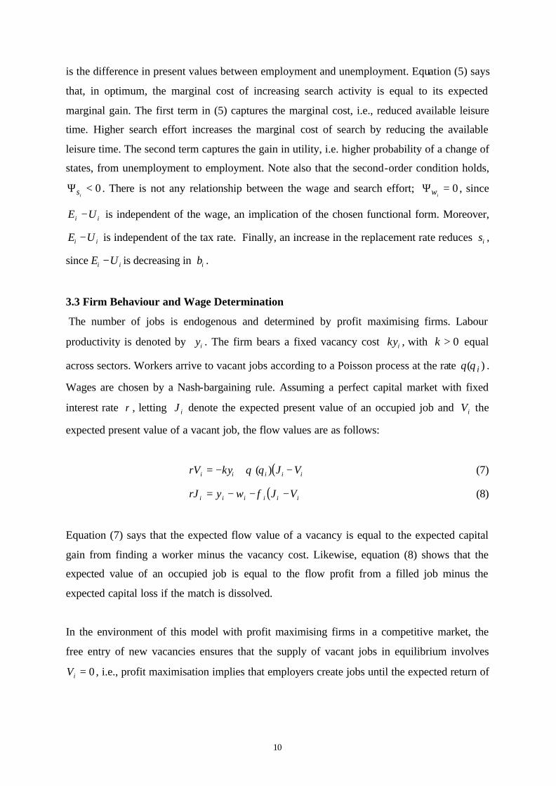
is the difference in present values between employment and unemployment. Equation (5) says

that, in optimum, the marginal cost of increasing search activity is equal to its expected

marginal gain. The first term in (5) captures the marginal cost, i.e., reduced available leisure

time. Higher search effort increases the marginal cost of search by reducing the available

leisure time. The second term captures the gain in utility, i.e. higher probability of a change of

states, from unemployment to employment. Note also that the second-order condition holds,

0<Ψis . There is not any relationship between the wage and search effort; 0=Ψ

iw , since

ii UE − is independent of the wage, an implication of the chosen functional form. Moreover,

ii UE − is independent of the tax rate. Finally, an increase in the replacement rate reduces is ,

since ii UE − is decreasing in ib .

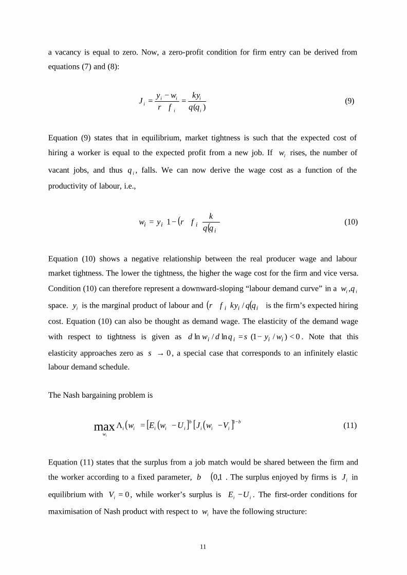
3.3 Firm Behaviour and Wage Determination

The number of jobs is endogenous and determined by profit maximising firms. Labour

productivity is denoted by iy . The firm bears a fixed vacancy cost iky , with 0>k equal

across sectors. Workers arrive to vacant jobs according to a Poisson process at the rate )( iq θ .

Wages are chosen by a Nash-bargaining rule. Assuming a perfect capital market with fixed

interest rate r , letting iJ denote the expected present value of an occupied job and iV the

expected present value of a vacant job, the flow values are as follows:

( )iiiii VJqkyrV −+−= )(θ (7)

( )iiiiii VJwyrJ −−−= φ (8)

Equation (7) says that the expected flow value of a vacancy is equal to the expected capital

gain from finding a worker minus the vacancy cost. Likewise, equation (8) shows that the

expected value of an occupied job is equal to the flow profit from a filled job minus the

expected capital loss if the match is dissolved.

In the environment of this model with profit maximising firms in a competitive market, the

free entry of new vacancies ensures that the supply of vacant jobs in equilibrium involves

0=iV , i.e., profit maximisation implies that employers create jobs until the expected return of

11

a vacancy is equal to zero. Now, a zero-profit condition for firm entry can be derived from

equations (7) and (8):

)( i

i

i

iii q

kyr

wyJ

θφ=

+−

= (9)

Equation (9) states that in equilibrium, market tightness is such that the expected cost of

hiring a worker is equal to the expected profit from a new job. If iw rises, the number of

vacant jobs, and thus iθ , falls. We can now derive the wage cost as a function of the

productivity of labour, i.e.,

( ) ( )

+−=

iiii q

kryw

θφ1 (10)

Equation (10) shows a negative relationship between the real producer wage and labour

market tightness. The lower the tightness, the higher the wage cost for the firm and vice versa.

Condition (10) can therefore represent a downward-sloping “labour demand curve” in a iiw θ,

space. iy is the marginal product of labour and ( ) ( )iii qkyr θφ /+ is the firm’s expected hiring

cost. Equation (10) can also be thought as demand wage. The elasticity of the demand wage

with respect to tightness is given as 0)/1(ln/ln <−= iiii wydwd σθ . Note that this

elasticity approaches zero as 0→σ , a special case that corresponds to an infinitely elastic

labour demand schedule.

The Nash bargaining problem is

( ) ( )[ ] ( )[ ] ββ −−−=Λ 1max iiiiiiiiw

VwJUwEwi

(11)

Equation (11) states that the surplus from a job match would be shared between the firm and

the worker according to a fixed parameter, ( )1,0∈β . The surplus enjoyed by firms is iJ in

equilibrium with 0=iV , while worker’s surplus is ii UE − . The first-order conditions for

maximisation of Nash product with respect to iw have the following structure:

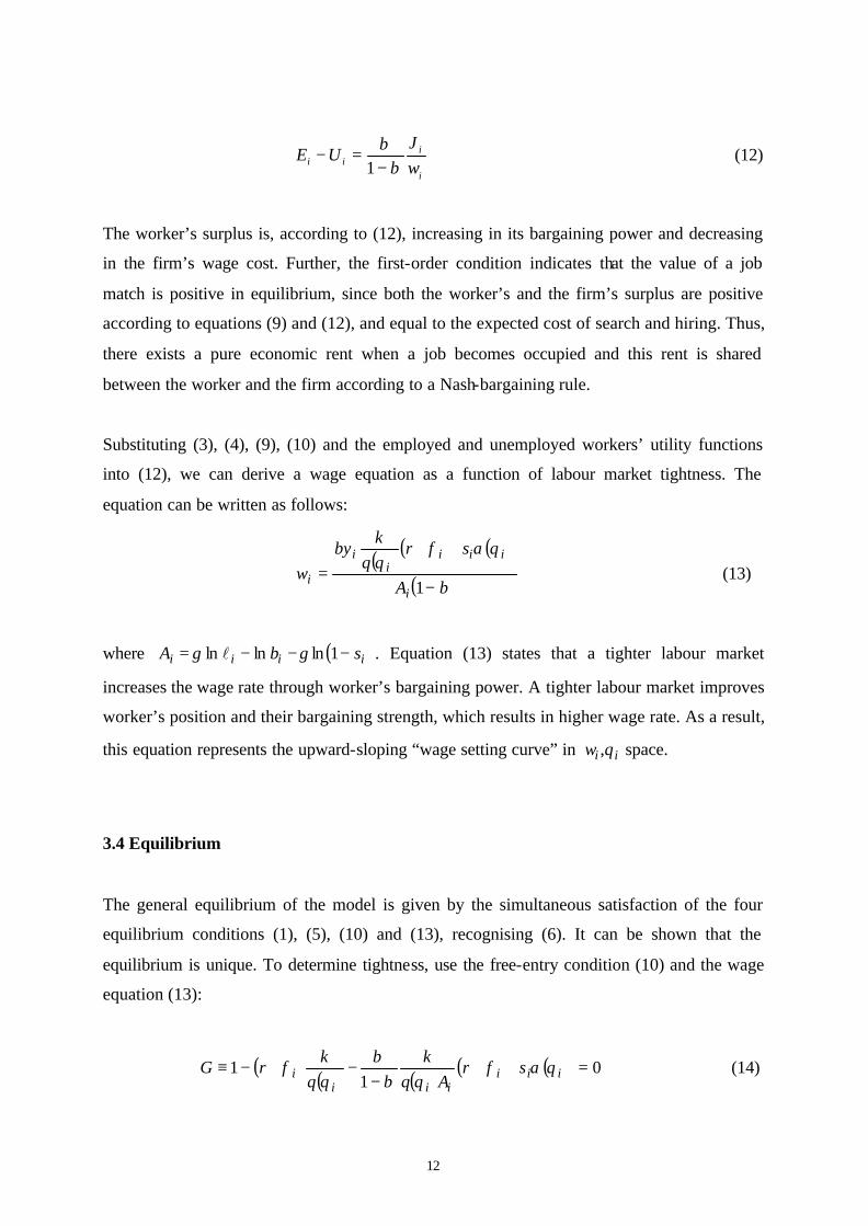
12

i

iii w

JUE

ββ−

=−1

(12)

The worker’s surplus is, according to (12), increasing in its bargaining power and decreasing

in the firm’s wage cost. Further, the first-order condition indicates that the value of a job

match is positive in equilibrium, since both the worker’s and the firm’s surplus are positive

according to equations (9) and (12), and equal to the expected cost of search and hiring. Thus,

there exists a pure economic rent when a job becomes occupied and this rent is shared

between the worker and the firm according to a Nash-bargaining rule.

Substituting (3), (4), (9), (10) and the employed and unemployed workers’ utility functions

into (12), we can derive a wage equation as a function of labour market tightness. The

equation can be written as follows:

( ) ( )( )

( )β

θαφθ

β

−

++=

1i

iiii

i

i A

srq

ky

w (13)

where ( )iiii sbA −−−= 1lnlnln γγ l . Equation (13) states that a tighter labour market

increases the wage rate through worker’s bargaining power. A tighter labour market improves

worker’s position and their bargaining strength, which results in higher wage rate. As a result,

this equation represents the upward-sloping “wage setting curve” in iiw θ, space.

3.4 Equilibrium

The general equilibrium of the model is given by the simultaneous satisfaction of the four

equilibrium conditions (1), (5), (10) and (13), recognising (6). It can be shown that the

equilibrium is unique. To determine tightness, use the free-entry condition (10) and the wage

equation (13):

( )( ) ( )

( )( ) 01

1 =++−

−+−≡ iiiiii

i srAq

kq

krG θαφ

θββ

θφ (14)

13

where 0=sG , a property implied by optimal search behaviour. Given tightness, equation (5)

determines search behaviour. With tightness and search determined, equation (1) gives

unemployment. Finally, taxes can be determined once wages and unemployment are

determined. The government’s budget constraint takes the form:

( )[ ] ( )[ ] 222111222222111111 11 wbuwbuwbuwuwbuwu +=+−++− ττ

Note that 12 yy > implies 12 ww > for 21 bb = and 21 φφ = . Equation (14) implies that

labour market tightness is independent of the tax rate and productivity in equilibrium. The

same result can be shown for search effort, i.e., a change in labour productivity or tax rate

does not affect search effort even though changes in productivity affect wages. It means also,

by using (1), that equilibrium unemployment is independent of the level of productivity and

the tax rate.

However, a higher replacement rate, ib , reduces labour market tightness through a higher

wage. To see this, differentiate (14) implicitly to get 0<i

Gθ and 0<ibG . A rise in the

worker’s bargaining power, β , has a similar effect for similar reasons. It is also obvious that

an increase in the separation rate, iφ , or a higher vacancy cost, k , decreases tightness.

4. The Optimal Structure of Replacement Rates

Consider a social welfare function of utilitarian form, that is

( )[ ]iiiii

rUurEuW +−= Σ 1

To compare different steady state without considering the adjustment process, let the discount

rate approach zero, i.e. 0→r , and substitute the value functions into the welfare function.

We get an expression for social welfare that is simplified to a weighted average of workers’

instantaneous utilities:

( )[ ]uii

eii

ii

ivuvuWW +−== ΣΣ 1

14

4.1 Paretoefficiency

Let us first examine a Pareto efficient UI policy by maximising the expected utility of agent 1,

given the expected utility of agent 2. Rewrite the utilitarian welfare function:

( ) ( ) ( ) iiiiiiiii HwbuwuW +−+−−≡ ττ 1ln1ln1

( ) iiiii Hbuw ++−+= ln1lnln τ (15)

where ( ) ( ) ( )iiii sTuhTuH −+−−≡ lnln1 γγ captures the leisure components. The budget

restriction is

( )[ ] 012,1

=−+−≡Ω Σ=

iiiiiiiii

wbuwbuuτ (16)

Let L denote the value of the Lagrangian and µ the Lagrange multiplier on the utility

constraint, and λ the Lagrange multiplier on the budget constraint. The Lagrangian for this

problem is

Ω+−+= λµ )( 21 RWWL (17)

where R is a given “promised” welfare for high-skilled workers. Differentiating with respect

to each of the choice variables gives us the first-order conditions:

011

1

1=

Ω+=

dbd

dbdW

dbdL

λ (18)

022

2

2=

Ω+=

dbd

dbdW

dbdL

λµ (19)

011

1

1=

Ω+=

τλ

ττ dd

ddW

ddL

(20)

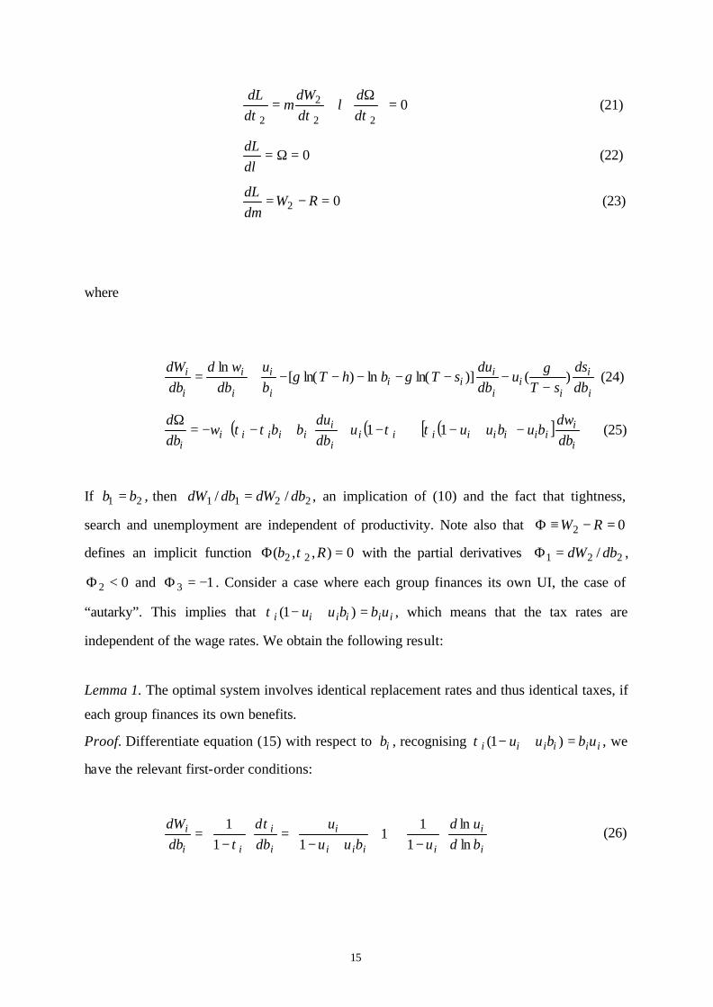
15

022

2

2=

Ω+=

τλ

τµ

τ dd

ddW

ddL

(21)

0=Ω=λd

dL (22)

02 =−= RWddLµ

(23)

where

i

i

ii

i

iii

i

i

i

i

i

i

dbds

sTu

dbdu

sTbhTbu

dbwd

dbdW

)()]ln(ln)ln([ln

−−−−−−−+=

γγγ (24)

( ) ( ) ( )[ ]i

iiiiiiiii

i

iiiiii

i dbdw

bubuuudbdu

bbwdbd

−+−+

−++−−=

Ω11 ττττ (25)

If 21 bb = , then 2211 // dbdWdbdW = , an implication of (10) and the fact that tightness,

search and unemployment are independent of productivity. Note also that 02 =−≡Φ RW

defines an implicit function 0),,( 22 =Φ Rb τ with the partial derivatives 221 / dbdW=Φ ,

02 <Φ and 13 −=Φ . Consider a case where each group finances its own UI, the case of

“autarky”. This implies that iiiiii ubbuu =+− )1(τ , which means that the tax rates are

independent of the wage rates. We obtain the following result:

Lemma 1. The optimal system involves identical replacement rates and thus identical taxes, if

each group finances its own benefits.

Proof. Differentiate equation (15) with respect to ib , recognising iiiiii ubbuu =+− )1(τ , we

have the relevant first-order conditions:

−

+

+−

=

−

=i

i

iiii

i

i

i

ii

i

bdud

ubuuu

dbd

dbdW

lnln

11

111

1 ττ

(26)

16

Equation (26) says that, in optimum, the welfare cost of increasing tax rates is equal to the

welfare gain from a rise in the replacement rate. The right hand side term in (26) captures the

welfare cost implied by the associated tax increase, whereas the left hand side term captures

the welfare gain from a rise in the replacement rate. Inspecting (26) and recognising (24)

implies that 21 bb = is optimal, since labour productivity does not enter the expression. Thus,

we have 21 ττ = since 21 uu = at 21 bb = . QED.

Let *iW denote the expected utility of a type i worker under autarky. Note that *

1*2 WW >

since high productivity workers enjoy higher consumption levels. We can establish the

following result:

Proposition 1. (i) For *2WR = , benefit differentiation is not optimal. (ii) For *

2WR < , benefit

differentiation, i.e., 21 bb > , is optimal provided that a benefit rise reduces the wage bill.

Proof. Note that 2211 // dbdWdbdW = at bbb == 21 and suppose that (18) holds and

consider the change in welfare arising from an increase in 2b :

=

Ω−

Ω=

= 12221

dbd

dbd

dbdL

bb

µλ

( ) ( ) 2222 1 wudbdu

bb

−++−− τττλ

( ) ( ) 1111 1 wudbdu

bb

−++−+ τττλµ

( )[ ]db

dwububu 2

2 1 −+−+ τλ

( )[ ]dbdw

ububu 11 1 −+−− τλµ (27)

It follows from (19), (20), (21) and uuu == 21 at bbb == 21 that ( )( ) 11

22

11

ww

ττ

µ−−

= . This

implies:

17

( )[ ]

−

−−

−=

= dbwud

uwdbdL

bb

1ln1

)1(1

122

221

τττ

λ (28)

where we have used the fact that dbwddbwddbwd /ln/ln/ln 21 == . From

0),,( 22 =Φ Rb τ we have 21 ττ ≤ as *2WR ≤ . Hence ( ) 0/

212 ==bbdbdL for *2WR = . For

*2WR < we have ( ) 0/

212 <=bbdbdL if ( )[ ] 0/1ln <− dbwud . QED.

The result in (i) that benefit differentiation is not Paretoimproving is not surprising. Suppose

an initial situation where the two groups are totally separate and each group finances its own

UI. This results to same replacement rate. Suppose now these two groups put together their

UI. Any distribution of replacement rate back and forth between the two groups make one

group better off and the other worse off. Thus, the allocation cannot be Pareto efficient.

Corollary 1. Benefit differentiation with 21 bb > is optimal if *2WR < and the labour demand

schedule is sufficiently wage inelastic. In particular, 0→σ is a sufficient condition for the

optimality of 21 bb > if *2WR < .

Proof. Define wuZ )1( −≡ and note that )/ln)(ln/ln(/ln dbddZddbZd θθ= , where

0/ln <dbd θ . Use the equilibrium conditions of the model to compute θln/ln dZd :20

−+

−+

+−

−

=wy

uwy

ss

ud

Zd1)1(1

1lnln

σσσθ

(29)

where 0ln/ln >θdZd , and thus 0/ln <dbZd , as 0→σ . QED. Equation (29) states that

there are two different mechanisms working in opposite directions. The bracketed expression

captures the employment effect whereas the last term captures the wage effect. An increase in

20 By using equations (1), (5), (10) and (13) we can write the wage bill as ))](,(1[)( θθθ suZ −= . The

function )(θs is obtained by combining the first-order condition for optimal search with the Nash bargaining

rule.

18

the replacement rate reduces employment but it also increases the wage rate so that total effect

on the tax base is generally ambiguous.

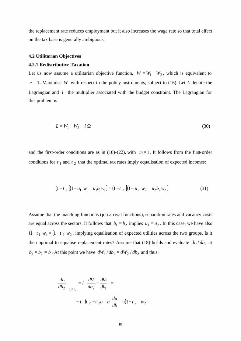
4.2 Utilitarian Objectives

4.2.1 Redistributive Taxation

Let us now assume a utilitarian objective function, 21 WWW +≡ , which is equivalent to

1=µ . Maximise W with respect to the policy instruments, subject to (16). Let L denote the

Lagrangian and λ the multiplier associated with the budget constraint. The Lagrangian for

this problem is

Ω++= λ21 WWL (30)

and the first-order conditions are as in (18)-(22), with 1=µ . It follows from the first-order

conditions for 1τ and 2τ that the optimal tax rates imply equalisation of expected incomes:

( ) ( )[ ] ( ) ( )[ ]222222111111 1111 wbuwuwbuwu +−−=+−− ττ (31)

Assume that the matching functions (job arrival functions), separation rates and vacancy costs

are equal across the sectors. It follows that 21 bb = implies 21 uu = . In this case, we have also

( ) ( ) 2211 11 ww ττ −=− , implying equalisation of expected utilities across the two groups. Is it

then optimal to equalise replacement rates? Assume that (18) ho lds and evaluate 2/ dbdL at

bbb == 21 . At this point we have 2211 // dbdWdbdW = and thus:

=

Ω−

Ω=

= 12221

dbd

dbd

dbdL

bb

λ

( ) ( ) 2222 1 wudbdu

bb

−++−− τττλ

19

( ) ( ) 1111 1 wudbdu

bb

−++−+ τττλ

( )[ ]db

dwububu 2

2 1 −+−+ τλ

( )[ ]db

dwububu 1

1 1 −+−− τλ (32)

Proposition 2. The optimal structure of replacement rates involves 12 bb < if wages are

exogenous.

Proof. Use the condition ( ) ( ) 2211 11 ww ττ −=− to substitute out 2τ from (32). The resulting

expression takes the form:

( ) ( )

−−−−=

= dbwd

udbdu

wwdbdL

bb

ln112

221

λ (33)

where we have used the fact tha t dbwddbwddbwd /ln/ln/ln 21 == . The second term in

the square bracket disappears with exogenous wages and thus we always have 0/ 2 <dbdL in

this case (so 21 bb = cannot be optimal). QED.

The sign is unclear in the general case. Note that expression (33) can also be written as

( )( ) ( )( )db

Zduww

dbwd

dbed

uwwdbdL

bb

ln1

lnln1 1212

221

−−=

+−−=

=

λλ (34)

where ue −= 1 is the employment rate and ewZ = is the wage bill. Equation (34) implies

that benefit differentiation is always optimal if labour demand elasticity is sufficiently low,

i.e., 0→σ .

20

4.2.2 Uniform Taxation

We have supposed so far that the government is free to choose separate tax rates for the two

categories, 1τ for group 1 (low skilled) and 2τ for group 2 (high skilled). Now, we will look

at a special case, i.e. we have a restriction on taxes: benefits are financed by a uniform

proportional tax rate, τ . The budget restriction is then

( ) ( )[ ] 011 2221112222211111 =+−+−++− wbuwbuwbuwuwbuwuτ (35)

To characterise the optimal UI policy in this case, the maximisation problem is:

( ) ( )[ ] ( ) ( )[ ] iiiiiii

ibbswbuwuW −+−++−−= ∑ 1ln1lnln1ln1max

,, 21

γτγττ

l

The Lagrangian for this problem is

( ) ( )[ ]222111222221111121 11 wubwubwbuwuwbuwuWWL −−+−++−++= ττττλ (36) Differentiating with respect to each of the choice variables gives us the first-order conditions:

( ) ( ) ( ) 011

1111111

1

1111

1

1

1=

+−−−+

−−+−−+=

dbdw

bubuuudbdu

bbwdbdW

dbdL

τττλτττλ (37)

( ) ( ) ( ) 012

2222222

2

2222

2

2

2=

+−−−+

−−+−−+=

dbdw

bubuuudbdu

bbwdbdW

dbdL

τττλτττλ

(38)

=τd

dL ( ) ( )[ ] 011 222221111121 =+−++−++ wbuwuwbuwu

ddW

ddW

λττ

(39)

=λd

dL ( ) ( )[ ]2221112222211111 11 wubwubwbuwuwbuwu −−+−++− ττττ 0= (40)

Should the two types have the same replacement rate or should one type have a higher benefit

level? Assume 21 φφ = , implying 12 ww > for 12 yy > . The following proposition

summarises the result:

21

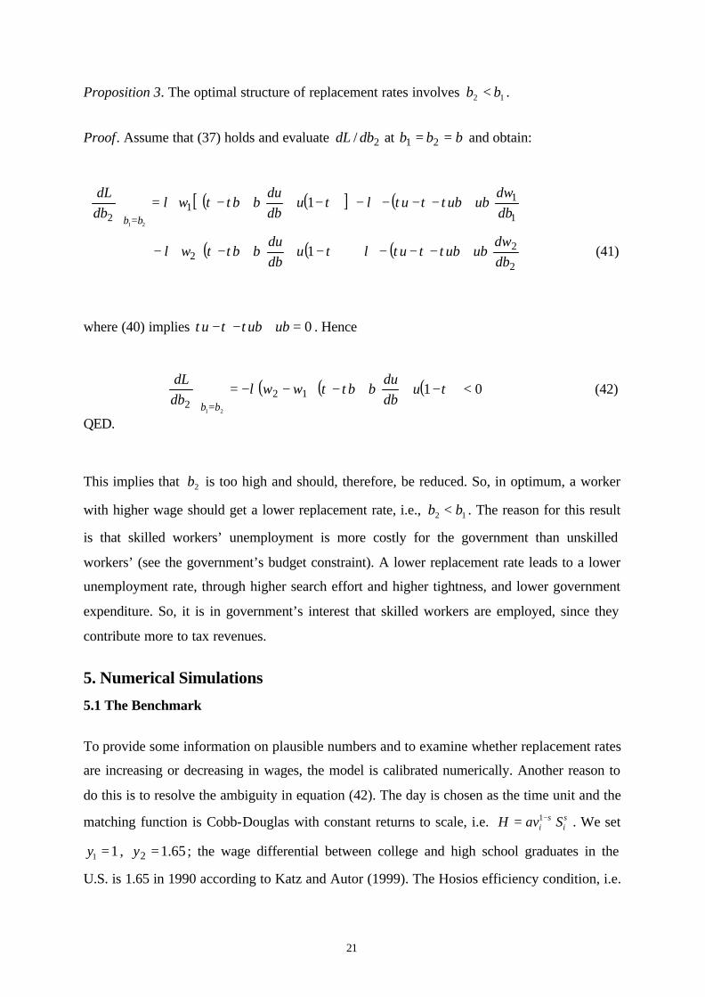
Proposition 3. The optimal structure of replacement rates involves 12 bb < .

Proof. Assume that (37) holds and evaluate 2/ dbdL at bbb == 21 and obtain:

[ ( ) ( ) ] ( )

+−−−−

−++−=

= 1

11

21

21dbdw

ububuudbdu

bbwdbdL

bb

τττλτττλ

( ) ( ) ( )

+−−−+

−++−−

2

22 1

dbdw

ububuudbdu

bbw τττλτττλ (41)

where (40) implies 0=+−− ububu τττ . Hence

( ) ( ) ( ) 01122

21

<

−++−−−=

=

τττλ udbdu

bbwwdbdL

bb

(42)

QED.

This implies that 2b is too high and should, therefore, be reduced. So, in optimum, a worker

with higher wage should get a lower replacement rate, i.e., 12 bb < . The reason for this result

is that skilled workers’ unemployment is more costly for the government than unskilled

workers’ (see the government’s budget constraint). A lower replacement rate leads to a lower

unemployment rate, through higher search effort and higher tightness, and lower government

expenditure. So, it is in government’s interest that skilled workers are employed, since they

contribute more to tax revenues.

5. Numerical Simulations

5.1 The Benchmark

To provide some information on plausible numbers and to examine whether replacement rates

are increasing or decreasing in wages, the model is calibrated numerically. Another reason to

do this is to resolve the ambiguity in equation (42). The day is chosen as the time unit and the

matching function is Cobb-Douglas with constant returns to scale, i.e. σσii SavH −= 1 . We set

11 =y , 65.12 =y ; the wage differential between college and high school graduates in the

U.S. is 1.65 in 1990 according to Katz and Autor (1999). The Hosios efficiency condition, i.e.

22

σβ = , is also imposed (see Hosios 1990). We set 5.0== σβ , which is a reasonable

approximation according to recent empirical studies of the matching function. 21

The real interest rate is equal to zero and the hours of work are set to )1/( γ+= Th , which is

what the employed worker would choose to maximise utility. The model is calibrated for a

uniform benefit system and 3.021 == bb , which is also close to the average replacement rates

in OECD countries according to Martin (1996). The remaining parameters are as follows:

023.0=a , 72.0=γ , 6.1=T , 13.4=k and 000828.021 == φφ , which implies an annual

separations rate of around 30% (see Layard et al 1991). The variables γ , 1φ , 2φ , T and k

were chosen such that we obtained 121 == ss and 065.021 == uu , which roughly matches

the recent average rate of unemployment in United States.22

Table 2 shows the results of the simulations.23 We have conducted two types of policy

experiments, the optimal uniform benefit system and the optimally differentiated benefit

system, and measure the welfare gain associated with particular policies. In all these

experiments there is always a decrease in replacement rates associated with an increase in

workers’ productivity. The last line of table 2 presents welfare gains associated with particular

policies. The welfare gain has the interpretation of a consumption tax that would make the

individual welfare across two policy regimes indifferent. The welfare ga ins are reported

relative to the base run that has a replacement rate of 30%. The welfare gain is measured by

the following equation

( )[ ] BP WcW =− ξ1

where BW represents welfare associated with the base run and PW is welfare associated with

an alternative policy. We let ξ denote the value of the tax rate that measures the welfare gain

of a particular policy relative to the base run.

21 See for example Broersma and Van Ours (1999) and Blanchard and Diamond (1989). 22See OECD (1997). 23 All simulations in this section concern redistributive taxation. For the uniform case see appendix.

23

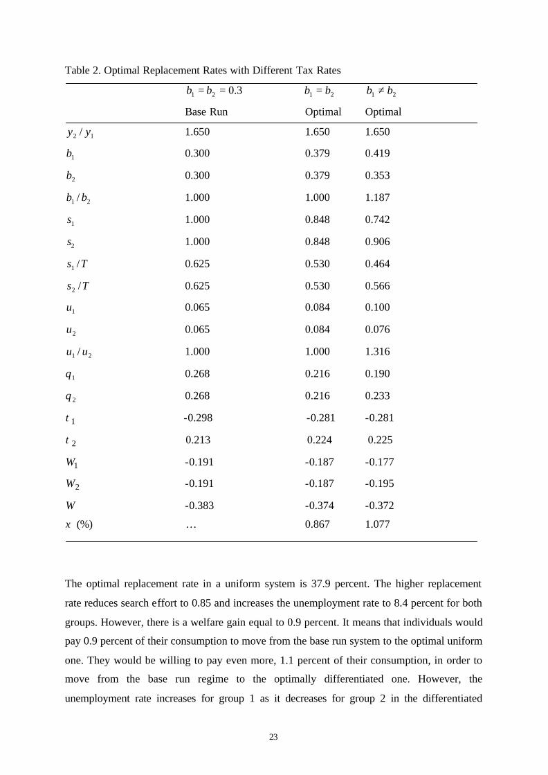
Table 2. Optimal Replacement Rates with Different Tax Rates

3.021 == bb 21 bb = 21 bb ≠

Base Run Optimal Optimal

12 / yy 1.650 1.650 1.650

1b 0.300 0.379 0.419

2b 0.300 0.379 0.353

21 / bb 1.000 1.000 1.187

1s 1.000 0.848 0.742

2s 1.000 0.848 0.906

Ts /1 0.625 0.530 0.464

Ts /2 0.625 0.530 0.566

1u 0.065 0.084 0.100

2u 0.065 0.084 0.076

21 / uu 1.000 1.000 1.316

1θ 0.268 0.216 0.190

2θ 0.268 0.216 0.233

1τ -0.298 -0.281 -0.281

2τ 0.213 0.224 0.225

1W -0.191 -0.187 -0.177

2W -0.191 -0.187 -0.195

W -0.383 -0.374 -0.372

ξ (%) … 0.867 1.077

The optimal replacement rate in a uniform system is 37.9 percent. The higher replacement

rate reduces search effort to 0.85 and increases the unemployment rate to 8.4 percent for both

groups. However, there is a welfare gain equal to 0.9 percent. It means that individuals would

pay 0.9 percent of their consumption to move from the base run system to the optimal uniform

one. They would be willing to pay even more, 1.1 percent of their consumption, in order to

move from the base run regime to the optimally differentiated one. However, the

unemployment rate increases for group 1 as it decreases for group 2 in the differentiated

24

regime compared with uniform regime which is not surprising since group 1’s replacement

rate rises but group 2’s declines.

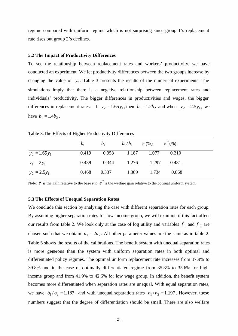
5.2 The Impact of Productivity Differences

To see the relationship between replacement rates and workers’ productivity, we have

conducted an experiment. We let productivity differences between the two groups increase by

changing the value of 2y . Table 3 presents the results of the numerical experiments. The

simulations imply that there is a negative rela tionship between replacement rates and

individuals’ productivity. The bigger differences in productivities and wages, the bigger

differences in replacement rates. If 12 65.1 yy = , then 21 2.1 bb = and when 12 5.2 yy = , we

have 21 4.1 bb = .

Table 3.The Effects of Higher Productivity Differences

1b 2b 21 / bb ε (%) *ε (%)

12 65.1 yy = 0.419 0.353 1.187 1.077 0.210

12 2yy = 0.439 0.344 1.276 1.297 0.431

12 5.2 yy = 0.468 0.337 1.389 1.734 0.868

Note: ε is the gain relative to the base run; *ε is the welfare gain relative to the optimal uniform system.

5.3 The Effects of Unequal Separation Rates

We conclude this section by analysing the case with different separation rates for each group.

By assuming higher separation rates for low-income group, we will examine if this fact affect

our results from table 2. We look only at the case of log utility and variables 1φ and 2φ are

chosen such that we obtain 21 2uu = . All other parameter values are the same as in table 2.

Table 5 shows the results of the calibrations. The benefit system with unequal separation rates

is more generous than the system with uniform separation rates in both optimal and

differentiated policy regimes. The optimal uniform replacement rate increases from 37.9% to

39.8% and in the case of optimally differentiated regime from 35.3% to 35.6% for high

income group and from 41.9% to 42.6% for low wage group. In addition, the benefit system

becomes more differentiated when separation rates are unequal. With equal separation rates,

we have 187.1/ 21 =bb , and with unequal separation rates 197.1/ 21 =bb . However, these

numbers suggest that the degree of differentiation should be small. There are also welfare

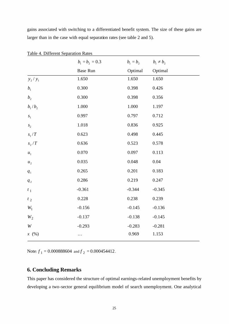
25

gains associated with switching to a differentiated benefit system. The size of these gains are

larger than in the case with equal separation rates (see table 2 and 5).

Table 4. Different Separation Rates

3.021 == bb 21 bb = 21 bb ≠

Base Run Optimal Optimal

12 / yy 1.650 1.650 1.650

1b 0.300 0.398 0.426

2b 0.300 0.398 0.356

21 / bb 1.000 1.000 1.197

1s 0.997 0.797 0.712

2s 1.018 0.836 0.925

Ts /1 0.623 0.498 0.445

Ts /2 0.636 0.523 0.578

1u 0.070 0.097 0.113

2u 0.035 0.048 0.04

1θ 0.265 0.201 0.183

2θ 0.286 0.219 0.247

1τ -0.361 -0.344 -0.345

2τ 0.228 0.238 0.239

1W -0.156 -0.145 -0.136

2W -0.137 -0.138 -0.145

W -0.293 -0.283 -0.281

ξ (%) … 0.969 1.153

Note: 000888604.01 =φ and 000454412.02 =φ .

6. Concluding Remarks

This paper has considered the structure of optimal earnings-related unemployment benefits by

developing a two-sector general equilibrium model of search unemployment. One analytical

26

result is that an optimal insurance system implies lower replacement rates for workers with

higher wages if taxes are uniform. The same result may hold even though taxes are

redistributive. The numerical results suggest that there are welfare gains associated with

switching from an optimal uniform benefit system to an optimally differentiated one in both

cases, i.e., uniform and redistributive taxation.

To gain insight into the essentials of the problem, saving has been ignored in the analysis.

Households can not smooth consumption through borrowing or private saving in the model.

Consumption is at the Polonius point.24 However, an analysis of equilibrium search including

saving would presumably make the model extremely complex.

A complete welfare analysis of UI policies should also take into account the fact that

unemployment benefits are often supplemented with family and housing benefits, which may

affect the behaviour of all individuals in the labour market. Another component to consider in

the analysis is the effects of eligibility rules on workers’ incentives. Existing UI system

require a number of conditions that the unemployed must satisfy in order to receive some

form of unemployment compensation, which means that many unemployed do not qualify for

benefits. A third factor we should keep in mind is the possibility that high wage ind ividuals

may have other incentives than the benefit level to search for a job when unemployed. These

factors may well have stronger effects on their search intensity and acceptance criteria than

unemployment benefits.

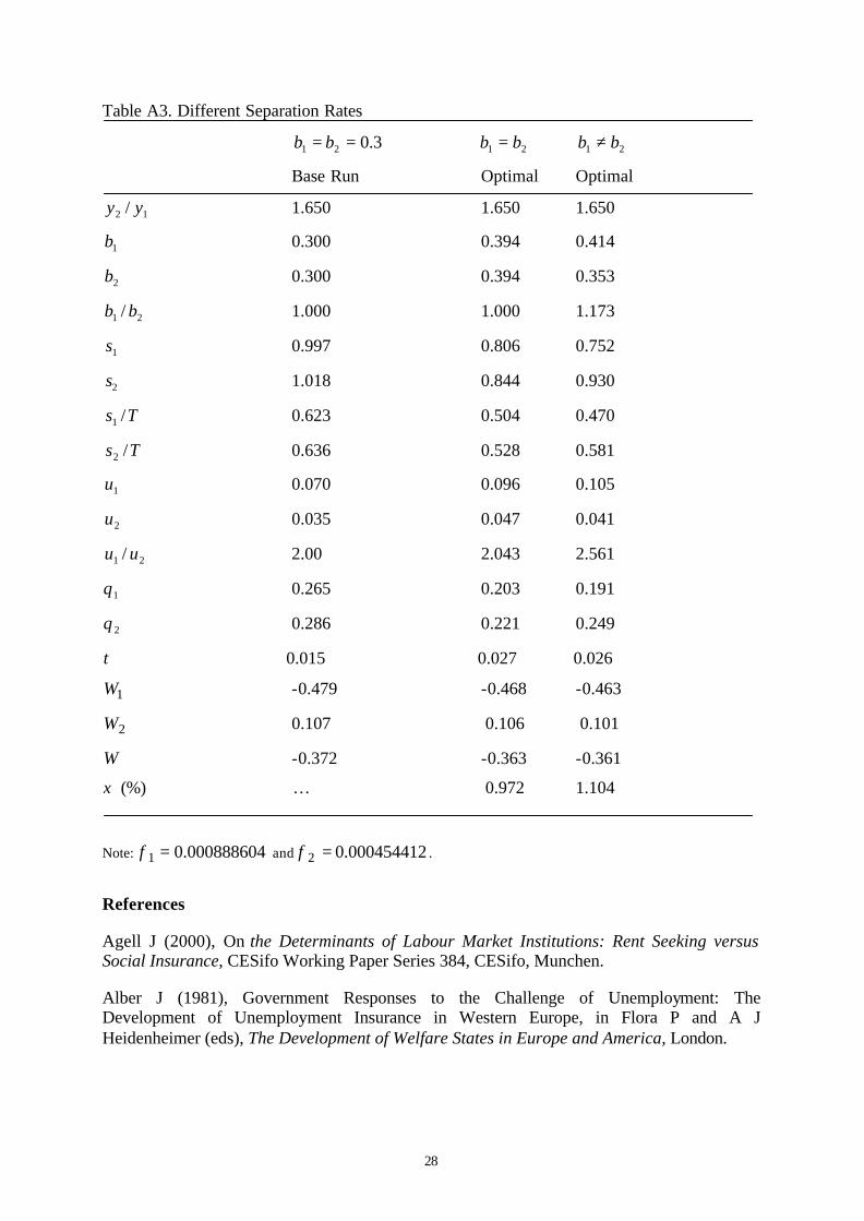
Appendix. Uniform Taxation

To see whether replacement rates and welfare gain changes when we move from an optimal

differentiated tax system to an optimal uniform tax system, we have also simulated the

uniform tax model. We use the same parameter values as in table 2. The effects on

replacement rates of switching from redistributive tax system to the uniform one seem to be

small and negligible (compare tables 2, 3 and 4 with A1, A2 and A3).

24 Hamlet, Act I, scene III; Polonius giving advice to his son, Leartes: “Neither a borrower nor a lender be: for loan oft loses both itself and friend; and borrowing dulls the edge of husbandry.” ( Shakespeare 1601). I owe this reference to Varian (1996).

27

Table A1. Optimal Replacement Rates

3.021 == bb 21 bb = 21 bb ≠

Base Run Optimal Optimal

12 / yy 1.650 1.650 1.650

1b 0.300 0.379 0.410

2b 0.300 0.379 0.350

21 / bb 1.000 1.000 1.171

1s 1.000 0.848 0.768

2s 1.000 0.848 0.910

Ts /1 0.625 0.530 0.480

Ts /2 0.625 0.530 0.569

1u 0.065 0.084 0.096

2u 0.065 0.084 0.075

21 / uu 1.000 1.000 1.280

1θ 0.268 0.216 0.195

2θ 0.268 0.216 0.234

τ 0.020 0.033 0.033

1W -0.473 -0.468 -0.461

2W 0.028 0.032 0.026

W -0.445 -0.436 -0.434

ξ (%) … 0.867 1.039

Table A2.The Effects of Higher Productivity Differences

1b 2b 21 / bb ε (%) *ε (%)

12 65.1 yy = 0.410 0.350 1.171 1.039 0.172

12 2yy = 0.422 0.341 1.238 1.190 0.323

12 5.2 yy = 0.434 0.330 1.315 1.443 0.542

Note: ε is the gain relative to the base run; *ε is the welfare gain relative to the optimal uniform system.

28

Table A3. Different Separation Rates

3.021 == bb 21 bb = 21 bb ≠

Base Run Optimal Optimal

12 / yy 1.650 1.650 1.650

1b 0.300 0.394 0.414

2b 0.300 0.394 0.353

21 / bb 1.000 1.000 1.173

1s 0.997 0.806 0.752

2s 1.018 0.844 0.930

Ts /1 0.623 0.504 0.470

Ts /2 0.636 0.528 0.581

1u 0.070 0.096 0.105

2u 0.035 0.047 0.041

21 / uu 2.00 2.043 2.561

1θ 0.265 0.203 0.191

2θ 0.286 0.221 0.249

τ 0.015 0.027 0.026

1W -0.479 -0.468 -0.463

2W 0.107 0.106 0.101

W -0.372 -0.363 -0.361

ξ (%) … 0.972 1.104

Note: 000888604.01 =φ and 000454412.02 =φ .

References Agell J (2000), On the Determinants of Labour Market Institutions: Rent Seeking versus Social Insurance, CESifo Working Paper Series 384, CESifo, Munchen. Alber J (1981), Government Responses to the Challenge of Unemployment: The Development of Unemployment Insurance in Western Europe, in Flora P and A J Heidenheimer (eds), The Development of Welfare States in Europe and America, London.

29

Alber J and P Flora (1981), Modernisation, Democratization and the Development of Welfare States in Western Europe, in Flora P and J Heidenheimer (eds), The Development of Welfare States in Europé and America, London. Atkinson A and J Micklewright (1991), Unemployment Compensation and Labour Market Transitions: A Critical Review, Journal of Economic Literature 29: 1979-1727. Baily M A (1978), Some Aspects of Optimal Unemployment Insurance, Journal of Public Economics 10: 379-402. Blanchard O J and P Diamond (1989), The Beveridge Curve, Brooking Papers on Economic Activity, no. 1: 1-60. Broersma L and J C Van Ours (1999), Job Searchers, Job Matches and the Elasticity of Matching, Labour Economics 6: 77-93. Brooks J (1893), Compulsory Insurance in Germany, Washington. Devine T and N Kiefer (1991), Empirical Labour Economics: The Search Approach, Oxford University Press. Esping-Andersen G (1990), The Three Worlds of Welfare Capitalism, Cambridge. Flemming J (1978), Aspects of Optimal Unemployment Insurance: Search, Leisure, Savings and Capital Market Imperfections, Journal of Public Economics 10:403-25. Flora P (1987), State, Economy and Society in Western Europe 1815-1975, London: Macmillan. Fredriksson P and B Holmlund (2001), Optimal Unemployment Insurance in Search Equilibrium, Journal of Labour Economics 19 (2): 370-399. Freeman R B (1998), War of the Models: Which Labour Market Institutions for the 21st Century?, Labour Economics 5: 1-24. Holmlund B (1998), Unemployment Insurance in Theory and Practice, Scandinavian Journal of Economics 100 (1): 113-141. Hosios A (1990), On the Efficiency of Matching and Related Models of Search and Unemployment, Review of Economic Studies 57: 279-98. Johnson G and R Layard (1986), The Natural Rate of Unemployment: Explanation and Policy, in O Ashenfelter and R Layard (eds), Handbook of Labour Economics, vol. 1, North Holland. Katz L F and D H Autor (1999), Changes in the Wage Structure and Earnings Inequality, in O Ashenfelter and D Card (eds), Handbook of Labour Economics, vol. 3A, North Holland. Layard R, S Nickell and R Jackman (1991), Unemployment: Macroeconomic Performance and the Labour Market, Oxford.

30

Leibfried S (1993), Towards a European Welfare State? in Jones C (ed), New Perspective on the Welfare State in Europe, London Leman C (1980), The Collapse of Welfare Reform: Political Institutions, Policy, and the Poor in Canada and the United States, MIT Press, Cambridge. Martin J (1996), Measures of Replacement Rates for the Purpose of International Comparisons: A Note, OECD Economic Studies 26: 99-115. Mortensen D (1977), Unemployment Insurance and Job Search Decisions, Industrial and Labor Relations Review 30 (4):505-17. Munzi T and A Salomäki (1999), Net Replacement Rates of the Unemployed. Comparisons of Various Approches, OECD Economic Papers, OECD. Organisation for Economic Co-Operation and Development, OECD (1999), Benefit System and Work Incentives, Paris. Petrongolo B and C Pissarides (2001), Looking into the Black Box: a Survey of the Matching Function, Journal of Economic Litterature 39: 390-431. Pissarides C A (2000), Equilibrium Unemployment Theory, Basil Blackwell, MIT Press. Shakespeare W (1601), Hamlet, England. Shavell S and L Weiss (1979), The Optimal Payment of Unemployment Insurance Benefits over Time, Journal of Political Economy 87: 1347-62. SOU (1996), Grundläggande drag i en ny arbetslöshetsförsäkring (The Main Features of a New Unemployment Insurance), SOU 1996:51, Stockholm. Tsukada H (2002), Economic Globalization and the Citizens’ Welfare State, England. Varian H (1996), Intermediate Microeconomics : A Modern Approach, New York.