Hour to hour syllabus for Math21b, Fall 2010

Course Head: Oliver Knill

Abstract

Here is a brief outline of the lectures for the fall 2010 semester. The section numbers refer to the book

of Otto Bretscher, Linear algebra with applications.

1. Week: Systems of Linear Equations and Gauss-Jordan

1. Lecture: Introduction to linear systems, Section 1.1, September 8, 2010

A central point of this week is Gauss-Jordan elimination. While the precise procedure will be introduced inthe second lecture, we learn in this first hour what a system of linear equations is by looking at examplesof systems of linear equations. The aim is to illustrate, where such systems can occur and how one could solvethem with ’ad hoc’ methods. This involves solving equations by combining equations in a clever way or toeliminate variables until only one variable is left. We see examples with no solution, several solutions or exactlyone solution.

2. Lecture: Gauss-Jordan elimination, Section 1.2, September 10,2010

We rewrite systems of linear equations using matrices and introduce Gauss-Jordan elimination steps:scaling of rows, swapping rows or subtract a multiple of one row to an other row. We also see an example,where one has not only one solution or no solution. Unlike in multi-variable calculus, we distinguish betweencolumn vectors and row vectors. Column vectors are n× 1 matrices, and row vectors are 1×m matrices. Ageneral n×m matrix has m columns and n rows. The output of Gauss-Jordan elimination is a matrix rref(A)which is in row reduced echelon form: the first nonzero entry in each row is 1, called leading 1, every columnwith a leading 1 has no other nonzero elements and every row above a row with a leading 1 has a leading 1 tothe left.

2. Week: Linear Transformations and Geometry

3. Lecture: On solutions of linear systems, Section 1.3, September 13,2010

How many solutions does a system of linear equations have? The goal of this lecture is to see that there arethree possibilities: exactly one solution, no solution or infinitely many solutions. This can be visualized andexplained geometrically in low dimensions. We also learn to determine which case we are in using Gauss-Jordanelimination by looking at the rank of the matrix A as well as the augmented matrix [A|b]. We also mentionthat one can see a system of linear equations Ax = b in two different ways: the column picture tells thatb = x1v1+ · · ·+xnvn is a sum of column vectors vi of the matrix A, the row picture tells that the dot productof the row vectors wj with x are the components wj · x = bj of b.

4. Lecture: Linear transformation, Section 2.1, September 15,2010

1

This week provides a link between the geometric and algebraic description of linear transformations. Lineartransformations are introduced formally as transformations T (x) = Ax, where A is a matrix. We learn how todistinguish between linear and nonlinear, linear and affine transformations. The transformation T (x) = x + 5for example is not linear because 0 is not mapped to 0. We characterize linear transformations on Rn by threeproperties: T (0) = 0, T (x+ y) = T (x)+T (y) and T (sx) = sT (x), which means compatibility with the additivestructure on Rn.

5. Lecture: Linear transformations in geometry, Section 2.2, September 17,2010

We look at examples of rotations, dilations, projections, reflections, rotation-dilations or shears. How are thesetransformations described algebraically? The main point is to see how to go forth and back between algebraicand geometric description. The key fact is that the column vectors vj of a matrix are the images vj = Tej ofthe basis vectors ej. We derive for each of the mentioned geometric transformations the matrix form. Any ofthem will be important throughout the course.

3. Week: Matrix Algebra and Linear Subspaces

6. Lecture: Matrix product, Section 2.3, September 20, 2010

The composition of linear transformations leads to the product of matrices. The inverse of a transformationis described by the inverse of the matrix. Square matrices can be treated in a similar way as numbers: wecan add them, multiply them with scalars and many matrices have inverses. There is two things to be carefulabout: the product of two matrices is not commutative and many nonzero matrices have no inverse. If we takethe product of a n × p matrix with a p ×m matrix, we obtain a n ×m matrix. The dot product as a specialcase of a matrix product between a 1× n matrix and a n× 1 matrix. It produces a 1× 1 matrix, a scalar.

7. Lecture: The inverse, Section 2.4, September 22, 2010

We first look at invertibility of maps f : X → X in general and then focus on the case of linear maps. If alinear map Rn to Rn is invertible, how do we find the inverse? We look at examples when this is the case.Finding x such that Ax = y is equivalent to solving a system of linear equations. Doing this in parallel gives usan elegant algorithm by row reducing the matrix [A|1n] to end up with [1n|A−1]. We also might have time to

see how upper triangular block matrices

[

A B0 C

]

have the inverse

[

A−1 −A−1BC−1

0 C−1

]

.

8. Lecture: Image and kernel, Section 3.1, September 24, 2010

We define the notion of a linear subspace of n-dimensional space and the span of a set of vectors. Thisis a preparation for the more abstract definition of linear spaces which appear later in the course. The mainalgorithm is the computation of the kernel and the image of a linear transformation using row reduction. Theimage of a matrix A is spanned by the columns of A which have a leading 1 in rref(A). The kernel of a matrixA is parametrized by ”free variables”, the variables for which there is no leading 1 in rref(A). For a n × nmatrix, the kernel is trivial if and only if the matrix is invertible. The kernel is always nontrivial if the n×mmatrix satisfies m > n, that is if there are more variables than equations.

4. Week: Basis and Dimension

9. Lecture: Basis and linear independence, Section 3.2, September 27, 2010

2

With the previously defined ”span” and the newly introduced linear independence, one can define what a basis

for a linear space is. It is a set of vectors which span the space and which are linear independent. The standardbasis in Rn is an example of a basis. We show that if we have a basis, then every vector can be uniquely

represented as a linear combination of basis elements. A typical task is to find the basis of the kernel and thebasis for the image of a linear transformation.

10. Lecture: Dimension, Section 3.3, September 29, 2010

The concept of abstract linear spaces allows to introduce linear spaces of functions. This will be usefulfor applications in differential equations. We show first that the number of basis elements is independent ofthe basis. This number is called the dimension. The proof uses that if p vectors are linearly independentand q vectors span a linear subspace V , then p is less or equal to q. We see the rank-nullety theorem:dimker(A) + dimim(A) is the number of columns of A. Even so the result is not very deep, it is sometimesreferred to as the fundamental theorem of linear algebra. It will turn out to be quite useful for us, forexample, when looking under the hood of data fitting.

11. Lecture: Change of coordinates, Section 3.4, October 1, 2010

Switching to a different basis can be useful for certain problems. For example to find the matrix of the reflectionat a line or projection onto a plane, one can first find the matrix B in a suitable basis B = {v1, v2, v3 }, then useB = SAS−1 to get A. The matrix S contains the basis vectors in the columns. We also learn how to express amatrix in a new basis Sei = vi. We derive the formula B = SAS−1.

5. Week: Linear Spaces and Orthogonality

12. Lecture: Linear spaces, Section 4.1, October 4, 2010

In this lecture we generalize the concept of linear subspaces of Rn and consider abstract linear spaces. Anabstract linear space is a set X closed under addition and scalar multiplication and which contains 0. We lookat many examples. An important one is the space X = C([a, b]) of continuous functions on the interval [a, b] orthe space P5 of polynomials of degree smaller or equal to 5, or the linear space of all 3× 3 matrices.

13. Lecture: Review for the second midterm, October 6, 2010

This is review for the first midterm on October 7th. The plenary review will cover all the material, so that thisreview can focus on questions or looking at some True/False problems or practice exam problems.

14. Lecture: orthonormal bases and projections, Section 5.1, October 8, 2010

We review orthogonality between vectors u,v by u · v = 0 and define orthonormal basis, a basis whichconsists of unit vectors which are all orthogonal to each other. The orthogonal complement of a linear spaceV in Rn is defined the set of all vectors perpendicular to all vectors in V . It can be found as a kernel ofthe matrix which contains a basis of V as rows. We then define orthogonal projection onto a linear subspaceV . Given an orthonormal basis {u1, . . . , un } in V , we have a formula for the orthogonal projection: P (x) =(u1 ·x)u1+ . . .+(un ·x)un. This simple formula for a projection only holds if we are given an orthonormal basisin the subspace V . We mention already that this formula can be written as P = AAT where A is the matrixwhich contains the orthonormal basis as columns.

6. Week: Gram-Schmidt and Projection

3

Monday is Columbus Day and no lectures take place.

15. Lecture: Gram-Schmidt and QR factorization, Section 5.2, October 13, 2010

The Gram Schmidt orthogonalization process lead to the QR factorization of a matrix A. We will look atthis process geometrically as well as algebraically. The geometric process of ”straightening out” and ”adjustinglength” can be illustrated well in 2 and 3 dimensions. Once the formulas for the orthonormal vectors wj froma given set of vectors vj are derived, one can rewrite it in matrix form. If the vj are the m columns of a n×mmatrix A and wj the columns of a n×m matrix Q, then A = QR, where R is a m×m matrix. This is the QRfactorization. The QR factorization has its use in numerical methods.

16. Lecture: Orthogonal transformations, Section 5.3, October 15, 2010

We first define the transpose AT of a matrix A. Orthogonal matrices are defined as matrices for whichATA = 1n. This is equivalent to the fact that the transformation T defined by A preserves angles and lengths.Rotations and reflections are examples of orthogonal transformations. We point out the difference betweenorthogonal projections and orthogonal transformations. The identity matrix is the only orthogonal matrixwhich is also an orthogonal projection. We also stress that the notion of orthogonal matrix only applies ton× n matrices and that the column vectors form an orthonormal basis. A matrix A for which all columns areorthonormal is not orthogonal if the number or rows is not equal to the number of columns.

7. Week: Data fitting and Determinants

17. Lecture: Least squares and data fitting, Section 5.4, October 18, 2010

This is an important lecture from the application point of view. It covers a part of statistics. We learn howto fit data points with any finite set of functions. To do so, we write the fitting problem as a in generaloverdetermined system of linear equations Ax = b and find from this the least square solution x∗ whichhas geometrically the property that Ax∗ is the projection of b onto the image of A. Because this meansAT (Ax∗ − b) = 0, we get the formula

x∗ = (ATA)−1Ab .

An example is to fit a set of data (xi, yi) by linear functions {f1, ....fn}. This is very powerful. We can fit byany type of functions, even functions of several variables.

18. Lecture: Determinants I, Section 6.1, October 20, 2010

We define the determinant of a n×n matrix using the permutation definition. This immediately implies theLaplace expansion formula and allows comfortably to derive all the properties of determinants from the originaldefinition. In this lecture students learn about permutations in terms of patterns. There is no need to talkabout permutations and signatures. The equivalent language of ”patterns” and ”number of ”upcrossings”.In this lecture, we see the definition of determinants in all dimensions, see how it fits with 2 and 3 dimensionalcase. We practice already Laplace expansion to compute determinants.

19. Lecture: Determinants II, Section 6.2, October 22, 2010

We learn about the linearity property of determinants and how Gauss-Jordan elimination allows a fastcomputation of determinants. The computation of determinants by Gauss-Jordan elimination is quite efficient.Often we can see the determinant already after a few steps because the matrix has become upper triangular.We also point out how to compute determinants for partitioned matrices. We do lots of examples, also harderexamples in which we learn how to decide which of the methods to use: permutation method, Laplace expansion,row reduction to a triangular case or using partitioned matrices.

4

8. Week: Eigenvectors and Diagonalization

20. Lecture: Eigenvalues, Section 7.1-2, October 25, 2010

Eigenvalues and eigenvectors are introduced in this lecture. It is good to see them first in concrete exampleslike rotations, reflections, shears. As the book, we can motivate the concept using discrete dynamical

systems, like the problem to find the growth rate of the Fibonacci sequence. Here it becomes evident, whycomputing eigenvalues and eigenvectors is useful.

21. Lecture: Eigenvectors, Section 7.3, October 27, 2010

This lecture focuses on eigenvectors. Computing eigenvectors relates to the computation of the kernel of a lineartransformation. We give also a geometric idea what eigenvectors are and look at lots of examples. A good classof examples are Markov matrices, which are important from the application point of view. Markov matricesalways have an eigenvalue 1 because the transpose has an eigenvector [1, 1, . . .1]T . The eigenvector of A to theeigenvalue 1 has significance. It belongs to a stationary probability distribution.

22. Lecture: Diagonalization, Section 7.4, October 29, 2010

A major result of this section is that if all eigenvalues of a matrix are different, one can diagonalize the matrixA. There is an eigenbasis. We also see that if the eigenvalues are the same, like for the shear matrix, one cannot diagonalize A. If the eigenvalues are complex like for a rotation, one can not diagonalize over the reals.Since we like to able to diagonalize in as many situations as possible, we allow complex eigenvalues from nowon.

9. Week: Stability of Systems and Symmetric Matrices

23. Lecture: Complex eigenvalues, Section 7.5, November 1, 2010

We start with a short review on complex numbers. Course assistants will do more to get the class up to speedwith complex numbers. The fundamental theorem of algebra assures that a polynomial of degree n hasn solutions, when counted with multiplicities. We express the determinant and trace of a matrix in terms ofeigenvalues. Unlike in the real case, these formulas hold for any matrix.

24. Lecture: Review for second midterm, November 3, 2010

We review for the second midterm in section. Since there was a plenary review for all students covering thetheory, one could focus on student questions and see the big picture or discuss some True/False problems orpractice exam problems.

25. Lecture: Stability, Section 7.6, November 5, 2010

We study the stability problem for discrete dynamical systems. The absolute value of the eigenvalues deter-mines the stability of the transformation. If all eigenvalues are in absolute value smaller than 1, then the originis asymptotically stable. A good example to discuss is the case, when the matrix is not diagonalizable, like

for example for a shear dilation S =

[

0.99 10000 0.99

]

, where the expansion by the off diagonal shear competes

with the contraction in the diagonal.

5

10. Week: Homogeneous Ordinary Differential Equations

26. Lecture: Symmetric matrices, Section 8.1, November 8, 2010

The main point of this lecture is to see that symmetric matrices can be diagonalized. The key fact is that theeigenvectors of a symmetric matrix are perpendicular to each other. An intuitive proof of the spectral theoremcan be given in class: after a small perturbation of the matrix all eigenvalues are different and diagonalizationis possible. When making the perturbation smaller and smaller, the eigenspaces stay perpendicular and inparticular linearly independent. The shear is the prototype of a matrix, which can not be diagonalized. Thislecture also gives plenty of opportunity to practice finding an eigenbasis and possibly for Gramm-Schmidt, ifan orthonormal eigenbasis needs to be found in a higher dimensional eignspace.

27. Lecture: Differential equations I, Section 9.1, November 10, 2010

We learn to solve systems of linear differential equations by diagonalization. We discuss linear stabilityof the origin. Unlike in the discrete time case, where the absolute value of the eigenvalues mattered, the realpart of the eigenvalues is now important. We also keep in mind the one dimensional case, where these facts areobvious. The point is that linear algebra allows to reduce the higher dimensional case to the one-dimensionalcase.

28. Lecture: Differential equations II, Section 9.2, November 12, 2010

A second lecture is necessary for the important topic of applying linear algebra to solve differential equations

x′ = Ax, where A is a n × n matrix. While the central idea is to diagonalize A and solve y′ = By, where Bis diagonal, we can do so a bit faster. Write the initial condition x(0) as a linear combination of eigenvectorsx(0) = a1v1+. . .+anvn and get x(t) = a1v1e

λ1t+. . .+anvneλnt. We also look at examples where the eigenvalues

λ1 of the matrix A are complex. An important case for the later is the harmonic oscillator with and withoutdamping. There would be many more interesting examples from physics.

11. Week: Nonlinear Differential Equations, Function spaces

29. Lecture: Nonlinear systems, Section 9.4, November 15, 2010

This section is covered by a separate handout numbered Section 9.4. How can nonlinear differential equa-

tions in two dimensions x = f(x, y), y = g(x, y) be analyzed using linear algebra? The key concepts are findingnull clines, equilibria and their nature using linearization of the system near the equilibria by comput-ing the Jacobean matrix. Good examples are competing species systems like the example of Murray,predator-pray examples like the Volterra system or mechanical systems like the pendulum.

30. Lecture: Linear operators, Section 4.2, November 17, 2010

We study linear operators on linear spaces. The main example is the operator Df = f ′ as well as polynomialsof the operator D like D2 + D + 1. Other examples T (f) = xf, T (f)(x) = x + 3 (which is not linear) orT (f)(x) = x2f(x) which is linear. The goal is of this lecture is to get ready to understand that solutions ofdifferential equations are kernels of linear operators or write partial differential equations in the form ut = T (u),where T is a linear operator.

31. Lecture: Linear differential operators, Section 9.3, November 19, 2010

6

The main goal is to be able to solve linear higher order differential equations p(D) = g using the operator

method. The method generalizes the integration process which we use to solve for examples like f ′′′ = sin(x)where three fold integration leads to the general solution f . For a problem p(D) = g we factor the polynomialp(D) = (D− a1)(D− a2)...(D− an) into linear parts and invert each linear factor (D− ai) using an integrationfactor. This operator method is very general and always works. It also provides us with a justification for amore convenient way to find solutions.

12. Week: Inner product Spaces and Fourier Theory

32. Lecture: inhomogeneous differential equations, Handout, November 22, 2010

This operator method to solve differential equations p(D)f = g works unconditionally. It allows to put togethera ”cookbook method”, which describes, how to find the special solution of the inhomogeneous problem by firstfinding the general solution to the homogeneous equation and then finding a special solution. Very importantcases are the situation x− ax = g(x), the driven harmonic oscillator

x+ c2x = g(x)

or the driven damped harmonic oscillator

x+ bx+ c2x = g(x)

Special care has to be taken if g(x) is in the kernel of p(D) or if the polynomial p has repeated roots.

33. Lecture: Inner product spaces, Section 5.5, November 24, 2010

As a preparation for Fourier theory we introduce inner products in linear spaces. It generalizes the dotproduct. For 2π-periodic functions, one takes 〈f, g〉 as the integral of f g from −π to π and divide by 2π. It hasall the properties we know from the dot product in finite dimensions. An other example of an inner producton matrices is 〈A,B〉 = tr(ATB). Most of the geometry we did before can now be done in a larger context.Examples are Gram-Schmidt orthogonalization, projections, reflections, have the concept of coordinates in abasis, orthogonal transformations etc.

13. Week: Fourier Series and Partial differential equations

34. Lecture: Fourier series, Handout, November 29, 2010

The expansion of a function with respect to the orthonormal basis 1/√2, cos(nx), sin(nx) leads to the Fourier

expansion

f(x) = a0(1/√2) +

∞∑

n=1

an cos(nx) + bn sin(nx) .

A nice example to see how Fourier theory is useful is to derive the Leibniz series for π/4 by writing

x =

∞∑

k=1

2(−1)k+1

ksin(kx)

and evaluate it at π/2. The main motivation is that the Fourier basis is an orthonormal eigenbasis to theoperator D2. It diagonalizes this operator because D2 sin(nx) = −n2 sin(nx), D2 cos(nx) = −n2 cos(nx). Wewill use this to solve partial differential equations in the same way as we solved ordinary differential equations.

7

35. Lecture: Parseval’s identity, Handout, December 1, 2010

Parseval’s identity

||f ||2 = a20 +

∞∑

n=1

a2n + b2n .

is the ”Pythagorean theorem” for function spaces. It is useful to estimate how fast a finite sum converges.We mention also applications like computations of series by the Parseval’s identity or by relating them to aFourier series. Nice examples are computations of ζ(2) or ζ(4) using the Parseval’s identity.

36. Lecture: Partial differential equations, Handout, December 3, 2010

Linear partial differential equations ut = p(D)u or utt = p(D)u with a polynomial p are solved in thesame way as ordinary differential equations: by diagonalization. Fourier theory achieves that the ”matrix” D isdiagonalized and so the polynomial p(D). This is much more powerful than the separation of variable method,which we do not do in this course. For example, the partial differential equation

utt = uxx − uxxxx + 10u

can be solved nicely with Fourier in the same way as we solve the wave equation. The method allows even tosolve partial differential equations with a driving force like for example

utt = uxx − u+ sin(t) .

8

USE OF LINEAR ALGEBRA I Math 21b 2003-2010, O. Knill

1 2 3

4

GRAPHS, NETWORKS

Linear algebra can be used tounderstand networks. A networkis a collection of nodes connected byedges and are also called graphs.The adjacency matrix of a graphis an array of numbers defined byAij = 1 if there is an edge fromnode i to node j in the graph.Otherwise the entry is zero. Anexample of such a matrix appearedon an MIT blackboard in the movie”Good will hunting”.

How does the array of numbers helpto understand the network? Assumewe want to find the number of walksof length n in the graph which starta a vertex i and end at the vertex j.It is given by An

ij , where An is then-th power of the matrix A. Youwill learn to compute with matricesas with numbers. An other applica-tion is the ”page rank”. The net-work structure of the web allows toassign a ”relevance value” to eachpage, which corresponds to a prob-ability to hit the website.

CHEMISTRY, MECHANICS

Complicated objects like the Za-kim Bunker Hill bridge in Boston,or a molecule like a protein can bemodeled by finitely many parts.The bridge elements or atomsare coupled with attractive andrepelling forces. The vibrationsof the system are described by adifferential equation x = Ax, wherex(t) is a vector which depends ontime. Differential equations are animportant part of this course. Muchof the theory developed to solvelinear systems of equations can beused to solve differential equations.

The solution x(t) = exp(At)x(0) ofthe differential equation x = Axcan be understood and computed byfinding so called eigenvalues of thematrix A. Knowing these frequen-cies is important for the design ofa mechanical object because the en-gineer can identify and damp dan-gerous frequencies. In chemistry ormedicine, the knowledge of the vi-bration resonances allows to deter-mine the shape of a molecule.

QUANTUM COMPUTING

A quantum computer is a quan-tum mechanical system which isused to perform computations. Thestate x of a machine is no more asequence of bits like in a classicalcomputer, but a sequence of qubits,where each qubit is a vector. Thememory of the computer is a list ofsuch qbits. Each computation stepis a multiplication x 7→ Ax with asuitable matrix A.

Theoretically, quantum computa-tions could speed up conventionalcomputations significantly. Theycould be used for example for cryp-tological purposes. Freely availablequantum computer language (QCL)interpreters can simulate quantumcomputers with an arbitrary numberof qubits. Whether it is possible tobuild quantum computers with hun-dreds or even thousands of qubits isnot known.

CHAOS THEORY Dynami-

cal systems theory deals with theiteration of maps or the analysisof solutions of differential equations.At each time t, one has a map T (t)on a linear space like the plane. Thelinear approximationDT (t) is calledthe Jacobean. It is a matrix. Ifthe largest eigenvalue of DT (t) of Tgrows exponentially fast in t, thenthe system is called ”chaotic”.

Examples of dynamical systems area collection of stars in a galaxy,electrons in a plasma or particlesin a fluid. The theoretical studyis intrinsically linked to linear al-gebra, because stability propertiesoften depend on linear approxima-tions.

USE OF LINEAR ALGEBRA II Math 21b, O. Knill

CODING THEORY Coding

theory is used for encryption or er-ror correction. For encryption, datavectors x are mapped into the code

y = Tx. T usually is chosen to bea ”trapdoor function”: it is hard torecover x when y is known. For er-ror correction, a code can be a linearsubspace X of a vector space and Tis a map describing the transmissionwith errors. The projection onto Xcorrects the error.

Linear algebra enters in differentways, often directly because the ob-jects are vectors but also indirectlylike for example in algorithms whichaim at cracking encryption schemes.

DATA COMPRESSION Im-age, video and sound compression

algorithms make use of linear trans-formations like the Fourier trans-form. In all cases, the compres-sion makes use of the fact that inthe Fourier space, information canbe cut away without disturbing themain information.

Typically, a picture, a sound ora movie is cut into smaller junks.These parts are represented as vec-tors. If U is the Fourier transformand P is a cutoff function, theny = PUx is transferred or storedon a CD or DVD. The receiver likethe DVD player or the ipod recoversUT y which is close to x in the sensethat the human eye or ear does notnotice a big difference.

SOLVING EQUATIONS

When extremizing a functionf on data which satisfy a con-straint g(x) = 0, the method ofLagrange multipliers asks to solvea nonlinear system of equations∇f(x) = λ∇g(x), g(x) = 0 for the(n + 1) unknowns (x, l), where ∇fis the gradient of f .

Solving systems of nonlinear equa-tions can be tricky. Already for sys-tems of polynomial equations, onehas to work with linear spaces ofpolynomials. Even if the Lagrangesystem is a linear system, the solu-tion can be obtained efficiently usinga solid foundation of linear algebra.

GAMES Moving around in athree dimensional world like in acomputer game requires rotationsand translations to be implementedefficiently. Hardware accelerationcan help to handle this. We live in atime where graphics processor powergrows at a tremendous speed.

Rotations are represented by matri-ces which are called orthogonal.For example, if an object located at(0, 0, 0), turning around the y-axesby an angle φ, every point in the ob-ject gets transformed by the matrix

cos(φ) 0 sin(φ)0 1 0

− sin(φ) 0 cos(φ)

CRYPTOLOGY Much of cur-rent cryptological security is basedon the difficulty to factor large inte-gers n. One of the basic ideas goingback to Fermat is to find integers xsuch that x2 mod n is a small squarey2. Then x2 − y2 = 0mod n whichprovides a factor x − y of n. Thereare different methods to find x suchthat x2 mod n is small but sincewe need squares people use sievingmethods. Linear algebra plays animportant role there.

Some factorization algorithms useGaussian elimination. One is thequadratic sieve which uses lin-ear algebra to find good candidates.Large integers, say with 300 digitsare too hard to factor.

USE OF LINEAR ALGEBRA (III) Math 21b, Oliver Knill

STATISTICS When analyzingdata statistically, one is often inter-ested in the correlation matrix

Aij = E[YiYj ] of a random vec-tor X = (X1, . . . , Xn) with Yi =Xi−E[Xi]. This matrix is often de-rived from data and sometimes evendetermines the random variables, ifthe type of the distribution is fixed.

For example, if the random variableshave a Gaussian (=Bell shaped) dis-tribution, the correlation matrix to-gether with the expectation E[Xi]determines the random variables.

0

2.5

5

7.5

100

2.5

5

7.5

10

4

5

6

0

2.5

5

7.5

10

DATA FITTING Given abunch of data points, we often wantto see trends or use the data to dopredictions. Linear algebra allows tosolve this problem in a general andelegant way. It is possible approxi-mate data points using certain typeof functions. The same idea workin higher dimensions, if we wantedto see how a certain data point de-pends on two data sets.

We will see this in action for explicitexamples in this course. The mostcommonly used data fitting problemis probably the linear fitting whichis used to find out how certain datadepend on others.

GAME THEORY AbstractGames are often represented bypay-off matrices. These matrices tellthe outcome when the decisions ofeach player are known.

A famous example is the prisoner

dilemma. Each player has thechoice to corporate or to cheat. Thegame is described by a 2x2 matrix

like for example

(

3 05 1

)

. If a

player cooperates and his partneralso, both get 3 points. If his partnercheats and he cooperates, he gets 5points. If both cheat, both get 1point. More generally, in a gamewith two players where each playercan chose from n strategies, the pay-off matrix is a n times n matrixA. A Nash equilibrium is a vectorp ∈ S = {

∑

i pi = 1, pi ≥ 0 } forwhich qAp ≤ pAp for all q ∈ S.

NEURAL NETWORK Inpart of neural network theory, forexample Hopfield networks, thestate space is a 2n-dimensional vec-tor space. Every state of the net-work is given by a vector x, whereeach component takes the values −1or 1. If W is a symmetric n × nmatrix, one can define a ”learningmap” T : x 7→ signWx, where thesign is taken component wise. Theenergy of the state is the dot prod-uct −(x,Wx)/2. One is interestedin fixed points of the map.

For example, if Wij = xiyj , then xis a fixed point of the learning map.

USE OF LINEAR ALGEBRA (IV) Math 21b, Oliver Knill

MARKOV PROCESSES .Suppose we have three bags con-taining 100 balls each. Every timea 5 shows up, we move a ball frombag 1 to bag 2, if the dice shows 1or 2, we move a ball from bag 2 tobag 3, if 3 or 4 turns up, we move aball from bag 3 to bag 1 and a ballfrom bag 3 to bag 2. After sometime, how many balls do we expectto have in each bag?

The problem defines a Markov

chain described by a matrix

5/6 1/6 00 2/3 1/31/6 1/6 2/3

.

From this matrix, the equilibriumdistribution can be read off as aneigenvector of a matrix. Eigenvec-tors will play an important rolethroughout the course.

SPLINES In computer aided

design (abbreviated CAD) usedfor example to construct cars, onewants to interpolate points withsmooth curves. One example: as-sume you want to find a curve con-necting two points P and Q andthe direction is given at each point.Find a cubic function f(x, y) =ax3 + bx2y + cxy2 + dy3 which in-terpolates.

If we write down the conditions, wewill have to solve a system of 4 equa-tions for four unknowns. Graphicartists (i.e. at the company ”Pixar”)need to have linear algebra skills alsoat many other topics in computergraphics.

a

b

c

SYMBOLIC DYNAMICS

Assume that a system can be inthree different states a, b, c andthat transitions a 7→ b, b 7→ a,b 7→ c, c 7→ c, c 7→ a are allowed. Apossible evolution of the system isthen a, b, a, b, a, c, c, c, a, b, c, a... Onecalls this a description of the systemwith symbolic dynamics. Thislanguage is used in informationtheory or in dynamical systemstheory.

The dynamics of the system iscoded with a symbolic dynamicalsystem. The transition matrix is

0 1 01 0 11 0 1

.

Information theoretical quantitieslike the ”entropy” can be read offfrom this matrix.

o

p

q r

a b

c d

INVERSE PROBLEMS Thereconstruction of some density func-tion from averages along lines re-duces to the solution of the Radon

transform. This tool was stud-ied first in 1917, and is now centralfor applications like medical diagno-sis, tokamak monitoring, in plasmaphysics or for astrophysical appli-cations. The reconstruction is alsocalled tomography. Mathematicaltools developed for the solution ofthis problem lead to the construc-tion of sophisticated scanners. It isimportant that the inversion h =R(f) 7→ f is fast, accurate, robustand requires as few data points aspossible.

Lets look at a toy problem: We have4 containers with density a, b, c, d ar-ranged in a square. We are able andmeasure the light absorption by bysending light through it. Like this,we get o = a+ b,p = c+ d,q = a+ cand r = b+d. The problem is to re-cover a, b, c, d. The system of equa-tions is equivalent to Ax = b, withx = (a, b, c, d) and b = (o, p, q, r) and

A =

1 1 0 00 0 1 11 0 1 00 1 0 1

.

LINEAR EQUATIONS Math 21b, O. Knill

SYSTEM OF LINEAR EQUATIONS. A collection of linear equations is called a system of linear equations.An example is

∣

∣

∣

∣

∣

∣

3x− y − z = 0−x+ 2y − z = 0−x− y + 3z = 9

∣

∣

∣

∣

∣

∣

.

This system consists of three equations for three unknowns x, y, z. Linear means that no nonlinear terms likex2, x3, xy, yz3, sin(x) etc. appear. A formal definition of linearity will be given later.

LINEAR EQUATION. The equation ax+by = c is the general linear equation in two variables and ax+by+cz =d is the general linear equation in three variables. The general linear equation in n variables has the forma1x1 + a2x2 + . . .+ anxn = a0 . Finitely many of such equations form a system of linear equations.

SOLVING BY ELIMINATION.Eliminate variables. In the first example, the first equation gives z = 3x − y. Substituting this into thesecond and third equation gives

∣

∣

∣

∣

−x+ 2y − (3x− y) = 0−x− y + 3(3x− y) = 9

∣

∣

∣

∣

or∣

∣

∣

∣

−4x+ 3y = 08x− 4y = 9

∣

∣

∣

∣

.

The first equation leads to y = 4/3x and plugging this into the other equation gives 8x− 16/3x = 9 or 8x = 27which means x = 27/8. The other values y = 9/2, z = 45/8 can now be obtained.

SOLVE BY SUITABLE SUBTRACTION.Addition of equations. If we subtract the third equation from the second, we get 3y − 4z = −9 and addthree times the second equation to the first, we get 5y − 4z = 0. Subtracting this equation to the previous onegives −2y = −9 or y = 2/9.

SOLVE BY COMPUTER.Use the computer. In Mathematica:

Solve[{3x− y − z == 0,−x+ 2y − z == 0,−x− y + 3z == 9}, {x, y, z}] .

But what did Mathematica do to solve this equation? We will look look at some algorithms.

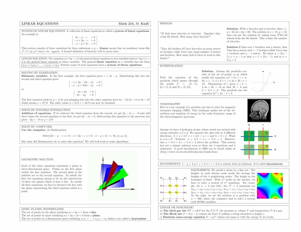
GEOMETRIC SOLUTION.

Each of the three equations represents a plane inthree-dimensional space. Points on the first planesatisfy the first equation. The second plane is thesolution set to the second equation. To satisfy thefirst two equations means to be on the intersectionof these two planes which is here a line. To satisfyall three equations, we have to intersect the line withthe plane representing the third equation which is apoint.

LINES, PLANES, HYPERPLANES.The set of points in the plane satisfying ax+ by = c form a line.The set of points in space satisfying ax+ by + cd = d form a plane.The set of points in n-dimensional space satisfying a1x1 + ...+ anxn = a0 define a set called a hyperplane.

RIDDLES:

”25 kids have bicycles or tricycles. Together theycount 60 wheels. How many have bicycles?”

Solution. With x bicycles and y tricycles, then x+y = 25, 2x+3y = 60. The solution is x = 15, y = 10.One can get the solution by taking away 2*25=50wheels from the 60 wheels. This counts the numberof tricycles.

”Tom, the brother of Carry has twice as many sistersas brothers while Carry has equal number of sistersand brothers. How many kids is there in total in thisfamily?”

Solution If there are x brothers and y sisters, thenTom has y sisters and x−1 brothers while Carry hasx brothers and y − 1 sisters. We know y = 2(x −1), x = y − 1 so that x + 1 = 2(x − 1) and so x =3, y = 4.

INTERPOLATION.

Find the equation of theparabola which passes throughthe points P = (0,−1),Q = (1, 4) and R = (2, 13).

Solution. Assume the parabola con-sists of the set of points (x, y) whichsatisfy the equation ax2 + bx + c = y.So, c = −1, a+ b+ c = 4, 4a+ 2b+ c =13. Elimination of c gives a + b =5, 4a + 2b = 14 so that 2b = 6 andb = 3, a = 2. The parabola has theequation 2x2 + 3x− 1 = 0

TOMOGRAPHYHere is a toy example of a problem one has to solve for magneticresonance imaging (MRI). This technique makes use of the ab-sorbtion and emission of energy in the radio frequency range ofthe electromagnetic spectrum.

Assume we have 4 hydrogen atoms, whose nuclei are excited withenergy intensity a, b, c, d. We measure the spin echo in 4 differentdirections. 3 = a + b,7 = c + d,5 = a + c and 5 = b + d. Whatis a, b, c, d? Solution: a = 2, b = 1, c = 3, d = 4. However,also a = 0, b = 3, c = 5, d = 2 solves the problem. This systemhas not a unique solution even so there are 4 equations and 4unknowns. A good introduction to MRI can be found online at(http://www.cis.rit.edu/htbooks/mri/inside.htm).

o

p

q r

a b

c d

INCONSISTENT. x− y = 4, y + z = 5, x+ z = 6 is a system with no solutions. It is called inconsistent.

x11 x12

x21 x22

a11 a12 a13 a14

a21 a24

a31 a34

a41 a42 a43 a44

EQUILIBRIUM. We model a drum by a fine net. Theheights at each interior node needs the average theheights of the 4 neighboring nodes. The height at theboundary is fixed. With n2 nodes in the interior, wehave to solve a system of n2 equations. For exam-ple, for n = 2 (see left), the n2 = 4 equations are4x11 = a21+a12+x21+x12, 4x12 = x11+x13+x22+x22,4x21 = x31+x11+x22+a43, 4x22 = x12+x21+a43+a34.To the right, we see the solution to a problem withn = 300, where the computer had to solve a systemwith 90′000 variables.

LINEAR OR NONLINEAR?a) The ideal gas law PV = nKT for the P, V, T , the pressure p, volume V and temperature T of a gas.b) The Hook law F = k(x− a) relates the force F pulling a string extended to length x.c) Einsteins mass-energy equation E = mc2 relates rest mass m with the energy E of a body.

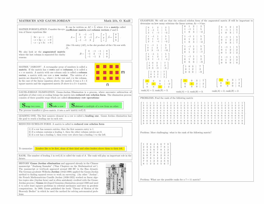
MATRICES AND GAUSS-JORDAN Math 21b, O. Knill

MATRIX FORMULATION. Consider the sys-tem of linear equations like

∣

∣

∣

∣

∣

∣

3x− y − z = 0−x+ 2y − z = 0−x− y + 3z = 9

∣

∣

∣

∣

∣

∣

It can be written as A~x = ~b, where A is a matrix calledcoefficient matrix and column vectors ~x and ~b.

A =

3 −1 −1−1 2 −1−1 −1 3

, ~x =

x

y

z

,~b =

009

.

(the i’th entry (A~x)i is the dot product of the i’th row with~x).

We also look at the augmented matrix

where the last column is separated for clarityreasons.

B =

3 −1 −1 | 0−1 2 −1 | 0−1 −1 3 | 9

.

MATRIX ”JARGON”. A rectangular array of numbers is called amatrix. If the matrix has n rows and m columns, it is called an×m matrix. A matrix with one column only is called a column

vector, a matrix with one row a row vector. The entries of amatrix are denoted by aij , where i is the row and j is the column.In the case of the linear equation above, the matrix A was a 3 × 3square matrix and the augmented matrix B above is a 3×4 matrix.

m

n

GAUSS-JORDAN ELIMINATION. Gauss-Jordan Elimination is a process, where successive subtraction ofmultiples of other rows or scaling brings the matrix into reduced row echelon form. The elimination processconsists of three possible steps which are called elementary row operations:

Swap two rows. Scale a row Subtract a multiple of a row from an other.

The process transfers a given matrix A into a new matrix rref(A)

LEADING ONE. The first nonzero element in a row is called a leading one. Gauss Jordan elimination hasthe goal to reach a leading one in each row.

REDUCED ECHELON FORM. A matrix is called in reduced row echelon form

1) if a row has nonzero entries, then the first nonzero entry is 1.2) if a column contains a leading 1, then the other column entries are 0.3) if a row has a leading 1, then every row above has a leading 1 to the left.

To memorize: Leaders like to be first, alone of their kind and other leaders above them to their left.

RANK. The number of leading 1 in rref(A) is called the rank of A. The rank will play an important role in thefuture.

HISTORY Gauss Jordan elimination and appeared already in the Chinesemanuscript ”Jiuzhang Suanshu” (’Nine Chapters on the Mathematical art’).The manuscript or textbook appeared around 200 BC in the Han dynasty.The German geodesist Wilhelm Jordan (1842-1899) applied the Gauss-Jordanmethod to finding squared errors to work on surveying. (An other ”Jordan”,the French Mathematician Camille Jordan (1838-1922) worked on linear alge-bra topics also (Jordan form) and is often mistakenly credited with the Gauss-Jordan process.) Gauss developed Gaussian elimination around 1800 and usedit to solve least squares problems in celestial mechanics and later in geodesiccomputations. In 1809, Gauss published the book ”Theory of Motion of theHeavenly Bodies” in which he used the method for solving astronomical prob-lems.

EXAMPLES. We will see that the reduced echelon form of the augmented matrix B will be important todetermine on how many solutions the linear system Ax = b has.

[

0 1 2 | 2

1 −1 1 | 5

2 1 −1 | −2

]

[

1 −1 1 | 5

0 1 2 | 2

2 1 −1 | −2

]

[

1 −1 1 | 5

0 1 2 | 2

0 3 −3 | −12

]

[

1 −1 1 | 5

0 1 2 | 2

0 1 −1 | −4

]

[

1 0 3 | 7

0 1 2 | 2

0 0 −3 | −6

]

[

1 0 3 | 7

0 1 2 | 2

0 0 1 | 2

]

1 0 0 | 1

0 1 0 | −2

0 0 1 | 2

rank(A) = 3, rank(B) = 3.

0 1 2 | 21 −1 1 | 51 0 3 | −2

1 −1 1 | 50 1 2 | 21 0 3 | −2

1 −1 1 | 50 1 2 | 20 1 2 | −7

1 −1 1 | 50 1 2 | 20 0 0 | −9

1 0 3 | 70 1 2 | 20 0 0 | −9

1 0 3 | 7

0 1 2 | 20 0 0 | 1

rank(A) = 2, rank(B) = 3.

0 1 2 | 21 −1 1 | 51 0 3 | 7

1 −1 1 | 50 1 2 | 21 0 3 | 7

1 −1 1 | 50 1 2 | 20 1 2 | 2

1 −1 1 | 50 1 2 | 20 0 0 | 0

1 0 3 | 7

0 1 2 | 20 0 0 | 0

rank(A) = 2, rank(B) = 2.

PROBLEMS. Find the rank of the following matrix

1 1 1 1 1 1 1 1 1 1 1 1 1 1 1 1 1 1 1 1 1 1 1 1 1 1 1 1 1 1

2 2 2 2 2 2 2 2 2 2 2 2 2 2 2 2 2 2 2 2 2 2 2 2 2 2 2 2 2 2

3 3 3 3 3 3 3 3 3 3 3 3 3 3 3 3 3 3 3 3 3 3 3 3 3 3 3 3 3 3

4 4 4 4 4 4 4 4 4 4 4 4 4 4 4 4 4 4 4 4 4 4 4 4 4 4 4 4 4 4

5 5 5 5 5 5 5 5 5 5 5 5 5 5 5 5 5 5 5 5 5 5 5 5 5 5 5 5 5 5

6 6 6 6 6 6 6 6 6 6 6 6 6 6 6 6 6 6 6 6 6 6 6 6 6 6 6 6 6 6

7 7 7 7 7 7 7 7 7 7 7 7 7 7 7 7 7 7 7 7 7 7 7 7 7 7 7 7 7 7

8 8 8 8 8 8 8 8 8 8 8 8 8 8 8 8 8 8 8 8 8 8 8 8 8 8 8 8 8 8

9 9 9 9 9 9 9 9 9 9 9 9 9 9 9 9 9 9 9 9 9 9 9 9 9 9 9 9 9 9

.

Problem: More challenging: what is the rank of the following matrix?

1 2 3 4 5 6 7 82 3 4 5 6 7 8 13 4 5 6 7 8 1 24 5 6 7 8 1 2 35 6 7 8 1 2 3 46 7 8 1 2 3 4 57 8 1 2 3 4 5 68 1 2 3 4 5 6 7

.

Problem: What are the possible ranks for a 7× 11 matrix?

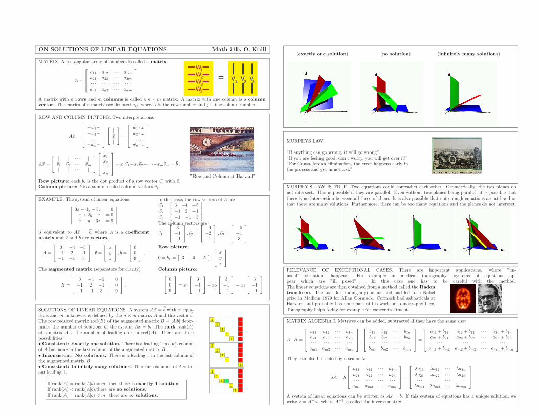
ON SOLUTIONS OF LINEAR EQUATIONS Math 21b, O. Knill

MATRIX. A rectangular array of numbers is called a matrix.

A =

a11 a12 · · · a1ma21 a22 · · · a2m· · · · · · · · · · · ·an1 an2 · · · anm

=wwww

v v v1

2

3

4

1 2 3

A matrix with n rows and m columns is called a n × m matrix. A matrix with one column is a column

vector. The entries of a matrix are denoted aij , where i is the row number and j is the column number.

ROW AND COLUMN PICTURE. Two interpretations

A~x =

−~w1−−~w2−. . .

−~wn−

|~x

|

=

~w1 · ~x~w2 · ~x. . .

~wn · ~x

A~x =

| | · · · |~v1 ~v2 · · · ~vm| | · · · |

x1

x2

· · ·xn

= x1~v1+x2~v2+· · ·+xm~vm = ~b .

Row picture: each bi is the dot product of a row vector ~wi with ~x.Column picture: ~b is a sum of scaled column vectors ~vj .

”Row and Column at Harvard”

EXAMPLE. The system of linear equations

∣

∣

∣

∣

∣

∣

3x− 4y − 5z = 0−x+ 2y − z = 0−x− y + 3z = 9

∣

∣

∣

∣

∣

∣

is equivalent to A~x = ~b, where A is a coefficient

matrix and ~x and ~b are vectors.

A =

3 −4 −5−1 2 −1−1 −1 3

, ~x =

x

y

z

,~b =

009

.

The augmented matrix (separators for clarity)

B =

3 −4 −5 | 0−1 2 −1 | 0−1 −1 3 | 9

.

In this case, the row vectors of A are~w1 =

[

3 −4 −5]

~w2 =[

−1 2 −1]

~w3 =[

−1 −1 3]

The column vectors are

~v1 =

3−1−1

, ~v2 =

−4−2−1

, ~v3 =

−5−13

Row picture:

0 = b1 =[

3 −4 −5]

·

x

y

z

Column picture:

009

= x1

3−1−1

+ x2

3−1−1

+ x3

3−1−1

SOLUTIONS OF LINEAR EQUATIONS. A system A~x = ~b with n equa-tions and m unknowns is defined by the n×m matrix A and the vector ~b.The row reduced matrix rref(B) of the augmented matrix B = [A|b] deter-mines the number of solutions of the system Ax = b. The rank rank(A)of a matrix A is the number of leading ones in rref(A). There are threepossibilities:• Consistent: Exactly one solution. There is a leading 1 in each columnof A but none in the last column of the augmented matrix B.• Inconsistent: No solutions. There is a leading 1 in the last column ofthe augmented matrix B.• Consistent: Infinitely many solutions. There are columns of A with-out leading 1.

If rank(A) = rank(A|b) = m, then there is exactly 1 solution.If rank(A) < rank(A|b),there are no solutions.If rank(A) = rank(A|b) < m: there are ∞ solutions.

1

11

1

1

1

11

1

1

1

11

11

(exactly one solution) (no solution) (infinitely many solutions)

MURPHYS LAW.

”If anything can go wrong, it will go wrong”.”If you are feeling good, don’t worry, you will get over it!””For Gauss-Jordan elimination, the error happens early inthe process and get unnoticed.”

MURPHY’S LAW IS TRUE. Two equations could contradict each other. Geometrically, the two planes donot intersect. This is possible if they are parallel. Even without two planes being parallel, it is possible thatthere is no intersection between all three of them. It is also possible that not enough equations are at hand orthat there are many solutions. Furthermore, there can be too many equations and the planes do not intersect.

RELEVANCE OF EXCEPTIONAL CASES. There are important applications, where ”un-usual” situations happen: For example in medical tomography, systems of equations ap-pear which are ”ill posed”. In this case one has to be careful with the method.The linear equations are then obtained from a method called the Radon

transform. The task for finding a good method had led to a Nobelprize in Medicin 1979 for Allan Cormack. Cormack had sabbaticals atHarvard and probably has done part of his work on tomography here.Tomography helps today for example for cancer treatment.

MATRIX ALGEBRA I. Matrices can be added, subtracted if they have the same size:

A+B =

a11 a12 · · · a1na21 a22 · · · a2n· · · · · · · · · · · ·am1 am2 · · · amn

+

b11 b12 · · · b1nb21 b22 · · · b2n· · · · · · · · · · · ·bm1 bm2 · · · bmn

=

a11 + b11 a12 + b12 · · · a1n + b1na21 + b21 a22 + b22 · · · a2n + b2n

· · · · · · · · · · · ·am1 + bm2 am2 + bm2 · · · amn + bmn

They can also be scaled by a scalar λ:

λA = λ

a11 a12 · · · a1na21 a22 · · · a2n· · · · · · · · · · · ·am1 am2 · · · amn

=

λa11 λa12 · · · λa1nλa21 λa22 · · · λa2n· · · · · · · · · · · ·

λam1 λam2 · · · λamn

A system of linear equations can be written as Ax = b. If this system of equations has a unique solution, wewrite x = A−1b, where A−1 is called the inverse matrix.

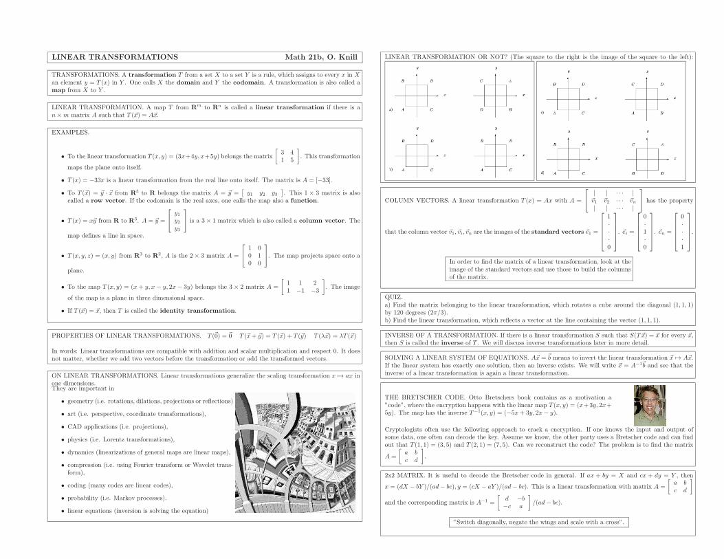
LINEAR TRANSFORMATIONS Math 21b, O. Knill

TRANSFORMATIONS. A transformation T from a set X to a set Y is a rule, which assigns to every x in Xan element y = T (x) in Y . One calls X the domain and Y the codomain. A transformation is also called amap from X to Y .

LINEAR TRANSFORMATION. A map T from Rm to Rn is called a linear transformation if there is an×m matrix A such that T (~x) = A~x.

EXAMPLES.

• To the linear transformation T (x, y) = (3x+4y, x+5y) belongs the matrix

[

3 41 5

]

. This transformation

maps the plane onto itself.

• T (x) = −33x is a linear transformation from the real line onto itself. The matrix is A = [−33].

• To T (~x) = ~y · ~x from R3 to R belongs the matrix A = ~y =[

y1 y2 y3]

. This 1 × 3 matrix is alsocalled a row vector. If the codomain is the real axes, one calls the map also a function.

• T (x) = x~y from R to R3. A = ~y =

y1y2y3

is a 3× 1 matrix which is also called a column vector. The

map defines a line in space.

• T (x, y, z) = (x, y) from R3 to R2, A is the 2 × 3 matrix A =

1 00 10 0

. The map projects space onto a

plane.

• To the map T (x, y) = (x + y, x − y, 2x− 3y) belongs the 3 × 2 matrix A =

[

1 1 21 −1 −3

]

. The image

of the map is a plane in three dimensional space.

• If T (~x) = ~x, then T is called the identity transformation.

PROPERTIES OF LINEAR TRANSFORMATIONS. T (~0) = ~0 T (~x+ ~y) = T (~x) + T (~y) T (λ~x) = λT (~x)

In words: Linear transformations are compatible with addition and scalar multiplication and respect 0. It doesnot matter, whether we add two vectors before the transformation or add the transformed vectors.

ON LINEAR TRANSFORMATIONS. Linear transformations generalize the scaling transformation x 7→ ax inone dimensions.They are important in

• geometry (i.e. rotations, dilations, projections or reflections)

• art (i.e. perspective, coordinate transformations),

• CAD applications (i.e. projections),

• physics (i.e. Lorentz transformations),

• dynamics (linearizations of general maps are linear maps),

• compression (i.e. using Fourier transform or Wavelet trans-form),

• coding (many codes are linear codes),

• probability (i.e. Markov processes).

• linear equations (inversion is solving the equation)

LINEAR TRANSFORMATION OR NOT? (The square to the right is the image of the square to the left):

COLUMN VECTORS. A linear transformation T (x) = Ax with A =

| | · · · |~v1 ~v2 · · · ~vn| | · · · |

has the property

that the column vector ~v1, ~vi, ~vn are the images of the standard vectors ~e1 =

1···0

. ~ei =

0·1·0

. ~en =

0···1

.

In order to find the matrix of a linear transformation, look at theimage of the standard vectors and use those to build the columnsof the matrix.

QUIZ.a) Find the matrix belonging to the linear transformation, which rotates a cube around the diagonal (1, 1, 1)by 120 degrees (2π/3).b) Find the linear transformation, which reflects a vector at the line containing the vector (1, 1, 1).

INVERSE OF A TRANSFORMATION. If there is a linear transformation S such that S(T~x) = ~x for every ~x,then S is called the inverse of T . We will discuss inverse transformations later in more detail.

SOLVING A LINEAR SYSTEM OF EQUATIONS. A~x = ~b means to invert the linear transformation ~x 7→ A~x.If the linear system has exactly one solution, then an inverse exists. We will write ~x = A−1~b and see that theinverse of a linear transformation is again a linear transformation.

THE BRETSCHER CODE. Otto Bretschers book contains as a motivation a”code”, where the encryption happens with the linear map T (x, y) = (x+3y, 2x+5y). The map has the inverse T−1(x, y) = (−5x+ 3y, 2x− y).

Cryptologists often use the following approach to crack a encryption. If one knows the input and output ofsome data, one often can decode the key. Assume we know, the other party uses a Bretscher code and can findout that T (1, 1) = (3, 5) and T (2, 1) = (7, 5). Can we reconstruct the code? The problem is to find the matrix

A =

[

a bc d

]

.

2x2 MATRIX. It is useful to decode the Bretscher code in general. If ax + by = X and cx + dy = Y , then

x = (dX − bY )/(ad− bc), y = (cX − aY )/(ad− bc). This is a linear transformation with matrix A =

[

a bc d

]

and the corresponding matrix is A−1 =

[

d −b−c a

]

/(ad− bc).

”Switch diagonally, negate the wings and scale with a cross”.

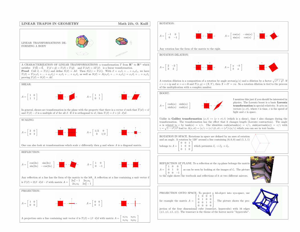
LINEAR TRAFOS IN GEOMETRY Math 21b, O. Knill

LINEAR TRANSFORMATIONS DE-FORMING A BODY

A CHARACTERIZATION OF LINEAR TRANSFORMATIONS: a transformation T from Rn to R

m whichsatisfies T (~0) = ~0, T (~x+ ~y) = T (~x) + T (~y) and T (λ~x) = λT (~x) is a linear transformation.Proof. Call ~vi = T (~ei) and define S(~x) = A~x. Then S(~ei) = T (~ei). With ~x = x1~e1 + ... + xn~en, we haveT (~x) = T (x1~e1 + ... + xn~en) = x1~v1 + ... + xn~vn as well as S(~x) = A(x1~e1 + ... + xn~en) = x1~v1 + ... + xn~vnproving T (~x) = S(~x) = A~x.

SHEAR:

A =

[

1 01 1

]

A =

[

1 10 1

]

In general, shears are transformation in the plane with the property that there is a vector ~w such that T (~w) = ~wand T (~x)− ~x is a multiple of ~w for all ~x. If ~u is orthogonal to ~w, then T (~x) = ~x+ (~u · ~x)~w.

SCALING:

A =

[

2 00 2

]

A =

[

1/2 00 1/2

]

One can also look at transformations which scale x differently then y and where A is a diagonal matrix.

REFLECTION:

A =

[

cos(2α) sin(2α)sin(2α) − cos(2α)

]

A =

[

1 00 −1

]

Any reflection at a line has the form of the matrix to the left. A reflection at a line containing a unit vector ~u

is T (~x) = 2(~x · ~u)~u− ~x with matrix A =

[

2u2

1− 1 2u1u2

2u1u2 2u2

2− 1

]

PROJECTION:

A =

[

1 00 0

]

A =

[

0 00 1

]

A projection onto a line containing unit vector ~u is T (~x) = (~x · ~u)~u with matrix A =

[

u1u1 u2u1

u1u2 u2u2

]

ROTATION:

A =

[

−1 00 −1

]

A =

[

cos(α) − sin(α)sin(α) cos(α)

]

Any rotation has the form of the matrix to the right.

ROTATION-DILATION:

A =

[

2 −33 2

]

A =

[

a −bb a

]

A rotation dilation is a composition of a rotation by angle arctan(y/x) and a dilation by a factor√

x2 + y2. Ifz = x+ iy and w = a+ ib and T (x, y) = (X,Y ), then X+ iY = zw. So a rotation dilation is tied to the processof the multiplication with a complex number.

BOOST:

A =

[

cosh(α) sinh(α)sinh(α) cosh(α)

]

I mention this just if you should be interested inphysics. The Lorentz boost is a basic Lorentz

transformation in special relativity. It acts onvectors (x, ct), where t is time, c is the speed oflight and x is space.

Unlike in Galileo transformation (x, t) 7→ (x + vt, t) (which is a shear), time t also changes during thetransformation. The transformation has the effect that it changes length (Lorentz contraction). The angleα is related to v by tanh(α) = v/c. The identities cosh(artanh(α) = v/γ, sinh(arctanh(α)) = v/γ withγ =

√

1− v2/c2 lead to A(x, ct) = (x/γ + (v/γ)t, ctγ + (v2/c)x/γ) which you can see in text books.

ROTATION IN SPACE. Rotations in space are defined by an axes of rotationand an angle. A rotation by 120◦ around a line containing (0, 0, 0) and (1, 1, 1)

belongs to A =

0 0 11 0 00 1 0

which permutes ~e1 → ~e2 → ~e3.

REFLECTION AT PLANE. To a reflection at the xy-plane belongs the matrix

A =

1 0 00 1 00 0 −1

as can be seen by looking at the images of ~ei. The picture

to the right shows the textbook and reflections of it at two different mirrors.

PROJECTION ONTO SPACE. To project a 4d-object into xyz-space, use

for example the matrix A =

1 0 0 00 1 0 00 0 1 00 0 0 0

. The picture shows the pro-

jection of the four dimensional cube (tesseract, hypercube) with 16 edges(±1,±1,±1,±1). The tesseract is the theme of the horror movie ”hypercube”.

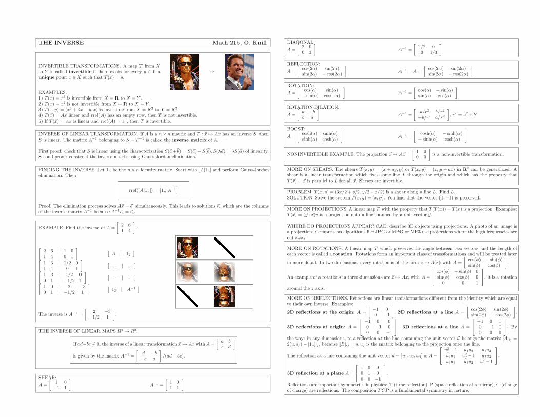
THE INVERSE Math 21b, O. Knill

INVERTIBLE TRANSFORMATIONS. A map T from Xto Y is called invertible if there exists for every y ∈ Y aunique point x ∈ X such that T (x) = y.

⇒

EXAMPLES.1) T (x) = x3 is invertible from X = R to X = Y .2) T (x) = x2 is not invertible from X = R to X = Y .3) T (x, y) = (x2 + 3x− y, x) is invertible from X = R2 to Y = R2.4) T (~x) = Ax linear and rref(A) has an empty row, then T is not invertible.5) If T (~x) = Ax is linear and rref(A) = 1n, then T is invertible.

INVERSE OF LINEAR TRANSFORMATION. If A is a n× n matrix and T : ~x 7→ Ax has an inverse S, thenS is linear. The matrix A−1 belonging to S = T−1 is called the inverse matrix of A.

First proof: check that S is linear using the characterization S(~a+~b) = S(~a)+S(~b), S(λ~a) = λS(~a) of linearity.Second proof: construct the inverse matrix using Gauss-Jordan elimination.

FINDING THE INVERSE. Let 1n be the n× n identity matrix. Start with [A|1n] and perform Gauss-Jordanelimination. Then

rref([A|1n]) =[

1n|A−1

]

Proof. The elimination process solves A~x = ~ei simultaneously. This leads to solutions ~vi which are the columnsof the inverse matrix A−1 because A−1~ei = ~vi.

EXAMPLE. Find the inverse of A =

[

2 61 4

]

.

[

2 6 | 1 01 4 | 0 1

]

[

A | 12]

[

1 3 | 1/2 01 4 | 0 1

]

[

.... | ...]

[

1 3 | 1/2 00 1 | −1/2 1

]

[

.... | ...]

[

1 0 | 2 −30 1 | −1/2 1

]

[

12 | A−1]

The inverse is A−1 =

[

2 −3−1/2 1

]

.

THE INVERSE OF LINEAR MAPS R2 7→ R2:

If ad−bc 6= 0, the inverse of a linear transformation ~x 7→ Ax with A =

[

a bc d

]

is given by the matrix A−1 =

[

d −b−c a

]

/(ad− bc).

SHEAR:

A =

[

1 0−1 1

]

A−1 =

[

1 01 1

]

DIAGONAL:

A =

[

2 00 3

]

A−1 =

[

1/2 00 1/3

]

REFLECTION:

A =

[

cos(2α) sin(2α)sin(2α) − cos(2α)

]

A−1 = A =

[

cos(2α) sin(2α)sin(2α) − cos(2α)

]

ROTATION:

A =

[

cos(α) sin(α)− sin(α) cos(−α)

]

A−1 =

[

cos(α) − sin(α)sin(α) cos(α)

]

ROTATION-DILATION:

A =

[

a −bb a

]

A−1 =

[

a/r2 b/r2

−b/r2 a/r2

]

, r2 = a2 + b2

BOOST:

A =

[

cosh(α) sinh(α)sinh(α) cosh(α)

]

A−1 =

[

cosh(α) − sinh(α)− sinh(α) cosh(α)

]

NONINVERTIBLE EXAMPLE. The projection ~x 7→ A~x =

[

1 00 0

]

is a non-invertible transformation.

MORE ON SHEARS. The shears T (x, y) = (x + ay, y) or T (x, y) = (x, y + ax) in R2 can be generalized. Ashear is a linear transformation which fixes some line L through the origin and which has the property thatT (~x)− ~x is parallel to L for all ~x. Shears are invertible.

PROBLEM. T (x, y) = (3x/2 + y/2, y/2− x/2) is a shear along a line L. Find L.SOLUTION. Solve the system T (x, y) = (x, y). You find that the vector (1,−1) is preserved.

MORE ON PROJECTIONS. A linear map T with the property that T (T (x)) = T (x) is a projection. Examples:T (~x) = (~y · ~x)~y is a projection onto a line spanned by a unit vector ~y.

WHERE DO PROJECTIONS APPEAR? CAD: describe 3D objects using projections. A photo of an image isa projection. Compression algorithms like JPG or MPG or MP3 use projections where the high frequencies arecut away.

MORE ON ROTATIONS. A linear map T which preserves the angle between two vectors and the length ofeach vector is called a rotation. Rotations form an important class of transformations and will be treated later

in more detail. In two dimensions, every rotation is of the form x 7→ A(x) with A =

[

cos(φ) − sin(φ)sin(φ) cos(φ)

]

.

An example of a rotations in three dimensions are ~x 7→ Ax, with A =

cos(φ) − sin(φ) 0sin(φ) cos(φ) 0

0 0 1

. it is a rotation

around the z axis.

MORE ON REFLECTIONS. Reflections are linear transformations different from the identity which are equalto their own inverse. Examples:

2D reflections at the origin: A =

[

−1 00 −1

]

, 2D reflections at a line A =

[

cos(2φ) sin(2φ)sin(2φ) − cos(2φ)

]

.

3D reflections at origin: A =

−1 0 00 −1 00 0 −1

. 3D reflections at a line A =

−1 0 00 −1 00 0 1

. By

the way: in any dimensions, to a reflection at the line containing the unit vector ~u belongs the matrix [A]ij =2(uiuj)− [1n]ij , because [B]ij = uiuj is the matrix belonging to the projection onto the line.

The reflection at a line containing the unit vector ~u = [u1, u2, u3] is A =

u2

1− 1 u1u2 u1u3

u2u1 u2

2− 1 u2u3

u3u1 u3u2 u2

3− 1

.

3D reflection at a plane A =

1 0 00 1 00 0 −1

.

Reflections are important symmetries in physics: T (time reflection), P (space reflection at a mirror), C (changeof charge) are reflections. The composition TCP is a fundamental symmetry in nature.

MATRIX PRODUCT Math 21b, O. Knill

MATRIX PRODUCT. If A is a n × m matrix and A is a m ×p matrix, then AB is defined as the n × p matrix with entries(BA)ij =

∑m

k=1BikAkj . It represents a linear transformation

from Rp → Rn where first B is applied as a map from Rp → Rm

and then the transformation A from Rm → Rn.

EXAMPLE. If B is a 3× 4 matrix, and A is a 4× 2 matrix then BA is a 3× 2 matrix.

B =

1 3 5 73 1 8 11 0 9 2

, A =

1 33 11 00 1

, BA =

1 3 5 73 1 8 11 0 9 2

1 33 11 00 1

=

15 1314 1110 5

.

COMPOSING LINEAR TRANSFORMATIONS. If T : Rp → Rm, x 7→ Bx and S : Rm → Rn, y 7→ Ay arelinear transformations, then their composition S ◦ T : x 7→ A(B(x)) = ABx is a linear transformation from Rp

to Rn. The corresponding n× p matrix is the matrix product AB.

EXAMPLE. Find the matrix which is a composition of a rotation around the x-axes by an angle π/2 followedby a rotation around the z-axes by an angle π/2.SOLUTION. The first transformation has the property that e1 → e1, e2 → e3, e3 → −e2, the second e1 →e2, e2 → −e1, e3 → e3. If A is the matrix belonging to the first transformation and B the second, then BAis the matrix to the composition. The composition maps e1 → −e2 → e3 → e1 is a rotation around a long

diagonal. B =

0 −1 01 0 00 0 1

A =

1 0 00 0 −10 1 0

, BA =

0 0 11 0 00 1 0

.

EXAMPLE. A rotation dilation is the composition of a rotation by α = arctan(b/a) and a dilation (=scale) byr =

√a2 + b2.

REMARK. Matrix multiplication can be seen a generalization of usual multiplication of numbers and alsogeneralizes the dot product.

MATRIX ALGEBRA. Note that AB 6= BA in general and A−1 does not always exist, otherwise, the same rulesapply as for numbers:A(BC) = (AB)C, AA−1 = A−1A = 1n, (AB)−1 = B−1A−1, A(B + C) = AB + AC, (B + C)A = BA + CAetc.

PARTITIONED MATRICES. The entries of matrices can themselves be matrices. If B is a n × p matrix andA is a p×m matrix, and assume the entries are k × k matrices, then BA is a n×m matrix, where each entry(BA)ij =

∑p

l=1BilAlj is a k × k matrix. Partitioning matrices can be useful to improve the speed of matrix

multiplication

EXAMPLE. If A =

[

A11 A12

0 A22

]

, where Aij are k × k matrices with the property that A11 and A22 are

invertible, then B =

[

A−1

11−A−1

11A12A

−1

22

0 A−1

22

]

is the inverse of A.

The material which follows is for motivation purposes only:

1

4

2

3

NETWORKS. Let us associate to the computer network a matrix

0 1 1 11 0 1 01 1 0 11 0 1 0

A worm in the first computer is associated to

1000

. The

vector Ax has a 1 at the places, where the worm could be in the next step. Thevector (AA)(x) tells, in how many ways the worm can go from the first computerto other hosts in 2 steps. In our case, it can go in three different ways back to thecomputer itself.Matrices help to solve combinatorial problems (see movie ”Good will hunting”).For example, what does [A1000]22 tell about the worm infection of the network?What does it mean if A100 has no zero entries?

FRACTALS. Closely related to linear maps are affine maps x 7→ Ax + b. They are compositions of a linearmap with a translation. It is not a linear map if B(0) 6= 0. Affine maps can be disguised as linear maps

in the following way: let y =

[

x1

]

and defne the (n+1)∗(n+1) matrix B =

[

A b0 1

]

. Then By =

[

Ax + b1

]

.

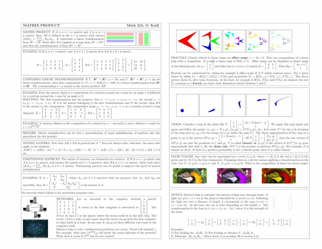
Fractals can be constructed by taking for example 3 affine maps R,S, T which contract space. For a givenobject Y0 define Y1 = R(Y0) ∪ S(Y0) ∪ T (Y0) and recursively Yk = R(Yk−1) ∪ S(Yk−1) ∪ T (Yk−1). The abovepicture shows Yk after some iterations. In the limit, for example if R(Y0), S(Y0) and T (Y0) are disjoint, the setsYk converge to a fractal, an object with dimension strictly between 1 and 2.

CHAOS. Consider a map in the plane like T :

[

xy

]

7→[

2x+ 2 sin(x) − yx

]

. We apply this map again and

again and follow the points (x1, y1) = T (x, y), (x2, y2) = T (T (x, y)), etc. Lets write T n for the n-th iterationof the map and (xn, yn) for the image of (x, y) under the map T n. The linear approximation of the map at a

point (x, y) is the matrix DT (x, y) =

[

2 + 2 cos(x)− 11

]

. (If T

[

xy

]

=

[

f(x, y)g(x, y)

]

, then the row vectors of

DT (x, y) are just the gradients of f and g). T is called chaotic at (x, y), if the entries of D(T n)(x, y) growexponentially fast with n. By the chain rule, D(T n) is the product of matrices DT (xi, yi). For example, T ischaotic at (0, 0). If there is a positive probability to hit a chaotic point, then T is called chaotic.

FALSE COLORS. Any color can be represented as a vector (r, g, b), where r ∈ [0, 1] is the red g ∈ [0, 1] is thegreen and b ∈ [0, 1] is the blue component. Changing colors in a picture means applying a transformation on thecube. Let T : (r, g, b) 7→ (g, b, r) and S : (r, g, b) 7→ (r, g, 0). What is the composition of these two linear maps?

OPTICS. Matrices help to calculate the motion of light rays through lenses. Alight ray y(s) = x+ms in the plane is described by a vector (x,m). Followingthe light ray over a distance of length L corresponds to the map (x,m) 7→(x + mL,m). In the lens, the ray is bent depending on the height x. Thetransformation in the lens is (x,m) 7→ (x,m − kx), where k is the strength ofthe lense.

[

xm

]

7→ AL

[

xm

]

=

[

1 L0 1

] [

xm

]

,

[

xm

]

7→ Bk

[

xm

]

=

[

1 0−k 1

] [

xm

]

.

Examples:1) Eye looking far: ARBk. 2) Eye looking at distance L: ARBkAL.3) Telescope: Bk2

ALBk1. (More about it in problem 80 in section 2.4).

IMAGE AND KERNEL Math 21b, O. Knill

IMAGE. If T : Rm → Rn is a linear transformation, then {T (~x) | ~x ∈ Rm } is called the image of T . IfT (~x) = A~x, then the image of T is also called the image of A. We write im(A) or im(T ).

EXAMPLES.1) The map T (x, y, z) = (x, y, 0) maps space into itself. It is linear because we can find a matrix A for which

T (~x) = A

x

y

z

=

1 0 00 1 00 0 0

x

y

z

. The image of T is the x− y plane.

2) If T (x, y) = (cos(φ)x− sin(φ)y, sin(φ)x+cos(φ)y) is a rotation in the plane, then the image of T is the wholeplane.3) If T (x, y, z) = x+ y + z, then the image of T is R.

SPAN. The span of vectors ~v1, . . . , ~vk in Rn is the set of all combinations c1~v1 + . . . ck~vk, where ci are realnumbers.

PROPERTIES.The image of a linear transformation ~x 7→ A~x is the span of the column vectors of A.The image of a linear transformation contains 0 and is closed under addition and scalar multiplication.

KERNEL. If T : Rm → Rn is a linear transformation, then the set {x | T (x) = 0 } is called the kernel of T .If T (~x) = A~x, then the kernel of T is also called the kernel of A. We write ker(A) or ker(T ).

EXAMPLES. (The same examples as above)1) The kernel is the z-axes. Every vector (0, 0, z) is mapped to 0.2) The kernel consists only of the point (0, 0, 0).3) The kernel consists of all vector (x, y, z) for which x+ y + z = 0. The kernel is a plane.

PROPERTIES.The kernel of a linear transformation contains 0 and is closed under addition and scalar multiplication.

IMAGE AND KERNEL OF INVERTIBLE MAPS. A linear map ~x 7→ A~x, Rn 7→ Rn is invertible if and onlyif ker(A) = {~0} if and only if im(A) = Rn.

HOW DO WE COMPUTE THE IMAGE? The column vectors of A span the image. We will see later that thecolumns with leading ones alone span already the image.

EXAMPLES. (The same examples as above)

1)

100

and

010

span the image.

2)

[

cos(φ)− sin(φ)

]

and

[

sin(φ)cos(φ)

]

span the image.

3) The 1D vector[

1]

spans theimage.

HOW DO WE COMPUTE THE KERNEL? Just solve the linear system of equations A~x = ~0. Form rref(A).For every column without leading 1 we can introduce a free variable si. If ~x is the solution to A~xi = 0, whereall sj are zero except si = 1, then ~x =

∑

j sj~xj is a general vector in the kernel.

EXAMPLE. Find the kernel of the linear map R3 → R4, ~x 7→ A~x with A =

1 3 02 6 53 9 1−2 −6 0

. Gauss-Jordan

elimination gives: B = rref(A) =

1 3 00 0 10 0 00 0 0

. We see one column without leading 1 (the second one). The

equation B~x = 0 is equivalent to the system x + 3y = 0, z = 0. After fixing z = 0, can chose y = t freely and

obtain from the first equation x = −3t. Therefore, the kernel consists of vectors t

−310

. In the book, you

have a detailed calculation, in a case, where the kernel is 2 dimensional.

domain

codomain

kernel

image

WHY DO WE LOOK AT THE KERNEL?

• It is useful to understand linear maps. To whichdegree are they non-invertible?

• Helpful to understand quantitatively how manysolutions a linear equation Ax = b has. If x isa solution and y is in the kernel of A, then alsoA(x + y) = b, so that x + y solves the systemalso.

WHY DO WE LOOK AT THE IMAGE?

• A solution Ax = b can be solved if and only if bis in the image of A.

• Knowing about the kernel and the image is use-ful in the similar way that it is useful to knowabout the domain and range of a general mapand to understand the graph of the map.

In general, the abstraction helps to understand topics like error correcting codes (Problem 53/54 in Bretscher’sbook), where two matrices H,M with the property that ker(H) = im(M) appear. The encoding x 7→ Mx isrobust in the sense that adding an error e to the result Mx 7→ Mx + e can be corrected: H(Mx + e) = He

allows to find e and so Mx. This allows to recover x = PMx with a projection P .

PROBLEM. Find ker(A) and im(A) for the 1× 3 matrix A = [5, 1, 4], a row vector.ANSWER. A · ~x = A~x = 5x+ y + 4z = 0 shows that the kernel is a plane with normal vector [5, 1, 4] throughthe origin. The image is the codomain, which is R.

PROBLEM. Find ker(A) and im(A) of the linear map x 7→ v × x, (the cross product with v.ANSWER. The kernel consists of the line spanned by v, the image is the plane orthogonal to v.

PROBLEM. Fix a vector w in space. Find ker(A) and image im(A) of the linear map from R6 to R3 given byx, y 7→ [x, v, y] = (x× y) · w.ANSWER. The kernel consist of all (x, y) such that their cross product orthogonal to w. This means that theplane spanned by x, y contains w.

PROBLEM Find ker(T ) and im(T ) if T is a composition of a rotation R by 90 degrees around the z-axes withwith a projection onto the x-z plane.ANSWER. The kernel of the projection is the y axes. The x axes is rotated into the y axes and therefore thekernel of T . The image is the x-z plane.

PROBLEM. Can the kernel of a square matrix A be trivial if A2 = 0, where 0 is the matrix containing only 0?ANSWER. No: if the kernel were trivial, then A were invertible and A2 were invertible and be different from 0.

PROBLEM. Is it possible that a 3× 3 matrix A satisfies ker(A) = R3 without A = 0?ANSWER. No, if A 6= 0, then A contains a nonzero entry and therefore, a column vector which is nonzero.

PROBLEM. What is the kernel and image of a projection onto the plane Σ : x− y + 2z = 0?ANSWER. The kernel consists of all vectors orthogonal to Σ, the image is the plane Σ.

PROBLEM. Given two square matrices A,B and assume AB = BA. You know ker(A) and ker(B). What canyou say about ker(AB)?ANSWER. ker(A) is contained in ker(BA). Similarly ker(B) is contained in ker(AB). Because AB = BA, the

kernel of AB contains both ker(A) and ker(B). (It can be bigger as the example A = B =

[

0 10 0

]

shows.)

PROBLEM. What is the kernel of the partitioned matrix

[

A 00 B

]

if ker(A) and ker(B) are known?

ANSWER. The kernel consists of all vectors (~x, ~y), where ~x in ker(A) and ~y ∈ ker(B).

BASIS Math 21b, O. Knill

LINEAR SUBSPACE: A subset X of Rn which is closed under addition and scalar multiplication is called alinear subspace of Rn. We have to check three conditions: (a) 0 ∈ V , (b) ~v + ~w ∈ V if ~v, ~w ∈ V . (b) λ~v ∈ V

if ~v and λ is a real number.

WHICH OF THE FOLLOWING SETS ARE LINEAR SPACES?

a) The kernel of a linear map.b) The image of a linear map.c) The upper half plane.d) The set x2 = y2.

e) the line x+ y = 0.f) The plane x+ y + z = 1.g) The unit circle.h) The x axes.

BASIS. A set of vectors ~v1, . . . , ~vm is a basis of a linear subspace X of Rn if they arelinear independent and if they span the space X . Linear independent means thatthere are no nontrivial linear relations ai~v1 + . . .+ am~vm = 0. Spanning the spacemeans that very vector ~v can be written as a linear combination ~v = a1~v1+ . . .+am~vmof basis vectors.

EXAMPLE 1) The vectors ~v1 =

110

, ~v2 =

011

, ~v3 =

101

form a basis in the three dimensional space.

If ~v =

435

, then ~v = ~v1 +2~v2 +3~v3 and this representation is unique. We can find the coefficients by solving

A~x = ~v, where A has the vi as column vectors. In our case, A =

1 0 11 1 00 1 1

x

y

z

=

435

had the unique

solution x = 1, y = 2, z = 3 leading to ~v = ~v1 + 2~v2 + 3~v3.

EXAMPLE 2) Two nonzero vectors in the plane which are not parallel form a basis.EXAMPLE 3) Four vectors in R3 are not a basis.EXAMPLE 4) Two vectors in R3 never form a basis.EXAMPLE 5) Three nonzero vectors in R3 which are not contained in a single plane form a basis in R3.EXAMPLE 6) The columns of an invertible n× n matrix form a basis in Rn.

FACT. If ~v1, . . . , ~vn is a basis, thenevery vector ~v can be representeduniquely as a linear combination of thebasis vectors: ~v = a1~v1 + · · ·+ an~vn.

REASON. There is at least one representation because the vectors~vi span the space. If there were two different representations ~v =a1~v1+ . . .+an~vn and ~v = b1~v1+ . . .+bn~vn, then subtraction wouldlead to 0 = (a1 − b1)~v1 + . . .+ (an − bn)~vn. Linear independenceshows a1 − b1 = a2 − b2 = ... = an − bn = 0.

FACT. If n vectors ~v1, ..., ~vn span a space and ~w1, ..., ~wm are linear independent, then m ≤ n.

REASON. This is intuitively clear in dimensions up to 3. You can not have 4 vectors in three dimensional spacewhich are linearly independent. We will give a precise reason later.

A BASIS DEFINES AN INVERTIBLE MATRIX. The n× n matrix A =

| | |~v1 ~v2 . . . ~vn| | |

is invertible if

and only if ~v1, . . . , ~vn define a basis in Rn.

EXAMPLE. In example 1), the 3× 3 matrix A is invertible.

FINDING A BASIS FOR THE KERNEL. To solve Ax = 0, we bring the matrix A into the reduced row echelonform rref(A). For every non-leading entry in rref(A), we will get a free variable ti. Writing the system Ax = 0with these free variables gives us an equation ~x =

∑

iti~vi. The vectors ~vi form a basis of the kernel of A.

REMARK. The problem to find a basis for all vectors ~wi which are orthogonal to a given set of vectors, isequivalent to the problem to find a basis for the kernel of the matrix which has the vectors ~wi in its rows.

FINDING A BASIS FOR THE IMAGE. Bring the m × n matrix A into the form rref(A). Call a column apivot column, if it contains a leading 1. The corresponding set of column vectors of the original matrix A

form a basis for the image because they are linearly independent and they all are in the image.The pivot columns also span the image because if we remove the nonpivot columns, and ~b is in the image, wecan solve A~x = b.

EXAMPLE. A =

[

1 2 3 4 51 3 3 4 5

]

. has two pivot columns, the first and second one. For ~b =

[

34

]

, we can

solve A~x = ~b. We can also solve B~x = ~b with B =

[

1 21 3

]

.

REMARK. The problem to find a basis of the subspace generated by ~v1, . . . , ~vn, is the problem to find a basisfor the image of the matrix A with column vectors ~v1, . . . , ~vn.

EXAMPLE. Let A be the matrix A =

∣

∣

∣

∣

∣

∣

0 0 11 1 01 1 1

∣

∣

∣

∣

∣

∣

. In reduced row echelon form is B = rref(A) =

∣

∣

∣

∣

∣

∣

1 1 00 0 10 0 0

∣

∣

∣

∣

∣

∣

.

To determine a basis of the kernel we write Bx = 0 as a system of linear equations: x + y = 0, z = 0. Thevariable y is the free variable. With y = t, x = −t is fixed. The linear system rref(A)x = 0 is solved by

~x =

x

y

z

= t

−110

. So, ~v =

−110

is a basis of the kernel.

EXAMPLE. Because the first and third vectors in rref(A) are columns with leading 1’s, the first and third

columns ~v1 =

011

, ~v2 =

101

of A form a basis of the image of A.

WHY DO WE INTRODUCE BASIS VECTORS? Wouldn’t it be justeasier to always look at the standard basis vectors ~e1, . . . , ~en only? Thereason for the need of more general basis vectors is that they allow a

more flexible adaptation to the situation. A person in Paris prefersa different set of basis vectors than a person in Boston. We will also seethat in many applications, problems can be solved easier with the rightbasis.

For example, to describe the reflection of a ray ata plane or at a curve, it is preferable to use basisvectors which are tangent or orthogonal to the plane.When looking at a rotation, it is good to have onebasis vector in the axis of rotation, the other twoorthogonal to the axis. Choosing the right basis willbe especially important when studying differentialequations.

A PROBLEM. Let A =

1 2 31 1 10 1 2

. Find a basis for ker(A) and im(A).

SOLUTION. From rref(A) =

∣

∣

∣

∣

∣

∣

1 0 −10 1 20 0 0

∣

∣

∣

∣

∣

∣

we see that = ~v =

1−21

is in the kernel. The two column vectors

110

,

211

of A form a basis of the image because the first and third column are pivot columns.

DIMENSION Math 21b, O. Knill

REVIEW LINEAR SUBSPACE X ⊂ Rn is a linear

space if ~0 ∈ X and if X is closed under additionand scalar multiplication. Examples are Rn, X =ker(A), X = im(A), or the row space of a matrix. Inorder to describe linear spaces, we had the notion ofa basis:

REVIEW BASIS. B = {~v1, . . . , ~vn} ⊂ XB linear independent: c1~v1+ ...+cn~vn = 0 impliesc1 = ... = cn = 0.B span X : ~v ∈ X then ~v = a1~v1 + ...+ an~vn.B basis: both linear independent and span.

BASIS: ENOUGH BUT NOT TOO MUCH. The spanningcondition for a basis assures that there are enough vectorsto represent any other vector, the linear independence condi-tion assures that there are not too many vectors. A basis is,where J.Lo meets A.Hi: Left: J.Lopez in ”Enough”, right ”The

man who new too much” by A.Hitchcock

DIMENSION. The number of elements in a basis ofX is independent of the choice of the basis. Thisworks because if q vectors spanX and p other vectorsare independent then q ≥ p (see lemma) Applyingthis twice to two different basises with q or p elementsshows p = q. The number of basis elements is calledthe dimension of X .

UNIQUE REPRESENTATION. ~v1, . . . , ~vn ∈ X ba-

sis ⇒ every ~v ∈ X can be written uniquely as a sum~v = a1~v1 + . . .+ an~vn.

EXAMPLES. The dimension of {0} is zero. The dimension of any line 1. The dimension of a plane is 2, thedimension of three dimensional space is 3. The dimension is independent on where the space is embedded in.For example: a line in the plane and a line in space have dimension 1.

REVIEW: KERNEL AND IMAGE. We can construct a basis of the kernel and image of a linear transformationT (x) = Ax by forming B = rrefA. The set of Pivot columns in A form a basis of the image of T , a basis forthe kernel is obtained by solving Bx = 0 and introducing free variables for each non-pivot column.

PROBLEM. Find a basis of the span of the column vectors of A

A =

1 11 111 11 111 111 1111 111 11111 1111 11111 1111 111

.

Find also a basis of the row space the span of the row vectors.

SOLUTION. In order to find a basis of the columnspace, we row reduce the matrix A and identify theleading 1: we have

rref(A) =

1 0 −10 0 1

0 1 11 1 00 0 0 0 0

.

Because the first two columns have leading 1 , thefirst two columns ofA span the image ofA, the column

space. The basis is {

111111

,

111111111

}.

Now produce a matrix B which contains the rows ofA as columns

B =

1 11 11111 111 1111111 1111 1111111 111 11111 11 111

and row reduce it to

rref(B) =

1 0 0

0 1 00 0 00 0 00 0 0

.

The first two columns of A span the image of B. B =

{

111111111

11111111111111

}.

Mathematicians call a fact a ”lemma” if it is used to prove a theorem and if does not deserve the be honored bythe name ”theorem”:

LEMMA. If q vectors ~w1, ..., ~wq span X and ~v1, ..., ~vp are linearly independent in X , then q ≥ p.

REASON. Assume q < p. Because ~wi span, each vector ~vi can be written as∑q

j=1aij ~wj = ~vi. Now do Gauss-

Jordan elimination of the augmented (p×(q+n))-matrix to this system:

∣

∣

∣

∣

∣

∣

a11 . . . a1q | ~wT1

. . . . . . . . . | . . .ap1 . . . apq | ~wT

q

∣

∣

∣

∣

∣

∣

, where ~wT is

the vector ~v written as a row vector. Each row of A of this[

A|b]

contains some nonzero entry. We end up with

a matrix, which contains a last row∣

∣ 0 ... 0 | b1 ~wT1+ ...+ bq ~w

Tq

∣

∣ showing that b1 ~wT1+ · · · + bq ~w

Tq = 0.

Not all bj are zero because we had to eliminate some nonzero entries in the last row of A. This nontrivialrelation of ~wT

i (and the same relation for column vectors ~w) is a contradiction to the linear independence of the~wj . The assumption q < p can not be true.

THEOREM. Given a basis A = {v1, ..., vn } and a basis B = {w1, ..., .wm } of X , then m = n.

PROOF. Because A spans X and B is linearly independent, we know that n ≤ m. Because B spans X and Ais linearly independent also m ≤ n holds. Together, n ≤ m and m ≤ n implies n = m.

DIMENSION OF THE KERNEL. The number of columns inrref(A) without leading 1’s is the dimension of the kernel

dim(ker(A)): we can introduce a parameter for each suchcolumn when solving Ax = 0 using Gauss-Jordan elimination.The dimension of the kernel of A is the number of ”freevariables” of A.

DIMENSION OF THE IMAGE. The number of leading 1

in rref(A), the rank of A is the dimension of the image

dim(im(A)) because every such leading 1 produces a differ-ent column vector (called pivot column vectors) and thesecolumn vectors are linearly independent.

1

11

1

*

**

*

RANK-NULLETETY THEOREM Let A : Rn →Rm be a linear map. Then

dim(ker(A)) + dim(im(A)) = n

This result is sometimes also called the fundamen-

tal theorem of linear algebra.SPECIAL CASE: If A is an invertible n× n matrix,then the dimension of the image is n and that thedim(ker)(A) = 0.

PROOF OF THE DIMENSION FORMULA. There are n columns. dim(ker(A)) is the number of columnswithout leading 1, dim(im(A)) is the number of columns with leading 1.

FRACTAL DIMENSION. Mathematicians study objects with non-integer dimension since the early 20’th cen-tury. The topic became fashion in the 80’ies, when mathematicians started to generate fractals on computers.To define fractals, the notion of dimension is extended: define a s-volume of accuracy r of a bounded setX in Rn as the infimum of all hs,r(X) =

∑

Uj|Uj |

s, where Uj are cubes of length ≤ r covering X and |Uj |

is the length of Uj. The s-volume is then defined as the limit hs(X) of hs(X) = hs,r(X) when r → 0. Thedimension is the limiting value s, where hs(X) jumps from 0 to ∞. Examples:1) A smooth curve X of length 1 in the plane can be covered with n squares Uj of length |Uj | = 1/n andhs,1/n(X) =

∑nj=1

(1/n)s = n(1/n)s. If s < 1, this converges, if s > 1 it diverges for n → ∞. So dim(X) = 1.

2) A square X in space of area 1 can be covered with n2 cubes Uj of length |Uj | = 1/n and hs,1/n(X) =∑n2

j=1(1/n)s = n2(1/n)s which converges to 0 for s < 2 and diverges for s > 2 so that dim(X) = 2.

3) The Shirpinski carpet is constructed recur-sively by dividing a square in 9 equal squares andcutting away the middle one, repeating this proce-dure with each of the squares etc. At the k’th step,we need 8k squares of length 1/3k to cover the car-pet. The s−volume hs,1/3k(X) of accuracy 1/3k is

8k(1/3k)s = 8k/3ks, which goes to 0 for k → ∞ if3ks < 8k or s < d = log(8)/ log(3) and diverges ifs > d. The dimension is d = log(8)/ log(3) = 1.893..

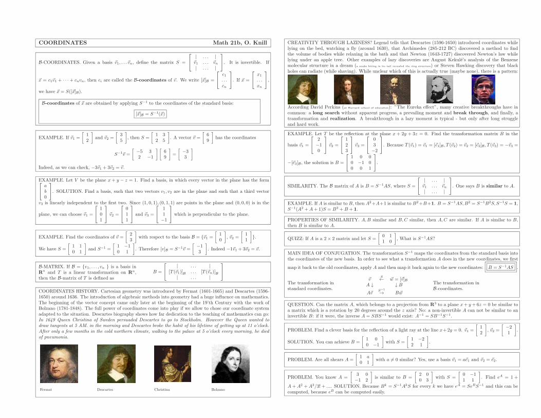
COORDINATES Math 21b, O. Knill

B-COORDINATES. Given a basis ~v1, . . . ~vn, define the matrix S =

| . . . |~v1 . . . ~vn| . . . |

. It is invertible. If

~x = c1~v1 + · · · + cnvn, then ci are called the B-coordinates of ~v. We write [~x]B =

c1. . .cn

. If ~x =

x1

. . .xn

,

we have ~x = S([~x]B).

B-coordinates of ~x are obtained by applying S−1 to the coordinates of the standard basis:

[~x]B = S−1(~x)

EXAMPLE. If ~v1 =

[

12

]

and ~v2 =

[

35

]

, then S =

[

1 32 5

]

. A vector ~v =

[

69

]

has the coordinates

S−1~v =

[

−5 32 −1

] [

69

]

=

[

−33

]

Indeed, as we can check, −3~v1 + 3~v2 = ~v.

EXAMPLE. Let V be the plane x + y − z = 1. Find a basis, in which every vector in the plane has the form

ab0

. SOLUTION. Find a basis, such that two vectors v1, v2 are in the plane and such that a third vector

v3 is linearly independent to the first two. Since (1, 0, 1), (0, 1, 1) are points in the plane and (0, 0, 0) is in the

plane, we can choose ~v1 =

101

~v2 =

011

and ~v3 =

11−1

which is perpendicular to the plane.

EXAMPLE. Find the coordinates of ~v =

[

23

]

with respect to the basis B = {~v1 =

[

10

]

, ~v2 =

[

11

]

}.

We have S =

[

1 10 1

]

and S−1 =

[

1 −10 1

]

. Therefore [v]B = S−1~v =

[

−13

]

. Indeed −1~v1 + 3~v2 = ~v.

B-MATRIX. If B = {v1, . . . , vn } is a basis inRn and T is a linear transformation on Rn,then the B-matrix of T is defined as

B =

| . . . |[T (~v1)]B . . . [T (~vn)]B| . . . |

COORDINATES HISTORY. Cartesian geometry was introduced by Fermat (1601-1665) and Descartes (1596-1650) around 1636. The introduction of algebraic methods into geometry had a huge influence on mathematics.The beginning of the vector concept came only later at the beginning of the 19’th Century with the work ofBolzano (1781-1848). The full power of coordinates come into play if we allow to chose our coordinate systemadapted to the situation. Descartes biography shows how far dedication to the teaching of mathematics can go:In 1649 Queen Christina of Sweden persuaded Descartes to go to Stockholm. However the Queen wanted to

draw tangents at 5 AM. in the morning and Descartes broke the habit of his lifetime of getting up at 11 o’clock.

After only a few months in the cold northern climate, walking to the palace at 5 o’clock every morning, he died

of pneumonia.

Fermat Descartes Christina Bolzano

CREATIVITY THROUGH LAZINESS? Legend tells that Descartes (1596-1650) introduced coordinates whilelying on the bed, watching a fly (around 1630), that Archimedes (285-212 BC) discovered a method to findthe volume of bodies while relaxing in the bath and that Newton (1643-1727) discovered Newton’s law whilelying under an apple tree. Other examples of lazy discoveries are August Kekule’s analysis of the Benzenemolecular structure in a dream (a snake biting in its tail revealed the ring structure) or Steven Hawking discovery that blackholes can radiate (while shaving). While unclear which of this is actually true (maybe none), there is a pattern:

According David Perkins (at Harvard school of education): ”The Eureka effect”, many creative breakthroughs have incommon: a long search without apparent progress, a prevailing moment and break through, and finally, atransformation and realization. A breakthrough in a lazy moment is typical - but only after long struggleand hard work.

EXAMPLE. Let T be the reflection at the plane x + 2y + 3z = 0. Find the transformation matrix B in the

basis ~v1 =

2−10

~v2 =

123

~v3 =

03−2

. Because T (~v1) = ~v1 = [~e1]B, T (~v2) = ~v2 = [~e2]B, T (~v3) = −~v3 =

−[~e3]B, the solution is B =

1 0 00 −1 00 0 1

.

SIMILARITY. The B matrix of A is B = S−1AS, where S =

| . . . |~v1 . . . ~vn| . . . |

. One says B is similar to A.

EXAMPLE. If A is similar to B, then A2+A+1 is similar to B2+B+1. B = S−1AS,B2 = S−1B2S, S−1S = 1,S−1(A2 +A+ 1)S = B2 +B + 1.

PROPERTIES OF SIMILARITY. A,B similar and B,C similar, then A,C are similar. If A is similar to B,then B is similar to A.

QUIZZ: If A is a 2× 2 matrix and let S =

[

0 11 0

]

, What is S−1AS?

MAIN IDEA OF CONJUGATION. The transformation S−1 maps the coordinates from the standard basis intothe coordinates of the new basis. In order to see what a transformation A does in the new coordinates, we first

map it back to the old coordinates, apply A and then map it back again to the new coordinates: B = S−1AS .

The transformation instandard coordinates.

~vS← ~w = [~v]B

A ↓ ↓ B

A~vS

−1

→ B~w

The transformation inB-coordinates.

QUESTION. Can the matrix A, which belongs to a projection from R3 to a plane x+ y+ 6z = 0 be similar toa matrix which is a rotation by 20 degrees around the z axis? No: a non-invertible A can not be similar to aninvertible B: if it were, the inverse A = SBS−1 would exist: A−1 = SB−1S−1.

PROBLEM. Find a clever basis for the reflection of a light ray at the line x+2y = 0. ~v1 =

[

12

]

, ~v2 =

[

−21

]

.

SOLUTION. You can achieve B =

[

1 00 −1

]

with S =

[

1 −22 1

]

.

PROBLEM. Are all shears A =

[

1 a0 1

]

with a 6= 0 similar? Yes, use a basis ~v1 = a~e1 and ~v2 = ~e2.

PROBLEM. You know A =

[

3 0−1 2

]

is similar to B =

[

2 00 3

]

with S =

[

0 −11 1

]

. Find eA = 1 +

A+ A2 + A3/3! + .... SOLUTION. Because Bk = S−1AkS for every k we have eA = SeBS−1 and this can becomputed, because eB can be computed easily.

FUNCTION SPACES Math 21b, O. Knill

FROM VECTORS TO FUNCTIONS AND MATRICES. Vectors can be displayed in different ways:

125326

1 2 3 4 5 6

1

2

3

4

5

6

1

2

3

4

56

1 2 3 4 5 6

1

2

3

4

5

6

The values (i, ~vi) can be interpreted as the graph of a function f : 1, 2, 3, 4, 5, 6→ R, where f(i) = ~vi.

Also matrices can be treated as functions, but as a function of two variables. If M is a 8×8 matrix for example,we get a function f(i, j) = [M ]ij which assigns to each square of the 8× 8 checkerboard a number.

LINEAR SPACES. A space X which contains 0, in which we can add, perform scalar multiplications and wherebasic laws like commutativity, distributivity and associativity hold, is called a linear space.

BASIC EXAMPLE. If A is a set, the space X of all functions from A to R is a linear space. Here are threeimportant special cases:

EUCLIDEAN SPACE: If A = {1, 2, 3, ..., n}, then X is Rn itself.FUNCTION SPACE: If A is the real line, then X is a the space of all functions in one variable.SPACE OF MATRICES: If A is the set

(1, 1) (1, 2) . . . (1,m)(2, 1) (2, 2) . . . (2,m). . . . . . . . . . . .

(n, 1) (n, 2) . . . (n,m) .

Then X is the space of all n×m matrices.

EXAMPLES.

• The n-dimensional space Rn.

• linear subspaces of Rn like the trivial space {0}, lines or planes etc.

• Mn, the space of all square n× n matrices.

• Pn, the space of all polynomials of degree n.

• The space P of all polynomials.

• C∞, the space of all smooth functions on the line

• C0, the space of all continuous functions on the line.

• C∞(R3, R3) the space of all smooth vector fields in three dimensional space.

• C1, the space of all differentiable functions on the line.

• C∞(R3) the space of all smooth functions in space.

• L2 the space of all functions for which∫∞

∞ f2(x) dx < ∞.

ZERO VECTOR. The function f which is everywhere equal to 0 is called the zero function. It plays the roleof the zero vector in Rn. If we add this function to an other function g we get 0 + g = g.

Careful, the roots of a function have nothing to do with the zero function. You should think of the roots of afunction like as zero entries of a vector. For the zero vector, all entries have to be zero. For the zero function,all values f(x) are zero.

CHECK: For subsets X of a function space, of for a ssubset of matrices Rn, we can check three properties tosee whether the space is a linear space:

i) if x, y are in X , then x+ y is in X .ii) If x is in X and λ is a real number, then λx is in X .iii) 0 is in X .

WHICH OF THE FOLLOWING ARE LINEAR SPACES?

The space X of all polynomials of degree exactly 4.

The space X of all continuous functions on the unit interval [−1, 1] which satisfy f(0) =1.

The space X of all smooth functions satisfying f(x + 1) = f(x). Example f(x) =sin(2πx) + cos(6πx).

The space X = sin(x) + C∞(R) of all smooth functions f(x) = sin(x) + g, where g is asmooth function.

The space X of all trigonometric polynomials f(x) = a0 + a1 sin(x) + a2 sin(2x) + ... +an sin(nx).

The spaceX of all smooth functions on R which satisfy f(1) = 1. It contains for examplef(x) = 1 + sin(x) + x.

The space X of all continuous functions on R which satisfy f(2) = 0 and f(10) = 0.

The space X of all smooth functions on R which satisfy lim|x|→∞ f(x) = 0.

The space X of all continuous functions on R which satisfy lim|x|→∞ f(x) = 1.

The space X of all smooth functions on R2.

The space X of all 2× 2 rotation dilation matrices

The space X of all upper triangular 3× 3 matrices.

The space X of all 2× 2 matrices A for which A11 = 1.

If you have seen multivariable calculus you can look at the following examples:

The space X of all vector fields (P,Q) in the plane, for which the curl Qx − Py is zeroeverywhere.

The space X of all vector fields (P,Q,R) in space, for which the divergence Px+Qy+Rz

is zero everywhere.

The space X of all vector fields (P,Q) in the plane for which the line integral∫

CF · dr

along the unit circle is zero.

The space X of all vector fields (P,Q,R) in space for which the flux through the unitsphere is zero.

The space X of all functions f(x, y) of two variables for which∫

1

0

∫

1

0f(x, y) dxdy = 0.

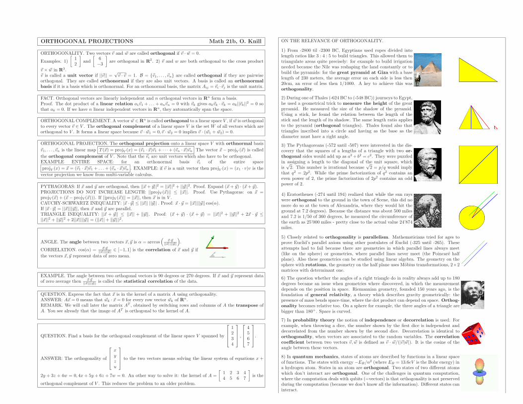
ORTHOGONAL PROJECTIONS Math 21b, O. Knill

ORTHOGONALITY. Two vectors ~v and ~w are called orthogonal if ~v · ~w = 0.

Examples. 1)

[

12

]

and

[

6−3

]

are orthogonal in R2. 2) ~v and w are both orthogonal to the cross product

~v × ~w in R3.~v is called a unit vector if ||~v|| =

√~v · ~v = 1. B = {~v1, . . . , ~vn} are called orthogonal if they are pairwise

orthogonal. They are called orthonormal if they are also unit vectors. A basis is called an orthonormal

basis if it is a basis which is orthonormal. For an orthonormal basis, the matrix Aij = ~vi ·~vj is the unit matrix.

FACT. Orthogonal vectors are linearly independent and n orthogonal vectors in Rn form a basis.Proof. The dot product of a linear relation a1~v1 + . . . + an~vn = 0 with ~vk gives ak~vk · ~vk = ak||~vk||2 = 0 sothat ak = 0. If we have n linear independent vectors in Rn, they automatically span the space.

ORTHOGONAL COMPLEMENT. A vector ~w ∈ Rn is called orthogonal to a linear space V , if ~w is orthogonalto every vector ~v ∈ V . The orthogonal complement of a linear space V is the set W of all vectors which areorthogonal to V . It forms a linear space because ~v · ~w1 = 0, ~v · ~w2 = 0 implies ~v · (~w1 + ~w2) = 0.

ORTHOGONAL PROJECTION. The orthogonal projection onto a linear space V with orthnormal basis

~v1, . . . , ~vn is the linear map T (~x) = projV (x) = (~v1 · ~x)~v1 + · · ·+ (~vn · ~x)~vn The vector ~x − projV (~x) is called

the orthogonal complement of V . Note that the ~vi are unit vectors which also have to be orthogonal.EXAMPLE ENTIRE SPACE: for an orthonormal basis ~vi of the entire space

projV (x) = ~x = (~v1 · ~x)~v1 + . . .+ (~vn · ~x)~vn . EXAMPLE: if ~v is a unit vector then projV (x) = (x1 · v)v is the

vector projection we know from multi-variable calculus.

PYTHAGORAS: If ~x and ~y are orthogonal, then ||~x+ ~y||2 = ||~x||2 + ||~y||2. Proof. Expand (~x+ ~y) · (~x+ ~y).PROJECTIONS DO NOT INCREASE LENGTH: ||projV(~x)|| ≤ ||~x||. Proof. Use Pythagoras: on ~x =projV(~x) + (~x− projV(~x))). If ||projV(~x)|| = ||~x||, then ~x is in V .CAUCHY-SCHWARTZ INEQUALITY: |~x · ~y| ≤ ||~x|| ||~y|| . Proof: ~x · ~y = ||~x||||~y|| cos(α).If |~x · ~y| = ||~x||||~y||, then ~x and ~y are parallel.TRIANGLE INEQUALITY: ||~x + ~y|| ≤ ||~x|| + ||~y||. Proof: (~x + ~y) · (~x + ~y) = ||~x||2 + ||~y||2 + 2~x · ~y ≤||~x||2 + ||~y||2 + 2||~x||||~y|| = (||~x||+ ||~y||)2.

ANGLE. The angle between two vectors ~x, ~y is α = arccos(

~x·~y||~x||||~y||

)

.

CORRELATION. cos(α) = ~x·~y||~x||||~y|| ∈ [−1, 1] is the correlation of ~x and ~y if

the vectors ~x, ~y represent data of zero mean.

EXAMPLE. The angle between two orthogonal vectors is 90 degrees or 270 degrees. If ~x and ~y represent dataof zero average then ~x·~y

||~x||||~y|| is called the statistical correlation of the data.

QUESTION. Express the fact that ~x is in the kernel of a matrix A using orthogonality.ANSWER: A~x = 0 means that ~wk · ~x = 0 for every row vector ~wk of Rn.REMARK. We will call later the matrix AT , obtained by switching rows and columns of A the transpose ofA. You see already that the image of AT is orthogonal to the kernel of A.

QUESTION. Find a basis for the orthogonal complement of the linear space V spanned by

1234

,

4567

.

ANSWER: The orthogonality of

xyzu

to the two vectors means solving the linear system of equations x +

2y + 3z + 4w = 0, 4x+ 5y + 6z + 7w = 0. An other way to solve it: the kernel of A =

[

1 2 3 44 5 6 7

]

is the

orthogonal complement of V . This reduces the problem to an older problem.

ON THE RELEVANCE OF ORTHOGONALITY.

1) From -2800 til -2300 BC, Egyptians used ropes divided intolength ratios like 3 : 4 : 5 to build triangles. This allowed them totriangulate areas quite precisely: for example to build irrigationneeded because the Nile was reshaping the land constantly or tobuild the pyramids: for the great pyramid at Giza with a baselength of 230 meters, the average error on each side is less then20cm, an error of less then 1/1000. A key to achieve this wasorthogonality.

2) During one of Thales (-624 BC to (-548 BC)) journeys to Egypt,he used a geometrical trick to measure the height of the greatpyramid. He measured the size of the shadow of the pyramid.Using a stick, he found the relation between the length of thestick and the length of its shadow. The same length ratio appliesto the pyramid (orthogonal triangles). Thales found also thattriangles inscribed into a circle and having as the base as thediameter must have a right angle.

3) The Pythagoreans (-572 until -507) were interested in the dis-covery that the squares of a lengths of a triangle with two or-

thogonal sides would add up as a2 + b2 = c2. They were puzzledin assigning a length to the diagonal of the unit square, whichis

√2. This number is irrational because

√2 = p/q would imply

that q2 = 2p2. While the prime factorization of q2 contains aneven power of 2, the prime factorization of 2p2 contains an oddpower of 2.

4) Eratosthenes (-274 until 194) realized that while the sun rayswere orthogonal to the ground in the town of Scene, this did nomore do so at the town of Alexandria, where they would hit theground at 7.2 degrees). Because the distance was about 500 milesand 7.2 is 1/50 of 360 degrees, he measured the circumference ofthe earth as 25’000 miles - pretty close to the actual value 24’874miles.

5) Closely related to orthogonality is parallelism. Mathematicians tried for ages toprove Euclid’s parallel axiom using other postulates of Euclid (-325 until -265). Theseattempts had to fail because there are geometries in which parallel lines always meet(like on the sphere) or geometries, where parallel lines never meet (the Poincare halfplane). Also these geometries can be studied using linear algebra. The geometry on thesphere with rotations, the geometry on the half plane uses Mobius transformations, 2×2matrices with determinant one.

6) The question whether the angles of a right triangle do in reality always add up to 180degrees became an issue when geometries where discovered, in which the measurementdepends on the position in space. Riemannian geometry, founded 150 years ago, is thefoundation of general relativity, a theory which describes gravity geometrically: thepresence of mass bends space-time, where the dot product can depend on space. Orthog-

onality becomes relative too. On a sphere for example, the three angles of a triangle arebigger than 180+. Space is curved.

7) In probability theory the notion of independence or decorrelation is used. Forexample, when throwing a dice, the number shown by the first dice is independent anddecorrelated from the number shown by the second dice. Decorrelation is identical toorthogonality, when vectors are associated to the random variables. The correlation

coefficient between two vectors ~v, ~w is defined as ~v · ~w/(|~v|~w|). It is the cosine of theangle between these vectors.

8) In quantum mechanics, states of atoms are described by functions in a linear spaceof functions. The states with energy −EB/n

2 (where EB = 13.6eV is the Bohr energy) ina hydrogen atom. States in an atom are orthogonal. Two states of two different atomswhich don’t interact are orthogonal. One of the challenges in quantum computation,where the computation deals with qubits (=vectors) is that orthogonality is not preservedduring the computation (because we don’t know all the information). Different states caninteract.

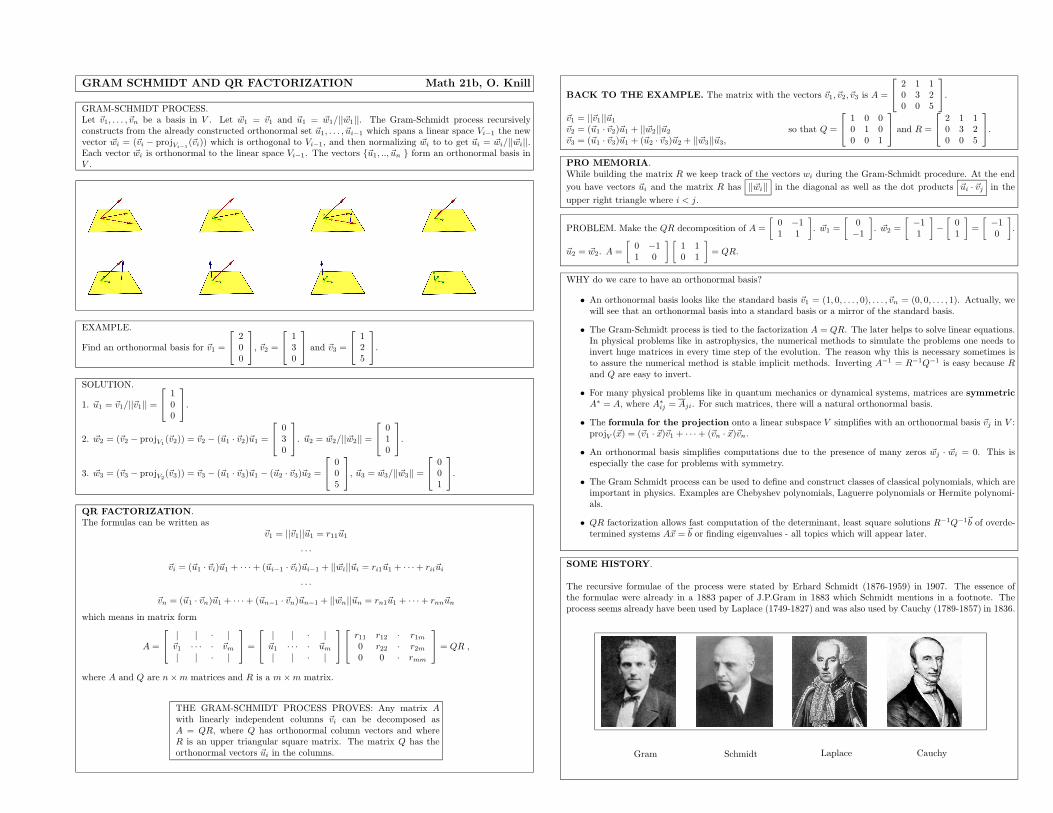
GRAM SCHMIDT AND QR FACTORIZATION Math 21b, O. Knill

GRAM-SCHMIDT PROCESS.Let ~v1, . . . , ~vn be a basis in V . Let ~w1 = ~v1 and ~u1 = ~w1/||~w1||. The Gram-Schmidt process recursivelyconstructs from the already constructed orthonormal set ~u1, . . . , ~ui−1 which spans a linear space Vi−1 the newvector ~wi = (~vi − projVi−1

(~vi)) which is orthogonal to Vi−1, and then normalizing ~wi to to get ~ui = ~wi/||~wi||.Each vector ~wi is orthonormal to the linear space Vi−1. The vectors {~u1, .., ~un } form an orthonormal basis inV .

EXAMPLE.

Find an orthonormal basis for ~v1 =

200

, ~v2 =

130

and ~v3 =

125

.

SOLUTION.

1. ~u1 = ~v1/||~v1|| =

100

.

2. ~w2 = (~v2 − projV1(~v2)) = ~v2 − (~u1 · ~v2)~u1 =

030

. ~u2 = ~w2/||~w2|| =

010

.

3. ~w3 = (~v3 − projV2(~v3)) = ~v3 − (~u1 · ~v3)~u1 − (~u2 · ~v3)~u2 =

005

, ~u3 = ~w3/||~w3|| =

001

.

QR FACTORIZATION.The formulas can be written as

~v1 = ||~v1||~u1 = r11~u1

· · ·

~vi = (~u1 · ~vi)~u1 + · · ·+ (~ui−1 · ~vi)~ui−1 + ||~wi||~ui = ri1~u1 + · · ·+ rii~ui

· · ·

~vn = (~u1 · ~vn)~u1 + · · ·+ (~un−1 · ~vn)~un−1 + ||~wn||~un = rn1~u1 + · · ·+ rnn~un

which means in matrix form

A =

| | · |~v1 · · · · ~vm| | · |

=

| | · |~u1 · · · · ~um

| | · |

r11 r12 · r1m0 r22 · r2m0 0 · rmm

= QR ,

where A and Q are n×m matrices and R is a m×m matrix.

THE GRAM-SCHMIDT PROCESS PROVES: Any matrix Awith linearly independent columns ~vi can be decomposed asA = QR, where Q has orthonormal column vectors and whereR is an upper triangular square matrix. The matrix Q has theorthonormal vectors ~ui in the columns.

BACK TO THE EXAMPLE. The matrix with the vectors ~v1, ~v2, ~v3 is A =

2 1 10 3 20 0 5

.

~v1 = ||~v1||~u1

~v2 = (~u1 · ~v2)~u1 + ||~w2||~u2

~v3 = (~u1 · ~v3)~u1 + (~u2 · ~v3)~u2 + ||~w3||~u3,so that Q =

1 0 00 1 00 0 1

and R =

2 1 10 3 20 0 5

.

PRO MEMORIA.While building the matrix R we keep track of the vectors wi during the Gram-Schmidt procedure. At the end

you have vectors ~ui and the matrix R has ||~wi|| in the diagonal as well as the dot products ~ui · ~vj in the

upper right triangle where i < j.

PROBLEM. Make the QR decomposition of A =

[

0 −11 1

]

. ~w1 =

[

0−1

]

. ~w2 =

[

−11

]

−

[

01

]

=

[

−10

]

.

~u2 = ~w2. A =

[

0 −11 0

] [

1 10 1

]

= QR.

WHY do we care to have an orthonormal basis?

• An orthonormal basis looks like the standard basis ~v1 = (1, 0, . . . , 0), . . . , ~vn = (0, 0, . . . , 1). Actually, wewill see that an orthonormal basis into a standard basis or a mirror of the standard basis.

• The Gram-Schmidt process is tied to the factorization A = QR. The later helps to solve linear equations.In physical problems like in astrophysics, the numerical methods to simulate the problems one needs toinvert huge matrices in every time step of the evolution. The reason why this is necessary sometimes isto assure the numerical method is stable implicit methods. Inverting A−1 = R−1Q−1 is easy because Rand Q are easy to invert.

• For many physical problems like in quantum mechanics or dynamical systems, matrices are symmetric

A∗ = A, where A∗

ij = Aji. For such matrices, there will a natural orthonormal basis.

• The formula for the projection onto a linear subspace V simplifies with an orthonormal basis ~vj in V :projV (~x) = (~v1 · ~x)~v1 + · · ·+ (~vn · ~x)~vn.

• An orthonormal basis simplifies computations due to the presence of many zeros ~wj · ~wi = 0. This isespecially the case for problems with symmetry.

• The Gram Schmidt process can be used to define and construct classes of classical polynomials, which areimportant in physics. Examples are Chebyshev polynomials, Laguerre polynomials or Hermite polynomi-als.

• QR factorization allows fast computation of the determinant, least square solutions R−1Q−1~b of overde-termined systems A~x = ~b or finding eigenvalues - all topics which will appear later.

SOME HISTORY.

The recursive formulae of the process were stated by Erhard Schmidt (1876-1959) in 1907. The essence ofthe formulae were already in a 1883 paper of J.P.Gram in 1883 which Schmidt mentions in a footnote. Theprocess seems already have been used by Laplace (1749-1827) and was also used by Cauchy (1789-1857) in 1836.

Gram Schmidt Laplace Cauchy

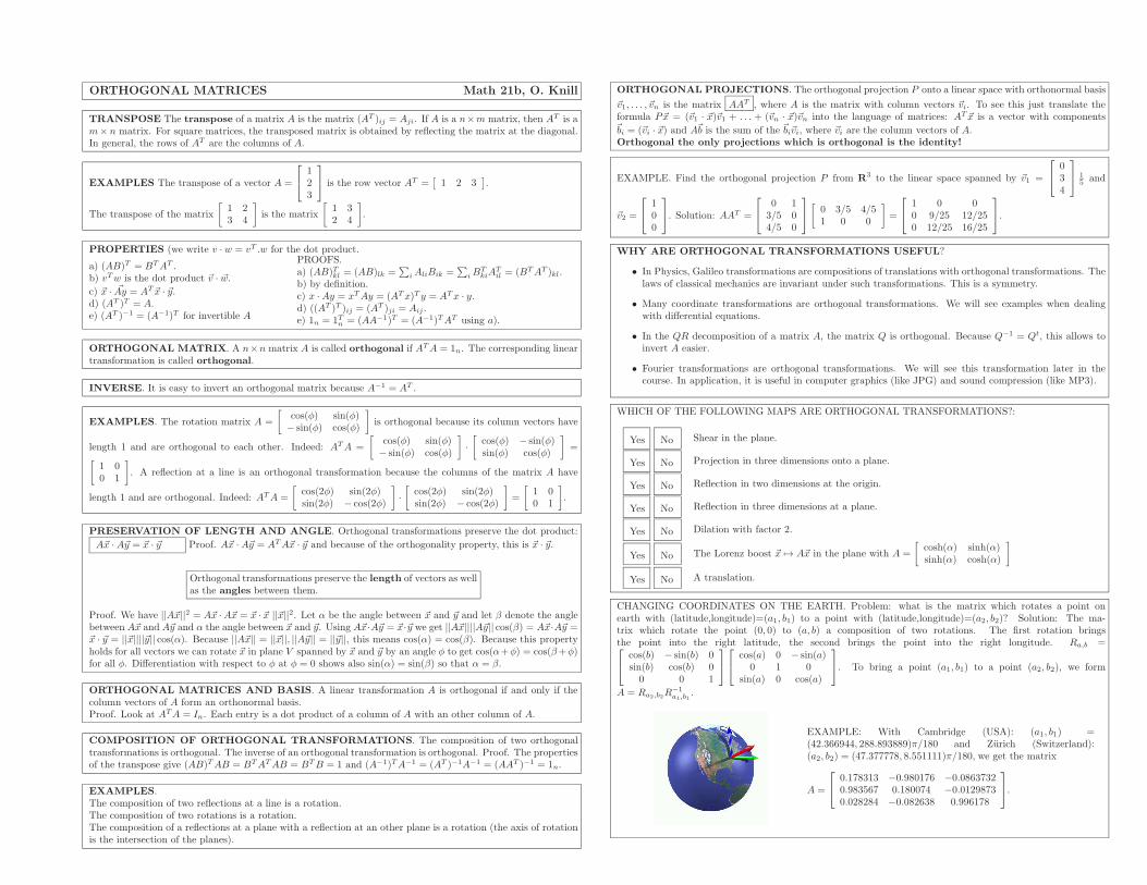
ORTHOGONAL MATRICES Math 21b, O. Knill

TRANSPOSE The transpose of a matrix A is the matrix (AT )ij = Aji. If A is a n×m matrix, then AT is am× n matrix. For square matrices, the transposed matrix is obtained by reflecting the matrix at the diagonal.In general, the rows of AT are the columns of A.

EXAMPLES The transpose of a vector A =

123

is the row vector AT =[

1 2 3]

.

The transpose of the matrix

[

1 23 4

]

is the matrix

[

1 32 4

]

.

PROPERTIES (we write v · w = vT .w for the dot product.

a) (AB)T = BTAT .b) vTw is the dot product ~v · ~w.

c) ~x · ~Ay = AT~x · ~y.d) (AT )T = A.e) (AT )−1 = (A−1)T for invertible A

PROOFS.a) (AB)Tkl = (AB)lk =

∑

iAliBik =∑

iBTkiA

Til = (BTAT )kl.

b) by definition.c) x ·Ay = xTAy = (ATx)T y = ATx · y.d) ((AT )T )ij = (AT )ji = Aij .e) 1n = 1Tn = (AA−1)T = (A−1)TAT using a).

ORTHOGONAL MATRIX. A n×n matrix A is called orthogonal if ATA = 1n. The corresponding lineartransformation is called orthogonal.

INVERSE. It is easy to invert an orthogonal matrix because A−1 = AT .

EXAMPLES. The rotation matrix A =

[

cos(φ) sin(φ)− sin(φ) cos(φ)

]

is orthogonal because its column vectors have

length 1 and are orthogonal to each other. Indeed: ATA =

[

cos(φ) sin(φ)− sin(φ) cos(φ)

]

·

[

cos(φ) − sin(φ)sin(φ) cos(φ)

]

=[

1 00 1

]

. A reflection at a line is an orthogonal transformation because the columns of the matrix A have

length 1 and are orthogonal. Indeed: ATA =

[

cos(2φ) sin(2φ)sin(2φ) − cos(2φ)

]

·

[

cos(2φ) sin(2φ)sin(2φ) − cos(2φ)

]

=

[

1 00 1

]

.

PRESERVATION OF LENGTH AND ANGLE. Orthogonal transformations preserve the dot product:

A~x · A~y = ~x · ~y Proof. A~x · A~y = ATA~x · ~y and because of the orthogonality property, this is ~x · ~y.

Orthogonal transformations preserve the length of vectors as wellas the angles between them.

Proof. We have ||A~x||2 = A~x ·A~x = ~x · ~x ||~x||2. Let α be the angle between ~x and ~y and let β denote the anglebetween A~x and A~y and α the angle between ~x and ~y. Using A~x·A~y = ~x·~y we get ||A~x||||A~y|| cos(β) = A~x·A~y =~x · ~y = ||~x||||~y|| cos(α). Because ||A~x|| = ||~x||, ||A~y|| = ||~y||, this means cos(α) = cos(β). Because this propertyholds for all vectors we can rotate ~x in plane V spanned by ~x and ~y by an angle φ to get cos(α+φ) = cos(β+φ)for all φ. Differentiation with respect to φ at φ = 0 shows also sin(α) = sin(β) so that α = β.

ORTHOGONAL MATRICES AND BASIS. A linear transformation A is orthogonal if and only if thecolumn vectors of A form an orthonormal basis.Proof. Look at ATA = In. Each entry is a dot product of a column of A with an other column of A.

COMPOSITION OF ORTHOGONAL TRANSFORMATIONS. The composition of two orthogonaltransformations is orthogonal. The inverse of an orthogonal transformation is orthogonal. Proof. The propertiesof the transpose give (AB)TAB = BTATAB = BTB = 1 and (A−1)TA−1 = (AT )−1A−1 = (AAT )−1 = 1n.

EXAMPLES.The composition of two reflections at a line is a rotation.The composition of two rotations is a rotation.The composition of a reflections at a plane with a reflection at an other plane is a rotation (the axis of rotationis the intersection of the planes).

ORTHOGONAL PROJECTIONS. The orthogonal projection P onto a linear space with orthonormal basis

~v1, . . . , ~vn is the matrix AAT , where A is the matrix with column vectors ~vi. To see this just translate theformula P~x = (~v1 · ~x)~v1 + . . . + (~vn · ~x)~vn into the language of matrices: AT~x is a vector with components~bi = (~vi · ~x) and A~b is the sum of the ~bi~vi, where ~vi are the column vectors of A.Orthogonal the only projections which is orthogonal is the identity!

EXAMPLE. Find the orthogonal projection P from R3 to the linear space spanned by ~v1 =

034

1

5and

~v2 =

100

. Solution: AAT =

0 13/5 04/5 0

[

0 3/5 4/51 0 0

]

=

1 0 00 9/25 12/250 12/25 16/25

.

WHY ARE ORTHOGONAL TRANSFORMATIONS USEFUL?

• In Physics, Galileo transformations are compositions of translations with orthogonal transformations. Thelaws of classical mechanics are invariant under such transformations. This is a symmetry.

• Many coordinate transformations are orthogonal transformations. We will see examples when dealingwith differential equations.

• In the QR decomposition of a matrix A, the matrix Q is orthogonal. Because Q−1 = Qt, this allows toinvert A easier.

• Fourier transformations are orthogonal transformations. We will see this transformation later in thecourse. In application, it is useful in computer graphics (like JPG) and sound compression (like MP3).

WHICH OF THE FOLLOWING MAPS ARE ORTHOGONAL TRANSFORMATIONS?:

Yes No Shear in the plane.

Yes No Projection in three dimensions onto a plane.

Yes No Reflection in two dimensions at the origin.

Yes No Reflection in three dimensions at a plane.

Yes No Dilation with factor 2.

Yes No The Lorenz boost ~x 7→ A~x in the plane with A =

[

cosh(α) sinh(α)sinh(α) cosh(α)

]

Yes No A translation.

CHANGING COORDINATES ON THE EARTH. Problem: what is the matrix which rotates a point onearth with (latitude,longitude)=(a1, b1) to a point with (latitude,longitude)=(a2, b2)? Solution: The ma-trix which rotate the point (0, 0) to (a, b) a composition of two rotations. The first rotation bringsthe point into the right latitude, the second brings the point into the right longitude. Ra,b =

cos(b) − sin(b) 0sin(b) cos(b) 00 0 1

cos(a) 0 − sin(a)0 1 0

sin(a) 0 cos(a)

. To bring a point (a1, b1) to a point (a2, b2), we form

A = Ra2,b2R−1

a1,b1.

EXAMPLE: With Cambridge (USA): (a1, b1) =(42.366944, 288.893889)π/180 and Zurich (Switzerland):(a2, b2) = (47.377778, 8.551111)π/180, we get the matrix

A =

0.178313 −0.980176 −0.08637320.983567 0.180074 −0.01298730.028284 −0.082638 0.996178

.

LEAST SQUARES AND DATA Math 21b, O. Knill

GOAL. The best possible ”solution” of an inconsistent linear systems Ax = b is called the least square

solution. It is the orthogonal projection of b onto the image im(A) of A. What we know about the kerneland the image of linear transformations helps to understand this situation and leads to an explicit formulasfor the least square fit. Why do we care about non-consistent systems? Often we have to solve linear systemsof equations with more constraints than variables. An example is when we try to find the best polynomialwhich passes through a set of points. This problem is called data fitting. If we wanted to accommodate alldata, the degree of the polynomial would become too large. The fit would look too wiggly. Taking a smallerdegree polynomial will not only be more convenient but also give a better picture. Especially important isregression, the fitting of data with lines.

The above pictures show 30 data points which are fitted best with polynomials of degree 1, 6, 11 and 16. Thefirst linear fit maybe tells most about the trend of the data.

THE ORTHOGONAL COMPLEMENT OF im(A). Because a vector is in the kernel of AT if and only ifit is orthogonal to the rows of AT and so to the columns of A, the kernel of AT is the orthogonal complement

of im(A): (im(A))⊥ = ker(AT )

EXAMPLES.

1) A =

abc

. The kernel V of AT =[

a b c]

consists of all vectors satisfying ax + by + cz = 0. V is a

plane. The orthogonal complement is the image of A which is spanned by the normal vector

abc

to the plane.

2) A =

[

1 10 0

]

. The image of A is spanned by

[

10

]

the kernel of AT is spanned by

[

01

]

.

ORTHOGONAL PROJECTION. If ~b is a vector and V is a linear subspace, then projV (~b) is the vector

closest to ~b on V : given any other vector ~v on V , one can form the triangle ~b, ~v, projV(~b) which has a right angle

at projV (~b) and invoke Pythagoras.

THE KERNEL OF ATA. For any m× n matrix ker(A) = ker(ATA) Proof. ⊂ is clear. On the other

hand ATAv = 0 means that Av is in the kernel of AT . But since the image of A is orthogonal to the kernel ofAT , we have A~v = 0, which means ~v is in the kernel of A.

LEAST SQUARE SOLUTION. The least square so-

lution of A~x = ~b is the vector ~x∗ such that A~x∗ isclosest to ~b from all other vectors A~x. In other words,A~x∗ = proj

V(~b), where V = im(V ). Because ~b − A~x∗

is in V ⊥ = im(A)⊥ = ker(AT ), we have AT (~b − A~x∗) =0. The last equation means that ~x∗ is a solution of

ATA~x = AT~b, the normal

equation of A~x = ~b. If the kernel of A is triv-

ial, then the kernel of ATA is trivial and ATA can be inverted.

Therefore ~x∗ = (ATA)−1AT~b is the least square solution.

V=im(A)

Tker(A )= im(A)

T b

Ax*

A (b-Ax)=0T

Ax=A(A A) A bT T-1*

WHY LEAST SQUARES? If ~x∗ is the least square solution of A~x = ~b then ||A~x∗ −~b|| ≤ ||A~x −~b|| for all ~x.Proof. AT (A~x∗ −~b) = 0 means that A~x∗ −~b is in the kernel of AT which is orthogonal to V = im(A). That is

projV(~b) = A~x∗ which is the closest point to ~b on V .

ORTHOGONAL PROJECTION If ~v1, . . . , ~vn is a basis in V which is not necessarily orthonormal, then

the orthogonal projection is ~x 7→ A(ATA)−1AT (~x) where A = [~v1, . . . , ~vn].

Proof. ~x = (ATA)−1AT~b is the least square solution of A~x = ~b. Therefore A~x = A(ATA)−1AT~b is the vector

in im(A) closest to ~b.

Special case: If ~w1, . . . , ~wn is an orthonormal basis in V , we had seen earlier that AAT with A = [~w1, . . . , ~wn]is the orthogonal projection onto V (this was just rewriting A~x = (~w1 · ~x)~w1 + · · ·+(~wn · ~x)~wn in matrix form.)This follows from the above formula because ATA = I in that case.

EXAMPLE Let A =

1 02 00 1

. The orthogonal projection onto V = im(A) is ~b 7→ A(ATA)−1AT~b. We have

ATA =

[

5 02 1

]

and A(ATA)−1AT =

1/5 2/5 02/5 4/5 00 0 1

.

For example, the projection of ~b =

010

is ~x∗ =

2/54/50

and the distance to ~b is 1/√5. The point ~x∗ is the

point on V which is closest to ~b.

Remember the formula for the distance of ~b to a plane V with normal vector ~n? It was d = |~n · ~b|/||~n||.In our case, we can take ~n = [−2, 1, 0] and get the distance 1/

√5. Let’s check: the distance of ~x∗ and ~b is

||(2/5,−1/5, 0)|| = 1/√5.

EXAMPLE. Let A =

1201

. Problem: find the matrix of the orthogonal projection onto the image of A.

The image of A is a one-dimensional line spanned by the vector ~v = (1, 2, 0, 1). We calculate ATA = 6. Then

A(ATA)−1AT =

1201

[

1 2 0 1]

/6 =

1 2 0 12 4 0 20 0 0 01 2 0 1

/6

DATA FIT. Find a quadratic polynomial p(t) = at2 + bt + c which best fits the four data points(−1, 8), (0, 8), (1, 4), (2, 16).

A =

1 −1 10 0 11 1 14 2 1

~b =

88416

T

. ATA =

18 8 68 6 26 2 4

and ~x∗ = (ATA)−1AT~b =

3−15

.

Software packages like Mathematica have alreadybuilt in the facility to fit numerical data:

The series expansion of f showed that indeed, f(t) = 5 − t + 3t2 is indeed best quadratic fit. Actually,Mathematica does the same to find the fit then what we do: ”Solving” an inconsistent system of linear

equations as best as possible.

PROBLEM: Prove im(A) = im(AAT ).

SOLUTION. The image of AAT is contained in the image of A because we can write ~v = AAT ~x as ~v = A~y with~y = AT ~x. On the other hand, if ~v is in the image of A, then ~v = A~x. If ~x = ~y + ~z, where ~y in the kernel ofA and ~z orthogonal to the kernel of A, then A~x = A~z. Because ~z is orthogonal to the kernel of A, it is in theimage of AT . Therefore, ~z = AT ~u and ~v = A~z = AAT~u is in the image of AAT .

DETERMINANTS I Math 21b, O. Knill

PERMUTATIONS. A permutation of {1, 2, . . . , n} is a rearrangementof {1, 2, . . . , n}. There are n! = n · (n − 1)... · 1 different permutationsof {1, 2, . . . , n}: fixing the position of first element leaves (n − 1)!possibilities to permute the rest.

EXAMPLE. There are 6 permutations of {1, 2, 3}:(1, 2, 3), (1, 3, 2), (2, 1, 3), (2, 3, 1), (3, 1, 2), (3, 2, 1).

PATTERNS AND SIGN. The matrix A with zeros everywhere exceptat the positions Ai,π(i) = 1 forming a pattern of π. An up-crossing

is a pair k < l such that π(k) < π(l). The sign of a permutation π isdefined as sign(π) = (−1)u where u is the number of up-crossings in thepattern of π. It is the number pairs of black squares, where the uppersquare is to the right.

EXAMPLES. sign(1, 2) = 0, sign(2, 1) = 1. sign(1, 2, 3) = sign(3, 2, 1) =sign(2, 3, 1) = 1. sign(1, 3, 2) = sign(3, 2, 1) = sign(2, 1, 3) = −1.

DETERMINANT The determinant of a n× n matrix A = aij is defined as the sum

∑

π sign(π)a1π(1)a2π(2) · · · anπ(n)

where π is a permutation of {1, 2, . . . , n}.

2 × 2 CASE. The determinant of A =

∣

∣

∣

∣

a bc d

∣

∣

∣

∣

is ad − bc. There are two permutations of (1, 2). The identity

permutation (1, 2) gives a11a12, the permutation (2, 1) gives a21a22.If you have seen some multi-variable calculus, you know that det(A) is the area of the parallelogram spannedby the column vectors of A. The two vectors form a basis if and only if det(A) 6= 0.

3 × 3 CASE. The determinant of A =

∣

∣

∣

∣

∣

∣

a b cd e fg h i

∣

∣

∣

∣

∣

∣

is aei + bfg + cdh − ceg − fha− bdi corresponding to the

6 permutations of (1, 2, 3). Geometrically, det(A) is the volume of the parallelepiped spanned by the columnvectors of A. The three vectors form a basis if and only if det(A) 6= 0.

EXAMPLE DIAGONAL AND TRIANGULARMATRICES. The determinant of a diagonal or triangular matrixis the product of the diagonal elements.

EXAMPLE PERMUTATION MATRICES. The determinant of a matrix which has everywhere zeros exceptaiπ(j) = 1 is just the sign sign(π) of the permutation.

THE LAPLACE EXPANSION. To compute the determinant of a n× n matrices A = aij . Choose a column i.For each entry aji in that column, take the (n− 1)× (n− 1) matrix aij which does not contain the i’th columnand j’th row. The determinant of Aij is called a minor. One gets

det(A) = (−1)i+1ai1det(Ai1) + · · ·+ (−1)i+naindet(Ain) =∑n

j=1(−1)i+jaijdet(Aij)

This Laplace expansion is just a convenient arrangement of the permutations: listing all permutations of theform (1, ∗, ..., ∗) of n elements is the same then listing all permutations of (2, ∗, ..., ∗) of (n− 1) elements etc.

TRIANGULAR AND DIAGONAL MATRICES.The determinant of a diagonal or triangular

matrix is the product of its diagonal elements.

Example: det(

1 0 0 04 5 0 02 3 4 01 1 2 1

) = 20.

PARTITIONED MATRICES.The determinant of a partitioned matrix[

A 00 B

]

is the product det(A)det(B).

Example det(

3 4 0 01 2 0 00 0 4 −20 0 2 2

) = 2 · 12 = 24.

LINEARITY OF THE DETERMINANT. If the columns of A and B are the same except for the i’th column,

det([v1, ..., v, ...vn]] + det([v1, ..., w, ...vn]] = det([v1, ..., v + w, ...vn]]

In general, one has det([v1, ..., kv, ...vn]] = k det([v1, ..., v, ...vn]] The same identities hold for rows and follow

directly from the original definition of the determimant.

ROW REDUCED ECHELON FORM. Determining rref(A) also determines det(A).If A is a matrix and λ1, ..., λk are the factors which are used to scale different rows and s is the total number

of times, two rows were switched, then det(A) = (−1)sα1 · · ·λk det(rref(A)) .

INVERTIBILITY. Because of the last formula: A n× n matrix A is invertible if and only if det(A) 6= 0.

PROBLEM. Find the determi-

nant of A =

0 0 0 21 2 4 50 7 2 90 0 6 4

.SOLUTION. Three row transpositions give B =

1 2 4 50 7 2 90 0 6 40 0 0 2

a ma-

trix which has determinant 84. Therefore det(A) = (−1)3det(B) = −84.

PROPERTIES OF DETERMINANTS. (combined with next lecture)

det(AB) = det(A)det(B)

det(A−1) = det(A)−1

det(SAS−1) = det(A)

det(AT ) = det(A)

det(λA) = λndet(A)

det(−A) = (−1)ndet(A)

If B is obtained from A by switching two rows, then det(B) = −det(A). If B is obtained by adding an otherrow to a given row, then this does not change the value of the determinant.

PROOF OF det(AB) = det(A)det(B), one brings the n × n matrix [A|AB] into row reduced echelon form.Similar than the augmented matrix [A|b] was brought into the form [1|A−1b], we end up with [1|A−1AB] = [1|B].By looking at the n× n matrix to the left during Gauss-Jordan elimination, the determinant has changed by afactor det(A). We end up with a matrix B which has determinant det(B). Therefore, det(AB) = det(A)det(B).PROOF OF det(AT ) = det(A). The transpose of a pattern is a pattern with the same signature.

PROBLEM. Determine det(A100), where A is the matrix

∣

∣

∣

∣

1 23 16

∣

∣

∣

∣

.

SOLUTION. det(A) = 10, det(A100) = (det(A))100 = 10100 = 1 · gogool. This name as well as the gogoolplex =

1010100

are official. They are huge numbers: the mass of the universe for example is 1052kg and 1/101051

is thechance to find yourself on Mars by quantum fluctuations. (R.E. Crandall, Scientific American, Feb. 1997).

ORTHOGONAL MATRICES. Because QTQ = 1, we have det(Q)2 = 1 and so |det(Q)| = 1 Rotations havedeterminant 1, reflections can have determinant −1.

QR DECOMPOSITION. If A = QR, then det(A) = det(Q)det(R). The determinant ofQ is±1, the determinantof R is the product of the diagonal elements of R.

HOW FAST CAN WE COMPUTE THE DETERMINANT?.

The cost to find the determinant is the same as for the Gauss-Jordanelimination. A measurements of the time needed for Mathematica tocompute a determinant of a random n × n matrix. The matrix sizeranged from n=1 to n=300. We see a cubic fit of these data.

WHY DO WE CARE ABOUT DETERMINANTS?

• check invertibility of matrices

• geometric interpretation as volume

• explicit algebraic inversion of a matrix

• is a natural functional on matrices (particle andstatistical physics)

• define orientation in any dimensions

• change of variable formulas in higher dimensions

• alternative concepts are unnatural

• check for similarity of matrices

DETERMINANTS II Math 21b, O.Knill

DETERMINANT AND VOLUME. If A is a n × n matrix, then |det(A)| is the volume of the n-dimensionalparallelepiped En spanned by the n column vectors vj of A.

Proof. Use the QR decomposition A = QR, where Q is orthogonal and R isupper triangular. From QQT = 1n, we get 1 = det(Q)det(QT ) = det(Q)2 see that|det(Q)| = 1. Therefore, det(A) = ±det(R). The determinant of R is the productof the ||ui|| = ||vi − projVj−1

vi|| which was the distance from vi to Vj−1. Thevolume vol(Ej) of a j-dimensional parallelepiped Ej with base Ej−1 in Vj−1 andheight ||ui|| is vol(Ej−1)||uj ||. Inductively vol(Ej) = ||uj ||vol(Ej−1) and thereforevol(En) =

∏n

j=1||uj || = det(R).

The volume of a k dimensional parallelepiped defined by the vectors v1, . . . , vk is√

det(ATA).

Proof. QTQ = In gives ATA = (QR)T (QR) = RTQTQR = RTR. So, det(RTR) = det(R)2 = (∏k

j=1||uj ||)

2.

(Note that A is a n× k matrix and that ATA = RTR and R are k × k matrices.)

ORIENTATION. Determinants allow to define the orientation of n vectors in n-dimensional space. This is”handy” because there is no ”right hand rule” in hyperspace ... To do so, define the matrix A with columnvectors vj and define the orientation as the sign of det(A). In three dimensions, this agrees with the right handrule: if v1 is the thumb, v2 is the pointing finger and v3 is the middle finger, then their orientation is positive.

b

i

det

x det(A) = iCRAMER’S RULE. This is an explicit formula for the solution of A~x = ~b. If Ai

denotes the matrix, where the column ~vi of A is replaced by ~b, then

xi = det(Ai)/det(A)

Proof. det(Ai) = det([v1, . . . , b, . . . , vn] = det([v1, . . . , (Ax), . . . , vn] =det([v1, . . . ,

∑

i xivi, . . . , vn] = xidet([v1, . . . , vi, . . . , vn]) = xidet(A)

EXAMPLE. Solve the system 5x+3y = 8, 8x+5y = 2 using Cramers rule. This linear system with A =

[

5 38 5

]

and b =

[

82

]

. We get x = det

[

8 32 5

]

= 34y = det

[

5 88 2

]

= −54.

GABRIEL CRAMER. (1704-1752), born in Geneva, Switzerland, he worked on geometryand analysis. Cramer used the rule named after him in a book ”Introduction a l’analysedes lignes courbes algebraique”, where he solved like this a system of equations with 5unknowns. According to a short biography of Cramer by J.J O’Connor and E F Robertson,the rule had however been used already before by other mathematicians. Solving systemswith Cramer’s formulas is slower than by Gaussian elimination. The rule is still important.For example, if A or b depends on a parameter t, and we want to see how x depends onthe parameter t one can find explicit formulas for (d/dt)xi(t).

THE INVERSE OF A MATRIX. Because the columns of A−1 are solutions of A~x = ~ei, where ~ej are basisvectors, Cramers rule together with the Laplace expansion gives the formula:

[A−1]ij = (−1)i+jdet(Aji)/det(A)

Bij = (−1)i+jdet(Aji) is called the classical adjoint or adjugate of A. Note the change ij → ji. Don’t

confuse the classical adjoint with the transpose AT which is sometimes also called the adjoint.

EXAMPLE. A =

2 3 15 2 46 0 7

has det(A) = −17 and we get A−1 =

14 −21 10−11 8 −3−12 18 −11

/(−17):

B11 = (−1)1+1det

[

2 40 7

]

= 14. B12 = (−1)1+2det

[

3 10 7

]

= −21. B13 = (−1)1+3det

[

3 12 4

]

= 10.

B21 = (−1)2+1det

[

5 46 7

]

= −11. B22 = (−1)2+2det

[

2 16 7

]

= 8. B23 = (−1)2+3det

[

2 15 4

]

= −3.

B31 = (−1)3+1det

[

5 26 0

]

= −12. B32 = (−1)3+2det

[

2 36 0

]

= 18. B33 = (−1)3+3det

[

2 35 2

]

= −11.

THE ART OF CALCULATING DETERMINANTS. When confronted with a matrix, it is good to go througha checklist of methods to crack the determinant. Often, there are different possibilities to solve the problem, inmany cases the solution is particularly simple using one method.

• Is it a upper or lower triangular matrix?

• Is it a partitioned matrix?

• Is it a product like det(A1000) = det(A)1000?

• Is the matrix known to be non invertible and sodet(A) = 0?

• Do you see duplicated columns or rows?

• Can you row reduce to a triangular case?

• Are there only a few nonzero patters?

• Try Laplace expansion with some row or column?

• Later: can we compute the eigenvalues of A?

EXAMPLES.

1) A =

1 2 3 4 52 4 6 8 105 5 5 5 41 3 2 7 43 2 8 4 9

Try row reduction. 2) A =

2 1 0 0 01 1 1 0 00 0 2 1 00 0 0 3 10 0 0 0 4

Laplace expansion.

3) A =

1 1 0 0 01 2 2 0 00 1 1 0 00 0 0 1 30 0 0 4 2

Partitioned matrix. 4) A =

1 6 10 1 152 8 17 1 290 0 3 8 120 0 0 4 90 0 0 0 5

Make it triangular.

APPLICATION HOFSTADTER BUTTERFLY. In solid state physics, one is interested in the function f(E) =det(L− EIn), where

L =

λ cos(α) 1 0 · 0 11 λ cos(2α) 1 · · 00 1 · · · ·· · · · 1 00 · · 1 λ cos((n− 1)α) 11 0 · 0 1 λ cos(nα)

describes an electron in a periodic crystal, E is the energy and α = 2π/n. The electron can move as a Blochwave whenever the determinant is negative. These intervals form the spectrum of the quantum mechanicalsystem. A physicist is interested in the rate of change of f(E) or its dependence on λ when E is fixed. .

-4 -2 2 4

1

2

3

4

5

6

The graph to the left shows the function E 7→log(|det(L − EIn)|) in the case λ = 2 and n = 5.In the energy intervals, where this function is zero,the electron can move, otherwise the crystal is an in-sulator. The picture to the right shows the spectrumof the crystal depending on α. It is called the ”Hofs-tadter butterfly” made popular in the book ”Godel,Escher Bach” by Douglas Hofstadter.

EIGENVALUES & DYNAMICAL SYSTEMS 21b,O.Knill

EIGENVALUES AND EIGENVECTORS. A nonzero vector v is called an eigenvector of a n × n matrix A

with eigenvalue λ if Av = λv .

EXAMPLES.

• ~v is an eigenvector to the eigenvalue 0 if ~v is inthe kernel of A.

• A rotation in space has an eigenvalue 1, witheigenvector spanning the axes of rotation.

• If A is a diagonal matrix with diagonal elementsai, then ~ei is an eigenvector with eigenvalue ai.

• A shear A in the direction v has an eigenvector~v.

• Projections have eigenvalues 1 or 0.

• Reflections have eigenvalues 1 or −1.

• A rotation in the plane by an angle 30 degreeshas no real eigenvector. (the eigenvectors are

complex).

LINEAR DYNAMICAL SYSTEMS.When applying a linear map x 7→ Ax again and again, obtain a discrete dynamical system. We want tounderstand what happens with the orbit x1 = Ax, x2 = AAx = A2x, x3 = AAAx = A3x, ....

EXAMPLE 1: x 7→ ax or xn+1 = axn has the solution xn = anx0. For example, 1.0320 · 1000 = 1806.11 isthe balance on a bank account which had 1000 dollars 20 years ago and if the interest rate was constant 3 percent.

EXAMPLE 2: A =

[

1 20 1

]

. ~v =

[

11

]

. A~v =

[

31

]

, A2~v =

[

51

]

. A3~v =

[

71

]

. A4~v =

[

91

]

etc.

EXAMPLE 3: If ~v is an eigenvector with eigenvalue λ, then A~v = λ~v,A2~v = A(A~v)) = Aλ~v = λA~v = λ2~v andmore generally An~v = λn~v.

RECURSION: If a scalar quantity un+1 does not only depend on un but also on un−1 we can write (xn, yn) =(un, un−1) and get a linear map because xn+1, yn+1 depend in a linear way on xn, yn.

EXAMPLE: Lets look at the recursionun+1 = un − un−1 with u0 = 0, u1 = 1.

Because

[

1 −11 0

] [

un

un−1

]

=

[

un+1

un

]

.

The recursion is done by iterating the ma-

trix A: A =

[

1 −11 0

]

A2 =

[

0 −11 −1

]

A3 =

[

−1 00 −1

]

. We see that A6 is the

identity. Every initial vector is mapped after6 iterations back to its original starting point.

If the E parameter is changed, the dynamicsalso changes. For E = 3 for example, mostinitial points will escape to infinity similar asin the next example. Indeed, for E = 3, thereis an eigenvector ~v = (3+

√5)/2 to the eigen-

value λ = (3 +√5)/2 and An~v = λn~v escapes

to ∞.

THE FIBONACCI RECURSION:

In the third section of Liber abbaci, published in1202, the mathematician Fibonacci, with real nameLeonardo di Pisa (1170-1250) writes:

”A certain man put a pair

of rabbits in a place sur-

rounded on all sides by a

wall. How many pairs

of rabbits can be produced

from that pair in a year

if it is supposed that ev-

ery month each pair begets

a new pair which from the

second month on becomes

productive?”

Mathematically, how does un grow, ifun+1 = un + un−1? We can assume u0 = 1 andu1 = 2 to match Leonardo’s example. The sequenceis (1, 2, 3, 5, 8, 13, 21, ...). As before we can writethis recursion using vectors (xn, yn) = (un, un−1)starting with (1, 2). The matrix A to this recursion

is A =

[

1 11 0

]

. Iterating gives A

[

21

]

=

[

32

]

,

A2

[

21

]

= A

[

32

]

=

[

53

]

.

ASSUME WE KNOW THE EIGENVALUES AND VECTORS: If A~v1 = λ1~v1, A~v2 = λ2~v2 and ~v = c1~v1+c2~v2,we have an explicit solution An~v = c1λ

n

1~v1+c2λn

2~v2. This motivates to find good methods to compute eigenvaluesand eigenvectors.

EVOLUTION OF QUANTITIES: Market systems, population quantities of different species, or ingredientquantities in a chemical reaction. A linear description might not always be be a good model but it has theadvantage that we can solve the system explicitly. Eigenvectors will provide the key to do so.

MARKOV MATRICES. A matrix with nonzero entries for which the sum of the columns entries add up to 1 iscalled a Markov matrix.

Markov Matrices have an eigenvalue 1.

Proof. The eigenvalues of A and AT are the same because they have the same characteristic polynomial. Thematrix AT has an eigenvector [1, 1, 1, 1, 1]T . An example is the matrix

A =

1/2 1/3 1/41/4 1/3 1/31/4 1/3 5/12

MARKOV PROCESS EXAMPLE: The percentage of people using Ap-

ple OS or the Linux OS is represented by a vector

[

ml

]

. Each cycle

2/3 of Mac OS users switch to Linux and 1/3 stays. Also lets assumethat 1/2 of the Linux OS users switch to apple and 1/2 stay. The matrix

P =

[

1/3 1/22/3 1/2

]

is a Markov matrix. What ratio of Apple/Linux

users do we have after things settle to an equilibrium? We can simulatethis with a dice: start in a state like M = (1, 0) (all users have Macs).If the dice shows 3,4,5 or 6, a user in that group switch to Linux, oth-erwise stays in the M camp. Throw also a dice for each user in L. If 1,2or 3 shows up, the user switches to M. The matrix P has an eigenvec-tor (3/7, 4/7) which belongs to the eigenvalue 1. The interpretation ofP~v = ~v is that with this split up, there is no change in average.

1

2

1

2

1

2

1

2

1

2

1

2

1 2

1

2

1

2

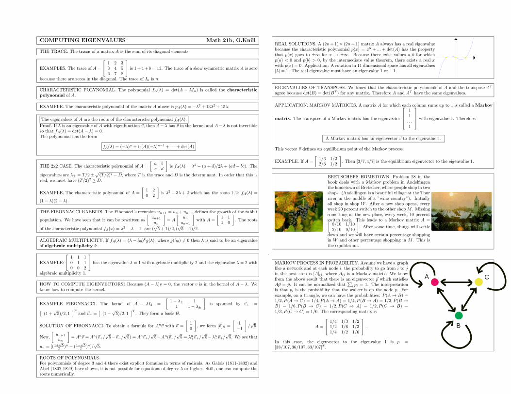
COMPUTING EIGENVALUES Math 21b, O.Knill

THE TRACE. The trace of a matrix A is the sum of its diagonal elements.

EXAMPLES. The trace of A =

1 2 33 4 56 7 8

is 1+4+8 = 13. The trace of a skew symmetric matrix A is zero

because there are zeros in the diagonal. The trace of In is n.

CHARACTERISTIC POLYNOMIAL. The polynomial fA(λ) = det(A − λIn) is called the characteristic

polynomial of A.

EXAMPLE. The characteristic polynomial of the matrix A above is pA(λ) = −λ3 + 13λ2 + 15λ.

The eigenvalues of A are the roots of the characteristic polynomial fA(λ).

Proof. If λ is an eigenvalue of A with eigenfunction ~v, then A−λ has ~v in the kernel and A−λ is not invertibleso that fA(λ) = det(A− λ) = 0.The polynomial has the form

fA(λ) = (−λ)n + tr(A)(−λ)n−1 + · · ·+ det(A)

THE 2x2 CASE. The characteristic polynomial of A =

[

a bc d

]

is fA(λ) = λ2 − (a + d)/2λ + (ad− bc). The

eigenvalues are λ± = T/2±√

(T/2)2 −D, where T is the trace and D is the determinant. In order that this isreal, we must have (T/2)2 ≥ D.

EXAMPLE. The characteristic polynomial of A =

[

1 20 2

]

is λ2 − 3λ + 2 which has the roots 1, 2: fA(λ) =

(1− λ)(2 − λ).

THE FIBONNACCI RABBITS. The Fibonacci’s recursion un+1 = un + un−1 defines the growth of the rabbit

population. We have seen that it can be rewritten as

[

un+1

un

]

= A

[

un

un−1

]

with A =

[

1 11 0

]

. The roots

of the characteristic polynomial fA(x) = λ2 − λ− 1. are (√5 + 1)/2, (

√5− 1)/2.

ALGEBRAIC MULTIPLICITY. If fA(λ) = (λ − λ0)kg(λ), where g(λ0) 6= 0 then λ is said to be an eigenvalue

of algebraic multiplicity k.

EXAMPLE:

1 1 10 1 10 0 2

has the eigenvalue λ = 1 with algebraic multiplicity 2 and the eigenvalue λ = 2 with

algebraic multiplicity 1.

HOW TO COMPUTE EIGENVECTORS? Because (A − λ)v = 0, the vector v is in the kernel of A − λ. Weknow how to compute the kernel.

EXAMPLE FIBONNACCI. The kernel of A − λI2 =

[

1− λ± 11 1− λ±

]

is spanned by ~v+ =

[

(1 +√5)/2, 1

]Tand ~v− =

[

(1 −√5)/2, 1

]T. They form a basis B.

SOLUTION OF FIBONNACCI. To obtain a formula for An~v with ~v =

[

10

]

, we form [~v]B =

[

1−1

]

/√5.

Now,

[

un+1

un

]

= An~v = An(~v+/√5−~v−/

√5) = An~v+/

√5−An(~v−/

√5 = λn

+~v+/√5−λn

−~v+/√5. We see that

un = [(1+√5

2)n − (1−

√5

2)n]/

√5.

ROOTS OF POLYNOMIALS.For polynomials of degree 3 and 4 there exist explicit formulas in terms of radicals. As Galois (1811-1832) andAbel (1802-1829) have shown, it is not possible for equations of degree 5 or higher. Still, one can compute theroots numerically.

REAL SOLUTIONS. A (2n+1)× (2n+1) matrix A always has a real eigenvaluebecause the characteristic polynomial p(x) = x5 + ... + det(A) has the propertythat p(x) goes to ±∞ for x → ±∞. Because there exist values a, b for whichp(a) < 0 and p(b) > 0, by the intermediate value theorem, there exists a real xwith p(x) = 0. Application: A rotation in 11 dimensional space has all eigenvalues|λ| = 1. The real eigenvalue must have an eigenvalue 1 or −1.

EIGENVALUES OF TRANSPOSE. We know that the characteristic polynomials of A and the transpose AT

agree because det(B) = det(BT ) for any matrix. Therefore A and AT have the same eigenvalues.

APPLICATION: MARKOV MATRICES. A matrix A for which each column sums up to 1 is called a Markov

matrix. The transpose of a Markov matrix has the eigenvector

11. . .1

with eigenvalue 1. Therefore:

A Markov matrix has an eigenvector ~v to the eigenvalue 1.

This vector ~v defines an equilibrium point of the Markov process.

EXAMPLE. If A =

[

1/3 1/22/3 1/2

]

. Then [3/7, 4/7] is the equilibrium eigenvector to the eigenvalue 1.

BRETSCHERS HOMETOWN. Problem 28 in thebook deals with a Markov problem in Andelfingenthe hometown of Bretscher, where people shop in twoshops. (Andelfingen is a beautiful village at the Thurriver in the middle of a ”wine country”). Initiallyall shop in shop W . After a new shop opens, everyweek 20 percent switch to the other shop M . Missingsomething at the new place, every week, 10 percentswitch back. This leads to a Markov matrix A =[

8/10 1/102/10 9/10

]

. After some time, things will settle

down and we will have certain percentage shoppingin W and other percentage shopping in M . This isthe equilibrium.

.

MARKOV PROCESS IN PROBABILITY. Assume we have a graphlike a network and at each node i, the probability to go from i to jin the next step is [A]ij , where Aij is a Markov matrix. We knowfrom the above result that there is an eigenvector ~p which satisfiesA~p = ~p. It can be normalized that

∑

i pi = 1. The interpretationis that pi is the probability that the walker is on the node p. Forexample, on a triangle, we can have the probabilities: P (A → B) =1/2, P (A → C) = 1/4, P (A → A) = 1/4, P (B → A) = 1/3, P (B →B) = 1/6, P (B → C) = 1/2, P (C → A) = 1/2, P (C → B) =1/3, P (C → C) = 1/6. The corresponding matrix is

A =

1/4 1/3 1/21/2 1/6 1/31/4 1/2 1/6

.

In this case, the eigenvector to the eigenvalue 1 is p =[38/107, 36/107, 33/107]T.

A

B

C

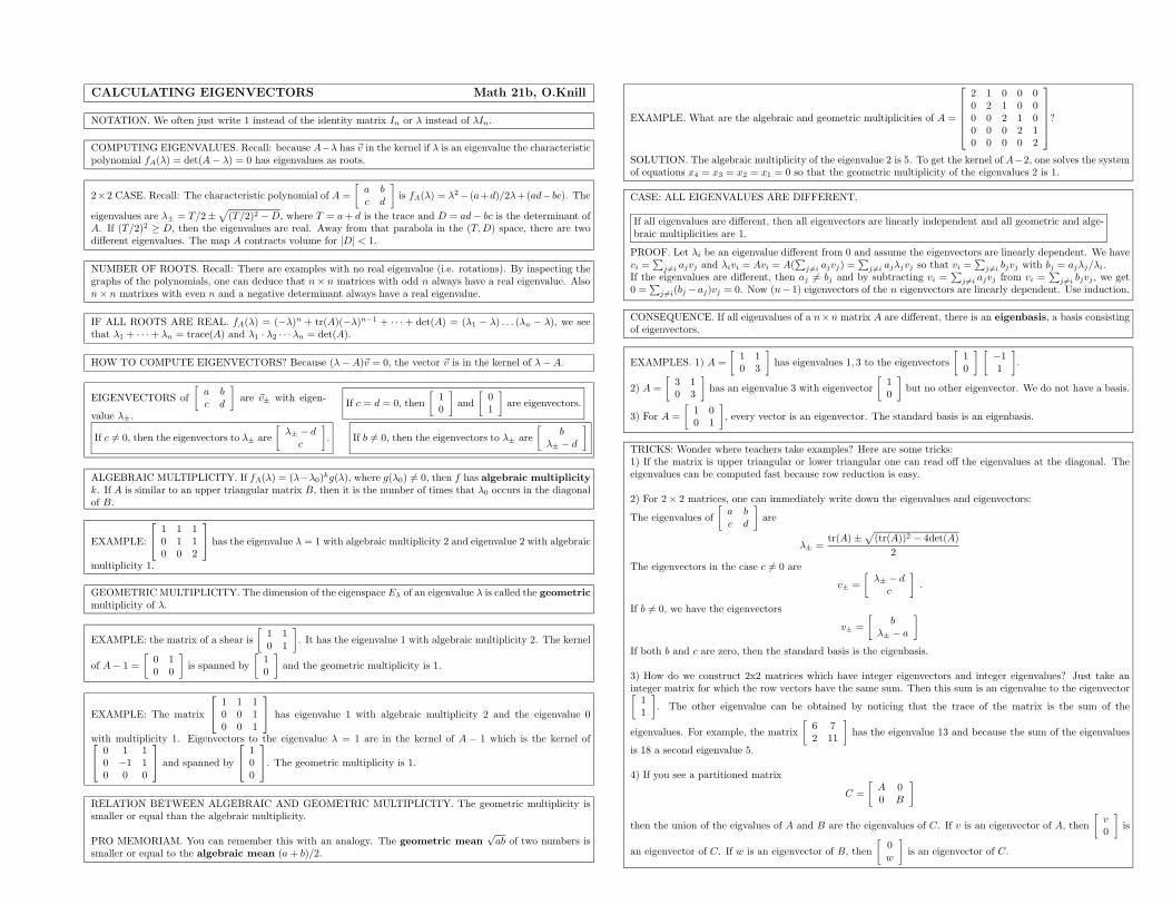
CALCULATING EIGENVECTORS Math 21b, O.Knill

NOTATION. We often just write 1 instead of the identity matrix In or λ instead of λIn.

COMPUTING EIGENVALUES. Recall: because A−λ has ~v in the kernel if λ is an eigenvalue the characteristicpolynomial fA(λ) = det(A− λ) = 0 has eigenvalues as roots.

2×2 CASE. Recall: The characteristic polynomial of A =

[

a bc d

]

is fA(λ) = λ2− (a+d)/2λ+(ad− bc). The

eigenvalues are λ± = T/2±√

(T/2)2 −D, where T = a+ d is the trace and D = ad− bc is the determinant ofA. If (T/2)2 ≥ D, then the eigenvalues are real. Away from that parabola in the (T,D) space, there are twodifferent eigenvalues. The map A contracts volume for |D| < 1.

NUMBER OF ROOTS. Recall: There are examples with no real eigenvalue (i.e. rotations). By inspecting thegraphs of the polynomials, one can deduce that n× n matrices with odd n always have a real eigenvalue. Alson× n matrixes with even n and a negative determinant always have a real eigenvalue.

IF ALL ROOTS ARE REAL. fA(λ) = (−λ)n + tr(A)(−λ)n−1 + · · · + det(A) = (λ1 − λ) . . . (λn − λ), we seethat λ1 + · · ·+ λn = trace(A) and λ1 · λ2 · · ·λn = det(A).

HOW TO COMPUTE EIGENVECTORS? Because (λ−A)~v = 0, the vector ~v is in the kernel of λ−A.

EIGENVECTORS of

[

a bc d

]

are ~v± with eigen-

value λ±.If c = d = 0, then

[

10

]

and

[

01

]

are eigenvectors.

If c 6= 0, then the eigenvectors to λ± are

[

λ± − dc

]

. If b 6= 0, then the eigenvectors to λ± are

[

bλ± − d

]

ALGEBRAIC MULTIPLICITY. If fA(λ) = (λ−λ0)kg(λ), where g(λ0) 6= 0, then f has algebraic multiplicity

k. If A is similar to an upper triangular matrix B, then it is the number of times that λ0 occurs in the diagonalof B.

EXAMPLE:

1 1 10 1 10 0 2

has the eigenvalue λ = 1 with algebraic multiplicity 2 and eigenvalue 2 with algebraic

multiplicity 1.

GEOMETRICMULTIPLICITY. The dimension of the eigenspace Eλ of an eigenvalue λ is called the geometric

multiplicity of λ.

EXAMPLE: the matrix of a shear is

[

1 10 1

]

. It has the eigenvalue 1 with algebraic multiplicity 2. The kernel

of A− 1 =

[

0 10 0

]

is spanned by

[

10

]

and the geometric multiplicity is 1.

EXAMPLE: The matrix

1 1 10 0 10 0 1

has eigenvalue 1 with algebraic multiplicity 2 and the eigenvalue 0

with multiplicity 1. Eigenvectors to the eigenvalue λ = 1 are in the kernel of A − 1 which is the kernel of

0 1 10 −1 10 0 0

and spanned by

100

. The geometric multiplicity is 1.

RELATION BETWEEN ALGEBRAIC AND GEOMETRIC MULTIPLICITY. The geometric multiplicity issmaller or equal than the algebraic multiplicity.

PRO MEMORIAM. You can remember this with an analogy. The geometric mean√ab of two numbers is

smaller or equal to the algebraic mean (a+ b)/2.

EXAMPLE. What are the algebraic and geometric multiplicities of A =

2 1 0 0 00 2 1 0 00 0 2 1 00 0 0 2 10 0 0 0 2

?

SOLUTION. The algebraic multiplicity of the eigenvalue 2 is 5. To get the kernel of A−2, one solves the systemof equations x4 = x3 = x2 = x1 = 0 so that the geometric multiplicity of the eigenvalues 2 is 1.

CASE: ALL EIGENVALUES ARE DIFFERENT.

If all eigenvalues are different, then all eigenvectors are linearly independent and all geometric and alge-braic multiplicities are 1.

PROOF. Let λi be an eigenvalue different from 0 and assume the eigenvectors are linearly dependent. We havevi =

∑

j 6=i ajvj and λivi = Avi = A(∑

j 6=i ajvj) =∑

j 6=i ajλjvj so that vi =∑

j 6=i bjvj with bj = ajλj/λi.If the eigenvalues are different, then aj 6= bj and by subtracting vi =

∑

j 6=i ajvj from vi =∑

j 6=i bjvj , we get0 =

∑

j 6=i(bj − aj)vj = 0. Now (n− 1) eigenvectors of the n eigenvectors are linearly dependent. Use induction.

CONSEQUENCE. If all eigenvalues of a n×n matrix A are different, there is an eigenbasis, a basis consistingof eigenvectors.

EXAMPLES. 1) A =

[

1 10 3

]

has eigenvalues 1, 3 to the eigenvectors

[

10

] [

−11

]

.

2) A =

[

3 10 3

]

has an eigenvalue 3 with eigenvector

[

10

]

but no other eigenvector. We do not have a basis.

3) For A =

[

1 00 1

]

, every vector is an eigenvector. The standard basis is an eigenbasis.

TRICKS: Wonder where teachers take examples? Here are some tricks:1) If the matrix is upper triangular or lower triangular one can read off the eigenvalues at the diagonal. Theeigenvalues can be computed fast because row reduction is easy.

2) For 2× 2 matrices, one can immediately write down the eigenvalues and eigenvectors:

The eigenvalues of

[

a bc d

]

are

λ± =tr(A)±

√

(tr(A))2 − 4det(A)

2

The eigenvectors in the case c 6= 0 are

v± =

[

λ± − dc

]

.

If b 6= 0, we have the eigenvectors

v± =

[

bλ± − a

]

If both b and c are zero, then the standard basis is the eigenbasis.

3) How do we construct 2x2 matrices which have integer eigenvectors and integer eigenvalues? Just take aninteger matrix for which the row vectors have the same sum. Then this sum is an eigenvalue to the eigenvector[

11

]

. The other eigenvalue can be obtained by noticing that the trace of the matrix is the sum of the

eigenvalues. For example, the matrix

[

6 72 11

]

has the eigenvalue 13 and because the sum of the eigenvalues

is 18 a second eigenvalue 5.

4) If you see a partitioned matrix

C =

[

A 00 B

]

then the union of the eigvalues of A and B are the eigenvalues of C. If v is an eigenvector of A, then

[

v0

]

is

an eigenvector of C. If w is an eigenvector of B, then

[

0w

]

is an eigenvector of C.

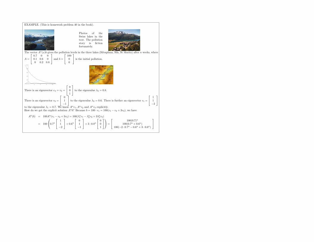
EXAMPLE. (This is homework problem 40 in the book).

Photos of theSwiss lakes in thetext. The pollutionstory is fictionfortunately.

The vector An(x)b gives the pollution levels in the three lakes (Silvaplana, Sils, St Moritz) after n weeks, where

A =

0.7 0 00.1 0.6 00 0.2 0.8

and b =

10000

is the initial pollution.

4 6 8 10

20

40

60

80

100

There is an eigenvector e3 = v3 =

001

to the eigenvalue λ3 = 0.8.

There is an eigenvector v2 =

01−1

to the eigenvalue λ2 = 0.6. There is further an eigenvector v1 =

11−2

to the eigenvalue λ1 = 0.7. We know Anv1, Anv2 and Anv3 explicitly.

How do we get the explicit solution Anb? Because b = 100 · e1 = 100(v1 − v2 + 3v3), we have

An(b) = 100An(v1 − v2 + 3v3) = 100(λn1v1 − λn

2v2 + 3λn

3v3)

= 100

0.7n

11−2

+ 0.6n

01−1

+ 3 · 0.8n

001

=

100(0.7)n

100(0.7n + 0.6n)100(−2 · 0.7n − 0.6n + 3 · 0.8n)

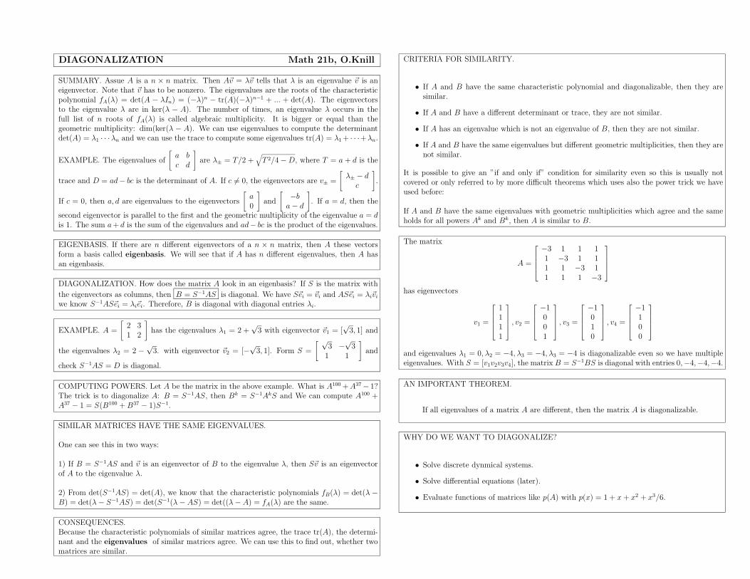
DIAGONALIZATION Math 21b, O.Knill

SUMMARY. Assue A is a n × n matrix. Then A~v = λ~v tells that λ is an eigenvalue ~v is aneigenvector. Note that ~v has to be nonzero. The eigenvalues are the roots of the characteristicpolynomial fA(λ) = det(A − λIn) = (−λ)n − tr(A)(−λ)n−1 + ... + det(A). The eigenvectorsto the eigenvalue λ are in ker(λ − A). The number of times, an eigenvalue λ occurs in thefull list of n roots of fA(λ) is called algebraic multiplicity. It is bigger or equal than thegeometric multiplicity: dim(ker(λ − A). We can use eigenvalues to compute the determinantdet(A) = λ1 · · ·λn and we can use the trace to compute some eigenvalues tr(A) = λ1+ · · ·+λn.

EXAMPLE. The eigenvalues of

[

a bc d

]

are λ± = T/2 +√

T 2/4−D, where T = a + d is the

trace and D = ad− bc is the determinant of A. If c 6= 0, the eigenvectors are v± =

[

λ± − dc

]

.

If c = 0, then a, d are eigenvalues to the eigenvectors

[

a0

]

and

[

−ba− d

]

. If a = d, then the

second eigenvector is parallel to the first and the geometric multiplicity of the eigenvalue a = dis 1. The sum a+ d is the sum of the eigenvalues and ad− bc is the product of the eigenvalues.

EIGENBASIS. If there are n different eigenvectors of a n × n matrix, then A these vectorsform a basis called eigenbasis. We will see that if A has n different eigenvalues, then A hasan eigenbasis.

DIAGONALIZATION. How does the matrix A look in an eigenbasis? If S is the matrix with

the eigenvectors as columns, then B = S−1AS is diagonal. We have S~ei = ~vi and AS~ei = λi~viwe know S−1AS~ei = λi~ei. Therefore, B is diagonal with diagonal entries λi.

EXAMPLE. A =

[

2 31 2

]

has the eigenvalues λ1 = 2 +√3 with eigenvector ~v1 = [

√3, 1] and

the eigenvalues λ2 = 2 −√3. with eigenvector ~v2 = [−

√3, 1]. Form S =

[ √3 −

√3

1 1

]

and

check S−1AS = D is diagonal.

COMPUTING POWERS. Let A be the matrix in the above example. What is A100 +A37− 1?The trick is to diagonalize A: B = S−1AS, then Bk = S−1AkS and We can compute A100 +A37 − 1 = S(B100 +B37 − 1)S−1.

SIMILAR MATRICES HAVE THE SAME EIGENVALUES.

One can see this in two ways:

1) If B = S−1AS and ~v is an eigenvector of B to the eigenvalue λ, then S~v is an eigenvectorof A to the eigenvalue λ.

2) From det(S−1AS) = det(A), we know that the characteristic polynomials fB(λ) = det(λ −B) = det(λ− S−1AS) = det(S−1(λ− AS) = det((λ−A) = fA(λ) are the same.

CONSEQUENCES.Because the characteristic polynomials of similar matrices agree, the trace tr(A), the determi-nant and the eigenvalues of similar matrices agree. We can use this to find out, whether twomatrices are similar.

CRITERIA FOR SIMILARITY.

• If A and B have the same characteristic polynomial and diagonalizable, then they aresimilar.

• If A and B have a different determinant or trace, they are not similar.

• If A has an eigenvalue which is not an eigenvalue of B, then they are not similar.

• If A and B have the same eigenvalues but different geometric multiplicities, then they arenot similar.

It is possible to give an ”if and only if” condition for similarity even so this is usually notcovered or only referred to by more difficult theorems which uses also the power trick we haveused before:

If A and B have the same eigenvalues with geometric multiplicities which agree and the sameholds for all powers Ak and Bk, then A is similar to B.

The matrix

A =

−3 1 1 11 −3 1 11 1 −3 11 1 1 −3

has eigenvectors

v1 =

1111

, v2 =

−1001

, v3 =

−1010

, v4 =

−1100

and eigenvalues λ1 = 0, λ2 = −4, λ3 = −4, λ3 = −4 is diagonalizable even so we have multipleeigenvalues. With S = [v1v2v3v4], the matrix B = S−1BS is diagonal with entries 0,−4,−4,−4.

AN IMPORTANT THEOREM.

If all eigenvalues of a matrix A are different, then the matrix A is diagonalizable.

WHY DO WE WANT TO DIAGONALIZE?

• Solve discrete dynmical systems.

• Solve differential equations (later).

• Evaluate functions of matrices like p(A) with p(x) = 1 + x+ x2 + x3/6.

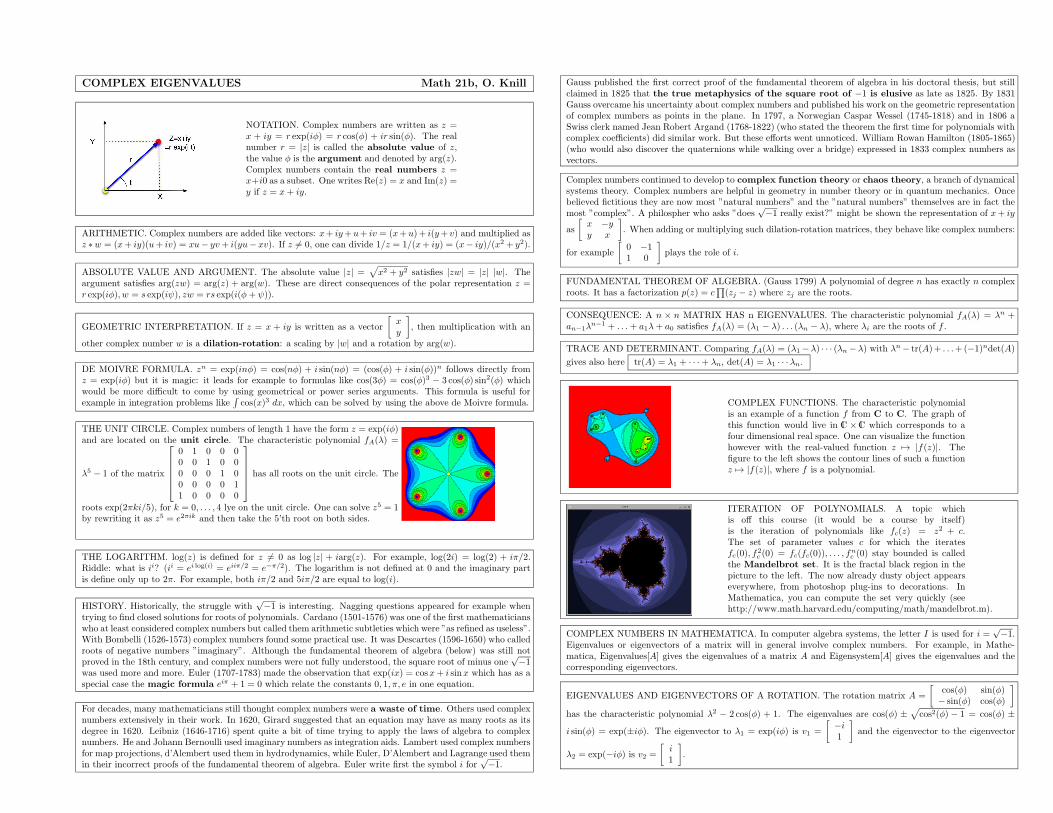
COMPLEX EIGENVALUES Math 21b, O. Knill

NOTATION. Complex numbers are written as z =x + iy = r exp(iφ) = r cos(φ) + ir sin(φ). The realnumber r = |z| is called the absolute value of z,the value φ is the argument and denoted by arg(z).Complex numbers contain the real numbers z =x+i0 as a subset. One writes Re(z) = x and Im(z) =y if z = x+ iy.

ARITHMETIC. Complex numbers are added like vectors: x+ iy+ u+ iv = (x+ u)+ i(y+ v) and multiplied asz ∗w = (x+ iy)(u+ iv) = xu− yv+ i(yu− xv). If z 6= 0, one can divide 1/z = 1/(x+ iy) = (x− iy)/(x2 + y2).

ABSOLUTE VALUE AND ARGUMENT. The absolute value |z| =√

x2 + y2 satisfies |zw| = |z| |w|. Theargument satisfies arg(zw) = arg(z) + arg(w). These are direct consequences of the polar representation z =r exp(iφ), w = s exp(iψ), zw = rs exp(i(φ+ ψ)).

GEOMETRIC INTERPRETATION. If z = x + iy is written as a vector

[

xy

]

, then multiplication with an

other complex number w is a dilation-rotation: a scaling by |w| and a rotation by arg(w).

DE MOIVRE FORMULA. zn = exp(inφ) = cos(nφ) + i sin(nφ) = (cos(φ) + i sin(φ))n follows directly fromz = exp(iφ) but it is magic: it leads for example to formulas like cos(3φ) = cos(φ)3 − 3 cos(φ) sin2(φ) whichwould be more difficult to come by using geometrical or power series arguments. This formula is useful forexample in integration problems like

∫

cos(x)3 dx, which can be solved by using the above de Moivre formula.

THE UNIT CIRCLE. Complex numbers of length 1 have the form z = exp(iφ)and are located on the unit circle. The characteristic polynomial fA(λ) =

λ5 − 1 of the matrix

0 1 0 0 00 0 1 0 00 0 0 1 00 0 0 0 11 0 0 0 0

has all roots on the unit circle. The

roots exp(2πki/5), for k = 0, . . . , 4 lye on the unit circle. One can solve z5 = 1by rewriting it as z5 = e2πik and then take the 5’th root on both sides.

THE LOGARITHM. log(z) is defined for z 6= 0 as log |z| + iarg(z). For example, log(2i) = log(2) + iπ/2.Riddle: what is ii? (ii = ei log(i) = eiiπ/2 = e−π/2). The logarithm is not defined at 0 and the imaginary partis define only up to 2π. For example, both iπ/2 and 5iπ/2 are equal to log(i).

HISTORY. Historically, the struggle with√−1 is interesting. Nagging questions appeared for example when

trying to find closed solutions for roots of polynomials. Cardano (1501-1576) was one of the first mathematicianswho at least considered complex numbers but called them arithmetic subtleties which were ”as refined as useless”.With Bombelli (1526-1573) complex numbers found some practical use. It was Descartes (1596-1650) who calledroots of negative numbers ”imaginary”. Although the fundamental theorem of algebra (below) was still notproved in the 18th century, and complex numbers were not fully understood, the square root of minus one

√−1

was used more and more. Euler (1707-1783) made the observation that exp(ix) = cosx+ i sinx which has as aspecial case the magic formula eiπ + 1 = 0 which relate the constants 0, 1, π, e in one equation.

For decades, many mathematicians still thought complex numbers were a waste of time. Others used complexnumbers extensively in their work. In 1620, Girard suggested that an equation may have as many roots as itsdegree in 1620. Leibniz (1646-1716) spent quite a bit of time trying to apply the laws of algebra to complexnumbers. He and Johann Bernoulli used imaginary numbers as integration aids. Lambert used complex numbersfor map projections, d’Alembert used them in hydrodynamics, while Euler, D’Alembert and Lagrange used themin their incorrect proofs of the fundamental theorem of algebra. Euler write first the symbol i for

√−1.

Gauss published the first correct proof of the fundamental theorem of algebra in his doctoral thesis, but stillclaimed in 1825 that the true metaphysics of the square root of −1 is elusive as late as 1825. By 1831Gauss overcame his uncertainty about complex numbers and published his work on the geometric representationof complex numbers as points in the plane. In 1797, a Norwegian Caspar Wessel (1745-1818) and in 1806 aSwiss clerk named Jean Robert Argand (1768-1822) (who stated the theorem the first time for polynomials withcomplex coefficients) did similar work. But these efforts went unnoticed. William Rowan Hamilton (1805-1865)(who would also discover the quaternions while walking over a bridge) expressed in 1833 complex numbers asvectors.

Complex numbers continued to develop to complex function theory or chaos theory, a branch of dynamicalsystems theory. Complex numbers are helpful in geometry in number theory or in quantum mechanics. Oncebelieved fictitious they are now most ”natural numbers” and the ”natural numbers” themselves are in fact themost ”complex”. A philospher who asks ”does

√−1 really exist?” might be shown the representation of x+ iy

as

[

x −yy x

]

. When adding or multiplying such dilation-rotation matrices, they behave like complex numbers:

for example

[

0 −11 0

]

plays the role of i.

FUNDAMENTAL THEOREM OF ALGEBRA. (Gauss 1799) A polynomial of degree n has exactly n complexroots. It has a factorization p(z) = c

∏

(zj − z) where zj are the roots.

CONSEQUENCE: A n × n MATRIX HAS n EIGENVALUES. The characteristic polynomial fA(λ) = λn +an−1λ

n−1 + . . .+ a1λ+ a0 satisfies fA(λ) = (λ1 − λ) . . . (λn − λ), where λi are the roots of f .

TRACE AND DETERMINANT. Comparing fA(λ) = (λ1 −λ) · · · (λn −λ) with λn − tr(A)+ . . .+(−1)ndet(A)

gives also here tr(A) = λ1 + · · ·+ λn, det(A) = λ1 · · ·λn.

COMPLEX FUNCTIONS. The characteristic polynomialis an example of a function f from C to C. The graph ofthis function would live in lC × lC which corresponds to afour dimensional real space. One can visualize the functionhowever with the real-valued function z 7→ |f(z)|. Thefigure to the left shows the contour lines of such a functionz 7→ |f(z)|, where f is a polynomial.

ITERATION OF POLYNOMIALS. A topic whichis off this course (it would be a course by itself)is the iteration of polynomials like fc(z) = z2 + c.The set of parameter values c for which the iteratesfc(0), f

2c (0) = fc(fc(0)), . . . , f

nc (0) stay bounded is called

the Mandelbrot set. It is the fractal black region in thepicture to the left. The now already dusty object appearseverywhere, from photoshop plug-ins to decorations. InMathematica, you can compute the set very quickly (seehttp://www.math.harvard.edu/computing/math/mandelbrot.m).

COMPLEX NUMBERS IN MATHEMATICA. In computer algebra systems, the letter I is used for i =√−1.

Eigenvalues or eigenvectors of a matrix will in general involve complex numbers. For example, in Mathe-matica, Eigenvalues[A] gives the eigenvalues of a matrix A and Eigensystem[A] gives the eigenvalues and thecorresponding eigenvectors.

EIGENVALUES AND EIGENVECTORS OF A ROTATION. The rotation matrix A =

[

cos(φ) sin(φ)− sin(φ) cos(φ)

]

has the characteristic polynomial λ2 − 2 cos(φ) + 1. The eigenvalues are cos(φ) ±√

cos2(φ) − 1 = cos(φ) ±i sin(φ) = exp(±iφ). The eigenvector to λ1 = exp(iφ) is v1 =

[

−i1

]

and the eigenvector to the eigenvector

λ2 = exp(−iφ) is v2 =

[

i1

]

.

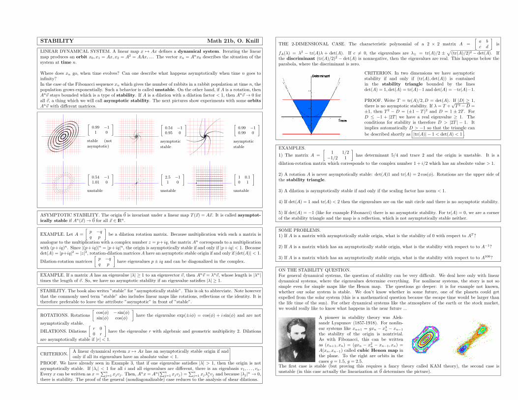
STABILITY Math 21b, O. Knill

LINEAR DYNAMICAL SYSTEM. A linear map x 7→ Ax defines a dynamical system. Iterating the linearmap produces an orbit x0, x1 = Ax, x2 = A2 = AAx, .... The vector xn = Anx0 describes the situation of thesystem at time n.

Where does xn go, when time evolves? Can one describe what happens asymptotically when time n goes toinfinity?In the case of the Fibonacci sequence xn which gives the number of rabbits in a rabbit population at time n, thepopulation grows exponentially. Such a behavior is called unstable. On the other hand, if A is a rotation, thenAn~v stays bounded which is a type of stability. If A is a dilation with a dilation factor < 1, then An~v → 0 forall ~v, a thing which we will call asymptotic stability. The next pictures show experiments with some orbits

An~v with different matrices.

[

0.99 −11 0

]

stable (not

asymptotic)

[

0.54 −10.95 0

]

asymptotic

stable

[

0.99 −10.99 0

]

asymptotic

stable

[

0.54 −11.01 0

]

unstable

[

2.5 −11 0

]

unstable

[

1 0.10 1

]

unstable

ASYMPTOTIC STABILITY. The origin ~0 is invariant under a linear map T (~x) = A~x. It is called asymptot-

ically stable if An(~x) → ~0 for all ~x ∈ IRn.

EXAMPLE. Let A =

[

p −qq p

]

be a dilation rotation matrix. Because multiplication wich such a matrix is

analogue to the multiplication with a complex number z = p+ iq, the matrix An corresponds to a multiplicationwith (p+ iq)n. Since |(p+ iq)|n = |p+ iq|n, the origin is asymptotically stable if and only if |p+ iq| < 1. Becausedet(A) = |p+iq|2 = |z|2, rotation-dilation matrices A have an asymptotic stable origin if and only if |det(A)| < 1.

Dilation-rotation matrices

[

p −qq p

]

have eigenvalues p± iq and can be diagonalized in the complex.

EXAMPLE. If a matrix A has an eigenvalue |λ| ≥ 1 to an eigenvector ~v, then An~v = λn~v, whose length is |λn|times the length of ~v. So, we have no asymptotic stability if an eigenvalue satisfies |λ| ≥ 1.

STABILITY. The book also writes ”stable” for ”asymptotically stable”. This is ok to abbreviate. Note howeverthat the commonly used term ”stable” also includes linear maps like rotations, reflections or the identity. It istherefore preferable to leave the attribute ”asymptotic” in front of ”stable”.

ROTATIONS. Rotations

[

cos(φ) − sin(φ)sin(φ) cos(φ)

]

have the eigenvalue exp(±iφ) = cos(φ) + i sin(φ) and are not

asymptotically stable.

DILATIONS. Dilations

[

r 00 r

]

have the eigenvalue r with algebraic and geometric multiplicity 2. Dilations

are asymptotically stable if |r| < 1.

CRITERION.A linear dynamical system x 7→ Ax has an asymptotically stable origin if andonly if all its eigenvalues have an absolute value < 1.

PROOF. We have already seen in Example 3, that if one eigenvalue satisfies |λ| > 1, then the origin is notasymptotically stable. If |λi| < 1 for all i and all eigenvalues are different, there is an eigenbasis v1, . . . , vn.Every x can be written as x =

∑n

j=1xjvj . Then, A

nx = An(∑n

j=1xjvj) =

∑n

j=1xjλ

nj vj and because |λj |n → 0,

there is stability. The proof of the general (nondiagonalizable) case reduces to the analysis of shear dilations.

THE 2-DIMENSIONAL CASE. The characteristic polynomial of a 2 × 2 matrix A =

[

a bc d

]

is

fA(λ) = λ2 − tr(A)λ + det(A). If c 6= 0, the eigenvalues are λ± = tr(A)/2 ±√

(tr(A)/2)2 − det(A). Ifthe discriminant (tr(A)/2)2 − det(A) is nonnegative, then the eigenvalues are real. This happens below theparabola, where the discriminant is zero.

CRITERION. In two dimensions we have asymptoticstability if and only if (tr(A), det(A)) is containedin the stability triangle bounded by the linesdet(A) = 1, det(A) = tr(A)−1 and det(A) = −tr(A)−1.

PROOF. Write T = tr(A)/2, D = det(A). If |D| ≥ 1,there is no asymptotic stability. If λ = T +

√T 2 −D =

±1, then T 2 − D = (±1 − T )2 and D = 1 ± 2T . ForD ≤ −1 + |2T | we have a real eigenvalue ≥ 1. Theconditions for stability is therefore D > |2T | − 1. Itimplies automatically D > −1 so that the triangle can

be described shortly as |tr(A)| − 1 < det(A) < 1 .

EXAMPLES.

1) The matrix A =

[

1 1/2−1/2 1

]

has determinant 5/4 and trace 2 and the origin is unstable. It is a

dilation-rotation matrix which corresponds to the complex number 1 + i/2 which has an absolute value > 1.

2) A rotation A is never asymptotically stable: det(A)1 and tr(A) = 2 cos(φ). Rotations are the upper side ofthe stability triangle.

3) A dilation is asymptotically stable if and only if the scaling factor has norm < 1.

4) If det(A) = 1 and tr(A) < 2 then the eigenvalues are on the unit circle and there is no asymptotic stability.

5) If det(A) = −1 (like for example Fibonacci) there is no asymptotic stability. For tr(A) = 0, we are a cornerof the stability triangle and the map is a reflection, which is not asymptotically stable neither.

SOME PROBLEMS.1) If A is a matrix with asymptotically stable origin, what is the stability of 0 with respect to AT ?

2) If A is a matrix which has an asymptotically stable origin, what is the stability with respect to to A−1?

3) If A is a matrix which has an asymptotically stable origin, what is the stability with respect to to A100?

ON THE STABILITY QUESTION.For general dynamical systems, the question of stability can be very difficult. We deal here only with lineardynamical systems, where the eigenvalues determine everything. For nonlinear systems, the story is not sosimple even for simple maps like the Henon map. The questions go deeper: it is for example not known,whether our solar system is stable. We don’t know whether in some future, one of the planets could getexpelled from the solar system (this is a mathematical question because the escape time would be larger thanthe life time of the sun). For other dynamical systems like the atmosphere of the earth or the stock market,we would really like to know what happens in the near future ...

A pioneer in stability theory was Alek-sandr Lyapunov (1857-1918). For nonlin-ear systems like xn+1 = gxn − x3

n − xn−1

the stability of the origin is nontrivial.As with Fibonacci, this can be writtenas (xn+1, xn) = (gxn − x2

n − xn−1, xn) =A(xn, xn−1) called cubic Henon map inthe plane. To the right are orbits in thecases g = 1.5, g = 2.5.

The first case is stable (but proving this requires a fancy theory called KAM theory), the second case isunstable (in this case actually the linearization at ~0 determines the picture).

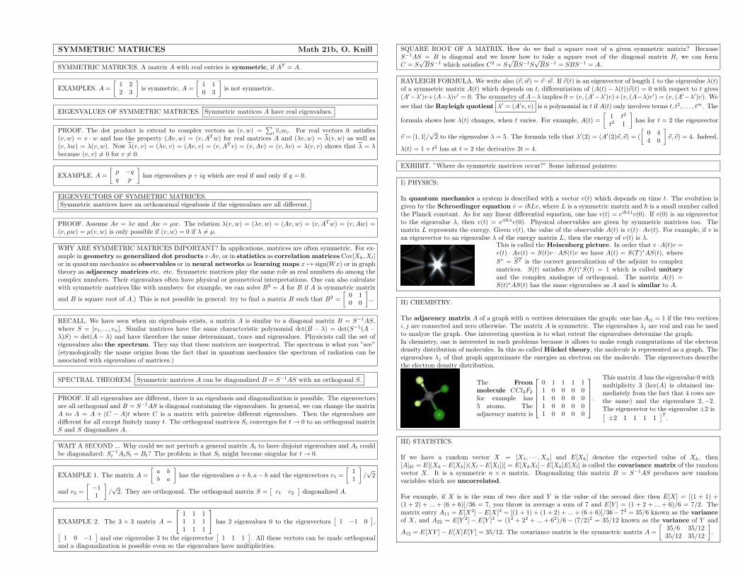
SYMMETRIC MATRICES Math 21b, O. Knill

SYMMETRIC MATRICES. A matrix A with real entries is symmetric, if AT = A.

EXAMPLES. A =

[

1 22 3

]

is symmetric, A =

[

1 10 3

]

is not symmetric.

EIGENVALUES OF SYMMETRIC MATRICES. Symmetric matrices A have real eigenvalues.

PROOF. The dot product is extend to complex vectors as (v, w) =∑

i viwi. For real vectors it satisfies(v, w) = v · w and has the property (Av,w) = (v,ATw) for real matrices A and (λv, w) = λ(v, w) as well as(v, λw) = λ(v, w). Now λ(v, v) = (λv, v) = (Av, v) = (v,AT v) = (v,Av) = (v, λv) = λ(v, v) shows that λ = λbecause (v, v) 6= 0 for v 6= 0.

EXAMPLE. A =

[

p −qq p

]

has eigenvalues p+ iq which are real if and only if q = 0.

EIGENVECTORS OF SYMMETRIC MATRICES.Symmetric matrices have an orthonormal eigenbasis if the eigenvalues are all different.

PROOF. Assume Av = λv and Aw = µw. The relation λ(v, w) = (λv, w) = (Av,w) = (v,ATw) = (v,Aw) =(v, µw) = µ(v, w) is only possible if (v, w) = 0 if λ 6= µ.

WHY ARE SYMMETRIC MATRICES IMPORTANT? In applications, matrices are often symmetric. For ex-ample in geometry as generalized dot products v·Av, or in statistics as correlation matrices Cov[Xk, Xl]or in quantum mechanics as observables or in neural networks as learning maps x 7→ sign(Wx) or in graphtheory as adjacency matrices etc. etc. Symmetric matrices play the same role as real numbers do among thecomplex numbers. Their eigenvalues often have physical or geometrical interpretations. One can also calculatewith symmetric matrices like with numbers: for example, we can solve B2 = A for B if A is symmetric matrix

and B is square root of A.) This is not possible in general: try to find a matrix B such that B2 =

[

0 10 0

]

...

RECALL. We have seen when an eigenbasis exists, a matrix A is similar to a diagonal matrix B = S−1AS,where S = [v1, ..., vn]. Similar matrices have the same characteristic polynomial det(B − λ) = det(S−1(A −λ)S) = det(A − λ) and have therefore the same determinant, trace and eigenvalues. Physicists call the set ofeigenvalues also the spectrum. They say that these matrices are isospectral. The spectrum is what you ”see”(etymologically the name origins from the fact that in quantum mechanics the spectrum of radiation can beassociated with eigenvalues of matrices.)

SPECTRAL THEOREM. Symmetric matrices A can be diagonalized B = S−1AS with an orthogonal S.

PROOF. If all eigenvalues are different, there is an eigenbasis and diagonalization is possible. The eigenvectorsare all orthogonal and B = S−1AS is diagonal containing the eigenvalues. In general, we can change the matrixA to A = A + (C − A)t where C is a matrix with pairwise different eigenvalues. Then the eigenvalues aredifferent for all except finitely many t. The orthogonal matrices St converges for t → 0 to an orthogonal matrixS and S diagonalizes A.

WAIT A SECOND ... Why could we not perturb a general matrix At to have disjoint eigenvalues and At couldbe diagonalized: S−1

t AtSt = Bt? The problem is that St might become singular for t → 0.

EXAMPLE 1. The matrix A =

[

a bb a

]

has the eigenvalues a+ b, a− b and the eigenvectors v1 =

[

11

]

/√2

and v2 =

[

−11

]

/√2. They are orthogonal. The orthogonal matrix S =

[

v1 v2]

diagonalized A.

EXAMPLE 2. The 3 × 3 matrix A =

1 1 11 1 11 1 1

has 2 eigenvalues 0 to the eigenvectors[

1 −1 0]

,

[

1 0 −1]

and one eigenvalue 3 to the eigenvector[

1 1 1]

. All these vectors can be made orthogonaland a diagonalization is possible even so the eigenvalues have multiplicities.

SQUARE ROOT OF A MATRIX. How do we find a square root of a given symmetric matrix? BecauseS−1AS = B is diagonal and we know how to take a square root of the diagonal matrix B, we can formC = S

√BS−1 which satisfies C2 = S

√BS−1S

√BS−1 = SBS−1 = A.

RAYLEIGH FORMULA. We write also (~v, ~w) = ~v · ~w. If ~v(t) is an eigenvector of length 1 to the eigenvalue λ(t)of a symmetric matrix A(t) which depends on t, differentiation of (A(t) − λ(t))~v(t) = 0 with respect to t gives(A′−λ′)v+(A−λ)v′ = 0. The symmetry of A−λ implies 0 = (v, (A′−λ′)v)+(v, (A−λ)v′) = (v, (A′−λ′)v). We

see that the Rayleigh quotient λ′ = (A′v, v) is a polynomial in t if A(t) only involves terms t, t2, . . . , tm. The

formula shows how λ(t) changes, when t varies. For example, A(t) =

[

1 t2

t2 1

]

has for t = 2 the eigenvector

~v = [1, 1]/√2 to the eigenvalue λ = 5. The formula tells that λ′(2) = (A′(2)~v,~v) = (

[

0 44 0

]

~v,~v) = 4. Indeed,

λ(t) = 1 + t2 has at t = 2 the derivative 2t = 4.

EXHIBIT. ”Where do symmetric matrices occur?” Some informal pointers:

I) PHYSICS:

In quantum mechanics a system is described with a vector v(t) which depends on time t. The evolution isgiven by the Schroedinger equation v = ihLv, where L is a symmetric matrix and h is a small number calledthe Planck constant. As for any linear differential equation, one has v(t) = eihLtv(0). If v(0) is an eigenvectorto the eigenvalue λ, then v(t) = eithλv(0). Physical observables are given by symmetric matrices too. Thematrix L represents the energy. Given v(t), the value of the observable A(t) is v(t) ·Av(t). For example, if v isan eigenvector to an eigenvalue λ of the energy matrix L, then the energy of v(t) is λ.

This is called the Heisenberg picture. In order that v ·A(t)v =v(t) · Av(t) = S(t)v · AS(t)v we have A(t) = S(T )∗AS(t), where

S∗ = ST is the correct generalization of the adjoint to complexmatrices. S(t) satisfies S(t)∗S(t) = 1 which is called unitary

and the complex analogue of orthogonal. The matrix A(t) =S(t)∗AS(t) has the same eigenvalues as A and is similar to A.

II) CHEMISTRY.

The adjacency matrix A of a graph with n vertices determines the graph: one has Aij = 1 if the two verticesi, j are connected and zero otherwise. The matrix A is symmetric. The eigenvalues λj are real and can be usedto analyze the graph. One interesting question is to what extent the eigenvalues determine the graph.In chemistry, one is interested in such problems because it allows to make rough computations of the electrondensity distribution of molecules. In this so called Huckel theory, the molecule is represented as a graph. Theeigenvalues λj of that graph approximate the energies an electron on the molecule. The eigenvectors describethe electron density distribution.

The Freon

molecule CCl2F2

for example has5 atoms. Theadjacency matrix is

0 1 1 1 11 0 0 0 01 0 0 0 01 0 0 0 01 0 0 0 0

.

This matrix A has the eigenvalue 0 withmultiplicity 3 (ker(A) is obtained im-mediately from the fact that 4 rows arethe same) and the eigenvalues 2,−2.The eigenvector to the eigenvalue ±2 is[

±2 1 1 1 1]T

.

III) STATISTICS.

If we have a random vector X = [X1, · · · , Xn] and E[Xk] denotes the expected value of Xk, then[A]kl = E[(Xk −E[Xk])(Xl−E[Xl])] = E[XkXl]−E[Xk]E[Xl] is called the covariance matrix of the randomvector X . It is a symmetric n × n matrix. Diagonalizing this matrix B = S−1AS produces new randomvariables which are uncorrelated.

For example, if X is is the sum of two dice and Y is the value of the second dice then E[X ] = [(1 + 1) +(1 + 2) + ... + (6 + 6)]/36 = 7, you throw in average a sum of 7 and E[Y ] = (1 + 2 + ... + 6)/6 = 7/2. Thematrix entry A11 = E[X2]− E[X ]2 = [(1 + 1) + (1 + 2) + ...+ (6 + 6)]/36− 72 = 35/6 known as the variance

of X , and A22 = E[Y 2] − E[Y ]2 = (12 + 22 + ... + 62)/6 − (7/2)2 = 35/12 known as the variance of Y and

A12 = E[XY ]− E[X ]E[Y ] = 35/12. The covariance matrix is the symmetric matrix A =

[

35/6 35/1235/12 35/12

]

.

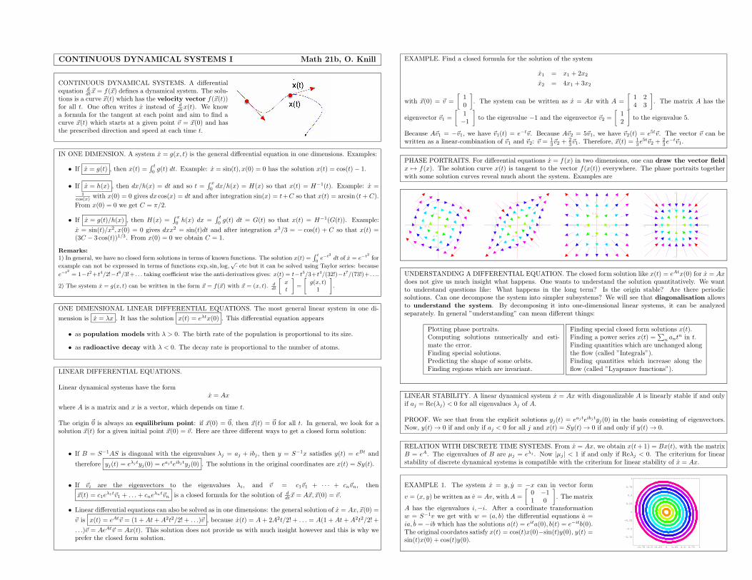
CONTINUOUS DYNAMICAL SYSTEMS I Math 21b, O. Knill

CONTINUOUS DYNAMICAL SYSTEMS. A differentialequation d

dt~x = f(~x) defines a dynamical system. The solu-tions is a curve ~x(t) which has the velocity vector f(~x(t))for all t. One often writes x instead of d

dtx(t). We knowa formula for the tangent at each point and aim to find acurve ~x(t) which starts at a given point ~v = ~x(0) and hasthe prescribed direction and speed at each time t.

IN ONE DIMENSION. A system x = g(x, t) is the general differential equation in one dimensions. Examples:

• If x = g(t) , then x(t) =∫ t

0 g(t) dt. Example: x = sin(t), x(0) = 0 has the solution x(t) = cos(t)− 1.

• If x = h(x) , then dx/h(x) = dt and so t =∫ x

0 dx/h(x) = H(x) so that x(t) = H−1(t). Example: x =1

cos(x) with x(0) = 0 gives dx cos(x) = dt and after integration sin(x) = t+C so that x(t) = arcsin (t+ C).

From x(0) = 0 we get C = π/2.

• If x = g(t)/h(x) , then H(x) =∫ x

0 h(x) dx =∫ t

0 g(t) dt = G(t) so that x(t) = H−1(G(t)). Example:

x = sin(t)/x2, x(0) = 0 gives dxx2 = sin(t)dt and after integration x3/3 = − cos(t) + C so that x(t) =(3C − 3 cos(t))1/3. From x(0) = 0 we obtain C = 1.

Remarks:

1) In general, we have no closed form solutions in terms of known functions. The solution x(t) =∫

t

0e−t

2

dt of x = e−t2

for

example can not be expressed in terms of functions exp, sin, log,√· etc but it can be solved using Taylor series: because

e−t2

= 1−t2+t4/2!−t6/3!+ . . . taking coefficient wise the anti-derivatives gives: x(t) = t−t3/3+t4/(32!)−t7/(73!)+ . . ..

2) The system x = g(x, t) can be written in the form ~x = f(~x) with ~x = (x, t). d

dt

[

xt

]

=

[

g(x, t)1

]

.

ONE DIMENSIONAL LINEAR DIFFERENTIAL EQUATIONS. The most general linear system in one di-

mension is x = λx . It has the solution x(t) = eλtx(0) . This differential equation appears

• as population models with λ > 0. The birth rate of the population is proportional to its size.

• as radioactive decay with λ < 0. The decay rate is proportional to the number of atoms.

LINEAR DIFFERENTIAL EQUATIONS.

Linear dynamical systems have the formx = Ax

where A is a matrix and x is a vector, which depends on time t.

The origin ~0 is always an equilibrium point: if ~x(0) = ~0, then ~x(t) = ~0 for all t. In general, we look for asolution ~x(t) for a given initial point ~x(0) = ~v. Here are three different ways to get a closed form solution:

• If B = S−1AS is diagonal with the eigenvalues λj = aj + ibj, then y = S−1x satisfies y(t) = eBt and

therefore yj(t) = eλjtyj(0) = eajteibjtyj(0) . The solutions in the original coordinates are x(t) = Sy(t).

• If ~vi are the eigenvectors to the eigenvalues λi, and ~v = c1~v1 + · · · + cn~vn, then

~x(t) = c1eλ1t~v1 + . . .+ cne

λnt~vn is a closed formula for the solution of ddt~x = A~x, ~x(0) = ~v.

• Linear differential equations can also be solved as in one dimensions: the general solution of x = Ax, ~x(0) =

~v is x(t) = eAt~v = (1 +At+A2t2/2! + . . .)~v , because x(t) = A+ 2A2t/2! + . . . = A(1 +At+A2t2/2! +

. . .)~v = AeAt~v = Ax(t). This solution does not provide us with much insight however and this is why weprefer the closed form solution.

EXAMPLE. Find a closed formula for the solution of the system

x1 = x1 + 2x2

x2 = 4x1 + 3x2

with ~x(0) = ~v =

[

10

]

. The system can be written as x = Ax with A =

[

1 24 3

]

. The matrix A has the

eigenvector ~v1 =

[

1−1

]

to the eigenvalue −1 and the eigenvector ~v2 =

[

12

]

to the eigenvalue 5.

Because A~v1 = −~v1, we have ~v1(t) = e−t~v. Because A~v2 = 5~v1, we have ~v2(t) = e5t~v. The vector ~v can bewritten as a linear-combination of ~v1 and ~v2: ~v = 1

3~v2 +23~v1. Therefore, ~x(t) =

13e

5t~v2 +23e

−t~v1.

PHASE PORTRAITS. For differential equations x = f(x) in two dimensions, one can draw the vector field

x 7→ f(x). The solution curve x(t) is tangent to the vector f(x(t)) everywhere. The phase portraits togetherwith some solution curves reveal much about the system. Examples are

-1 -0.5 0.5 1

-1

-0.5

0.5

1

-1 -0.5 0.5 1

-1

-0.5

0.5

1

-1 -0.5 0.5 1

-1

-0.5

0.5

1

-1 -0.5 0.5 1

-1

-0.5

0.5

1

UNDERSTANDING A DIFFERENTIAL EQUATION. The closed form solution like x(t) = eAtx(0) for x = Axdoes not give us much insight what happens. One wants to understand the solution quantitatively. We wantto understand questions like: What happens in the long term? Is the origin stable? Are there periodicsolutions. Can one decompose the system into simpler subsystems? We will see that diagonalisation allowsto understand the system. By decomposing it into one-dimensional linear systems, it can be analyzedseparately. In general ”understanding” can mean different things:

Plotting phase portraits.Computing solutions numerically and esti-mate the error.Finding special solutions.Predicting the shape of some orbits.Finding regions which are invariant.

Finding special closed form solutions x(t).Finding a power series x(t) =

∑

n antn in t.

Finding quantities which are unchanged alongthe flow (called ”Integrals”).Finding quantities which increase along theflow (called ”Lyapunov functions”).

LINEAR STABILITY. A linear dynamical system x = Ax with diagonalizable A is linearly stable if and onlyif aj = Re(λj) < 0 for all eigenvalues λj of A.

PROOF. We see that from the explicit solutions yj(t) = eajteibj tyj(0) in the basis consisting of eigenvectors.Now, y(t) → 0 if and only if aj < 0 for all j and x(t) = Sy(t) → 0 if and only if y(t) → 0.

RELATION WITH DISCRETE TIME SYSTEMS. From x = Ax, we obtain x(t+ 1) = Bx(t), with the matrixB = eA. The eigenvalues of B are µj = eλj . Now |µj | < 1 if and only if Reλj < 0. The criterium for linearstability of discrete dynamical systems is compatible with the criterium for linear stability of x = Ax.

EXAMPLE 1. The system x = y, y = −x can in vector form

v = (x, y) be written as v = Av, with A =

[

0 −11 0

]

. The matrix

A has the eigenvalues i,−i. After a coordinate transformationw = S−1v we get with w = (a, b) the differential equations a =ia, b = −ib which has the solutions a(t) = eita(0), b(t) = e−itb(0).The original coordates satisfy x(t) = cos(t)x(0)−sin(t)y(0), y(t) =sin(t)x(0) + cos(t)y(0).

-0.75 -0.5 -0.25 0 0.25 0.5 0.75 1

-0.75

-0.5

-0.25

0

0.25

0.5

0.75

1

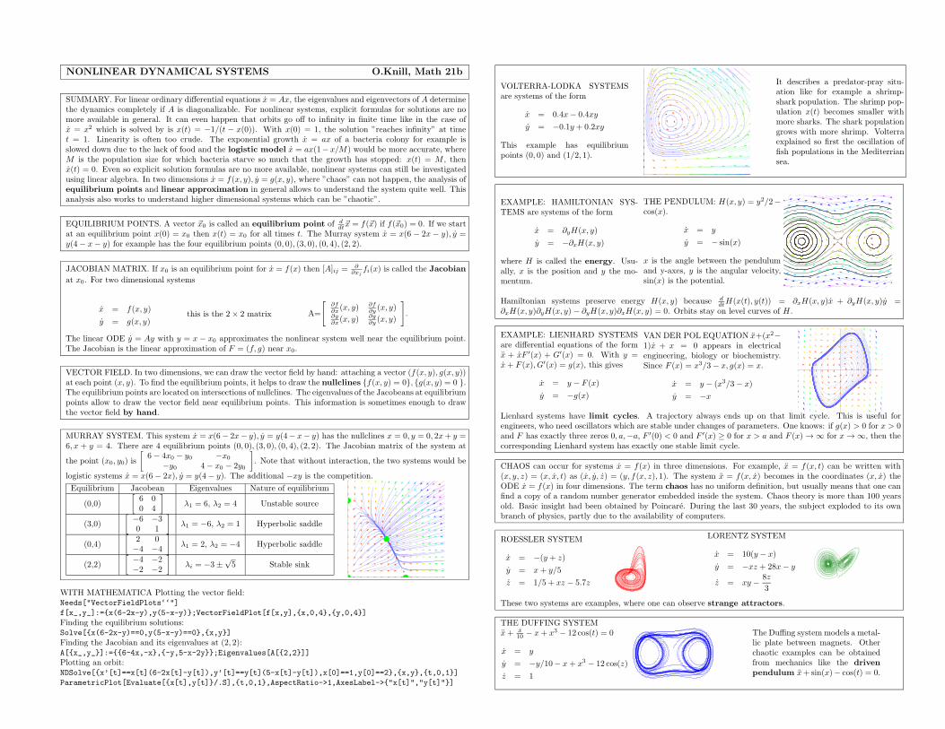
NONLINEAR DYNAMICAL SYSTEMS O.Knill, Math 21b

SUMMARY. For linear ordinary differential equations x = Ax, the eigenvalues and eigenvectors of A determinethe dynamics completely if A is diagonalizable. For nonlinear systems, explicit formulas for solutions are nomore available in general. It can even happen that orbits go off to infinity in finite time like in the case ofx = x2 which is solved by is x(t) = −1/(t − x(0)). With x(0) = 1, the solution ”reaches infinity” at timet = 1. Linearity is often too crude. The exponential growth x = ax of a bacteria colony for example isslowed down due to the lack of food and the logistic model x = ax(1− x/M) would be more accurate, whereM is the population size for which bacteria starve so much that the growth has stopped: x(t) = M , thenx(t) = 0. Even so explicit solution formulas are no more available, nonlinear systems can still be investigatedusing linear algebra. In two dimensions x = f(x, y), y = g(x, y), where ”chaos” can not happen, the analysis ofequilibrium points and linear approximation in general allows to understand the system quite well. Thisanalysis also works to understand higher dimensional systems which can be ”chaotic”.

EQUILIBRIUM POINTS. A vector ~x0 is called an equilibrium point of ddt~x = f(~x) if f(~x0) = 0. If we start

at an equilibrium point x(0) = x0 then x(t) = x0 for all times t. The Murray system x = x(6 − 2x − y), y =y(4− x− y) for example has the four equilibrium points (0, 0), (3, 0), (0, 4), (2, 2).

JACOBIAN MATRIX. If x0 is an equilibrium point for x = f(x) then [A]ij =∂

∂xjfi(x) is called the Jacobian

at x0. For two dimensional systems

x = f(x, y)

y = g(x, y)this is the 2× 2 matrix A=

[

∂f∂x

(x, y) ∂f∂y

(x, y)∂g∂x

(x, y) ∂g∂y

(x, y)

]

.

The linear ODE y = Ay with y = x − x0 approximates the nonlinear system well near the equilibrium point.The Jacobian is the linear approximation of F = (f, g) near x0.

VECTOR FIELD. In two dimensions, we can draw the vector field by hand: attaching a vector (f(x, y), g(x, y))at each point (x, y). To find the equilibrium points, it helps to draw the nullclines {f(x, y) = 0}, {g(x, y) = 0 }.The equilibrium points are located on intersections of nullclines. The eigenvalues of the Jacobeans at equilibriumpoints allow to draw the vector field near equilibrium points. This information is sometimes enough to drawthe vector field by hand.

MURRAY SYSTEM. This system x = x(6− 2x− y), y = y(4− x− y) has the nullclines x = 0, y = 0, 2x+ y =6, x + y = 4. There are 4 equilibrium points (0, 0), (3, 0), (0, 4), (2, 2). The Jacobian matrix of the system at

the point (x0, y0) is

[

6− 4x0 − y0 −x0

−y0 4− x0 − 2y0

]

. Note that without interaction, the two systems would be

logistic systems x = x(6 − 2x), y = y(4− y). The additional −xy is the competition.

Equilibrium Jacobean Eigenvalues Nature of equilibrium

(0,0)

[

6 00 4

]

λ1 = 6, λ2 = 4 Unstable source

(3,0)

[

−6 −30 1

]

λ1 = −6, λ2 = 1 Hyperbolic saddle

(0,4)

[

2 0−4 −4

]

λ1 = 2, λ2 = −4 Hyperbolic saddle

(2,2)

[

−4 −2−2 −2

]

λi = −3±√5 Stable sink

WITH MATHEMATICA Plotting the vector field:Needs["VectorFieldPlots‘‘"]

f[x_,y_]:={x(6-2x-y),y(5-x-y)};VectorFieldPlot[f[x,y],{x,0,4},{y,0,4}]

Finding the equilibrium solutions:Solve[{x(6-2x-y)==0,y(5-x-y)==0},{x,y}]

Finding the Jacobian and its eigenvalues at (2, 2):A[{x_,y_}]:={{6-4x,-x},{-y,5-x-2y}};Eigenvalues[A[{2,2}]]

Plotting an orbit:NDSolve[{x’[t]==x[t](6-2x[t]-y[t]),y’[t]==y[t](5-x[t]-y[t]),x[0]==1,y[0]==2},{x,y},{t,0,1}]

ParametricPlot[Evaluate[{x[t],y[t]}/.S],{t,0,1},AspectRatio->1,AxesLabel->{"x[t]","y[t]"}]

VOLTERRA-LODKA SYSTEMSare systems of the form

x = 0.4x− 0.4xy

y = −0.1y + 0.2xy

This example has equilibriumpoints (0, 0) and (1/2, 1).

It describes a predator-pray situ-ation like for example a shrimp-shark population. The shrimp pop-ulation x(t) becomes smaller withmore sharks. The shark populationgrows with more shrimp. Volterraexplained so first the oscillation offish populations in the Mediterriansea.

EXAMPLE: HAMILTONIAN SYS-TEMS are systems of the form

x = ∂yH(x, y)

y = −∂xH(x, y)

where H is called the energy. Usu-ally, x is the position and y the mo-mentum.

THE PENDULUM: H(x, y) = y2/2−cos(x).

x = y

y = − sin(x)

x is the angle between the pendulumand y-axes, y is the angular velocity,sin(x) is the potential.

Hamiltonian systems preserve energy H(x, y) because ddtH(x(t), y(t)) = ∂xH(x, y)x + ∂yH(x, y)y =

∂xH(x, y)∂yH(x, y)− ∂yH(x, y)∂xH(x, y) = 0. Orbits stay on level curves of H .

EXAMPLE: LIENHARD SYSTEMSare differential equations of the formx + xF ′(x) + G′(x) = 0. With y =x+ F (x), G′(x) = g(x), this gives

x = y − F (x)

y = −g(x)

VAN DER POL EQUATION x+(x2−1)x + x = 0 appears in electricalengineering, biology or biochemistry.Since F (x) = x3/3− x, g(x) = x.

x = y − (x3/3− x)

y = −x

Lienhard systems have limit cycles. A trajectory always ends up on that limit cycle. This is useful forengineers, who need oscillators which are stable under changes of parameters. One knows: if g(x) > 0 for x > 0and F has exactly three zeros 0, a,−a, F ′(0) < 0 and F ′(x) ≥ 0 for x > a and F (x) → ∞ for x → ∞, then thecorresponding Lienhard system has exactly one stable limit cycle.

CHAOS can occur for systems x = f(x) in three dimensions. For example, x = f(x, t) can be written with(x, y, z) = (x, x, t) as (x, y, z) = (y, f(x, z), 1). The system x = f(x, x) becomes in the coordinates (x, x) theODE x = f(x) in four dimensions. The term chaos has no uniform definition, but usually means that one canfind a copy of a random number generator embedded inside the system. Chaos theory is more than 100 yearsold. Basic insight had been obtained by Poincare. During the last 30 years, the subject exploded to its ownbranch of physics, partly due to the availability of computers.

ROESSLER SYSTEM

x = −(y + z)

y = x+ y/5

z = 1/5 + xz − 5.7z

LORENTZ SYSTEM

x = 10(y − x)

y = −xz + 28x− y

z = xy − 8z

3

These two systems are examples, where one can observe strange attractors.

THE DUFFING SYSTEMx+ x

10− x+ x3 − 12 cos(t) = 0

x = y

y = −y/10− x+ x3 − 12 cos(z)

z = 1

The Duffing system models a metal-lic plate between magnets. Otherchaotic examples can be obtainedfrom mechanics like the driven

pendulum x+ sin(x)− cos(t) = 0.

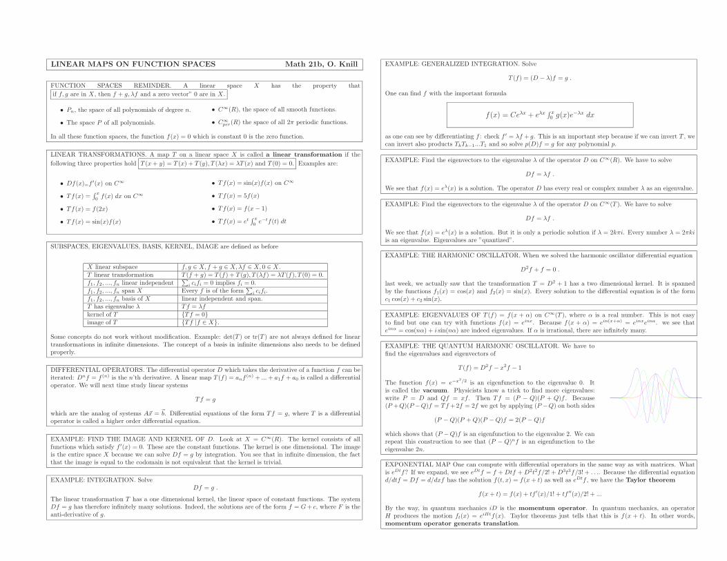
LINEAR MAPS ON FUNCTION SPACES Math 21b, O. Knill

FUNCTION SPACES REMINDER. A linear space X has the property that

if f, g are in X , then f + g, λf and a zero vector” 0 are in X .

• Pn, the space of all polynomials of degree n.

• The space P of all polynomials.

• C∞(R), the space of all smooth functions.

• C∞

per(R) the space of all 2π periodic functions.

In all these function spaces, the function f(x) = 0 which is constant 0 is the zero function.

LINEAR TRANSFORMATIONS. A map T on a linear space X is called a linear transformation if the

following three properties hold T (x+ y) = T (x) + T (y), T (λx) = λT (x) and T (0) = 0. Examples are:

• Df(x)=f′(x) on C∞

• Tf(x) =∫ x

0 f(x) dx on C∞

• Tf(x) = f(2x)

• Tf(x) = sin(x)f(x)

• Tf(x) = sin(x)f(x) on C∞

• Tf(x) = 5f(x)

• Tf(x) = f(x− 1)

• Tf(x) = et∫ x

0e−tf(t) dt

SUBSPACES, EIGENVALUES, BASIS, KERNEL, IMAGE are defined as before

X linear subspace f, g ∈ X, f + g ∈ X,λf ∈ X, 0 ∈ X .T linear transformation T (f + g) = T (f) + T (g), T (λf) = λT (f), T (0) = 0.f1, f2, ..., fn linear independent

∑i cifi = 0 implies fi = 0.

f1, f2, ..., fn span X Every f is of the form∑

i cifi.f1, f2, ..., fn basis of X linear independent and span.T has eigenvalue λ Tf = λfkernel of T {Tf = 0}image of T {Tf |f ∈ X}.

Some concepts do not work without modification. Example: det(T ) or tr(T ) are not always defined for lineartransformations in infinite dimensions. The concept of a basis in infinite dimensions also needs to be definedproperly.

DIFFERENTIAL OPERATORS. The differential operator D which takes the derivative of a function f can beiterated: Dnf = f (n) is the n’th derivative. A linear map T (f) = anf

(n) + ...+ a1f + a0 is called a differentialoperator. We will next time study linear systems

Tf = g

which are the analog of systems A~x = ~b. Differential equations of the form Tf = g, where T is a differentialoperator is called a higher order differential equation.

EXAMPLE: FIND THE IMAGE AND KERNEL OF D. Look at X = C∞(R). The kernel consists of allfunctions which satisfy f ′(x) = 0. These are the constant functions. The kernel is one dimensional. The imageis the entire space X because we can solve Df = g by integration. You see that in infinite dimension, the factthat the image is equal to the codomain is not equivalent that the kernel is trivial.

EXAMPLE: INTEGRATION. SolveDf = g .

The linear transformation T has a one dimensional kernel, the linear space of constant functions. The systemDf = g has therefore infinitely many solutions. Indeed, the solutions are of the form f = G+ c, where F is theanti-derivative of g.

EXAMPLE: GENERALIZED INTEGRATION. Solve

T (f) = (D − λ)f = g .

One can find f with the important formula

f(x) = Ceλx + eλx∫x

0g(x)e−λx dx

as one can see by differentiating f : check f ′ = λf + g. This is an important step because if we can invert T , wecan invert also products TkTk−1...T1 and so solve p(D)f = g for any polynomial p.

EXAMPLE: Find the eigenvectors to the eigenvalue λ of the operator D on C∞(R). We have to solve

Df = λf .

We see that f(x) = eλ(x) is a solution. The operator D has every real or complex number λ as an eigenvalue.

EXAMPLE: Find the eigenvectors to the eigenvalue λ of the operator D on C∞(T ). We have to solve

Df = λf .

We see that f(x) = eλ(x) is a solution. But it is only a periodic solution if λ = 2kπi. Every number λ = 2πkiis an eigenvalue. Eigenvalues are ”quantized”.

EXAMPLE: THE HARMONIC OSCILLATOR. When we solved the harmonic oscillator differential equation

D2f + f = 0 .

last week, we actually saw that the transformation T = D2 + 1 has a two dimensional kernel. It is spannedby the functions f1(x) = cos(x) and f2(x) = sin(x). Every solution to the differential equation is of the formc1 cos(x) + c2 sin(x).

EXAMPLE: EIGENVALUES OF T (f) = f(x + α) on C∞(T ), where α is a real number. This is not easyto find but one can try with functions f(x) = einx. Because f(x + α) = ein(x+α) = einxeinα. we see thateinα = cos(nα) + i sin(nα) are indeed eigenvalues. If α is irrational, there are infinitely many.

EXAMPLE: THE QUANTUM HARMONIC OSCILLATOR. We have tofind the eigenvalues and eigenvectors of

T (f) = D2f − x2f − 1

The function f(x) = e−x2/2 is an eigenfunction to the eigenvalue 0. Itis called the vacuum. Physicists know a trick to find more eigenvalues:write P = D and Qf = xf . Then Tf = (P − Q)(P + Q)f . Because(P +Q)(P −Q)f = Tf +2f = 2f we get by applying (P −Q) on both sides

(P −Q)(P +Q)(P −Q)f = 2(P −Q)f

which shows that (P −Q)f is an eigenfunction to the eigenvalue 2. We canrepeat this construction to see that (P − Q)nf is an eigenfunction to theeigenvalue 2n.

EXPONENTIAL MAP One can compute with differential operators in the same way as with matrices. Whatis eDtf? If we expand, we see eDtf = f +Dtf +D2t2f/2! +D3t3f/3! + . . .. Because the differential equationd/dtf = Df = d/dxf has the solution f(t, x) = f(x+ t) as well as eDtf , we have the Taylor theorem

f(x+ t) = f(x) + tf ′(x)/1! + tf ′′(x)/2! + ...

By the way, in quantum mechanics iD is the momentum operator. In quantum mechanics, an operatorH produces the motion ft(x) = eiHtf(x). Taylor theorems just tells that this is f(x + t). In other words,momentum operator generats translation.

DIFFERENTIAL OPERATORS Math 21b, 2010

The handout contains the homework for Fri-day November 19, 2010. The topic are lineartransformation on the linear space X = C∞

of smooth functions. Remember that a func-tion is called smooth, if we can differentiateit arbitrarily many times.

Examples: f(x) = sin(x) + x2 is anelement in C∞. The function f(x) =|x|5/2 is not in X since its third deriva-tive is no more defined at 0. The con-stant function f(x) = 2 is in X .

X is a linear space because it contains the zero function and if f, g are in X then f + g, λf

are in X . All the concepts introduced for vectors can be used for functions. The terminologycan shift. An eigenvector is also called eigenfunction.

A map T : C∞ → C∞ is called a linear operator onX if the following three conditions are are satisfied:

(i) T (f + g) = T (f) + T (g)(ii) T (λf) = λT (f)(iii) T (0) = 0.

An important example of a linear operator is the differ-entiation operator D. If p is a polynomial, we can formp(D). For example, for p(x) = x2 + 3x − 2 we obtainp(D) = D2 + 3D + 2 and get p(D)f = f ′′ + 3f ′ + 2f .

D(f) = f ′

p(D) differential opera-tor

Problem 1) Which of the following maps are linear operators?

a) T (f)(x) = x2f(x− 4)b) T (f)(x) = f ′(x)2

c) T = D2 +D + 1 meaning T (f)(x) = f ′′(x) + f ′(x) + f(x).d) T (f)(x) = ex

∫ x0e−tf(t) dt.

Problem 2) a) What is the kernel and image of the linear operators T = D + 3 and

D − 2? Use this to find the kernel of p(D) for p(x) = x2 + x− 6?b) Verify whether the function f(x) = xe−x2/2 is in the kernel of the differential operatorT = D + x.

Problem 3) In quantum mechanics, the operator P = iD is called the momentum

operator and the operator Qf(x) = xf(x) is the position operator.a) Verify that every λ is an eigenvalue of P . What is the eigenfunction?b) What operator is [Q,P ] = QP − PQ?

Problem 4) The differential equation f ′ − 3f = sin(x) can be written as

Tf = g

with T = D − 3 and g = sin. We need to invert the operator T . Verify that

Hg = e3x∫ x

0

e−3tg(t) dt

is an inverse of T . In other words, show that the function f = Hg satisfies Tf = g.

Problem 5) The operator

Tf(x) = −f ′′(x) + x2f(x)

is called the energy operator of the quantum harmonic oscillator.a) Check that f(x) = e−x2/2 is an eigenfunction of T . What is the eigenvalue?b) Verify that f(x) = xe−x2/2 is an eigenfunction of T . What is the eigenvalue?

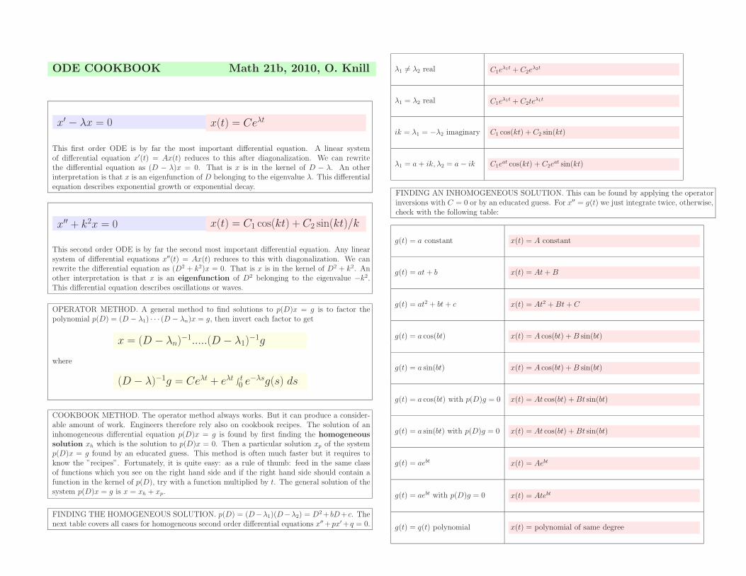
ODE COOKBOOK Math 21b, 2010, O. Knill

x′ − λx = 0 x(t) = Ceλt

This first order ODE is by far the most important differential equation. A linear systemof differential equation x′(t) = Ax(t) reduces to this after diagonalization. We can rewritethe differential equation as (D − λ)x = 0. That is x is in the kernel of D − λ. An otherinterpretation is that x is an eigenfunction of D belonging to the eigenvalue λ. This differentialequation describes exponential growth or exponential decay.

x′′ + k2x = 0 x(t) = C1 cos(kt) + C2 sin(kt)/k

This second order ODE is by far the second most important differential equation. Any linearsystem of differential equations x′′(t) = Ax(t) reduces to this with diagonalization. We canrewrite the differential equation as (D2 + k2)x = 0. That is x is in the kernel of D2 + k2. Another interpretation is that x is an eigenfunction of D2 belonging to the eigenvalue −k2.This differential equation describes oscillations or waves.

OPERATOR METHOD. A general method to find solutions to p(D)x = g is to factor thepolynomial p(D) = (D − λ1) · · · (D − λn)x = g, then invert each factor to get

x = (D − λn)−1.....(D − λ1)

−1g

where

(D − λ)−1g = Ceλt + eλt∫ t0 e

−λsg(s) ds

COOKBOOK METHOD. The operator method always works. But it can produce a consider-able amount of work. Engineers therefore rely also on cookbook recipes. The solution of aninhomogeneous differential equation p(D)x = g is found by first finding the homogeneous

solution xh which is the solution to p(D)x = 0. Then a particular solution xp of the systemp(D)x = g found by an educated guess. This method is often much faster but it requires toknow the ”recipes”. Fortunately, it is quite easy: as a rule of thumb: feed in the same classof functions which you see on the right hand side and if the right hand side should contain afunction in the kernel of p(D), try with a function multiplied by t. The general solution of thesystem p(D)x = g is x = xh + xp.

FINDING THE HOMOGENEOUS SOLUTION. p(D) = (D−λ1)(D−λ2) = D2+ bD+ c. Thenext table covers all cases for homogeneous second order differential equations x′′+px′+ q = 0.

λ1 6= λ2 real C1eλ1t + C2e

λ2t

λ1 = λ2 real C1eλ1t + C2te

λ1t

ik = λ1 = −λ2 imaginary C1 cos(kt) + C2 sin(kt)

λ1 = a + ik, λ2 = a− ik C1eat cos(kt) + C2e

at sin(kt)

FINDING AN INHOMOGENEOUS SOLUTION. This can be found by applying the operatorinversions with C = 0 or by an educated guess. For x′′ = g(t) we just integrate twice, otherwise,check with the following table:

g(t) = a constant x(t) = A constant

g(t) = at + b x(t) = At+B

g(t) = at2 + bt + c x(t) = At2 +Bt + C

g(t) = a cos(bt) x(t) = A cos(bt) +B sin(bt)

g(t) = a sin(bt) x(t) = A cos(bt) +B sin(bt)

g(t) = a cos(bt) with p(D)g = 0 x(t) = At cos(bt) +Bt sin(bt)

g(t) = a sin(bt) with p(D)g = 0 x(t) = At cos(bt) +Bt sin(bt)

g(t) = aebt x(t) = Aebt

g(t) = aebt with p(D)g = 0 x(t) = Atebt

g(t) = q(t) polynomial x(t) = polynomial of same degree

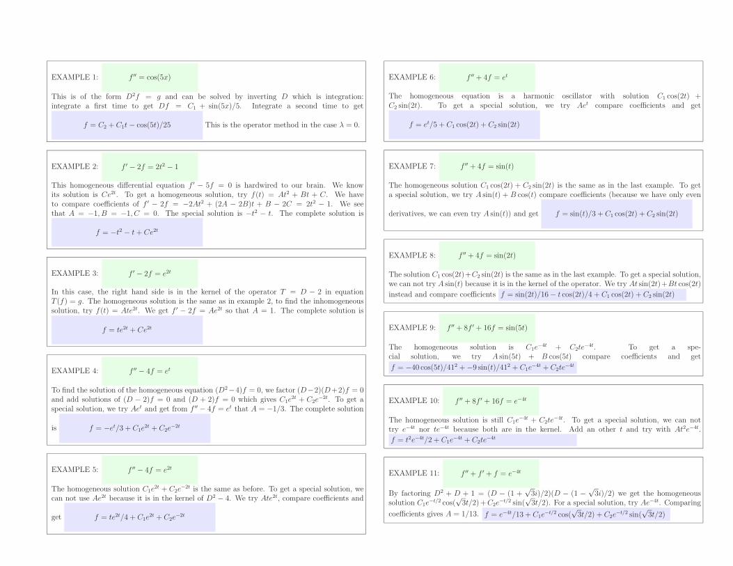
EXAMPLE 1: f ′′ = cos(5x)

This is of the form D2f = g and can be solved by inverting D which is integration:integrate a first time to get Df = C1 + sin(5x)/5. Integrate a second time to get

f = C2 + C1t− cos(5t)/25 This is the operator method in the case λ = 0.

EXAMPLE 2: f ′ − 2f = 2t2 − 1

This homogeneous differential equation f ′ − 5f = 0 is hardwired to our brain. We knowits solution is Ce2t. To get a homogeneous solution, try f(t) = At2 + Bt + C. We haveto compare coefficients of f ′ − 2f = −2At2 + (2A − 2B)t + B − 2C = 2t2 − 1. We seethat A = −1, B = −1, C = 0. The special solution is −t2 − t. The complete solution is

f = −t2 − t+ Ce2t

EXAMPLE 3: f ′ − 2f = e2t

In this case, the right hand side is in the kernel of the operator T = D − 2 in equationT (f) = g. The homogeneous solution is the same as in example 2, to find the inhomogeneoussolution, try f(t) = Ate2t. We get f ′ − 2f = Ae2t so that A = 1. The complete solution is

f = te2t + Ce2t

EXAMPLE 4: f ′′ − 4f = et

To find the solution of the homogeneous equation (D2−4)f = 0, we factor (D−2)(D+2)f = 0and add solutions of (D − 2)f = 0 and (D + 2)f = 0 which gives C1e

2t + C2e−2t. To get a

special solution, we try Aet and get from f ′′ − 4f = et that A = −1/3. The complete solution

is f = −et/3 + C1e2t + C2e

−2t

EXAMPLE 5: f ′′ − 4f = e2t

The homogeneous solution C1e2t + C2e

−2t is the same as before. To get a special solution, wecan not use Ae2t because it is in the kernel of D2 − 4. We try Ate2t, compare coefficients and

get f = te2t/4 + C1e2t + C2e

−2t

EXAMPLE 6: f ′′ + 4f = et

The homogeneous equation is a harmonic oscillator with solution C1 cos(2t) +C2 sin(2t). To get a special solution, we try Aet compare coefficients and get

f = et/5 + C1 cos(2t) + C2 sin(2t)

EXAMPLE 7: f ′′ + 4f = sin(t)

The homogeneous solution C1 cos(2t) + C2 sin(2t) is the same as in the last example. To geta special solution, we try A sin(t) + B cos(t) compare coefficients (because we have only even

derivatives, we can even try A sin(t)) and get f = sin(t)/3 + C1 cos(2t) + C2 sin(2t)

EXAMPLE 8: f ′′ + 4f = sin(2t)

The solution C1 cos(2t)+C2 sin(2t) is the same as in the last example. To get a special solution,we can not try A sin(t) because it is in the kernel of the operator. We try At sin(2t)+Bt cos(2t)

instead and compare coefficients f = sin(2t)/16− t cos(2t)/4 + C1 cos(2t) + C2 sin(2t)

EXAMPLE 9: f ′′ + 8f ′ + 16f = sin(5t)

The homogeneous solution is C1e−4t + C2te

−4t. To get a spe-cial solution, we try A sin(5t) + B cos(5t) compare coefficients and get

f = −40 cos(5t)/412 +−9 sin(t)/412 + C1e−4t + C2te

−4t

EXAMPLE 10: f ′′ + 8f ′ + 16f = e−4t

The homogeneous solution is still C1e−4t + C2te

−4t. To get a special solution, we can nottry e−4t nor te−4t because both are in the kernel. Add an other t and try with At2e−4t.

f = t2e−4t/2 + C1e−4t + C2te

−4t

EXAMPLE 11: f ′′ + f ′ + f = e−4t

By factoring D2 + D + 1 = (D − (1 +√3i)/2)(D − (1 −

√3i)/2) we get the homogeneous

solution C1e−t/2 cos(

√3t/2)+C2e

−t/2 sin(√3t/2). For a special solution, try Ae−4t. Comparing

coefficients gives A = 1/13. f = e−4t/13 + C1e−t/2 cos(

√3t/2) + C2e

−t/2 sin(√3t/2)

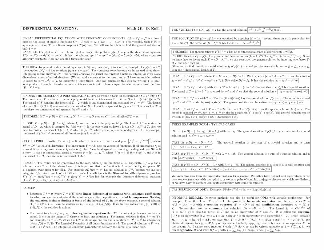
DIFFERENTIAL EQUATIONS, Math 21b, O. Knill

LINEAR DIFFERENTIAL EQUATIONS WITH CONSTANT COEFFICIENTS. Df = Tf = f ′ is a linearmap on the space of smooth functions C∞. If p(x) = a0 + a1x + ... + anx

n is a polynomial, then p(D) =a0 + a1D + ... + anD

n is a linear map on C∞(R) too. We will see here how to find the general solution ofp(D)f = g.EXAMPLE. For p(x) = x2

− x + 6 and g(x) = cos(x) the problem p(D)f = g is the differential equationf ′′(x) − f ′(x) − 6f(x) = cos(x). It has the solution c1e

−2x + c2e3x

− (sin(x) + 7 cos(x))/50, where c1, c2 arearbitrary constants. How can one find these solutions?

THE IDEA. In general, a differential equation p(D)f = g has many solution. For example, for p(D) = D3,the equation D3f = 0 has solutions (c0 + c1x+ c2x

2). The constants come because we integrated three times.Integrating means applying D−1 but because D has as the kernel the constant functions, integration gives a onedimensional space of anti-derivatives. (We can add a constant to the result and still have an anti-derivative).In order to solve D3f = g, we integrate g three times. One can generalize this idea by writing T = p(D)as a product of simpler transformations which we can invert. These simpler transformations have the form(D − λ)f = g.

FINDING THE KERNEL OFA POLYNOMIAL IN D. How do we find a basis for the kernel of Tf = f ′′+2f ′+f?The linear map T can be written as a polynomial in D which means T = D2

− D − 2 = (D + 1)(D − 2).The kernel of T contains the kernel of D − 2 which is one-dimensional and spanned by f1 = e2x. The kernelof T = (D − 2)(D + 1) also contains the kernel of D + 1 which is spanned by f2 = e−x. The kernel of T istherefore two dimensional and spanned by e2x and e−x.

THEOREM: If T = p(D) = Dn + an−1Dn−1 + ...+ a1D + a0 on C∞ then dim(ker(T )) = n.

PROOF. T = p(D) =∏

(D − λj), where λj are the roots of the polynomial p. The kernel of T contains thekernel of D − λj which is spanned by fj(t) = eλjt. In the case when we have a factor (D − λj)

k of T , then wehave to consider the kernel of (D− λj)

k which is q(t)eλt, where q is a polynomial of degree k− 1. For example,the kernel of (D − 1)3 consists of all functions (a+ bt+ ct2)et.

SECOND PROOF. Write this as Ag = 0, where A is a n × n matrix and g =[

f, f , · · · , f (n−1)]T

, where

f (k) = Dkf is the k’th derivative. The linear map T = AD acts on vectors of functions. If all eigenvalues λj ofA are different (they are the same λj as before), then A can be diagonalized. Solving the diagonal case BD = 0is easy. It has a n dimensional kernel of vectors F = [f1, . . . , fn]

T , where fi(t) = t. If B = SAS−1, and F is inthe kernel of BD, then SF is in the kernel of AD.

REMARK. The result can be generalized to the case, when aj are functions of x. Especially, Tf = g has asolution, when T is of the above form. It is important that the function in front of the highest power Dn

is bounded away from 0 for all t. For example xDf(x) = ex has no solution in C∞, because we can notintegrate ex/x. An example of a ODE with variable coefficients is the Sturm-Liouville eigenvalue problemT (f)(x) = a(x)f ′′(x) + a′(x)f ′(x) + q(x)f(x) = λf(x) like for example the Legendre differential equation(1− x2)f ′′(x) − 2xf ′(x) + n(n+ 1)f(x) = 0.

BACKUP

• Equations Tf = 0, where T = p(D) form linear differential equations with constant coefficients

for which we want to understand the solution space. Such equations are called homogeneous. Solvingthe equation includes finding a basis of the kernel of T . In the above example, a general solutionof f ′′ + 2f ′ + f = 0 can be written as f(t) = a1f1(t) + a2f2(t). If we fix two values like f(0), f ′(0) orf(0), f(1), the solution is unique.

• If we want to solve Tf = g, an inhomogeneous equation then T−1 is not unique because we have akernel. If g is in the image of T there is at least one solution f . The general solution is then f + ker(T ).For example, for T = D2, which has C∞ as its image, we can find a solution to D2f = t3 by integratingtwice: f(t) = t5/20. The kernel of T consists of all linear functions at+b. The general solution to D2 = t3

is at+ b+ t5/20. The integration constants parameterize actually the kernel of a linear map.

THE SYSTEM Tf = (D − λ)f = g has the general solution ceλx + eλx∫ x

0 e−λtg(t) dt .

THE SOLUTION OF (D − λ)kf = g is obtained by applying (D − λ)−1 several times on g. In particular, for

g = 0, we get the kernel of (D − λ)k as (c0 + c1x+ ...+ ck−1xk−1)eλx .

THEOREM. The inhomogeneous p(D)f = g has an n-dimensional space of solutions in C∞(R).

PROOF. To solve Tf = p(D)f = g, we write the equation as (D − λ1)k1(D − λ2)

k2· · · (D − λn)

knf = g. Sincewe know how to invert each Tj = (D − λj)

kj , we can construct the general solution by inverting one factor Tj

of T one after another.Often we can find directly a special solution f1 of p(D)f = g and get the general solution as f1 + fh, where fhis in the n-dimensional kernel of T .

EXAMPLE 1) Tf = e3x, where T = D2−D = D(D − 1). We first solve (D − 1)f = e3x. It has the solution

f1 = cex + ex∫ x

0e−te3t dt = c2e

x + e3x/2. Now solve Df = f1. It has the solution c1 + c2ex + e3x/6 .

EXAMPLE 2) Tf = sin(x) with T = (D2− 2D + 1) = (D − 1)2. We see that cos(x)/2 is a special solution.

The kernel of T = (D − 1)2 is spanned by xex and ex so that the general solution is (c1 + c2x)ex + cos(x)/2 .

EXAMPLE 3) Tf = x with T = D2+1 = (D−i)(D+i) has the special solution f(x) = x. The kernel is spanned

by eix and e−ix or also by cos(x), sin(x). The general solution can be written as c1 cos(x) + c2 sin(x) + x .

EXAMPLE 4) Tf = x with T = D4 + 2D2 + 1 = (D − i)2(D + i)2 has the special solution f(x) = x. Thekernel is spanned by eix, xeix, e−ix, x−ix or also by cos(x), sin(x), x cos(x), x sin(x). The general solution can be

written as (c0 + c1x) cos(x) + (d0 + d1x) sin(x) + x .

THESE EXAMPLES FORM 4 TYPICAL CASES.

CASE 1) p(D) = (D − λ1)...(D − λn) with real λi. The general solution of p(D)f = g is the sum of a special

solution and c1eλ1x + ...+ cne

λnx

CASE 2) p(D) = (D − λ)k. The general solution is the sum of a special solution and a term

(c0 + c1x+ ...+ ck−1xk−1)eλx

CASE 3) p(D) = (D − λ)(D − λ) with λ = a + ib. The general solution is a sum of a special solution and a

term c1eax cos(bx) + c2e

ax sin(bx)

CASE 4) p(D) = (D − λ)k(D − λ)k with λ = a + ib. The general solution is a sum of a special solution and

(c0 + c1x+ ...+ ck−1xk−1)eax cos(bx) + (d0 + d1x+ ...+ dk−1x

k−1)eax sin(bx)

We know this also from the eigenvalue problem for a matrix. We either have distinct real eigenvalues, or wehave some eigenvalues with multiplicity, or we have pairs of complex conjugate eigenvalues which are distinct,or we have pairs of complex conjugate eigenvalues with some multiplicity.

CAS SOLUTION OF ODE’s: Example: DSolve[f′′[x]− f′[x] == Exp[3x], f[x], x]

INFORMAL REMARK. Operator methods can also be useful for ODEs with variable coefficients. Forexample, T = H − 1 = D2

− x2− 1, the quantum harmonic oscillator, can be written as T =

A∗A = AA∗ + 2 with a creation operator A∗ = (D − x) and annihilation operator A = (D +

x). To see this, use the commutation relation Dx − xD = 1. The kernel f0 = Ce−x2/2 ofA = (D + x) is also the kernel of T and so an eigenvector of T and H . It is called the vacuum.

If f is an eigenvector of H with Hf = λf , then A∗f is an eigenvector with eigenvalue λ+ 2 . Proof. Because

HA∗− A∗H = [H,A∗] = 2A∗, we have H(A∗f) = A∗Hf + [H,A∗]f = A∗λf + 2A∗f = (λ + 2)(A∗f). We

obtain all eigenvectors fn = A∗fn−1 of eigenvalue 1 + 2n by applying iteratively the creation operator A∗ onthe vacuum f0. Because every function f with

∫

f2 dx < ∞ can be written uniquely as f =∑

∞

n=0 anfn, wecan diagonalize H and solve Hf = g with f =

∑

n bn/(1 + 2n)fn, where g =∑

n bnfn.

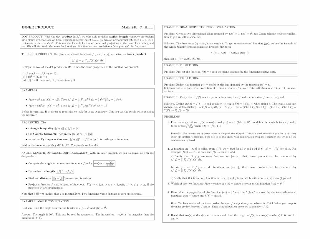
INNER PRODUCT Math 21b, O. Knill

DOT PRODUCT. With the dot product in Rn, we were able to define angles, length, compute projectionsonto planes or reflections on lines. Especially recall that if ~w1, ..., ~wn was an orthonormal set, then ~v = a1 ~w1 +... + an ~wn with ai = ~v · ~wi. This was the formula for the orthonormal projection in the case of an orthogonalset. We will aim to do the same for functions. But first we need to define a ”dot product” for functions.

THE INNER PRODUCT. For piecewise smooth functions f, g on [−π, π], we define the inner product

〈f, g〉 = 1

π

∫ π

−πf(x)g(x) dx

It plays the role of the dot product in Rn. It has the same properties as the familiar dot product:

(i) 〈f + g, h〉 = 〈f, h〉+ 〈g, h〉.(ii) ||f ||2 = 〈f, g〉 ≥ 0(iii) ||f ||2 = 0 if and only if f is identically 0

EXAMPLES.

• f(x) = x2 and g(x) =√x. Then 〈f, g〉 = 1

π

∫ π

−πx3/2 dx = 1

πx5/2 2

5|π−π = 4

5

√π3.

• f(x) = sin2(x), g(x) = x3. Then 〈f, g〉 = 1

π

∫ π

−π sin2(x)x3 dx = ...?

Before integrating, Ii is always a good idea to look for some symmetry. Can you see the result without doingthe integral?

PROPERTIES. The

• triangle inequality ||f + g|| ≤ ||f ||+ ||g|.

• the Cauchy-Schwartz inequality |〈f, g〉 ≤ ||f || ||g||

• as well as Pythagoras theorem ||f + g||2 = ||f ||2 + ||g||2 for orthogonal functions

hold in the same way as they did in Rn. The proofs are identical.

ANGLE, LENGTH, DISTANCE, ORTHOGONALITY. With an inner product, we can do things as with thedot product:

• Compute the angle α between two functions f and g cos(α) = 〈f,g〉||f ||·||g||

• Determine the length ||f ||2 = 〈f, f〉

• Find and distance ||f − g|| between two functions

• Project a function f onto a space of functions. P (f) =< f, g1 > g1+ < f, g2)g2...+ < f, gn > gn if thefunctions gi are orthonormal.

Note that ||f || = 0 implies that f is identically 0. Two functions whose distance is zero are identical.

EXAMPLE: ANGLE COMPUTATION.

Problem: Find the angle between the functions f(t) = t3 and g(t) = t4.

Answer: The angle is 90◦. This can be seen by symmetry. The integral on [−π, 0] is the negative then theintegral on [0, π].

EXAMPLE: GRAM SCHMIDT ORTHOGONALIZATION.

Problem: Given a two dimensional plane spanned by f1(t) = 1, f2(t) = t2, use Gram-Schmidt orthonormaliza-tion to get an orthonormal set.

Solution. The function g1(t) = 1/√2 has length 1. To get an orthonormal function g2(t), we use the formula of

the Gram-Schmidt orthogonalization process: first form

h2(t) = f2(t)− 〈f2(t), g1(t)〉g1(t)

then get g2(t) = h2(t)/||h2(t)||.

EXAMPLE: PROJECTION.

Problem: Project the function f(t) = t onto the plane spanned by the functions sin(t), cos(t).

EXAMPLE: REFLECTION.

Problem: Reflect the function f(t) = cos(t) at the line spanned by the function g(t) = t.Solution: Let c = ||g||. The projection of f onto g is h = 〈f, g〉g/c2. The reflection is f + 2(h − f) as withvectors.

EXAMPLE: Verify that if f(t) is a 2π periodic function, then f and its derivative f ′ are orthogonal.

Solution. Define g(x, t) = f(x + t) and consider its length l(t) = ||g(x, t)|| when fixing t. The length does notchange. So, differentiating 0 = l′(t) = d/dt〈f(x + t), f(x + t)〉 = 〈f ′(x + t), f(x + t)〉 + 〈f(x + t), f ′(x + t)〉 =2〈f ′(x+ t), f(x+ t)〉.

PROBLEMS.

1. Find the angle between f(x) = cos(x) and g(x) = x2. (Like in Rn, we define the angle between f and g

to be arccos 〈f,g〉‖f‖‖g‖ where ‖f‖ =

√

〈f, f〉.)

Remarks. Use integration by parts twice to compute the integral. This is a good exercise if you feel a bit rusty

about integration techniques. Feel free to double check your computation with the computer but try to do the

computation by hand.

2. A function on [−π, π] is called even if f(−x) = f(x) for all x and odd if f(−x) = −f(x) for all x. Forexample, f(x) = cosx is even and f(x) = sinx is odd.

a) Verify that if f, g are even functions on [−π, π], their inner product can be computed by〈f, g〉 = 2

π

∫ π

0f(x)g(x) dx.

b) Verify that if f, g are odd functions on [−π, π], their inner product can be computed by〈f, g〉 = 2

π

∫ π

0f(x)g(x) dx.

c) Verify that if f is an even function on [−π, π] and g is an odd function on [−π, π], then 〈f, g〉 = 0.

3. Which of the two functions f(x) = cos(x) or g(x) = sin(x) is closer to the function h(x) = x2?

4. Determine the projection of the function f(x) = x2 onto the ”plane” spanned by the two orthonormalfunctions g(x) = cos(x) and h(x) = sin(x).

Hint. You have computed the inner product between f and g already in problem 1). Think before you compute

the inner product between f and h. There is no calculation necessary to compute 〈f, h〉.

5. Recall that cos(x) and sin(x) are orthonormal. Find the length of f(x) = a cos(x) + b sin(x) in terms of aand b.

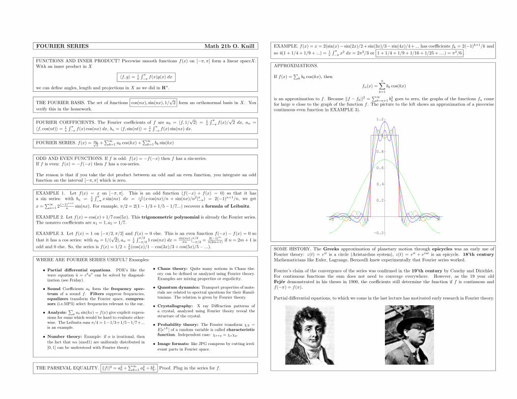
FOURIER SERIES Math 21b O. Knill

FUNCTIONS AND INNER PRODUCT? Piecewise smooth functions f(x) on [−π, π] form a linear spaceX .With an inner product in X

〈f, g〉 = 1π

∫ π

−πf(x)g(x) dx

we can define angles, length and projections in X as we did in Rn.

THE FOURIER BASIS. The set of functions cos(nx), sin(nx), 1/√2 form an orthonormal basis in X . You

verify this in the homework.

FOURIER COEFFICIENTS. The Fourier coefficients of f are a0 = 〈f, 1/√2〉 = 1

π

∫ π

−π f(x)/√2 dx, an =

〈f, cos(nt)〉 = 1π

∫ π

−π f(x) cos(nx) dx, bn = 〈f, sin(nt)〉 = 1π

∫ π

−π f(x) sin(nx) dx.

FOURIER SERIES. f(x) = a0√2+∑∞

k=1 ak cos(kx) +∑∞

k=1 bk sin(kx)

ODD AND EVEN FUNCTIONS. If f is odd: f(x) = −f(−x) then f has a sin-series.If f is even: f(x) = −f(−x) then f has a cos-series.

The reason is that if you take the dot product between an odd and an even function, you integrate an oddfunction on the interval [−π, π] which is zero.

EXAMPLE 1. Let f(x) = x on [−π, π]. This is an odd function (f(−x) + f(x) = 0) so that it hasa sin series: with bn = 1

π

∫ π

−π x sin(nx) dx = −1π (x cos(nx)/n + sin(nx)/n2|π−π) = 2(−1)n+1/n, we get

x =∑∞

n=1 2(−1)n+1

n sin(nx). For example, π/2 = 2(1− 1/3 + 1/5− 1/7...) recovers a formula of Leibnitz.

EXAMPLE 2. Let f(x) = cos(x)+1/7 cos(5x). This trigonometric polynomial is already the Fourier series.The nonzero coefficients are a1 = 1, a5 = 1/7.

EXAMPLE 3. Let f(x) = 1 on [−π/2, π/2] and f(x) = 0 else. This is an even function f(−x) − f(x) = 0 so

that it has a cos series: with a0 = 1/(√2), an = 1

π

∫ π/2

−π/21 cos(nx) dx = sin(nx)

πn |π/2−π/2 = 2(−1)m

π(2m+1) if n = 2m+ 1 is

odd and 0 else. So, the series is f(x) = 1/2 + 2π (cos(x)/1− cos(3x)/3 + cos(5x)/5− ...).

WHERE ARE FOURIER SERIES USEFUL? Examples:

• Partial differential equations. PDE’s like thewave equation u = c2u′′ can be solved by diagonal-ization (see Friday).

• Sound Coefficients ak form the frequency spec-

trum of a sound f . Filters suppress frequencies,equalizers transform the Fourier space, compres-

sors (i.e.MP3) select frequencies relevant to the ear.

• Analysis:∑

kak sin(kx) = f(x) give explicit expres-

sions for sums which would be hard to evaluate other-wise. The Leibnitz sum π/4 = 1−1/3+1/5−1/7+ ...is an example.

• Number theory: Example: if α is irrational, then

the fact that nα (mod1) are uniformly distributed in

[0, 1] can be understood with Fourier theory.

• Chaos theory: Quite many notions in Chaos the-ory can be defined or analyzed using Fourier theory.Examples are mixing properties or ergodicity.

• Quantum dynamics: Transport properties of mate-rials are related to spectral questions for their Hamil-tonians. The relation is given by Fourier theory.

• Crystallography: X ray Diffraction patterns ofa crystal, analyzed using Fourier theory reveal thestructure of the crystal.

• Probability theory: The Fourier transform χX =E[eiX ] of a random variable is called characteristic

function. Independent case: χx+y = χxχy.

• Image formats: like JPG compress by cutting irrel-

evant parts in Fourier space.

THE PARSEVAL EQUALITY. ||f ||2 = a20 +∑∞

k=1 a2k + b2k. Proof. Plug in the series for f .

EXAMPLE. f(x) = x = 2(sin(x)− sin(2x)/2+ sin(3x)/3− sin(4x)/4+ ... has coefficients fk = 2(−1)k+1/k and

so 4(1 + 1/4 + 1/9 + ...) = 1π

∫ π

−πx2 dx = 2π2/3 or 1 + 1/4 + 1/9 + 1/16 + 1/25 + ....) = π2/6 .

APPROXIMATIONS.

If f(x) =∑

k bk cos(kx), then

fn(x) =n∑

k=1

bk cos(kx)

is an approximation to f . Because ||f − fk||2 =∑∞

k=n+1 b2k goes to zero, the graphs of the functions fn come

for large n close to the graph of the function f . The picture to the left shows an approximation of a piecewisecontinuous even function in EXAMPLE 3).

-3 -2 -1 1 2 3

-0.2

0.2

0.4

0.6

0.8

1

1.2

SOME HISTORY. The Greeks approximation of planetary motion through epicycles was an early use ofFourier theory: z(t) = eit is a circle (Aristarchus system), z(t) = eit + eint is an epicycle. 18’th century

Mathematicians like Euler, Lagrange, Bernoulli knew experimentally that Fourier series worked.

Fourier’s claim of the convergence of the series was confirmed in the 19’th century by Cauchy and Dirichlet.For continuous functions the sum does not need to converge everywhere. However, as the 19 year oldFejer demonstrated in his theses in 1900, the coefficients still determine the function if f is continuous andf(−π) = f(π).

Partial differential equations, to which we come in the last lecture has motivated early research in Fourier theory.

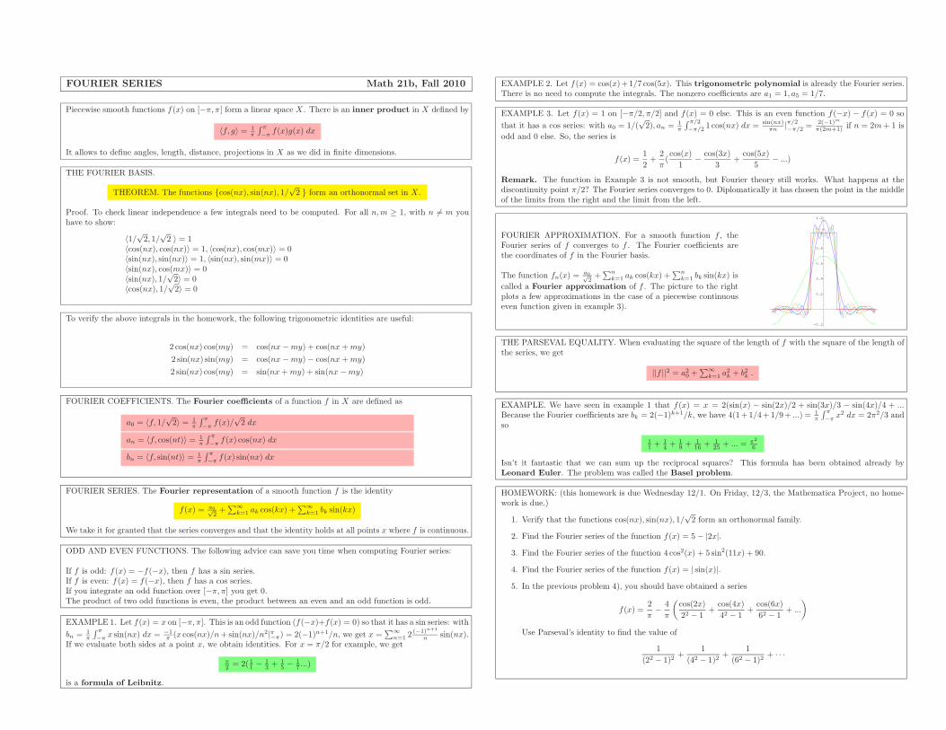
FOURIER SERIES Math 21b, Fall 2010

Piecewise smooth functions f(x) on [−π, π] form a linear space X . There is an inner product in X defined by

〈f, g〉 = 1π

∫ π

−π f(x)g(x) dx

It allows to define angles, length, distance, projections in X as we did in finite dimensions.

THE FOURIER BASIS.

THEOREM. The functions {cos(nx), sin(nx), 1/√2 } form an orthonormal set in X .

Proof. To check linear independence a few integrals need to be computed. For all n,m ≥ 1, with n 6= m youhave to show:

〈1/√2, 1/

√2 〉 = 1

〈cos(nx), cos(nx)〉 = 1, 〈cos(nx), cos(mx)〉 = 0〈sin(nx), sin(nx)〉 = 1, 〈sin(nx), sin(mx)〉 = 0〈sin(nx), cos(mx)〉 = 0〈sin(nx), 1/

√2〉 = 0

〈cos(nx), 1/√2〉 = 0

To verify the above integrals in the homework, the following trigonometric identities are useful:

2 cos(nx) cos(my) = cos(nx−my) + cos(nx+my)

2 sin(nx) sin(my) = cos(nx−my)− cos(nx+my)

2 sin(nx) cos(my) = sin(nx+my) + sin(nx−my)

FOURIER COEFFICIENTS. The Fourier coefficients of a function f in X are defined as

a0 = 〈f, 1/√2〉 = 1

π

∫ π

−πf(x)/

√2 dx

an = 〈f, cos(nt)〉 = 1π

∫ π

−π f(x) cos(nx) dx

bn = 〈f, sin(nt)〉 = 1π

∫ π

−πf(x) sin(nx) dx

FOURIER SERIES. The Fourier representation of a smooth function f is the identity

f(x) = a0√2+∑∞

k=1 ak cos(kx) +∑∞

k=1 bk sin(kx)

We take it for granted that the series converges and that the identity holds at all points x where f is continuous.

ODD AND EVEN FUNCTIONS. The following advice can save you time when computing Fourier series:

If f is odd: f(x) = −f(−x), then f has a sin series.If f is even: f(x) = f(−x), then f has a cos series.If you integrate an odd function over [−π, π] you get 0.The product of two odd functions is even, the product between an even and an odd function is odd.

EXAMPLE 1. Let f(x) = x on [−π, π]. This is an odd function (f(−x)+f(x) = 0) so that it has a sin series: with

bn = 1π

∫ π

−π x sin(nx) dx = −1π (x cos(nx)/n+sin(nx)/n2|π−π) = 2(−1)n+1/n, we get x =

∑∞n=1 2

(−1)n+1

n sin(nx).If we evaluate both sides at a point x, we obtain identities. For x = π/2 for example, we get

π2 = 2(11 − 1

3 + 15 − 1

7 ...)

is a formula of Leibnitz.

EXAMPLE 2. Let f(x) = cos(x)+1/7 cos(5x). This trigonometric polynomial is already the Fourier series.There is no need to compute the integrals. The nonzero coefficients are a1 = 1, a5 = 1/7.

EXAMPLE 3. Let f(x) = 1 on [−π/2, π/2] and f(x) = 0 else. This is an even function f(−x) − f(x) = 0 so

that it has a cos series: with a0 = 1/(√2), an = 1

π

∫ π/2

−π/2 1 cos(nx) dx = sin(nx)πn |π/2−π/2 = 2(−1)m

π(2m+1) if n = 2m+ 1 is

odd and 0 else. So, the series is

f(x) =1

2+

2

π(cos(x)

1− cos(3x)

3+

cos(5x)

5− ...)

Remark. The function in Example 3 is not smooth, but Fourier theory still works. What happens at thediscontinuity point π/2? The Fourier series converges to 0. Diplomatically it has chosen the point in the middleof the limits from the right and the limit from the left.

FOURIER APPROXIMATION. For a smooth function f , theFourier series of f converges to f . The Fourier coefficients arethe coordinates of f in the Fourier basis.

The function fn(x) =a0√2+∑n

k=1 ak cos(kx) +∑n

k=1 bk sin(kx) is

called a Fourier approximation of f . The picture to the rightplots a few approximations in the case of a piecewise continuouseven function given in example 3).

-3 -2 -1 1 2 3

-0.2

0.2

0.4

0.6

0.8

1

1.2

THE PARSEVAL EQUALITY. When evaluating the square of the length of f with the square of the length ofthe series, we get

||f ||2 = a20 +∑∞

k=1 a2k + b2k .

EXAMPLE. We have seen in example 1 that f(x) = x = 2(sin(x) − sin(2x)/2 + sin(3x)/3 − sin(4x)/4 + ...Because the Fourier coefficients are bk = 2(−1)k+1/k, we have 4(1+1/4+1/9+ ...) = 1

π

∫ π

−πx2 dx = 2π2/3 and

so

11 + 1

4 + 19 + 1

16 + 125 + ... = π2

6

Isn’t it fantastic that we can sum up the reciprocal squares? This formula has been obtained already byLeonard Euler. The problem was called the Basel problem.

HOMEWORK: (this homework is due Wednesday 12/1. On Friday, 12/3, the Mathematica Project, no home-work is due.)

1. Verify that the functions cos(nx), sin(nx), 1/√2 form an orthonormal family.

2. Find the Fourier series of the function f(x) = 5− |2x|.

3. Find the Fourier series of the function 4 cos2(x) + 5 sin2(11x) + 90.

4. Find the Fourier series of the function f(x) = | sin(x)|.

5. In the previous problem 4), you should have obtained a series

f(x) =2

π− 4

π

(

cos(2x)

22 − 1+

cos(4x)

42 − 1+

cos(6x)

62 − 1+ ...

)

Use Parseval’s identity to find the value of

1

(22 − 1)2+

1

(42 − 1)2+

1

(62 − 1)2+ · · ·

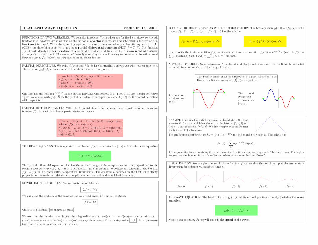
HEAT AND WAVE EQUATION Math 21b, Fall 2010

FUNCTIONS OF TWO VARIABLES. We consider functions f(x, t) which are for fixed t a piecewise smoothfunction in x. Analogously as we studied the motion of a vector ~v(t), we are now interested in the motion of afunction f in time t. While the governing equation for a vector was an ordinary differential equation x = Ax(ODE), the describing equation is now be a partial differential equation (PDE) f = T (f). The functionf(x, t) could denote the temperature of a stick at a position x at time t or the displacement of a string

at the position x at time t. The motion of these dynamical systems will be easy to describe in the orthonormalFourier basis 1/

√2, sin(nx), cos(nx) treated in an earlier lecture.

PARTIAL DERIVATIVES. We write fx(x, t) and ft(x, t) for the partial derivatives with respect to x or t.The notation fxx(x, t) means that we differentiate twice with respect to x.

Example: for f(x, t) = cos(x+ 4t2), we have• fx(x, t) = − sin(x+ 4t2)• ft(x, t) = −8t sin(x+ 4t2).• fxx(x, t) = − cos(x+ 4t2).

One also uses the notation ∂f(x,y)∂x for the partial derivative with respect to x. Tired of all the ”partial derivative

signs”, we always write fx(x, t) for the partial derivative with respect to x and ft(x, t) for the partial derivativewith respect to t.

PARTIAL DIFFERENTIAL EQUATIONS. A partial differential equation is an equation for an unknownfunction f(x, t) in which different partial derivatives occur.

• ft(x, t) + fx(x, t) = 0 with f(x, 0) = sin(x) has asolution f(x, t) = sin(x− t).• ftt(x, t) − fxx(x, t) = 0 with f(x, 0) = sin(x) andft(x, 0) = 0 has a solution f(x, t) = (sin(x − t) +sin(x+ t))/2.

THE HEAT EQUATION. The temperature distribution f(x, t) in a metal bar [0, π] satisfies the heat equation

ft(x, t) = µfxx(x, t)

This partial differential equation tells that the rate of change of the temperature at x is proportional to thesecond space derivative of f(x, t) at x. The function f(x, t) is assumed to be zero at both ends of the bar andf(x) = f(x, t) is a given initial temperature distribution. The constant µ depends on the heat conductivityproperties of the material. Metals for example conduct heat well and would lead to a large µ.

REWRITING THE PROBLEM. We can write the problem as

ddtf = µD2f

We will solve the problem in the same way as we solved linear differential equations:

ddt~x = A~x

where A is a matrix - by diagonalization .

We use that the Fourier basis is just the diagonalization: D2 cos(nx) = (−n2) cos(nx) and D2 sin(nx) =

(−n2) sin(nx) show that cos(nx) and sin(nx) are eigenfunctions to D2 with eigenvalue −n2 . By a symmetrytrick, we can focus on sin-series from now on.

SOLVING THE HEAT EQUATION WITH FOURIER THEORY. The heat equation ft(x, t) = µfxx(x, t) withsmooth f(x, 0) = f(x), f(0, t) = f(π, t) = 0 has the solution

f(x, t) =∑∞

n=1 bn sin(nx)e−n2µt bn = 2

π

∫ π

0f(x) sin(nx) dx

Proof: With the initial condition f(x) = sin(nx), we have the evolution f(x, t) = e−µn2t sin(nx). If f(x) =∑∞

n=1 bn sin(nx) then f(x, t) =∑∞

n=1 bne−µn2t sin(nx).

A SYMMETRY TRICK. Given a function f on the interval [0, π] which is zero at 0 and π. It can be extendedto an odd function on the doubled integral [−π, π].

The Fourier series of an odd function is a pure sin-series. TheFourier coefficients are bn = 2

π

∫ π

0 f(x) sin(nx) dx.

The functionis given on[0, π].

The oddsymmetricextension on[−π, π].

EXAMPLE. Assume the initial temperature distribution f(x, 0) isa sawtooth function which has slope 1 on the interval [0, π/2] andslope −1 on the interval [π/2, π]. We first compute the sin-Fouriercoefficients of this function.

The sin-Fourier coefficients are bn = 4n2π (−1)(n−1)/2 for odd n and 0 for even n. The solution is

f(x, t) =∞∑

n

bne−µn2t sin(nx) .

The exponential term containing the time makes the function f(x, t) converge to 0: The body cools. The higherfrequencies are damped faster: ”smaller disturbances are smoothed out faster.”

VISUALIZATION. We can plot the graph of the function f(x, t) or slice this graph and plot the temperaturedistribution for different values of the time t.

f(x, 0) f(x, 1) f(x, 2) f(x, 3) f(x, 4)

THE WAVE EQUATION. The height of a string f(x, t) at time t and position x on [0, π] satisfies the wave

equation

ftt(t, x) = c2fxx(t, x)

where c is a constant. As we will see, c is the speed of the waves.

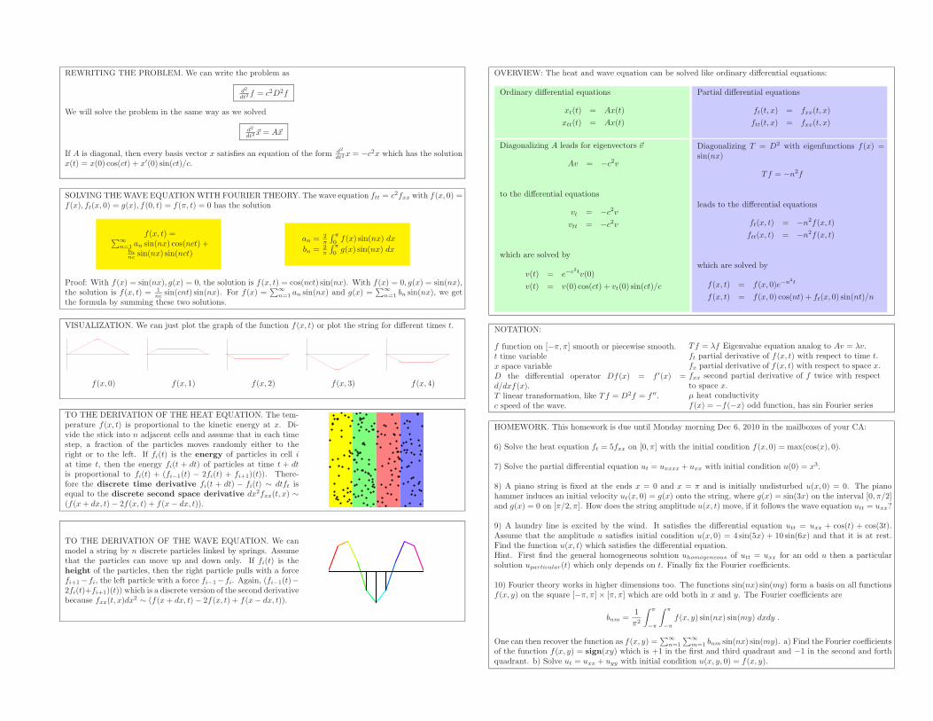
REWRITING THE PROBLEM. We can write the problem as

d2

dt2 f = c2D2f

We will solve the problem in the same way as we solved

d2

dt2 ~x = A~x

If A is diagonal, then every basis vector x satisfies an equation of the form d2

dt2x = −c2x which has the solutionx(t) = x(0) cos(ct) + x′(0) sin(ct)/c.

SOLVING THEWAVE EQUATIONWITH FOURIER THEORY. The wave equation ftt = c2fxx with f(x, 0) =f(x), ft(x, 0) = g(x), f(0, t) = f(π, t) = 0 has the solution

f(x, t) =∑∞

n=1 an sin(nx) cos(nct) +bnnc sin(nx) sin(nct)

an = 2π

∫ π

0f(x) sin(nx) dx

bn = 2π

∫ π

0g(x) sin(nx) dx

Proof: With f(x) = sin(nx), g(x) = 0, the solution is f(x, t) = cos(nct) sin(nx). With f(x) = 0, g(x) = sin(nx),the solution is f(x, t) = 1

nc sin(cnt) sin(nx). For f(x) =∑∞

n=1 an sin(nx) and g(x) =∑∞

n=1 bn sin(nx), we getthe formula by summing these two solutions.

VISUALIZATION. We can just plot the graph of the function f(x, t) or plot the string for different times t.

f(x, 0) f(x, 1) f(x, 2) f(x, 3) f(x, 4)

TO THE DERIVATION OF THE HEAT EQUATION. The tem-perature f(x, t) is proportional to the kinetic energy at x. Di-vide the stick into n adjacent cells and assume that in each timestep, a fraction of the particles moves randomly either to theright or to the left. If fi(t) is the energy of particles in cell iat time t, then the energy fi(t + dt) of particles at time t + dtis proportional to fi(t) + (fi−1(t) − 2fi(t) + fi+1)(t)). There-fore the discrete time derivative fi(t + dt) − fi(t) ∼ dtft isequal to the discrete second space derivative dx2fxx(t, x) ∼(f(x+ dx, t)− 2f(x, t) + f(x− dx, t)).

TO THE DERIVATION OF THE WAVE EQUATION. We canmodel a string by n discrete particles linked by springs. Assumethat the particles can move up and down only. If fi(t) is theheight of the particles, then the right particle pulls with a forcefi+1−fi, the left particle with a force fi−1−fi. Again, (fi−1(t)−2fi(t)+fi+1)(t)) which is a discrete version of the second derivativebecause fxx(t, x)dx

2 ∼ (f(x+ dx, t)− 2f(x, t) + f(x− dx, t)).

OVERVIEW: The heat and wave equation can be solved like ordinary differential equations:

Ordinary differential equations

xt(t) = Ax(t)

xtt(t) = Ax(t)

Partial differential equations

ft(t, x) = fxx(t, x)

ftt(t, x) = fxx(t, x)

Diagonalizing A leads for eigenvectors ~v

Av = −c2v

to the differential equations

vt = −c2v

vtt = −c2v

which are solved by

v(t) = e−c2tv(0)

v(t) = v(0) cos(ct) + vt(0) sin(ct)/c

Diagonalizing T = D2 with eigenfunctions f(x) =sin(nx)

Tf = −n2f

leads to the differential equations

ft(x, t) = −n2f(x, t)

ftt(x, t) = −n2f(x, t)

which are solved by

f(x, t) = f(x, 0)e−n2t

f(x, t) = f(x, 0) cos(nt) + ft(x, 0) sin(nt)/n

NOTATION:

f function on [−π, π] smooth or piecewise smooth.t time variablex space variableD the differential operator Df(x) = f ′(x) =d/dxf(x).T linear transformation, like Tf = D2f = f ′′.c speed of the wave.

Tf = λf Eigenvalue equation analog to Av = λv.ft partial derivative of f(x, t) with respect to time t.fx partial derivative of f(x, t) with respect to space x.fxx second partial derivative of f twice with respectto space x.µ heat conductivityf(x) = −f(−x) odd function, has sin Fourier series

HOMEWORK. This homework is due until Monday morning Dec 6, 2010 in the mailboxes of your CA:

6) Solve the heat equation ft = 5fxx on [0, π] with the initial condition f(x, 0) = max(cos(x), 0).

7) Solve the partial differential equation ut = uxxxx + uxx with initial condition u(0) = x3.

8) A piano string is fixed at the ends x = 0 and x = π and is initially undisturbed u(x, 0) = 0. The pianohammer induces an initial velocity ut(x, 0) = g(x) onto the string, where g(x) = sin(3x) on the interval [0, π/2]and g(x) = 0 on [π/2, π]. How does the string amplitude u(x, t) move, if it follows the wave equation utt = uxx?

9) A laundry line is excited by the wind. It satisfies the differential equation utt = uxx + cos(t) + cos(3t).Assume that the amplitude u satisfies initial condition u(x, 0) = 4 sin(5x) + 10 sin(6x) and that it is at rest.Find the function u(x, t) which satisfies the differential equation.Hint. First find the general homogeneous solution uhomogeneous of utt = uxx for an odd u then a particularsolution uparticular(t) which only depends on t. Finally fix the Fourier coefficients.

10) Fourier theory works in higher dimensions too. The functions sin(nx) sin(my) form a basis on all functionsf(x, y) on the square [−π, π]× [π, π] which are odd both in x and y. The Fourier coefficients are

bnm =1

π2

∫ π

−π

∫ π

−π

f(x, y) sin(nx) sin(my) dxdy .

One can then recover the function as f(x, y) =∑∞

n=1

∑∞m=1 bnm sin(nx) sin(my). a) Find the Fourier coefficients

of the function f(x, y) = sign(xy) which is +1 in the first and third quadrant and −1 in the second and forthquadrant. b) Solve ut = uxx + uyy with initial condition u(x, y, 0) = f(x, y).

MATH21BSYLLABUS 2010

Linear Algebra and Differential Equations is an introduction to linear algebra, including linear transformations, determinants, eigenvectors, eigenvalues, inner products and linear spaces. As for applications, the course introduces discrete dynamical systems and provides a solid introduction to differential equations, Fourier series as well as some partial differential equations. Other highlights include applications in statistics like Markov chains and data fitting with arbitrary functions.

Part Grade 1 Grade 2

1. Hourly 20 20

2. Hourly 20 20

Homework 20 20

Lab 5

Final 35 40

INtro 1.Exam 2.Exam

1. Sept 7. Oct 4. Nov

8:30 AM 7 PM 7 PM

SCB SCD SCD

† GRADES ¢

† IMPORTANT DATES ¢

† TEXTBOOK ¢

† ORGANIZATION ¢

Book: Otto Bretscher, Linear Algebra with Applications, 4th edition 2009,

ISBN-13:978-0-13-600926-9. You need the 4th edition for the homework. A student solution manual is optional.

† SECTIONING ¢

Course Head: Oliver Knill

knill@math.harvard.edu

SC 434, Tel: (617) 495 5549

More details:

http://www.math.harvard.edu/sectioning

† SECTIONS ¢

Course lectures (except reviews and intro meetings) are taught in sections. Sections: MWF 10,11,12.

† MQC ¢

Mathematics Question Center

† PROBLEM SESSIONS ¢

Run by course assistants

† PREREQUISITES ¢

Single variable calculus. Multivariable like 21a is advantage.

Start End Sent

Mo Jan 25 Wed Jan 27 Fri Jan 29

7 AM 12 PM 5 PM

Day to Day Syllabus

Su Mo Tu We Th Fr Sa

29 30 31 1 2 3 4

5 6 7 8 9 10 11

12 13 14 15 16 17 18

19 20 21 22 23 24 25

26 27 28 29 30 1 2

3 4 5 6 7 8 9

10 11 12 13 14 15 16

17 18 19 20 21 22 23

24 25 26 27 28 29 30

31 1 2 3 4 5 6

7 8 9 10 11 12 13

14 15 16 17 18 19 20

21 22 23 24 25 26 27

28 29 30 1 2 3 4

5 6 7 8 9 10 11

12 13 14 15 15 16 17

19 20 21 22 23 24 25

1. Week: Systems of linear equations

Lect 1 9/8 1.1 introduction to linear systems

Lect 2 9/10 1.2 matrices , GaussJordan elimination

2. Week: Linear transformations

Lect 3 9/13 1.3 on solutions of linear systems

Lect 4 2/15 2.1 linear transformations and inverses

Lect 5 2/17 2.2 linear transformations in geometry

3. Week: Linear subspaces

Lect 6 9/20 2.3 matrix products

Lect 7 9/22 2.4 the inverse

Lect 8 2/24 3.1 image and kernel

4. Week: Dimension and coordinate change

Lect 9 9/27 3.2 bases and linear independence

Lect 10 2/29 3.3 dimension

Lect 11 10/1 3.4 change of coordinates

5. Week: Orthogonal projections

Lect 12 10/4 4.1 linear spaces

Lect 13 10/6 review for first midterm

Lect 14 10/8 5.1 orthonormal bases projections

6. Week: Orthogonality

Columbus day

Lect 15 10/13 5.2 Gram-Schmidt and QR

Lect 16 10/15 5.3 orthogonal transformations

7. Week: Determinants

Lect 17 10/18 5.4 least squares and data fitting

Lect 18 10/20 6.1 determinants 1

Lect 19 10/22 6.2 determinants 2

8. Week: Diagonalization

Lect 20 10/25 7.1-2 eigenvalues

Lect 21 10/27 7.3 eigenvectors

Lect 22 10/29 7.4 diagonalization

9. Week: Stability and symmetric matrices

Lect 23 11/1 7.5 complex eigenvalues

Lect 24 11/3 review for second midterm

Lect 25 11/5 7.6 stability

10. Week: Differential equations (ODE)

Lect 26 11/8 8.1 symmetric matrices

Lect 27 11/10 9.1 differential equations I

Lect 28 11/12 9.2 differential equations II

11. Week: Function spaces

Lect 29 11/15 9.4 nonlinear systems

Lect 30 11/17 4.2 trafos on function spaces

Lect 31 11/19 9.3 inhomogeneous ODE's I

12. Week: Inner product spaces

Lect 32 11/22 9.3 inhomogeneous ODE's II

Lect 33 11/24 5.5 inner product spaces

Thanksgiving

13. Week: Partial differential equations

Lect 34 11/29 Fourier theory I

Lect 35 12/1 Fourier II and PDE's

Lect 36 12/3 Partial differential equations

Calendar

http://www.courses.fas.harvard.edu/~math21b

Mathematica Pointers Math 21b, 2009 O. Knill

1. Installation

1. Get the software, 2. install, 3. note the machine ID, 4. request a password�

http :// r e g i s t e r . wolfram . com .� �

You will need the:�

Licence Number L2482−2405� �

You need Mathematica 7 to see all the features of the lab. Here is the FAS download link:�

http :// downloads . f a s . harvard . edu/download� �

You can download the assignment here:�

http ://www. cou r s e s . f a s . harvard . edu/˜math21b/ lab . html� �

2. Getting started

Cells: click into cell, hold down shift, then type return to evaluate a cell.Lists: are central in Mathematica�

{1 ,3 ,4 ,6}� �

is a list of numbers.�

s=Table [ Plot [ Cos [ n x ] , { x,−Pi ,Pi } ] ,{n , 1 , 1 0} ]Show [GraphicsArray [ s ] ]� �

defines and plots a list of graphs.�

Plot [Table [ Cos [ n x ] , {n , 1 , 1 0} ] , { x,−Pi ,Pi } ]� �

Functions: You can define functions of essentially everything.�

f [ n ] :=Table [Random [ ] , { n} ,{n } ]� �

for example produces a random n× n matrix.�

T[ f ] :=Play [ f [ x ] , { x , 0 , 1 } ] ; T[ Sin [ 10000 #] &]� �

Variables: If a variable is reused, this can lead to interferences. To clear all variables, use�

ClearAll [ ”Global ‘∗ ” ] ;� �

Equality: there are two different equal signs. Think about = as =! and == as =?.�

a=4;a==2+2;� �

Objects: Mathematica is extremely object oriented. Objects can be movies, sound, func-tions, transformations etc.

3. The interface

The menu: Evaluation: abort to stop processesLook up: Help pages in the program, Google for a command.Websites: Wolfram demonstration project at http://demonstrations.wolfram.com/

4. The assignment

Walk through: There is example code for all assignments.

Problem 1) Plot the distribution of the eigenvalues of a random matrix, where each entryis a random number in [−0.4, 0.6].

Problem 2) Find the solution of the ordinary differential equation f ′′[x] + f ′[x] + f [x] ==Cos[x] + x4 with initial conditions f [0] == 1; f ′[0] == 0.

Problem 3) Find the Fourier series of the function f [x] := x7 on [−Pi, P i]. You need atleast 20 coefficients of the Fourier series.

Problem 4) Fit the prime numbers data = Table[k, Prime[k]/k], k, 100000] with functions1, x, Log[x]. The result will be a function. The result will suggest a growth rate of the primenumbers which is called the prime number theorem.

Problem 5) Freestyle: anything goes here. Nothing can be wrong. You can modify anyof the above examples a bit to write a little music tune or poem or try out some imagemanipulation function. It can be very remotely related to linear algebra.

Highlights: autotune, movie morphisms, random music and poems, statistics of determi-nants.The 5 problems: 4 structured problems, one free style

5. Some hints and tricks

�

?Eigen ∗� ��

Options [Det ]� �

Semicolons: important for display.Variables: don’t overload.

6. Questions and answer

The sky is the limitCaveats: Memory, CPU processes, blackbox.