Household Composition and Food Expenditures in China · 2002-09-10 · Household Composition and Food Expenditures in China Brian W. Gould Wisconsin Center for Dairy Research and

Household Composition and Food Expendituresin China

Brian W. GouldWisconsin Center for Dairy Research and Department of Agriculturaland Applied Economics, University of Wisconsin-Madison

ABSTRACT

With China admitted to the World Trade Organization there is the potential for dramatic increasesin U+S+ agricultural exports+ The present analysis uses household-level data to identify importantdeterminants of expenditures on food for at-home consumption by households in three Chineseurban provinces+ Besides the role of household income, we examine the impact of household mem-ber age0gender composition on expenditures via the estimation of endogenously determined adultequivalents+ Results from the analysis show that overall food at-home expenditures are incomeinelastic, some commodities exhibit elastic responses to changes in their own price and householdcomposition has a significant impact on food choice+ @JEL category: D120# + © 2002 Wiley Peri-odicals, Inc+

1. INTRODUCTION

With China admitted to the World Trade Organization there is the potential for dramaticincreases in U+S+ agricultural exports+ For example, USDA’s Foreign Agricultural Serviceestimates that China’s participation in the World Trade Organization would result in sub-stantial reductions in trade barriers and in an increase of at least $2 billion per year inagricultural exports by 2005 with exports of grains, oilseeds, and related products andcotton, alone projected to increase by $1+6 billion ~Colby, Price, & Tuan, 2000!+ Not onlywould tariffs be reduced significantly for poultry, pork, beef, fruits, forestry, and fishproducts there may also be significant reductions in a variety of non-tariff barriers for anumber of agricultural commodities ~USDA, 2000a!+

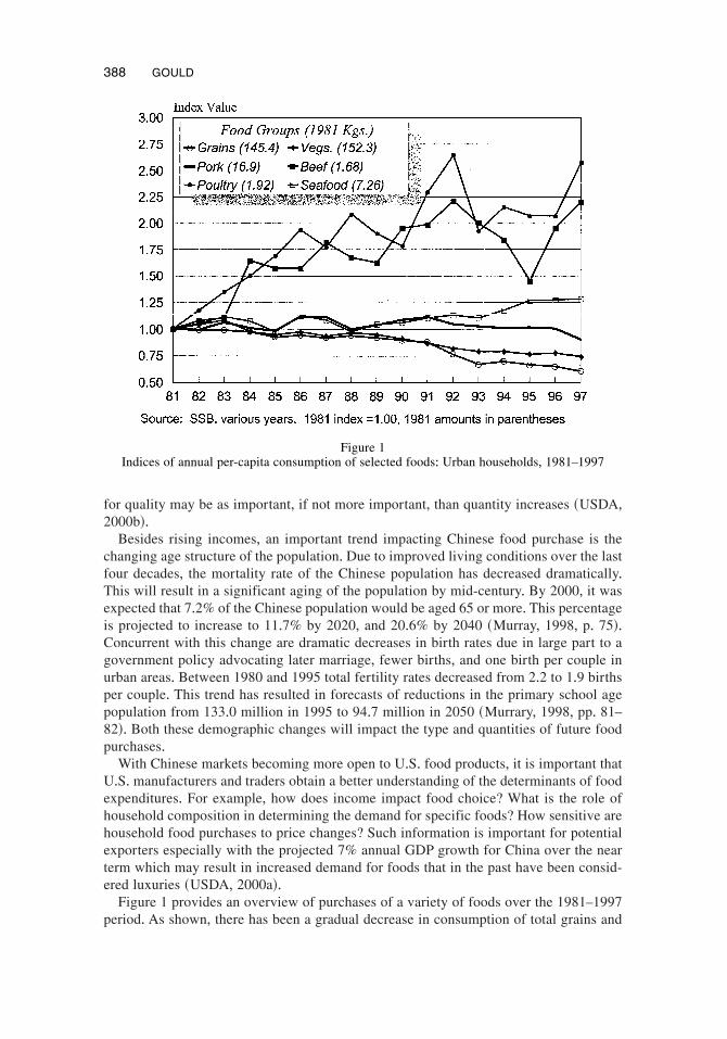
As China develops, there is general consensus that there will be an associated changein the Chinese diet ~Gao, Wailes, & Cramer, 1996!+ With rising incomes it is projectedthat the Chinese population will diversify their diets away from their dependence on sta-ples of rice and wheat flour, to one which contains more livestock products+ Using theexample of other Asian economies such as Japan, Korea, Hong Kong, and Singapore,most believe that consumption of beef will increase ~Shono, Suzuki, & Kaiser, 2000!+Currently, beef represents a small proportion of total meat products consumed but it hasbeen increasing in importance over the last two decades ~Fig+ 1!+ A desire for diversitywith higher incomes will likely lead to more rapid increases in beef consumption at theexpense of pork+Also, the beef currently consumed is of low quality+ Increases in demand

Agribusiness, Vol. 18 (3) 387–407 (2002) © 2002 Wiley Periodicals, Inc.Published online in Wiley InterScience (www.interscience.wiley.com). DOI: 10.1002/agr.10020

387

for quality may be as important, if not more important, than quantity increases ~USDA,2000b!+

Besides rising incomes, an important trend impacting Chinese food purchase is thechanging age structure of the population+ Due to improved living conditions over the lastfour decades, the mortality rate of the Chinese population has decreased dramatically+This will result in a significant aging of the population by mid-century+ By 2000, it wasexpected that 7+2% of the Chinese population would be aged 65 or more+ This percentageis projected to increase to 11+7% by 2020, and 20+6% by 2040 ~Murray, 1998, p+ 75!+Concurrent with this change are dramatic decreases in birth rates due in large part to agovernment policy advocating later marriage, fewer births, and one birth per couple inurban areas+ Between 1980 and 1995 total fertility rates decreased from 2+2 to 1+9 birthsper couple+ This trend has resulted in forecasts of reductions in the primary school agepopulation from 133+0 million in 1995 to 94+7 million in 2050 ~Murrary, 1998, pp+ 81–82!+ Both these demographic changes will impact the type and quantities of future foodpurchases+

With Chinese markets becoming more open to U+S+ food products, it is important thatU+S+ manufacturers and traders obtain a better understanding of the determinants of foodexpenditures+ For example, how does income impact food choice? What is the role ofhousehold composition in determining the demand for specific foods? How sensitive arehousehold food purchases to price changes? Such information is important for potentialexporters especially with the projected 7% annual GDP growth for China over the nearterm which may result in increased demand for foods that in the past have been consid-ered luxuries ~USDA, 2000a!+

Figure 1 provides an overview of purchases of a variety of foods over the 1981–1997period+ As shown, there has been a gradual decrease in consumption of total grains and

Figure 1Indices of annual per-capita consumption of selected foods: Urban households, 1981–1997

388 GOULD

vegetables, relatively stable pork and seafood consumption, and an increase in beef andpoultry purchases+ The data shown in this figure were obtained by dividing total house-hold food purchases by the number of household members+ This method of standardiza-tion does not take into account individual differences in food consumption needs+ Forexample, it does not recognize that the consumption needs of children can typically bemet at lower cost than that of adults ~Dreze and Srinivasan, 1997!+ The use in empiricaldemand analysis of a single household count variable as a deflator of food expendituresor its use as an explanatory variable is common practice+ It is important to remember thatsuch use incorporates the implicit assumption of the uniform impacts on expenditures ofhousehold members of different age and gender+

One approach that can be used to avoid the assumption of equal expenditure impacts isthe use of endogenously determined equivalence scales which assign different weights tohousehold members according to their age and gender ~Deaton and Muellbauer, 1986!+1

Given the determination of an appropriate equivalence scale, a comparison of food ex-penditures for households of differing composition can be undertaken+ For example, sup-pose the weight given to a male adult between 25 and 45 years of age is 1+0, a femaleadult in the same age group a weight of +85 and a female child under 10 years of age aweight of +35, then a four-member household consisting of one male and two femaleadults and one female child in the above age groups would result in the household beingcomposed of 3+05 adult equivalents+ A single parent household with one female adultwould possess the corresponding adult equivalent of 1+20+ The per capita expenditurespatterns of these two households can then be compared when the number of adult equiv-alents are used as the expenditure deflator+

Given the recognition of the need to obtain estimates of food adult equivalents to allowfor cross-household expenditure comparison, there are a number of approaches that havebeen suggested for the estimation of endogenously determined adult equivalent scales+These have ranged from the use of demographically translated utility consistent demandsystems to more ad hoc single equation approaches ~Muelbauer, 1980!+ Here, we use ademand system approach in an analysis of at-home food purchases by urban Chinesehouseholds over the 1995–1997 period+We adopt a method where the prices are scaled insuch a manner that a single household food equivalent is estimated for each householdusing an adult equivalent definition provided by Tedford, Capps, and Havlicek ~1986!+This is in contrast to previous analyses where food-specific scaling functions have beenestimated ~Gould, Cox, & Perali, 1991!+ Results of this analysis provide useful informa-tion to potential food exporters as to the market impacts of continued improvements inthe level of Chinese income and changing household composition+

Our analysis improves upon previous studies in that they have either not included de-mographic variables, have used a simple head count of household members as a measureof household size implying the same marginal impact on food expenditures, have notincluded price effects on purchase, or have not allowed for the effects of substitutability0complementarity with purchases of other food categories ~Gao,Wailes, & Cramer, 1996;Guo et al+, 2000; Halbrandt et al+, 1994;Wang & Chern, 1992!+

1When applied to an analysis of household income, adult equivalence scales are employed to adjust house-hold budgets to permit welfare comparisons across different size and composition+ That is, these scales are usedto account for the role of household size and composition in the transformation of income into welfare+ For areview of the methodological issues involved with the estimation of adult equivalence scales for welfare eval-uation refer to Blaylock ~1991!+

EXPENDITURES IN CHINA 389

2. DESCRIPTION OF THE ECONOMETRIC MODEL

For this analysis we assume that household at-home food demand is separable from thedemand from other goods+ Additionally, we assume that utility obtained from at-homefood purchases can be represented by an indirect utility function ~v! which represents themaximum equally distributed equivalent indirect utility for each household member:

v � v~P,Y 6A!� Max @U~X 6A,PX � A!# ~1!

where U is the household’s utility function, X a ~K �1! vector of purchased food amounts,A is a vector of demographic characteristics, P a vector of food prices, and Y is totalhousehold income+ That is, v represents the level of per capita utility which if it wereshared by each household member would yield the same aggregate well-being as the ac-tual distribution of utility within the household ~Phipps, 1998!+ An equivalence scale, d,can then be defined using the above indirect utility function:

v � v~P,Y 6A!� v~P,Y0d 6AR ! ~2!

where AR is the vector of characteristics of an arbitrary reference household+ Given ~2!members of a household with characteristic vector A, facing prices P with householdincome Y experience the same utility level as the reference household facing the sameprices but with household income ~Y0d !+

Blundell and Lewbel ~1991! show, this equivalence scale can also be derived from thehouseholds’ expenditure functions via the following:

d �E~V,P 6A!

E~V,P 6AR !� d~V,P 6A! ~3!

Phipps ~1998! notes that such equivalence scales are of interest in that they allow forinterhousehold comparisons of utilities and a determination of income levels at whichmembers of households with different characteristics, such as the age or gender compo-sition of household members, are equally well-off+ If these equivalence scales are to beindependent of the utility level at which these comparisons are made, then preferencesmust satisfy independence of base ~IB! and0or equivalence scale exactness ~ESE!+2 Lew-bel ~1989! describes the general restrictions on cost and social welfare functions requiredfor the estimation of IB equivalence scales+ Blackorby and Donaldson ~1993! show thatto recover exact equivalence scales from demand behavior it is necessary that the pref-erences not take a PIGLOG form+

Given Equation ~3! we need to specify a functional form for the equivalence scalemeasure+ That is, we would like to define the equivalence of the reference household, vR

such that:

v~P,Y 6AR ! � vR�P,Y

d~A,P !� ~4!

2The assumption of equivalence scale exactness implies that this measure is only a function of the demo-graphic characteristics and prices and is independent of the level of utility+

390 GOULD

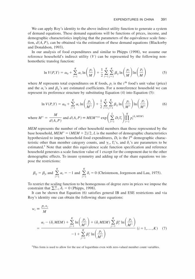
We can apply Roy’s identity to the above indirect utility function to generate a systemof demand equations+ These demand equations will be functions of prices, income, anddemographic characteristics implying that the parameters of the equivalence scale func-tion, d~A,P !, can be obtained via the estimation of these demand equations ~Blackorbyand Donaldson, 1993!+

In our analysis of food expenditures and similar to Phipps ~1998!, we assume ourreference household’s indirect utility ~V ! can be represented by the following non-homothetic translog function:

ln V~P,Y ! � a0 �(i�1

K

ai ln� pi

M��

1

2 (i�1

K

(j�1

K

bij ln� pi

M� ln� pj

M� ~5!

where M represents total expenditures on K foods, pi is the i th food’s unit value ~price!and the ai ’s and bij ’s are estimated coefficients+ For a nonreference household we canrepresent its preference structure by substituting Equation ~4! into Equation ~5!:

ln V~P,Y ! � a0 �(i�1

K

ai ln� pi

M *��1

2 (i�1

K

(j�1

K

bij ln� pi

M *� ln� pj

M *� ~6!

where M * �M

d~A,P !and d~A,P ! [MEM *gs exp�(

l�1

L

Dl Gl�)i�1

K

pi~di MEM !

MEM represents the number of other household members than those represented by thebase household,MEM *� ~MEM � 2!02, L is the number of demographic characteristicshypothesized to impact household food expenditures, Dl is the lth demographic charac-teristic other than member category counts, and gs , Gl ’s, and di ’s are parameters to beestimated+3 Note that under this equivalence scale function specification and referencehousehold generates a scale function value of 1 except for the component due to the otherdemographic effects+ To insure symmetry and adding up of the share equations we im-pose the restrictions:

bij � bji and (i�1

K

ai � �1 and (i�1

K

di � 0 ~Christenson, Jorgenson and Lau, 1975!+

To restrict the scaling function to be homogenous of degree zero in prices we impose theconstraint that ( i�1

K di � 0 ~Phipps, 1998!+It can be shown that Equation ~6! satisfies general IB and ESE restrictions and via

Roy’s identity one can obtain the following share equations:

wi [pi xi

M

�

ai � ~di MEM !�(j�1

K

ln� pj

M *�� ~di MEM ! (j�1

K

bj* ln� pj

M *��1 �(

j�1

K

bj* ln� pj

M *�~i � 1, + + + ,K ! ~7!

3This form is used to allow for the use of logarithms even with zero-valued member count variables+


where bj* �( i�1

K bji Phipps, 1998!+ Given the above share equations, a stochastic errorterm ~ei ! can be added to each share equation where: e; N~0,S! and S is the ~K � K!error term covariance matrix+

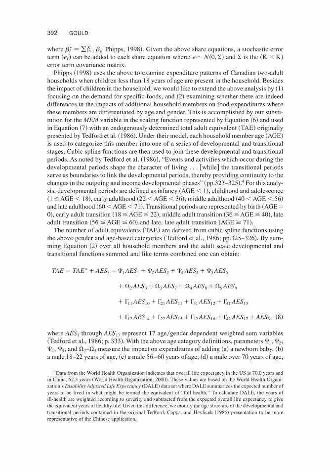
Phipps ~1998! uses the above to examine expenditure patterns of Canadian two-adulthouseholds when children less than 18 years of age are present in the household+ Besidesthe impact of children in the household, we would like to extend the above analysis by ~1!focusing on the demand for specific foods, and ~2! examining whether there are indeeddifferences in the impacts of additional household members on food expenditures wherethese members are differentiated by age and gender+ This is accomplished by our substi-tution for the MEM variable in the scaling function represented by Equation ~6! and usedin Equation ~7! with an endogenously determined total adult equivalent ~TAE! originallypresented by Tedford et al+ ~1986!+Under their model, each household member age ~AGE!is used to categorize this member into one of a series of developmental and transitionalstages+ Cubic spline functions are then used to join these developmental and transitionalperiods+As noted by Tedford et al+ ~1986!, “Events and activities which occur during thedevelopmental periods shape the character of living + + + @while# the transitional periodsserve as boundaries to link the developmental periods, thereby providing continuity to thechanges in the outgoing and income developmental phases” ~pp+323–325!+4 For this analy-sis, developmental periods are defined as infancy ~AGE, 1!, childhood and adolescence~1 � AGE, 18!, early adulthood ~22,AGE, 36!,middle adulthood ~40,AGE, 56!and late adulthood ~60,AGE, 71!+Transitional periods are represented by birth ~AGE �0!, early adult transition ~18 � AGE � 22!,middle adult transition ~36 � AGE � 40!, lateadult transition ~56 � AGE � 60! and late, late adult transition ~AGE � 71!+

The number of adult equivalents ~TAE! are derived from cubic spline functions usingthe above gender and age-based categories ~Tedford et al+, 1986; pp+325–326!+ By sum-ming Equation ~2! over all household members and the adult scale developmental andtransitional functions summed and like terms combined one can obtain:

TAE � TAE * � AES3 �C1 AES1 �C2 AES2 �C4 AES4 �C5 AES5

� V2 AES6 �V3 AES7 �V4 AES8 �V5 AES9

� G11 AES10 � G21 AES11 � G31 AES12 � G41 AES13

� G12 AES14 � G22 AES15 � G32 AES16 � G42 AES17 � AES3 ~8!

where AES1 through AES17 represent 17 age0gender dependent weighted sum variables~Tedford et al+, 1986; p+ 333!+With the above age category definitions, parametersC1,C2 ,C4 , C5 , and V2–V5 measure the impact on expenditures of adding ~a! a newborn baby, ~b!a male 18–22 years of age, ~c! a male 56– 60 years of age, ~d! a male over 70 years of age,

4Data from the World Health Organization indicates that overall life expectancy in the US is 70+0 years andin China, 62+3 years ~World Health Organization, 2000!+ These values are based on the World Health Organi-zation’s Disability Adjusted Life Expectancy ~DALE! data set where DALE summarizes the expected number ofyears to be lived in what might be termed the equivalent of “full health+” To calculate DALE, the years ofill-health are weighted according to severity and subtracted from the expected overall life expectancy to givethe equivalent years of healthy life+ Given this difference, we modify the age structure of the developmental andtransitional periods contained in the original Tedford, Capps, and Havlicek ~1986! presentation to be morerepresentative of the Chinese application+

392 GOULD

~e! a female 18–22 years of age, ~f ! a female 36– 40 years of age, ~g! a female 56– 60years of age, and ~h! a female greater than 70 years of age, respectively+ These parametersare defined relative to the base household member ~and type! which, in the present analy-sis, is assumed to be a single male household member between the ages of 36 and 40~e+g+, C3 � 1!+ The parameters G11–G41 and G12–G42 correspond to the cubic functions formale and female developmental periods, respectively ~p+ 327!+

In their original formulation, Tedford et al+ ~1986! analyze the impact of households ofalternative household compositions on weekly total food expenditures using USDA’s 1977Nationwide Food Consumption Survey+ The authors included an estimate of the total num-ber of adult equivalents in the household and the square of this number as explanatoryvariables to account for the possible existence of economies of size in food purchases+ Inthe present analysis we exclude food purchased and consumed away from home ~FAFH!given the unique determinants that impact such purchases and the inability to define the“price” of FAFH+ Thus, the results to follow should be interpreted in terms of the impactson expenditures on food purchased for at-home consumption+

Given Equation ~8! the scaling function used in the above share equations is:

d~A,P ! [ ~TAE ** !gs exp�(l�1

L

Dl Gl�)i�1

K

pi~di TAE * ! ~9!

where TAE ** is calculated as ~TAE * � 2!02 so that we can take the logarithm ofEquation ~9!+

In their analysis of U+S+ total ~away and at-home! food expenditures, Tedford et al+~1986! obtained estimates of the TAE parameters using a single nonlinear regression modelwhere the dependent variable is total food expenditures and explanatory variables includea set of exogenous variables along with the endogenously determined TAE+ We adopt asimilar procedure here in the sense that we augment the above share equation system inEquation ~7! with the nonlinear regression equation:

M � p0 �p1TAE �p2TAE 2 �pI ln~TOTINC!�pD D * ~10!

where M is total household expenditures for food-at-home, the p’s are coefficients to beestimated, TAE is defined in Equation ~8!, TOTINC is total annual household income, andD* is a vector of other exogenous variables representing refrigerator ownership, degreeof urbanization, and labor force participation by adult household members+ We chose alinear specification with respect to the; estimated p’s given that even under this specifi-cation, Equation ~10! is nonlinear with respect to parameters because of the endog-enously determined TAE variable+ Similar to Tedford et al+ ~1986! we include TAE 2 as anexplanatory variable in the expenditure function to capture possible economies of scale infood-at-home purchases+

In summary, the final econometric model specification consists of the system of shareequations represented by Equation ~7! where the shares are based on at-home food ex-penditures on nine food categories and an auxiliary at-home food expenditure functionrepresented by Equation ~10!+ Because at-home food expenditures is an explanatory vari-able in Equation ~7! and the dependent variable in Equation ~10!, a full-information max-imum likelihood procedure is used to obtain parameter estimates+


3. DATA USED IN THE ANALYSIS

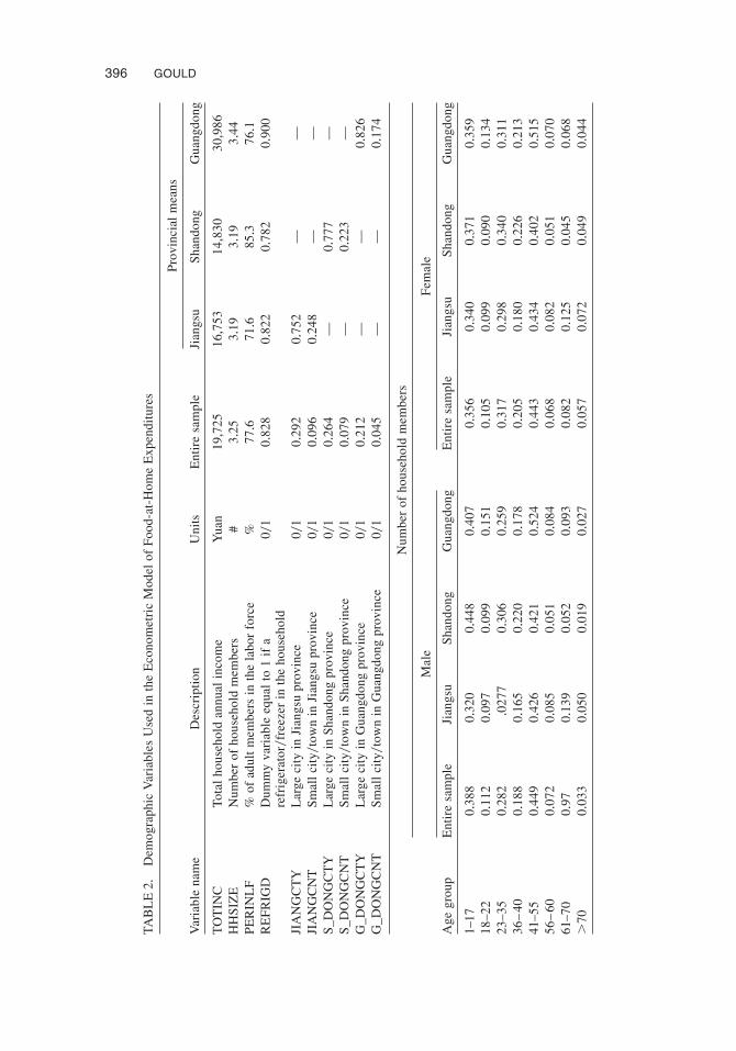
The data used in this analysis was obtained from an annual survey conducted by the StateStatistical Bureau ~SSB! of the People’s Republic of China for 1995–1997+5 This agencyhas had a relatively long history of collecting such data and has separated its data collec-tion efforts into rural and urban components+ For this analysis we use the results of theurban survey for Jiangsu, Shandong, and Guangdong provinces+ In addition to purchasequantity and value information, data as to each household member’s age, gender, educa-tional attainment, household income, and labor force participation characteristics are alsoincluded in this data set+

The unique aspect of this expenditure survey is that households are required to keepdetailed records concerning household expenditures and income over the survey year+The 365-day diary is then summarized by county statistical offices and aggregate resultsfor each expenditure item and household reported to SSB+ This is in contrast to otherhousehold expenditure surveys where diaries encompassing 1–2 weeks which usually meansthat censoring of food expenditures is a significant econometric problem+

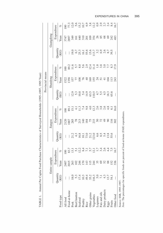
Table 1 provides an overview of the purchase characteristics for a disaggregated list offoods for surveyed households used in this analysis+ There are some differences in pur-chase patterns across provinces+As will be noted in Table 2, Guangdong province is rel-atively affluent+ Higher provincial incomes is part of the explanation for more than twicethe level of per capita food expenditures observed than in Shandong province+ Away-from-home expenditures account for more of total food expenditures, 23% in Guangdongvs+ 11% in the other two provinces+ In terms of the distribution of food-at-home expen-ditures there are also some provincial differences+ For example, in Guangdong, 15% ofat-home per capita expenditure is for seafood+ This compares to 8% for Shandong+ Slightlymore than 12% of Shandong at-home expenditures ~FAH! is for Grains0Flour ~includingbread!+ This is in contrast to 4% observed for households in Guangdong province+

For our analysis we adopt the following commodity group definitions: pork, beef0mutton, poultry, sea food, total grains, fruits, vegetables, dairy products and eggs, andother foods+ We use these categories to avoid problems of censoring of commodity de-mands such as those outlined in Gao et al+ ~1996!+Again, the expenditures represented bythe above categories do not include any food purchases that are purchased and consumedout of the home ~e+g+, restaurant expenditures!+

Table 2 provides an overview of exogenous household characteristics+ Besides dra-matic differences in income as noted above, we see that there are differences in the per-cent of adult household members in the labor force with an average 85+3% of adult membersin Shandong vs+ 71+6% in Jiangsu province+ There is also a difference in the percent of thesampled households where there is refrigerated storage, 78+2% of households in Shan-dong vs+ 90+0% in Guangdong province+

4. ECONOMETRIC RESULTS

To estimate the econometric model we eliminated observations due to missing data, thepresence of extremely large unit values ~prices!, and households that fed nonresidents out

5For a discussion of the availability of food consumption data for China, refer to Chern ~1994!+ All expen-ditures have been deflated to $1995 yuan using consumer price inflation figures available from U+S+ Depart-ment of State ~2000!+

394 GOULD

TAB

LE

1+A

nnua

lP

erC

apit

aF

ood

Pur

chas

eC

hara

cter

isti

csof

Sur

veye

dH

ouse

hold

s~1

995–

1997,1

995

Yua

n!

Pro

vinc

ial

mea

ns

Ent

ire

sam

ple

Jian

gsu

Sha

ndon

gG

uang

dong

Exp

endi

ture

Exp

endi

ture

Exp

endi

ture

Exp

endi

ture

Foo

dty

peQ

uant

ity

~KG!

Yua

n%

Qua

ntit

y~K

G!

Yua

n%

Qua

ntit

y~K

G!

Yua

n%

Qua

ntit

y~K

G!

Yua

n%

All

food

—24

0710

0—

2120

100

—15

2210

0—

3747

100

Foo

d-at

-hom

e—

2015

83+7

—18

8789+1

—13

5889+2

—28

9777+3

Por

k18+0

263

13+1

21+2

285

15+1

12+9

157

11+6

19+0

349

12+0

Bee

f0m

utto

n5+

310

25+

14+

378

4+1

5+3

775+

76+

716

15+

6S

eafo

od17+4

246

12+2

16+8

213

11+3

10+8

108

8+0

25+3

440

15+2

Pou

ltry

10+3

170

8+4

10+1

140

7+4

5+4

765+

616+1

310

10+7

Ric

e49+4

143

7+1

73+0

184

9+8

14+9

402+

955+6

201

6+9

Oth

ergr

ains

35+2

115

5+7

21+2

754+

063+5

169

12+4

15+6

109

3+8

Veg

etab

les

116+

324

412+1

123+

023

312+3

110+

515

511+4

113+

735

412+2

Leg

umes

5+0

351+

76+

650

2+6

4+7

241+

83+

226

0+9

Fat

san

doi

ls7+

169

3+4

8+5

723+

85+

551

3+8

6+9

852+

9D

airy

prod

ucts

4+3

522+

65+

449

2+6

4+5

413+

02+

668

2+3

Egg

s13+7

884+

413+8

904+

818+3

104

7+7

8+7

692+

4F

ruit

s54+1

152

7+5

55+6

116

6+1

65+6

113

8+3

39+5

242

8+4

Oth

erfo

od—

336

16+7

—30

216+0

—24

317+9

—48

316+7

Sou

rce:

SS

B,1

995–

1997+

Not

e:T

hepe

rcen

tage

sfo

rsp

ecif

icfo

ods

are

perc

ent

offo

od-a

t-ho

me~F

AH!

expe

ndit

ures+


TAB

LE

2+D

emog

raph

icV

aria

bles

Use

din

the

Eco

nom

etri

cM

odel

ofF

ood-

at-H

ome

Exp

endi

ture

s

Pro

vinc

ial

mea

ns

Var

iabl

ena

me

Des

crip

tion

Uni

tsE

ntir

esa

mpl

eJi

angs

uS

hand

ong

Gua

ngdo

ng

TO

TIN

CTo

tal

hous

ehol

dan

nual

inco

me

Yua

n19,7

2516,7

5314,8

3030,9

86H

HS

IZE

Num

ber

ofho

useh

old

mem

bers

#3+

253+

193+

193+

44P

ER

INL

F%

ofad

ult

mem

bers

inth

ela

bor

forc

e%

77+6

71+6

85+3

76+1

RE

FR

IGD

Dum

my

vari

able

equa

lto

1if

are

frig

erat

or0f

reez

erin

the

hous

ehol

d00

10+

828

0+82

20+

782

0+90

0

JIA

NG

CT

YL

arge

city

inJi

angs

upr

ovin

ce00

10+

292

0+75

2—

—JI

AN

GC

NT

Sm

all

city0t

own

inJi

angs

upr

ovin

ce00

10+

096

0+24

8—

—S

_DO

NG

CT

YL

arge

city

inS

hand

ong

prov

ince

001

0+26

4—

0+77

7—

S_D

ON

GC

NT

Sm

all

city0t

own

inS

hand

ong

prov

ince

001

0+07

9—

0+22

3—

G_D

ON

GC

TY

Lar

geci

tyin

Gua

ngdo

ngpr

ovin

ce00

10+

212

——

0+82

6G

_DO

NG

CN

TS

mal

lci

ty0t

own

inG

uang

dong

prov

ince

001

0+04

5—

—0+

174

Num

ber

ofho

useh

old

mem

bers

Mal

eF

emal

e

Age

grou

pE

ntir

esa

mpl

eJi

angs

uS

hand

ong

Gua

ngdo

ngE

ntir

esa

mpl

eJi

angs

uS

hand

ong

Gua

ngdo

ng

1–17

0+38

80+

320

0+44

80+

407

0+35

60+

340

0+37

10+

359

18–2

20+

112

0+09

70+

099

0+15

10+

105

0+09

90+

090

0+13

423

–35

0+28

2+0

277

0+30

60+

259

0+31

70+

298

0+34

00+

311

36–

400+

188

0+16

50+

220

0+17

80+

205

0+18

00+

226

0+21

341

–55

0+44

90+

426

0+42

10+

524

0+44

30+

434

0+40

20+

515

56–

600+

072

0+08

50+

051

0+08

40+

068

0+08

20+

051

0+07

061

–70

0+97

0+13

90+

052

0+09

30+

082

0+12

50+

045

0+06

8.

700+

033

0+05

00+

019

0+02

70+

057

0+07

20+

049

0+04

4

396 GOULD

of home food supplies+ Our final sample size consisted of 5273 households+ We use aFIML estimator with the GAUSSX software system to estimate the 10-equation systemrepresented by Equations ~7! and ~10! where the TAE and scaling functions are defined inEquations ~8! and ~9!, respectively, and the TAE variable is used in place of MEM inEquation ~7!+ Tables 3 and 4 provide estimated coefficients for various components of theeconometric model+ Table 5 provides the likelihood function value for the base modelalong with individual R2 values for the share and total food expenditure equations+

4.1. Adult Equivalent Parameter Estimates

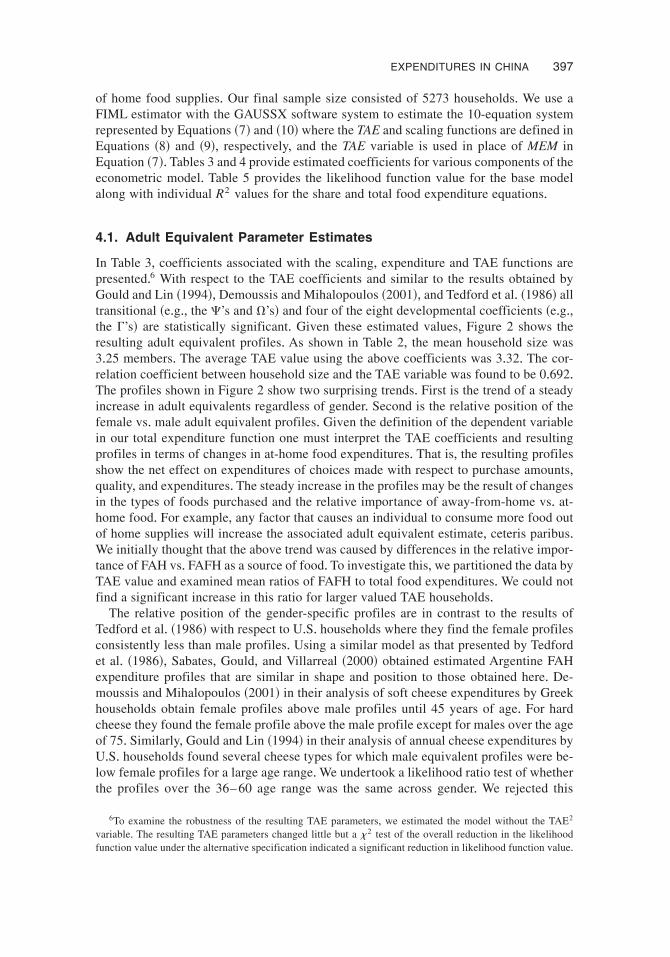
In Table 3, coefficients associated with the scaling, expenditure and TAE functions arepresented+6 With respect to the TAE coefficients and similar to the results obtained byGould and Lin ~1994!, Demoussis and Mihalopoulos ~2001!, and Tedford et al+ ~1986! alltransitional ~e+g+, the C’s and V’s! and four of the eight developmental coefficients ~e+g+,the G’s! are statistically significant+ Given these estimated values, Figure 2 shows theresulting adult equivalent profiles+ As shown in Table 2, the mean household size was3+25 members+ The average TAE value using the above coefficients was 3+32+ The cor-relation coefficient between household size and the TAE variable was found to be 0+692+The profiles shown in Figure 2 show two surprising trends+ First is the trend of a steadyincrease in adult equivalents regardless of gender+ Second is the relative position of thefemale vs+ male adult equivalent profiles+ Given the definition of the dependent variablein our total expenditure function one must interpret the TAE coefficients and resultingprofiles in terms of changes in at-home food expenditures+ That is, the resulting profilesshow the net effect on expenditures of choices made with respect to purchase amounts,quality, and expenditures+ The steady increase in the profiles may be the result of changesin the types of foods purchased and the relative importance of away-from-home vs+ at-home food+ For example, any factor that causes an individual to consume more food outof home supplies will increase the associated adult equivalent estimate, ceteris paribus+We initially thought that the above trend was caused by differences in the relative impor-tance of FAH vs+ FAFH as a source of food+ To investigate this, we partitioned the data byTAE value and examined mean ratios of FAFH to total food expenditures+We could notfind a significant increase in this ratio for larger valued TAE households+

The relative position of the gender-specific profiles are in contrast to the results ofTedford et al+ ~1986! with respect to U+S+ households where they find the female profilesconsistently less than male profiles+ Using a similar model as that presented by Tedfordet al+ ~1986!, Sabates, Gould, and Villarreal ~2000! obtained estimated Argentine FAHexpenditure profiles that are similar in shape and position to those obtained here+ De-moussis and Mihalopoulos ~2001! in their analysis of soft cheese expenditures by Greekhouseholds obtain female profiles above male profiles until 45 years of age+ For hardcheese they found the female profile above the male profile except for males over the ageof 75+ Similarly, Gould and Lin ~1994! in their analysis of annual cheese expenditures byU+S+ households found several cheese types for which male equivalent profiles were be-low female profiles for a large age range+We undertook a likelihood ratio test of whetherthe profiles over the 36– 60 age range was the same across gender+ We rejected this

6To examine the robustness of the resulting TAE parameters, we estimated the model without the TAE2

variable+ The resulting TAE parameters changed little but a x2 test of the overall reduction in the likelihoodfunction value under the alternative specification indicated a significant reduction in likelihood function value+


TAB

LE

3+E

stim

ated

Sca

ling,E

xpen

ditu

re,a

ndTA

EF

unct

ion

Coe

ffic

ient

s

Sca

ling

Fun

ctio

n@E

q+~9!#

Exp

endi

ture

Fun

ctio

n@E

q+~1

0!#

TAE

Fun

ctio

n@E

q+~8!#

Var

iabl

eC

oeff

icie

ntS

EV

aria

ble

Coe

ffic

ient

SE

Var

iabl

eC

oeff

icie

ntS

E

TAE*

0+73

83*

0+19

05In

terc

ept

�0+

5571

*0+

0641

AE

S1

0+49

52*

0+13

18R

EF

RIG

D0+

0879

*0+

0218

TAE

0+05

57*

0+02

42A

ES

20+

7240

*0+

0943

LN~T

OT

INC!

0+32

81*

0+01

97TA

E2

0+01

22*

0+00

39A

ES

41+

3351

*0+

1416

PE

RIN

LF

0+00

640+

0289

RE

FR

IGD

0+02

77*

0+01

35A

ES

51+

5698

*0+

2013

G_D

ON

GC

TY

1+72

15*

0+04

10P

ER

INL

F0+

6072

*0+

0147

AE

S6

1+54

92*

0+07

80G

_DO

NG

CN

T1+

5273

*0+

0496

LN~T

OT

INC!

0+63

37*

0+01

98A

ES

71+

3415

*0+

2304

JIA

NG

CT

Y0+

6486

*0+

0230

G_D

ON

GC

TY

0+16

33*

0+01

39A

ES

81+

9627

*0+

2624

JIA

NG

CN

T0+

2576

*0+

0286

G_D

ON

GC

NT

�0+

0097

0+01

99A

ES

91+

1128

*0+

1518

S_D

ON

GC

NT

�0+

3748

*0+

0342

JIA

NG

CT

Y�

0+15

35*

0+02

84A

ES

10�

0+16

05*

0+05

46A

ES

_PO

RK

0+00

55*

0+00

16JI

AN

GC

NT

0+03

200+

0188

AE

S11

�0+

0189

0+02

75A

ES

_RE

DM

T�

0+00

22*

0+00

06S

_DO

NG

CN

T0+

1946

*0+

0104

AE

S12

0+02

040+

0470

AE

S_P

OU

LT�

0+00

52*

0+00

17E

last

icit

ies

AE

S13

0+17

46*

0+05

13A

ES

_SE

AF

D�

0+00

090+

0018

INC

OM

E0+

1956

0+01

05A

ES

14�

0+17

69*

0+05

14A

ES

_GR

AIN

0+01

35*

0+00

32TA

E0+

4556

0+02

03A

ES

15�

0+09

96*

0+03

20A

ES

_VE

G0+

0024

*0+

0007

AE

S16

�0+

0823

0+04

74A

ES

_FR

UIT

�0+

0091

*0+

0012

AE

S17

0+01

210+

0484

AE

S_D

PE

GG

�0+

0007

0+00

15A

ES

_OT

HE

R�

0+00

320+

0024

Not

e:T

heA

ES

_Jte

rms

corr

espo

ndto

thed’

sap

pear

ing

inth

esc

alin

gfu

ncti

on+

The

*sy

mbo

lin

the

coef

fici

ent

colu

mn

indi

cate

ssi

gnif

ican

ceat

the+0

1le

vel+

398 GOULD

hypothesis at the 0+01 level of significance+Again, these results do not imply that middle-aged females eat more food than middle-aged males but instead implies that at-homefood expenditures are greater+ These relatively higher expenditures may be the result of anumber of unique food purchase decisions such as the purchase of foods with improvedquality ~and reflected in higher per unit prices! and reduced use of away-from home foodsources+7

To quantify whether there are significant differences between male and female adultprofiles, we tested the null hypothesis that they are the same over all age levels+ Therestricted model resulting from the hypothesis of equality of profiles across gender rep-resents a nested version of the unrestricted specification+ As such, we use a likelihoodratio test procedure to examine the null hypothesis+ In Table 5 we show the results of thistest+ The x8 d+f+

2 test statistic with a value of 38+8 is significant at the 99% level and impliesthat the male and female profiles shown in Figure 2 are indeed statistically different+ Incomparison, Sabates, Gould, and Villarreal ~2000! use the Tedford et al+ ~1986! approachto estimate total food TAE profile for urban households in Argentina, Brazil, and Mexico+In their analysis they rejected the null hypothesis that the female and male profiles wereequivalent under the Argentine and Mexican analyses and could not reject this hypothesisfor Brazil+With the TAE-based model having a significantly greater likelihood functionvalue than the member count specification, we can infer that the former model providesa better representation of the structure of food demand+

7The SSB data used here did not allow us to identify FAFH expenditures for specific household members+Assuch, we could not directly examine the role of FAFH for households with middle-aged females vs+ males+Given the extended household structure there were a limited number of households with just one middle-agedadult which again limited our ability to test this hypothesis+

Figure 2Food-at-home adult equivalent values+


To examine the importance of using the TAE function in place of the traditional mea-sure of household size, we conduct a test of the overall improvement of the above econo-metric model by its use vs+ that of a simple count of household members+ Since the testingof the adult equivalent vs+ household size implies the assumption that each member has aweight of 1+0, this is essentially a test of the original Phipps ~1998! model structure+ A

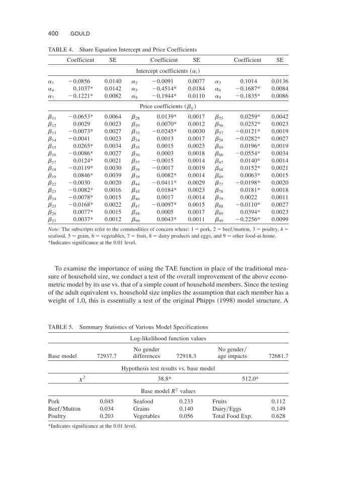
TABLE 4+ Share Equation Intercept and Price Coefficients

Coefficient SE Coefficient SE Coefficient SE

Intercept coefficients ~ai !

a1 �0+0856 0+0140 a2 �0+0091 0+0077 a3 0+1014 0+0136a4 0+1037* 0+0142 a5 �0+4514* 0+0184 a6 �0+1687* 0+0084a7 �0+1221* 0+0082 a8 �0+1944* 0+0110 a9 �0+1835* 0+0086

Price coefficients ~bij !

b11 �0+0653* 0+0064 b28 0+0139* 0+0017 b55 0+0259* 0+0042b12 0+0029 0+0023 b29 0+0070* 0+0012 b56 0+0252* 0+0023b13 �0+0073* 0+0027 b33 �0+0245* 0+0030 b57 �0+0121* 0+0019b14 �0+0041 0+0023 b34 0+0013 0+0017 b58 �0+0282* 0+0027b15 0+0265* 0+0034 b35 0+0015 0+0023 b59 0+0196* 0+0019b16 �0+0086* 0+0027 b36 0+0003 0+0018 b66 �0+0554* 0+0034b17 0+0124* 0+0021 b37 �0+0015 0+0014 b67 0+0140* 0+0014b18 �0+0119* 0+0030 b38 �0+0017 0+0019 b68 0+0152* 0+0021b19 0+0846* 0+0039 b39 0+0082* 0+0014 b69 0+0063* 0+0015b22 �0+0030 0+0020 b44 �0+0411* 0+0029 b77 �0+0198* 0+0020b23 �0+0082* 0+0016 b45 0+0184* 0+0023 b78 0+0181* 0+0018b24 �0+0078* 0+0015 b46 0+0017 0+0014 b79 0+0022 0+0011b25 �0+0168* 0+0022 b47 �0+0097* 0+0015 b88 �0+0110* 0+0027b26 0+0077* 0+0015 b48 0+0005 0+0017 b89 0+0394* 0+0023b27 0+0037* 0+0012 b99 0+0043* 0+0011 b99 �0+2256* 0+0099

Note: The subscripts refer to the commodities of concern where: 1 � pork, 2 � beef0mutton, 3 � poultry, 4 �seafood, 5 � grain, 6 � vegetables, 7 � fruit, 8 � dairy products and eggs, and 9 � other food-at-home+*Indicates significance at the 0+01 level+

TABLE 5+ Summary Statistics of Various Model Specifications

Log-likelihood function values

Base model 72937+7No genderdifferences 72918+3

No gender0age impacts 72681+7

Hypothesis test results vs+ base model

x2 38+8* 512+0*

Base model R2 values

Pork 0+045 Seafood 0+233 Fruits 0+112Beef0Mutton 0+034 Grains 0+140 Dairy0Eggs 0+149Poultry 0+203 Vegetables 0+056 Total Food Exp+ 0+628

*Indicates significance at the 0+01 level+

400 GOULD

likelihood ratio test is used to determine if there is a significant improvement in explan-atory power of the model when incorporating the TAE variable+ In Table 5 we see that theresulting x16 d+f+

2 of 512+0 is statistically significant indicating that the inclusion of theendogenously determined TAE variable improves the explanatory power of the model+

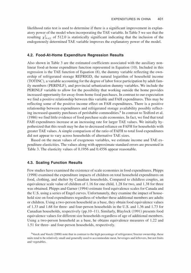
4.2. Food-At-Home Expenditure Regression Results

Also shown in Table 3 are the estimated coefficients associated with the auxiliary non-linear food-at-home expenditure function represented in Equation ~10!+ Included in thisregression is the TAE function of Equation ~8!, the dummy variable reflecting the own-ership of refrigerated storage REFRIGD, the natural logarithm of household income~TOTINC!, a variable accounting for the degree of labor force participation by adult fam-ily members ~PERINLF!, and provincial urbanization dummy variables+We include thePERINLF variable to allow for the possibility that working outside the home providesincreased opportunity for away-from-home food purchases+ In contrast to our expectationwe find a positive relationship between this variable and FAH expenditures+ This may bereflecting some of the positive income effect on FAH expenditures+ There is a positiverelationship between expenditures and refrigerated storage availability possibly reflect-ing increased quantity purchases of perishable commodities+8 In contrast to Tedford et al+~1986! we find little evidence of food purchase scale economies+ In fact, we find that totalFAH expenditures increase at an increasing rate for larger TAE values+ We initially hy-pothesized that this result may be due to decreased reliance on FAFH for households withgreater TAE values+A simple comparison of the ratio of FAFH to total food expendituresdid not appear to vary across households of alternative TAE sizes+

Based on the mean values of exogenous variables, we estimate income and TAE ex-penditure elasticities+ The values along with approximate standard errors are presented inTable 3+ The elasticity values of 0+1956 and 0+4556 appear reasonable+

4.3. Scaling Function Results

Few studies have examined the existence of scale economies in food expenditures+ Phipps~1998! examined the expenditure impacts of children on total household expenditures onfood, clothing, and shelter by Canadian households+ Compared to childless couples, anequivalence scale value of children of 1+16 for one child, 1+28 for two, and 1+38 for threewas obtained+ Phipps and Garner ~1994! estimate food equivalence scales for Canada andthe U+S+ using a series of Engel curves+ Unfortunately, they examine the impact of house-hold size on food expenditures regardless of whether these additional members are adultsor children+ Using a two-person household as a base, they obtain food equivalence valuesof 1+33 and 1+68 for three- and four-person households in the U+S+ and 1+36 and 1+73 forCanadian households, respectively ~pp+10–11!+ Similarly, Blaylock ~1991! presents foodequivalence values for different size households regardless of age of additional members+Using a two-person household as a base, he obtains equivalence measures of 1+22 and1+51 for three- and four-person households, respectively+

8Veeck and Veeck ~2000! note that in contrast to the high percentage of refrigerator0freezer ownership, theseunits tend to be relatively small and generally used to accommodate meat, beverages and leftovers, but not fruitsand vegetables+


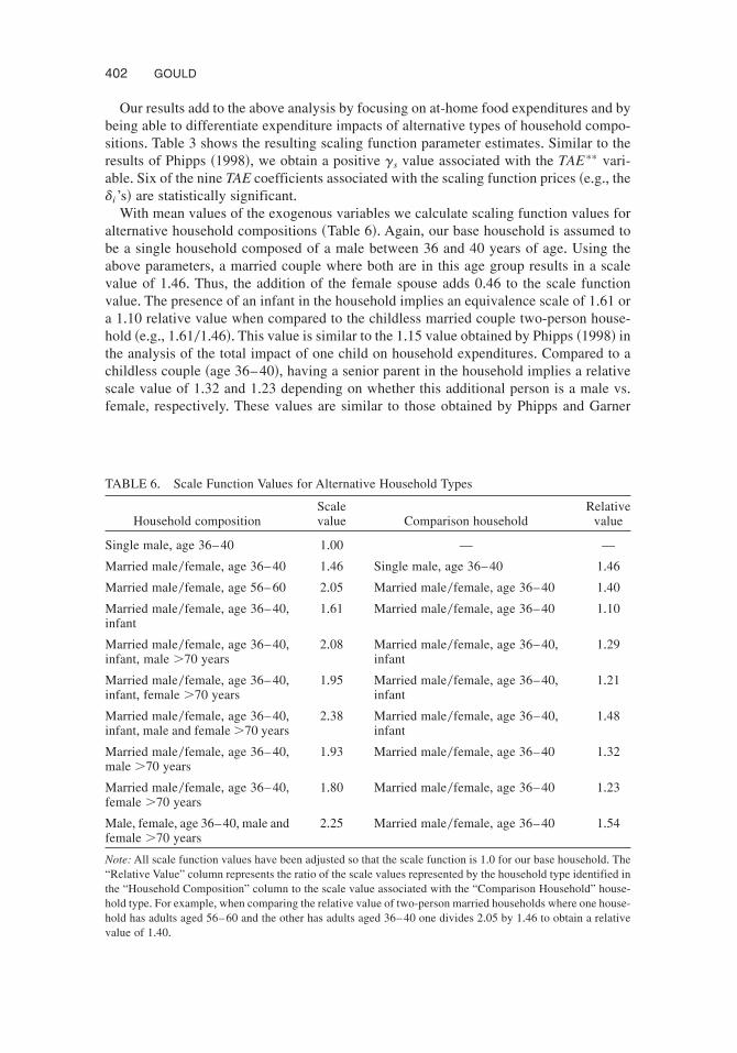
Our results add to the above analysis by focusing on at-home food expenditures and bybeing able to differentiate expenditure impacts of alternative types of household compo-sitions+ Table 3 shows the resulting scaling function parameter estimates+ Similar to theresults of Phipps ~1998!, we obtain a positive gs value associated with the TAE ** vari-able+ Six of the nine TAE coefficients associated with the scaling function prices ~e+g+, thedi ’s! are statistically significant+

With mean values of the exogenous variables we calculate scaling function values foralternative household compositions ~Table 6!+ Again, our base household is assumed tobe a single household composed of a male between 36 and 40 years of age+ Using theabove parameters, a married couple where both are in this age group results in a scalevalue of 1+46+ Thus, the addition of the female spouse adds 0+46 to the scale functionvalue+ The presence of an infant in the household implies an equivalence scale of 1+61 ora 1+10 relative value when compared to the childless married couple two-person house-hold ~e+g+, 1+6101+46!+ This value is similar to the 1+15 value obtained by Phipps ~1998! inthe analysis of the total impact of one child on household expenditures+ Compared to achildless couple ~age 36– 40!, having a senior parent in the household implies a relativescale value of 1+32 and 1+23 depending on whether this additional person is a male vs+female, respectively+ These values are similar to those obtained by Phipps and Garner

TABLE 6+ Scale Function Values for Alternative Household Types

Household compositionScalevalue Comparison household

Relativevalue

Single male, age 36– 40 1+00 — —

Married male0female, age 36– 40 1+46 Single male, age 36– 40 1+46

Married male0female, age 56– 60 2+05 Married male0female, age 36– 40 1+40

Married male0female, age 36– 40,infant

1+61 Married male0female, age 36– 40 1+10

Married male0female, age 36– 40,infant, male .70 years

2+08 Married male0female, age 36– 40,infant

1+29

Married male0female, age 36– 40,infant, female .70 years


1+21

Married male0female, age 36– 40,infant, male and female.70 years


1+48

Married male0female, age 36– 40,male .70 years


Married male0female, age 36– 40,female .70 years


Male, female, age 36–40,male andfemale .70 years


Note: All scale function values have been adjusted so that the scale function is 1+0 for our base household+ The“Relative Value” column represents the ratio of the scale values represented by the household type identified inthe “Household Composition” column to the scale value associated with the “Comparison Household” house-hold type+ For example, when comparing the relative value of two-person married households where one house-hold has adults aged 56– 60 and the other has adults aged 36– 40 one divides 2+05 by 1+46 to obtain a relativevalue of 1+40+

402 GOULD

~1994! and Blaylock ~1991!+ The 1+54 relative value obtained for a household with twoseniors in a childless couple household ~age 36– 40! is also similar to the values obtainedin these previous analyses+

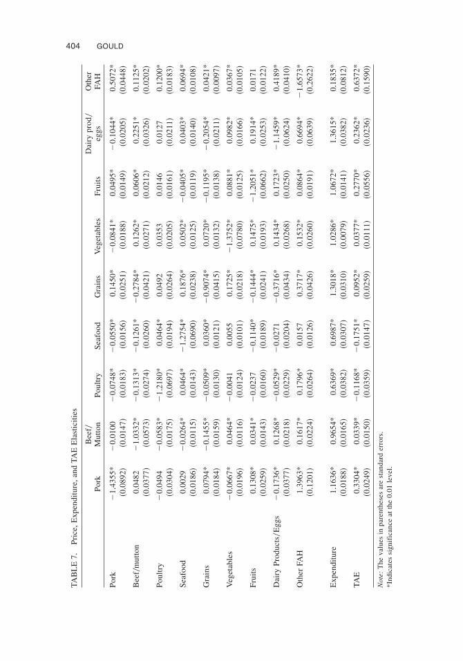
4.4. Estimated Price and Expenditure Demand Elasticities

Given the translog share equations in Equation ~7! we estimate own and cross-price elas-ticities of the demand for the nine foods delineated in our analysis+ In addition to theparameter estimates displayed in Table 3, the price coefficients in Table 4 are required toevaluate these elasticities+ From the above we see that seven of the nine share equationintercept terms, are statistically significant, and of reasonable magnitude+9 Except for beef0mutton, all of the own-price coefficients ~bii ’s! are statistically significant+ More than75% of the 45 price coefficients ~bif ’s! were found to be statistically significant+

Given the coefficients displayed in Tables 3 and 4, we estimate uncompensated ownand cross price-elasticities evaluated at the mean values of the exogenous variables alongwith their standard errors are displayed in Table 7+More than 80% of the estimated elas-ticities were found to be significantly different from 0+ All of own price elasticities arenegative and elastic with the exception of the beef0mutton and grain commodities withthe grain own-price elasticity being significantly less than �1+0+10 The cross-price elas-ticities are of reasonable sign with a large number of estimated substitute relationships+

Our price elasticity results can be compared with previous demand system approachesto the analysis of Chinese food demand+ Gao et al+ ~1996! estimate a nine equation fooddemand system which closely parallels the definitions of the food groups used here+ Theelasticities obtained in their analysis tended to be less elastic+ None of their own-priceelasticities were found to less than �1+0 + For some own-price elasticities, however, ourresults compare quite favorably with theirs+ For example, our grain own-price elastictityof �0+907 is very close to their value of �0+988+ Han and Wahl ~1998! in their analysisof rural 1993 Chinese food demand obtained a grain elasticity of �0+784+ In contrast, weobtain a vegetable own-price elasticity of �1+375 compared to Gao et al+ ~1996! value of�0+834 and own-price elasticities of between �0+863 and �0+182 for a variety of veg-etable types obtained by Han and Wahl ~1998!+

Estimated expenditure elasticities are displayed in the last row of Table 7+ All of theelasticities are positive except beef0mutton, pork, and seafood are statistically greaterthan 1+0 implying that these three commodities may be considered necessities+ Peterson,Jin, and Ito ~1991! note, in many Asian countries, rice appears to have become an inferiorgood+ That is, as incomes have increased in this area there has been a substitution awayfrom rice to other food products+ elasticity of �0+248 for 1995 under a low growth sce-

9The omitted parameters are obtained from adding up and homogeneity conditions+ For these parameters andfor the elasticities discussed below approximate standard errors are derived from the estimated parameter variance-covariance matrix:

Var~d~Q!! � C(Q

C ' where C �]d~Q!

]Q',

Q is the vector of estimated coefficients d~Q! is the estimated equivalence scale and (Q is the coefficientcovariance matrix+

10When interpreting the grain elasticities it should be noted that both raw and processed grain-based prod-ucts such as breads are incorporated in the aggregate grain commodity+


TAB

LE

7+P

rice,E

xpen

ditu

re,a

ndTA

EE

last

icit

ies

Por

kB

eef0

Mut

ton

Pou

ltry

Sea

food

Gra

ins

Veg

etab

les

Fru

its

Dai

rypr

od0

eggs

Oth

erFA

H

Por

k�

1+43

55*

�0+

0100

�0+

0748

*�

0+05

50*

0+14

50*

�0+

0841

*0+

0495

*�

0+10

44*

0+50

72*

~0+0

892!

~0+0

147!

~0+0

183!

~0+0

156!

~0+0

251!

~0+0

188!

~0+0

149!

~0+0

205!

~0+0

448!

Bee

f0m

utto

n0+

0482

�1+

0332

*�

0+13

13*

�0+

1261

*�

0+27

84*

0+12

62*

0+06

06*

0+22

51*

0+11

25*

~0+0

377!

~0+0

573!

~0+0

274!

~0+0

260!

~0+0

421!

~0+0

271!

~0+0

212!

~0+0

326!

~0+0

202!

Pou

ltry

�0+

0494

�0+

0583

*�

1+21

80*

0+04

64*

0+04

920+

0353

0+01

460+

0127

0+12

00*

~0+0

304!

~0+0

175!

~0+0

697!

~0+0

194!

~0+0

264!

~0+0

205!

~0+0

161!

~0+0

211!

~0+0

183!

Sea

food

0+00

29�

0+02

64*

0+04

64*

�1+

2754

*0+

1876

*0+

0502

*�

0+04

05*

0+04

03*

0+06

94*

~0+0

186!

~0+0

115!

~0+0

143!

~0+0

690!

~0+0

238!

~0+0

125!

~0+0

119!

~0+0

140!

~0+0

108!

Gra

ins

0+07

94*

�0+

1455

*�

0+05

09*

0+03

60*

�0+

9074

*0+

0720

*�

0+11

95*

�0+

2054

*0+

0421

*~0+0

184!

~0+0

159!

~0+0

130!

~0+0

121!

~0+0

415!

~0+0

132!

~0+0

138!

~0+0

211!

~0+0

097!

Veg

etab

les

�0+

0667

*0+

0464

*�

0+00

410+

0055

0+17

25*

�1+

3752

*0+

0881

*0+

0982

*0+

0367

*~0+0

196!

~0+0

116!

~0+0

124!

~0+0

101!

~0+0

218!

~0+0

780!

~0+0

125!

~0+0

166!

~0+0

105!

Fru

its

0+13

08*

0+03

41*

�0+

0237

�0+

1140

*�

0+14

44*

0+14

75*

�1+

2051

*0+

1914

*0+

0171

~0+0

259!

~0+0

143!

~0+0

160!

~0+0

189!

~0+0

241!

~0+0

193!

~0+0

662!

~0+0

253!

~0+0

122!

Dai

ryP

rodu

cts0

Egg

s�

0+17

36*

0+12

68*

�0+

0529

*�

0+02

71�

0+37

16*

0+14

34*

0+17

23*

�1+

1459

*0+

4189

*~0+0

377!

~0+0

218!

~0+0

229!

~0+0

204!

~0+0

434!

~0+0

268!

~0+0

250!

~0+0

624!

~0+0

410!

Oth

erFA

H1+

3963

*0+

1617

*0+

1796

*0+

0157

0+37

17*

0+15

32*

0+08

64*

0+66

94*

�1+

6573

*~0+1

201!

~0+0

224!

~0+0

264!

~0+0

126!

~0+0

426!

~0+0

260!

~0+0

191!

~0+0

639!

~0+2

622!

Exp

endi

ture

1+16

36*

0+96

54*

0+63

69*

0+69

87*

1+30

18*

1+02

86*

1+06

72*

1+36

15*

0+18

35*

~0+0

188!

~0+0

165!

~0+0

382!

~0+0

307!

~0+0

310!

~0+0

079!

~0+0

141!

~0+0

382!

~0+0

812!

TAE

0+33

04*

0+03

39*

�0+

1168

*�

0+17

51*

0+09

52*

0+03

77*

0+27

70*

0+23

62*

0+63

72*

~0+0

249!

~0+0

150!

~0+0

359!

~0+0

147!

~0+0

259!

~0+0

111!

~0+0

556!

~0+0

236!

~0+1

590!

Not

e:T

heva

lues

inpa

rent

hese

sar

est

anda

rder

rors+

*Ind

icat

essi

gnif

ican

ceat

the

0+01

leve

l+

404 GOULD

nario ~Peterson, Jin, & Ito, 1991, p+74!+11 Our cross-sectional results contrast with theabove given that our grains expenditure elasticity ~where our grains category includesrice! is greater than 1+0 +

5. CONCLUSIONS

The results from this analysis show that Chinese food demand is sensitive to price changes+Surprisingly, we find that the own-price elasticity for beef0mutton not to be significantlydifferent from 1+0+ Purchases of pork were found to be the most sensitive to own pricechanges ~except for the “other food” category!+We find that total household FAH expen-ditures are positively related to the number of adult equivalents in the household, income,and on whether the household has refrigerated storage+We also found significant varia-tion in expenditures across regions and subregions+

We find that household composition matters in determining the demand for specificgoods+ This result was obtained via the use of the endogenously determined TAE variableas a stand-alone variable in scaling function ~e+g+, TAE** ! and as a multiplier to eachprice in this scaling function+ For example, from the estimated coefficients we can eval-uate the elasticity impacts of a change in the number of adult equivalents on the demandfor the commodities delineated in our demand system+ The last row of Table 7 showsthese elasticities+Our results indicate that as the number of adult equivalents in the house-hold increases ~and given constant food expenditures! households tend to adjust theirexpenditures such that the demand for poultry and seafood decrease and the demand forother foods increase with the largest increases for other foods, pork, and other food-at-home expenditures+ This is important information to potential food exporters as the struc-ture of the Chinese household changes over time+

ACKNOWLEDGMENTS

The author would like to thank the Babcock Institute for Dairy Research and Develop-ment and the College of Agricultural and Life Sciences at the University of Wisconsin-Madison for providing the financial support for this research+ Any errors or omissionsremain the responsibility of the author+ The comments of two reviewers greatly improvedthe manuscript’s quality and is gratefully acknowledged+

REFERENCES

Blackorby, C+, & Donaldson, D+ ~1993!+ Adult equivalence scales and the economic implementa-tion of interpersonal comparisons of well-being+ Social Choice and Welfare, 10~4!, 335–361+

Blaylock, J+ ~1991!+ The impact of equivalence scales on the analysis of income and food spendingdistributions+Western Journal of Agricultural Economics, 16~1!, 11–20+

11There is considerable debate as to whether rice becomes an inferior good as income increases in Asiancountries+ For an overview refer to Huang, David, and Duff ~1991!, Bouis ~1991! and Ito, Peterson, and Grant~1991!+ This large grain expenditure elasticity is in contrast to previous analyses but not unprecedented+ Forexample, in Han and Wahl ~1998! they obtain an estimated conditional grain expenditure elasticity of 1+092with a range of 1+214 for high-income rural households to 1+067 for medium-income rural households+ Guan~1996! in an analysis of urban China and Chi ~1995! in an analysis of rural China obtain estimated grain ex-penditure elasticities of 0+9110 and 1+1125+ Gao et al+ ~1996! obtained a grain elasticity of 0+5164 which issignificantly less than 1+0+


Blundell, R+,& Lewbel,A+ ~1991!+ The information content of equivalence scales+ Journal of Econo-metrics, 50, 49– 68+

Bouis, H+ ~1991!+ Rice in Asia: Is it becoming a commercial good? Comment+American Journal ofAgricultural Economics, 73~2!, 522–527+

Chern, W+S+ ~1994!+ Consumption and Demand Data in the People’s Republic of China+ In Wahl,T+I+ & O’Rourke, A+D+ ~Eds+!, China as a Market and Competitor+ Proceedings of RegionalCommittee WRCC-101, Reno NV, Nov+ 1994+

Chi, H+ ~1995!+ An analysis of China’s rural household consumption behavior+ Unpublished M+A+Thesis, University of Arkansas, Fayetteville+

Christensen, L+R+, Jorgenson, D+W+, & Lau, L+J+ ~1975!+ Transcendental logarithmic utility Func-tions+ The American Economic Review, 65~3!, 367–383+

Colby, H, Price, J+M+, & Tuan, F+C+ ~2000!+ China’s WTO accession would boost U+S+ agriculturalexports and farm income+Agricultural Outlook, USDA, Economic Research Service,Washing-ton, D+C+

Deaton,A+,& Muellbauer, J+ ~1986!+ On measuring child costs:With applications to poor countries+Journal of Political Economy, 94, 720–744+

Demoussis, M+, & Mihalopoulos, V+ ~2001!+ Adult equivalent scales revisited+ Journal of Agricul-tural and Applied Economics, 33~1!, 135–146+

Dreze, J+, & Srinivasan, P+V+ ~1997!+Widowhood and poverty in rural India, Some inferences fromhousehold survey data+ Journal of Development Economics, 54~2!, 217–234+

Gao, X+M+, Wailes, E+J+, & Cramer, G+L+ ~1996!+ A two-stage rural household demand analysis:Microdata analysis from Jiangsu province, China+American Journal of Agricultural Economics,78~Aug+!, 604– 613+

Gould, B+W+, & Lin, H+C+ ~1994!+ The demand for cheese in the United States: The role of house-hold composition+ Agribusiness, 10~1!, 43–59+

Gould, B+W+, Cox, T+L+,& Perali, F+ ~1991!+ Determinants of the demand for food fats and oils: Therole of demographic variables and government donations+American Journal of Agricultural Eco-nomics, 73~1!, 212–221+

Guan, X+ ~1996!+ Food Consumption in urban coastal China: A cross-sectional analysis+ Unpub-lished M+A+ thesis,Washington State University, Pullman+

Guo, X+,Mroz, T+A+, Popkin, B+M+,& Zhai, F+ ~2000!+ Structural change in the impact of income onfood consumption in china, 1989–1993+ Economic Development and Cultural Change, 48~4!,737–760+

Halbrendt, C+, Tuan, F+, Gempesaw, C+, & Dolk-Etz, D+ ~1994!+ Rural Chinese food consumption:The case of Guangdong+ American Journal of Agricultural Economics, 76~4!, 794–799+

Han, T+, & Wahl, T+J+ ~1998!+ China’s rural household demand for fruit and vegetables+ Journal ofAgricultural and Applied Economics, 30~1!, 141–150+

Huang, J+, David, C+, & Duff, B+ ~1991!+ Rice in Asia: Is it becoming an inferior good?: Comment+American Journal of Agricultural Economics, 73~2!, 515–521+

Ito, S+, Peterson, W+, & Grant, W+ ~1991!+ Rice in Asia: Is it becoming an inferior good?: Reply+American Journal of Agricultural Economics, 73~2!, 528–532+

Lewbel,A+ ~1989!+ Household equivalence scales and welfare comparisons+ Journal of Public Eco-nomics, 39, 377–391+

Muelbauer, D+ ~1980!+ The estimation of the Prais-Houthakker model of equivalence scales+ Econ-ometrica, 48, 153–176+

Murray, G+ ~1998!+ China: The next superpower+ Surray: Curzon Press Ltd+Peterson, E+W+, Jin, L+, & Ito, S+ ~1991!+ An econometric analysis of rice consumption in the Peo-

ple’s Republic of China+ Agricultural Economics, 6, 67–78+Phipps, S+A+ ~1998!+ What is the income “cost of a chile”? Exact equivalence scales for canadian

two-parent families+ Review of Economics and Statistics, 80~1!, 157–164+Phipps, S+A+, & Garner, T+ ~1994!+Are equivalence scales the same for the United States and Can-

ada? Review of Income and Wealth, 40~1!, 1–18+Sabates, R+, Gould, B+W+, & Villarreal, H+ ~2000!+ Household composition and food expenditures:

A cross-country comparison+ Unpublished paper, Department of Agricultural and Applied Eco-nomics, University of Wisconsin-Madison+

Shono, C+, Suzucki, N+, & Kaiser, H+ M+ ~2000!+Will China’s diet follow western diets? Agribusi-ness, 16~3!, 271–279+

406 GOULD

Tedford, J+, Capps, O+ & Havlicek, J+ ~1986!+ Adult equivalent scales once more: A developmentalapproach+ American Journal of Agricultural Economics, 68, 322–333+

U+S+ Department of Agriculture+ ~2000a!+ The U+S+—China WTO accession deal: A strong deal inthe best interests of U+S+ agriculture+ FAS Online, February, http:00www+fas+usda+gov0itp0china0deal+html

U+S+ Department of Agriculture+ ~2000b!+ Peoples Republic of China, livestock and products an-nual 2000+U+S+Department of Agriculture-Foreign Agricultural Service,GAIN Report CH0030+

U+S+ Department of State+ ~2000!+ 1999 Country reports on economic policy and trade practices,Bureau of Economic and Business Affairs, March+

Veeck, A+, & Veeck, G+ ~2000!+ Consumer segmentation and changing food purchase patterns inNanjing, PRC+World Development, 28~3!, 457– 471+

Wang, Z+, & Chern,W+S+ ~1992!+ Effects of rationing on the consumption behavior of choice urbanhouseholds during 1981–1987+ Journal of Comparative Economics, 6, 1–26+

World Health Organization+ ~2000!+ Healthy life expectancy rankings+ Statistical Information Sys-tem, http:00www+who+int0whosis0mort, June+

Dr. Brian W. Gould is a senior research scientist at the Wisconsin Center for Dairy Researchwhere he has held this position since 1988. Prior to taking this position, Dr. Gould was assistantprofessor in the Department of Agricultural Economics at the University of Saskatchewan. He re-ceived his Ph.D. in Agricultural Economics from Cornell University in 1983. His current researchinterests focus on the micro-economics of food purchases. He teaches a graduate course in appliedeconometrics. Email: [email protected] Phone: 608–263–3212.


Documents

Household Composition and Food Expenditures in China · 2002-09-10 · Household Composition and Food Expenditures in China Brian W. Gould Wisconsin Center for Dairy Research and