1

Assessing household credit risk: evidences from a household survey1

Dániel Holló♣ and Mónika Papp♠

Abstract

This paper investigates the main individual driving forces of Hungarian household credit risk and measures the shock absorbing capacity of the banking system to adverse macroeconomic events. The analysis relies on survey evidence conducted by the MNB in January 2007. Our study presents three alternative ways of modeling household credit risk, namely the financial margin, the logit and the neural network approaches, and uses these methods for stress testing. Our results suggest that the main individual factors affecting household credit risk are the disposable income, debt servicing costs, the number of dependants and the employment status of the head of the household. The findings also indicate that the current state of indebtedness is unfavorable from a financial stability point of view as a relatively high share of debt is concentrated in the group of risky households. Risks are somewhat mitigated by the fact that a substantial part of risky debt is comprised of mortgage loans, which are able to provide considerable security for banks in the case of default. Finally, the results show that even if the most extreme stress scenarios happen, the Hungarian banking sector would remain robust.

Key Words: financial margin, logit model, neural network, stress test

JEL classification: C45, D14, E47, G21

1 We wish to thank Júlia Király, Marianna Valentinyiné Endrész, Márton Nagy and Zoltán Vásáry for their helpful comments. The authors assume sole responsibility for the remaining errors. ♣ Corresponding author; Economist, Financial Stability Department, Magyar Nemzeti Bank (the central Bank of Hungary); email: hollod@mnb.hu. ♠ Research fellow; Economist, OTP Bank

2

1 Introduction The indebtedness of Hungarian households grew substantially in the past years. The total debt outstanding rose from HUF 516 billion at the end of 1999 to 6074 billion by the end of 2006. In line with this, the debt to yearly disposable income ratio rose from 8 percent to 39 percent over the same period. Both demand and supply side, as well as regulatory factors contributed to this phenomenon. On the demand side favorable macroeconomic circumstances (decreasing inflationary environment, strong economic growth), and improving income prospects (EU convergence) were the main driving forces. On the other hand regulatory and supply side factors also supported growth. In 2000 the government introduced an interest subsidy scheme to HUF mortgage loans for housing constructions which was a substantial driving force of growing indebtedness. This effect was further accelerated by the banks’ aggressive expansion strategies that aimed at extracting the untapped possibilities in the retail lending market, which forced them to focus on product innovation (FX lending) and ease the credit standards.

However the current trends in the retail lending market raised concerns about the sustainability of credit expansion, and the ability of individuals to meet their debt obligations comfortably. The recent slowdown in economic activity has intensified these concerns.2

Although in the household sector the level of indebtedness is far below that of developed economies3 the debt service burden (principal and interest payment) as a share of yearly disposable income is 10 percent, which is approaching the level of western EU countries due to the short maturity structure of loans. This is exaggerated by the degree of leverage (debt to financial assets ) that rose from 6 percent to 26 percent between 1999 and 2006 and the growing share of foreign currency debt. The latter induces additional risk components: the change of debt servicing costs as a result of exchange rate movements.

Calculating these indicators for the indebted households that are most relevant to the financial sector, a far more unfavorable picture emerges. Within the group of indebted households the debt to yearly disposable income ratio is 94 percent, indebted households spends on average 18 percent of their income on debt servicing and the stock of debt within this category is 7.5 times higher than the stock of financial savings.4 This phenomenon is unfavorable from a financial stability point of view as it indicates that a substantial part of debt is granted to households with limited resources.

In these circumstances, adverse developments in the macro economy may lead to a large number of households defaulting. This may result in a decrease in consumption and investment expenditures and also worsens the profitability of the financial sector by generating higher loan losses. As a consequence it is of high importance to continuously monitor and measure household credit risk.

In the empirical literature two research directions can be distinguished in the measurement of households’ credit risk, the “macro” and “micro” approaches. They differ along two principal dimensions namely whether individual information about households is utilized or not, and the econometric techniques used for measuring the effects of macroeconomic developments on bank

2As it is noted by the Report on Financial Stability 2007 the fiscal package announced in the summer of 2006 imposes substantial burdens on economic agents. Due to higher taxes and inflation households’ real income is projected to drop by more than 3 percent in 2007, and may only rise modestly in 2008. In the corporate sector, higher taxes will push up the cost of capital and the wage costs, which may resulted in a decline in the profitability level. 3 The level of indebtedness (debt to yearly disposable income) in some selected western EU countries is as follows: France 83 percent, Italy 60 percent, Spain 105 percent, and United Kingdom 160 percent (Source: OECD). The unfavorable maturity structure is the result of the short average maturity and the relatively low share of secured loan products compare to developed economies. 4 The results are based on survey evidences conducted by the MNB in January 2007.

3

losses. While the “macro” approach employs only aggregate information and interrelates bank losses and macroeconomic developments directly by usually applying time series econometric techniques, the “micro” approach uses individual data as well and measures the effects of the macro environment on bank losses indirectly by commonly using discrete choice models.

In the “macro” approach the temporal evolution of losses (usually proxied by loan loss provisions, nonperforming loan ratios, write off to loan ratios, etc.) and their interactions with aggregate sector specific and macro variables are analyzed. Froyland and Larsen (2002) applied linear regression techniques for analyzing the effects of the macro environment on banking sector losses. The main drawback of their approach is that the possible feedback effects from the banking sector to the economy cannot be detected and the problem of endogeneity arises. In their model estimation those macro and household sector related variables which significantly influence banks’ household loan portfolio quality were the debt to income ratio, real housing wealth, banks nominal lending rate and the unemployment rate.

On the other hand, Hoggart and Zicchino (2004), and Marcucci and Quagliariello (2005) used vector autoregressions (VAR). The main advantage of VARs is that they allow capturing the interactions among variables and the feedback effects from the banking sector to the real economy. In this sense VARs provide an ideal framework for financial stability purposes although, it has to be mentioned that simple VARs are not capable of handling the problem of asymmetries whose role are strengthened under stress conditions (Drehmann et al. (2006)). Therefore the effects of adverse macroeconomic developments on bank losses might be underestimated. Marcucci and Quagliariello (2005) found that the main macro drivers of banks’ household portfolio quality are the output gap, the level of indebtedness and the inflation rate. In the study of Hoggart and Zicchino (2004) the authors found little evidence that the changes in the macroeconomic activity have a substantial impact on the aggregate and unsecured write-offs. In contrast they found a clear statistical impact of income gearing, interest rates and the output gap on secured write-offs.

The “micro” approach provides an alternative way of modeling risks. It handles the problem of “aggregation” by utilizing individual information, and is able to link both idiosyncratic and systematic factors of credit risk to bank losses. Therefore it provides a more accurate way of loss measurement by using individual default probability (PD), exposure and loss given default (LGD) data. The “micro” approach was employed by May and Tudela (2005), who estimated a random effect probit model for studying the effects of household micro attributes and some selected macro variables on the probability of secured debt payment problems. Their results suggest that the main macro driving force of payment problems is the mortgage interest rate. At the household level interest gearing of 20 percent and above and high LTVs significantly influence the probability of payment problems.

Herrala and Kauko (2007) within a simple logit framework analyze how the probability of being financially distressed depends on the household disposable income and debt servicing costs. They found that the two macro factors that substantially influence households’ payment ability were unemployment and interest rates.

The adaptation of the macro approach for Hungary would not provide accurate information about the potential risks, and vulnerabilities for the household sector, for at least three reasons. The lack of an adequate loss indicator is one of the main drawbacks. Neither the stock (non performing loan), nor the flow (loan loss provision)5 measures of losses can proxy accurately the risks on the aggregate as they suffer from the substantial role of portfolio cleaning. Additionally,

5 It has to be noted that the loan loss provision (LLP), due to its flow nature bias less the short term processes than the non performing loan (NPL).

4

the former cannot reflect promptly the evolution of the business cycle. The second “drawback” is that the period in which retail lending became dominant (the past seven, eight years) was not characterized by substantial macro turbulences therefore the portfolio quality was rather stable (i.e. aggregate loss indicators do not show much variability through time). As a result, we are unable to correctly judge the effects of adverse macro movements on banks’ portfolio quality by using these measures in a macro econometric framework. Finally, these indicators for different household loan products before 2004, are not available.

As a result we decided to analyze household sector credit risk by applying the “micro” approach building on survey evidence conducted by the MNB in January 2007.

The aim of the present paper is twofold. First, by using micro level household data we determine the main idiosyncratic driving forces of credit risk, and analyze whether the current state of indebtedness threatens financial stability. Second, we examine the shock absorbing capacity of the banking system to adverse shocks.

Our study extends the existing literature on household credit risk modeling in two ways. This is the first study that uses micro level data for analyzing household credit risk, the potential sources of vulnerabilities and the shock absorbing capacity of the banking system in Hungary. Second, we compare three different methods (logit, artificial neural network and financial margin approaches) of household credit risk measurement and use these for stress testing. Our findings suggest that the main individual factors affecting household credit risk are disposable income, monthly debt servicing costs, the number of dependants and the employment status of the head of the household. The results also show that the current state of indebtedness is unfavorable from a financial stability point of view as a relatively high share of debt is concentrated in the group of risky households. Risks are somewhat mitigated by the fact that a substantial part of risky debt is comprised of mortgage loans, which are able to provide considerable security for banks in the case of default. In the stress testing exercise, by analyzing the effects of declining employment and rising debt servicing costs, the results indicate that the household loan portfolio quality is more sensitive to exchange rate depreciation than to interest rate rise that is due to the denomination and repricing structure of the portfolio. In case of declining employment, the banking sector would face the highest losses when the total number of new unemployed is concentrated within the services, followed by industry, commerce and agriculture. Finally the results indicate that even if the most extreme scenarios happen, the Hungarian banking sector would remain robust.

The remainder of the paper is organized as follows. In Section 2 we describe the data set used and provide the theoretical set-up of the models. Section 3 presents the results of the empirical analysis, namely the marginal effects of the model variables, the distribution of default probabilities and debt at risk by various dimensions, and the results of the stress tests. Section 4 gives some concluding summary.

2 Methodological background In this section, first we briefly describe the data set employed, and then give a short technical overview about the methods used for calculating the probability of default and the share of risky debt (we refer to this as debt at risk). Finally the model validation approach is presented.

2.1 Data description6 The employed data set derives from a survey conducted by the MNB among indebted households in January 2007.7 6 Descriptive statistics of some selected variables can be found in Table 2 in Appendix 3.

5

For the survey a questionnaire was compiled containing four different sections: financial standing of households, credit block, financial savings and personal characteristics. The two main parts of the questionnaire were the financial standing and credit blocks. The former included information about the household’s disposable income, real wealth, consumption and overhead expenditures. The credit block was divided further into three sub parts: secured, unsecured blocks and the third part included general questions about debt (i.e. relation to debt, future plans about credit market participation etc.) and payment problems. In the credit block the respondents were asked about the parameters of their loan(s) (amount, maturity, monthly debt servicing costs, denomination, year of borrowing, number of loan contracts etc.). The final sample included 1046 households having a type of debt.

The information received, concerning wealth and income was treated with caution for two reasons. On the one hand, it is difficult to involve high-income groups in a questionnaire-based survey, which might bias the sample’s income distribution. On the other hand, obtaining reliable information on households’ financial situation is difficult in general for the high degree of distrust in Hungary. There is not a generally accepted technique handling the uncertainty apparent in income information, but as the results might be sensitive to this we tried to look at this issue as deep as possible.8

As we received information about each household member (age, qualification, employment status), it allowed us to determine the minimal income a certain household with specific parameters should have.9 In cases when the income calculated in this way was higher than disclosed, we made an adjustment (allowing only one category shift that is a 20 000 HUF increase). As the high degree of uncertainty in connection with black income remained still relevant after the first correction, we decided to increase income data by an additional 10 percent.10 2.2 Non-model based credit risk measurement A simple way of measuring household credit risk is the calculation of the households’ financial margin (or income reserve). The idea behind this approach is that the margin can be an appropriate proxy of default risk as its size promptly reflects the evolution of households’ payment ability. The financial margin is the difference between monthly disposable income and the sum of consumption expenditures and debt servicing costs and can be expressed as follows: ( )1.2 ( )iiii dscyfm +−≡ where fm is the financial margin, y is the disposable income, c is the consumption expenditures and ds is the debt servicing costs of household i .

Using this simple static framework for measuring credit risk, we make two simplifying assumptions. First, it is assumed that only those households default whose financial margin is

7 Data was collected by the market research institute Gfk Hungária Kft. In the data collection processes both the regional as well as the income representativity of the sample tried to be ensured. About the regional distribution of loans previous surveys of Gfk Hungária Kft. provided a priori information, while income representativity was assured by posterior weighting. Data collection was performed with “random walk method” as this ensures that households have equal probability of getting into the sample. Selected households were sought personally. 8 The high degree of uncertainty regarding the income information is especially problematic in the case of the non-model based calculations and simulations. 9 We determined the minimum income for a household based on the prevailing minimum wage, unemployment aid and old-age pension. 10 The calculations are prepared in the case of the non model based approach by using the original and the adjusted (i.e. additional 10 percent higher) income as well. Regarding the model based approaches it is irrespective from the results viewpoint which income data is used as not the income levels but the position of the household in the income distribution is employed in the calculations.

6

negative (strict default interpretation), which means that after paying out the basic living costs the remaining income is less than debt servicing costs. Second, we presume that assets and liabilities are fixed in the short run, so borrowing further when problems occur is not possible. Interpreting default in this framework denotes that households with negative financial margin have a default probability of one and those having positive have a zero probability of default. The average unconditional default probability is the share of households with negative financial margin and the risky debt is the exposure of the financial sector to these households.

The main shortcomings of this approach are the implicit assumption of homogeneous individual default probabilities within risk categories and the identical zero default barrier that might substantially differ among households. What we do know is that households with negative margin might be riskier, than those having positive but to what extent is not known. From a financial stability point of view the “underestimation” of default probabilities in the “non default” category (i.e. zero PDs) is more problematic than the “overestimation” of PDs in the “default category” (i.e. PD is equal to one) as we do not know the net effect (i.e. whether the “underestimation effect” is more than offset by the “overestimation effect” or not). 2.3 Model based credit risk measurement This section presents a simple logit and an artificial neural network model for calculating default probabilities and debt at risk. The methods employed are static as well (i.e. the assumption of fixed assets and liabilities in the short run is still held), but for each household in the sample an individual conditional PD can be assigned in relation to their financial and personal characteristics. The main advantage of these models is that the results depend less from the ambiguous income and consumption levels than in the case of the financial margin for at least two reasons. First, the dependent variable differs11 (i.e. falling into a more than one month payment arrear or not) in a way that is not directly sensitive for consumption and income data; second the methods used for calculating default probabilities are not linear, that is the calculated average conditional PD is less sensitive to income uncertainty than the unconditional PD of the non model based approach.12

11 Default variable for the model based approaches could have been constructed by using the financial margin of households (i.e. households having negative financial margin are considered to be in default, those having positive have no payment problems). As this definition by construction is very sensitive to unreliable income and consumption data and has other shortcomings as well (namely the identically zero default barrier assumption described above), in the model based approaches not this default definition was employed. 12 The relationship between the two default definitions (i.e. those are in default whose financial margin is negative, and according to the second those are in default whose arrear exceed one month) applied in this paper might be biased by several factors. First the uncertainty regarding the disposable income can be mentioned; second the time inconsistency originated from the difference of the financial situation of the households when default happened and when the survey was conducted. In the “optimal case” when household falls into arrears or defaulting then its margin is the lowest or might be negative therefore the two definitions coincide with each other. Despite the previously mentioned problems it can be observed that the financial margin of those whose arrear exceed one month is by 30 000 HUF lower on average than the margin of those having no payment problems, so in this sense both definitions can be used as an equally good proxy of default risk and also show some coincidence.

7

2.3.1 The logit approach

Model description The default problem can be analyzed within a simple binary choice framework. The respondent either did not ( )0=Y or did have ( )1=Y payment problems during the period the survey was taken in. It is assumed that a set of factors in vector x explain the decision, that is

( )2.2 ( ) ( )β,1Pr xFxYob ==

( )3.2 ( ) ( )β,10Pr xFxYob −==

The parameters β reflect the impact of changes in x on the probability. Assuming that the error term is logistically distributed, the conditional default probability is calculated as follows:

( )4.2 ( )xx

xxYob ′Λ=′+

′== β

ββ

)exp(1)exp()1(Pr

,where ( )x′Λ β indicates the logistic cumulative distribution function. By using the individual PDs and debt outstanding, debt at risk can be expressed as follows:

( )5.2∑

∑

=

== N

i

i

i

z

zD

1

N

1i

i *Prob@R , where z is the loan amount of household i and N is the number

of observations.

Estimation of the logit model The estimations are performed in two ways. In the first case the total sample is applied, while in the second case the calculations are performed on a sub sample that consists of equal number of defaulters and non-defaulters. In both cases 75 percent of the samples are used for estimation, while 25 percent is employed for model validation purposes. The observations are randomly selected into the particular groups.

We divide the explanatory variables into two categories based on financial and personal characteristics. The financial characteristics category contains the households’ disposable income13, the income share of monthly debt servicing costs, the debt to income ratio (debt to yearly disposable income), financial savings, real wealth, number of debt contracts, type of debt contracts (FX, HUF, both). The personal characteristics group includes the job status, age, qualification, gender of the head of the household, the number of dependants and the region of residence. In defining the dependent variable we considered a household to be in default if it had payment problems in the last 12 months and their arrear exceeded one month.

The covariates, except the debt servicing cost, debt to income, number of loan contracts, real and financial wealth, number of dependants get into the model as dummies, while dummies capture the position of the particular household in the distribution of the variable in question.14

13 As in the models due to income uncertainty the relative position of the households in the income distribution is used, the result are not sensitive to differences in the income levels (i.e. 10 percent higher income). 14 In order to avoid perfect collinearity a control group has to select. The reference household possesses with the following attributes: the household income is in the third quintile, have FX debt, lives in central Hungary, the head of the household has a medium qualification, works as an employee, between 31 and 39 years old, and is male. The reference group is selected to describe the attributes of an average household in the sample.

8

For the estimations the stepwise maximum likelihood method is employed as it enables us to find the optimal regression function. The stepwise method is a widely used approach of variable selection and especially useful when theory gives no straight direction on which inputs to include when the set of available potential covariates is large. The inclusion of irrelevant variables not only does not help prediction, but reduce forecasting accuracy through added noise or systemic bias.15 The stepwise procedure involves identifying an initial model, iteratively adding or removing a predictor variable from the model previously visited according to a stepping criterion and finally, terminating the search when adding or removing variables is no longer possible given the specified criteria. The regression was run by using the p-value of 0.1 as a criterion for adding or deleting variables from the subsets considered at each iteration. We also test the heteroscedasticity of the residuals by carrying out the LM test using the artificial regression method described by Davidson and MacKinnon (1993). The results suggest that we have little evidence against the null hypothesis of homoskedasticity. Table 1 presents the estimated model parameters.

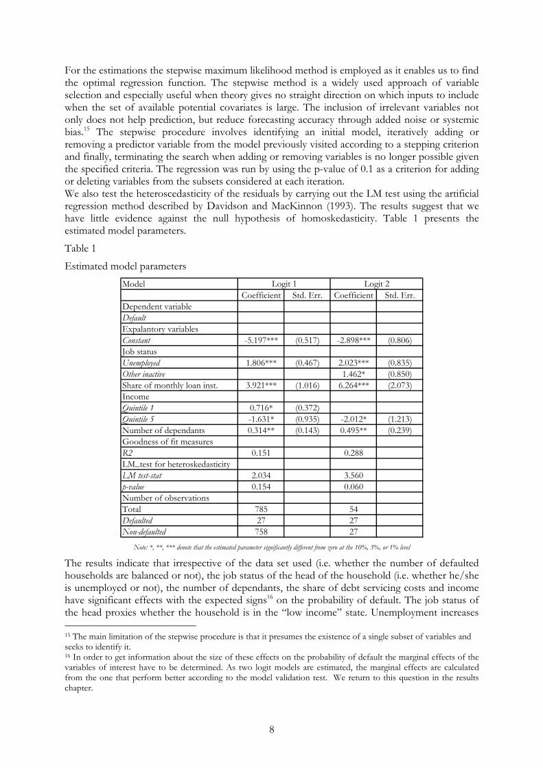
Table 1

Estimated model parameters Model

Coefficient Std. Err. Coefficient Std. Err.Dependent variableDefaultExpalantory variablesConstant -5.197*** (0.517) -2.898*** (0.806)Job statusUnemployed 1.806*** (0.467) 2.023*** (0.835)Other inactive 1.462* (0.850)Share of monthly loan inst. 3.921*** (1.016) 6.264*** (2.073)Income Quintile 1 0.716* (0.372)Quintile 5 -1.631* (0.935) -2.012* (1.213)Number of dependants 0.314** (0.143) 0.495** (0.239)Goodness of fit measuresR2 0.151 0.288LM_test for heteroskedasticityLM test-stat 2.034 3.560p-value 0.154 0.060Number of observationsTotal 785 54Defaulted 27 27Non-defaulted 758 27

Logit 1 Logit 2

Note: *, **, *** denote that the estimated parameter significantly different from zero at the 10%, 5%, or 1% level

The results indicate that irrespective of the data set used (i.e. whether the number of defaulted households are balanced or not), the job status of the head of the household (i.e. whether he/she is unemployed or not), the number of dependants, the share of debt servicing costs and income have significant effects with the expected signs16 on the probability of default. The job status of the head proxies whether the household is in the “low income” state. Unemployment increases 15 The main limitation of the stepwise procedure is that it presumes the existence of a single subset of variables and seeks to identify it. 16 In order to get information about the size of these effects on the probability of default the marginal effects of the variables of interest have to be determined. As two logit models are estimated, the marginal effects are calculated from the one that perform better according to the model validation test. We return to this question in the results chapter.

9

the likelihood of having payment problems as this is the main source of unexpected changes in income. The relationship between payment problems and the number of dependants is also positive as the larger the family, the more it is exposed to expense shocks. The effect of income on the default probability is also evident as being in higher income quintiles decreases the probability of payment problems. In addition to its traditional channels, the “income effect” also exerts its effect through the debt servicing cost ratio, i.e. a fall in disposable income increases the debt servicing cost ratio. If this ratio is high, it increases the likelihood of payment problems as it prevents the accumulation of reserves and makes these households to be more exposed to the negative consequences of rising debt servicing, basic living costs or income loss.

2.3.2 The neural network approach As an alternative of the logit, we use artificial neural networks (ANN) to model default probability. The main advantage of artificial network models is the ability to deal with problems in which relationships among variables and the underlying nonlinearities are not well known. For a detailed description of neural networks, their main attributes, architectures and workings see Sargent (1993) and Beltratti et al. (1996). Here we give a brief overview about the simple network model used.

Model description The network has three basic components: neurons, an interconnection “rule” and a learning scheme. Depending on its complexity a network consists of one input layer, one or more intermediate or hidden layers, and one output layer.

The key element of the network is the neuron that is composed of two parts a combination and an activation function. The combination function computes the net input of the neuron that is usually the weighted sum of the inputs while the activation function is a function that generates output given the net input.

We begin with the specification of the combination function for the output layer as

( )6.2 j

q

jj ay ∑

=

+=1

0 θθ

where y is the output (default, non-default), ja is the hidden node value for node j , jθ ’s are the node weights and q is the number of hidden nodes. Constraining the output of a neuron to be within the 0 and 1 interval is a standard procedure. For this purpose we use the sigmoid function.17

The ja ’s are the values at hidden node j , and are expressed as follows:

( )7.2 ⎟⎟⎠

⎞⎜⎜⎝

⎛= ∑

=

jq

iijij xwSa

1

if S has a sigmoid form, then

( )8.2⎟⎟

⎠

⎞

⎜⎜

⎝

⎛⎟⎟⎠

⎞⎜⎜⎝

⎛⎟⎟⎠

⎞⎜⎜⎝

⎛−+= ∑

=

jq

iijij xwa

1exp1/1

17 Other functions such as the logistic are also suitable.

10

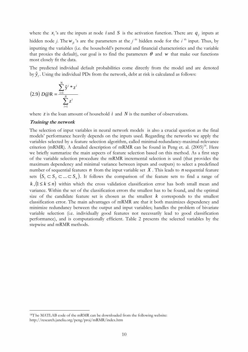
where the ix ’s are the inputs at node i and S is the activation function. There are jq inputs at hidden node j. The jiw ’s are the parameters at the j th hidden node for the i th input. Thus, by inputting the variables (i.e. the household’s personal and financial characteristics and the variable that proxies the default), our goal is to find the parameters θ and w that make our functions most closely fit the data.

The predicted individual default probabilities come directly from the model and are denoted by ty . Using the individual PDs from the network, debt at risk is calculated as follows:

( )9.2∑

∑

=

== N

i

i

i

z

zD

1

N

1i

i *y@R

where z is the loan amount of household i and N is the number of observations.

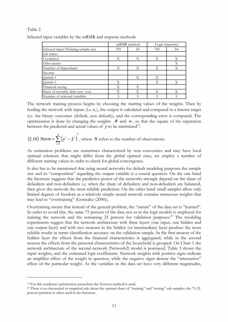
Training the network The selection of input variables in neural network models is also a crucial question as the final models’ performance heavily depends on the inputs used. Regarding the networks we apply the variables selected by a feature selection algorithm, called minimal-redundancy-maximal-relevance criterion (mRMR). A detailed description of mRMR can be found in Peng et. al. (2005)18. Here we briefly summarize the main aspects of feature selection based on this method. As a first step of the variable selection procedure the mRMR incremental selection is used (that provides the maximum dependency and minimal variance between inputs and outputs) to select a predefined number of sequential features n from the input variable set X . This leads to n sequential feature sets ( )nSSS ⊂⊂⊂ ...21 . It follows the comparison of the feature sets to find a range of k , ( )nk ≤≤1 within which the cross validation classification error has both small mean and variance. Within the set of the classification errors the smallest has to be found, and the optimal size of the candidate feature set is chosen as the smallest k corresponds to the smallest classification error. The main advantages of mRMR are that it both maximizes dependency and minimize redundancy between the output and input variables; handles the problem of bivariate variable selection (i.e. individually good features not necessarily lead to good classification performance), and is computationally efficient. Table 2 presents the selected variables by the stepwise and mRMR methods.

18T he MATLAB code of the mRMR can be downloaded from the following website: http://research.janelia.org/peng/proj/mRMR/index.htm

11

Table 2

Selected input variables by the mRMR and stepwise methods

Selected input\Training sample size 785 54 785 54Job statusUnemployed X X X XOther inactive XNumber of dependants X X X XIncome Quintile 1 X XQuintile 5 X X XFinancial saving X XShare of monthly debt serv. cost X X X XNumber of selected variables 5 5 5 5

Logit (stepwise)mRMR method

The network training process begins by choosing the starting values of the weights. Then by feeding the network with inputs (i.e. ix ), the output is calculated and compared to a known target (i.e. the binary outcomes (default, non default)), and the corresponding error is computed. The optimization is done by changing the weights θ and w , so that the square of the separation between the predicted and actual values of y to be minimized19:

( )10.2 ( )2

1

ˆ∑=

−=N

i

ii yyNorm , where N refers to the number of observations.

As estimation problems are sometimes characterized by non convexities and may have local optimal solutions that might differ from the global optimal ones, we employ a number of different starting values in order to check for global convergence.

It also has to be mentioned that using neural networks for default modeling purposes the sample size and its “composition” regarding the output variable is a crucial question. On the one hand the literature suggests that the predictive power of the networks strongly depend on the share of defaulters and non-defaulters i.e. when the share of defaulters and non-defaulters are balanced, then gives the network the most reliable prediction. On the other hand small samples allow only limited degrees of freedom as a relatively simple neural network contains numerous weights that may lead to “overtraining” (Gonzalez (2000)).

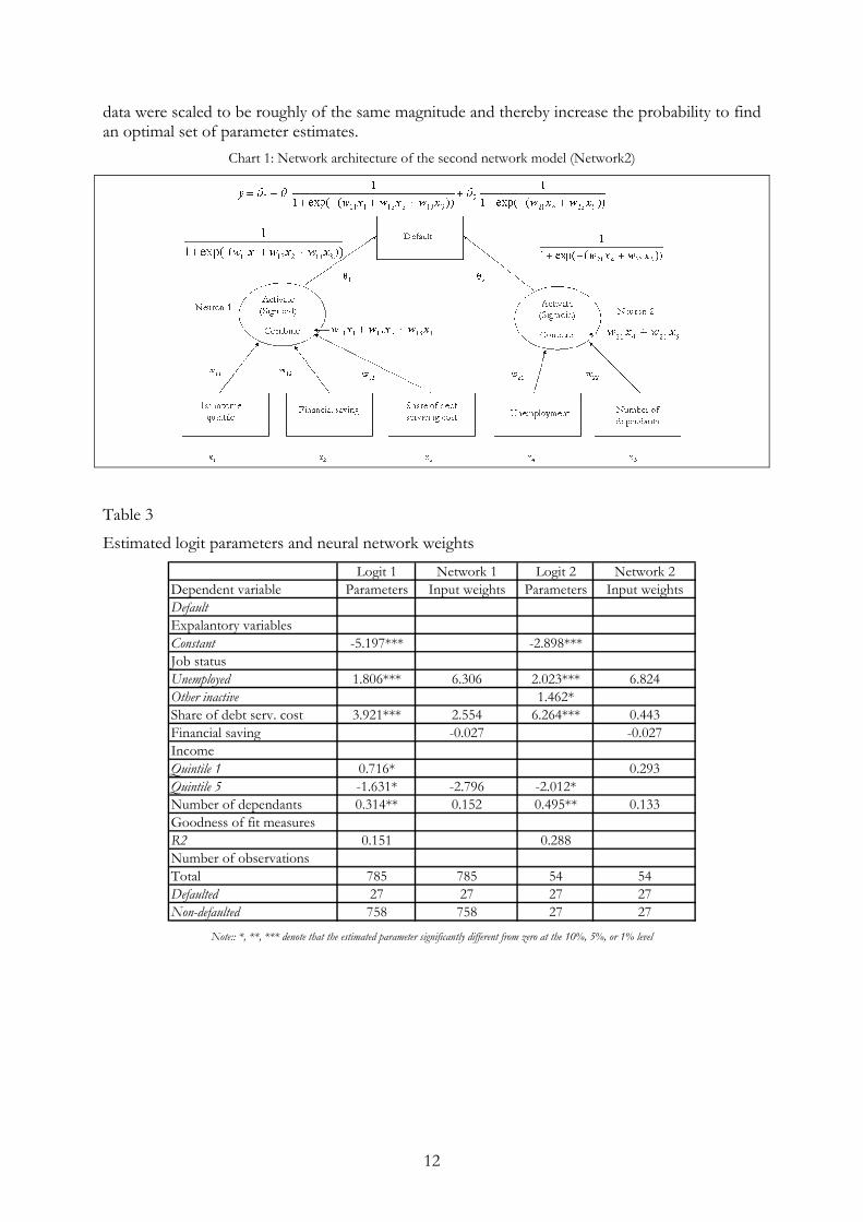
Overtraining means that instead of the general problem, the “nature” of the data set is ”learned”. In order to avoid this, the same 75 percent of the data sets as in the logit models is employed for training the network and the remaining 25 percent for validation purposes.20 The modeling experiments suggest that the network architecture with three layers (one input, one hidden and one output layer) and with two neurons in the hidden (or intermediate) layer produce the most reliable results in terms classification accuracy on the validation sample. In the first neuron of the hidden layer the effects from the financial characteristics is aggregated, while in the second neuron the effects from the personal characteristics of the household is grouped. On Chart 1 the network architecture of the second network (Network2) model is portrayed. Table 3 shows the input weights, and the estimated logit coefficients. Network weights with positive signs indicate an amplifier effect of the weight in question, while the negative signs denote the “attenuative” effect of the particular weight. As the variables in the data set have very different magnitudes,

19 For this nonlinear optimization procedure the Newton method is used. 20 There is no theoretical or empirical rule about the optimal share of “training” and “testing” sub samples, the 75-25 percent partition is often used in the literature.

12

data were scaled to be roughly of the same magnitude and thereby increase the probability to find an optimal set of parameter estimates.

Chart 1: Network architecture of the second network model (Network2)

Table 3

Estimated logit parameters and neural network weights Logit 1 Network 1 Logit 2 Network 2

Dependent variable Parameters Input weights Parameters Input weightsDefaultExpalantory variablesConstant -5.197*** -2.898***Job statusUnemployed 1.806*** 6.306 2.023*** 6.824Other inactive 1.462*Share of debt serv. cost 3.921*** 2.554 6.264*** 0.443Financial saving -0.027 -0.027Income Quintile 1 0.716* 0.293Quintile 5 -1.631* -2.796 -2.012*Number of dependants 0.314** 0.152 0.495** 0.133Goodness of fit measuresR2 0.151 0.288Number of observationsTotal 785 785 54 54Defaulted 27 27 27 27Non-defaulted 758 758 27 27

Note:: *, **, *** denote that the estimated parameter significantly different from zero at the 10%, 5%, or 1% level

13

2.4 Model validation and selection As we have four different models (two logits and two networks), validating them is necessary in order to select the best ones for further analysis. The main purpose of the application of sound model validation techniques is to reduce model risk. Comparing two or more credit risk models irrespective of the particular performance measures used, there are at least four rules that should be considered. First, when performance measures are sample dependent, the different models have to be compared on the same dataset.21 Second, samples should be representative of the general population of obligors. Third, the data sets used for model estimations and validations should differ. Fourth, robustness of the employed performance measures has to be determined by calculating confidence intervals.

The literature of model selection and validation techniques is quite broad, for a detailed description see Burnham and Anderson (1998). Here we limit our attention to the most commonly used validation technique, the receiver operating characteristic (ROC) method.22 Its use is a standard part of establishing model performance in accordance with the New Capital Accords of the Basel Committee on Banking Supervision. Here we briefly explain the ROC curve concept by using Sobehart and Keenan’s (2001) notation, then we present our model validation results based on the ROC concept.

2.4.1 The ROC curve concept When the classification accuracy of a model is analyzed a cutoff value ( )C is selected in order to classify the debtors. Debtors with rating scores or PDs below the cutoff value are considered as defaulters and debtors with scores above the cutoff value are considered as non-defaulters. If the score is below the cutoff value and the debtor defaults, the classification decision was correct. If the score is above the cutoff value and the debtor does not default, the classification was also correct. Any other cases, the obligors were wrongly classified.

Employing Sobehart and Keenan’s (2001) notation, the hit rate ( )CHR is defined as follows:

( )11.2 ( ) ( )ND

CHCHR =

where ( )CH is the number of defaulters correctly predicted with cutoff value C , and ND is the total number of defaulters in the sample. The false alarm rate ( )CFAR can be expressed as follows:

( )12.2 ( ) ( )NND

CFCFAR =

21 To see this consider two default prediction models X and Y, and assume that both models are capable of sorting riskiness with perfect accuracy. Model X is applied to sample X1, where 4 percent of the observations are defaults and Y is applied to sample Y1, where 8 percent of the observations are defaults. Then we sort the samples and select a cutt-off value of the worst 4 percent of scored observations. Since the models are by assumption has perfect accuracy, the performance of model X on sample X1 is 100 percent while the performance of model Y on sample Y1 in only 50 percent at the same cut-off, indicating the model X is better than model Y because of the higher capture rate is wrong. The problem is that the selected cut-off has a different meaning in terms of sample rejection for any two samples with different number of defaults. 22 There other widely used measures are the cumulative accuracy profile (CAP) and its summary statistics, the accuracy ratio (AR), and the conditional information entropy ratio (CIER). The CAP is similar to the ROC curve concept described. The basic idea of CIER is to compare the uncertainty of the unconditional default probability of the sample (frequency of defaults), with the uncertainty of the conditional default probability.

14

where ( )CF is the number of non-defaulters incorrectly classified as defaulters, by using the cutoff value C , and NND refers to the total number of non-defaulters in the sample.

For all the cutoff values that are contained in the range of the scores the quantities of ( )CHR and ( )CFAR are calculated.

The ROC curve is the plot of ( )CHR versus ( )CFAR . The better the model’s performance, the closer the ROC curve is to the point ( )1,0 . Denoting the area below the ROC curve by A it can be calculated as follows:

( )13.2 ( ) ( )FARdFARHRA ∫=1

0

This measure is usually between 0.5 and 1.0 for rating models in practice. A perfect model would have an area below the ROC curve of 1 or 100 percent, because this means all of the defaulting observations have a default probability greater than the PDs of the remaining observations. When the value is 0.5 or 50 percent it indicates a worthless model because the defaulters are indistinguishable from the median non-defaulter. For calculating the confidence interval for A the concept of Bamber (1975) is followed. Derivations and proofs can be found in the referred article.23

2.4.2 Model validation results Calculating the area below the ROC curves, A and confidence intervals, for both the logit and the neural network models, the remaining 25 percent of the sample, the validation sample is used. In Table 4 the estimated size of the area below the ROC curve and its confidence band can be seen for the four models.24 Although the number of defaults in both samples is the same, the share of defaulters within the samples differs. Therefore only those models are comparable whose database is the same in size. It has to be noted that when judging models classification accuracy not only the size of the area below the ROC curve matters but its standard error and the range of its confidence band as well. Regarding the larger samples the logit seems to perform better. Although the area below the ROC curve is slightly smaller than in the network model (Network1), but both the standard deviation and the confidence band range is smaller. When the number of defaulters and non-defaulters is balanced, the network outperforms the logit. This result coincides with the literature that the performance of neural networks in default modeling depends on the sample share of defaulters and non-defaulters. The consequence of the validation process is that the first logit model (Logit1) and the network (Network2) are employed for further analysis.

23 It has to note, that for a good approximation of the confidence band for A by using Bamber’s method there should be at least around 50 defaults in the sample. When there are a few numbers of defaults, the normal approximation might be problematic. However, Engelmann and Tasche (2003) empirically showed that for the cases with very few defaults in the validation sample, the approximation does not lead to completely misleading results. We also check the robustness of our validation results by randomly drawing three sub portfolios. The first sub-group contains 36 defaulters and 225 non-defaulters, the second 25 defaulters and 236 non-defaulters; the third consists of 10 defaulters and 251 non-defaulters. Our results suggest that the boundaries of the confidence bands differ by about 3-6 percentage points. 24 The ROC curves of the four models can be found in the appendix.

15

Table 4

Estimated areas below the ROC curve their confidence bands ROC area Std. Err. Validation sample size (N) Non defaulted (N)

Logit1 0.820 0.032 261 252Network1 0.827 0.070 261 252

Logit2 0.796 0.050 18 9Network2 0.889 0.079 18 9

[95% Conf.Interval]

[0.697 , 0.894][0.735 , 0.978]

[0.757 , 0.883][0.690 , 0.964]

3 Results In this chapter we first determine the effects of the model variables on the probability of default by using the first logit (Logit 1) and the second network (Network 2) models, then we analyze how the PDs and debt at risk are distributed along various dimensions and determine the concentration risk. Finally we present our stress testing exercise and analyze the shock absorbing capacity of the banking system.

3.1 Marginal effects The estimation results suggested that five variables have sizeable effects on the default probability (1st and 5th income quintiles, share of debt servicing cost, number of dependants, the job status of the head of the household, and the financial saving). As the estimated coefficients give the direction but not necessarily the size of the effect the particular variable have on the probability of default the marginal effects have to be calculated. In the logit framework the marginal effect of a continuous variable can be expressed as follows:

( )14.2[ ] ( ) ( )[ ]

( )β

βββββ 2)exp(1

)exp(1x

xxxx

xyE′+

′=′Λ−′Λ=

∂∂

,where x′ is the vector of covariates

and β is the vector of estimated parameters, while25 the marginal effects from the above described network model can be calculated according to the following formula:26

( )15.2( )

2

1

1

1exp

exp

⎟⎟⎠

⎞⎜⎜⎝

⎛+⎟⎟

⎠

⎞⎜⎜⎝

⎛

⎟⎟⎠

⎞⎜⎜⎝

⎛

=∂∂

∑

∑

=

=

q

iiji

ji

q

iiji

ji

xw

wxw

xy θ

The marginal effects of the model variables are presented in Table 5.

25 It has to mention that the use of this formula for computing the marginal effect a dummy variable is not appropriate; however the derivative approximation is often accurate. 26 The derivation can be found in Appendix 2.

16

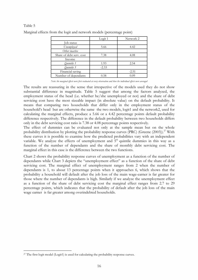
Table 5

Marginal effects from the logit and network models (percentage point) Logit 1 Network 2

Job statusUnemployed 5.66 4.42

Other inactiveShare of debt serv. cost 7.38 4.08

Income Quintile 1 1.93 2.54Quintile 5 -2.33

Financial saving -2.51Number of dependants 0.58 0.09

Note: the marginal effects were first evaluated at every observation and then the individual effects were averaged The results are reassuring in the sense that irrespective of the models used they do not show substantial difference in magnitude. Table 5 suggest that among the factors analyzed, the employment status of the head (i.e. whether he/she unemployed or not) and the share of debt servicing cost have the most sizeable impact (in absolute value) on the default probability. It means that comparing two households that differ only in the employment status of the household’s head but are otherwise the same the two models, logit1 and the network2, used for calculating the marginal effects, produce a 5.66 or a 4.42 percentage points default probability difference respectively. The difference in the default probability between two households differs only in the debt servicing cost ratio is 7.38 or 4.08 percentage points respectively. The effect of dummies can be evaluated not only at the sample mean but on the whole probability distribution by plotting the probability response curves (PRC) (Greene (2003)).27 With these curves it is possible to examine how the predicted probabilities vary with an independent variable. We analyze the effects of unemployment and 5th quintile dummies in this way as a function of the number of dependants and the share of monthly debt servicing cost. The marginal effect in this case is the difference between the two functions.

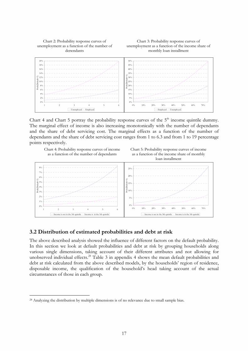
Chart 2 shows the probability response curves of unemployment as a function of the number of dependants while Chart 3 depicts the “unemployment effect” as a function of the share of debt servicing cost. The marginal effect of unemployment ranges from 2 when the number of dependants is 1, to about 13 percentage points when it approaches 6, which shows that the probability a household will default after the job loss of the main wage-earner is far greater for those where the number of dependants is high. Similarly if we analyze the unemployment effect as a function of the share of debt servicing cost the marginal effect ranges from 2.7 to 29 percentage points, which indicates that the probability of default after the job loss of the main wage earner is far greater among overindebted households.

27 The first logit model (Logit1) is used for calculating the probability response curves.

17

0%

2%

4%

6%

8%

10%

12%

14%

16%

18%

20%

1 2 3 4 5 6

Prob

(Def

ault=

1)

Unemployed Employed

0%

5%

10%

15%

20%

25%

30%

35%

40%

45%

50%

0% 10% 20% 30% 40% 50% 60% 70%

Prob

(Def

ault=

1)

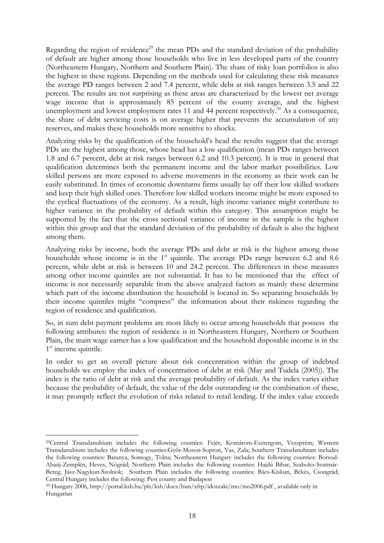
Employed Unemployed Chart 4 and Chart 5 portray the probability response curves of the 5th income quintile dummy. The marginal effect of income is also increasing monotonically with the number of dependants and the share of debt servicing cost. The marginal effects as a function of the number of dependants and the share of debt servicing cost ranges from 1 to 6.3 and from 1 to 19 percentage points respectively.

0%

1%

2%

3%

4%

5%

6%

7%

8%

1 2 3 4 5 6

Prob

(Def

ault=

1)

Income is not in the 5th quintile Income is in the 5th quintile

0%

5%

10%

15%

20%

25%

0% 10% 20% 30% 40% 50% 60% 70%

Prob

(Def

ault=

1)

Income is not in the 5th quintile Income is in the 5th quintile 3.2 Distribution of estimated probabilities and debt at risk The above described analysis showed the influence of different factors on the default probability. In this section we look at default probabilities and debt at risk by grouping households along various single dimensions, taking account of their different attributes and not allowing for unobserved individual effects.28 Table 3 in appendix 4 shows the mean default probabilities and debt at risk calculated from the above described models, by the households’ region of residence, disposable income, the qualification of the household’s head taking account of the actual circumstances of those in each group.

28 Analyzing the distribution by multiple dimensions is of no relevance due to small sample bias.

Chart 2: Probability response curves of unemployment as a function of the number of

dependants

Chart 3: Probability response curves of unemployment as a function of the income share of

monthly loan installment

Chart 4: Probability response curves of income as a function of the number of dependants

Chart 5: Probability response curves of income as a function of the income share of monthly

loan installment

18

Regarding the region of residence29 the mean PDs and the standard deviation of the probability of default are higher among those households who live in less developed parts of the country (Northeastern Hungary, Northern and Southern Plain). The share of risky loan portfolios is also the highest in these regions. Depending on the methods used for calculating these risk measures the average PD ranges between 2 and 7.4 percent, while debt at risk ranges between 3.5 and 22 percent. The results are not surprising as these areas are characterized by the lowest net average wage income that is approximately 85 percent of the county average, and the highest unemployment and lowest employment rates 11 and 44 percent respectively.30 As a consequence, the share of debt servicing costs is on average higher that prevents the accumulation of any reserves, and makes these households more sensitive to shocks.

Analyzing risks by the qualification of the household’s head the results suggest that the average PDs are the highest among those, whose head has a low qualification (mean PDs ranges between 1.8 and 6.7 percent, debt at risk ranges between 6.2 and 10.3 percent). It is true in general that qualification determines both the permanent income and the labor market possibilities. Low skilled persons are more exposed to adverse movements in the economy as their work can be easily substituted. In times of economic downturns firms usually lay off their low skilled workers and keep their high skilled ones. Therefore low skilled workers income might be more exposed to the cyclical fluctuations of the economy. As a result, high income variance might contribute to higher variance in the probability of default within this category. This assumption might be supported by the fact that the cross sectional variance of income in the sample is the highest within this group and that the standard deviation of the probability of default is also the highest among them.

Analyzing risks by income, both the average PDs and debt at risk is the highest among those households whose income is in the 1st quintile. The average PDs range between 6.2 and 8.6 percent, while debt at risk is between 10 and 24.2 percent. The differences in these measures among other income quintiles are not substantial. It has to be mentioned that the effect of income is not necessarily separable from the above analyzed factors as mainly these determine which part of the income distribution the household is located in. So separating households by their income quintiles might “compress” the information about their riskiness regarding the region of residence and qualification.

So, in sum debt payment problems are most likely to occur among households that possess the following attributes: the region of residence is in Northeastern Hungary, Northern or Southern Plain, the main wage earner has a low qualification and the household disposable income is in the 1st income quintile.

In order to get an overall picture about risk concentration within the group of indebted households we employ the index of concentration of debt at risk (May and Tudela (2005)). The index is the ratio of debt at risk and the average probability of default. As the index varies either because the probability of default, the value of the debt outstanding or the combination of these, it may promptly reflect the evolution of risks related to retail lending. If the index value exceeds

29Central Transdanubium includes the following counties: Fejér, Komárom-Esztergom, Veszprém; Western Transdanubium includes the following counties:Győr-Moson-Sopron, Vas, Zala; Southern Transdanubium includes the following counties: Baranya, Somogy, Tolna; Northeastern Hungary includes the following counties: Borsod-Abaúj-Zemplén, Heves, Nógrád; Northern Plain includes the following counties: Hajdú Bihar, Szabolcs-Szatmár-Bereg, Jász-Nagykun-Szolnok; Southern Plain includes the following counties: Bács-Kiskun, Békés, Csongrád; Central Hungary includes the following: Pest county and Budapest 30 Hungary 2006, http://portal.ksh.hu/pls/ksh/docs/hun/xftp/idoszaki/mo/mo2006.pdf , available only in Hungarian

19

one it indicates that debt is concentrated among risky households, while values less than or equal to one imply that the risk concentration is not substantial.31

The values of the concentration index are 1.37 and 1.36 in the case of the logit and the network models, while 3.07 by using the non-model based framework with original income data and 2.59 by taking into account the income distortion. The results suggest that regardless of the methods used for calculating the concentration index, a substantial part of the loan portfolio is owed by potentially risky households, which is unfavorable from a financial stability point of view. Risks are somewhat mitigated by the fact that a substantial part of risky debt is comprised of mortgage loans, which are able to provide considerable security for banks in the case of default. 3.3 The stress testing exercise Stress tests are tools for analyzing the shock absorbing capacity of the banking system to adverse macroeconomic events. With stress tests we can judge whether the banking system acts as a “stabilizer” in the economy; whether it is able to absorb shocks and mitigate the negative consequences of business cycle fluctuations or more serious adverse economic events. The key aspects of stress testing are to identify the source of risks, the channels through which they are transmitted and measure their effects on the financial system. From households’ credit risk point of view two main sources of risks can be considered that have a greater significance: declining employment, and fluctuating exchange and interest rates (i.e. risk premium shock) as a consequence of the worsening domestic macro fundamentals which effect might be amplified by the changing global investment climate.32 The main consequence of the first is the declining disposable income, while the impact of the second on household credit risk develops through the rising cost of debt servicing (i.e. foreign currency finance of households make their balance sheet position sensitive to exchange rate fluctuations as they do not possess with natural hedge). Regarding the risk transmission channels three can be detected through which the banking activity is principally affected: the credit risk, the income generation risk and liquidity risk channels. Liquidity risk might arise through the credit risk channel as a result of the worsening profitability related to household lending, that might lower market confidence and raise the cost of external finance. Banks are faced with income generation risk when the operational environment becomes unfavorable that reduces banks’ capacity to generate income (especially net interest and fee income, a substantial proportion of which is related to household lending). Finally, increasing write offs reflects the deterioration in households’ payment ability. In this paper we separately analyzed the effects of the most severe employment and risk premium shock scenarios on banks’ capital adequacy and among the risk transmission channels only the credit risk channel is taken into account. However the shocks in question might occur simultaneously and their combination might have a greater impact than each of the individual shocks alone. As our simulations are static we have to take some simplifying assumptions. First, we presume that as a result of the shocks neither the volume nor the composition of household consumption

31 For a better understanding of this concept we present a similar example as May and Tudela (2005). Suppose that there are two households A and B. Household A has a debt of 1000 000 HUF and B has a debt of 500 000 HUF. Suppose that each household has an equal default probability (10 percent). Then the total debt at risk is 0.1*1000 000+0.1*500 000=150 000 HUF that is 10 percent of the total debt outstanding and the mean PD is 10 percent. Suppose instead that household A has a 15 percent probability of having payment problems, while household B has a PD of 5 percent. In this case the debt at risk is 0.15*1000 000+0.05*500 000= 175 000 HUF and the share of risky debt is 11.6 percent that is higher than in the previous case. The mean probability of default is still 10 percent. The index of concentration of debt at risk in the former case (i.e. PDs were equal) is 1 while in the latter case (i.e. PDs differ) it is equal to 1.16 since the household with the larger amount of debt is now more risky. 32 Probabilities were not assigned to the occurrence of the various scenarios. It is the task of future research.

20

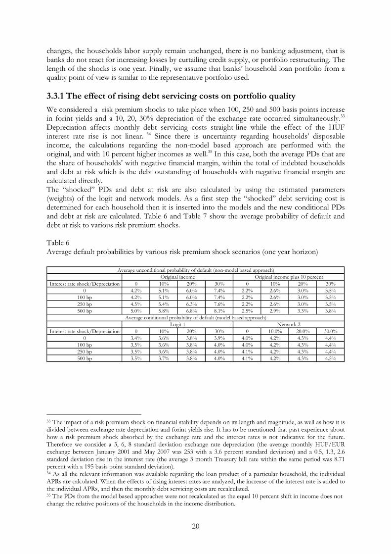
changes, the households labor supply remain unchanged, there is no banking adjustment, that is banks do not react for increasing losses by curtailing credit supply, or portfolio restructuring. The length of the shocks is one year. Finally, we assume that banks’ household loan portfolio from a quality point of view is similar to the representative portfolio used. 3.3.1 The effect of rising debt servicing costs on portfolio quality We considered a risk premium shocks to take place when 100, 250 and 500 basis points increase in forint yields and a 10, 20, 30% depreciation of the exchange rate occurred simultaneously.33 Depreciation affects monthly debt servicing costs straight-line while the effect of the HUF interest rate rise is not linear. 34 Since there is uncertainty regarding households’ disposable income, the calculations regarding the non-model based approach are performed with the original, and with 10 percent higher incomes as well.35 In this case, both the average PDs that are the share of households’ with negative financial margin, within the total of indebted households and debt at risk which is the debt outstanding of households with negative financial margin are calculated directly. The “shocked” PDs and debt at risk are also calculated by using the estimated parameters (weights) of the logit and network models. As a first step the “shocked” debt servicing cost is determined for each household then it is inserted into the models and the new conditional PDs and debt at risk are calculated. Table 6 and Table 7 show the average probability of default and debt at risk to various risk premium shocks. Table 6 Average default probabilities by various risk premium shock scenarios (one year horizon)

Interest rate shock/Depreciation 0 10% 20% 30% 0 10% 20% 30%0 4.2% 5.1% 6.0% 7.4% 2.2% 2.6% 3.0% 3.5%

100 bp 4.2% 5.1% 6.0% 7.4% 2.2% 2.6% 3.0% 3.5%250 bp 4.5% 5.4% 6.3% 7.6% 2.2% 2.6% 3.0% 3.5%500 bp 5.0% 5.8% 6.8% 8.1% 2.5% 2.9% 3.3% 3.8%

Interest rate shock/Depreciation 0 10% 20% 30% 0 10.0% 20.0% 30.0%0 3.4% 3.6% 3.8% 3.9% 4.0% 4.2% 4.3% 4.4%

100 bp 3.5% 3.6% 3.8% 4.0% 4.0% 4.2% 4.3% 4.4%250 bp 3.5% 3.6% 3.8% 4.0% 4.1% 4.2% 4.3% 4.4%500 bp 3.5% 3.7% 3.8% 4.0% 4.1% 4.2% 4.3% 4.5%

Average conditional probability of default (model based approach)Logit 1 Network 2

Average unconditional probability of default (non-model based approach)Original income Original income plus 10 percent

33 The impact of a risk premium shock on financial stability depends on its length and magnitude, as well as how it is divided between exchange rate depreciation and forint yields rise. It has to be mentioned that past experience about how a risk premium shock absorbed by the exchange rate and the interest rates is not indicative for the future. Therefore we consider a 3, 6, 8 standard deviation exchange rate depreciation (the average monthly HUF/EUR exchange between January 2001 and May 2007 was 253 with a 3.6 percent standard deviation) and a 0.5, 1.3, 2.6 standard deviation rise in the interest rate (the average 3 month Treasury bill rate within the same period was 8.71 percent with a 195 basis point standard deviation). 34 As all the relevant information was available regarding the loan product of a particular household, the individual APRs are calculated. When the effects of rising interest rates are analyzed, the increase of the interest rate is added to the individual APRs, and then the monthly debt servicing costs are recalculated. 35 The PDs from the model based approaches were not recalculated as the equal 10 percent shift in income does not change the relative positions of the households in the income distribution.

21

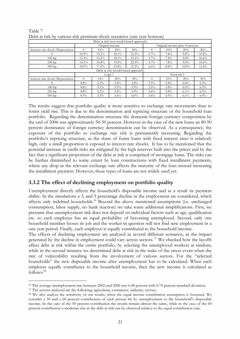
Table 7 Debt at risk by various risk premium shock scenarios (one year horizon)

Interest rate shock/Depreciation 0 10% 20% 30% 0 10% 20% 30%0 12.9% 15.5% 18.1% 21.5% 5.7% 7.8% 9.0% 10.6%

100 bp 13.2% 15.5% 18.1% 21.5% 5.7% 7.8% 9.0% 10.6%250 bp 14.1% 16.4% 19.0% 22.4% 5.7% 7.8% 9.0% 10.6%500 bp 14.9% 17.2% 19.8% 23.2% 6.6% 8.8% 10.0% 11.6%

Interest rate shock/Depreciation 0 10% 20% 30% 0 10% 20% 30%0 4.8% 5.1% 5.4% 5.8% 5.5% 5.8% 6.0% 6.3%

100 bp 4.8% 5.1% 5.5% 5.9% 5.5% 5.8% 6.0% 6.3%250 bp 4.8% 5.2% 5.5% 5.9% 5.6% 5.8% 6.1% 6.3%500 bp 4.9% 5.3% 5.6% 6.0% 5.6% 5.9% 6.1% 6.4%

Logit 1 Network 2

Debt at risk (non-model based approach)Original income Original income plus 10 percent

Debt at risk (model based approach)

The results suggest that portfolio quality is more sensitive to exchange rate movements than to forint yield rise. This is due to the denomination and repricing structure of the household loan portfolio. Regarding the denomination structure the domestic-foreign currency composition by the end of 2006 was approximately 50-50 percent. However in the case of the new loans an 80-90 percent dominance of foreign currency denomination can be observed. As a consequence, the exposure of the portfolio to exchange rate risk is permanently increasing. Regarding the portfolio’s repricing structure, as the share of forint loans with fixed interest rates is relatively high, only a small proportion is exposed to interest rate shocks. It has to be mentioned that the potential increase in credit risks are mitigated by the high reserves built into the prices and by the fact that a significant proportion of the debt at risk is comprised of mortgage loans. The risks can be further diminished to some extent by loan constructions with fixed installment payments, where any drop in the relevant exchange rate affects the maturity of the loan instead increasing the installment payment. However, these types of loans are not widely used yet. 3.3.2 The effect of declining employment on portfolio quality Unemployment directly affects the household’s disposable income and as a result its payment ability. In the simulations a 3, and 5 percentage decline in the employment are considered, which affects only indebted households.36 Beyond the above mentioned assumptions (i.e. unchanged consumption, labor supply, no bank reaction) we take some additional simplifications. First, we presume that unemployment risk does not depend on individual factors such as age, qualification etc. so each employee has an equal probability of becoming unemployed. Second, only one household member looses its job and the worker in question will not find new employment in a one year period. Finally, each employee is equally contributed to the household income. The effects of declining employment are analyzed in several different scenarios, as the impact generated by the decline in employment could vary across sectors. 37 We checked how the layoffs affect debt at risk within the entire portfolio, by selecting the unemployed workers at random, while in the second instance we determined debt at risk in the wake of the stress event when the rate of vulnerability resulting from the involvement of various sectors. For the “selected households” the new disposable income after unemployment has to be calculated. When each employee equally contributes to the household income, then the new income is calculated as follows:38

36 The average unemployment rate between 2002 and 2006 was 6.48 percent with 0.74 percent standard deviation. 37 The sectors analyzed are the following: agriculture, commerce, industry, service. 38 We also analyze the sensitivity of our results, when the equal income contribution assumption is loosened. We consider a 50 and a 60 percent contribution of each person hit by unemployment to the household’s disposable income. In the case of the 50 percent contribution the results remain almost the same, while in the case of the 60 percent contribution a moderate rise in the debt at risk can be observed relative to the equal contribution case.

22

( )1.3 ( ) aidunempnnyyn i

i

ii _1 +−⎟⎟

⎠

⎞⎜⎜⎝

⎛=

,where yn is the new income, n is the number of employees of household i, and unemp_aid is the dole.

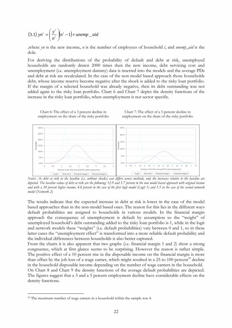
For deriving the distributions of the probability of default and debt at risk, unemployed households are randomly drawn 2000 times then the new income, debt servicing cost and unemployment (i.e. unemployment dummy) data is inserted into the models and the average PDs and debt at risk are recalculated. In the case of the non model based approach those households debt, whose income reserve become negative after the shock is added to the risky loan portfolio. If the margin of a selected household was already negative, then its debt outstanding was not added again to the risky loan portfolio. Chart 6 and Chart 7 depict the density functions of the increase in the risky loan portfolio, when unemployment is not sector specific.

0.0%

5.0%

10.0%

15.0%

20.0%

25.0%

30.0%

0 0.5 1 1.5 2 2.5 3 3.5 4

Increase in the risky loan portfolio (percentage point)

Prob

abili

ty

Logit 1 Network 2 Financial margin 1 Financial margin 2

0.0%

5.0%

10.0%

15.0%

20.0%

25.0%

0 0.5 1 1.5 2 2.5 3 3.5 4 4.5 5 5.5 6 6.5 7 7.5

Increase in the risky loan portfolio (percentage point)

Prob

abili

ty

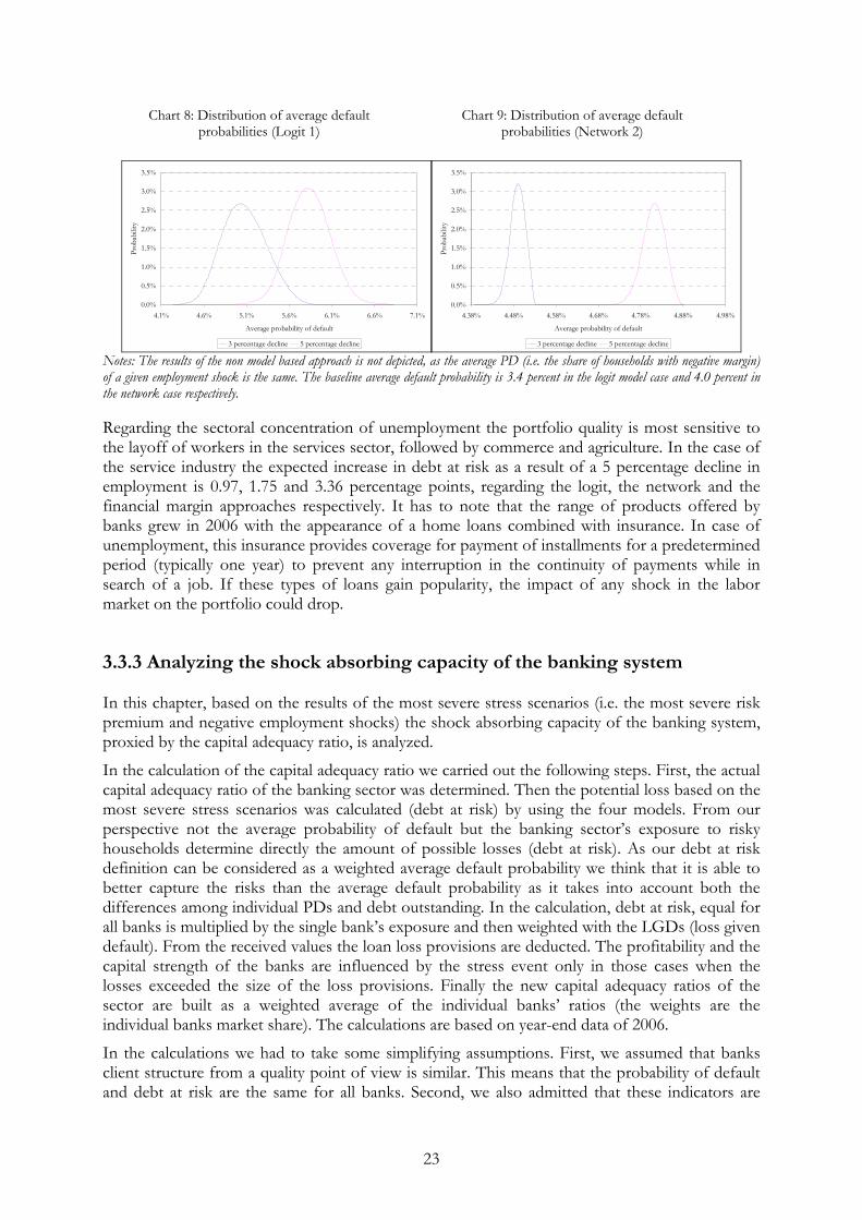
Logit 1 Network 2 Financial margin 1 Financial margin 2 Notes: As debt at risk in the baseline (i.e. without shocks) case differs across methods, only the increases relative to the baseline are depicted. The baseline values of debt at risk are the following: 12.9 and 5.7 percent in the non model based approach with original income and with a 10 percent higher income, 4.8 percent in the case of the first logit model (Logit 1) and 5.5 in the case of the second network model (Network 2) The results indicate that the expected increase in debt at risk is lower in the case of the model based approaches than in the non-model based ones. The reason for this lies in the different ways default probabilities are assigned to households in various models. In the financial margin approach the consequence of unemployment is default by assumption so the “weight” of unemployed household’s debt outstanding added to the risky loan portfolio is 1, while in the logit and network models these “weights” (i.e. default probabilities) vary between 0 and 1, so in these latter cases the “unemployment effect” is transformed into a more reliable default probability and the individual differences between households is also better captured. From the charts it is also apparent that two graphs (i.e. financial margin 1 and 2) show a strong congruence, which at first glance seems to be surprising. However the reason is rather simple. The positive effect of a 10 percent rise in the disposable income on the financial margin is more than offset by the job loss of a wage earner, which might resulted in a 25 to 100 percent39 decline in the household disposable income depending on the number of wage earners in the household. On Chart 8 and Chart 9 the density functions of the average default probabilities are depicted. The figures suggest that a 3 and a 5 percent employment decline have considerable effects on the density functions. 39 The maximum number of wage earners in a household within the sample was 4.

Chart 6: The effect of a 3 percent decline in employment on the share of the risky portfolio

Chart 7: The effect of a 5 percent decline in employment on the share of the risky portfolio

23

0.0%

0.5%

1.0%

1.5%

2.0%

2.5%

3.0%

3.5%

4.1% 4.6% 5.1% 5.6% 6.1% 6.6% 7.1%

Average probability of default

Prob

abili

ty

3 percentage decline 5 percentage decline

0.0%

0.5%

1.0%

1.5%

2.0%

2.5%

3.0%

3.5%

4.38% 4.48% 4.58% 4.68% 4.78% 4.88% 4.98%

Average probability of default

Prob

abili

ty

3 percentage decline 5 percentage decline Notes: The results of the non model based approach is not depicted, as the average PD (i.e. the share of households with negative margin) of a given employment shock is the same. The baseline average default probability is 3.4 percent in the logit model case and 4.0 percent in the network case respectively. Regarding the sectoral concentration of unemployment the portfolio quality is most sensitive to the layoff of workers in the services sector, followed by commerce and agriculture. In the case of the service industry the expected increase in debt at risk as a result of a 5 percentage decline in employment is 0.97, 1.75 and 3.36 percentage points, regarding the logit, the network and the financial margin approaches respectively. It has to note that the range of products offered by banks grew in 2006 with the appearance of a home loans combined with insurance. In case of unemployment, this insurance provides coverage for payment of installments for a predetermined period (typically one year) to prevent any interruption in the continuity of payments while in search of a job. If these types of loans gain popularity, the impact of any shock in the labor market on the portfolio could drop.

3.3.3 Analyzing the shock absorbing capacity of the banking system In this chapter, based on the results of the most severe stress scenarios (i.e. the most severe risk premium and negative employment shocks) the shock absorbing capacity of the banking system, proxied by the capital adequacy ratio, is analyzed.

In the calculation of the capital adequacy ratio we carried out the following steps. First, the actual capital adequacy ratio of the banking sector was determined. Then the potential loss based on the most severe stress scenarios was calculated (debt at risk) by using the four models. From our perspective not the average probability of default but the banking sector’s exposure to risky households determine directly the amount of possible losses (debt at risk). As our debt at risk definition can be considered as a weighted average default probability we think that it is able to better capture the risks than the average default probability as it takes into account both the differences among individual PDs and debt outstanding. In the calculation, debt at risk, equal for all banks is multiplied by the single bank’s exposure and then weighted with the LGDs (loss given default). From the received values the loan loss provisions are deducted. The profitability and the capital strength of the banks are influenced by the stress event only in those cases when the losses exceeded the size of the loss provisions. Finally the new capital adequacy ratios of the sector are built as a weighted average of the individual banks’ ratios (the weights are the individual banks market share). The calculations are based on year-end data of 2006.

In the calculations we had to take some simplifying assumptions. First, we assumed that banks client structure from a quality point of view is similar. This means that the probability of default and debt at risk are the same for all banks. Second, we also admitted that these indicators are

Chart 8: Distribution of average default probabilities (Logit 1)

Chart 9: Distribution of average default probabilities (Network 2)

24

uniform for all loan types. The only thing that implies differences among the products is the recovery ratio (1-LGD). Due to lack of reliable Hungarian data on the stream of recoveries, workout costs, and an appropriate spread for the risk of the recovery, the computation of recovery rates was not possible. Therefore we considered a 10 percent loss given default for mortgages40 and a 50 and 90 percent41 LGD for vehicle and unsecured loans, respectively. These numbers compared to the international practice are considered to be more conservative. Finally, any potential income that might be generated after 31st December 2006 was not taken into account in the calculations and we also assumed that additional capital injection is not possible.

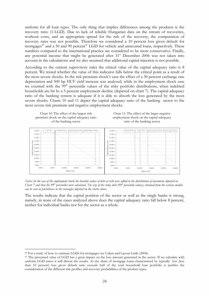
According to the current supervisory rules the critical value of the capital adequacy ratio is 8 percent. We tested whether the value of this indicator falls below the critical point as a result of the most severe shocks. In the risk premium shock’s case the effect of a 30 percent exchange rate depreciation and 500 bp HUF yield increase was analyzed, while in the employment shock case we counted with the 99th percentile values of the risky portfolio distributions, when indebted households are hit by a 5 percent employment decline (depicted on chart 7). The capital adequacy ratio of the banking system is adequate if it is able to absorb the loss generated by the most severe shocks. Charts 10 and 11 depict the capital adequacy ratio of the banking sector to the most severe risk premium and negative employment shocks.

9.60%

9.80%

10.00%

10.20%

10.40%

10.60%

10.80%

11.00%

11.20%

11.40%

11.60%

0.00% 5.00% 10.00% 15.00% 20.00% 25.00%

Debt at risk

Capi

tal a

dequ

acy

ratio

Logit 1 (6%) Network 2 (6.4%) Financial margin 2 (11.6%) Financial margin 1 (23.2%)

9.60%

9.80%

10.00%

10.20%

10.40%

10.60%

10.80%

11.00%

11.20%

11.40%

11.60%

0.00% 5.00% 10.00% 15.00% 20.00% 25.00%

Debt at risk

Capi

tal a

dequ

acy

ratio

Logit 1 (10.2%)Network 2 (7.9%) Financial margin 2 (13.7%) Financial margin 1 (21.2%)

Notes: In the case of the employment shock the baseline values of debt at risk were added to the distribution of increments depicted on Chart 7 and then the 99th percentiles were calculated. The size of the risky debt (99th percentile values), obtained from the various models can be seen in parentheses in the rectangles depicted on the charts above.

The results indicate that the capital position of the sector as well as the single banks is strong, namely, in none of the cases analyzed above does the capital adequacy ratio fall below 8 percent, neither for individual banks nor for the sector as a whole.

40 For a study of how to estimate LGDs for mortgages see Calem and Lacour-Little (2004). 41 The presumed value of LGD has a great impact on the loss amount generated in the sector. If we calculate with uniform LGD ratios it will distort the results. As the share of mortgage loans characterized by typically low (less than 10 percent) loss given default ratio exceeds half of the total household loan portfolio it justifies the consideration of the different risk profiles and recovery probabilities of the product types.

Chart 10: The effect of the largest risk premium shock on the capital adequacy ratio

of the banking sector

Chart 11: The effect of the larges negative employment shock on the capital adequacy

ratio of the banking sector

25

4 Summary and conclusion By using three different types of credit risk measurement techniques (financial margin, logit and neural network approaches) this paper investigated the main idiosyncratic determinants of household credit risk, examined whether the current state of indebtedness threatens financial stability, and by employing stress tests it analyzed the shock absorbing capacity of the banking system.

Estimation results show that the most important idiosyncratic factors of credit risk are the disposable income, the number of dependants, the share of debt servicing costs and the employment status of the head of the household. Empirical evidence suggests that effects of unemployment and income on the probability of default are monotonically increasing with the number of dependants and the share of debt servicing costs, that is, these effects are stronger among those households where the number of dependants or the share of debt servicing costs are originally high. The results also suggest that debt payment problems are most likely to occur among households living in less developed regions (i.e. Northeastern Hungary, the Northern and Southern Plain), the main wage earner has a low qualification and the household disposable income is in the 1st income quintile. The results also indicate that a substantial part of the loan portfolio is owed by potentially risky households, which is unfavorable from a financial stability point of view. However risks are somewhat mitigated by the fact that a substantial part of risky debt is comprised of mortgage loans, which are able to provide considerable security for banks in the case of default.

Regarding the stress test results of the risk premium shocks, we find that portfolio quality is more sensitive to exchange rate movements than to a forint yield rise due to the denomination and repricing structure of the household loan portfolio. In the case of the employment shock, the results suggest that employment decline has considerable effects on the size of the risky loan portfolio. Regarding the sectoral concentration of unemployment the portfolio quality is most sensitive to the layoff of workers in services, which is followed by industry, commerce and agriculture.The main finding of the study is that the banking system shows a high level of resilience both on the individual and on the aggregate level.

There are, however, some limitations; in this regard the assumption of homogenous portfolio quality, the separate shock analysis on banks capital adequacy and that we neglect to measure the effects developing through other risk transmission channels (i.e. income generation risk, and funding risk) should be mentioned. In this latter respect the size of the calculated losses might be distorted downward, but to what extent is not known. As the results provide the first set of microeconomic insights to household credit risk, drawing on these further investigations including the integrated analysis of various shocks on banks’ capital adequacy, the extension of the above analysis by using panel data, will be aimed at depicting a more refine picture of household credit risk.

26

References [1] Bamber, D., 1975, "The Area Above the Ordinal Dominance Graph and the Area below the Receiver

Operating Graph", Journal of Mathematical Psychology, 12, pp. 387-415.

[2] Beltratti, A., S. Margarita and P. Terna, 1996, "Neural Networks for Economic and Financial

Modeling," International Thompson Computer Press.

[3] Burnham, K., and D., Anderson, 1998, "Model Selection and Inference", New York: Springer, pp.

32-74.

[4] Calem, P., and M. Lacour-Little, 2004, "Risk-Based Capital Requirements for Mortgage Loans",

Journal of Banking and Finance, 28(3), pp. 647-72.

[5] Davidson, R., and J. MacKinnon, 1993, "Estimation and Inference in Econometrics", Oxford:

Oxford University Press.

[6] Drehmann, M., A. Patton and S. Sorensen, 2006, "Non-Linearities and Stress Testing"

[7] Engelmann, B., E. Hayden, and D. Tasche, 2003, "Testing Rating Accuracy", Risk, January 2003

[8] Froyland, E., and K. Larsen, 2002, "How Vulnerable are Financial Institutions to Macroeconomic

Changes? An Analysis Based on Stress Testing", Norges Bank Economic Bulletin

[9] Gonzalez, S., 2000, "Neural Networks for Macroeconomic Forecasting: A Complementary Approach to

Linear Regression Models", Working Paper 2000/7, Department of Finance, Canada

[10] Greene, W. H., 2003, "Econometric Analysis", 5th Edition, Prentice Hall.

[11] Herrala, R., and K. Kauko, 2007, "Household Loan Loss Risk in Finland - Estimations and

Simulations with Micro Data", Bank of Finland Research Discussion Papers

[12] Hoggart, G., S. Sorensen and L. Zicchino, 2005, "Stress Tests of UK Banks Using a VAR

Approach", Bank of England Working Paper, No. 282.

[13] Hungary in 2006, http://portal.ksh.hu/pls/ksh/docs/hun/xftp/idoszaki/mo/mo2006.pdf,

Publication of the Hungarian CSO, available only in Hungarian

[14] Marucci, J., and M. Quagliariello, 2005, "Is Bank Portfolio Riskiness Procyclical? Evidence from Italy

using a Vector Autoregression", University of York, Discussion Papers in Economics

[15] May, O., and M. Tudela, 2005, "When is Mortgage Indebtedness a Financial Burden to British

Households? A Dynamic Probit Approach", Bank of England Working Paper, No. 277.

[16] Peng, H., F. Long and C. Ding, (2005), “Feature selection based on mutual information: criteria of

max-dependency, max-relevance, and min-redundancy”, IEEE Transactions on Pattern Analysis and

Machine Intelligence, Vol. 27, No. 8, pp.1226-1238

[17] Report on Financial Stability, 2007,

http://english.mnb.hu/Engine.aspx?page=mnben_stabil&ContentID=9555

27

[18] Sargent, T., 1993, "Bounded Rationality in Macroeconomics", Oxford University Press, Oxford,

United Kingdom.

[19] Sobehart, J., and S. Keenan, 2002, "Measuring Default Accurately", Risk, pp. S31-S33, March

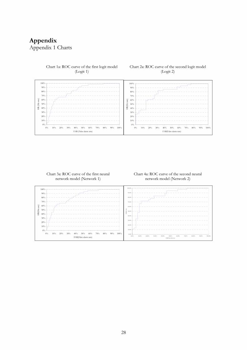
28

Appendix Appendix 1 Charts

0%

10%

20%

30%

40%

50%

60%

70%

80%

90%

100%

0% 10% 20% 30% 40% 50% 60% 70% 80% 90% 100%

FAR (False alarm rate)

HR

(Hit

rate

)

0%

10%

20%

30%

40%

50%

60%

70%

80%

90%

100%

0% 10% 20% 30% 40% 50% 60% 70% 80% 90% 100%

FAR(False alarm rate)

HR(

Hit

rate

)

0%

10%

20%

30%

40%

50%

60%

70%

80%

90%

100%

0% 10% 20% 30% 40% 50% 60% 70% 80% 90% 100%

FAR(False alarm rate)

HR(

Hit

rate

)

0.00%

10.00%

20.00%

30.00%

40.00%

50.00%

60.00%

70.00%

80.00%

90.00%

100.00%

0.00% 10.00% 20.00% 30.00% 40.00% 50.00% 60.00% 70.00% 80.00% 90.00% 100.00%

FAR(False alarm rate)

HR(

Hit

rate

)

Chart 1a: ROC curve of the first logit model (Logit 1)

Chart 2a: ROC curve of the second logit model (Logit 2)

Chart 3a: ROC curve of the first neural network model (Network 1)

Chart 4a: ROC curve of the second neural network model (Network 2)

29

Appendix 2 Derivation of the marginal effect from the network model The network model described in Section 2 is as follows:

( )a11exp

exp

1

1

10

+⎟⎟⎠

⎞⎜⎜⎝

⎛

⎟⎟⎠

⎞⎜⎜⎝

⎛

+=

∑

∑∑

=

=

= j

j

q

iiji

q

iijiq

jj

xw

xwy θθ

The marginal effect of ix can be simply acquired by deriving ( )a1 respect to ix and ix belonging to the j th neuron, that is

( )a2( ) ( )

2

1

1111

1exp

expexp1expexp

⎟⎟⎠

⎞⎜⎜⎝

⎛+⎟⎟

⎠

⎞⎜⎜⎝

⎛

⎟⎟⎠

⎞⎜⎜⎝

⎛⎟⎟⎠

⎞⎜⎜⎝

⎛⎟⎟⎠

⎞⎜⎜⎝

⎛−⎟⎟

⎠

⎞⎜⎜⎝

⎛+⎟⎟

⎠

⎞⎜⎜⎝

⎛⎟⎟⎠

⎞⎜⎜⎝

⎛

=∂∂

∑

∑∑∑∑

=

====

q

iiji

ji

q

iiji

q

iiji

q

iijiji

q

iiji

ji

xw

wxwxwxwwxw

xy θ

( )a3 after simplifications we get

( )2

1

1

1exp

exp

⎟⎟⎠

⎞⎜⎜⎝

⎛+⎟⎟

⎠

⎞⎜⎜⎝

⎛

⎟⎟⎠

⎞⎜⎜⎝

⎛

=∂∂

∑

∑

=

=

q

iiji

ji

q

iiji

ji

xw

wxw

xy θ

30

Appendix 3 Table 1 Explanatory variable set

Dummy Continuous Comment/CalculationJob status of the head of the householdEmployee XPrivate entrepreneur XUnemployed XOther inactiveQualification of the head of the householdLow XMedium XHigh XAge of the head of the household-30 X31-39 X40-49 X50-59 X60- XGender of the head of the householdMale XFemale XNumber of dependants XRegion of residenceCentral Transdanubium X Counties: Fejér, Komárom-Esztergom, VeszprémWestern Transdanubium X Counties: Győr-Moson-Sopron, Vas, ZalaSouthern Transdanubium X Counties: Baranya, Somogy, TolnaNortheastern Hungary X Counties: Borsod-Abaúj-Zemplén, Heves, NógrádNorthern Plain X Counties: Hajdú Bihar, Szabolcs-Szatmár-Bereg, Jász-Nagykun-SzolnokSouthern Plain X Counties: Bács-Kiskun, Békés, CsongrádCentral Hungary X Pest county and BudapestDisposable income Upper quintile limitsQuintile 1 X HUF 110946Quintile 2 X HUF 148597Quintile 3 X HUF 179149Quintile 4 X HUF 218790Quintile 5 XFinancial Saving X Reported value of total financial savingsReal wealth X Reported value of own cars and dwellingsShare of monthly loan inst. X Monthly debt servicing cost/monthly disposable incomeDebt to income X Debt/Yearly disposable incomeNumber of loans XLoan type XForeign (FX) XDomestic (HUF) XForeign and domestic X Table 2 Descriptive Statistics of some selected variables

Variable Mean Median Standard deviation HUF CHF EURDebt

Mortgage Loans (HUF) 4 059 049 3 000 000 3 393 147 62% 33% 5%Maturity of Mortgage Loans (Month) 150 144 86

Reported LTV 48% 45% 22%Car Purchase Loans (HUF) 1 628 867 1 500 000 851 931 31% 60% 8%

Maturity of Car Purchase Loans (Month) 48 40 30 Unsecured Loans (HUF) 408 349 200 000 712 000 92% 1% 7%

Maturity of Unsecured Loans (Month) 39 27 15Number of loan contracts 1.50 1.00 0.81

Income and wealthDisposable Income (HUF) 170 144 160 483 65 245Financial Saving (HUF) 139 484 0 521 678

Number of own cars 0.70 1.00 0.77Reported value of own cars (HUF) 835 335 220 250 1 673 700

Number of own dwellings 0.94 1.00 0.53Reported value of own dwellings (HUF) 10 962 715 10 000 000 9 103 317

ExpendituresMontly Loan Installment (HUF) 29 695 23 000 25 765

Reported income share of monthly loan installment 22% 15% 13%Calculated income share of monthly loan installment 18% 15% 14%

Consumption expenditure (HUF) 64 664 60 866 24 436Overhead expenditure (HUF) 32 118 30 265 11 812

Other household characteristicsNumber of dependants 1.31 1.00 1.29

Age of the head of the household 43 45 12

Composition of loans by denomination

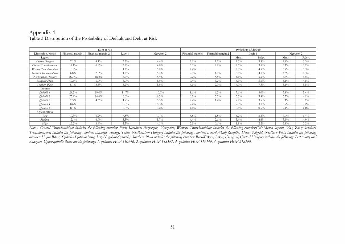
31

Appendix 4 Table 3 Distribution of the Probability of Default and Debt at Risk

Dimension/Model Financial margin1 Financial margin 2 Logit 1 Network 2 Financial margin1 Financial margin 2Region Mean Stdev. Mean Stdev.

Central Hungary 7.1% 4.1% 3.7% 4.6% 2.0% 1.2% 2.3% 3.5% 2.8% 3.3%Central Transdanubium 12.1% 6.8% 3.7% 4.6% 3.3% 2.2% 2.5% 3.5% 3.1% 3.1%Western Transdanubium 10.8% 4.7% 5.2% 2.4% 2.8% 4.5% 3.4% 3.3%Southern Transdanubium 6.8% 2.0% 4.7% 5.4% 2.9% 1.0% 3.7% 4.1% 4.5% 4.3%

Northeastern Hungary 22.0% 18.2% 5.7% 5.9% 7.2% 5.8% 4.1% 5.5% 4.4% 4.5%Northern Plain 19.6% 6.0% 5.0% 5.9% 7.4% 3.2% 4.3% 5.1% 5.1% 4.5%Southern Plain 8.1% 3.5% 5.2% 5.9% 4.1% 2.0% 4.7% 7.5% 5.1% 5.5%

IncomeQuintile 1 24.2% 19.0% 11.7% 10.0% 8.6% 6.2% 7.6% 8.0% 7.8% 5.4%Quintile 2 25.9% 14.6% 6.0% 6.5% 6.2% 3.3% 3.3% 3.8% 3.7% 4.1%Quintile 3 7.3% 4.6% 4.9% 5.3% 2.4% 1.4% 2.9% 3.5% 3.1% 3.1%Quintile 4 8.6% 5.0% 5.3% 2.4% 2.9% 3.1% 3.2% 3.2%Quintile 5 8.1% 0.8% 3.2% 1.4% 0.5% 0.5% 2.1% 1.8%

QualificationLow 10.3% 6.2% 7.3% 7.7% 4.5% 1.8% 6.2% 8.4% 6.7% 6.4%

Medium 12.4% 6.9% 5.3% 5.7% 4.4% 2.6% 3.4% 4.6% 3.9% 4.0%High 15.5% 1.4% 2.2% 4.1% 3.1% 0.6% 1.8% 2.2% 2.8% 2.2%

Logit 1 Network 2Probablity of defaultDebt at risk

Notes: Central Transdanubium includes the following counties: Fejér, Komárom-Esztergom, Veszprém; Western Transdanubium includes the following counties:Győr-Moson-Sopron, Vas, Zala; Southern Transdanubium includes the following counties: Baranya, Somogy, Tolna; Northeastern Hungary includes the following counties: Borsod-Abaúj-Zemplén, Heves, Nógrád; Northern Plain includes the following counties: Hajdú Bihar, Szabolcs-Szatmár-Bereg, Jász-Nagykun-Szolnok; Southern Plain includes the following counties: Bács-Kiskun, Békés, Csongrád; Central Hungary includes the following: Pest county and Budapest. Upper quintile limits are the following: 1. quintile: HUF 110946, 2. quintile: HUF 148597, 3. quintile: HUF 179149, 4. quintile: HUF 218790.