Understanding business cycles: credit supply, household

i

Understanding business cycles: credit supply,

household debt and financial crises in Portugal

Ricardo Filipe Pereira Santos

Dissertation presented as partial requirement for obtaining

the Master’s degree in Statistics and Information

Management

i

NOVA Information Management School

Instituto Superior de Estatística e Gestão de Informação

Universidade Nova de Lisboa

UNDERSTANDING BUSINESS CYCLES: CREDIT SUPPLY, HOUSEHOLD

DEBT AND FINANCIAL CRISES IN PORTUGAL

by

Ricardo Filipe Pereira Santos

Dissertation presented as partial requirement for obtaining the Master’s degree in Statistics

Information Management, with a specialization in Risk Management

Advisor / Co Advisor: Professor Dr. Rui Gonçalves, PhD

November 2019

ii

DEDICATION

To my family, for always being there for me at all times, even at a distance.

To my mother and father, for all the effort and affection they put in in providing me the best possible

options, for allowing me to get this far and so much farther in the years to come.

To my ever-little brother, to whom I try to be a reference every day, for being my reference as well,

for his hard work and determination and the great future ahead of him.

To Margarida, for all the love and support, for being the one by my side at all moments and the

reason why I’m writing these words.

To my grandmother, for being an inspiration, for her strength and determination.

The simple thought of all of you would give me the will to push forward just one more time, for so

many times, until this very moment I close another cycle and conquer one more new beginning.

iii

ACKNOWLEDGMENTS

A special thank you to Professor Rui Gonçalves, for the guidance and availability, and help me move

forward with this work. His knowledge and support were fundamental in completing this

dissertation.

iv

ABSTRACT

Throughout the last century, severe financial crises hit the financial markets, whose effects then

spread all over the world. Taking the recent example of the 2008 subprime crisis, it is now clear it had

its main drivers in excess credit supply and record household debt, which had been spiking since the

80’s and 90’s decades.

Allied to weak risk management policies and the deregulation in financial markets, along with

subprime credit concession and speculation regarding complex financial products, the households’

debt levels rose to a point that helped generate one of the greatest financial crises in history, whose

effects were felt around the globe.

From the moment these crises happened, various authors studied and analyzed the reasons behind

the events leading to them, and how they reached the magnitude to cause such an impact. Several

studies concerning households’ indebtedness and credit supply were made regarding many countries

and provide a closer look at how these indicators are related and how they react in periods marked

by financial crises as the ones described above. Some of them were able to prove that, indeed, there

is a connection not only between them, but also with financial markets liberalization and weak risk

management policies.

After establishing a relationship between credit supply and household debt, and connecting both to

business cycles, the core goal of this study is to evaluate the evolution of household debt in Portugal

since the introduction of the Euro and which factors contributed with the most impact to that same

evolution.

Our work will start with a literature review to explain the credit-driven household demand channel

concept and the dynamics implied and proceed with a statistical analysis of key indicators focusing

on explaining the behavior of household debt in Portugal. These will include a time-adjusted

correlations analysis and a linear regression model. Finally, we will present the conclusions reached

through these methods, which resulted in a good performing model composed of five independent

variables explaining the evolution of household debt to GDP in Portugal in different moments in

time, and present future study possibilities to enhance the knowledge on this topic.

KEYWORDS

Household Debt; Credit Supply; Financial Crises; Business Cycles; Financial Deregulation

v

INDEX

1. Introduction ............................................................................................................. 1

1.1. Background and Problem Identification ............................................................ 1

1.2. Research Gap & Objectives ............................................................................... 3

2. Literature review ..................................................................................................... 5

2.1. First Pillar: Credit Supply Expansions ................................................................. 5

2.1.1. The “Global Savings Glut” ........................................................................... 7

2.1.2. Rises in Income Inequality .......................................................................... 7

2.1.3. Financial Liberalization and Deregulation ................................................... 9

2.2. Second Pillar: Household Debt ........................................................................ 10

2.3. Third Pillar: Business Cycles Dynamics ............................................................. 12

3. Methodology and Results Analysis ......................................................................... 16

3.1. Data Selection and Variables Definition........................................................... 16

3.2. Descriptive Statistics ....................................................................................... 17

3.3. Four-Step Progressive Analysis ........................................................................ 21

3.4. Linear Regression Model and Results Analysis ................................................. 25

4. Conclusions and Future Investigation ..................................................................... 31

5. Bibliography ........................................................................................................... 33

6. Annexes ................................................................................................................. 36

vi

LIST OF FIGURES

Figure 2.1 – Credit-driven household demand channel: Pillar 1 ..............................................5

Figure 2.2 – Income Inequality and Household Leverage ........................................................8

Figure 2.3 – Lending from Banks, Mortgage Institutions, and Finance Companies (percentage

changes) .........................................................................................................................9

Figure 2.4 – Credit-driven household demand channel: Pillar 2 ............................................10

Figure 2.5 – Bank mortgage and non-mortgage lending to GDP, 1870–2011: Average ratio to

GDP by year for 17 countries ........................................................................................11

Figure 2.6 – Prediction Error in the Subprime-Prime Rate Spread .........................................12

Figure 2.7 – Credit-driven household demand channel: Pillar 3 ............................................13

Figure 2.8 – Household leverage ratios: Debt to disposable income .....................................13

Figure 2.9 – Household leverage and the decline in consumption.........................................14

Figure 3.1 – Household debt to GDP in Portugal ...................................................................18

Figure 3.2 – Net exports to GDP............................................................................................19

Figure 3.3 – Unemployment rate ..........................................................................................19

Figure 3.4 – Government debt to GDP ..................................................................................20

Figure 3.5 – Real investment ................................................................................................20

Figure 3.6 – Real durable consumption .................................................................................20

Figure 3.7 – Variance Inflator Factor .....................................................................................26

vii

LIST OF TABLES

Table 3.1 – Variables.............................................................................................................16

Table 3.2 – Descriptive Statistics ...........................................................................................18

Table 3.3 – Non adjusted correlation matrix .........................................................................22

Table 3.4 – One-year adjusted correlation matrix .................................................................23

Table 3.5 – Two-year adjusted correlation matrix .................................................................24

Table 3.6 – Three-year adjusted correlation matrix ..............................................................24

Table 3.7 – Three-year adjusted linear regression.................................................................27

Table 3.8 – Best correlations variables selection ...................................................................28

Table 3.9 – Best correlations linear regression ......................................................................28

viii

List of Abbreviations and Acronyms

CDO Collateralized Debt Obligations

IMF International Monetary Fund

INE Instituto Nacional de Estatística

MBS Mortgage-Backed Securities

NAFTA North American Free Trade Agreement

OPEC Organization of the Petroleum Exporting Countries

1

1. INTRODUCTION

1.1. BACKGROUND AND PROBLEM IDENTIFICATION

Credit supply and household debt were the main drivers for some of the greatest financial crises that

hit world economies throughout the last decades, whose effects then spread across the globe, and

some of those effects still remain to today.

As we take the 2008 subprime crisis as the most significant recent event in this context, Geithner

(2015) suggested that record household debt was one of the five major causes of the crisis, which,

through intricate dynamics, severely expanded the effects of a combination of factors which would

cause the financial markets to collapse.

In his work, Cottrell (2016) showed that the household credit market debt spiked in the 1980’s and

1990’s, and that this increase was first related to the loss, by the middle class, of their previous levels

of income, who recurred to household debt to maintain their lifestyle. Another crucial factor Cottrell

(2016) pointed out was the deregulation of financial markets, as a consequence of the rise of the

neoliberal policies carried out by the Reagan and Thatcher administration in the 80’s and the

adoption of the NAFTA, under the Clinton administration, in the 90’s. With the deregulation of

financial markets came credit supply expansion and speculation and, adding to the problem, more

and more complex financial instruments emerged, such as mortgage-backed securities and

collateralized debt obligations. The fact that a major part of the underlying securities composing

these instruments corresponded to debt contracted in already precarious conditions from the

debtors’ perspective and adding the fact that these products were backed by major rating agencies

at the time, often granting them triple A ratings, were key factors leading to the bubble burst that

would eventually come.

Debt secured by residential real estate was the reason why debt substantially increased in the

beginning of the twenty-first century until 2008, as proven by Brown et al. (2013). When these

products collapsed, as a combined deferred consequence of subprime credit concession and lack of

regulation, the crisis hit the markets.

Irwin (2013) stated that central bankers were aware of the bubble in the housing market being a

problem but weren’t able to predict the combination of factors that eventually aggravated it and

caused the economy to collapse.

Besides the 2008 subprime crisis, both credit supply and household debt played a key part in other

global financial crises over the last decades, which affected several countries around the world,

including Portugal. Indeed, the IMF (2017) and Drehmann et al. (2017) were able to relate sudden

increases in the household debt-to-GDP ratio with turning points in business cycles. Mian & Sufi

(2018) also reached the same conclusion.

In this study, we will analyze the household debt levels in Portugal since the beginning of the twenty

first century, more specifically the year when the Euro was introduced in the Portuguese economy,

then identifying the main variables leading to that evolution. Before that, and based on what was

mentioned so far in this work, we will establish a connection between credit supply and household

debt, then relating this relationship with turning points in business cycles in our literature review.

2

These dynamics will be analyzed by applying the concept of the credit-driven household demand

channel defined by Mian & Sufi (2018), which is a fundamental basis created by these authors to

explain these connections and was later confirmed by the IMF, which then extended the study to a

larger set of countries over the period 1950-2016. In their IMF published working paper, Alter,

Xiaochen Feng, & Valckx (2018) reached the same conclusion for this larger countries sample that, in

fact, household debt has a negative impact in GDP growth, thus establishing a reinforced connection

between both variables.

3

1.2. RESEARCH GAP & OBJECTIVES

Evaluating the intricate dynamics between credit supply, household debt and business cycles will

allow the establishment of household debt as playing a crucial role in aggravating the effects of

financial crises on an international scale. Hence, this study is important as it will apply these same

concepts to Portugal and analyze which are the factors that produce the most impact in the

evolution of household debt in the country. In doing so, it is potentially providing the future

possibility of an early pattern identification that could lead to the same abovementioned

consequences and allow pre-emptive measures to be taken beforehand.

On a first approach, the goal is to determine if there is a specific evolution pattern regarding these

cycles specifically concerning household debt, also applicable to Portugal, which could help better

understand its effects in households, financial institutions and the financial markets and, posteriorly,

potentially act in the sense of preventing or containing its effects on future periods where the same

patterns are observed.

The 2008 subprime crisis impacted several countries around the globe and irresponsible credit

concession practices, in the form of subprime loans (Demyanyk & Van Hemert, 2011), played a key

role in the events previously described. This proves that credit supply and household debt are of

paramount importance.

Similar analyses have been made regarding other countries, which proved important in the sense

that they allowed to corroborate the influence of household debt in relation to financial crises.

Żochowski & Zajączkowski (2007) analyzed household debt growth in Poland, also comparing it to

other European countries, and confirmed the connection between an increase in loans, financial

market liberalization and financial crises. Jauch & Watzka (2012) studied household debt evolution

and how it impacted the Spanish provinces in a macroeconomic perspective. Crook & Hochguertel

(2007) showed that there are implications of credit concession constraints in the evolution of

household debt through a systemic international comparison for four OECD countries (the United

States of America, Spain, Italy and the Netherlands). Later, Loberto & Zollino (2016) from the Bank of

Italy estimated an offset relation between declining bank rates on lending and shrinking credit

volumes conceded by the Italian banks, used as a measure to reduce the banks’ credit exposure,

which is an indicator that this could be a possible solution to control household debt while reducing

the banks’ risk.

This dissertation will extend that knowledge by applying it to Portugal. We will study the evolution of

household debt over the last decades and relate it with factors such as private and governmental

consumption levels, banks’ interest rate spreads and the aggravating impacts noticed on the curve of

the cycle. This could prove important for financial institutions to evaluate if they are exposed to risk

relating to a progressive increase in household debt, becoming a timely alert for them to take action.

On the other hand, this could prove a useful indicator to measure the effectiveness of the risk

policies and regulations implemented in Portugal over the past years, by concluding if household

debt and banks’ credit concession actually decreased after they were put in place. This project will

have as core goal to study and apply the concept of the credit-driven household demand channel,

defined by Mian & Sufi (2018), to Portugal and evaluate the evolution of key indicators regarding the

4

country since the beginning of the century, thus including the period leading to one of the greatest

financial crises that ever hit the world financial markets: the 2008 subprime mortgage crisis.

The concrete objectives we aim to achieve by the end of our dissertation are as follows:

- First, we will present the evolution of household debt in Portugal through a key economic

indicator throughout the period in analysis and identify if there is an observable turning point

related to the U.S. subprime crisis;

- Second, we will verify which variables are the most relevant in explaining this evolution and if

they do so in a linear way;

- Third, we will evaluate how such variables evolution throughout the period is related to

household debt in Portugal and if there are also observable patterns related to the U.S.

subprime crisis and the measures applied in its sequence;

- Finally, we aim to consider the results from our work to provide future study possibilities to

improve the available knowledge in this topic.

5

2. LITERATURE REVIEW

First of all, it is important to understand the concept of the credit-driven household demand channel

in order to establish the relationship between the three main study points we will focus on in this

literature review.

The credit-driven household demand channel is sustained by three main pillars, which relate credit

supply and household demand and, consequently, the amplified effects that these indicators’

evolution have on business cycles and financial crises. The subjacent idea is that the driver at the

origin of amplified booms and busts in the economy is related to expansions in credit supply. These

expansions, generated via different channels as we will describe later on, will represent an excess

which will trigger an increment in household demand, which will respectively translate into an

increase in household debt. Having more and easier access to credit, household demand expands

and pushes house prices in an upward direction creating bubbles. Financial institutions, seeking to

capitalize on the increase in the demand for credit, also tend to facilitate its access by the

households, which translated in some cases into the reduction of credit quality constraints,

aggravated by liberalization and deregulation in financial markets. All these factors combined have

an amplifying effect on the business cycle and can actually aggravate financial crises, as was recently

the case with the subprime mortgage crisis in 2008.

These are the facts on which the credit-driven household demand channel sets its ground. Now, we

will divide this analysis into three main sections, each one directly related to one of the three pillars,

and sustain with evidence the applicability of this concept, which will be the theoretical foundation

used as a basis in this work.

2.1. FIRST PILLAR: CREDIT SUPPLY EXPANSIONS

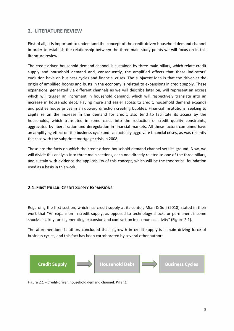
Regarding the first section, which has credit supply at its center, Mian & Sufi (2018) stated in their

work that “An expansion in credit supply, as opposed to technology shocks or permanent income

shocks, is a key force generating expansion and contraction in economic activity” (Figure 2.1).

The aforementioned authors concluded that a growth in credit supply is a main driving force of

business cycles, and this fact has been corroborated by several other authors.

Figure 2.1 – Credit-driven household demand channel: Pillar 1

6

Krishnamurthy & Muir (2017) linked adverse real outcomes to substantial losses occurring after

periods of expansion in credit supply, by studying the progress of credit spreads calculated

essentially through two measures: the risk-neutral probability of a large loss and the risk-neutral

expectation of output declines.

They concluded that the gap between higher grade and lower grade bonds spreads presents a

tendency to become smaller in periods of credit expansion occurring before a crisis. Although credit

growth and spreads are positively correlated under regular circumstances, they are negatively

correlated when calculated for the five years preceding a financial crisis. This translates into the fact

that the risk-neutral probability of a large loss for a given investor actually decreases as credit growth

expands, and they estimate that the spreads are 25% below their optimal value in pre-crises periods.

They then conclude that the combination of credit supply expansion and uncommonly low spreads is

an important factor to take into consideration when predicting crises, fact this that is sustained by

the work of Mian, Sufi, & Verner (2017a) regarding the effect of a similar tendency in credit growth

applied to an international sample dating a few decades back, until the 1970’s.

On another perspective, Jordà et al. (2016) defined the sharp increase in credit supply under the

form of real estate loans provided by banks as the main cause of the rise in credit-to-GDP ratios in

advanced economies in the past century. More specifically, they demonstrated that the weight of

mortgage loans in the lending portfolios of banks has doubled its value from around 30% at the start

of the twentieth century to approximately 60% at the date of their study. Supported by this fact, they

stated that the banks’ core business strategy has turned to investing in real estate related assets, by

borrowing from the public and capital markets, which is a crucial explanatory factor of the

substantial change in these institutions’ balance sheets composition. They linked record-high

leverage ratios to the significant increase in household debt over the period in question, which is a

potential cause for increment in the deterioration of households’ balance sheets stability and the

financial sector in itself.

Schularick & Taylor (2012) further explained the way leverage affects financial stability, highlighting

that related to the banking sector.

In their respective works, Aikman et al. (2016) and Admati & Hellwig (2013) also establish a

connection between the rising leverage and dimension of the financial sector and excessive risk

taking leading to financial crises.

By analyzing data from advanced and emerging economies for the period 1973-2010, Gourinchas &

Obstfeld (2012) established a sharp rise in leverage and the effects of a strong appreciation in the

countries’ currencies as solid predictors of financial crises.

Having established with evidences the connection between credit supply expansions and a more

severe rise in household debt and posterior crises, it is now important to understand what factors

drive these same expansions. We have distinguished three main causes behind these phenomena.

7

2.1.1. The “Global Savings Glut”

As a first approach, Mian & Sufi (2018) defined that credit supply expansions are generated by a

shock that creates an excess of savings relative to investment demand. This concept was presented

by Bernanke (2005), who presented the "global savings glut" hypothesis while attempting to explain

the severe current account deficit in the U.S. in 2005.

In his example, Bernanke (2005) mentioned the sharp rises in the ratio of retiree to workers in

several industrial economies as one possible shock that led to an excess level in global savings. The

idea behind the glut is that this surplus savings will then be applied to supply credit, which was later

corroborated by Alpert (2013) and Wolf (2014). Following Bernanke’s concept, Pettis (2017) refers to

the oil price increases by the OPEC’s as an example of the glut, which generated excess US dollars

that were therefore deposited in international banks. With these surpluses available to them, these

banks became more active lenders and the shock leading to a savings glut caused an expansion in

credit supply. Devlin (1989) had already pointed out the oil prices increase in 1973 and 1974 as a

credit supply expansion source.

2.1.2. Rises in Income Inequality

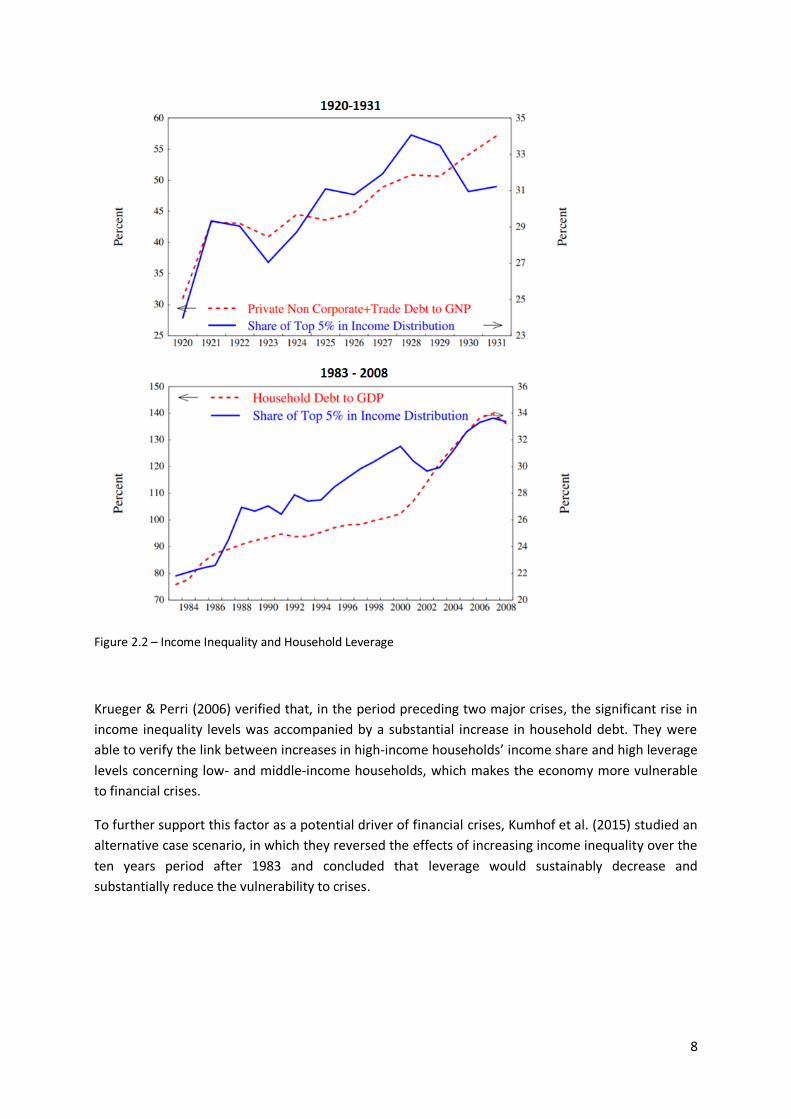
The second factor impacting credit supply is a rise in income inequality. Kumhof et al. (2015) studied

this hypothesis explaining that high-income households have a higher marginal propensity to save,

since they prefer wealth accumulation, which will act as a driver for an increase in credit supply. They

concluded that prior to both the Great Recession and the Great Depression, debt-to-income ratios

regarding both low- and middle-income households suffered a sharp increase simultaneously, being

that the savings from the high-income household segment acted as a credit supply expansion to the

former, establishing the connection between a rise in income inequality and the above-mentioned

shocks (Figure 2.2).

8

Figure 2.2 – Income Inequality and Household Leverage

Krueger & Perri (2006) verified that, in the period preceding two major crises, the significant rise in

income inequality levels was accompanied by a substantial increase in household debt. They were

able to verify the link between increases in high-income households’ income share and high leverage

levels concerning low- and middle-income households, which makes the economy more vulnerable

to financial crises.

To further support this factor as a potential driver of financial crises, Kumhof et al. (2015) studied an

alternative case scenario, in which they reversed the effects of increasing income inequality over the

ten years period after 1983 and concluded that leverage would sustainably decrease and

substantially reduce the vulnerability to crises.

9

2.1.3. Financial Liberalization and Deregulation

Finally, the third driver is related to financial liberalization and deregulation. According to Aliber &

Kindleberger (2005), this phenomenon was a driving force which led to monetary expansion, foreign

borrowing and investment speculation and affected several different countries, such as Japan,

Mexico, Russia and the Scandinavian countries.

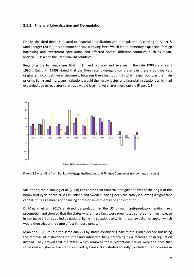
Regarding the banking crises that hit Finland, Norway and Sweden in the late 1980’s and early

1990’s, Englund (1999) stated that the then recent deregulation present in these credit markets

originated a competitive environment between these institutions in which expansion was the main

priority. Banks and mortgage institutions would then grow faster, and financial institutions which had

expanded due to regulatory arbitrage would lose market shares more rapidly (Figure 2.3).

Figure 2.3 – Lending from Banks, Mortgage Institutions, and Finance Companies (percentage changes)

Still on this topic, Jonung et al. (2008) considered that financial deregulation was at the origin of the

boom-bust cycle of the crises in Finland and Sweden, having been the catalyst allowing a significant

capital influx as a means of financing domestic investments and consumption.

Di Maggio et al. (2017) analyzed deregulation in the US through anti-predatory lending laws

preemption and showed that the states where these laws were preempted suffered from an increase

in mortgage credit supplied by national banks - institutions to which these laws did not apply - which

would then trigger the same effect in house prices.

Mian et al. (2017a) did the same analysis by states considering part of the 1980’s decade but using

the removal of restrictions on inter and intrastate bank branching as a measure of deregulation

instead. They proved that the states which removed these restrictions earlier were the ones that

witnessed a higher rise in credit supplied by banks. Both studies soundly concluded that increases in

10

credit supply directly related to banking deregulation create a larger rise in debt in the short term

and a stronger recession in the medium term.

We have now established a solid connection between credit supply expansions and financial crises -

through saving gluts, rises in income inequality and financial deregulation - taking this factor as a

major driver of the boom-bust cycle.

2.2. SECOND PILLAR: HOUSEHOLD DEBT

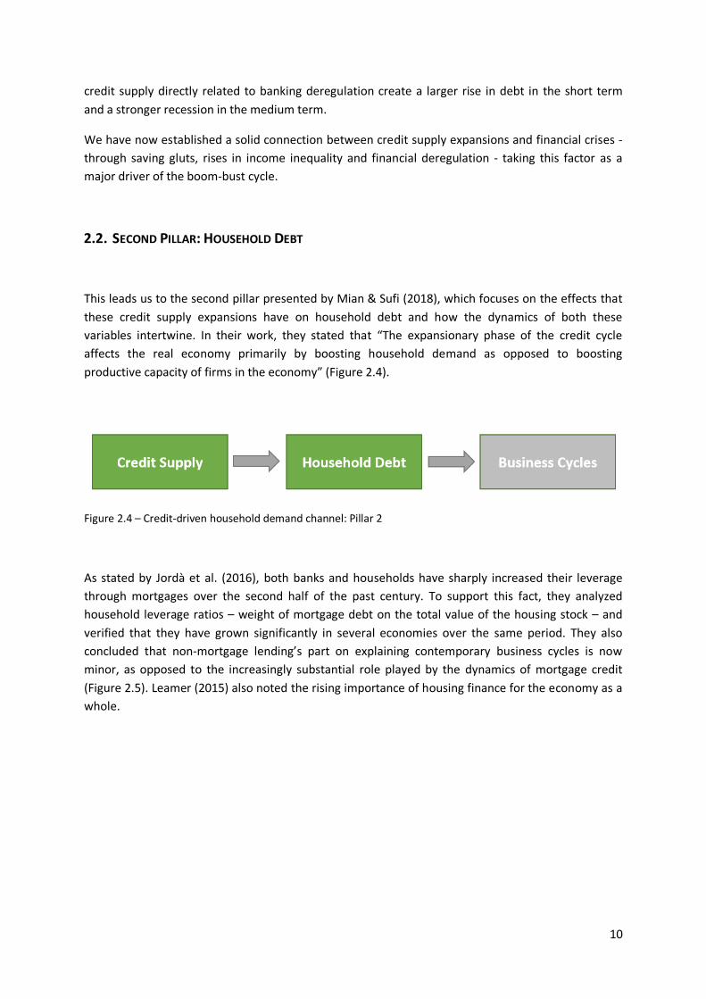
This leads us to the second pillar presented by Mian & Sufi (2018), which focuses on the effects that

these credit supply expansions have on household debt and how the dynamics of both these

variables intertwine. In their work, they stated that “The expansionary phase of the credit cycle

affects the real economy primarily by boosting household demand as opposed to boosting

productive capacity of firms in the economy” (Figure 2.4).


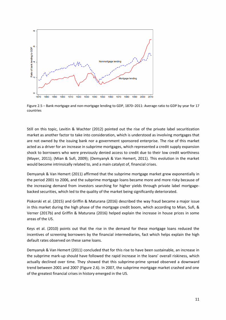
As stated by Jordà et al. (2016), both banks and households have sharply increased their leverage

through mortgages over the second half of the past century. To support this fact, they analyzed

household leverage ratios – weight of mortgage debt on the total value of the housing stock – and

verified that they have grown significantly in several economies over the same period. They also

concluded that non-mortgage lending’s part on explaining contemporary business cycles is now

minor, as opposed to the increasingly substantial role played by the dynamics of mortgage credit

(Figure 2.5). Leamer (2015) also noted the rising importance of housing finance for the economy as a

whole.

11

Figure 2.5 – Bank mortgage and non-mortgage lending to GDP, 1870–2011: Average ratio to GDP by year for 17 countries

Still on this topic, Levitin & Wachter (2012) pointed out the rise of the private label securitization

market as another factor to take into consideration, which is understood as involving mortgages that

are not owned by the issuing bank nor a government sponsored enterprise. The rise of this market

acted as a driver for an increase in subprime mortgages, which represented a credit supply expansion

shock to borrowers who were previously denied access to credit due to their low credit worthiness

(Mayer, 2011); (Mian & Sufi, 2009); (Demyanyk & Van Hemert, 2011). This evolution in the market

would become intrinsically related to, and a main catalyst of, financial crises.

Demyanyk & Van Hemert (2011) affirmed that the subprime mortgage market grew exponentially in

the period 2001 to 2006, and the subprime mortgage loans became more and more risky because of

the increasing demand from investors searching for higher yields through private label mortgage-

backed securities, which led to the quality of the market being significantly deteriorated.

Piskorski et al. (2015) and Griffin & Maturana (2016) described the way fraud became a major issue

in this market during the high phase of the mortgage credit boom, which according to Mian, Sufi, &

Verner (2017b) and Griffin & Maturana (2016) helped explain the increase in house prices in some

areas of the US.

Keys et al. (2010) points out that the rise in the demand for these mortgage loans reduced the

incentives of screening borrowers by the financial intermediaries, fact which helps explain the high

default rates observed on these same loans.

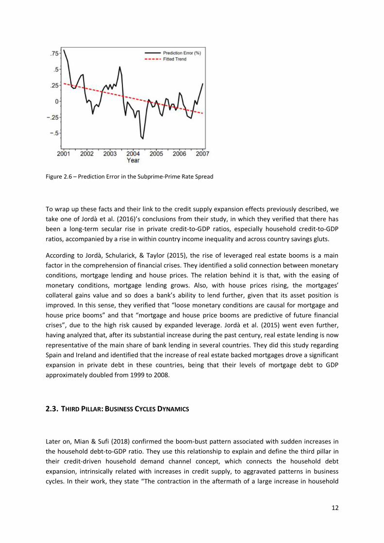
Demyanyk & Van Hemert (2011) concluded that for this rise to have been sustainable, an increase in

the subprime mark-up should have followed the rapid increase in the loans’ overall riskiness, which

actually declined over time. They showed that this subprime-prime spread observed a downward

trend between 2001 and 2007 (Figure 2.6). In 2007, the subprime mortgage market crashed and one

of the greatest financial crises in history emerged in the US.

12

Figure 2.6 – Prediction Error in the Subprime-Prime Rate Spread

To wrap up these facts and their link to the credit supply expansion effects previously described, we

take one of Jordà et al. (2016)’s conclusions from their study, in which they verified that there has

been a long-term secular rise in private credit-to-GDP ratios, especially household credit-to-GDP

ratios, accompanied by a rise in within country income inequality and across country savings gluts.

According to Jordà, Schularick, & Taylor (2015), the rise of leveraged real estate booms is a main

factor in the comprehension of financial crises. They identified a solid connection between monetary

conditions, mortgage lending and house prices. The relation behind it is that, with the easing of

monetary conditions, mortgage lending grows. Also, with house prices rising, the mortgages’

collateral gains value and so does a bank’s ability to lend further, given that its asset position is

improved. In this sense, they verified that “loose monetary conditions are causal for mortgage and

house price booms” and that “mortgage and house price booms are predictive of future financial

crises”, due to the high risk caused by expanded leverage. Jordà et al. (2015) went even further,

having analyzed that, after its substantial increase during the past century, real estate lending is now

representative of the main share of bank lending in several countries. They did this study regarding

Spain and Ireland and identified that the increase of real estate backed mortgages drove a significant

expansion in private debt in these countries, being that their levels of mortgage debt to GDP

approximately doubled from 1999 to 2008.

2.3. THIRD PILLAR: BUSINESS CYCLES DYNAMICS

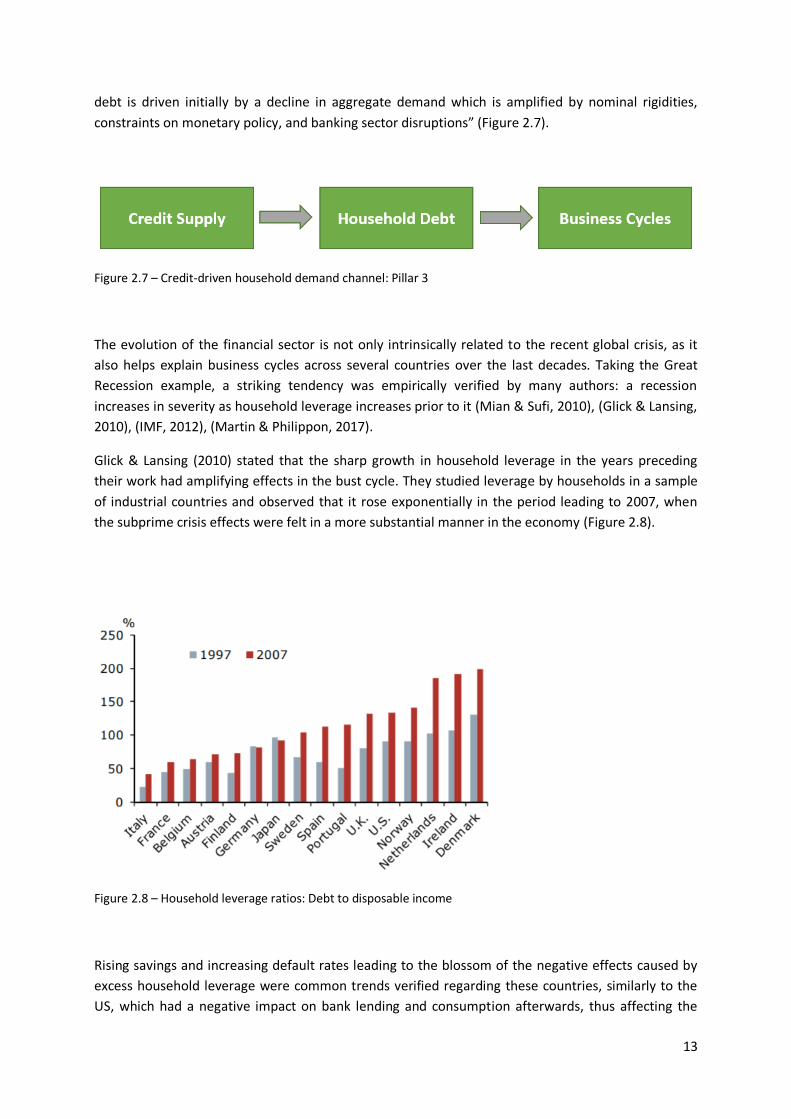
Later on, Mian & Sufi (2018) confirmed the boom-bust pattern associated with sudden increases in

the household debt-to-GDP ratio. They use this relationship to explain and define the third pillar in

their credit-driven household demand channel concept, which connects the household debt

expansion, intrinsically related with increases in credit supply, to aggravated patterns in business

cycles. In their work, they state “The contraction in the aftermath of a large increase in household

13

debt is driven initially by a decline in aggregate demand which is amplified by nominal rigidities,

constraints on monetary policy, and banking sector disruptions” (Figure 2.7).


The evolution of the financial sector is not only intrinsically related to the recent global crisis, as it

also helps explain business cycles across several countries over the last decades. Taking the Great

Recession example, a striking tendency was empirically verified by many authors: a recession

increases in severity as household leverage increases prior to it (Mian & Sufi, 2010), (Glick & Lansing,

2010), (IMF, 2012), (Martin & Philippon, 2017).

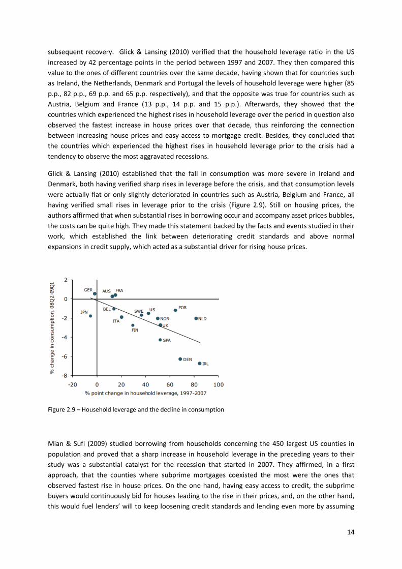
Glick & Lansing (2010) stated that the sharp growth in household leverage in the years preceding

their work had amplifying effects in the bust cycle. They studied leverage by households in a sample

of industrial countries and observed that it rose exponentially in the period leading to 2007, when

the subprime crisis effects were felt in a more substantial manner in the economy (Figure 2.8).

Figure 2.8 – Household leverage ratios: Debt to disposable income

Rising savings and increasing default rates leading to the blossom of the negative effects caused by

excess household leverage were common trends verified regarding these countries, similarly to the

US, which had a negative impact on bank lending and consumption afterwards, thus affecting the

14

subsequent recovery. Glick & Lansing (2010) verified that the household leverage ratio in the US

increased by 42 percentage points in the period between 1997 and 2007. They then compared this

value to the ones of different countries over the same decade, having shown that for countries such

as Ireland, the Netherlands, Denmark and Portugal the levels of household leverage were higher (85

p.p., 82 p.p., 69 p.p. and 65 p.p. respectively), and that the opposite was true for countries such as

Austria, Belgium and France (13 p.p., 14 p.p. and 15 p.p.). Afterwards, they showed that the

countries which experienced the highest rises in household leverage over the period in question also

observed the fastest increase in house prices over that decade, thus reinforcing the connection

between increasing house prices and easy access to mortgage credit. Besides, they concluded that

the countries which experienced the highest rises in household leverage prior to the crisis had a

tendency to observe the most aggravated recessions.

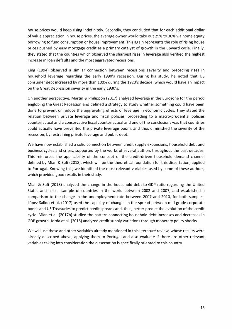
Glick & Lansing (2010) established that the fall in consumption was more severe in Ireland and

Denmark, both having verified sharp rises in leverage before the crisis, and that consumption levels

were actually flat or only slightly deteriorated in countries such as Austria, Belgium and France, all

having verified small rises in leverage prior to the crisis (Figure 2.9). Still on housing prices, the

authors affirmed that when substantial rises in borrowing occur and accompany asset prices bubbles,

the costs can be quite high. They made this statement backed by the facts and events studied in their

work, which established the link between deteriorating credit standards and above normal

expansions in credit supply, which acted as a substantial driver for rising house prices.

Figure 2.9 – Household leverage and the decline in consumption

Mian & Sufi (2009) studied borrowing from households concerning the 450 largest US counties in

population and proved that a sharp increase in household leverage in the preceding years to their

study was a substantial catalyst for the recession that started in 2007. They affirmed, in a first

approach, that the counties where subprime mortgages coexisted the most were the ones that

observed fastest rise in house prices. On the one hand, having easy access to credit, the subprime

buyers would continuously bid for houses leading to the rise in their prices, and, on the other hand,

this would fuel lenders’ will to keep loosening credit standards and lending even more by assuming

15

house prices would keep rising indefinitely. Secondly, they concluded that for each additional dollar

of value appreciation in house prices, the average owner would take out 25% to 30% via home equity

borrowing to fund consumption or house improvement. This again represents the role of rising house

prices pushed by easy mortgage credit as a primary catalyst of growth in the upward cycle. Finally,

they stated that the counties which observed the sharpest rises in leverage also verified the highest

increase in loan defaults and the most aggravated recessions.

King (1994) observed a similar connection between recessions severity and preceding rises in

household leverage regarding the early 1990’s recession. During his study, he noted that US

consumer debt increased by more than 100% during the 1920’s decade, which would have an impact

on the Great Depression severity in the early 1930’s.

On another perspective, Martin & Philippon (2017) analyzed leverage in the Eurozone for the period

englobing the Great Recession and defined a strategy to study whether something could have been

done to prevent or reduce the aggravating effects of leverage in economic cycles. They stated the

relation between private leverage and fiscal policies, proceeding to a macro-prudential policies

counterfactual and a conservative fiscal counterfactual and one of the conclusions was that countries

could actually have prevented the private leverage boom, and thus diminished the severity of the

recession, by restraining private leverage and public debt.

We have now established a solid connection between credit supply expansions, household debt and

business cycles and crises, supported by the works of several authors throughout the past decades.

This reinforces the applicability of the concept of the credit-driven household demand channel

defined by Mian & Sufi (2018), which will be the theoretical foundation for this dissertation, applied

to Portugal. Knowing this, we identified the most relevant variables used by some of these authors,

which provided good results in their study.

Mian & Sufi (2018) analyzed the change in the household debt-to-GDP ratio regarding the United

States and also a sample of countries in the world between 2002 and 2007, and established a

comparison to the change in the unemployment rate between 2007 and 2010, for both samples.

López-Salido et al. (2017) used the capacity of changes in the spread between mid-grade corporate

bonds and US Treasuries to predict credit spreads and, thus, better predict the evolution of the credit

cycle. Mian et al. (2017b) studied the pattern connecting household debt increases and decreases in

GDP growth. Jordà et al. (2015) analyzed credit supply variations through monetary policy shocks.

We will use these and other variables already mentioned in this literature review, whose results were

already described above, applying them to Portugal and also evaluate if there are other relevant

variables taking into consideration the dissertation is specifically oriented to this country.

16

3. METHODOLOGY AND RESULTS ANALYSIS

3.1. DATA SELECTION AND VARIABLES DEFINITION

Our work started with a literature review of the most relevant studies made by several authors on

this topic. We investigated how credit supply affects household debt and how this debt is related to

financial crises. Regarding the subject, we analysed the work of Mian and Sufi in “Finance and

Business Cycles: The Credit-Driven Household Demand Channel” (Mian & Sufi, 2018), which uses

statistical methods to study the effects that certain economic and financial indicators have on the

development of business cycles and establishes a connection between credit supply, household debt

and financial crises. Taking this into consideration, we used this fundamental basis concerning

household debt by applying it to Portugal in our study of the evolution of household debt and how it

is affected by a series of other variables, having selected and adapted the most relevant variables

used by these authors and applied them to reach our study objectives. Our focus will be the period

between 2003 and 2018, which is comprised of sixteen years. We will use 2018 as the cut-off year

since it is the most recent year for which there is complete data, and start sixteen years before that,

in 2003, the first full year after the removal of the “escudo” from circulation and, thus, the full usage

of the euro as the only official currency in circulation in Portugal.

In order to do this, we researched and collected data from some of the main statistical information

sources in Portugal and the world. The variables that we defined are as follows (Table 3.1):

Variables

Household debt to GDP Consumption to GDP Government debt to GDP Net exports to GDP Nominal exports Nominal imports Non-financial firm debt to GDP Real consumption Real durable consumption Real effective exchange rate Real GDP Real government consumption Real house price index Real investment Real nondurable consumption Unemployment rate

Table 3.1 – Variables

17

Most of the data that composes our variables was acquired from the databases of Banco de Portugal

(the Portuguese Central Bank) and Instituto Nacional de Estatística (INE). This includes information

concerning GDP levels, consumption, imports and exports and investment, and also more specific

data, such as mortgage and corporate spreads in relation to sovereign spreads.

The majority of debt related data, namely household debt to GDP, non-financial firm debt to GDP

and government debt to GDP was obtained from the Bank for International Settlements (BIS).

Information for more specific variables, such as the real effective exchange rate and the real house

price index was gathered in the World Bank’s database and the forecast of growth from t to t+3 was

obtained from the International Monetary Fund Fall World Economic Outlook.

After gathering all the intended data, we filtered, segregated and allocated it in order to reach the

values for our defined variables in the period of study. We then centralized all the variables and their

corresponding data for the period between 2003 and 2018 in a table, in order to build the relevant

statistics.

We selected “Household debt to GDP”, which represents the total credit to households (core debt) as

a percentage of GDP in Portugal, as the independent variable, since its behaviour is the core

component we intend to study and explain in our work. The remaining variables were used to explain

the abovementioned behaviour, through their relations with “Household debt to GDP”, and the most

relevant ones were also be target of individual analysis.

3.2. DESCRIPTIVE STATISTICS

After collecting all of the data, we built the descriptive statistics for each individual variable using the

"Data Analysis" tool in Excel (Table 3.2): the variables which represent measures relative to the GDP,

as well as “Unemployment rate” and “Real effective exchange rate”, should be read in percentage

units; “Real house price index” should be interpreted as an index; the remaining variables are

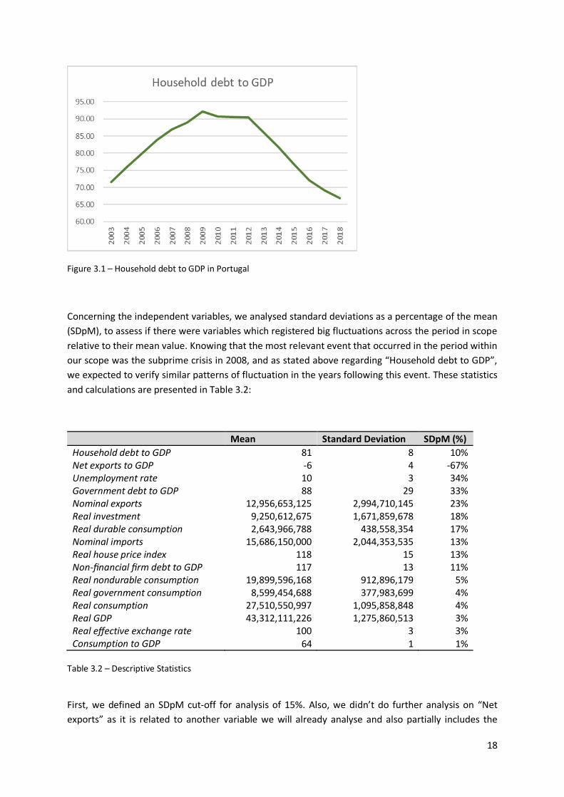
represented in Euros. From the calculated statistics, we focused in the "Mean" and "Standard

deviation". Regarding "Household debt to GDP", we noted that it comprises a mean of 81% and

standard deviation of 8%, which is related to the fact that this indicator had been increasing since

2003 until 2009, one year after the subprime financial crisis hit the US markets, remaining with

values of approximately 90% until 2012, the year when it progressively started to decrease as shown

in Figure 3.1.

18

Figure 3.1 – Household debt to GDP in Portugal

Concerning the independent variables, we analysed standard deviations as a percentage of the mean

(SDpM), to assess if there were variables which registered big fluctuations across the period in scope

relative to their mean value. Knowing that the most relevant event that occurred in the period within

our scope was the subprime crisis in 2008, and as stated above regarding “Household debt to GDP”,

we expected to verify similar patterns of fluctuation in the years following this event. These statistics

and calculations are presented in Table 3.2:

Mean Standard Deviation SDpM (%)

Household debt to GDP 81 8 10% Net exports to GDP -6 4 -67% Unemployment rate 10 3 34% Government debt to GDP 88 29 33% Nominal exports 12,956,653,125 2,994,710,145 23% Real investment 9,250,612,675 1,671,859,678 18% Real durable consumption 2,643,966,788 438,558,354 17% Nominal imports 15,686,150,000 2,044,353,535 13% Real house price index 118 15 13% Non-financial firm debt to GDP 117 13 11% Real nondurable consumption 19,899,596,168 912,896,179 5% Real government consumption 8,599,454,688 377,983,699 4% Real consumption 27,510,550,997 1,095,858,848 4% Real GDP 43,312,111,226 1,275,860,513 3% Real effective exchange rate 100 3 3% Consumption to GDP 64 1 1%

Table 3.2 – Descriptive Statistics

First, we defined an SDpM cut-off for analysis of 15%. Also, we didn’t do further analysis on “Net

exports” as it is related to another variable we will already analyse and also partially includes the

19

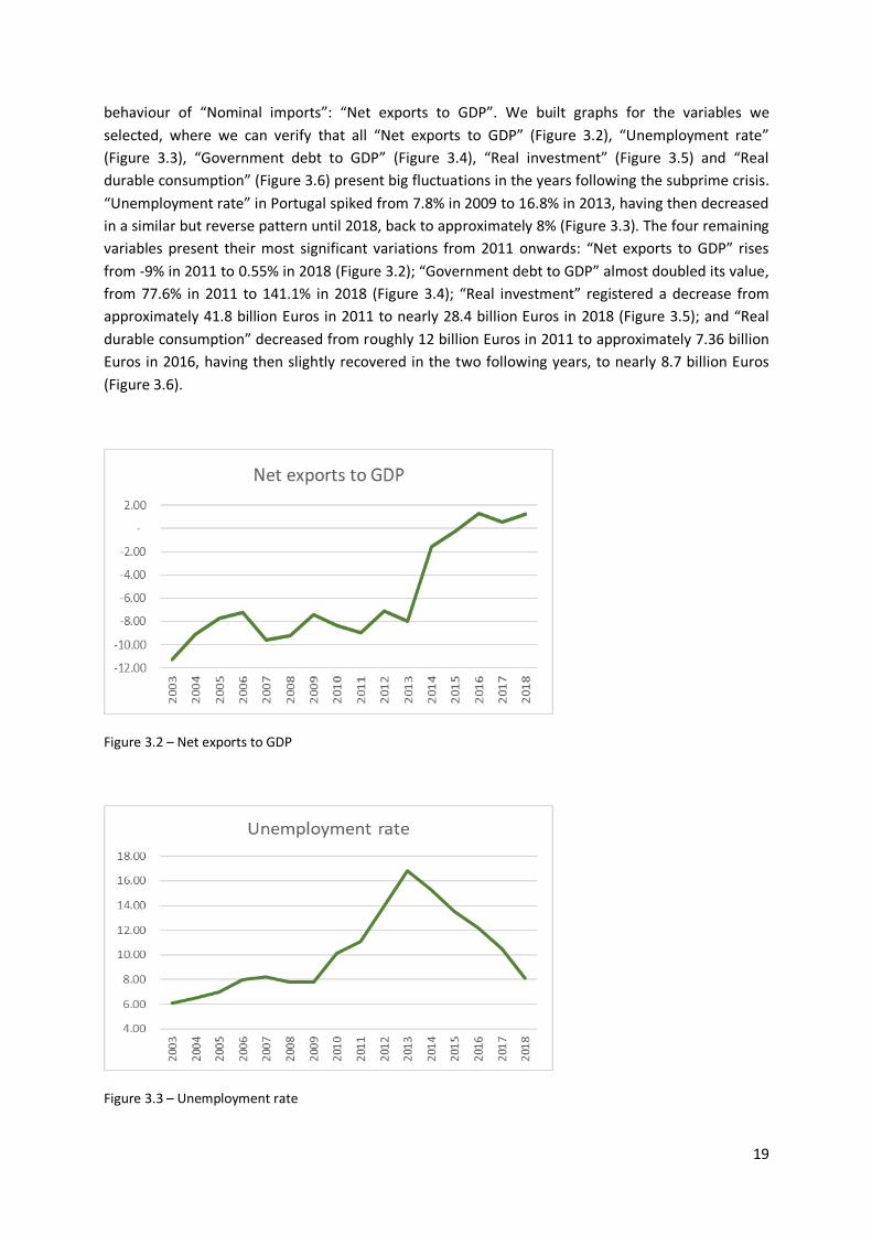
behaviour of “Nominal imports”: “Net exports to GDP”. We built graphs for the variables we

selected, where we can verify that all “Net exports to GDP” (Figure 3.2), “Unemployment rate”

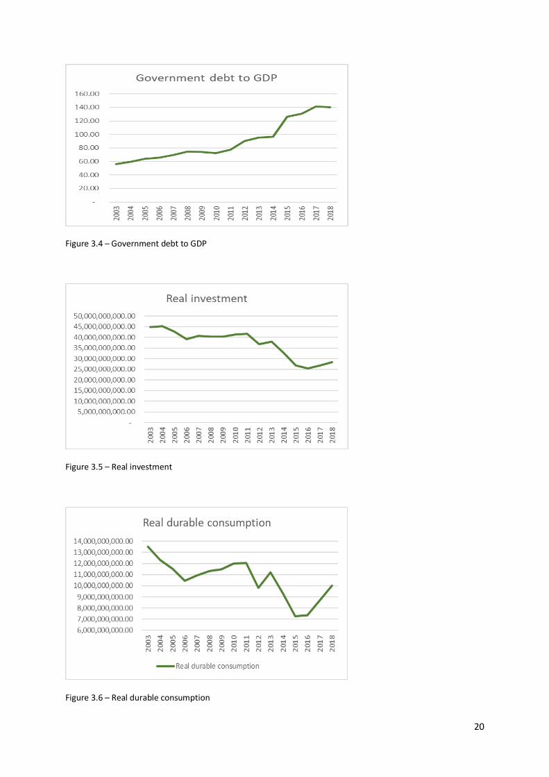
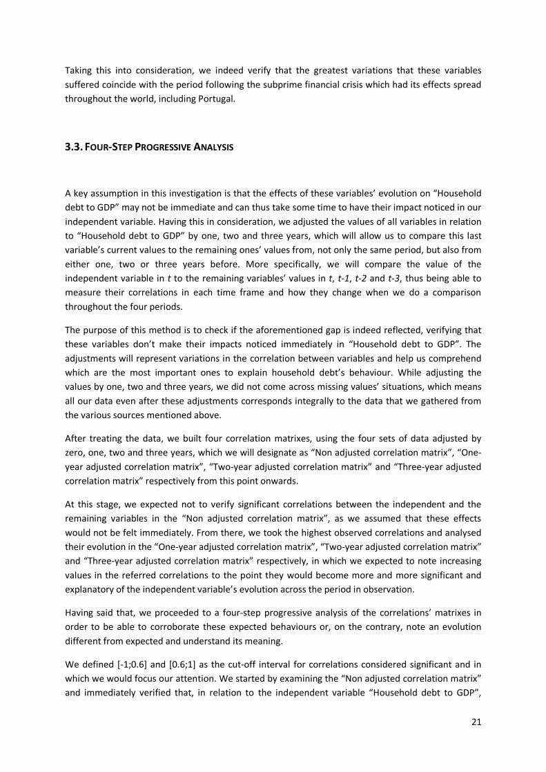
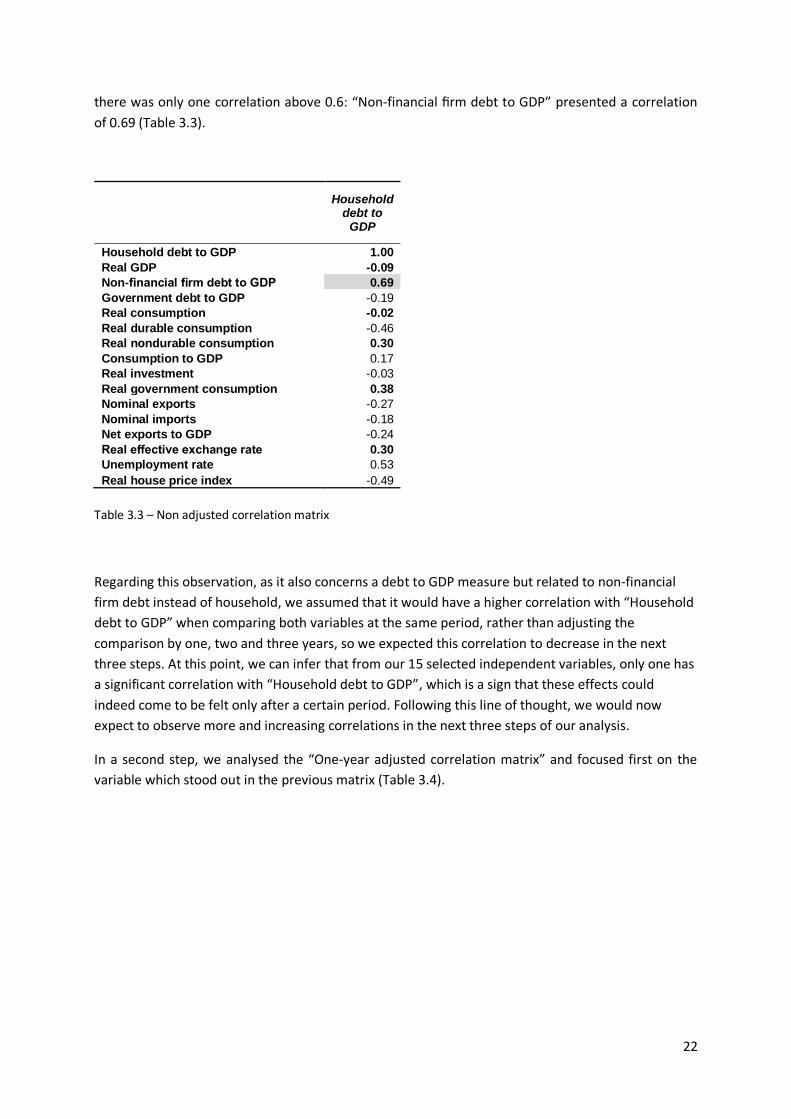
(Figure 3.3), “Government debt to GDP” (Figure 3.4), “Real investment” (Figure 3.5) and “Real

durable consumption” (Figure 3.6) present big fluctuations in the years following the subprime crisis.

“Unemployment rate” in Portugal spiked from 7.8% in 2009 to 16.8% in 2013, having then decreased

in a similar but reverse pattern until 2018, back to approximately 8% (Figure 3.3). The four remaining

variables present their most significant variations from 2011 onwards: “Net exports to GDP” rises

from -9% in 2011 to 0.55% in 2018 (Figure 3.2); “Government debt to GDP” almost doubled its value,

from 77.6% in 2011 to 141.1% in 2018 (Figure 3.4); “Real investment” registered a decrease from

approximately 41.8 billion Euros in 2011 to nearly 28.4 billion Euros in 2018 (Figure 3.5); and “Real

durable consumption” decreased from roughly 12 billion Euros in 2011 to approximately 7.36 billion

Euros in 2016, having then slightly recovered in the two following years, to nearly 8.7 billion Euros

(Figure 3.6).

Figure 3.2 – Net exports to GDP

Figure 3.3 – Unemployment rate

20

Figure 3.4 – Government debt to GDP

Figure 3.5 – Real investment

Figure 3.6 – Real durable consumption

21

Taking this into consideration, we indeed verify that the greatest variations that these variables

suffered coincide with the period following the subprime financial crisis which had its effects spread

throughout the world, including Portugal.

3.3. FOUR-STEP PROGRESSIVE ANALYSIS

A key assumption in this investigation is that the effects of these variables’ evolution on “Household

debt to GDP” may not be immediate and can thus take some time to have their impact noticed in our

independent variable. Having this in consideration, we adjusted the values of all variables in relation

to “Household debt to GDP” by one, two and three years, which will allow us to compare this last

variable’s current values to the remaining ones’ values from, not only the same period, but also from

either one, two or three years before. More specifically, we will compare the value of the

independent variable in t to the remaining variables’ values in t, t-1, t-2 and t-3, thus being able to

measure their correlations in each time frame and how they change when we do a comparison

throughout the four periods.

The purpose of this method is to check if the aforementioned gap is indeed reflected, verifying that

these variables don’t make their impacts noticed immediately in “Household debt to GDP”. The

adjustments will represent variations in the correlation between variables and help us comprehend

which are the most important ones to explain household debt’s behaviour. While adjusting the

values by one, two and three years, we did not come across missing values’ situations, which means

all our data even after these adjustments corresponds integrally to the data that we gathered from

the various sources mentioned above.

After treating the data, we built four correlation matrixes, using the four sets of data adjusted by

zero, one, two and three years, which we will designate as “Non adjusted correlation matrix”, “One-

year adjusted correlation matrix”, “Two-year adjusted correlation matrix” and “Three-year adjusted

correlation matrix” respectively from this point onwards.

At this stage, we expected not to verify significant correlations between the independent and the

remaining variables in the “Non adjusted correlation matrix”, as we assumed that these effects

would not be felt immediately. From there, we took the highest observed correlations and analysed

their evolution in the “One-year adjusted correlation matrix”, “Two-year adjusted correlation matrix”

and “Three-year adjusted correlation matrix” respectively, in which we expected to note increasing

values in the referred correlations to the point they would become more and more significant and

explanatory of the independent variable’s evolution across the period in observation.

Having said that, we proceeded to a four-step progressive analysis of the correlations’ matrixes in

order to be able to corroborate these expected behaviours or, on the contrary, note an evolution

different from expected and understand its meaning.

We defined [-1;0.6] and [0.6;1] as the cut-off interval for correlations considered significant and in

which we would focus our attention. We started by examining the “Non adjusted correlation matrix”

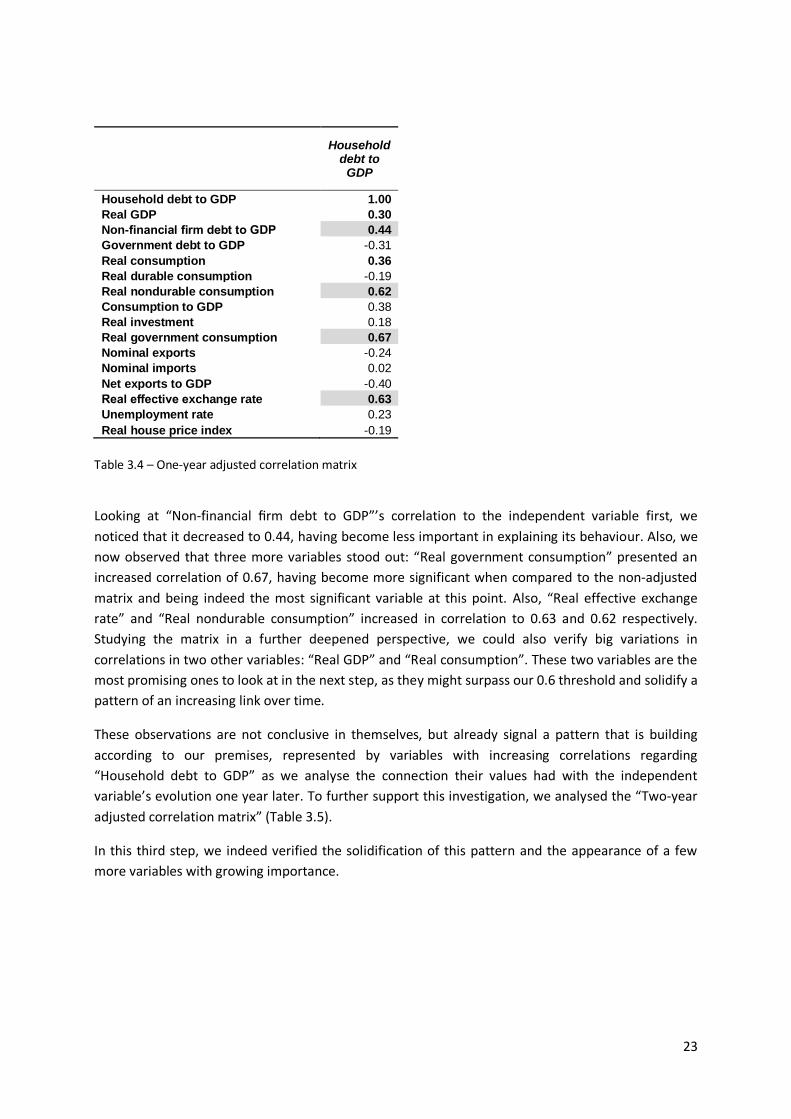
and immediately verified that, in relation to the independent variable “Household debt to GDP”,

22

there was only one correlation above 0.6: “Non-financial firm debt to GDP” presented a correlation

of 0.69 (Table 3.3).

Household debt to

GDP

Household debt to GDP 1.00

Real GDP -0.09

Non-financial firm debt to GDP 0.69

Government debt to GDP -0.19

Real consumption -0.02

Real durable consumption -0.46

Real nondurable consumption 0.30

Consumption to GDP 0.17

Real investment -0.03

Real government consumption 0.38

Nominal exports -0.27

Nominal imports -0.18

Net exports to GDP -0.24

Real effective exchange rate 0.30

Unemployment rate 0.53

Real house price index -0.49

Table 3.3 – Non adjusted correlation matrix

Regarding this observation, as it also concerns a debt to GDP measure but related to non-financial

firm debt instead of household, we assumed that it would have a higher correlation with “Household

debt to GDP” when comparing both variables at the same period, rather than adjusting the

comparison by one, two and three years, so we expected this correlation to decrease in the next

three steps. At this point, we can infer that from our 15 selected independent variables, only one has

a significant correlation with “Household debt to GDP”, which is a sign that these effects could

indeed come to be felt only after a certain period. Following this line of thought, we would now

expect to observe more and increasing correlations in the next three steps of our analysis.

In a second step, we analysed the “One-year adjusted correlation matrix” and focused first on the

variable which stood out in the previous matrix (Table 3.4).

23

Household debt to

GDP


Real GDP 0.30



Real consumption 0.36

Real durable consumption -0.19



Real investment 0.18



Nominal imports 0.02



Unemployment rate 0.23

Real house price index -0.19

Table 3.4 – One-year adjusted correlation matrix

Looking at “Non-financial firm debt to GDP”’s correlation to the independent variable first, we

noticed that it decreased to 0.44, having become less important in explaining its behaviour. Also, we

now observed that three more variables stood out: “Real government consumption” presented an

increased correlation of 0.67, having become more significant when compared to the non-adjusted

matrix and being indeed the most significant variable at this point. Also, “Real effective exchange

rate” and “Real nondurable consumption” increased in correlation to 0.63 and 0.62 respectively.

Studying the matrix in a further deepened perspective, we could also verify big variations in

correlations in two other variables: “Real GDP” and “Real consumption”. These two variables are the

most promising ones to look at in the next step, as they might surpass our 0.6 threshold and solidify a

pattern of an increasing link over time.

These observations are not conclusive in themselves, but already signal a pattern that is building

according to our premises, represented by variables with increasing correlations regarding

“Household debt to GDP” as we analyse the connection their values had with the independent

variable’s evolution one year later. To further support this investigation, we analysed the “Two-year

adjusted correlation matrix” (Table 3.5).

In this third step, we indeed verified the solidification of this pattern and the appearance of a few

more variables with growing importance.

24

Household debt to

GDP


Real GDP 0.65




Real durable consumption 0.09









Unemployment rate -0.02

Real house price index 0.04

Table 3.5 – Two-year adjusted correlation matrix

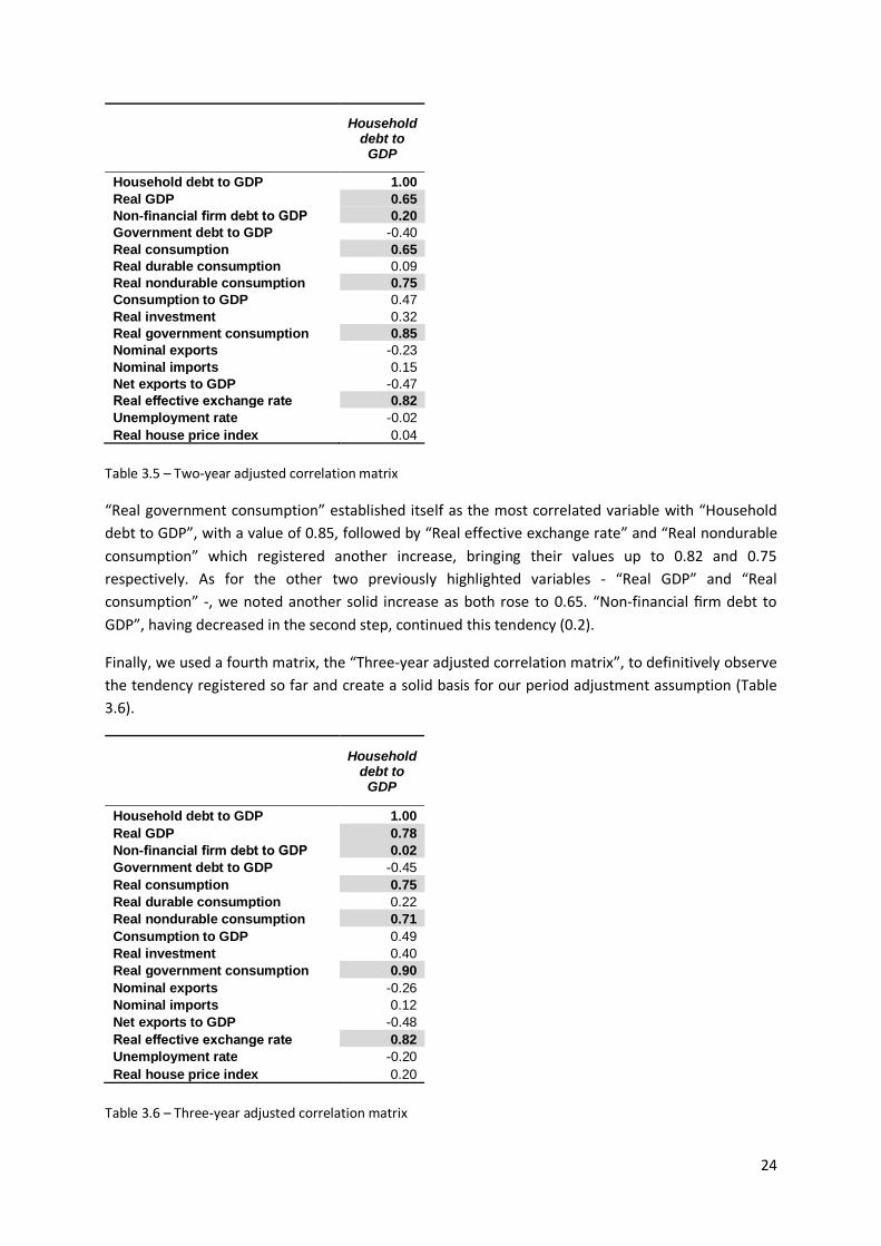
“Real government consumption” established itself as the most correlated variable with “Household

debt to GDP”, with a value of 0.85, followed by “Real effective exchange rate” and “Real nondurable

consumption” which registered another increase, bringing their values up to 0.82 and 0.75

respectively. As for the other two previously highlighted variables - “Real GDP” and “Real

consumption” -, we noted another solid increase as both rose to 0.65. “Non-financial firm debt to

GDP”, having decreased in the second step, continued this tendency (0.2).

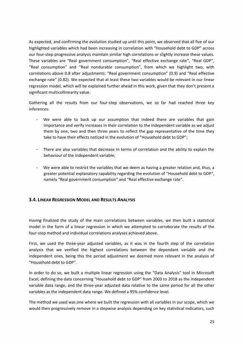
Finally, we used a fourth matrix, the “Three-year adjusted correlation matrix”, to definitively observe

the tendency registered so far and create a solid basis for our period adjustment assumption (Table

3.6).

Household debt to

GDP


Real GDP 0.78




Real durable consumption 0.22









Unemployment rate -0.20

Real house price index 0.20

Table 3.6 – Three-year adjusted correlation matrix

25

As expected, and confirming the evolution studied up until this point, we observed that all five of our

highlighted variables which had been increasing in correlation with “Household debt to GDP” across

our four-step progressive analysis maintain similar high correlations or slightly increase these values.

These variables are “Real government consumption”, “Real effective exchange rate”, “Real GDP”,

“Real consumption” and “Real nondurable consumption”, from which we highlight two, with

correlations above 0.8 after adjustments: “Real government consumption” (0.9) and “Real effective

exchange rate” (0.82). We expected that at least these two variables would be relevant in our linear

regression model, which will be explained further ahead in this work, given that they don’t present a

significant multicollinearity value.

Gathering all the results from our four-step observations, we so far had reached three key

inferences:

- We were able to back up our assumption that indeed there are variables that gain

importance and verify increases in their correlation to the independent variable as we adjust

them by one, two and then three years to reflect the gap representative of the time they

take to have their effects noticed in the evolution of “Household debt to GDP”;

- There are also variables that decrease in terms of correlation and the ability to explain the

behaviour of the independent variable;

- We were able to restrict the variables that we deem as having a greater relation and, thus, a

greater potential explanatory capability regarding the evolution of “Household debt to GDP”,

namely “Real government consumption” and “Real effective exchange rate”.

3.4. LINEAR REGRESSION MODEL AND RESULTS ANALYSIS

Having finalized the study of the main correlations between variables, we then built a statistical

model in the form of a linear regression in which we attempted to corroborate the results of the

four-step method and individual correlations analyses achieved above.

First, we used the three-year adjusted variables, as it was in the fourth step of the correlation

analysis that we verified the highest correlations between the dependant variable and the

independent ones, being this the period adjustment we deemed more relevant in the analysis of

“Household debt to GDP”.

In order to do so, we built a multiple linear regression using the “Data Analysis” tool in Microsoft

Excel, defining the data concerning “Household debt to GDP” from 2003 to 2018 as the independent

variable data range, and the three-year adjusted data relative to the same period for all the other

variables as the independent data range. We defined a 95% confidence level.

The method we used was one where we built the regression with all variables in our scope, which we

would then progressively remove in a stepwise analysis depending on key statistical indicators, such

26

as the Variance Inflator Factor (VIF) and the p-value regarding the individual variables, and the

Adjusted R Squared and F-stat regarding the overall model. The Adjusted R Squared is an indicator

which evaluates the strength of the relationship between the model and the dependent variable on a

0 to 100% range, adjusted for the number of predictors in the model. The closer to 100% its value is,

the better our model performs. Also, Akossou & Palm (2013) concluded in their study through a

Monte Carlo simulation that, while the R Squared measure is biased in linear multiple regressions,

the Adjusted R Squared is unbiased, or at least its bias is negligible.

The p-value ranges from 0 to 1 and we used it to establish a significance threshold for each of the

independent variables, through which we would reject the null hypothesis (Hassan, 2001). We

considered variables with p-value lower than 0.05 as statistically significant to our model in rejecting

the null hypothesis.

Also, we proceeded to an analysis of these p-values combined with the F-stat, in which the value of

zero represents the null hypothesis. The F-stat measures the joint significance of the variables under

study, but not their significance individually (Blackwell, 2008). This combination allows us to assess

the individual significance of each variable, without neglecting their joint significance. If low p-values

and a high F-stat value are observed simultaneously, we verify that the model has a good explanatory

capability regarding the dependent variable.

Since our model consists of a multiple linear regression, we ultimately used the Adjusted R Squared

and the ANOVA's F-stat, combined with the individual p-values, to evaluate its performance.

In a first step, we built the linear regression with all the 15 variables in our scope as independent

variables, using their three-year adjusted data, and “Household debt to GDP” as the dependent

variable.

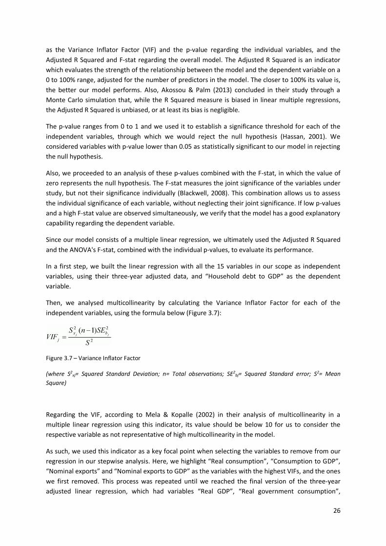
Then, we analysed multicollinearity by calculating the Variance Inflator Factor for each of the

independent variables, using the formula below (Figure 3.7):

Figure 3.7 – Variance Inflator Factor

(where S2xj= Squared Standard Deviation; n= Total observations; SE2

bj= Squared Standard error; S2= Mean

Square)

Regarding the VIF, according to Mela & Kopalle (2002) in their analysis of multicollinearity in a

multiple linear regression using this indicator, its value should be below 10 for us to consider the

respective variable as not representative of high multicollinearity in the model.

As such, we used this indicator as a key focal point when selecting the variables to remove from our

regression in our stepwise analysis. Here, we highlight “Real consumption”, “Consumption to GDP”,

“Nominal exports” and “Nominal exports to GDP” as the variables with the highest VIFs, and the ones

we first removed. This process was repeated until we reached the final version of the three-year

adjusted linear regression, which had variables “Real GDP”, “Real government consumption”,

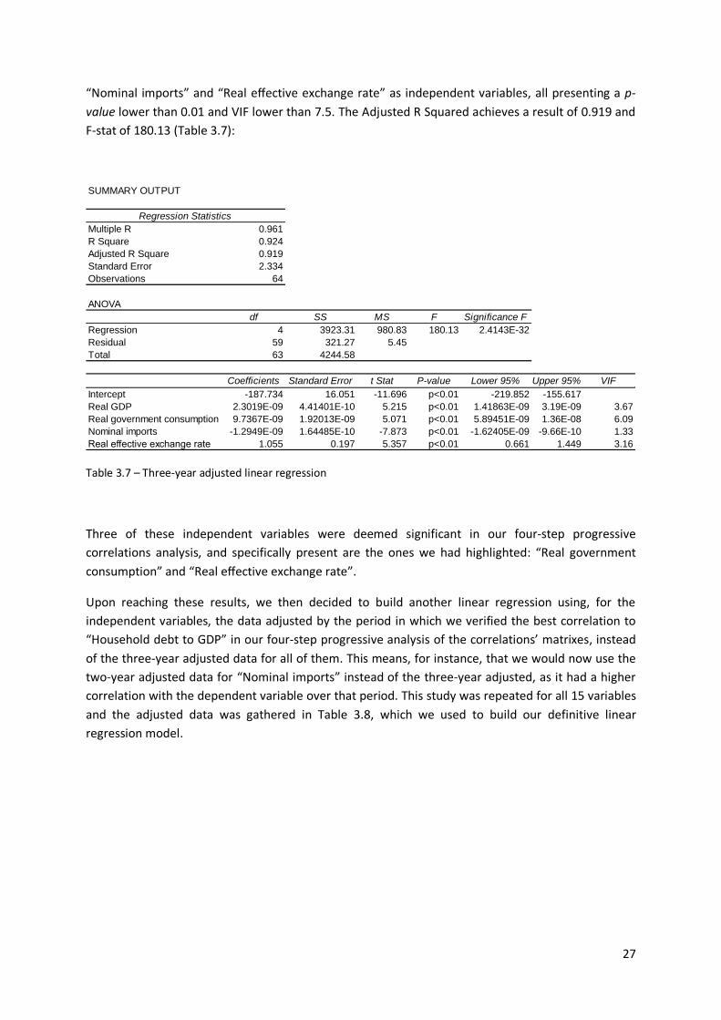
27

“Nominal imports” and “Real effective exchange rate” as independent variables, all presenting a p-

value lower than 0.01 and VIF lower than 7.5. The Adjusted R Squared achieves a result of 0.919 and

F-stat of 180.13 (Table 3.7):

SUMMARY OUTPUT

Regression Statistics

Multiple R 0.961

R Square 0.924

Adjusted R Square 0.919

Standard Error 2.334

Observations 64

ANOVA

df SS MS F Significance F

Regression 4 3923.31 980.83 180.13 2.4143E-32

Residual 59 321.27 5.45

Total 63 4244.58

Coefficients Standard Error t Stat P-value Lower 95% Upper 95% VIF

Intercept -187.734 16.051 -11.696 p<0.01 -219.852 -155.617

Real GDP 2.3019E-09 4.41401E-10 5.215 p<0.01 1.41863E-09 3.19E-09 3.67

Real government consumption 9.7367E-09 1.92013E-09 5.071 p<0.01 5.89451E-09 1.36E-08 6.09

Nominal imports -1.2949E-09 1.64485E-10 -7.873 p<0.01 -1.62405E-09 -9.66E-10 1.33

Real effective exchange rate 1.055 0.197 5.357 p<0.01 0.661 1.449 3.16

Table 3.7 – Three-year adjusted linear regression

Three of these independent variables were deemed significant in our four-step progressive

correlations analysis, and specifically present are the ones we had highlighted: “Real government

consumption” and “Real effective exchange rate”.

Upon reaching these results, we then decided to build another linear regression using, for the

independent variables, the data adjusted by the period in which we verified the best correlation to

“Household debt to GDP” in our four-step progressive analysis of the correlations’ matrixes, instead

of the three-year adjusted data for all of them. This means, for instance, that we would now use the

two-year adjusted data for “Nominal imports” instead of the three-year adjusted, as it had a higher

correlation with the dependent variable over that period. This study was repeated for all 15 variables

and the adjusted data was gathered in Table 3.8, which we used to build our definitive linear

regression model.

28

Variable Adjustment period

Real durable consumption 3

Real effective exchange rate 3

Real government consumption 3

Nominal imports 2

Non-financial firm debt to GDP 1

Consumption to GDP 3

Government debt to GDP 3

Net exports to GDP 3

Nominal exports 3

Real consumption 3

Real GDP 3

Real house price index 3

Real investment 3

Real nondurable consumption 2

Unemployment rate 1

Table 3.8 – Best correlations variables selection

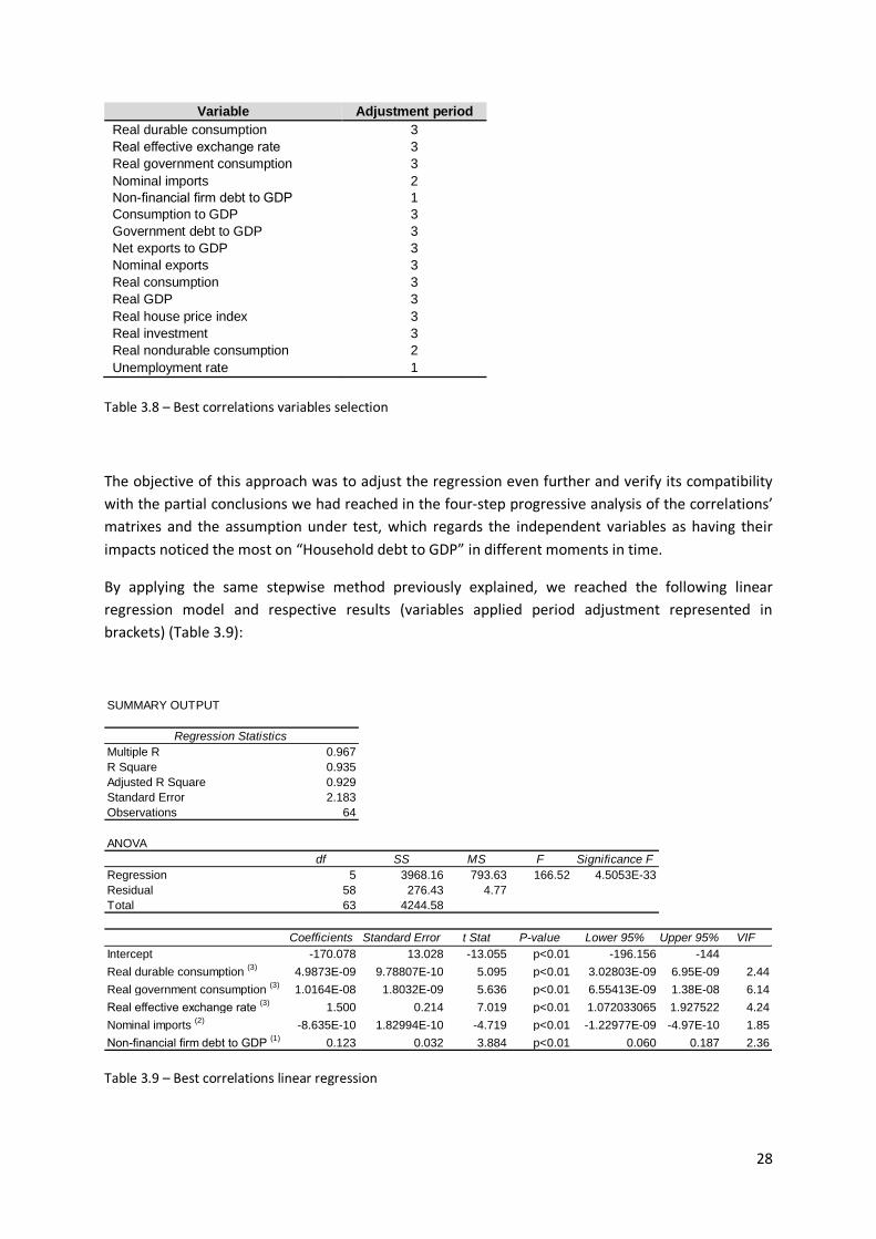
The objective of this approach was to adjust the regression even further and verify its compatibility

with the partial conclusions we had reached in the four-step progressive analysis of the correlations’

matrixes and the assumption under test, which regards the independent variables as having their

impacts noticed the most on “Household debt to GDP” in different moments in time.

By applying the same stepwise method previously explained, we reached the following linear

regression model and respective results (variables applied period adjustment represented in

brackets) (Table 3.9):

SUMMARY OUTPUT

Regression Statistics

Multiple R 0.967

R Square 0.935

Adjusted R Square 0.929

Standard Error 2.183

Observations 64

ANOVA

df SS MS F Significance F

Regression 5 3968.16 793.63 166.52 4.5053E-33

Residual 58 276.43 4.77

Total 63 4244.58

Coefficients Standard Error t Stat P-value Lower 95% Upper 95% VIF

Intercept -170.078 13.028 -13.055 p<0.01 -196.156 -144

Real durable consumption (3)

4.9873E-09 9.78807E-10 5.095 p<0.01 3.02803E-09 6.95E-09 2.44

Real government consumption (3)

1.0164E-08 1.8032E-09 5.636 p<0.01 6.55413E-09 1.38E-08 6.14

Real effective exchange rate (3)

1.500 0.214 7.019 p<0.01 1.072033065 1.927522 4.24

Nominal imports (2)

-8.635E-10 1.82994E-10 -4.719 p<0.01 -1.22977E-09 -4.97E-10 1.85

Non-financial firm debt to GDP (1)

0.123 0.032 3.884 p<0.01 0.060 0.187 2.36

Table 3.9 – Best correlations linear regression

29

As in the previous three-year adjusted linear regression model, variables “Real government

consumption”, “Nominal imports” and “Real effective exchange rate” were selected as independent

variables, but “Real GDP” was not deemed as one of the best variables to improve our model.

Besides, two new variables were selected during the process: “Real durable consumption” and “Non-

financial firm debt to GDP”. This shows that, by considering the best correlations across a three-year

period adjustment with “Household debt to GDP”, the variables selected in the stepwise method

were different than the ones we got by considering simply the three-year adjusted variables across

the scope.

All the selected variables present a p-value lower than 0.01, which is indicative of high significance,

and VIFs lower than the 7.5 threshold defined for our study. The regression returns an improved

Adjusted R Squared of 0.929 relative to the previous model, while maintaining a highly significant

value of 166.52, regarding the F-stat. It’s also worth noting that, analysing the coefficients, the

variables whose variations translated into the highest coefficients relative to the dependent variable

were “Real effective exchange rate” and “Non-financial firm debt to GDP”. The variations of the

remaining three, i.e. “Real government consumption”, “Real durable consumption” and “Nominal

imports” registered lower coefficients but are nevertheless highly significant explanatory variables

according to the model’s results. The importance of the lower coefficients achieved for these three

variables will be studied further below.

The model’s results indicate that the fact that we considered the best correlations between the

independent variables and the dependent variable “Household debt to GDP” improved the

performance of the model, and further solidifies the assumption that the effects of variations in

these variables are the most impactful in different moments in time.

In sum, in our definitive linear regression model, the behaviour of “Household debt to GDP” is best

explained by the values of “Real durable consumption”, “Real effective exchange rate” and “Real

government consumption” from three years prior, “Nominal Imports” from two years prior and

“Non-financial firm debt to GDP” from the previous year.

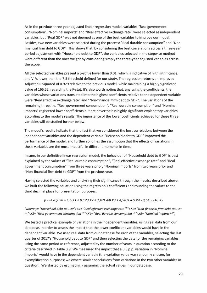
Having selected the variables and analysing their significance through the metrics described above,

we built the following equation using the regression’s coefficients and rounding the values to the

third decimal place for presentation purposes:

y = -170,078 + 1,5 X1 + 0,123 X2 + 1,02E-08 X3 + 4,987E-09 X4 - 8,645E-10 X5

(where y= “Household debt to GDP”; X1= “Real effective exchange rate (3)”; X2= “Non-financial firm debt to GDP (1)”; X3= “Real government consumption (3)”; X4= “Real durable consumption (3)”; X5= “Nominal imports (2)”)

We tested a practical example of variations in the independent variables, using real data from our

database, in order to assess the impact that the lower coefficient variables would have in the

dependent variable. We used real data from our database for each of the variables, selecting the last

quarter of 2017’s “Household debt to GDP” and then selecting the data for the remaining variables

using the same period as reference, adjusted by the number of years in question according to the

criteria described in Table 3.9. We measured the impact that a 0.3 p.p. variation in “Nominal

imports” would have in the dependent variable (the variation value was randomly chosen, for

exemplification purposes; we expect similar conclusions from variations in the two other variables in

question). We started by estimating y assuming the actual values in our database:

30

y 31/12/2017 = -170.078 + 1.5 (98.6) + 0.123 (111.7) + 1.02E-08 (8,291,318,000) + 4.987E-09

(2,305,713,839) - 8,645E-10 (17,747,400,000) = 72.00

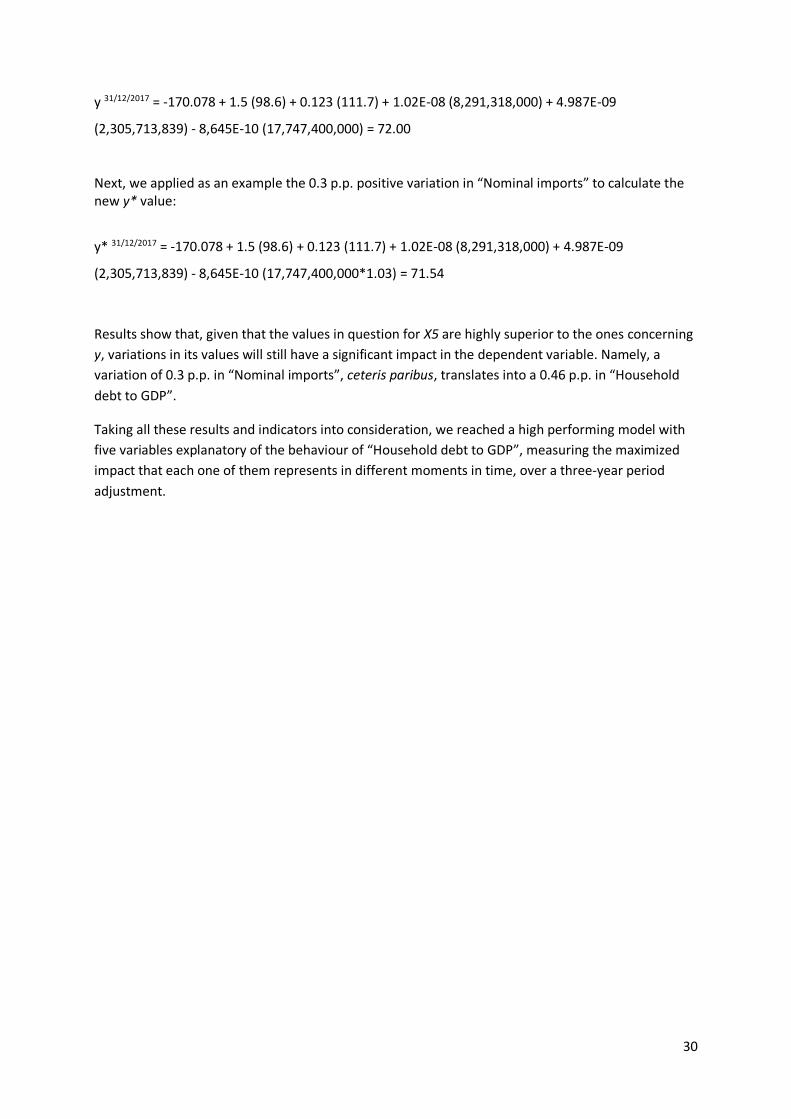
Next, we applied as an example the 0.3 p.p. positive variation in “Nominal imports” to calculate the new y* value:

y* 31/12/2017 = -170.078 + 1.5 (98.6) + 0.123 (111.7) + 1.02E-08 (8,291,318,000) + 4.987E-09

(2,305,713,839) - 8,645E-10 (17,747,400,000*1.03) = 71.54

Results show that, given that the values in question for X5 are highly superior to the ones concerning

y, variations in its values will still have a significant impact in the dependent variable. Namely, a

variation of 0.3 p.p. in “Nominal imports”, ceteris paribus, translates into a 0.46 p.p. in “Household

debt to GDP”.

Taking all these results and indicators into consideration, we reached a high performing model with

five variables explanatory of the behaviour of “Household debt to GDP”, measuring the maximized

impact that each one of them represents in different moments in time, over a three-year period

adjustment.

31

4. CONCLUSIONS AND FUTURE INVESTIGATION

After its progressive increase until 2009, household debt to GDP in Portugal has been consistently

decreasing since then until 2018, from 92% to 69% (Figure 3.1). This behaviour is similar to the ones

of several other countries around the world (Alter, Xiaochen Feng, & Valckx, 2018), which has the

subprime crisis originated in the U.S. as a main turning point.

We concluded that, regarding the Portuguese case, this indicator is explained by the evolution of

other variables, which have their impacts maximized on household debt to GDP in different moments

in time. Real durable consumption, the real effective exchange rate and real government

consumption from three years prior, nominal imports from two years prior and non-financial firm

debt to GDP from the previous year are the indicators that better explain its behaviour in the current

period of analysis.

In fact, restrictions applied to credit concession and the reinforcement of international banking

regulations via the Basel agreements and other regulatory frameworks applied following the

abovementioned crisis were essential for controlling and reducing overall indebtedness across the

economies and guaranteeing financial stability. The progressive reduction in real government

consumption and non-financial firm debt to GDP after these events is then an understandable

behaviour and explanatory of the subsequent decrease in household debt to GDP, as is the decrease

in real durable consumption after such constraints were put in place (Annex 6.1) (Annex 6.2) (Figure

1) (Figure 5). An overall more stable pattern verified in both banks and households balance sheets

was essential in the evolution that these indicators presented over the past decade. Still on the topic,

we verified that Portugal’s nominal imports observed a sharp decrease in 2010, and then resumed

their growth in a decelerated manner. From 2010 to 2018, nominal imports verified a 0,5 billion

euros reduction, which compared to the 22 billion euros increase in the previous eight years and the

fact that nominal exports kept a consistent growth pattern signals that there was also a change in the

Portuguese external commercial strategy which contributed to the change in the household debt to

GDP paradigm (Annex 6.3) (Annex 6.4) (Figure 1). The real effective exchange rate, being analysed in

this work after the implementation of the Euro in Portugal, consistently decreased after stopping its

sharp growth and thus stabilizing in 2006, fact that further corroborates our analysis regarding a

trade strategy which favours exports in detriment of growth in imports (Annex 6.5).

These are the main factors which, in different moments in time, explain the behaviour of household

debt to GDP in Portugal, which was rising until the subprime financial crisis hit the markets and then

inverted this tendency after it and the implementation of a stricter regulatory framework, as

happened in other countries. By considering the period in which the independent variables were best

correlated with household debt to GDP across a three-year period adjustment, we reached a model

with improved performance. This reinforces our initial assumption that by adjusting these indicators

period of analysis we could reach the conclusion that their effects in the variable at study are not

immediate nor linear among our scope.

Having this in consideration, this work provides some interesting possibilities for future studies. First,

an analysis of the main variables impacting household debt to GDP in other countries across Europe

and the globe would be a promising basis for studying how different countries macroeconomic and

financial strategies, political conditions and other factors contribute to observing different variables

32

affecting this indicator. A second promising study would be analysing if the fact that different

variables affect Portuguese household debt to GDP in different moments in time is a pattern that is

also observed in other countries, and if this same pattern has a different period adjustment

structure. Finally, this study uses the fundamental basis verified by Mian and Sufi (2018) and

solidified by Alter, Xiaochen Feng, & Valckx (2018) in their IMF published paper that there is a

connection between credit supply, household debt and financial business cycles and focuses in

explaining the factors that contribute to explaining the second. Applying the same analysis to credit

supply would further improve the fundaments of this cycle and help identify patterns which

contribute to explaining the behaviour of its first indicator.

In a definitive perspective, applying predictive statistics techniques complemented by fundamental

macroeconomic analysis to the credit-driven household demand channel could enable the

anticipated identification of certain patterns that trigger this cycle and allow institutions and agents

to take action in a more timely manner to prevent aggravated effects generated by financial crises

such as the subprime mortgage crisis which had such a catastrophic impact in economies all around

the world.

33

5. BIBLIOGRAPHY

Admati, A., & Hellwig, M. (2013). The Bankers’ New Clothes: What’s Wrong with Banking and What to Do about It.

Aikman, D., Lehnert, A., Liang, N., & Modugno, M. (2016). Financial Imbalances, Macroeconomic Vulnerabilities, and Monetary Policy. Federal Reserve Board Finance and Economics Discussion Paper, (2016-055).

Akossou, A. Y. J., & Palm, R. (2013). Impact of Data Structure on the Estimators R-Square And Adjusted R-Square in Linear Regression. International Journal of Mathematics and Computation.

Aliber, R. Z., & Kindleberger, C. P. (2005). Manias, panics, and crashes: A history of financial crises, seventh edition. In Manias, Panics, and Crashes: A History of Financial Crises, Seventh Edition. https://doi.org/10.1007/978-1-137-52574-1

Alpert, D. (2013). The Age of Oversupply: Overcoming the Greatest Challenge to the Global Economy.

Alter, A., Xiaochen Feng, A., & Valckx, N. (2018). Understanding the Macro-Financial Effects of Household Debt: A Global Perspective. IMF Working Papers. https://doi.org/10.5089/9781484349861.001

Bernanke, B. S. (2005). The Global Saving Glut and the US Current Account Deficit. Current. https://doi.org/http://www.federalreserve.gov/boarddocs/speeches/2005/200503102/default.htm#f4

Blackwell, M. (2008). Multiple Hypothesis Testing: The F-test. https://mattblackwell.org/files/teaching/ftests.pdf

Brown, M., Haughwout, A., Lee, D., & van der Klaauw, W. (2013). The Financial Crisis at the Kitchen Table: Trends in Household Debt and Credit. In SSRN. https://doi.org/10.2139/ssrn.2267394

Cottrell, P. (2016). Volatility of the 2008 Crisis. SSRN. https://doi.org/10.2139/ssrn.2773008

Crook, J. N., & Hochguertel, S. (2007). US and European Household Debt and Credit Constraints: US and European Household Debt and Credit Constraints: Comparative Micro Evidence from the Last 15 Years. Tinbergen Institute, Discussion Paper. https://doi.org/10.2139/ssrn.1036002

Demyanyk, Y., & Van Hemert, O. (2011). Understanding the subprime mortgage crisis. Review of Financial Studies. https://doi.org/10.1093/rfs/hhp033

Devlin, R. (1989). Debt and Crisis in Latin America: The Supply Side of the Story. Princeton University Press: Princeton.

Di Maggio, M., Kermani, A., Keys, B. J., Piskorski, T., Ramcharan, R., Seru, A., & Yao, V. (2017). Interest rate pass-through: Mortgage rates, household consumption, and voluntary deleveraging. American Economic Review. https://doi.org/10.1257/aer.20141313

Drehmann, M., Juselius, M., & Korinek, A. (2007). Accounting for debt service: the painful legacy of credit booms. Retrieved from http://www.bis.org/publ/work645.pdf

Englund, P. (1999). The Swedish banking crisis: roots and consequences. Oxford Review of Economic Policy. https://doi.org/10.1093/oxrep/15.3.80

Geithner, T. (2015). Stress Test: Reflections on Financial Crises.

34

Glick, R., & Lansing, K. J. (2010). Global Household Leverage, House Prices, and Consumption. FRBSF Economic Letter.

Gourinchas, P. O., & Obstfeld, M. (2012). Stories of the twentieth century for the twenty-first. American Economic Journal: Macroeconomics. https://doi.org/10.1257/mac.4.1.226

Griffin, J. M., & Maturana, G. (2016). Did dubious mortgage origination practices distort house prices? Review of Financial Studies. https://doi.org/10.1093/rfs/hhw013

Hassan, M. (2001). The Role of P-value in Decision Making. M. Sc. Technical Report. Department of Statistics, University of Karachi.

IMF. (2017). Global Prospects and Policies. World Economic Outlook October 2017.

IMF, Leigh, D., Igan, D., Simon, J., & Topalova, P. (2012). Dealing With Household Debt. In IMF World Economic Outlook. https://doi.org/10.1016/j.tca.2014.03.029

Irwin, N. (2013). The alchemists: three central bankers and a world on fire. xvii, 430 pages, 16 pages of plates.

Jauch, S., & Watzka, S. (2012). Financial development and income inequality: a panel data approach. Empirical Economics. https://doi.org/10.1007/s00181-015-1008-x

Jonung, L., Kiander, J., & Pentti, V. (2008). How costly was the crisis of the 1990s? A comparative analysis of the deepest crises in Finland and Sweden over the last 130 years. European Economy: Economic Papers 2008.

Jordà, Ò., Schularick, M., & Taylor, A. M. (2015). Betting the house. Journal of International Economics. https://doi.org/10.1016/j.jinteco.2014.12.011

Jordà, Ò., Schularick, M., & Taylor, A. M. (2016). The great mortgaging: Housing finance, crises and business cycles. Economic Policy. https://doi.org/10.1093/epolic/eiv017

Keys, B. J., Mukherjee, T., Seru, A., & Vig, V. (2010). Did securitization lead to lax screening? Evidence from subprime loans. Quarterly Journal of Economics. https://doi.org/10.1162/qjec.2010.125.1.307

King, M. (1994). Debt deflation: Theory and evidence. European Economic Review.

Krishnamurthy, A., & Muir, T. (2017). How Credit Cycles across a Financial Crisis. Working Paper. https://doi.org/10.3386/w23850

Krueger, D., & Perri, F. (2006). Does income inequality lead to consumption inequality? Evidence and theory. Review of Economic Studies. https://doi.org/10.1111/j.1467-937X.2006.00373.x

Kumhof, M., Rancière, R., & Winant, P. (2015). Inequality, leverage, and crises. American Economic Review. https://doi.org/10.1257/aer.20110683

Leamer, E. E. (2015). Housing really is the business cycle: What survives the lessons of 2008-09? Journal of Money, Credit and Banking. https://doi.org/10.1111/jmcb.12189

Levitin, A. J., & Wachter, S. M. (2012). Explaining the housing bubble. Georgetown Law Journal. https://doi.org/10.2139/ssrn.1669401

Loberto, M., & Zollino, F. (2016). Housing and credit markets in Italy in times of crisis. Bank of Italy Working Paper, (640), 1–28. https://doi.org/10.1162/JEEA.2008.6.6.1109

35

López-Salido, D., Stein, J. C., & Zakrajšek, E. (2017). Credit-market sentiment and the business cycle. Quarterly Journal of Economics. https://doi.org/10.1093/qje/qjx014

Martin, P., & Philippon, T. (2017). Inspecting the Mechanism: Leverage and the Great Recession in the Eurozone. American Economic Review. https://doi.org/10.1257/aer.20150630

Mayer, C. (2011). Housing Bubbles: A Survey. Annual Review of Economics, 3.

Mela, C. F., & Kopalle, P. K. (2002). The impact of collinearity on regression analysis: The asymmetric effect of negative and positive correlations. Applied Economics. https://doi.org/10.1080/00036840110058482

Mian, A., & Sufi, A. (2009). The consequences of mortgage credit expansion: Evidence from the U.S. mortgage default crisis. Quarterly Journal of Economics. https://doi.org/10.1162/qjec.2009.124.4.1449

Mian, A., & Sufi, A. (2010). Household leverage and the recession of 2007-09. IMF Economic Review. https://doi.org/10.1057/imfer.2010.2

Mian, A., & Sufi, A. (2018). Finance and Business Cycles: The Credit-Driven Household Demand Channel. In SSRN. https://doi.org/10.2139/ssrn.3124001

Mian, A., Sufi, A., & Verner, E. (2017a). Household debt and business cycles worldwide. Quarterly Journal of Economics, 132(4), 1755–1817. https://doi.org/10.1093/qje/qjx017

Mian, A., Sufi, A., & Verner, E. (2017b). How Do Credit Supply Shocks Affect the Real Economy? Evidence from the United States in the 1980s. In SSRN. https://doi.org/10.2139/ssrn.2971086

Pettis, M. (2017). Is Peter Navarro Wrong on Trade?

Piskorski, T., Seru, A., & Witkin, J. (2015). Asset Quality Misrepresentation by Financial Intermediaries: Evidence from the RMBS Market. Journal of Finance. https://doi.org/10.1111/jofi.12271

Schularick, M., & Taylor, A. M. (2012). Credit booms gone bust: Monetary policy, leverage cycles, and financial crises, 1870-2008. American Economic Review. https://doi.org/10.1257/aer.102.2.1029

Wolf, M. (2014). The Shifts and the Shocks: What we’ve learned – and have still to learn – from the financial crisis. Academy of Management Review.

Żochowski, D., & Zajączkowski, S. (2007). Housing Loans Growth, Foreign Currency Risk and Supervisory Response: The Polish Case. In SSRN. https://doi.org/10.2139/ssrn.2891508

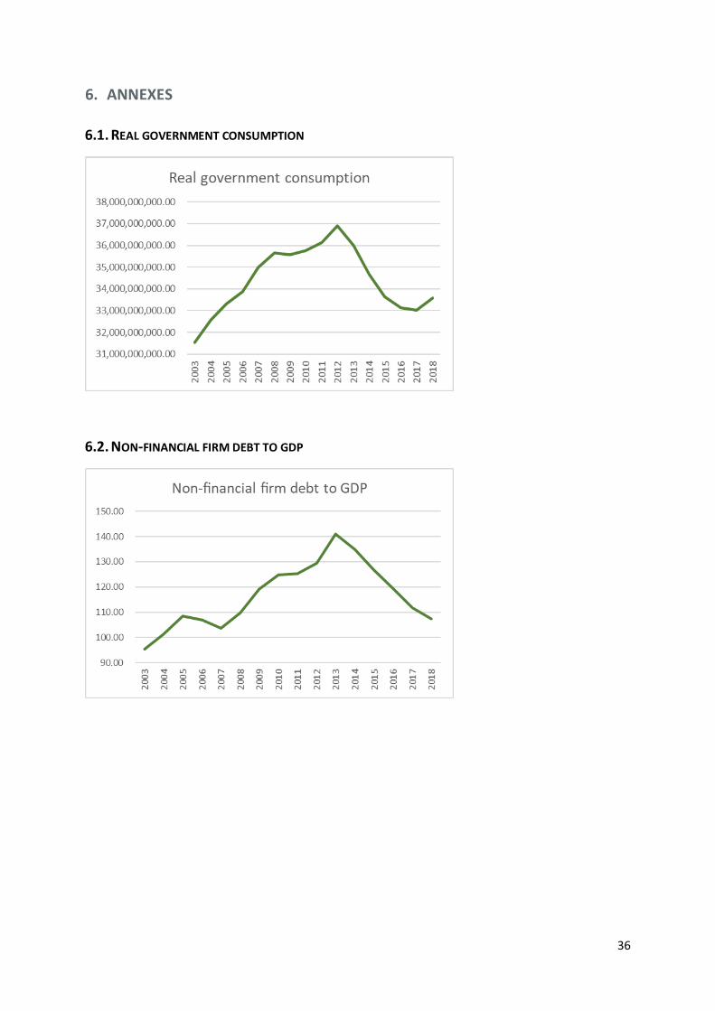
36

6. ANNEXES

6.1. REAL GOVERNMENT CONSUMPTION

6.2. NON-FINANCIAL FIRM DEBT TO GDP

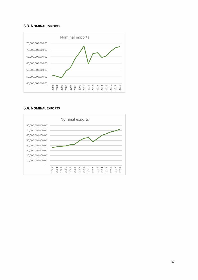
37

6.3. NOMINAL IMPORTS

6.4. NOMINAL EXPORTS

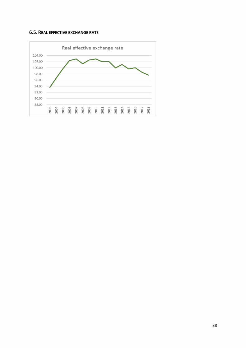
38

6.5. REAL EFFECTIVE EXCHANGE RATE

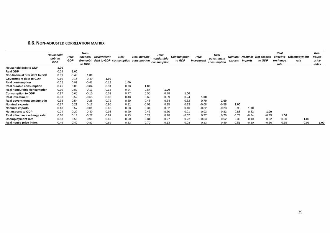
39

6.6. NON-ADJUSTED CORRELATION MATRIX

Household

debt to

GDP

Real

GDP

Non-

financial

firm debt

to GDP

Government

debt to GDP

Real

consumption

Real durable

consumption

Real

nondurable

consumption

Consumption

to GDP

Real

investment

Real

government

consumption

Nominal

exports

Nominal

imports

Net exports

to GDP

Real

effective

exchange

rate

Unemployment

rate

Real

house

price

index


Real GDP -0.09 1.00

Non-financial firm debt to GDP 0.69 -0.49 1.00

Government debt to GDP -0.19 -0.16 0.40 1.00

Real consumption -0.02 0.97 -0.41 -0.12 1.00

Real durable consumption -0.46 0.80 -0.84 -0.31 0.78 1.00

Real nondurable consumption 0.30 0.89 -0.13 -0.13 0.94 0.54 1.00

Consumption to GDP 0.17 0.60 -0.10 0.02 0.77 0.50 0.78 1.00

Real investment -0.03 0.52 -0.65 -0.88 0.48 0.69 0.39 0.24 1.00

Real government consumption 0.38 0.54 -0.28 -0.72 0.59 0.48 0.64 0.52 0.79 1.00

Nominal exports -0.27 0.21 0.17 0.90 0.21 -0.01 0.15 0.13 -0.68 -0.58 1.00

Nominal imports -0.18 0.57 -0.01 0.66 0.58 0.31 0.52 0.40 -0.32 -0.23 0.90 1.00

Net exports to GDP -0.24 -0.29 0.40 0.95 -0.29 -0.43 -0.30 -0.21 -0.93 -0.83 0.85 0.53 1.00

Real effective exchange rate 0.30 0.18 -0.27 -0.91 0.13 0.21 0.18 -0.07 0.77 0.70 -0.78 -0.54 -0.85 1.00

Unemployment rate 0.53 -0.56 0.90 0.60 -0.50 -0.84 -0.27 -0.22 -0.83 -0.52 0.36 0.10 0.62 -0.50 1.00

Real house price index -0.49 0.40 -0.87 -0.69 0.33 0.70 0.13 0.03 0.83 0.49 -0.51 -0.30 -0.66 0.55 -0.93 1.00

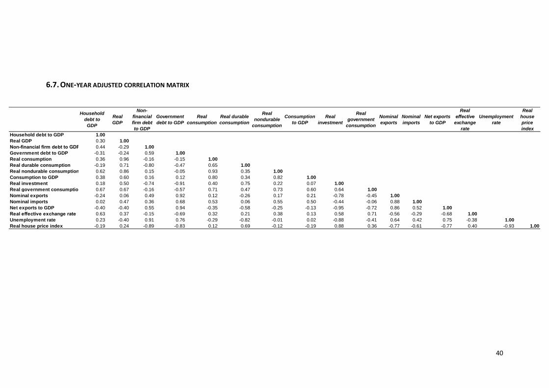
40

6.7. ONE-YEAR ADJUSTED CORRELATION MATRIX

Household

debt to

GDP

Real

GDP

Non-

financial

firm debt

to GDP

Government

debt to GDP

Real

consumption

Real durable

consumption

Real

nondurable

consumption

Consumption

to GDP

Real

investment

Real

government

consumption

Nominal

exports

Nominal

imports

Net exports

to GDP

Real

effective

exchange

rate

Unemployment

rate

Real

house

price

index


Real GDP 0.30 1.00



Real consumption 0.36 0.96 -0.16 -0.15 1.00

Real durable consumption -0.19 0.71 -0.80 -0.47 0.65 1.00

Real nondurable consumption 0.62 0.86 0.15 -0.05 0.93 0.35 1.00

Consumption to GDP 0.38 0.60 0.16 0.12 0.80 0.34 0.82 1.00

Real investment 0.18 0.50 -0.74 -0.91 0.40 0.75 0.22 0.07 1.00

Real government consumption 0.67 0.67 -0.16 -0.57 0.71 0.47 0.73 0.60 0.64 1.00

Nominal exports -0.24 0.06 0.49 0.92 0.12 -0.26 0.17 0.21 -0.78 -0.45 1.00

Nominal imports 0.02 0.47 0.36 0.68 0.53 0.06 0.55 0.50 -0.44 -0.06 0.88 1.00


Real effective exchange rate 0.63 0.37 -0.15 -0.69 0.32 0.21 0.38 0.13 0.58 0.71 -0.56 -0.29 -0.68 1.00

Unemployment rate 0.23 -0.40 0.91 0.76 -0.29 -0.82 -0.01 0.02 -0.88 -0.41 0.64 0.42 0.75 -0.38 1.00

Real house price index -0.19 0.24 -0.89 -0.83 0.12 0.69 -0.12 -0.19 0.88 0.36 -0.77 -0.61 -0.77 0.40 -0.93 1.00

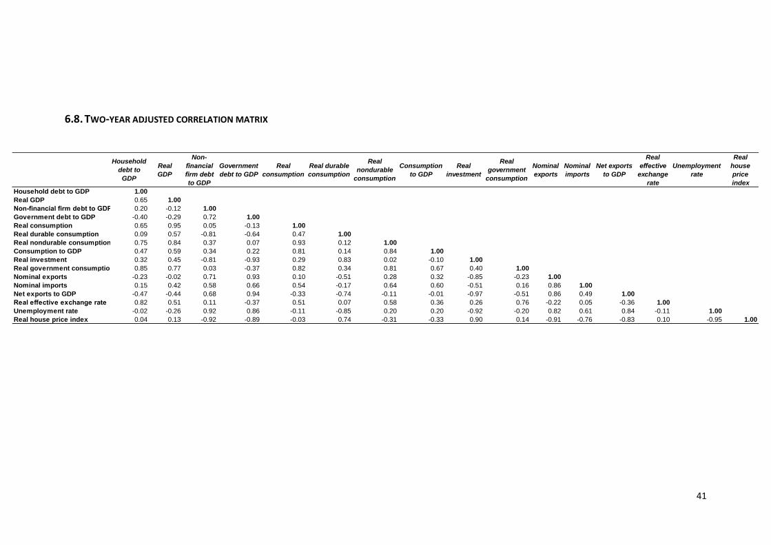
41

6.8. TWO-YEAR ADJUSTED CORRELATION MATRIX

Household

debt to

GDP

Real

GDP

Non-

financial

firm debt

to GDP

Government

debt to GDP

Real

consumption

Real durable

consumption

Real

nondurable

consumption

Consumption

to GDP

Real

investment

Real

government

consumption

Nominal

exports

Nominal

imports

Net exports

to GDP

Real

effective

exchange

rate

Unemployment

rate

Real

house

price

index


Real GDP 0.65 1.00



Real consumption 0.65 0.95 0.05 -0.13 1.00

Real durable consumption 0.09 0.57 -0.81 -0.64 0.47 1.00

Real nondurable consumption 0.75 0.84 0.37 0.07 0.93 0.12 1.00


Real investment 0.32 0.45 -0.81 -0.93 0.29 0.83 0.02 -0.10 1.00

Real government consumption 0.85 0.77 0.03 -0.37 0.82 0.34 0.81 0.67 0.40 1.00

Nominal exports -0.23 -0.02 0.71 0.93 0.10 -0.51 0.28 0.32 -0.85 -0.23 1.00

Nominal imports 0.15 0.42 0.58 0.66 0.54 -0.17 0.64 0.60 -0.51 0.16 0.86 1.00


Real effective exchange rate 0.82 0.51 0.11 -0.37 0.51 0.07 0.58 0.36 0.26 0.76 -0.22 0.05 -0.36 1.00

Unemployment rate -0.02 -0.26 0.92 0.86 -0.11 -0.85 0.20 0.20 -0.92 -0.20 0.82 0.61 0.84 -0.11 1.00

Real house price index 0.04 0.13 -0.92 -0.89 -0.03 0.74 -0.31 -0.33 0.90 0.14 -0.91 -0.76 -0.83 0.10 -0.95 1.00

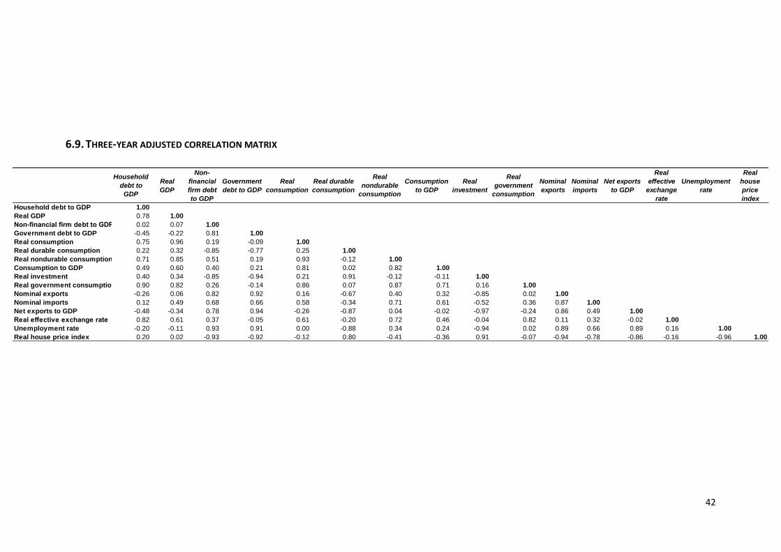
42

6.9. THREE-YEAR ADJUSTED CORRELATION MATRIX

Household

debt to

GDP

Real

GDP

Non-

financial

firm debt

to GDP

Government

debt to GDP

Real

consumption

Real durable

consumption

Real

nondurable

consumption

Consumption

to GDP

Real

investment

Real

government

consumption

Nominal

exports

Nominal

imports

Net exports

to GDP

Real

effective

exchange

rate

Unemployment

rate

Real

house

price

index


Real GDP 0.78 1.00

Non-financial firm debt to GDP 0.02 0.07 1.00


Real consumption 0.75 0.96 0.19 -0.09 1.00

Real durable consumption 0.22 0.32 -0.85 -0.77 0.25 1.00

Real nondurable consumption 0.71 0.85 0.51 0.19 0.93 -0.12 1.00


Real investment 0.40 0.34 -0.85 -0.94 0.21 0.91 -0.12 -0.11 1.00

Real government consumption 0.90 0.82 0.26 -0.14 0.86 0.07 0.87 0.71 0.16 1.00

Nominal exports -0.26 0.06 0.82 0.92 0.16 -0.67 0.40 0.32 -0.85 0.02 1.00

Nominal imports 0.12 0.49 0.68 0.66 0.58 -0.34 0.71 0.61 -0.52 0.36 0.87 1.00

Net exports to GDP -0.48 -0.34 0.78 0.94 -0.26 -0.87 0.04 -0.02 -0.97 -0.24 0.86 0.49 1.00

Real effective exchange rate 0.82 0.61 0.37 -0.05 0.61 -0.20 0.72 0.46 -0.04 0.82 0.11 0.32 -0.02 1.00

Unemployment rate -0.20 -0.11 0.93 0.91 0.00 -0.88 0.34 0.24 -0.94 0.02 0.89 0.66 0.89 0.16 1.00

Real house price index 0.20 0.02 -0.93 -0.92 -0.12 0.80 -0.41 -0.36 0.91 -0.07 -0.94 -0.78 -0.86 -0.16 -0.96 1.00

Documents

Understanding business cycles: credit supply, household