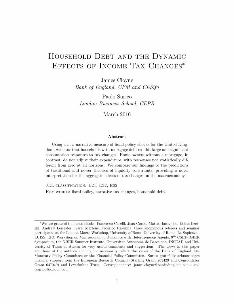
Household Debt and the DynamicEffects of Income Tax Changes∗

James CloyneBank of England, CFM and CESifo

Paolo SuricoLondon Business School, CEPR

March 2016

Abstract

Using a new narrative measure of fiscal policy shocks for the United King-dom, we show that households with mortgage debt exhibit large and significantconsumption responses to tax changes. Home-owners without a mortgage, incontrast, do not adjust their expenditure, with responses not statistically dif-ferent from zero at all horizons. We compare our findings to the predictionsof traditional and newer theories of liquidity constraints, providing a novelinterpretation for the aggregate effects of tax changes on the macroeconomy.

JEL classification: E21, E32, E62.

Key words: fiscal policy, narrative tax changes, household debt.

∗We are grateful to James Banks, Francesco Caselli, Joao Cocco, Matteo Iacoviello, Ethan Ilzet-zki, Andrew Leicester, Karel Mertens, Federico Ravenna, three anonymous referees and seminarparticipants at the London Macro Workshop, University of Bonn, University of Rome ‘La Sapienza’,LUISS, ERC Workshop on Macroeconomic Dynamics with Heterogeneous Agents, 9th CSEF-IGIERSymposium, the NBER Summer Institute, Universitat Autonoma de Barcelona, INSEAD and Uni-versity of Texas at Austin for very useful comments and suggestions. The views in this paperare those of the authors and do not necessarily reflect the views of the Bank of England, theMonetary Policy Committee or the Financial Policy Committee. Surico gratefully acknowledgesfinancial support from the European Research Council (Starting Grant 263429 and ConsolidatorGrant 647049) and Leverhulme Trust. Correspondence: james.cloyne@bankofengland.co.uk andpsurico@london.edu.

1

1 Introduction

The persistent rise in mortgage debt prior to the recent financial crisis has drawn con-

siderable attention to the role of private indebtedness in the transmission of macroe-

conomic shocks in advanced economies. On the empirical side, Mian et al. (2012),

Dynan (2012) and the IMF (2012) report that high levels of household debt are likely

to have amplified and prolonged the Great Recession of 2007–08. On the theoretical

side, Eggertsson and Krugman (2012), Andres et al. (2012) and Kaplan and Violante

(2014) present heterogeneous agent models where fiscal policy is more effective the

larger the proportion of debt-constrained households.

A common presumption behind these studies is that debtors are more likely to face

liquidity constraints and therefore adjust their consumption significantly in response

to conditions that unexpectedly change their income. An important implication is

that it is not net wealth per se that determines the consumption response to fiscal

policy: households who made a large durable purchase, such as housing, may well

be wealthy and liquidity constrained at the same time. Despite the importance of

this transmission mechanism for both policy and academic research, little is known

empirically about whether the effects of tax changes on consumption vary with a

household’s debt position.

Looking at the empirical association between consumption, income and debt is

complicated by at least three factors. First, since consumption and income are jointly

determined we need to isolate the exogenous component of income changes. Second,

survey data with good coverage of expenditure typically lack equally detailed and

reliable information on wealth over a sufficiently long period of time. We therefore

need to identify a proxy for the household debt position. Third, commonly used

surveys are either repeated cross-sections, like the Family Expenditure Survey for the

U.K., or overlapping panels with a short time series dimension, like the Consumption

Expenditure Survey for the US. We therefore need to group individual observations

into aggregate pseudo-cohorts.

To address the endogeneity of income changes, we identify exogenous variation in

2

taxes using the narrative approach pioneered by Romer and Romer (2010) and applied

to aggregate tax changes in the United Kingdom by Cloyne (2013). More specifically,

we construct a new series of changes in household income tax for the U.K. that are

exogenous to both macroeconomic and cohort-level fluctuations. The U.K. appears

a natural choice for our purposes because there have been a large number of income

tax changes in the last forty years and detailed official documents allow us to identify

individual tax measures and their motivations.

To elicit individual debt positions, we propose to group households by housing

tenure (whether households are mortgagors, outright owners or renters) using the UK

Family Expenditure Survey (FES) and compare the consumption response of home-

owners with mortgage debt with the response of outright home-owners (i.e. those

without a mortgage). The motivation for this novel grouping strategy is threefold.

First, mortgages are the most prominent form of household debt, in both incidence

and value. Second, the extensive margin of whether a household holds a mortgage

is likely to be less prone to measurement errors than the intensive margin of its

outstanding value (which is recorded consistently in the FES only over a shorter

period of time). Third, looking at housing tenure allows us to investigate the dynamic

effects of tax changes on the consumption of ‘social renters’ (i.e. those renting from

local authorities or housing associations). This is a group with virtually no net

wealth, low income and only compulsory education and therefore fits the traditional

stereotype of liquidity constrained households in one-asset models.1

A potential drawback of grouping households by their housing tenure status is the

possibility of endogenous transitions from one tenure status to another over time as

a result of any tax change. The very gradual rate at which ownership has risen in the

United Kingdom suggests this may be less of a concern. But, to verify this, we show

that our results are robust to using the grouping strategy proposed by Attanasio et al.

(2002), which explicitly addresses the possibility of endogenous movements between

1It is worth noting, however, that social renters account for only around 20% of the Britishpopulation and thus they seem unlikely, on their own, to account for the large and persistent effectsof tax changes on the aggregate economy typically found in empirical macro studies.

3

groups and compositional change.

A more significant limitation of our empirical design is that households in our

sample are not randomly assigned to mortgagor, outright owner, or social renter

status. Indeed, we document some systematic differences between these groups, for

instance in terms of demographics and educational attainment, suggesting the pos-

sible presence of a selection issue: mortgagors may be responding differently from

outright owners not because they have a mortgage, but because some other trait that

makes households more responsive to tax changes is present disproportionately in the

mortgagor population. Nevertheless, it is difficult to identify obvious candidates for

such a trait, especially in light of our findings that the response by outright owners is

insignificant and small, that the heterogeneity in the consumption adjustment across

birth and education cohorts is limited, and the fact that we also present additional

results which line up, quantitatively and qualitatively, with the theoretical predic-

tions of a model based on liquidity constraints (but tend to accord less well with the

predictions associated with alternative explanations). Furthermore, even if we were

unable to establish conclusively that the effect of the tax cut is due to liquidity con-

straints, our results may have important policy implications in that they highlight a

new variable (mortgagor status) which performs exceptionally well in identifying the

group of population most likely to respond to policy changes.

This paper makes two main contributions to the fiscal policy literature. First,

we document that the dynamic effects of exogenous income tax changes on private

consumption are highly heterogeneous across housing tenures: mortgagors exhibit

the largest and most significant response, outright home-owners hardly adjust their

expenditure at all and social renters change their consumption somewhat less than

mortgagors. Second, we provide empirical support for the notion that household

mortgage debt positions play a role in the transmission mechanism of fiscal policy.

Specifically, as noted above, we show that our findings are consistent with the qual-

itative and quantitative predictions of a consumption model where accessing illiquid

wealth (such as housing) is subject to transaction costs. Since mortgagors tend to

4

account for between 40% and 50% of the population over the sample, our evidence

suggests that this new type of liquidity-constrained household can make a substantial

contribution to the large effects of tax changes reported in earlier empirical macro

studies.

Related literature. This paper contributes to a growing body of empirical re-

search on consumption heterogeneity, including Anderson et al. (2012), De Giorgi

and Gambetti (2012a), Ercolani and Pavoni (2012) and Misra and Surico (2014)

among others. The findings from these studies have been interpreted as supportive

of theories of precautionary saving, partial insurance and limited participation. Our

results highlight the role of an additional channel in the transmission of structural

shocks: mortgage debt positions. This appears consistent with a framework where the

decision to purchase a large durable good through borrowing makes some households

‘wealthy’ hand-to-mouth, as in Kaplan and Violante (2014).

Our results also relate to a range of empirical contributions on the macroeconomic

effects of fiscal policy on real activity. While our estimates are consistent with those

reported by Romer and Romer (2010), Mertens and Ravn (2012), Caldara and Kamps

(2008, 2012), Mountford and Uhlig (2009) and Cloyne (2013), among others, our

approach allows us to identify which households drive the aggregate result as well as

which individual characteristics tend to predict a higher sensitivity of consumption

to income changes.

While we consider the heterogeneous effects of income tax changes, another strand

of the literature has looked at the heterogeneous effects of government spending

across different industries (Nekarda and Ramey (2011)), the state of the business

cycle (Auerbach and Gorodnichenko (2012, 2013), Owyang et al. (2013)) and across

households (Giavazzi and McMahon (2012), De Giorgi and Gambetti (2012b)).

Paper layout. Our analysis is structured as follows. Section 2 presents our new

series of narrative-identified tax changes and describes how we use the household

survey data to construct expenditure measures by housing tenure. Section 3 finds

5

pervasive heterogeneity in the consumption responses to tax changes across housing

tenures and demonstrates robustness across an extensive list of modifications to our

baseline specification. Section 4 examines the relationship between mortgage debt

and liquidity constraints, and the extent to which this is consistent with our findings.

We show that this channel compares favourably with the alternative explanations

assessed in Section 5. The Appendices contain a description of the data and further

econometric results. A Supplementary Appendix presents the narrative evidence

supporting the construction of our exogenous income tax series.

2 Identification

In this section, we present our identification strategy and the data sets we employ.

We first discuss the narrative data on UK tax changes and the way we exploit these

to construct an exogenous income tax measure. We then move to the household

survey data and the grouping strategy used to construct time series of consumption

for pseudo-cohorts based on housing tenure status.

2.1 UK income tax changes and the narrative approach

A key identification challenge we face is that tax changes may affect consumption

and other macroeconomic variables but common measures of taxes are also affected

by the state of the economy. This may be because tax revenues are affected auto-

matically by the cycle or because discretionary policy actions are taken in response

to macroeconomic or cohort-level economic conditions. Since our household tenure

groups are large shares of the population, the simultaneity between fiscal policy and

consumption prevents consistent estimation.

To address the identification problem, we employ a narrative approach following

Romer and Romer (2010) for the United States and Cloyne (2013) for the United

Kingdom. We use detailed documentation from historical sources to identify ‘exoge-

nous’ legislated changes in tax policy from the motivations given by lawmakers at

6

the time of the policy intervention.2 Unfortunately, the narrative measures of aggre-

gate tax changes used in earlier contributions contain changes to a variety of taxes

such as income, consumption and capital taxes, each of which may affect household

groups differently (e.g. Stamp Duty, Vehicle Excise Duty etc). Ideally, we seek tax

changes that affect all housing tenure groups. We therefore focus on specific changes

to household income taxes.

Income tax in the U.K. is payable on a wide range of income including earnings

from employment, property, interest, retirement pensions and some social security

benefits. Further details of the UK income tax system are provided in Appendix A.

To focus on changes that affect all income taxpayers, we collect a data set of changes

affecting the lowest bracket of income tax. Specifically, we consider changes in the tax

free allowances (that determine the level of income above which income tax starts to

be paid), the basic rate of income tax (currently 20 per cent) and the income bands

defining the basic rate. We refer to this group of tax changes as the allowance and

basic rate of income tax.3

Our starting point is the narrative record of tax interventions in the U.K. reported

by Cloyne (2012). More specifically, we work back through all the original documents

to collect the specific set of income taxes. While some of this information is already

contained in Cloyne (2012), in many cases there is not enough detail for our new

purpose. For instance, the types of tax changes (e.g. allowances and basic rate

changes) are not specifically categorised in a manner that is readily suitable for our

purpose.

Our narrative analysis isolates around 140 changes in the allowances and basic

rate of income tax.4 For the quantitative magnitude of each change, we follow Romer

2The idea has been applied to government spending (Ramey and Shapiro (1998); Ramey (2011)),monetary policy (Romer and Romer (1989, 2004)) and fiscal consolidations (Guajardo et al. (2011)).

3Mertens and Ravn (2013) split the Romer and Romer dataset into corporate and personal taxliabilities and study the macroeconomic effects of these tax changes. As we examine sub-groups ofthe population, we need to construct a more specific measure of income tax changes.

4This measure is even more conservative than the narrative series used in Cloyne and Surico(2013) as we drop a small number of tax changes that, while not explicitly directed to a specifichousing tenure group, might be argued to have affected unevenly other (small) groups in society.

7

and Romer (2010) and use the revenue forecasts from the Budget documents. The

focus is on the change in tax liabilities rather than any short-run revenue effect due

to the timing of revenues reaching the Treasury. Consequently we use the ‘full year’

revenue estimate, which is the projected on-going annualised effect on tax liabilities.

This value is assigned to the implementation date of the policy change. The main

sources for the policy changes and revenue estimates is the Financial Statement and

Budget Report (FSBR) which is published alongside the Budget speech. As explained

by Mertens and Ravn (2012), the implementation date might be anticipated whenever

the policy announcement takes place some time before its implementation. We ad-

dress this possibility in Section 3 and show that our findings are robust to considering

only tax changes implemented on announcement.

As in Romer and Romer (2010) and Cloyne (2013), we categorise all the indi-

vidual tax changes as either exogenous and endogenous based on whether they were

motivated as a response to changing macroeconomic conditions (for example, GDP,

consumption or other spending decisions). Unlike Cloyne (2013), however, we also

examine whether the policy changes followed fluctuations in the circumstances of

particular housing tenure groups. Our new measure is therefore also exogenous to

developments in these specific cohorts. Much more detail regarding the sources, meth-

ods and supporting narrative evidence can be found in the Supplementary Appendix.

Here, we briefly note that, in categorising the given motivations, we use a variety of

UK government, parliamentary and historical documents and speeches. The main

source is either the Chancellor’s Parliamentary speech recorded in Hansard (the of-

ficial parliamentary record), or the Economic and Fiscal Strategy Report (EFSR)

published with more recent Budgets.

Individual exogenous income tax changes are assigned to quarters and aggregated.

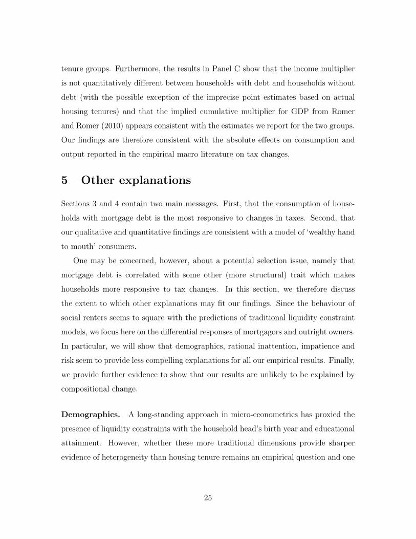
Figure 1 shows, as the solid line, our newly compiled tax series scaled by nominal

GDP, together with the aggregate tax change series in Cloyne (2013) as the dashed

line. There have been a sizable number of income tax changes and many of these have

been quite large, providing good variation in our narrative tax series over time. The

8

large majority of these legislated changes were reforms designed to encourage long-

run economic performance, sharpening incentives and lowering the overall burden

of taxation. Reassuringly, the correlation between all other exogenous income tax

changes and our measure of changes to the allowance and the basic rate is low, at

0.15. Similarly, the correlation with all other exogenous tax changes is −0.07. This

suggests that changes in our measure were not contemporaneously offset by changes

in the higher rates of income tax.

Two features of the narrative construction of a tax shock series are worth em-

phasizing. First, the official Budget documents report projections for the change in

annual tax liabilities as a result of the legislated policy action (rather than the ab-

solute effect on the levels). Second, narrative-identified tax shocks (including ours)

tend to exhibits virtually no persistence. These two features imply that the empirical

model, discussed below, mechanically simulates the dynamic effect of a one pound

tax cut as a shock that lowers, by one pound, the level of taxes paid in each year

of the forecast period.5 Given the frequency with which income taxes have changed

over our sample period, however, it would seem difficult to interpret our shocks as

permanent.

In Romer and Romer (2010) and Cloyne (2013), the tax measure can be thought

of as the change in an aggregate average tax rate. For our purpose, however, it makes

less sense to divide income tax liabilities by aggregate GDP as this would not reflect

an average tax rate. Instead, we transform our nominal tax liabilities series into a

(real) income tax change per taxpayer. We divide the (narrative) projected change

in nominal liabilities by the Retail Prices Index (RPIX) and the total number of

individual income taxpayers. Over a three year horizon, this amounts to an average

tax change of about 700 pounds sterling per household at 2009 prices.

5In contrast to Mertens and Ravn (2013) for the US, tax revenue data for the UK are not suf-ficiently detailed to construct a National Accounts quarterly counterpart of the specific subgroupof income taxes we consider (nor the tax base) over a long period of time. We have verified, how-ever, that our measure generates persistent movements in total income tax revenues (from NationalAccounts) as a share of GDP, although the estimates become less precise at longer horizons.

9

Cohort-specific Granger Causality Tests. The narrative account in the Supple-

mentary Appendix suggests that our newly constructed income tax changes should, if

truly exogenous, be unpredictable on the basis of either cohort-specific or macroeco-

nomic conditions and we now verify this. Specifically, we conduct Granger causality

tests based on a VAR which contains the change in consumption and income per

capita for each household group, the change in real GDP and government spending

per capita, the central bank’s policy rate, the change in the FTSE and RPIX inflation.

Reassuringly, we could not reject the hypothesis that the cohort-specific variables do

not Granger cause our income tax series: the p-values using various lag lengths were

high, over 0.4, for 4, 6 and 8 lags.

2.2 Household consumption data

The focus of our analysis is on whether households with mortgage debt respond more

to income tax changes than those without. For this purpose, we need both good

quality household expenditure data and information on household debt positions.

Household expenditure data are obtained using 32 waves, from 1978 to 2009, of the

Living Costs and Food Survey, commonly known as the Family Expenditure Survey.

This survey has high quality, detailed information on expenditure and household char-

acteristics.6 Each wave contains around 7,000 households, generating over 200,000

observations in total (see Appendix B).

Ideally, we would like to observe individual balance sheet positions and expen-

diture. Unfortunately, there are no micro data sets that jointly record detailed in-

formation on consumption and wealth over a sufficiently long time period and the

FES is no exception. To construct a pseudo-panel, it is therefore common to use a

grouping estimator along the lines proposed by Browning et al. (1985). Given our

focus on mortgage debt, housing tenure appears a natural dimension to aggregate

households in three pseudo-cohorts, therefore bypassing the lack of household debt

data. Since loans secured on housing represent the majority of household debt, we

6While the survey has run from 1968, educational attainment is only available from 1978.

10

are particularly interested in whether home owners with mortgage debt react more

to tax changes than home-owners without.

As another interesting group, we consider a third tenure category: those living in

accommodation rented from local authorities or housing associations. For short, we

refer to these households as ‘social renters’. These households tend to be poorer, have

only compulsory education and — as we will show using less frequent data from the

British Household Panel Survey — have little liquid or illiquid wealth.7 The social

renters therefore fit the demographic characteristics of those more likely to be credit

constrained in the traditional sense used in earlier empirical contributions. For this

reason, we see the ‘social renter’ group as a useful comparison.

We focus on non-durable goods and services expenditure. Since we examine the

response of consumption to tax changes, we only want to include taxpayers in our

sample. The FES contains information on income taxes paid and we therefore exclude

households who reported they did not pay any tax. However, there may be some

measurement error associated with this reporting. After excluding these households,

we also then drop any remaining households whose income was below the threshold

for paying income tax.8

In our sample, mortgagors represent about 45% of the observations, on average,

while social renters and owners outright represent around 20 % and 25 % each. Private

renters averages around a 10% share but over several quarters around the middle of

the sample their number appears too low (below sixty) to draw any reliable inference

and are therefore excluded.

Each household is assigned to a quarter based on the date of the interview. To

account for some (unrealistically) high or low values of consumption, for each quarter

and tenure group we drop the top and bottom 1% of observations.9 Then, we sum-up

7Unlike the FES, the BHPS has limited consumption coverage, mostly on food expenditure.8These two strategies largely identify the same group of households, whose dominant share

(around 70%) is made of social renters. Non-tax paying social renters represent about 40% of thetotal number of social renters in the whole FES sample. We have verified that the non-taxpayers’consumption response to our income tax shock is never statistically different from zero.

9Similar but less precise estimates for the unrestricted sample are in Cloyne and Surico (2013).

11

the individual survey responses within each cohort by quarter using household weights

that ensure representativeness in the British population, divide by the number of

people in the household to generate a per capita measure and divide by the retail

prices index excluding mortgage repayments (RPIX). To address seasonality, we use

the annual change in quarterly expenditure for each group.

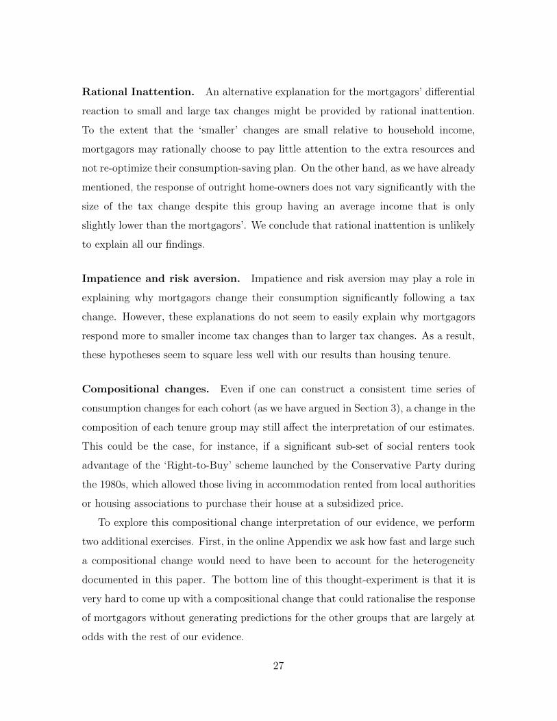
One issue using a grouping estimator is that the dimension along which the ag-

gregation is performed needs to be fully predictable over time. In our case, we do

not know whether a household with a particular tenure status had the same tenure

status in the previous period or whether it will still have the same tenure status in

the next period. Figure 2 shows that there has been some variation in the shares of

the tenure groups over time, especially before 1986, although the dynamics of these

series appear to be relatively slow moving. To ensure robustness of our findings, we

also consider grouping households according to their predicted probabilities of having

a mortgage based on exogenous observables. More specifically, in the next section, we

complement the evidence using actual housing tenure groupings with results based

on the propensity score grouping strategy proposed by Attanasio et al. (2002). We

also assess the sensitivity of our findings to using shorter samples that start between

the mid-1980s and the early 1990s which, according to Figure 2, were characterized

by a greater stability in the evolution of tenure shares.

Before turning to the estimation, it is useful to examine the demographic proper-

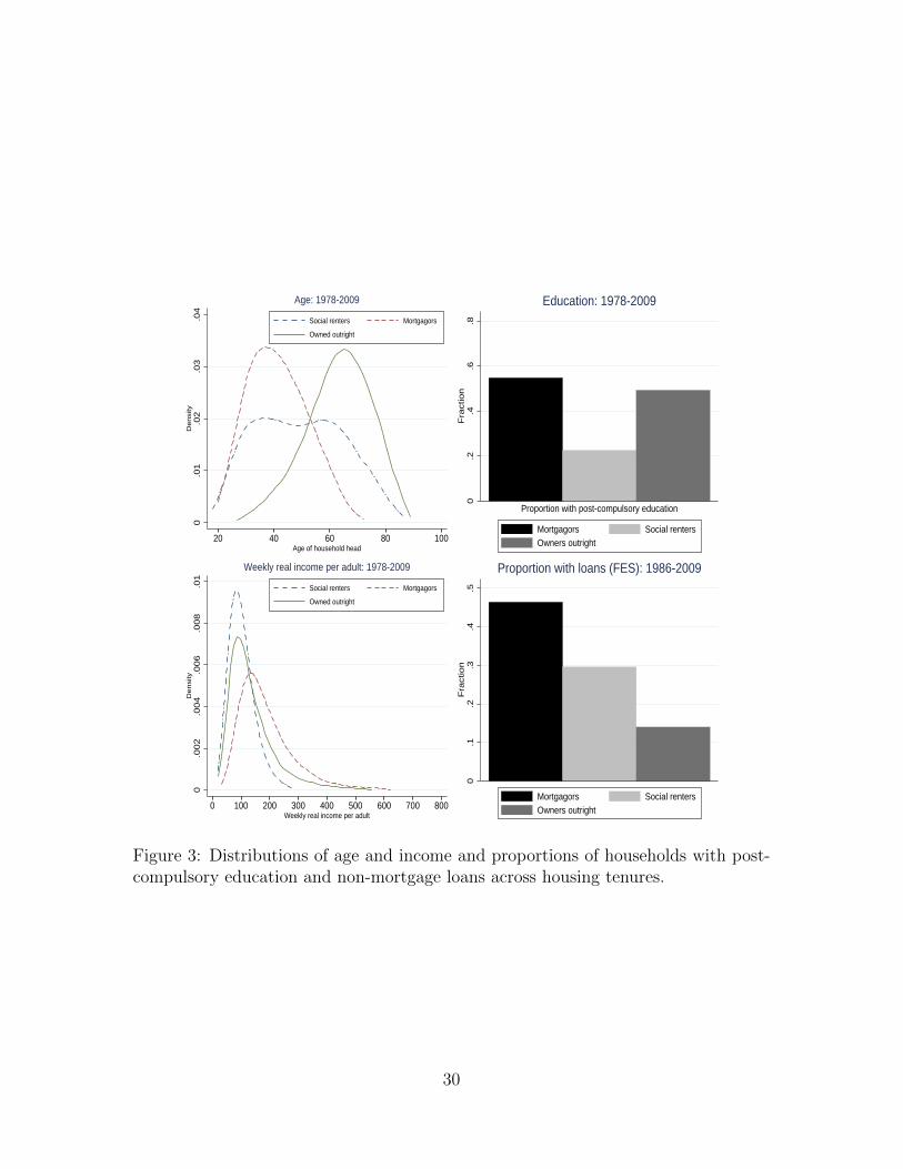
ties of our pseudo-cohorts. For each group, Figure 3 shows kernel density estimates

of age (i.e. the difference between interview year and household head’s birth year)

and weekly household real income per adult as well as the shares of households with

different education levels and the shares of households with positive non-mortgage

debt. Mortgagors were born on average in later years (so tend to be younger in our

sample), tend to be more educated and appear relatively richer. It is worth noting,

however, that the distributions of the three tenure groups overlap significantly.10 In

particular, the estimated densities for both groups of home owners are characterised

10A similar picture emerges considering household disposable income.

12

by a long right tail. This means that average income of outright owners is relatively

closer to the average income of mortgagors rather than social renters.11 Finally, the

mortgagor group has the largest share of households with positive non-mortgage debt

while outright owners have the lowest.12

3 The heterogeneous effects of tax changes

In this section, we document significant heterogeneity in the dynamic effects of fiscal

policy by reporting the estimated consumption responses across actual housing tenure

groups. To assess concerns of possible endogenous changes in group composition, we

then show that our findings are not overturned when households are grouped accord-

ing to their predicted probability (based on a nonlinear polynomial in demographics,

education and time trends) of having the same housing tenure status in the previous

year (which we do not observe in the repeated cross-sections of the FES).

For each tenure group, we estimate a separate Vector Autoregression (VAR). The

VAR includes the change in group-specific consumption, the change in real GDP, the

level of the central bank’s policy rate and the change in real government spending.

We use four lags of these endogenous variables.13 In line with the empirical literature

on narrative measures of fiscal shocks, the first twelve lags and the contemporaneous

value of our newly compiled exogenous measure of income tax changes enter the VAR

as exogenous variables. The contemporaneous values of the share of households with

post-compulsory education and the average difference between interview year and

birth year in each quarter are added as further exogenous regressors to control for

other unrelated life-cycle factors. In Cloyne and Surico (2013), we show that the

results below are robust to running the single equation specification used in Romer

and Romer (2010) as well as to using the method of Seemingly Unrelated Regressions.

11The sub-sample evidence in Appendix C reveals that the distributions of education and agehave not changed much over time. In contrast, income has become more unequal, although thishas largely been a feature of the top of the income distribution. Consequently, it has affected theaverage income of the owners and mortgagors but less so the average income of social renters.

12This is based on the shorter FES sample 1986-2009 for which non-mortgage debt is available.13Similar results are obtained using shorter or longer lag lengths.

13

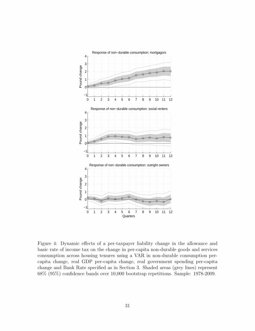
3.1 Actual housing tenure

The point estimates of the dynamic effects of the income tax cut on non-durable

expenditure for each housing tenure group are reported in Figure 4 as solid lines with

circles. The shaded area represents the 68% confidence intervals based on 10,000

bootstrap repetitions; the grey lines show the 95% intervals.

Each point of the impulse response function represents the effect on annual con-

sumption following a one pound tax change, relative to what would have happened

in the absence of the shock.14 Since our shock series reflects changes in taxes, this is

equivalent to a shock that lowers the level of taxes by one pound in each of the three

years of the forecast period. The response at the end of each year can therefore be

seen as the fiscal multiplier in that year of the simulation, although — as discussed

in Section 2 — we do not regard these tax changes as permanent.

The first row shows that the consumption of mortgagors responds significantly

at the 5% level beyond the third quarter and reaches a peak around 2 pounds after

three years. In contrast, the response of owners without mortgage (in the last row) is

never statistically different from zero, even at the 32% significance level, and peaks

below 0.4 or 40 pence at six quarters after the shock. Finally, the point estimates

in the second row suggest that social renters change their non-durable expenditure

by slightly less than one pound, with responses that are significant at 5% between

quarters 3 and 6.15 As owners without a mortgage tend to have a significantly higher

gross income than social renters, it seems unlikely that the heterogeneity in Figure

4 is driven by possible heterogeneity in the tax change, although we return to this

issue in the sensitivity analysis below.

Turning to the overall magnitudes, the peak effect for mortgagors is equivalent

to a peak fiscal multiplier on consumption of 2 in the third year. The associated

14The response of annual consumption is constructed by cumulating the impulse response func-tion for the annual change in quarterly expenditure, which was estimated using VAR specificationdiscussed above.

15The finding of heterogeneity across groups is robust to using the log difference of consumption,as opposed to the consumption change. Under this transformation, however, the size of the responsesare difficult to interpret as we only observe the tax liability changes projected by HM Treasury.

14

cumulative multiplier over three years (i.e. the overall change in consumption relative

to the overall changes in taxes) is 1.29. It is important to note that these numbers

reflect the general equilibrium effect of the tax stimulus on the economy: Appendix

E shows that income also responds strongly (roughly twice as much as mortgagors’

consumption), with cumulative multipliers for household income between 2 and 3

depending on the specification. Importantly, income moves for all tenure groups

but, as we will show in Section 4, the relative response of consumption is large and

significant for mortgagors but not for outright home-owners. In that section, we

also show that the absolute magnitudes of our estimates are consistent with the tax

multipliers typically found in macroeconomic narrative studies such as Romer and

Romer (2010).

In summary, our estimates suggest that housing tenure is highly correlated with

the characteristics that drive the heterogenous response of household consumption to

an exogenous income tax change. Specifically, whether a household has mortgage debt

seems an important candidate for explaining how tax changes affect consumption. In

Section 4, we will show that the composition of the mortgagors’ asset portfolio — in

particular the lack of significant liquid net wealth — could indeed make this group

more responsive changes in their income.

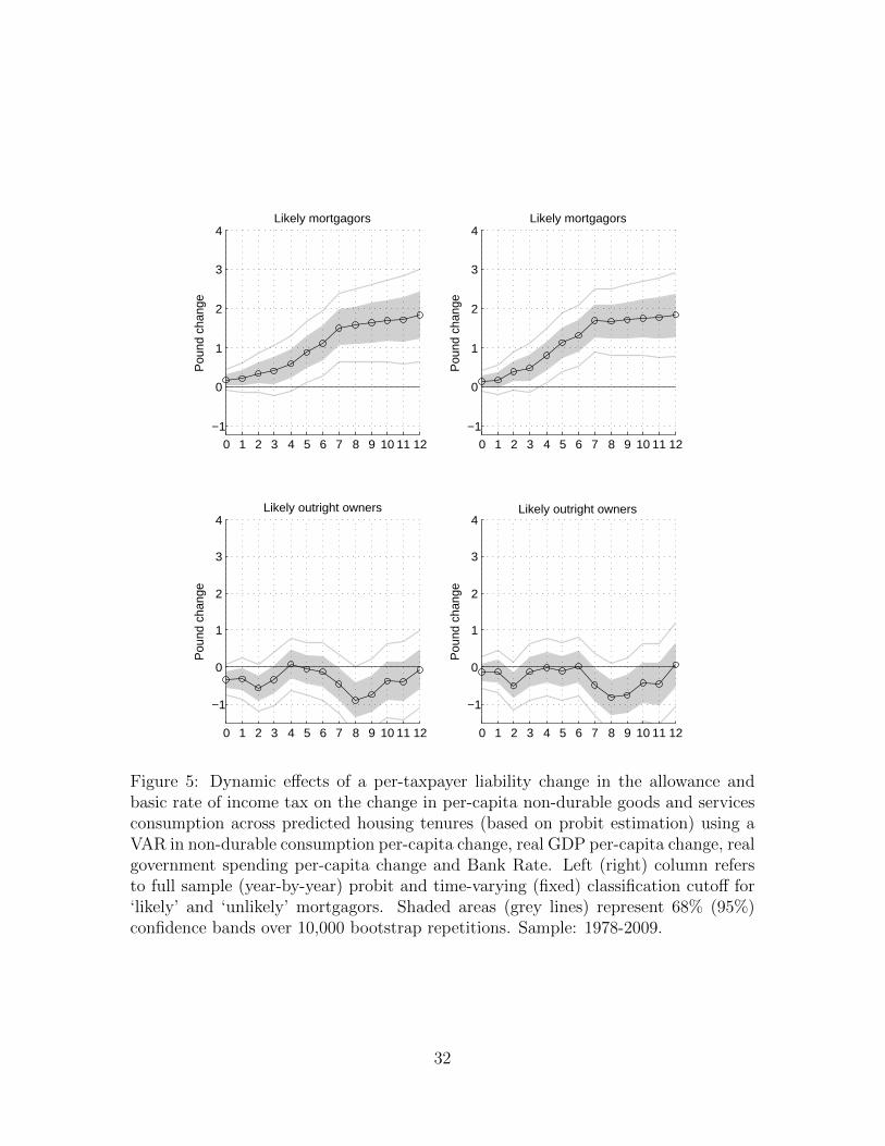
3.2 Propensity score methods

The shares of social renters, mortgagors and outright owners have varied slowly over

time, as shown in Figure 2. Still, if households have chosen to move to another

housing tenure status in response to the fiscal shock, this may distort our inference.

Furthermore, the changes in the time series of consumption that we construct for each

pseudo-cohort can only make sense in the absence of significant compositional changes

across housing tenure groups. To assess the empirical relevance of these concerns, we

adapt the methodology proposed by Attanasio et al. (2002) to generate individual

predicted probabilities of having mortgage debt over a number of subsequent periods.

Specifically, we run a probit regression over the full sample to generate individual

15

predicted probabilities of having a mortgage based on a high order polynomial in

age, education, a time trend and their interactions. For households observed in

quarter t, we compute the probability that they had a mortgage four quarters earlier.

For these two periods, we classify households as ‘likely’ or ‘unlikely mortgagors’ if

the probability in the first of the two periods is larger or smaller than the share of

mortgagors in that period. We then take the difference in consumption across these

two quarters for each group.

By running the probit specification over the full-sample and opting for a time-

varying threshold, the propensity score method of Attanasio et al. (2002) is tailored

to minimize the effects of endogenous changes across tenure groups and classification

errors. However, the composition of the likely mortgagor group may still change

either because the probability of ownership changes over time or because the cutoff

point changes. To deal with this second set of issues, we follow the recommendations

in Attanasio et al. (2002) and run also a probit regression for every year of our sample

and, more importantly, we use a fixed cutoff equal to the average share of mortgagors

in the total population over the full sample, although we have verified that the results

below do not hinge upon the specific value chosen. By using a classification threshold

that does not vary with time, the method minimizes the possible biases induced by

changes in group composition. To make the contrast between outright owners and

mortgagors sharper we have excluded renters from this exercise.16

The results of this exercise are displayed in Figure 5. The left column reports

estimates that use a full-sample probit regression and a time-varying cut-off while

the right column refers to impulse responses that address possible compositional

changes using year-by-year probit regressions and a fixed threshold. Consistent with

the evidence based on actual housing tenure, the response of the ‘unlikely’ mortgagors

is never significant at the 5% level. In contrast, the response of the ‘likely’ mortgagors

remains significant at the 5% level after four quarters and, in line with the estimates

in Figure 4, peaks at around 2 after three years. It is still the case that the 95%

16In Cloyne and Surico (2013), we report similar but less precise estimates when including renters.

16

confidence bands for the likely mortgagors do not include the point estimates for the

unlikely mortgagors after six quarters. We therefore conclude that the heterogeneous

consumption responses between households with and without mortgage debt is robust

to presence of possible endogenous changes in group composition.17 We return to the

issue of compositional change in Section 5.

Income also responds for both groups, as shown in Appendix E. In fact, using the

propensity score method, the income response is very similar for likely and unlikely

mortgagors, reinforcing the result that the differential responses of consumption are

not driven by differential movements in income. We discuss this further in Section 4.

3.3 Sensitivity Analysis

We now conduct a range of sensitivity tests to ensure the robustness of our main

results. For brevity, we list here the main findings and report the full set of results

in the Appendix.

Other tax changes. In considering a subset of tax changes, one possible concern

is that these are correlated with other tax changes whose omission may then distort

our inference. In Figure 9 of the Appendix, we show that our findings are robust to

adding the first twelve lags and the contemporaneous values of any other exogenous

tax changes identified by the narrative method. Furthermore, we have verified that

our shock series does not trigger a significant response of these other tax changes over

the three year forecast period.

Anticipation. One issue is whether the tax changes we consider were anticipated.

In Figure 10, we therefore re-estimate the baseline specification but use the ‘unan-

17In the online Appendix, we use the yearly panel dimension of the British Household Panel Survey(BHPS) between 1991 and 2009 — when the BHPS starts and when our sample ends respectively —to verify that our tax shocks do not have statistical power predicting whether a household changeshousing tenure. Similarly, using the FES over our full sample at quarterly frequency, our taxshocks do not predict whether a household belongs to a specific tenure group. Furthermore, in bothregressions, the coefficients on age, family size and educational attainment are very significant butthe adjusted R2 is never above 0.04 for the BHPS and 0.2 for the FES.

17

ticipated’ component of our exogenous income tax changes. We follow Mertens and

Ravn (2012) by defining an unanticipated change as one that was implemented within

90 days of announcement. The evidence from this exercise suggests that our earlier

findings are broadly confirmed.18

Sub-sample stability. Another sensitivity test is to analyse whether the shape of

the responses for each group varies over time. In Figure 11, we show that this is not

the case by looking at estimates over increasingly shorter samples that start in 1986,

1988, 1990 and 1992 respectively. These years have been chosen as beginning of the

sub-sample because, according to Figure 2, the largest changes in the housing tenure

status occurred between the 1980s and the early 1990s.

Spending categories. Figure 12 shows that excluding semi-durable categories

(such as ‘apparel’, ‘health’ and ‘reading’) from non-durable goods and services in

the second column of ‘strictly non-durables’ does not affect the heterogeneity or the

size of the consumption responses, suggesting our main findings are not driven by the

more durable component of non-durable expenditure. In addition, we record larger

(and far less precise) point estimates for the responses of non-housing expenditure,

but these do not seem statistically different from the responses in Figure 4. Interest-

ingly, Figure 12 also shows that spending on necessities such as food hardly responds

across the three housing tenure groups.

Size of the tax change. Finally, to examine the extent to which our findings may

reflect (omitted) heterogeneity in income, we use the cohort-specific average level

of income to construct a measure of the exogenous tax liability change that reflects

possible variation in the tax base and, therefore, in the average income tax rate across

housing tenure groups. Figure 13 shows that our earlier findings of heterogeneity are

robust also to this exercise.

18Unfortunately, there are only seven tax changes over our full sample which can be deemed asanticipated — too few to be able to carry out a similar analysis for this subgroup.

18

4 Exploring the role of mortgage debt

In the previous section, we documented substantial heterogeneity in the consumption

responses to tax changes. In this section, we provide evidence that our findings

are consistent with a model where liquidity constraints are associated with having

mortgage debt.

We begin by summarizing some of the main testable predictions from a recent the-

oretical framework developed by Kaplan and Violante (2014) and then confront these

predictions with the data. In this model, there are transactions costs associated with

accessing illiquid wealth, and this would make households with mortgage debt more

responsive to income tax changes. We go on to show that our estimates are consistent

with the magnitudes reported in earlier empirical and theoretical contributions on the

effects of fiscal policy. In contrast, in the next section, we argue that alternative hy-

potheses, including demographics, impatience, rational inattention, risk-aversion and

compositional changes are unlikely to fit all our findings.

4.1 Insights from a model of hand-to-mouth households

A popular explanation for the sizable effects of fiscal policy found in the empirical

literature is that a fraction of households are hand-to-mouth, meaning they consume a

significant fraction of any additional income they receive. The conventional wisdom

is that these households are typically renters, have a young household-head, have

lower educational attainment and are on a low income. While this view is often

entertained in policy and academic circles, it has been shown that for an empirically

plausible fraction of these households (typically around 10%), the standard one-asset

model has a hard time replicating the sizable consumption response of households to

a fiscal stimulus (once the model distribution of net worth is calibrated to match the

distribution observed in the data).

To tackle this challenge, Kaplan and Violante (2014) propose a partial equilib-

rium model of consumption in which households can store wealth in two forms: a

liquid asset (such as bank accounts) and an illiquid asset (such as housing). The

19

crucial feature of their framework is that the illiquid asset carries an exogenously

higher rate of return but can be accessed only by paying a transaction cost. When

this assumption is built into an incomplete-markets life-cycle economy, Kaplan and

Violante (2014) show that a significant fraction of households optimally choose to

spend a large fraction of any positive change in their income, despite holding sizable

amounts of illiquid wealth. The intuition is that the welfare loss of not smoothing

consumption turns out to be smaller than the cost of accessing their illiquid wealth

or of holding large balances of cash and foregoing the higher return on the illiquid

asset. They refer to these agents as ‘wealthy hand-to-mouth’.

4.2 Testable predictions

Using a quantitative model parameterized to replicate a number of life-cycle and cross-

sectional features of advanced economies (see also Kaplan et al. (2014)), a numerical

implication of the analysis in Kaplan and Violante (2014) is that for transaction costs

close to $1000, the ‘wealthy hand-to-mouth’ households display a marginal propensity

to consume (MPC) around 0.43 while unconstrained agents are characterized by a

MPC of about 0.07. This specific value for transaction costs seems in line with

both their favourite estimate for the U.S. and our back of the envelope calculation

of £700 for the U.K. (see Cloyne and Surico (2013)). The Kaplan-Violante model

also generates a further theoretical prediction: the consumption response of ‘wealthy

hand-to-mouth’ households should only be large when the income change is small

relative to the transaction costs of assessing their illiquid wealth. In the face of

sufficiently large income changes, in contrast, households are better off paying the

transaction costs and re-optimizing their plans, producing a MPC close to zero. In

this case, households pay the extra resources into their illiquid asset despite the

existence of transaction costs. In this section we evaluate both of these testable

predictions.

20

Liquid versus illiquid net wealth. Traditional explanations for a significant con-

sumption response to an unexpected income change emphasizes net wealth as an im-

portant driver of heterogeneous behaviour. In short, wealthier households are less

likely to be liquidity constrained. Since this argument is typically made in the con-

text of one-asset models, the academic and policy discussion seems to have implicitly

abstracted from the distinction between liquid and illiquid assets. To the extent that

most household wealth is held in the form of housing, and therefore not immediately

accessible, looking at liquid net wealth (as opposed to total) may shed light on the

heterogeneous consumption responses across the three tenure groups.

Table 1 reports summary statistics for the distributions of financial and housing

wealth by tenure group, using the only three years for which the BHPS has asked

questions on the household’s financial position. Following Crossley and O’Dea (2010),

net financial wealth is defined as the value of saving and investment net of non-

mortgage debt and is meant to provide a measure of the stock of liquid assets.19

Net housing wealth is the difference between the property value estimated by the

household and the value of any outstanding mortgage.

Three important findings emerge from Table 1. First, social renters — who ac-

count for about 20% of the sample — are characterized by little liquid financial net

wealth and no housing wealth. Together with the fact that they tend to be younger

than the other groups and have a higher proportion of households with compulsory

education only, social renters appear to fit the traditional stereotype of liquidity con-

strained households. Second, outright owners — who make up around 25% of the

population — score high in both financial and housing wealth and seem unlikely to

face significant credit constraints. Third, mortgagors — approximately 45% of the

population — seem in-between the other two groups as they have low liquid net

19‘Saving’ includes: Savings or Deposit Accounts, National Savings Bank Accounts and CashISAs (or TESSAs). ‘Investment’ comprises: National Savings Certificates, Premium Bonds, Unittrusts/Investment trusts, Stocks and shares ISAs (or PEPs), Shares, National Savings Bonds (cap-ital, income or deposit) and Other investments (gilts, government or company securities). ‘Non-mortgage debt’ refer to: Hire purchase agreements, Personal Loans, Credit and store cards, Cata-logue or mail order purchase agreements, DWP Social Fund loans, Overdrafts and Student Loans.

21

wealth but high housing wealth. Indeed, in each of the three years, more than 50%

of mortgagors hold either non-positive financial net wealth or only a small positive

amount. As the vast majority of mortgagors have at least some equity in their house,

their total net wealth tends to be high, although it might not be immediately acces-

sible. The mortgagor group therefore seems to fit well the characteristics of wealthy

hand-to-mouth households.

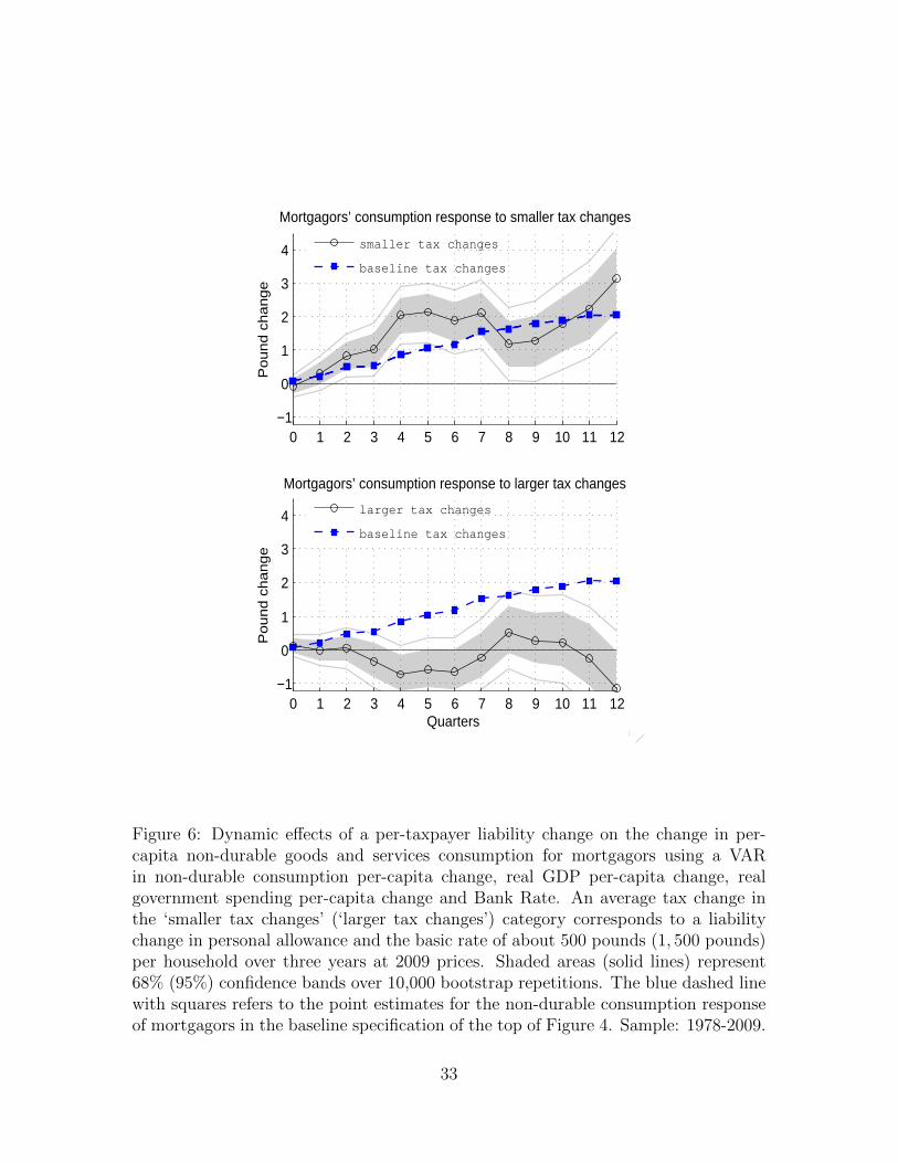
Small versus large tax changes. To verify whether mortgagors are indeed ‘wealthy’

hand-to-mouth as in Kaplan and Violante (2014), Figure 6 shows the response of non-

durable consumption for this tenure group to ‘smaller’ and ‘larger’ tax changes. For

any given quarter, we define a change in our tax change series as ‘smaller’ (‘larger’)

if the associated household income change over the subsequent three years is below

(above) 1, 200 pounds at 2009 prices. While the results below are not specific to this

value, the choice of the 1, 200 pounds cut-off allows us to split our baseline measure

into two groups whose averages are sufficiently far apart, at about 500 pounds and

1, 500 pounds respectively.

A key finding from Figure 6 is that mortgagors significantly adjust their non-

durable consumption only in response to ‘smaller’ tax cuts. The response to ‘larger’

changes, in contrast, is never statistically positive. Furthermore, the difference be-

tween the two dynamic effects is sizable and often significant, especially over the

second year and towards the end of the forecast period. The dashed blue line with

squares repeats the point estimates for mortgagors’ from Figure 4. The comparison

between the blue line with squares and the black lines with circles reveals that the

baseline response is always above the point estimates of the response to the larger

tax changes (as well as outside the associated 95% confidence band) but it is typically

below the point estimates of the response to the smaller tax changes (becoming even

statistically different over part of the second year forecast horizon). In summary, the

size of the income change does appear to trigger different consumption behaviour.20

20We also repeated this exercise for outright owners and social renters, finding little evidence fora significantly different response to the two types of tax changes for these housing tenure groups.

22

An interesting implication of this finding is that, for a ‘wealthy hand-to-mouth’ house-

hold, there may be an optimal tax cut size to stimulate the economy.

Quantitative assessment. To explore further the interpretation of mortgagors as

‘wealthy hand-to-mouth’ households, we compare the magnitude of the cumulated

response of consumption relative to the cumulated response of income implied by our

estimates to the magnitude of the MPCs reported in the partial equilibrium model of

Kaplan and Violante (2014). It is important to note that, however, that the significant

response of income for all housing tenure groups, reported in Appendix E, strongly

suggests that the overall magnitudes of both the consumption and income responses

reflect (at least partially) the general equilibrium effect of the tax cut.

Panel A of Table 2 reports the ratio of the discounted total consumption change

to the total discounted income change triggered by the tax change over the three year

period. Panel B (C), reports the total discounted consumption (income) change over

the three year period relative to the total discounted tax change (about three pounds

in our simulations) simulated over the same period.21,22 For the sake of comparison,

the row labeled Kaplan and Violante (2014) reproduces the quantitative predictions of

their model for hand-to-mouth households (under the column ‘likely mortgagors’) and

non hand-to-mouth households (under the column ‘likely outright owners’) assuming

transactions costs around $1000 (see figure 5(b) in their paper). The rows labeled

Romer and Romer (2010) will be discussed in the next section.

The results in Panel A of Table 2 show that for every pound of additional income,

mortgagors spend a significant fraction on consumption — around 55 pence — across

the three estimation procedures used earlier (based on either predicted probabilities or

actual tenure groups). Interestingly, the confidence bands around the point estimates

for (‘likely’) mortgagors always include the MPC of 0.43 that Kaplan and Violante

21Denoting Xt the annual change of a quarterly variable, the discounted value (relative to the taxchange) over a three year forecast horizon is (βXt+4 + β2Xt+8 + β3Xt+12)/(β + β2 + β3) where thediscount factor is β = 1/(1 + r) with r being the average annual rate of interest.

22The income responses to the tax change reported in Appendix E are based on the VARs ofSection 3, using group-specific income rather than GDP.

23

(2014) report as a plausible value for the wealthy hand-to-mouth households in their

quantitative model. But the same bands never include the MPC of 0.07 for non hand-

to-mouth agents. The response of consumption relative to income for the (‘likely’)

outright owners, in contrast, is never statistically significant and is quantitatively

similar to the MPC of the unconstrained households in Kaplan and Violante (2014).

We conclude that, once the general equilibrium effects are taken into account, our

estimates are consistent with the magnitudes predicted by a quantitative consumption

model where transaction costs make it costly for mortgagor-type households to access

their illiquid asset.

4.3 Comparison with the empirical macro literature

Using a narrative identification approach, a growing body of empirical research in

macroeconomics has estimated the response of aggregate consumption and GDP. For

example, in the seminal contribution by Romer and Romer (2010) the cumulative

multiplier (i.e. the cumulative effect on the variable of interest relative to the size of

the tax change) is around 0.89 for consumption and 1.78 for output.23 Their GDP

multiplier at the peak is around 3. Cloyne (2013) finds similar magnitudes for the

U.K.24 In Panels B and C of Table 2, we compare the findings of this macro literature

with the estimates in our paper (for different household groups using survey micro

data).

In Panel B, the cumulative consumption multiplier is large and significant only

for the (‘likely’) mortgagors. The associated confidence bands also never include

the smaller and insignificant value for the (‘likely’) outright owners. Interestingly,

the estimated response of aggregate Personal Consumption Expenditure (PCE) from

Romer and Romer’s specification sits in-between the set of point estimates for the two

23These numbers refer to the cumulative effect on GDP and consumption replicated using Romers’dataset available online and the exact empirical specifications used in their paper. To make the datamore comparable with our micro data, we use per capita series rather than the aggregate seriescited in the original paper. However, the numbers are very similar when using the non-per capitameasures: 0.88 and 1.61 for consumption and GDP respectively.

24In Cloyne and Surico (2013), we also find similar results for aggregate consumption using officialconsumption data and using an aggregate series constructed from our micro data.

24

tenure groups. Furthermore, the results in Panel C show that the income multiplier

is not quantitatively different between households with debt and households without

debt (with the possible exception of the imprecise point estimates based on actual

housing tenures) and that the implied cumulative multiplier for GDP from Romer

and Romer (2010) appears consistent with the estimates we report for the two groups.

Our findings are therefore consistent with the absolute effects on consumption and

output reported in the empirical macro literature on tax changes.

5 Other explanations

Sections 3 and 4 contain two main messages. First, that the consumption of house-

holds with mortgage debt is the most responsive to changes in taxes. Second, that

our qualitative and quantitative findings are consistent with a model of ‘wealthy hand

to mouth’ consumers.

One may be concerned, however, about a potential selection issue, namely that

mortgage debt is correlated with some other (more structural) trait which makes

households more responsive to tax changes. In this section, we therefore discuss

the extent to which other explanations may fit our findings. Since the behaviour of

social renters seems to square with the predictions of traditional liquidity constraint

models, we focus here on the differential responses of mortgagors and outright owners.

In particular, we will show that demographics, rational inattention, impatience and

risk seem to provide less compelling explanations for all our empirical results. Finally,

we provide further evidence to show that our results are unlikely to be explained by

compositional change.

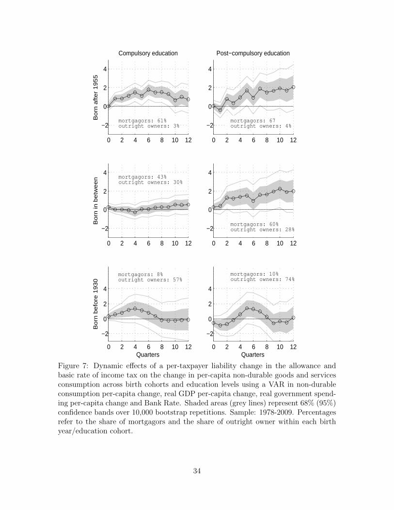
Demographics. A long-standing approach in micro-econometrics has proxied the

presence of liquidity constraints with the household head’s birth year and educational

attainment. However, whether these more traditional dimensions provide sharper

evidence of heterogeneity than housing tenure remains an empirical question and one

25

we tackle in this section.25

The answer provided by Figure 7 is based on VAR specifications in which house-

holds are grouped depending on whether the head is born after 1955 (first row),

between 1930 and 1955 (second row) or before 1930 (third row). The columns then

split these pseudo-cohorts further, depending on whether the household head attained

only compulsory or also post-compulsory education. The point estimates suggest that

the ‘younger’ (born after 1955) and the ‘middled-aged’ more educated tend to change

their non-durable consumption by a larger amount than the other groups. But the

heterogeneity reported in Figure 7 appears more muted and far less precise than the

heterogeneity in Figure 4 where housing tenure was associated with the presence of

liquidity constraints.

Why might grouping by housing tenure deliver clearer evidence of heterogeneity

in the response of consumption?26 To answer this, it is useful to revisit the demo-

graphic statistics in Figure 3. Specifically, we compute the shares of mortgagors and

outright owners within each birth year/education pseudo-cohort. These shares are

also reported in each panel of Figure 7. On the one hand, the largest consumption

responses using the birth year/education split occur for cohorts characterized by the

largest share of mortgagors. On the other hand, in none of the panels in Figure 7

is the share of mortgagors greater than 70%, which potentially explains the larger

confidence intervals relative to Figure 4: each birth year/education pseudo-cohort

pools together households with different debt positions and thus different consump-

tion responses. In Appendix F, we show that similar results and interpretations arise

when we group households by birth year and education separately.27

25A further advantage of grouping households by housing tenure, relative to using birth year,liquidity, leverage or income is that we do not need to take a stand — prior to estimation — on thespecific (and somewhat arbitrary) threshold levels below which a household is considered to be, forexample, younger, poorer or more levered.

26The considerable variation in the rate at which different birth cohorts transition into homeownership reported in Bottazzi et al. (2010) appears another plausible candidate to reconcile theestimates based on the two grouping strategies in Figures 4 and 7.

27In that Appendix, we also show that (i) older mortgagors (born before 1955) still respond morethan older outright owners (also born before 1955), (ii) the response of mortgagors is significant forboth ‘younger’ and ‘older’ cohorts, but (iii) the response of outright owners is never significant.

26

Rational Inattention. An alternative explanation for the mortgagors’ differential

reaction to small and large tax changes might be provided by rational inattention.

To the extent that the ‘smaller’ changes are small relative to household income,

mortgagors may rationally choose to pay little attention to the extra resources and

not re-optimize their consumption-saving plan. On the other hand, as we have already

mentioned, the response of outright home-owners does not vary significantly with the

size of the tax change despite this group having an average income that is only

slightly lower than the mortgagors’. We conclude that rational inattention is unlikely

to explain all our findings.

Impatience and risk aversion. Impatience and risk aversion may play a role in

explaining why mortgagors change their consumption significantly following a tax

change. However, these explanations do not seem to easily explain why mortgagors

respond more to smaller income tax changes than to larger tax changes. As a result,

these hypotheses seem to square less well with our results than housing tenure.

Compositional changes. Even if one can construct a consistent time series of

consumption changes for each cohort (as we have argued in Section 3), a change in the

composition of each tenure group may still affect the interpretation of our estimates.

This could be the case, for instance, if a significant sub-set of social renters took

advantage of the ‘Right-to-Buy’ scheme launched by the Conservative Party during

the 1980s, which allowed those living in accommodation rented from local authorities

or housing associations to purchase their house at a subsidized price.

To explore this compositional change interpretation of our evidence, we perform

two additional exercises. First, in the online Appendix we ask how fast and large such

a compositional change would need to have been to account for the heterogeneity

documented in this paper. The bottom line of this thought-experiment is that it is

very hard to come up with a compositional change that could rationalise the response

of mortgagors without generating predictions for the other groups that are largely at

odds with the rest of our evidence.

27

In the second exercise, we restrict our focus to mortgagors with income above the

median value of their group in each quarter. This sub-set of households with debt is

the most likely to be populated by ‘genuine’ mortgagors (as opposed to social renters

who became mortgagors because of the government incentives). The results in the

Appendix confirms the finding in the top panel of Figure 4, consistent with the view

that compositional changes seem unlikely to account for our findings.

6 Concluding remarks

Recent years have witnessed a renewed interest in the role of household debt in the

transmission of macroeconomic shocks. Theoretical studies have formalised the idea

that some agents may become liquidity constrained by purchasing a large illiquid asset

such as housing. A main implication of this ongoing research effort is that, following

an exogenous change in taxes, households with mortgage debt could increase their

consumption by more than those without.

Our results are strongly suggestive of the notion that tax cuts affect consumption

mostly by relaxing liquidity constraints for indebted households. In particular, we are

able to document that the data line up with a number of qualitative and quantita-

tive predictions of models stressing illiquidity problems faced by households who have

significant positive net wealth. However, because mortgage status is not randomly as-

signed, there are potential selection concerns that imply our analysis may not be fully

conclusive. Identifying, or engineering, an empirical setting where mortgagor versus

outright owner status is randomly assigned appears to be a formidable challenge, but

definitive proof that mortgage status is the cause of households’ response to tax cuts

may have to await for such a feat to be accomplished. Nevertheless, the result that

a household’s debt position is a strong predictor of its consumption response to tax

cuts has potentially far-reaching policy implications.

28

‐1.5

‐1

‐0.5

0

0.5

1

1.5

2

1975 1980 1985 1990 1995 2000 2005 2010

All exogenous tax changes

Exogenous allowance and basic rateincome tax changes

Figure 1: Tax liability changes over GDP: income tax measure (red) vs. all exogenoustax changes (black dashed)

0.0

0.1

0.2

0.3

0.4

0.5

0.6

0.7

0.8

0.9

1.0

Social renters

Mortgagors

Owners outright

Figure 2: Shares of social renters, mortgagors and outright home owners.

29

0.0

1.0

2.0

3.0

4D

ensity

20 40 60 80 100Age of household head

Social renters Mortgagors

Owned outright

Age: 1978-2009

0.2

.4.6

.8F

raction

Proportion with post-compulsory education

Education: 1978-2009

Mortgagors Social rentersOwners outright

0.0

02

.004

.006

.008

.01

Density

0 100 200 300 400 500 600 700 800Weekly real income per adult

Social renters Mortgagors

Owned outright

Weekly real income per adult: 1978-2009

0.1

.2.3

.4.5

Fra

ction

Proportion with loans (FES): 1986-2009

Mortgagors Social rentersOwners outright

Figure 3: Distributions of age and income and proportions of households with post-compulsory education and non-mortgage loans across housing tenures.

30

Response of non−durable consumption: mortgagors

Po

un

d c

ha

ng

e

0 1 2 3 4 5 6 7 8 9 10 11 12−1

0

1

2

3

4

Response of non−durable consumption: social renters

Po

un

d c

ha

ng

e

0 1 2 3 4 5 6 7 8 9 10 11 12−1

0

1

2

3

4

Response of non−durable consumption: outright owners

Quarters

Po

un

d c

ha

ng

e

0 1 2 3 4 5 6 7 8 9 10 11 12−1

0

1

2

3

4

Figure 4: Dynamic effects of a per-taxpayer liability change in the allowance andbasic rate of income tax on the change in per-capita non-durable goods and servicesconsumption across housing tenures using a VAR in non-durable consumption per-capita change, real GDP per-capita change, real government spending per-capitachange and Bank Rate specified as in Section 3. Shaded areas (grey lines) represent68% (95%) confidence bands over 10,000 bootstrap repetitions. Sample: 1978-2009.

31

Likely mortgagors

Pou

nd c

hang

e

0 1 2 3 4 5 6 7 8 9 10 11 12

−1

0

1

2

3

4

Likely outright owners

Pou

nd c

hang

e

0 1 2 3 4 5 6 7 8 9 10 11 12

−1

0

1

2

3

4

Likely mortgagors

Pou

nd c

hang

e0 1 2 3 4 5 6 7 8 9 10 11 12

−1

0

1

2

3

4

Likely outright owners

Pou

nd c

hang

e

0 1 2 3 4 5 6 7 8 9 10 11 12

−1

0

1

2

3

4

Figure 5: Dynamic effects of a per-taxpayer liability change in the allowance andbasic rate of income tax on the change in per-capita non-durable goods and servicesconsumption across predicted housing tenures (based on probit estimation) using aVAR in non-durable consumption per-capita change, real GDP per-capita change, realgovernment spending per-capita change and Bank Rate. Left (right) column refersto full sample (year-by-year) probit and time-varying (fixed) classification cutoff for‘likely’ and ‘unlikely’ mortgagors. Shaded areas (grey lines) represent 68% (95%)confidence bands over 10,000 bootstrap repetitions. Sample: 1978-2009.

32

Po

un

d c

ha

ng

e

Mortgagors’ consumption response to smaller tax changes

0 1 2 3 4 5 6 7 8 9 10 11 12−1

0

1

2

3

4

Quarters

Po

un

d c

ha

ng

e

Mortgagors’ consumption response to larger tax changes

0 1 2 3 4 5 6 7 8 9 10 11 12−1

0

1

2

3

4

smaller tax changes

baseline tax changes

larger tax changes

baseline tax changes

Figure 6: Dynamic effects of a per-taxpayer liability change on the change in per-capita non-durable goods and services consumption for mortgagors using a VARin non-durable consumption per-capita change, real GDP per-capita change, realgovernment spending per-capita change and Bank Rate. An average tax change inthe ‘smaller tax changes’ (‘larger tax changes’) category corresponds to a liabilitychange in personal allowance and the basic rate of about 500 pounds (1, 500 pounds)per household over three years at 2009 prices. Shaded areas (solid lines) represent68% (95%) confidence bands over 10,000 bootstrap repetitions. The blue dashed linewith squares refers to the point estimates for the non-durable consumption responseof mortgagors in the baseline specification of the top of Figure 4. Sample: 1978-2009.

33

Compulsory education

Bo

rn a

fte

r 1

95

5

0 2 4 6 8 10 12

−2

0

2

4

Post−compulsory education

0 2 4 6 8 10 12

−2

0

2

4

Bo

rn in

be

twe

en

0 2 4 6 8 10 12

−2

0

2

4

0 2 4 6 8 10 12

−2

0

2

4

Quarters

Bo

rn b

efo

re 1

93

0

0 2 4 6 8 10 12

−2

0

2

4

Quarters0 2 4 6 8 10 12

−2

0

2

4

mortgagors: 43%outright owners: 30%

mortgagors: 8%outright owners: 57%

mortgagors: 10%outright owners: 74%

mortgagors: 61%outright owners: 3%

mortgagors: 67outright owners: 4%

mortgagors: 60%outright owners: 28%

Figure 7: Dynamic effects of a per-taxpayer liability change in the allowance andbasic rate of income tax on the change in per-capita non-durable goods and servicesconsumption across birth cohorts and education levels using a VAR in non-durableconsumption per-capita change, real GDP per-capita change, real government spend-ing per-capita change and Bank Rate. Shaded areas (grey lines) represent 68% (95%)confidence bands over 10,000 bootstrap repetitions. Sample: 1978-2009. Percentagesrefer to the share of mortgagors and the share of outright owner within each birthyear/education cohort.

34

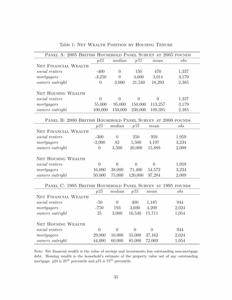
Table 1: Net Wealth Position by Housing Tenure

Panel A: 2005 British Household Panel Survey at 2005 poundsp25 median p75 mean obs

Net Financial Wealthsocial renters -400 0 150 470 1,337mortgagors -3,250 0 4,600 3,014 3,179owners outright 0 3,000 21,540 18,293 2,385

Net Housing Wealthsocial renters 0 0 0 0 1,337mortgagors 55,000 95,000 150,000 113,257 3,179owners outright 100,000 150,000 230,000 189,385 2,385

Panel B: 2000 British Household Panel Survey at 2000 poundsp25 median p75 mean obs

Net Financial Wealthsocial renters -300 0 250 959 1,959mortgagors -2,000 82 5,500 4,197 3,234owners outright 0 3,500 20,000 15,889 2,009

Net Housing Wealthsocial renters 0 0 0 0 1,959mortgagors 16,000 38,000 71,400 54,572 3,234owners outright 50,000 75,000 120,000 97,284 2,009

Panel C: 1995 British Household Panel Survey at 1995 poundsp25 median p75 mean obs

Net Financial Wealthsocial renters -50 0 400 1,185 944mortgagors -750 193 3,690 4,209 2,024owners outright 25 3,000 16,540 15,711 1,054

Net Housing Wealthsocial renters 0 0 0 0 944mortgagors 29,000 10,000 55,000 37,162 2,024owners outright 44,000 60,000 85,000 72,069 1,054

Note: Net financial wealth is the value of savings and investments less outstanding non-mortgage

debt. Housing wealth is the household’s estimate of the property value net of any outstanding

mortgage. p25 is 25th percentile and p75 is 75th percentile.

35

Table 2: Quantitative Comparison with Earlier Contributions

Panel A: consumption relative to income(likely) mortgagors (likely) outright owners

Propensity Score:(time-varying threshold) 0.54∗∗∗

[0.12 , 1.55]0.06

[−0.44 , 0.43]

(fixed threshold) 0.57∗∗∗[0.22 , 1.27]

0.10[−0.75 , 0.66]

Actual Tenure 0.55∗∗∗[0.22 , 1.49]

0.14[−3.58 , 3.55]

Kaplan-Violante 0.43 0.07

Panel B: consumption relative to taxes(likely) mortgagors (likely) outright owners

Propensity Score(time-varying threshold) 1.06∗∗∗

[0.23 , 1.88]0.12

[−0.63 , 0.90]

(fixed threshold) 1.30∗∗∗[0.52 , 2.11]

0.16[−0.64 , 0.98]

Actual Tenure 1.33∗∗∗[0.55 , 2.16]

0.10[−0.62 , 0.87]

Romer-Romer PCE: 0.89

Panel C: income relative to taxes(likely) mortgagors (likely) outright owners

Propensity Score(time-varying threshold) 1.97∗∗∗

[0.62 , 3.33]2.13∗∗∗

[0.87 , 3.40]

(fixed threshold) 2.29∗∗∗[1.08 , 3.53]

1.68∗∗∗[0.38 , 2.98]

Actual Tenure 2.40∗∗∗[0.85 , 3.96]

0.70[−1.00 , 2.50]

Romer-Romer GDP: 1.78

Note: Panel A reports the ratio of the present value of the non-durable expenditure change to thepresent value of the disposable income change in the three years after the shock. Panel B (C)records the ratio of the discounted total non-durable expenditure (disposable income) change tothe discounted total tax change over the same horizon. PCE (GDP) stands for per-capita PersonalConsumption Expenditure (Gross Domestic Product) from National Accounts. The rows for Romerand Romer (2010) refer to the U.S.; similar findings are obtained for the U.K. following Cloyne(2013). Squared brackets display the [5th , 95th] percentiles of the distribution of interest across10,000 bootstrap repetitions. Asterisks denote significance at the 5% level.

36

References

Anderson, E., A. Inoue, and B. Rossi (2012). Heterogeneous consumers and fiscal

policy shocks. mimeo, Duke University, NCSU and UPF .

Andres, J. A., J. E. Bosca, and J. Ferri (2012). Household leverage and fiscal multi-

pliers. Banco de Espana Documentos de Trabajo No. 1215 .

Attanasio, O., J. Banks, and S. Tanner (2002). Asset holding and consumption

volatility. Journal of Political Economy 110, 771–792.

Auerbach, A. and Y. Gorodnichenko (2012). Measuring the output responses to fiscal

policy. American Economic Journal: Economic Policy 4(2), 1–27.

Auerbach, A. and Y. Gorodnichenko (2013). Fiscal multipliers in recession and ex-

pansion. Fiscal Policy after the Financial Crisis NBER chapters, 63–98.

Bottazzi, R., T. Crossley, and M. Wakefield (2010). Late starters or excluded gener-

ations? a cohort analysis of catch up in home ownership in england. Institute for

Fiscal Studies WP 12/10 .

Browning, M., A. Deaton, and M. Irish (1985). A profitable approach to labour

supply and commodity demands over the life-cycle. Econometrica 53(3), 503–44.

Caldara, D. and C. Kamps (2008). What are the effects of fiscal shocks? a var-based

comparative analysis. ECB Working Paper Series 877 .

Caldara, D. and C. Kamps (2012). The analytics of SVARs: A unified framework to

measure fiscal multipliers. FEDS Working Paper 2012-20, Board of Governors of

the Federal Reserve System.

Cloyne, J. and P. Surico (2013). Household debt and the dynamic effects of income

tax changes. CEPR Discussion Paper No. 9649 .

37

Cloyne, J. S. (2012). Discretionary tax shocks in the United Kingdom 1945-2009: a

new narrative account and dataset. http://ideas.repec.org/e/pcl85.html .

Cloyne, J. S. (2013). Discretionary tax changes and the macroeconomy: new narrative

evidence from the United Kingdom. American Economic Review 103(4), 1507–28.

Crossley, T. and C. O’Dea (2010). The wealth and saving of uk families on the eve

of the crisis. Institute for Fiscal Studies .

De Giorgi, G. and L. Gambetti (2012a). Consumption heterogeneity and the effects

of aggregate shocks. mimeo, Stanford and Autonoma de Barcelona.

De Giorgi, G. and L. Gambetti (2012b). The effects of government spending on the

distribution of consumption. mimeo, Stanford and Autonoma de Barcelona.

Dynan, K. (2012). Is a household debt overhang holding back consumption? Brooking

Papers on Economic Activity Spring, 299–362.

Eggertsson, G. and P. Krugman (2012). Debt, deleveraging, and the liquidity trap:

A Fisher-Minsky-Koo approach. Quarterly Journal of Economics 127, 1469–513.

Ercolani, V. and N. Pavoni (2012). The precautionary saving effect of government

consumption. Mimeo, Bank of Portugal and Bocconi University .

Giavazzi, F. and M. McMahon (2012). The household effects of government spending.

in Fiscal Policy after the Financial Crisis, Eds. Alesina, A. and Giavazzi, F.,

University of Chicago Press .

Guajardo, J., D. Leigh, and A. Pescatori (2011). Expansionary austerity: New inter-

national evidence. IMF WP/11/158 .

IMF (2012). Dealing with household debt. Global Economic Outlook Ch. 3, 89–124.

Kaplan, G. and G. L. Violante (2014). A model of the consumption response to fiscal

stimulus payments. Econometrica, 82, 1199–1239.

38

Kaplan, G., G. L. Violante, and J. Weidner (2014). The wealthy hand-to-mouth.

Brookings Papers On Economic Activity, Spring.

Mertens, K. and M. O. Ravn (2012). Empirical evidence on the aggregate effects of

anticipated and unanticipated U.S. tax policy shocks. American Economic Journal:

Economic Policy 4(2), 145–181.

Mertens, K. and M. O. Ravn (2013). The dynamic effects of personal and corporate

income tax changes in the United States. American Economic Review 103(4),

1212–47.

Mian, A., K. Rao, and A. Sufi (2012). Household balance sheets, consumption, and

the economic slump. mimeo, Princeton University and University of Chicago.

Misra, K. and P. Surico (2014). Consumption, income changes and heterogeneity: Ev-

idence from two fiscal stimulus programmes. American Economic Journal: Macro-

conomics, forthcoming.

Mountford, A. and H. Uhlig (2009). What are the effects of fiscal policy shocks.

Journal of Applied Econometrics 24(6), 960–992.

Nekarda, C. and V. Ramey (2011). Industry evidence on the effects of government

spending. American Economic Journal: Macroeconomics 3(1), 36–59.

Owyang, M. T., V. Ramey, and S. Zubairy (2013). Are government spending multi-

pliers greater during periods of slack? evidence from 20th century historical data.

NBER Working Papers 18769 .

Ramey, V. and M. Shapiro (1998). Costly capital reallocation and the effects of

government spending. Carnegie Rochester Series on Public Policy 48, 145–194.

Ramey, V. A. (2011). Identifying government spending shocks: It’s all in the timing.

Quarterly Journal of Economics 126(1), 1–50.

39

Romer, C. D. and D. H. Romer (1989). Does monetary policy matter? A new test

in the spirit of Friedman and Schwartz. NBER Macroeconomic Annual 1989 .

Romer, C. D. and D. H. Romer (2004). A new measure of monetary shocks: Derivation

and implications. American Economic Review 94(4), 1055–84.

Romer, C. D. and D. H. Romer (2010). The macroeconomic effects of tax changes:

Estimates based on a new measure of fiscal shocks. American Economic Re-

view 100(3), 763–801.

40

Appendices

A The UK income tax system

In the United Kingdom, income tax accounts for around 25–30 per cent of total

government revenue and consists of a set of allowances, bands of income and marginal

tax rates that apply to each income band. Each individual has a personal allowance

which is deducted from their income to calculate their ‘taxable income’. An income

taxpayer is therefore someone who earns more than their allowance (although there

is a system of tax credits that lowers the tax liability of the poorest taxpayers). In

the tax year 2012-2013, for instance, the first 34, 370 pounds above the allowance

was subject to a 20 per cent rate, any further earnings up to 150, 000 pounds were

subject to a 40 per cent rate and then 50 per cent was charged on all earnings over

£ 150,000. These bands and allowances are increased each year in line with inflation

unless the UK Parliament decides otherwise. We do not treat automatic inflationary

increases as tax shocks in our data set.

B Data description

B.1 Aggregate data

• GDP and government spending data: UK Office for National Statistics codes

ABMI, BKTL and NMRY. UK Total Population data are from Eurostat. FTSE

data are the FTSE All Share Index from Bloomberg.

• Price index : Retail Prices Index excluding mortgage interest payments (RPIX),

ONS codes CHMK and CDKQ (extended back from 1976 using the growth in

the Retail Prices Index, CZBH).

• We scale our tax measure by the total number of taxpayers, available from Her

Majesty’s Revenue and Customs’ website (www.hmrc.gov.uk).

41

• Data on income tax thresholds used for constructing our final micro dataset are

from the Institute for Fiscal Studies (www.ifs.org.uk). See the text for more

discussion.

• Data sources for the construction of our income tax shocks can be found in the

Online Appendix. The tax series also makes use of tax shock data from Cloyne

(2013).

B.2 Household micro data

We use the Family Expenditure Survey (later called the Expenditure and Food Survey

and, recently, the Living Costs and Food Survey) from 1978 to 2009. These data are

available from the UK Data Archive.

Household consumption expenditure

• Non-durable goods and services expenditure: includes food, alcohol, tobacco,

fuel, light and power, clothing and footwear, personal goods and services, fares,

leisure services, household services, non-durable household goods, motoring ex-

penditures and leisure goods.

• Durable expenditure: durable household goods, motor vehicles and durable

leisure goods. This includes expenditure such as furniture and furnishings,

electrical appliances and audio-visual equipment.

• Total non-housing expenditure: total expenditure minus housing expenditures

(including rents, rates and water charges).

• We gross-up using household weights and divide by the number of household

members to construct a per capita measure.

Housing tenure

The FES records the tenure status of households. Social renters are defined as

those living in local authority housing or accommodation provided by housing associ-

ations. Mortgagors and owners are taken directly from the FES. The private renters

42

category is dropped due to the limited number of observations.

Demographics and other loan

The demographic variables are taken from the FES: age, education and employment

status of the head of household. The data on non-mortgage loans is a binary indicator

for whether the household also has another type of loan other than a mortgage.

British Household Panel Survey

The BHPS is available from the UK Data Archive.

43

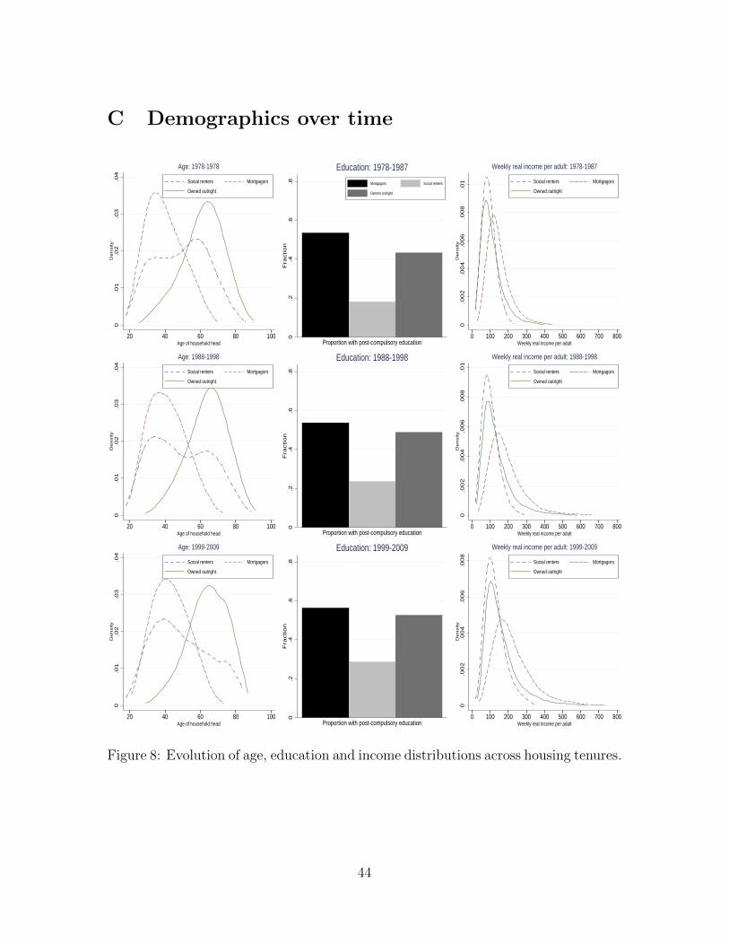
C Demographics over time0

.01

.02

.03

.04

De

nsity

20 40 60 80 100Age of household head

Social renters Mortgagors

Owned outright

Age: 1978-1978

0.2

.4.6

.8F

raction

Proportion with post-compulsory education

Education: 1978-1987

Mortgagors Social renters

Owners outright

0.0

02

.004

.006

.008

.01

De

nsity

0 100 200 300 400 500 600 700 800Weekly real income per adult

Social renters Mortgagors

Owned outright

Weekly real income per adult: 1978-1987

0.0

1.0

2.0

3.0

4D

en

sity

20 40 60 80 100Age of household head

Social renters Mortgagors

Owned outright

Age: 1988-1998

0.2

.4.6

.8F

raction

Proportion with post-compulsory education

Education: 1988-1998

0.0

02

.004

.006

.008

.01

De

nsity

0 100 200 300 400 500 600 700 800Weekly real income per adult

Social renters Mortgagors

Owned outright

Weekly real income per adult: 1988-1998

0.0

1.0

2.0

3.0

4D

en

sity

20 40 60 80 100Age of household head

Social renters Mortgagors

Owned outright

Age: 1999-2009

0.2

.4.6

.8F

raction

Proportion with post-compulsory education

Education: 1999-2009

0.0

02

.004

.006

.008

De

nsity

0 100 200 300 400 500 600 700 800Weekly real income per adult

Social renters Mortgagors

Owned outright

Weekly real income per adult: 1999-2009

Figure 8: Evolution of age, education and income distributions across housing tenures.

44

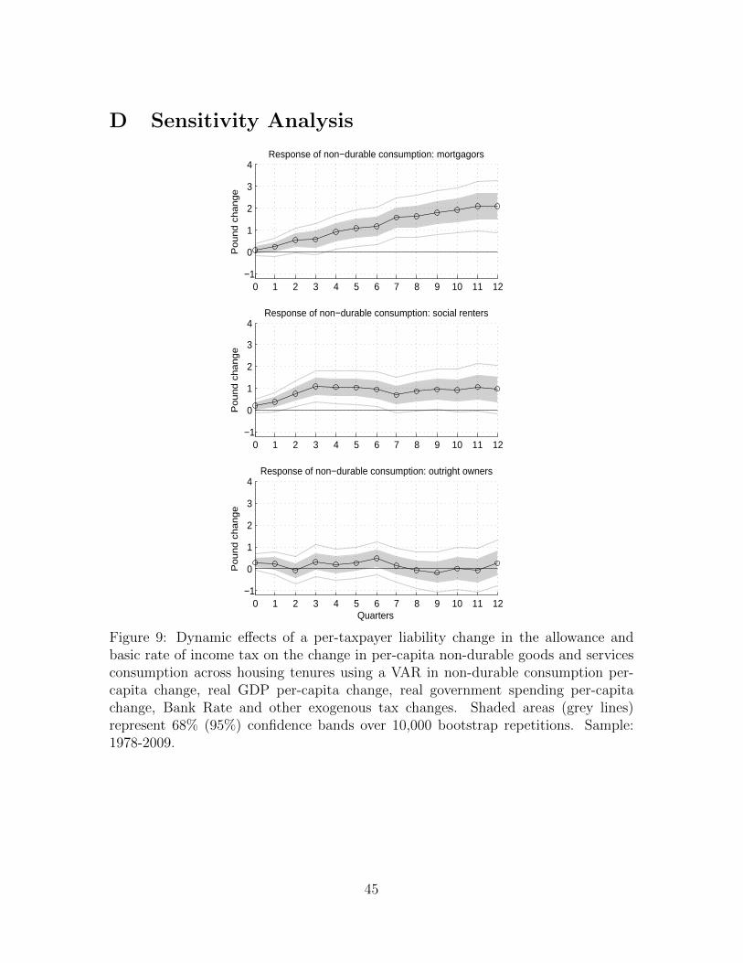
D Sensitivity Analysis

Response of non−durable consumption: mortgagors

Po

un

d c

ha

ng

e

0 1 2 3 4 5 6 7 8 9 10 11 12−1

0

1

2

3

4

Response of non−durable consumption: social renters

Po

un

d c

ha

ng

e

0 1 2 3 4 5 6 7 8 9 10 11 12−1

0

1

2

3

4

Response of non−durable consumption: outright owners

Quarters

Po

un

d c

ha

ng

e

0 1 2 3 4 5 6 7 8 9 10 11 12−1

0

1

2

3

4

Figure 9: Dynamic effects of a per-taxpayer liability change in the allowance andbasic rate of income tax on the change in per-capita non-durable goods and servicesconsumption across housing tenures using a VAR in non-durable consumption per-capita change, real GDP per-capita change, real government spending per-capitachange, Bank Rate and other exogenous tax changes. Shaded areas (grey lines)represent 68% (95%) confidence bands over 10,000 bootstrap repetitions. Sample:1978-2009.

45

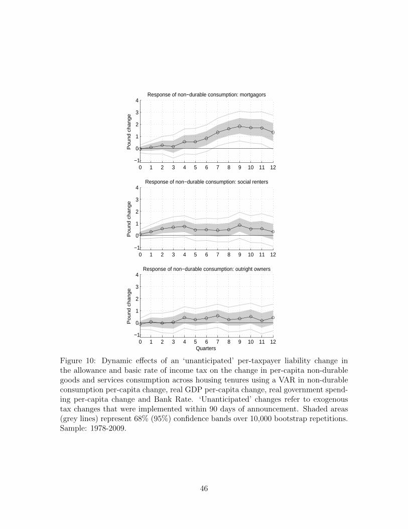
Response of non−durable consumption: mortgagors

Po

un

d c

ha

ng

e

0 1 2 3 4 5 6 7 8 9 10 11 12−1

0

1

2

3

4

Response of non−durable consumption: social renters

Po

un

d c

ha

ng

e

0 1 2 3 4 5 6 7 8 9 10 11 12−1

0

1

2

3

4

Response of non−durable consumption: outright owners

Quarters

Po

un

d c

ha

ng

e

0 1 2 3 4 5 6 7 8 9 10 11 12−1

0

1

2

3

4

Figure 10: Dynamic effects of an ‘unanticipated’ per-taxpayer liability change inthe allowance and basic rate of income tax on the change in per-capita non-durablegoods and services consumption across housing tenures using a VAR in non-durableconsumption per-capita change, real GDP per-capita change, real government spend-ing per-capita change and Bank Rate. ‘Unanticipated’ changes refer to exogenoustax changes that were implemented within 90 days of announcement. Shaded areas(grey lines) represent 68% (95%) confidence bands over 10,000 bootstrap repetitions.Sample: 1978-2009.

46

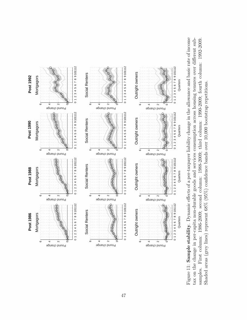
Po

st 1

986

Po

st 1

988

Po

st 1

990

Po

st 1

992

Pound change

Mor

tgag

ors

01

23

45

67

89

1011

12

0246

Pound change

Mor

tgag

ors

01

23

45

67

89

1011

12

0246

Pound change

Mor

tgag

ors

01

23

45

67

89

1011

12

0246

Pound change

Mor

tgag

ors

01

23

45

67

89

1011

12

0246

Pound change

Soc

ial R

ente

rs

01

23

45

67

89

1011

12

0246

Pound change

Soc

ial R

ente

rs

01

23

45

67

89

1011

12

0246

Pound change

Soc

ial R

ente

rs

01

23

45

67

89

1011

12

0246

Pound change

Soc

ial R

ente

rs

01

23

45

67

89

1011

12

0246

Qua

rter

s

Pound change

Out

right

ow

ners

01

23

45

67

89

1011

12

0246

Qua

rter

s

Pound change

Out

right

ow

ners

01

23

45

67

89

1011

12

0246

Qua

rter

s

Pound change

Out

right

ow

ners

01

23

45

67

89

1011

12

0246

Qua

rter

s

Pound change

Out

right

ow

ners

01

23

45

67

89

1011

12

0246

Fig

ure

11:

Sam

ple

stabil

ity

.D

ynam

iceff

ects

ofa

per

-tax

pay

erliab

ilit

ych

ange

inth

eal

low

ance

and

bas

icra

teof

inco

me

tax

onth

ech

ange

inp

er-c

apit

anon

-dura

ble

goods

and

serv

ices

consu

mpti

onac

ross

hou

sing

tenure

sov

erdiff

eren

tsu

b-

sam

ple

s.F

irst

colu

mn:

1986

-200

9;se

cond

colu

mn:

1988

-200

9;th

ird

colu

mn:

1990

-200

9;fo

urt

hco

lum

n:

1992

-200

9.Shad

edar

eas

(gre

ylines

)re

pre

sent

68%

(95%

)co

nfiden

ceban

ds

over

10,0

00b

oot

stra

pre

pet

itio

ns.

47

Food

Mor

tgag

ors

0 2 4 6 8 10 12

0

2

4

Strictly non−durable

0 2 4 6 8 10 12

0

2

4

Non−housing

0 2 4 6 8 10 12

0

2

4

Soc

ial r

ente

rs

0 2 4 6 8 10 12

0

2

4

0 2 4 6 8 10 12

0

2

4

0 2 4 6 8 10 12

0

2

4

Quarters

Out

right

Ow

ners

0 2 4 6 8 10 12

0

2

4

Quarters0 2 4 6 8 10 12

0

2

4

Quarters0 2 4 6 8 10 12

0

2

4

Figure 12: Dynamic effects of a per-taxpayer liability change in the allowance andbasic rate of income tax on the change in per-capita expenditure on food, strictlynon-durable and non-housing goods and services across housing tenures using a VARin non-durable consumption per-capita change, real GDP per-capita change, realgovernment spending per-capita change and Bank Rate. Shaded areas (grey lines)represent 68% (95%) confidence bands over 10,000 bootstrap repetitions. Sample:1978-2009.

48

Response of non−durable consumption: mortgagors

Po

un

d c

ha

ng

e

0 1 2 3 4 5 6 7 8 9 10 11 12−1

0

1

2

3

4

Response of non−durable consumption: social renters

Po

un

d c

ha

ng

e

0 1 2 3 4 5 6 7 8 9 10 11 12−1

0

1

2

3

4

Response of non−durable consumption: outright owners

Quarters

Po

un

d c

ha

ng

e

0 1 2 3 4 5 6 7 8 9 10 11 12−1

0

1

2

3

4

Figure 13: Dynamic effects of a per-taxpayer liability change in the allowance andbasic rate of income tax on the change in per-capita non-durable goods and servicesconsumption across housing tenure using a VAR in non-durable consumption per-capita change, real GDP per-capita change, real government spending per capitachange and Bank Rate, controlling for the amount of the tax change. Shaded areas(grey lines) represent 68% (95%) confidence bands over 10,000 bootstrap repetitions.Sample: 1978-2009.

49

EIn

com

ere

sponse

s

Pro

bit t

ime−

vary

ing

tres

hold

Act

ual h

ousi

ng te

nure

Pro

bit f

ixed

thre

shol

d

Pound change

Mor

tgag

ors

01

23

45

67

89

1011

12−

1012345

Qua

rter

s

Pound change

Out

right

ow

ners

01

23

45

67

89

1011

12−

101234

Pound change

Like

ly m

ortg

agor

01

23

45

67

89

1011

12−

1012345

Qua

rter

s

Pound change

Like

ly o

utrig

ht o

wne

r

01

23

45

67

89

1011

12−

1012345

Pound change

Like

ly m

ortg

agor

01

23

45

67

89

1011

12−

1012345

Qua

rter

s

Pound change

Like

ly o

utrig

ht o

wne

r

01

23

45

67

89

1011

12−

1012345

Fig

ure

14:

Dynam

iceff

ects

ofa

per

-tax

pay

erliab

ilit

ych

ange

inth

eal

low

ance

and

bas

icra

teof

inco

me

tax

onth

ech

ange

inp

er-c

apit

ain

com

eac

ross

hou

sing

tenure

susi

ng

aV

AR

innon

-dura

ble

consu

mpti

onp

er-c

apit

ach

ange

,re

alp

er-c

apit

ain

com

ech

ange

,re

algo

vern

men

tsp

endin

gp

er-c

apit

ach

ange

and

Ban

kR

ate.

Shad

edar

eas

(gre

ylines

)re

pre

sent

68%

(95%

)co

nfiden

ceban

ds

over

10,0

00b

oot

stra

pre

pet

itio

ns.

Sam

ple

:19

78-2

009.

50

F Further results on demographics

Response of non−durable consumption: born after 1955

Po

un

d c

ha

ng

e

0 1 2 3 4 5 6 7 8 9 10 11 12−1

0

1

2

3

4

Response of non−durable consumption: born in between

Po

un

d c

ha

ng

e

0 1 2 3 4 5 6 7 8 9 10 11 12−1

0

1

2

3

4

Response of non−durable consumption: born before 1930

Quarters

Po

un

d c

ha

ng

e

0 1 2 3 4 5 6 7 8 9 10 11 12−1

0

1

2

3

4

Figure 15: Dynamic effects of a per-taxpayer liability change in the allowance andbasic rate of income tax on the change in per-capita non-durable goods and servicesconsumption across birth cohorts. Shaded areas (grey lines) represent 68% (95%)confidence bands over 10,000 bootstrap repetitions. Sample: 1978-2009.

51

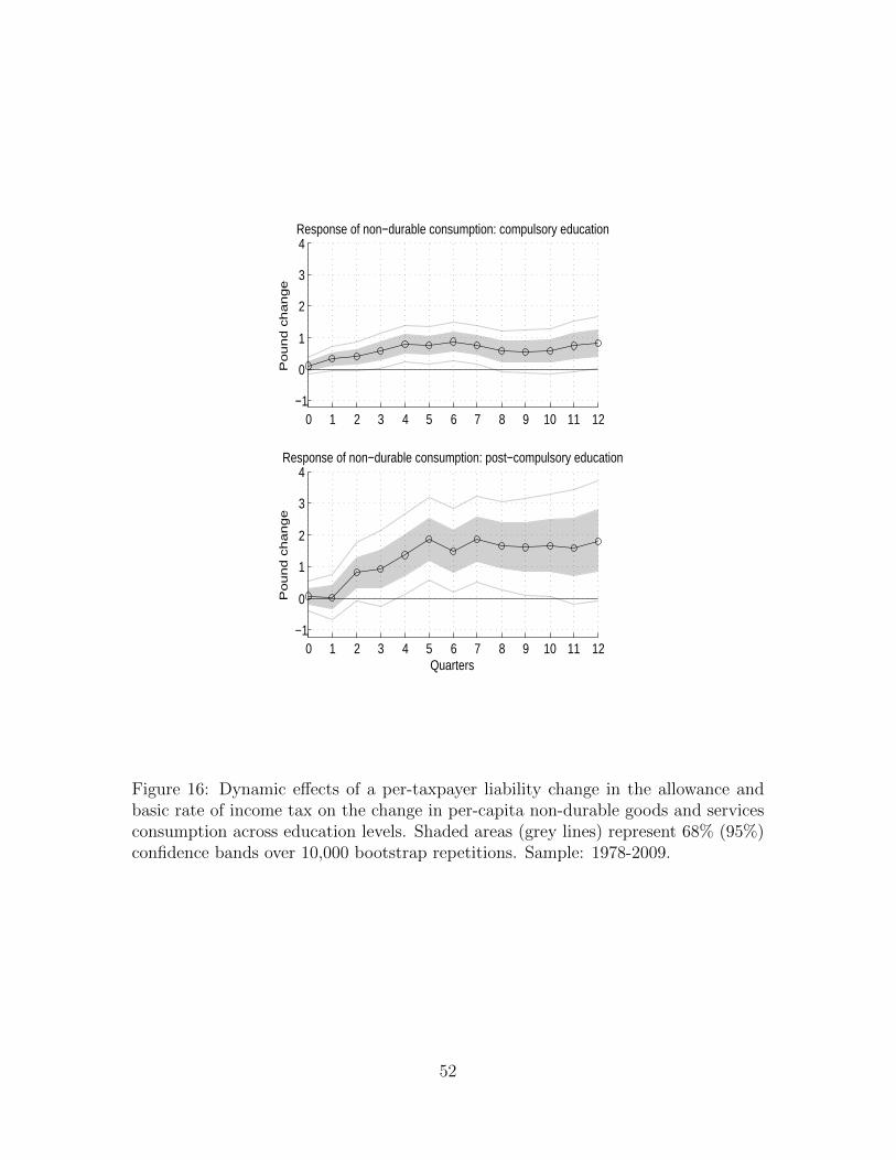
Response of non−durable consumption: compulsory education

Po

un

d c

ha

ng

e

0 1 2 3 4 5 6 7 8 9 10 11 12−1

0

1

2

3

4

Response of non−durable consumption: post−compulsory education

Quarters

Po

un

d c

ha

ng

e

0 1 2 3 4 5 6 7 8 9 10 11 12−1

0

1

2

3

4

Figure 16: Dynamic effects of a per-taxpayer liability change in the allowance andbasic rate of income tax on the change in per-capita non-durable goods and servicesconsumption across education levels. Shaded areas (grey lines) represent 68% (95%)confidence bands over 10,000 bootstrap repetitions. Sample: 1978-2009.

52

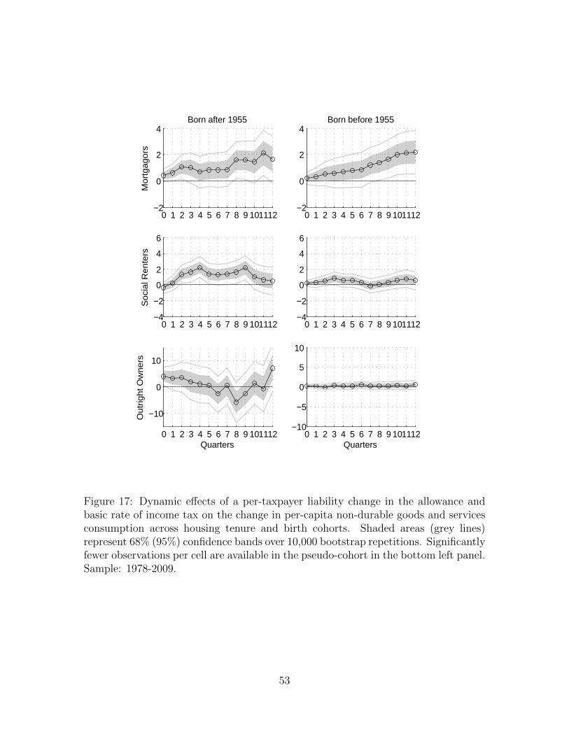
Born after 1955

Mor

tgag

ors

0 1 2 3 4 5 6 7 8 9 101112−2

0

2

4Born before 1955

0 1 2 3 4 5 6 7 8 9 101112−2

0

2

4

Soc

ial R

ente

rs

0 1 2 3 4 5 6 7 8 9 101112−4

−2

0

2

4

6

0 1 2 3 4 5 6 7 8 9 101112−4

−2

0

2

4

6

Out

right

Ow

ners

Quarters0 1 2 3 4 5 6 7 8 9 101112

−10

0

10

Quarters0 1 2 3 4 5 6 7 8 9 101112

−10

−5

0

5

10

Figure 17: Dynamic effects of a per-taxpayer liability change in the allowance andbasic rate of income tax on the change in per-capita non-durable goods and servicesconsumption across housing tenure and birth cohorts. Shaded areas (grey lines)represent 68% (95%) confidence bands over 10,000 bootstrap repetitions. Significantlyfewer observations per cell are available in the pseudo-cohort in the bottom left panel.Sample: 1978-2009.

53

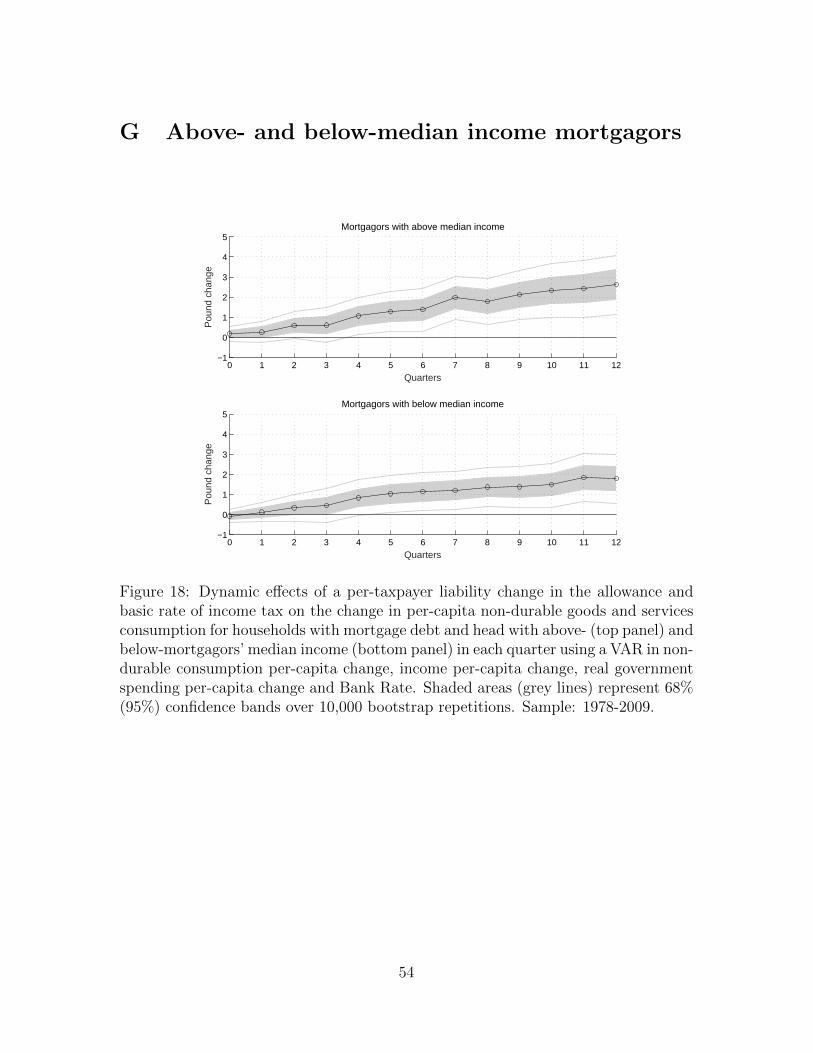
G Above- and below-median income mortgagors

Quarters

Pou

nd c

hang

e

Mortgagors with above median income

0 1 2 3 4 5 6 7 8 9 10 11 12−1

0

1

2

3

4

5

Quarters

Pou

nd c

hang

e

Mortgagors with below median income

0 1 2 3 4 5 6 7 8 9 10 11 12−1

0

1

2

3

4

5

Figure 18: Dynamic effects of a per-taxpayer liability change in the allowance andbasic rate of income tax on the change in per-capita non-durable goods and servicesconsumption for households with mortgage debt and head with above- (top panel) andbelow-mortgagors’ median income (bottom panel) in each quarter using a VAR in non-durable consumption per-capita change, income per-capita change, real governmentspending per-capita change and Bank Rate. Shaded areas (grey lines) represent 68%(95%) confidence bands over 10,000 bootstrap repetitions. Sample: 1978-2009.

54

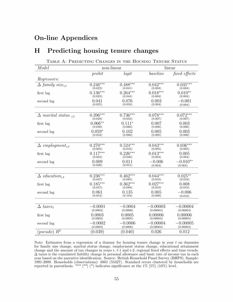
On-line Appendices

H Predicting housing tenure changes

Table A: Predicting Changes in the Housing Tenure Status

Model non-linear linearprobit logit baseline fixed effects

Regressors:∆ family size i,t 0.246∗∗∗

(0.022)0.488∗∗∗(0.041)

0.042∗∗∗(0.004)

0.035∗∗∗(0.004)

first lag 0.136∗∗∗(0.023)

0.264∗∗∗(0.044)

0.018∗∗∗(0.004)

0.010∗∗(0.004)

second lag 0.041(0.025)

0.076(0.050)

0.003(0.004)

−0.001(0.004)

∆ marital status i,t 0.396∗∗∗(0.029)

0.736∗∗∗(0.052)

0.078∗∗∗(0.007)

0.072∗∗∗(0.007)

first lag 0.066∗∗(0.030)

0.111∗(0.066)

0.007(0.006)

0.003(0.006)

second lag 0.059∗(0.034)

0.102(0.066)

0.005(0.005)

0.003(0.006)

∆ employment i,t 0.270∗∗∗(0.005)

0.524∗∗∗(0.045)

0.043∗∗∗(0.005)

0.036∗∗∗(0.005)

first lag 0.117∗∗∗(0.024)

0.226∗∗∗(0.046)

0.013∗∗∗(0.004)

0.005(0.004)

second lag 0.009(0.026)

0.011(0.051)

−0.006(0.004)

−0.010(0.004)

∗∗

∆ education i,t 0.236∗∗∗(0.047)

0.462∗∗∗(0.085)

0.044∗∗∗(0.010)

0.025∗∗(0.010)

first lag 0.185∗∗∗(0.047)

0.362∗∗∗(0.088)

0.027∗∗∗(0.010)

0.008(0.010)

second lag 0.061(0.054)

0.135(0.104)

0.005(0.009)

−0.006(0.010)

∆ taxes t −0.0001(0.0003)

−0.0004(0.0006)

−0.00003(0.00004)

−0.00004(0.00004)

first lag 0.0003(0.0003)

0.0005(0.0005)

0.00006(0.00004)

0.00006(0.00004)

second lag −0.0002(0.0003)

−0.0006(0.0006)

−0.00004(0.00004)

−0.00005(0.00004)

(pseudo) R2 (0.039) (0.040) 0.026 0.012

Note: Estimates from a regression of a dummy for housing tenure change in year t on dummiesfor family size change, marital status change, employment status change, educational attainmentchange and the amount of tax changes in years t, t-1 and t-2, regional fixed effects and time trends.∆ taxes is the cumulated liability change in personal allowance and basic rate of income tax in eachyear based on the narrative identification. Source: British Household Panel Survey (BHPS). Sample:1991-2009. Households (observations): 6801 (55327). Standard errors clustered by households arereported in parenthesis. *** [**] (*) indicates significance at the 1% [5%] (10%) level.

55

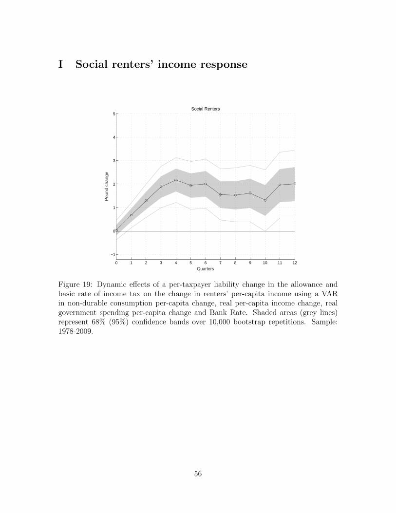
I Social renters’ income response

Quarters

Pou

nd c

hang

eSocial Renters

0 1 2 3 4 5 6 7 8 9 10 11 12

−1

0

1

2

3

4

5

Figure 19: Dynamic effects of a per-taxpayer liability change in the allowance andbasic rate of income tax on the change in renters’ per-capita income using a VARin non-durable consumption per-capita change, real per-capita income change, realgovernment spending per-capita change and Bank Rate. Shaded areas (grey lines)represent 68% (95%) confidence bands over 10,000 bootstrap repetitions. Sample:1978-2009.

56

J Compositional changes: a thought experiment

A further way to assess the interpretation of our results as stemming from mortgagedebt positions rather than the alternative hypothesis of changing group composition,is to ask how large and rapid the transition from one of the other groups to mortgagorswould need to be for the size of our responses to be explained by compositionalchanges.28 For the sake of concreteness, and without loss of generality, considerthe estimated effects for each tenure group at the three year horizon in Figure 4 ofour submission: mortgagors’ response is about 2 pounds, social renters adjust theirconsumption by 1 pound and outright owners make no significant alteration to theirexpenditure. In Figure 2 of this note, we also report that social renters representedroughly 30% (15%) of households at the beginning (end) of the sample, mortgagorsaccounted for another 30% (45%) and outright owners were about 20% (25%). As ourestimates for each group represent average effects over the full sample, it is importantto recognize that the compositional change interpretation of our results relies on thenature of the 15% of population who, over the period 1978-2009, changed housingtenure group to join the mortgagors.

Consider a data generating process in which ‘mortgagors who were never socialrenters’ (which for short we refer to as ‘private mortgagors’) and outright owners are,in fact, all alike in that their expenditure adjustment is statistically indistinguishablefrom zero. This assumption implies that –independently of the speed of transitionbetween tenure groups– the estimated peak effect of 2 pounds for households withdebt in Figure 4 of our submission must be some average of a close-to-zero responseof ‘private’ mortgagors and a higher-than-£2 response of another sub-group, mostlikely within social renters as outright owners exhibit an estimated average responseclose to zero. Similarly, to be consistent with this thought experiment, it must be thecase that the estimated effect of 1 pound for social renters is in fact the average effectover two sub-groups: ‘social renters who became mortgagors’ and ‘social renters whodid not become mortgagors’ (which for short we refer to as ‘long-term social renters’)with the latter having a less-than-£1 response.29

To make the calculations less favorable to our interpretation, we can further as-sume that all switching social renters became mortgagors at the beginning of thesample. As the change of mortgagors share over the full sample is about 15%, thisposes an upper bound to the share of ‘social renters who became mortgagors’ in thepopulation. As 15% is half the share of mortgagors at the beginning of the sampleand ‘private mortgagors’ are assumed not to respond, then it must be the case thatthe peak adjustment of ‘social renters who became mortgagors’ after three years isaround £6, as this value would be consistent with our estimated average responsefor mortgagors of 2 = (2/3) ∗ 0 + (1/3) ∗ 6, where 2/3 is the share of mortgagors atthe beginning of the sample relative to the same share at the end of the sample and1/3 is the assumed share of ‘social renters who became mortgagors’ in the populationover the share of mortgagors at the end of the sample.

It is worth emphasizing two implications of these compositional change calcula-tions. First, notwithstanding the extraordinary large adjustment of £6, the response

28We are grateful to Francesco Caselli for suggesting these calculations.29It is worth noting that the empirical finding of the mortgagors response being higher than the

social renters’ implies that under the compositional change scenario the social renters group needsto be heterogeneous, with some households adjusting their consumption by less than 1 pound (whichis the estimated average response of all social renters) and other households adjusting by more than2 pounds (which is the estimated average response of all mortgagors).

57

of ‘social renters who became mortgagors’ would be inconsistent with the estimatedaverage response of £1 for social renters. The reason is that even assuming that‘long-term social renters’ do not adjust their expenditure at all, the population shareof 15% for ‘social renters who became mortgagors’ vis a vis a population share of35% of social renters at the beginning of the sample implies that the consumptionresponse of the former cannot be larger than £2 to be consistent with an estimatedaverage response of 1 = [(1/2) ∗ 0 + (1/2) ∗ 2].30 Second, assuming any empiricallymore plausible gradualism in the transition from other groups to mortgagors (as op-posed to the abrupt change at the beginning of the sample assumed so far) couldonly make the compositional change interpretation of our results less plausible. Thereason is that under any smooth transition variant of our calculations, the responseof ‘social renters who became mortgagors’ should be further down weighted in theaverage calculations for the mortgagors response to reflect the fraction of the sampleover which the ‘social renters who became mortgagors’ were still part of the socialrenters tenure group.

An alternative way of looking at this second implication of our thought experimentcalculations is to note that if the 15% population share of ‘social renters who becamemortgagors’ switched one third into the sample (rather than at the start of the sampleas assumed in the rest of this section), then their consumption adjustment would needto be 9 pounds for this to be consistent with our estimated effect of £2 for mortgagorsover the full sample (i.e. 2 = {1/3} ∗ 0 + {2/3}[(2/3) ∗ 0 + (1/3) ∗ 9] where the curlybrackets refer to the fractions of the sample period before and after the compositionalchange respectively).

30Note that assuming a ‘private mortgagors’ response of one pound is not sufficient (over andabove being against the spirit of the compositional change interpretation of our results) as ‘socialrenters who became mortgagors’ would still need to adjust their expenditure by 4 pounds, therebystill exceeding the upper limit of £3 that is necessary for their consumption change to be consistentwith an estimated average response for social renters of 2.

58