Finance and Economics Discussion SeriesDivisions of Research & Statistics and Monetary Affairs

Federal Reserve Board, Washington, D.C.

Household Welfare, Precautionary Saving, and Social Insuranceunder Multiple Sources of Risk

Ivan Vidangos

2009-14

NOTE: Staff working papers in the Finance and Economics Discussion Series (FEDS) are preliminarymaterials circulated to stimulate discussion and critical comment. The analysis and conclusions set forthare those of the authors and do not indicate concurrence by other members of the research staff or theBoard of Governors. References in publications to the Finance and Economics Discussion Series (other thanacknowledgement) should be cleared with the author(s) to protect the tentative character of these papers.

Household Welfare, Precautionary Saving, and Social Insurance

under Multiple Sources of Risk�

Ivan Vidangosy

Federal Reserve Board

November 6, 2008

Abstract

This paper assesses the quantitative importance of a number of sources of income risk for

household welfare and precautionary saving. To that end I construct a lifecycle consumption

model in which household income is subject to shocks associated with disability, health, un-

employment, job changes, wages, work hours, and a residual component of household income.

I use PSID data to estimate the key processes that drive and a�ect household income, and

then use the consumption model to: (i) quantify the welfare value to consumers of providing

full, actuarially fair insurance against each source of risk and (ii) measure the contribution of

each type of shock to the accumulation of precautionary savings. I �nd that the value of fully

insuring disability, health, and unemployment shocks is extremely small (well below 1/10 of 1%

of lifetime consumption in the baseline model). The gains from insuring shocks to the wage and

to the residual component of household income are signi�cantly larger (above 1% and 2% of life-

time consumption, respectively). These two shocks account for more than 60% of precautionary

wealth.

�I am indebted to Joe Altonji for his continuous support and encouragement. I would also like to thank TonySmith, Fabian Lange, George Hall, Giuseppe Moscarini, Luigi Pistaferri, Bjoern Bruegemann, Melissa Tartari, andMary Daly for helpful discussions. I am responsible for all remaining shortcomings of the paper. The views expressedhere are my own and do not necessarily represent those of the Board of Governors or the sta� of the Federal ReserveSystem.

yE-mail: ivan.vidangos@frb.gov.

1

1 Introduction

A great deal of attention has been devoted to modeling dynamics and measuring risk in individual

and household income. On one front, there is a substantial empirical literature in labor economics

which has studied the dynamic properties of labor income.1 On a di�erent front, a large number of

studies in macroeconomics and public �nance, which require the speci�cation of an income process

and measures of income uncertainty, have used a variety of strategies to quantify income risk.2

In spite of these large bodies of work, surprisingly little is known about the speci�c sources

underlying income risk and their importance for households' economic well-being. Almost all

existing studies model income risk by means of one or two statistical innovations in a univariate

time-series income process. Such innovations are di�cult to interpret since they capture variation

in income that may be due to a number of rather di�erent factors including unemployment, illness,

job changes, unexpected changes in wages and hours of work, etc. It is impossible to tell from such

formulations which of the many possible sources drive the unexplained variation in income, or what

the relative importance of the di�erent sources is. Yet, identifying the sources of variation and

risk is essential for addressing questions about insurance of risk, since most insurance programs{

whether public or private{typically address speci�c risks, as in the case of unemployment insurance

and disability insurance.

Identifying the various sources of risk and quantifying their e�ects on household welfare ne-

cessitates extending the usual treatment and modeling of income. First, we need to explicitly

account for the fact that households face a large number of risks which are likely to di�er in key

aspects such as their predictability, insurability, relative importance over the lifecycle, etc. Second,

one needs to recognize that households can a�ect their income by adjusting their behavior along a

number of margins, including their labor supply, saving, job-search e�ort, and timing of retirement.

Unfortunately, introducing both multiple risks and multiple choice variables into a decision model

as the one considered here makes the computational cost of solving the model too burdensome.

1This literature includes Lillard and Willis (1978), Lillard and Weiss (1979), Hause (1980), MaCurdy (1982), Halland Mishkin (1982), Abowd and Card (1987, 1989), Topel (1991), Baker (1997), Geweke and Keane (2000), Haider(2001), Meghir and Pistaferri (2004).

2Models that require a measure of income uncertainty or risk have been used to study a wide range of issues,including the following. In macroeconomics: consumption and precautionary saving (Carroll, 1992, 1997; Gourinchasand Parker, 2002; Cagetti, 2003); the distribution of wealth and consumption (Huggett, 1996; Krusell and Smith,1998; Casta~neda, D��az-Gim�enez and R��os-Rull, 2003; Storesletten, Telmer, and Yaron, 2004a); asset pricing (Heatonand Lucas, 1996; Krusell and Smith, 1997; Storesletten, Telmer, and Yaron, 2007). In public �nance: the adequacy ofprivate saving (Engen, Gale, and Uccello, 1999; Scholz, Seshadri, and Khitatrakun, 2006); tax-sheltered accounts andsaving (Engen and Gale, 1993; Engen, Gale, and Scholz, 1994); wealth accumulation (Hubbard, Skinner, and Zeldes,1994, 1995; Dynan, Skinner, and Zeldes, 2004).

2

This paper thus follows most previous studies in treating income as exogenous, and advances the

existing literature by considering a signi�cantly richer speci�cation of income risk.

More speci�cally, I propose a lifecycle consumption model in which households optimally choose

consumption and saving, and where household income is subject to shocks associated with disability,

health, unemployment, job changes, wages, hours, and a residual component of household income.3

The speci�cation allows for complex dynamic relationships which are di�cult to capture in a simple

reduced-form approach. An unemployment shock, for instance, a�ects household income via several

channels: it has a direct negative e�ect on current earnings operating through work hours; it also

has a positive e�ect on household income which re ects both the labor supply response of other

household members as well as unemployment insurance bene�ts; it a�ects the new wage of the

worker upon �nding a new job after the spell of unemployment; and �nally, it a�ects social security

bene�ts during retirement through the e�ect on lifetime average earnings.

I use PSID data to estimate the processes which govern the joint evolution of variables that

drive and a�ect income. Estimation is complicated by the presence of both discrete and continuous

variables, state dependence in several equations, and the need to control for unobserved hetero-

geneity in all equations. I address these issues by using a variety of estimation techniques including

generalized indirect inference.4 The parameterized model is then used to quantify the welfare value

to consumers (in terms of the equivalent variation in lifetime consumption) of providing full, ac-

tuarially fair insurance against each of the sources of uninsured income risk, and to measure the

contribution of each source of uncertainty to the accumulation of precautionary savings.5

Very few previous studies have analyzed the welfare e�ects of multiple sources of risk in a uni�ed

framework. One exception is Low, Meghir, and Pistaferri (2006), who consider a consumption

model with endogenous participation and job-mobility decisions, and two sources of uncertainty:

unemployment and wage risk. They �nd that wage risk has important welfare e�ects but that

unemployment risk does not.

One related line of research has examined a variety of mechanisms to insure household consump-

3I also consider out-of-pocket medical expenditure shocks. However, a proper treatment of these shocks requiresintroducing means-tested transfers, and this complicates the solution of the consumption model signi�cantly. Thecurrent version of the model thus makes the simplifying assumption that medical expenditures can wipe out currentincome but cannot wipe out accumulated wealth, and excludes means-tested transfers. This simpli�es the solutionof the model but it also restricts the potential importance of medical expenditures signi�cantly. Hence, the resultsrelated to medical expenditures are viewed here as very preliminary and are excluded from much of the analysis anddiscussion. A full treatment, including means-tested transfers, is left for future research.

4The implementation of generalized indirect inference in this paper builds on the implementation used in Altonji,Smith, and Vidangos (2008).

5The insurance considered here is additional to already-existing insurance provided by government transfers,self-insurance through saving, and insurance within the family. This will be further discussed below.

3

tion, including unemployment insurance (Gruber, 1997; Browning and Crossley, 2001), food stamps

(Blundell and Pistaferri, 2003), and Medicaid (Gruber and Yelowitz, 1999).6 Some of the empirical

studies in this literature have looked at the e�ects of speci�c income shocks and of speci�c forms

of insurance (such as unemployment and unemployment insurance) on the levels of consumption.

One important di�erence between this paper and those studies is that this paper captures, and

focuses on, the uncertainty in consumption introduced by speci�c sources of income risk, rather

than on the levels of consumption.

My main �ndings are as follows. The welfare gains from fully insuring disability, health, and

unemployment shocks are extremely small (well below 1/10 of 1% of lifetime consumption in the

baseline model). The gains from insuring wage shocks and the additional component of household

income are signi�cantly larger (above 1% and 2% of lifetime consumption, respectively). These

two shocks account for more than 60% of precautionary wealth.

The paper is organized as follows. The next section presents the lifecycle consumption model

and discusses its implementation. Section 3 describes the data. Section 4 presents estimation

results and an evaluation of the �t of the model. Section 5 discusses the solution of the parameter-

ized lifecycle model. Section 6 presents the welfare and precautionary saving analysis, and section

7 concludes.

6Other mechanisms that have been studied include spousal earnings (Cullen and Gruber, 2000; Stephens, 2002),the delay of durable goods purchases (Browning and Crossley, 2001), mortgage re�nancing (Hurst and Sta�ord, 2004),progressive income taxation (Kniesner and Ziliak, 2002), and unsecured debt (Sullivan, 2008).

4

2 Model

2.1 Overview

This section introduces a lifecycle model of consumption in which households face multiple income

shocks. The decision unit is the household and a period corresponds to one year. Households are

part of the labor force for TW years, retire at an exogenously speci�ed date, and live in retirement

for up to TR years.7 Years in the model are indexed by the variable t, where t = 1 indicates the �rst

period of a worker's career. During working years, t thus represents potential experience, although

sometimes t will also be referred to as age, especially when refering to the retirement years. After

retirement, households face mortality risk.

The choice problem facing the household is standard: every period, households choose consump-

tion and saving with the objective of maximizing expected discounted utility over their remaining

periods of life: Et[PTs=t �

s�t�su(cs)], where Et[�] is the expectations operator conditional on infor-

mation available in period t, � � 1 is the discount factor, �t are conditional survival probabilities8,

u is the per-period utility function satisfying u0 > 0, u00 � 0, and limc!0 u0(ct) =1, ct is household

consumption, and T = TW + TR is the maximum age attainable. The household is assumed to

have no bequest motives.

The dynamic budget constraint is zt+1 = (1 + r)(zt � ct) + yt+1, where zt is cash on hand, r is

the real interest rate, and yt+1 is total household nonasset income. Each period, households receive

an exogenous stream of nonasset income yt. During the working years, yt should be thought of

as encompassing all labor and transfer income of the household.9 During the retirement years, yt

consists of social security bene�ts.10 Nonasset income depends on a number of stochastic variables

and shocks: yt+1 = f(st+1; "1;t+1), where "1;t+1 is a vector of shocks and st+1 is a vector of state

variables which describe household characteristics such as health, employment, wage rate, etc.

State variables st evolve stochastically over time according to the law of motion st+1 = g(st; "2;t+1),

where "2;t+1 is a vector of shocks. I next describe separately, and in more detail, the problem faced

by the household in the working years and in the retirement years.

7In implementing the model, TW and TR will be set to 43 and 25, respectively.8Survival probabilities may be allowed to depend not only on age, but also on any other state variable considered

in the model, such as health status.9The appropriate measure of income to use here is after-tax income. The current version of the model does not

distinguish between pre-tax and after-tax income. Future versions will make this distinction, and use after-tax income,by introducing estimated tax functions that approximate e�ective income taxes. Such tax functions are estimated,for instance, by Gouveia and Strauss (1994, 2000) for the years 1966-1989.10One could also allow yt to include a de�ned bene�t pension.

5

2.2 Working Years

During the household's working years, the state variables that a�ect income and are included in

vector st are: (i) an indicator of disability Dt; (ii) an indicator of other health limitations Ht; (iii) an

indicator of employment status Et; (iv) a persistent component of the wage pwt ; and (v) a persistent

component of household income pyt , which captures all residual variation in household income not

explained by earnings of the head or state variables Dt, Ht, and Et. This residual component turns

out to play a large role in explaining the variation of household income in the PSID.11 Households

in the model take into account their current health status, employment status, and non-transitory

aspects of wages and household income when forming expectations about uncertain future nonasset

income.

The household's decision problem during the working years is:

Maximize

Et[TXs=t

�s�t�su(cs)]

subject to

Dt+1 = gD(t;Dt;Ht; "Dt+1; �) (1)

Ht+1 = gH(t;Dt+1; Dt;Ht; "Ht+1; �) (2)

Et+1 = gE(t;Dt+1;Ht+1; Et; "EEt+1; "

UEt+1; "

DEt+1; �) (3)

pwt+1 = gw(Et+1; Et; pwt ; "

wt+1; "

Jt+1; �) (4)

pyt+1 = gy(pyt ; "

yt+1; �) (5)

zt+1 = (1 + r)(zt � ct) + yt+1(t;Dt+1;Ht+1; Et+1; pwt+1; pyt+1; "

Jt+1; "

ht+1; �) (6)

ct � 0; (zt � ct) � �b

Above, equation (1) describes the evolution of the indicator of disability Dt+1. The value of

Dt+1 depends on age t, on whether the household (head) was disabled in the previous period Dt,

on any other previous-period health limitations Ht, and on an iid shock "Dt+1. Index � indicates a

11After accounting for variation in household income due to earnings of the head, household size and composition(including variables that might a�ect the labor supply of a spouse, such as number of children under 6), a polynomialin age, education, race, year indicators, disability, health, employment, and permanent heterogeneity the residual thatremains in household income is large and persistent. This component is represented by pyt and is modeled here as anAR(1) process. This component consists primarily of unexplained variation in spousal labor earnings and transfersfrom public programs.

6

speci�c household type.12 Equation (2) describes the evolution of the health limitations indicator

Ht+1, which depends on age, lagged disability, lagged health, and an iid shock "Ht+1. In addition,

Ht+1 depends on current disability, since Ht+1 is de�ned to be 1 whenever Dt+1 equals 1. Equation

(3) describes the evolution of employment status Et+1, which depends on potential experience t,

current disability status, current health limitations, previous-period employment status, and a set

of iid shocks.13

Equation (4) determines the evolution of the persistent wage component pwt+1, which depends

on current and previous-period employment status (i.e., on the employment transition between the

two periods), on its own lagged value, on an iid shock "wt+1, and on whether there was a job change

between periods t and t�1.14 Equation (5) shows the dependence of the persistent component pyt+1on its own lagged value and a stochastic shock. Equation (6) describes the evolution of cash on

hand, making explicit that the value of household nonasset income yt+1 depends on the realizations

of variables t, Dt+1, Ht+1, Et+1, pwt+1, p

yt+1, "

Jt+1, and "

ht+1.

15 Finally, households cannot borrow

more than amount b in any given period.

2.3 Retirement Years

In all periods following retirement labor income is zero. Retired households receive nonasset

income from social security only. The level of social security bene�ts, SSt+1, is determined in the

last year of work, according to the formula

SSt+1 = PIA(ALE(Dt;Ht; Et; pwt ; p

yt )); (7)

where PIA stands for principal insurance amount and ALE stands for average lifetime earnings.

In the last working year, state variables Dt, Ht, Et, pwt , and p

yt are used to predict average lifetime

earnings. Predicted ALE are then used, along with the rules of the Social Security Administration,

to determine the PIA. Households are assumed to receive a level of bene�ts equal to their PIA.

Details of the calculation of both ALE and PIA are given in Appendix 2. Once the level of social

security bene�ts has been determined, it is assumed to stay constant for as long as the household is

12Types can be de�ned according to permanent observed characteristics (such as education and race) or unobservedcharacteristics (such as unobserved permanent heterogeneity in ability or preferences). The baseline model will beevaluated for one speci�c household type, which will be de�ned below.13These three shocks will determine the transition into employment from three possible states in the previous

period: employment, unemployment, and disability.14Shock "Jt+1 is a job-change shock. Section 4 discusses how job changes are determined.15Some of these variables, in turn, depend on the shocks "Dt+1, "

Ht+1, "

EEt+1, "

UEt+1, "

DEt+1, "

wt+1, and "

yt+1.

7

alive.16 Households also receive asset income, which is determined endogenously within the model.

Retired households in the model may additionally face out-of-pocket medical expendituresMt+1,

which reduce net income disposable for consumption. The household's decision problem during

the retirement years is thus:

Maximize

Et[TXs=t

�s�t�su(cs)]

subject to

Ht+1 = gH(t;Dt+1; Dt;Ht; "Ht+1; �) (2)

pMt+1 = gM (pMt ; "

Mt+1; �) (8)

SSt+1 = gS(SSt) (9)

zt+1 = (1 + r)(zt � ct) + SSt+1 �Mt+1(t;Ht+1; pMt+1) + It+1 (10)

Above, equation (8) describes the evolution of pMt+1, the persistent component of out-of-pocket

medical expenditures. Equation (9) describes the evolution of social security bene�ts. Finally,

equation (10) describes the evolution of cash on hand during retirement, re ecting the fact that

exogenous nonasset income now comes from social security bene�ts SSt+1 and that there may

be out-of-pocket medical expenses Mt+1 which would reduce income available for consumption.

Additionally, households may receive insurance transfers It+1.

Transfers for retired households are intended to provide a minimum level of consumption after

accounting for medical expenditures. These transfers capture the combined e�ects of programs

such as Food Stamps, Supplemental Security Income, and Medicaid. A common speci�cation for

such transfers is It+1 = maxf0;c�+Mt+1 � [SSt+1 + (1 + r)(zt � ct)]g (see Hubbard, Skinner, and

Zeldes (1994, 1995) and Scholz, Seshadri, and Khitatrakun (2006)). The introduction of medical

expenditures and transfers It+1, however, complicates the solution of the consumption decisions

because they introduce nonconvexities which lead to the existence of multiple local maxima in the

solution of the Bellman equation. This problem can be addressed by using a global search in the

optimization involved in the solution of the Bellman equation as in Hubbard, Skinner, and Zeldes

(1994, 1995), but it increases the computation time required to solve the problem signi�cantly.

16In the current version of the model, yt during retirement is calibrated using only social security bene�ts of thehousehold head. A later section discusses how this might a�ect the analysis and results presented here.

8

This will be left for future research. This version makes the simplifying assumption that medical

expenditures can wipe out current income but cannot a�ect accumulated wealth. This assumption

preserves the concavity of the righ-hand-side of the Bellman equation and guarantees that the

unique local maximum is also the global maximum. It also preserves the monotonicity (in wealth)

of the consumption policy functions. On the other hand, this simplifying assumption signi�cantly

restricts the potential importance of medical expenditures. The treatment of medical expenditures

here is thus preliminary and the results should be interpreted with caution. Several studies suggest

that medical expenditures are important for saving behavior and potentially for welfare. Examples

include Palumbo (1999) and De Nardi, French, and Jones (2006).

2.4 Model Implementation

This section discusses two points about implementing the model presented above. The �rst point

regards index � . As mentioned earlier, � indexes the household type. Types can be de�ned based

on observed characteristics (education, race) and unobserved characteristics (unobserved perma-

nent heterogeneity). Di�erent household types will face di�erent processes (di�erent parameter

values) governing the evolution of the various state variables and income. The parameterized

lifecycle model will be evaluated here for one speci�c household type: households whose head is

white, who have the mean level of education in the PSID sample, and who are at the mean of the

distribution of the unobserved permanent heterogeneity components. One important assumption

maintained throughout the analysis is that unobserved heterogeneity is known at the beginning

of a worker's career. Under this assumption, these permanent components do not constitute risk

(i.e., uncertainty).

The second point regards the de�nition of the state variables in the model and their correspon-

dence to variables in the PSID. Most of the variables included in the state vector, such as those

refering to health or employment, will refer to characteristics of the household head in the PSID.

The reason is that these variables are likely to be the most important determinants and predictors

of income. Household income, on the other hand, will refer to a household aggregate in the PSID

which includes labor income and transfer income from all members of the household. I use this

variable to construct predicted income for a household of the average size and composition in the

PSID sample. The household income process is estimated using this predicted income measure

(which has been purged from variation due to di�erences in household size and composition).

9

2.5 Model Parameterization

All parameters that appear in the parameterized form of transition equations (1) - (5) and (8) are

estimated using PSID data. Estimation is discussed in section 4. On the other hand, model

parameters such as the coe�cient or relative risk aversion, the real interest rate, and the discount

factor are chosen based on values found elsewhere in the literature. The sensitivity of results to

alternative assumptions about these parameters is examined in a later section.

Preferences are assumed to be of the constant relative risk aversion (CRRA) form, u(ct) =

c1��t �11�� , where � is the coe�cient of relative risk aversion. The baseline model assumes a value

of � = 3:0.17 The interest rate is assumed to be �xed at the value r = 0:0344 (Gourinchas and

Parker, 2002). The discount factor � is set such that the discount rate equals the interest rate, as

in Low, Meghir, and Pistaferri (2006) and many other studies.18 Conditional survival probabilities

are obtained from the Life Tables published by the Center for Disease and Control Prevention of

the U.S. Department of Health and Human Services. Finally, households in the baseline model

are assumed to be credit-constrained (b = 0).

3 Data

Estimation is conducted using data from the PSID. I start here by giving a brief description of the

key variables. Appendix 1 provides a detailed explanation of all variables used. The disability

indicator Dt equals 1 if an individual is disabled and 0 otherwise. It is constructed from the

respondent's self-reported employment status at the survey date, where \disabled" is one of the

possible answers in the questionnaire. A currently disabled individual is by de�nition not currently

employed. This variable is thus likely to capture severe forms of disability. Indicator Ht, on the

other hand, is constructed based on the survey question: \Do you have any physical or nervous

condition that limits the type of work or the amount of work you can do?" Ht equals 1 when a

respondent answers \yes", and 0 otherwise. This variable is thus likely to capture both serious and

less serious health limitations, including temporary illness and other conditions that a�ect work.

Additionally, Ht is set to 1 whenever Dt equals 1. Employment Et, like disability, is based on

self-reported employment status at the survey date. It equals 1 for employed and temporarily

17The range of values usually considered empirically plausible is 0:5� 5:0. Gourinchas and Parker (2002) estimate� to be around 0:5 � 1:4 in a lifecycle consumption model. Cagetti (2003) obtains considerably higher estimates,around 4:0. Chetty (2006), using a model with consumption and leisure in the utility function, estimates � to bearound 1:0 and argues that values of � above 2:0 are inconsistent with the evidence on labor supply behavior.18Notice that models with �nite horizon do not face the restrictions on the relative values of the discount factor and

the real interest rate that in�nite horizon models have. Smaller values of the discount factor (greater impatience),however, will lead to less saving.

10

laido� workers, and zero for disabled and unemployed individuals. Finally, household income yt

includes all labor and transfer income of the household head and, if present, of the spouse and

any other family members. As was discussed in the previous section, I construct and use predicted

income for a household of the average size and composition in the PSID sample, in order to account

for heterogeneity in household size and composition which is not present in the consumpion model.

As will be discussed below, estimation is conducted in four parts, where each of the following four

subsets of equations is estimated separately: (i) disability; (ii) health; (iii) employment, wage, and

household income; (iv) medical expenditures. Some sample restrictions imposed vary slightly across

the di�erent estimation samples. Estimation of all equations other than medical expenditures uses

data from the 1975-1997 PSID waves. Medical expenditures, on the other hand, use the 1999,

2001, and 2003 waves. The reason is that earlier waves did not contain information on medical

expenses (note also that interviews have been conducted only every two years since 1997).

In all cases, the data include members of both the SRC and SEO samples, as well as nonsample

members who married PSID sample members. I consider only households with a male head

who is living in the household at the time of the interview. Both single and married individuals

are included. I exclude a small fraction of person-year observations in which the head reports

being a full-time student or \keeping house" at the time of the interview. These observations are

discarded because in the lifecycle model household heads cannot be out of the labor force except

when disabled. I also exclude individuals who are missing data on education. Only observations

where the head is at least 18 years old are used.

Some additional sample restrictions, including restrictions based on potential experience (or

age) di�er according to the process being estimated. For estimation of the health limitations

process, I use observations where potential experience ranges from 1 to 65. The corresponding

age range is 18 to 87. This sample has 87; 979 observations. Table 1A (bottom panel) displays

the number of observations and the mean of the health limitations indicator for di�erent levels of

potential experience. The column labeled All t refers to all levels of potential experience, while the

next columns report values for the ranges of potential experience indicated in the top row. The

overall mean of the H indicator is 0:136 and increases from 0:052 for low experience (1 � t � 10)

to 0:497 for high experience (61 < t < 65).

Estimation of disability and of the joint process of employment, wage, and household income

excludes retired individuals and observations where age exceeds 64 (the resulting range of potential

experience is 1 � 48, with very few values above 45. Table 1A (top panel) displays the number

11

of observations and the mean of the disability indicator for di�erent levels of potential experience.

The overall mean of the D indicator is 0:022 and increases from 0:022 for 1 � t � 10 to 0:110 for

t � 41.

In addition, for estimation of the employment, wage, and household income equations (which

also uses data on work hours and labor earnings, as will be discussed below), I censor reported

work hours at 4000, add 200 to reported hours before taking logs to reduce the impact of very low

values on the variation in the logarithm, and I restrict observed wage rates and household income

(in levels) to increase by no more than 500% and decrease to no less than 20% of their previous-

year values.19 I also censor the wage to be no less than $3.50/hour and household income to be no

less than $1,000/year in year-2000 dollars.20 Table 1B displays the number of observations, mean,

standard deviation, minimum, and maximum values of all key variables used in the estimation of

the joint model of income. The second-to-last row displays the raw household income data, while

the last row displays the predicted value for a household of the average size and composition, which

is the variable actually used in estimation.

Finally, estimation of the out-of-pocket medical expenditures process uses observations where

potential experience is above 43, in correspondence with the model's assumption that medical costs

are zero during working years. The PSID variable used here consists of all out-of-pocket payments

made by the household over the course of the two years prior to the interview year (see Appendix

1). Table 1C provides summary statistics in thousands of year-2000 dollars. The sample consists

of 2,831 observations and has a mean of 3:25, a standard deviation of 10:76, a 99th percentile of

38:63, and a maximum value of 317:47.

4 Parameter Estimation

This section presents the parametric models speci�ed for the various transition equations introduced

in section 2 and discusses their estimation. As was mentioned above, the estimation strategy

involves estimating the various equations of the model in four parts. Speci�cally, the equations for

medical expenditures, health limitations, and disability are estimated separately from the rest of

the equations (employment, wage rates, and household income). The reasons for estimating these

equations separately are the following: (i) Out-of-Pocket Medical Expenditures: As discussed above,

19Increases above 500% and declines to less than 20% of the previous value are very uncommon and are likely torepresent reporting errors in most cases.20Given the existence of minimum-wage legislation, reported hourly wages below $3.50/hour are likely to be mis-

reports. Similarly, for a measure of household income as broad as the one used here, very low values of householdincome are likely to be misreports.

12

estimation of medical expenditures uses PSID waves 1999, 2001, and 2003, while all other equations

use data from waves 1975-1997. (ii) Health: In the lifecycle model, health appears as a state

variable both before and after retirement. Estimation of the health process is therefore based on a

sample which includes all levels of potential experience (and age). Most other state variables in the

consumption model (including disability) relate to the labor market and their estimation therefore

excludes high levels of potential experience (and age). (iii) Disability: I initially attempted to

estimate the disability process jointly with all other labor market and income processes. However,

the fact that the disability indicator in the PSID sample is zero more than 97% of the time introduces

numerical instabilities in the implementation of indirect inference.21 Estimating the disability

equation individually allows the use of standard maximum likelihood methods and sidesteps the

numerical di�culties. The following subsections introduce the parametric forms used and discuss

estimation as well as estimation results.

4.1 Disability

The transition equation for the disability indicator Dt is assumed to have the following form

Dt+1 = I[ D0 +

D1 (t+ 1) +

D2 (t+ 1)

2 + D3 (t+ 1)3 + D4 Dt +

D5 Ht + �

D + "Dt+1 > 0]; (11)

where �D is an individual-speci�c, permanent component. In estimation, it is assumed that

�D � N(0; �2�D) and "Dt+1 � N(0; 1) so equation (11) is a dynamic probit with permanent unobserved

heterogeneity. The parameters of equation (11) are estimated by maximum likelihood. The

unobserved component �D is integrated out of the (conditional) likelihood function by Gauss-

Hermite quadrature. The initial condition for Dt is assumed to be zero, since in the PSID sample

Dt = 0 for all individuals for t = 1.

Table 2A presents estimation results for equation (11). The probability that Dt+1 = 1 is

monotonically increasing in experience (the slope of the polynomial is positive for t between 1 and

40). The coe�cient of D4 = 1:611 on Dt indicates a fairly high degree of state dependence.22

Unobserved heterogeneity, with an estimated standard deviation of ��D = 0:934, also plays a

signi�cant role.

21See discussion of estimation mechanics in Appendix 4. The introduction of disability leads to at regions nearthe global optimum of the objective function.22To get a sense of the magnitude of this coe�cient, note that the transitory shock "Dt+1 in the equation has a

standard deviation of 1.

13

4.2 Health

The transition equation for the health indicator is assumed to take the form

Ht+1 = I[ H0 +

H1 (t+ 1) +

H2 (t+ 1)

2 + H3 (t+ 1)3 + H4 Ht + �

H + "Ht+1 > 0]; (12)

where �H is an individual-speci�c permanent component.23 In addition, Ht+1 is set to 1 whenever

Dt+1 equals 1.24 The parameters of equation (12) are also estimated by maximum likelihood, where

�H is assumed to be � N(0; �2�H) and is integrated out of the conditional likelihood by numerical

quadrature. The equation is estimated on the sample of observations where Dt+1 6= 1 (since Ht+1is de�ned to be 1 whenever Dt+1 equals 1). The initial realization of Ht+1 is assumed to be

independent of �H 25, but the distribution of H1 in the model is set such that its mean equals the

mean of H1 in the PSID.

Table 2B presents estimation results (which are conditional on an individual not being disabled).

The probability that Ht+1 = 1 increases monotonically with age. Lagged health limitations

have a fairly large and strongly signi�cant e�ect on the probability of current health limitations

( H4 = 1:119). Unobserved heterogeneity also plays an important role (��H = 0:961).

4.3 Employment, Wage Rates, and Household Income

Employment, wage rates, and household income are determined jointly by a set of recursive equa-

tions. The system also includes an equation for job changes and an equation for work hours.

Although job changes and work hours are not state variables in the lifecycle model, they are key

variables in the determination of income. Therefore, the lifecycle model includes two shocks which

capture job changes and innovations in work hours, respectively. The evolution of job changes and

hours, and their e�ects on income, are thus estimated as part of the recursive system that drives

household income. The following subsection presents the joint model of employment, job changes,

wage rates, work hours, and household income. Additional details are provided in Appendix 3.

23Since the equations for Dt and Ht are estimated separately, I do not estimate the correlation between �D and �H .

This is of no consequence here, however, since I consider households at the mean of the distribution of the variouspermanent heterogeneity components, which is normalized to zero. The important issue is to control for variationdue to permanent components, both because this variation should not represent risk and to avoid bias in coe�cientson lagged dependent variables.24The equation can thus be expressed as Ht+1 = Dt+1 + (1�Dt+1) � I[ H0 + H1 (t+1)+ H2 (t+1)2 + H3 (t+1)3 +

H4 Ht + �H + "Ht+1 > 0].

25Methods that deal with the initial-conditions problem such as that proposed in Wooldridge (2005) are notapplicable here because of the highly unbalanced nature of the sample. I experimented with correcting for initialconditions using the method suggested in Heckman (1981), but the reduced-form approximation of the initial value ofthe latent variable invariably showed very little explanatory power, and hence was not helpful. All dynamic equationsother than equation (12), however, deal with the initial-conditions problem (see Appendix 3).

14

4.3.1 Functional Forms

Employment - Employment Transition

Conditional on being employed, next-period employment is determined by

Et+1 = I[ EE0 + EE1 t+ EE2 t2 + EE3 Ht+1 +

EE4 EDt + �

EE + "EEt+1 > 0]: (13)

Employment-employment transitions are thus determined by a latent variable which depends on

a quadratic polynomial in potential experience t, current health limitations Ht+1, employment

duration EDt, and the error term �EE+"EEt+1. The de�nition of EDt and its treatment is discussed

below. The error component �EE is an individual-speci�c permanent component and "EEt+1 is an iid

idiosyncratic shock. It is assumed that �EE � N(0; �2�EE

) and "EEt+1 � N(0; 1). Component �EE

is allowed to be correlated with unobserved permanent components in the other equations. The

factor structure of the permanent components in the di�erent equations is also speci�ed below.

Unemployment - Employment Transition

Conditional on being unemployed, next-period employment is given by

Et+1 = I[ UE0 + UE1 t+ UE2 t2 + UE3 Ht+1 +

UE4 UDt + �

UE + "UEt+1 > 0]: (14)

Transitions from unemployment into employment are thus determined by a latent variable which

depends on a quadratic polynomial in potential experience t, current health limitations Ht+1,

unemployment duration UDt (discussed below), an individual-speci�c permanent component �UE ,

and the iid idiosyncratic shock "UEt+1 � N(0; 1). The term �UE is assumed to be � N(0; �2�UE

) and

may be correlated with the permanent components in the other equations.

Disability - Employment Transition

Transitions from disability back into employment are rather infrequent in the PSID sample.

These transitions are modeled as

Et+1 = I[ DE0 + "DEt+1 > 0] where "DEt+1 � N(0; 1). (15)

The fact that these transitions are infrequent in the data makes it di�cult to estimate their depen-

dence on experience or on permanent unobserved components.

15

Job Changes

Conditional on being employed in both t and t+1, the occurrence of a job change between the

two periods is determined by

Jt+1 = I[ J0 +

J1 t+

J2 t2 + J3JDt + �

J + "Jt+1 > 0]; (16)

where JDt is job duration (discussed in the next paragraph), �J � N(0; �2

�J) is an individual-speci�c

permanent component, and "Jt+1 � N(0; 1) is iid.

Employment-, Unemployment-, and Job Duration

Estimation of equations (13), (14), and (16) controls for duration dependence in employment

and job mobility by including the variables EDt, UDt, and JDt, respectively. Here, EDt is

de�ned as the number of consecutive periods that an employed individual has been employed up

to period t, UDt is the number of consecutive periods that an unemployed individual has been

unemployed up to period t, and JDt is the number of periods that an employed individual has

been at their current job. It would be straightforward to introduce EDt, UDt, and JDt as state

variables in the lifecycle consumption model from section 2. This is not done here because of

the computational burden of the additional state variables. Instead, the approach is to control

for duration dependence in estimation, but to set the duration variables to their sample mean (by

year of potential experience) when parameterizing the employment and job-change equations. I

also experimented with estimating equations (13), (14), and (16) without controlling for duration

dependence. In this case the potential-experience pro�les of the transition probabilities do not

match the data well, but the results for welfare and precautionary saving are not a�ected.

Wage Equation26

Log wages are assumed to follow the process

lnwaget+1 = �wXw

t+1 + wt+1;

26The speci�cation of the wage process proposed here is similar to one of the speci�cations studied in Altonji,Smith, and Vidangos (2008). A more detailed description of the process is provided in that paper. That paperalso studies alternative speci�cations of the wage process which include job-speci�c components. The reason thatspeci�cations with job-speci�c wage components are not used in this paper is that the job-speci�c wage componentwould introduce an additional state variable in the consumption model, adding to the computational requirementsof its solution.

16

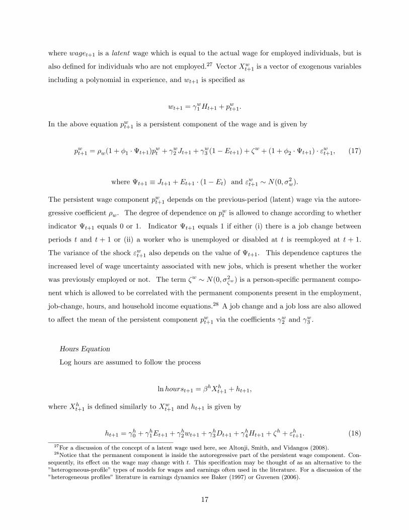
where waget+1 is a latent wage which is equal to the actual wage for employed individuals, but is

also de�ned for individuals who are not employed.27 Vector Xwt+1 is a vector of exogenous variables

including a polynomial in experience, and wt+1 is speci�ed as

wt+1 = w1Ht+1 + p

wt+1:

In the above equation pwt+1 is a persistent component of the wage and is given by

pwt+1 = �w(1 + �1 �t+1)pwt + w2 Jt+1 + w3 (1� Et+1) + �w + (1 + �2 �t+1) � "wt+1; (17)

where t+1 � Jt+1 + Et+1 � (1� Et) and "wt+1 � N(0; �2w).

The persistent wage component pwt+1 depends on the previous-period (latent) wage via the autore-

gressive coe�cient �w. The degree of dependence on pwt is allowed to change according to whether

indicator t+1 equals 0 or 1. Indicator t+1 equals 1 if either (i) there is a job change between

periods t and t + 1 or (ii) a worker who is unemployed or disabled at t is reemployed at t + 1.

The variance of the shock "wt+1 also depends on the value of t+1. This dependence captures the

increased level of wage uncertainty associated with new jobs, which is present whether the worker

was previously employed or not. The term �w � N(0; �2�w) is a person-speci�c permanent compo-

nent which is allowed to be correlated with the permanent components present in the employment,

job-change, hours, and household income equations.28 A job change and a job loss are also allowed

to a�ect the mean of the persistent component pwt+1 via the coe�cients w2 and

w3 .

Hours Equation

Log hours are assumed to follow the process

lnhourst+1 = �hXh

t+1 + ht+1;

where Xht+1 is de�ned similarly to X

wt+1 and ht+1 is given by

ht+1 = h0 +

h1Et+1 +

h2wt+1 +

h3Dt+1 +

h4Ht+1 + �

h + "ht+1: (18)

27For a discussion of the concept of a latent wage used here, see Altonji, Smith, and Vidangos (2008).28Notice that the permanent component is inside the autoregressive part of the persistent wage component. Con-

sequently, its e�ect on the wage may change with t. This speci�cation may be thought of as an alternative to the"heterogeneous-pro�le" types of models for wages and earnings often used in the literature. For a discussion of the"heterogeneous pro�les" literature in earnings dynamics see Baker (1997) or Guvenen (2006).

17

That is, annual hours of work are allowed to depend on employment status at the survey date,

the wage rate, disability, and health. The term �h is person-speci�c and time-invariant, and may

be correlated with the unobserved permanent components in the previous equations. The error

"ht+1 � N(0; �2h) is iid.

Household Income Equation

Log household income is assumed to follow the process

ln incomet+1 = �y1X

yt+1 + yt+1;

where Xyt+1 is de�ned similarly to X

wt+1 and X

ht+1, and yt+1 is given by

yt+1 = y0 +

y1wt+1 +

y2ht+1 +

y3Dt+1 +

y4Ht+1 +

y5Ut+1 + �

y + pyt+1; (19)

pyt+1 = �ypyt + "

yt+1:

Above, Ut+1 is an indicator of unemployment de�ned by Ut+1 = 1� Et+1 �Dt+1. The household

income equation states �rst that household income depends on the wage and work hours of the

head.29 The reason for this dependence is simply that labor earnings of the head are typically

the main component of household income. In addition, (19) allows Dt+1, Ht+1, and Ut+1 to

a�ect household income via components of household income other than the head's earnings, such

as public and private transfers received by the family or labor income of other family members.

Parameters y3, y4, and

y5 are thus likely to capture insurance to shocks to the head's ability to work,

health, or employment status. The household-speci�c permanent component �y is allowed to be

correlated with the permanent components in the employment transitions, job changes, wage rate,

and work hours equations. The factor structure of the various unobserved permanent components

is described below. The component pyt+1 captures the residual unexplained variation in household

income. This residual exhibits important persistence in the data and is thus modeled as an AR(1)

process. The shock "yt+1 � N(0; 1) is iid.

29Recall that when taking the model to the data, wt+1, ht+1, Dt+1, Ht+1, and Ut+1 refer to the head of thehousehold.

18

Permanent Unobserved Heterogeneity

The permanent unobserved components in the above equations are assumed to follow the factor

structure

�EE = �EE� �+ �EE� �

�UE = �UE� �+ �UE� �

�JC = �JC� �+ �JC� � (20)

�w = �w��

�h = �h��+ �h��

�y = �y��;

where � � N(0; 1), � � N(0; 1), and � � N(0; 1) (introduced below) are mutually independent,

individual-speci�c permanent components, and all � coe�cients are factor loadings to be estimated.

Factor � is de�ned as the unobserved heterogeneity component in wages, but it is also allowed to

in uence employment, job changes, and hours. Factor � also a�ects employment, job changes, and

hours, but is assumed to have no in uence on wages. The latter component is intended to capture

factors related to labor supply and to job and employment mobility preferences. Factor � in the

income equation is de�ned as � = ��+p1� �2� and is thus � N(0; 1) and correlated with �, with

correlation coe�cient � (which is also estimated).

4.3.2 Estimates of the Income Model

The employment, job mobility, wage rate, work hours, and household income equations presented

above are estimated jointly by generalized indirect inference.30 Appendix 4 describes implemen-

tation of the estimation method used here.31 In order to estimate the e�ects of disability and

health in equations (13) - (19) I simulate Dt and Ht using the estimates of equations (11) and (12)

presented above. Estimation in this section is thus conditional on the estimated parameters of the

disability and health processes.

30The coe�cients on the variables in vectors Xwt , X

ht , and X

yt , however, are not estimated by indirect inference.

Variation due to variables in the Xt vectors is removed from the data using a �rst-stage regression prior to estimationby indirect inference. Vectors Xw

t and Xht contain a polynomial in experience, education, race, and year indicators.

Vector Xyt contains a number of additional variables (see Appendix 3). The experience polynomial and the sample

average of most of the variables in vector Xyt are added back to the household income equation when calculating

levels of household income to be used in the consumption model.31For a general discussion of the method see Keane and Smith (2003).

19

Estimation results for equations (13) - (19) are presented in Table 2C. I will not discuss the

estimated parameters of all equations here. Instead, I will focus on the main features of the

estimates of the wage and household income equations only. The next section will use simulations

to provide an informal evaluation of the �t of all estimated equations and will thus illustrate some of

the implications of the estimated parameters in the employment, job change, and hours equations.

Panel (d) in Table 2C presents estimates of the wage equation. The most important features

of the estimates are the following. Persistence in the wage rate is high but well below unity (the

autoregressive coe�cient �w is 0:939). The standard deviation �w of the wage shock "wt+1 for

job stayers is fairly large (0:097). When wage shocks involve a new job (whether the job change

involves going through a period of nonemployment or not) the standard deviation of the wage shock

more than triples to 0:298 (�1 = 2:054), and the dependence on the lagged wage falls to 0:794

(�2 = �0:154). New jobs are thus associated with substantial wage risk. Finally, nonemployment

is negatively related to the persistent wage component through the coe�cient b w3 = �0:140.Panel (f) presents the estimated parameters of the household income equation. The most

important features of the estimates are the following. Wages and hours have a strong positive

association with household income (coe�cients y1 and y2 are 0:592 and 0:454, respectively). Con-

ditional on the wage and hours, disability is positively related to household income (coe�cient y3

is 0:186). This positive relationship is likely to re ect transfers from disability insurance but could

also re ect a positive labor supply response of a spouse or other family members to disability of the

head. In either case, the positive coe�cient suggests the presence of substantial insurance against

disability shocks.

Contrary to disability, health limitations do not have a positive association with household

income conditional on the wage and hours (coe�cient y4 is �0:007). There is thus no evidence

of insurance against health limitations captured by H. Unemployment does have have a positive

relationship, but the coe�cient is small ( y5 = 0:027).

The results further indicate that permanent unobserved heterogeneity in household income is

important (�y

� = 0:248) and negatively correlated with unobserved heterogeneity in the employment,

job mobility, wage rate, and hours equations (� = �0:148). One possible explanation is that

households who do permanently better in the labor market may also receive permanently less

transfers from public programs. Another possible explanation is that permanently higher earnings

of the head may permanently reduce the labor supply of a spouse if present. Finally, the serially

correlated error in household income pyt (i.e., the residual household income component) has an

20

autoregressive coe�cient of �y = 0:449 and a large standard deviation of �y = 0:168.

4.4 Medical Expenditures

Out-of-pocket medical expenditures in old age are assumed to be given by32

Mt+1 = exp( M0 + M1 (t+ 1) +

M2 (t+ 1)

2 + M3 (t+ 1)3 + M4 Ht+1 + p

Mt+1) (21)

pMt+1 = �M � pMt + "Mt+1;

where V ar["Mt+1] = �2M . The log of medical expenditures lnMt+1 thus depends on a deterministic

polynomial in age, health status, and a persistent component pMt+1 which follows an AR(1) process.33

The coe�cients in equation (21) are estimated by �tting a least-squares regression of lnMt+1.

Any unobserved permanent component a�ecting medical expenditures is assumed to be captured

by the permanent component in health.34 Parameters �M and �2M are estimated by �tting sample

autocovariances of the least-squares regression residuals to theoretical autocovariances implied by

the �rst-order autoregressive assumption on the error term. Autocovariances are �tted using an

equally-weighted minimum distance estimator.35

Table 2D presents the estimated parameters. The age pro�le is not very pronounced: the

polynomial in t is initially increasing, then decreasing, and then increasing again. Health limitations

have a signi�cant positive relationship with medical expenditures. If one sets the persistent shock

pMt+1 to zero, for instance, expected medical expenditures at t = 50 are $413 for someone in good

health and $640 for someone in poor health. Uncertainty in medical expenditures is large (�M =

0:936) and the shocks are fairly persistent (the autoregressive coe�cient is �M = 0:745).36

32Similar speci�cations are used in Hubbard, Skinner, and Zeldes (1994, 1995) and Scholz, Seshadri, and Khita-trakun (2006), among others.33Notice that the disability indicator Dt does not enter equation (21). The reason is that Dt is a variable related

to employment status and is not a state variable in old age in the lifecycle model.34Equation (21) does not allow for permanent unobserved heterogeneity other than that entering through health.

The reason is that from the point of view of the lifecycle, medical expenditures in old age are assumed to be unknownearly in life and are thus treated as risk.35For evidence in favor of using equal weights rather than an optimal weighting scheme see Altonji and Segal (1996).36Scholz, Seshadri, and Khitatrakun (2006) use a model similar to equation (21) and a measure of medical ex-

penditures similar to the one used here but constructed from the Health and Retirement Study. They estimatethe persistence parameter to be around 0.84 and 0.86, and a standard deviation of the shock which ranges from0:512 for married households with college education to 2:081 for single households with no college. Reported medicalexpenditures of zero are set in their analysis to $1.00 (i.e., 0 in logs). I �nd that setting expenditures of zero to$1 considerably in ates the persistence of shocks. The reason is that very low values of expenditures (such as zeroexpenditures) tend to be more persistent than large values. This turns out to a�ect the estimates of persistencesigni�cantly. Setting zero expenditures to $1 in a log speci�cation also implies that percentage changes at very lowlevels of expenditures have the same e�ect as similar percentage changes at high levels of expenditures. It wouldgenerally be more appropriate to set zero expenditures in a log model to some higher minimum level, say $300.

21

4.5 Evaluation of Fit

This section provides an informal evaluation of the �t of the processes estimated in the previous

section by simulating data from the estimated processes, and then comparing sample statistics of

the simulated data against sample statistics of the PSID data. I simulate data from the estimated

equations for a large number of individuals and then randomly select a subsample of the simulated

data in such a way that its demographic pattern matches that of the PSID sample.

Table 3A presents the sample mean of the disability and health limitations indicators for dif-

ferent levels of potential experience. The column under the "Overall" heading displays statistics

for all levels of potential experience. The next columns report results for the level of t indicated

in the top row. For each reported level of experience, the results combine data for periods t � 1,

t, and t+ 1. For instance, t = 5 uses data for t = 4; 5; and 6. As the �gures show, the simulated

data match the PSID data fairly closely. The overall mean of D is 0:02 in both the PSID and the

simulated data. The probability that D equals 1 increases steadily with experience. For health

limitations, the overall mean is 0:13 in the PSID and 0:14 in the simulations. The probability that

H = 1 also increases steadily with experience. For high levels of experience (t around 60), these

probabilities are 0:50 in the PSID and 0:54 in the simulated data.

Table 3B presents similar statistics for all variables used in the estimation of the joint household

income process.37 I will not attempt to discuss all statistics here. The main points to notice in

Table 3B are the following. (i) The overall �t of the simulated data is good. (ii) The main aspect

that is missed by the simulations is a fairly strong and steady increase in the standard deviation

of log hours with potential experience. This increase translates into a similar rise in the standard

deviation of labor earnings of the head and, to a lesser extent, of household income. This feature

of the PSID data appears to re ect the fact that exceptionally low levels of reported hours become

more common with large values of potential experience. This, in turn, is likely to be the result of

workers retiring gradually and signi�cantly reducing their hours of work prior to full retirement.

Finally, Table 3C presents statistics for the estimated medical expenditures process. Overall,

the �t seems fair given the somewhat erratic pattern observed in the data. The overall mean is

1:576 in the PSID and 1:342 in the simulated data. The overall standard deviation is 3:758 in the

However, in the case of medical expenditures, this distorts the estimates signi�cantly because of the large number ofzeros in the distribution. The approach taken here is to use only positive values of expenditures in the estimation.This will overestimate the probabilities of facing medical expenditures. However, this approach still implies smallerexpenditures (and smaller persistence) than setting $0 observations to any amount that is below about $300.37The table also displays statistics for employment duration, unemployment duration, job duration, and labor

earnings. Even though these variables do not appear in the consumption model, they are used in estimation of thejoint model of employment, job changes, wage, hours, and income. See Appendix 3 and Appendix 4.

22

PSID and 3:519 in the simulations.

5 Solution to the Lifecycle Model

Once parameterized, the lifecycle model is solved by numerical dynamic programming. The model

gives rise to three di�erent forms of Bellman equations, corresponding to (i) the working years,

(ii) the transition between work and retirement, and (iii) the retirement years, respectively. The

Bellman equations are as follows:

Working years

V (t;Dt;Ht; Et; pwt ; p

yt ; zt) = maxfu(ct)

+�E [V (t+ 1; Dt+1;Ht+1; Et+1; pwt+1; p

yt+1; zt+1)

jt;Dt;Ht; Et; pwt ; pyt ; zt]g; (22)

where the expectation, given transition equations (1) - (6), is taken over shocks "Dt+1, "Ht+1, "

EEt+1,

"UEt+1, "DEt+1, "

Jt+1, "

wt+1, "

ht+1, "

yt+1.

Last working year

V (t;Dt;Ht; Et; pwt ; p

yt ; zt) = maxfu(ct)

+��tEt[V (t+ 1;Ht+1; pMt+1; SSt+1; zt+1)

jt;Dt;Ht; Et; pwt ; pyt ; zt]g; (23)

where the expectation, given transition equations (2), (7), and (10) is taken over shocks "Ht+1 and

"Mt+1.

Retirement years

V (t;Ht; pMt ; SSt; zt) = maxfu(ct)

+��tEt[V (t+ 1;Ht+1; pMt+1; SSt+1; zt+1)

jt;Ht; pMt ; SSt; zt]g; (24)

where the expectation, given transition equations (2) and (8) - (10) is taken over "Ht+1 and "Mt+1.

23

In solving the model, cash on hand zt and the persistent wage component pwt are treated as

continuous state variables. Consumption ct is also continuous. State variables pyt and pMt are

approximated by Markov chains, and SSt+1 is also discretized. Since the dynamic programming

problem has a �nite horizon, the Bellman equations are solved by value function iteration. The

largest computational costs of solving the Bellman equations in this model arise from computing

the expectations of the next-period value function. Expectations are computed as follows: For

state variables Dt, Ht, and Et, I use estimated equations (11)-(15), and pseudo-random draws of

"Dt+1, "Ht+1, "

EEt+1, "

UEt+1, "

DEt+1, to simulate the joint behavior of Dt, Ht, and Et. From the simulation,

I compute matrices of transition probabilities for a vector (Dt, Ht, Et) and use these transition

matrices to compute the expectations. For state pyt , I use the transition probabilities associated

with the Markov chain approximation. Finally, I use Gauss-Hermite quadrature to compute

expectations with respect to "Jt+1, "ht+1, and "

wt+1.

Treating cash on hand and the persistent wage component as continuous requires the use of an

interpolation scheme to evaluate next-period's value function at arbitrary values of the continuous

state variables. I use bicubic interpolation. This preserves di�erentiability of the right-hand side of

the Bellman equation and allows solving each optimization problem using Newton-Raphson, which

is convenient because of its fast (quadratic) convergence. All programs are written in Fortran 90

and parallelized using MPI (Message Passing Interface).

5.1 Optimal Consumption Behavior

This section discusses some of the properties of the solution to the lifecycle consumption model

presented above. The data were treated, and the model was parameterized, so that income and

consumption are in thousands of year-2000 dollars. The model corresponds to a household of

mean size and composition, with mean years of education, whose head is white, and who is at the

mean of the distribution of permanent unobserved heterogeneity components. All aggregate risk

is abstracted from in the model.38

Figure 1 presents mean experience pro�les for household nonasset income and consumption,

both simulated from the baseline lifecycle model. The nonasset income pro�le has a humped

shape, with a signi�cant drop at the time of retirement. The drop at retirement is particularly

pronounced because the current parameterization of nonasset retirement income in the model uses

only social security bene�ts of the household head.39 The mean pro�le of (optimal) consumption

38Year e�ects are removed from the wage, hours, earnings, and household income data prior to estimation.39It is straightforward to include social security bene�ts of a spouse and dependents. One could also consider a

second type of household which additionally receives de�ned bene�t pensions. The inclusion of additional components

24

is also hump-shaped, but smoother than income. Mean consumption in the �gure never exceeds

mean income. This is because of the presence of borrowing constraints along with the assumption

in the simulations that households begin their career with zero initial assets.40

Figures 2 - 5 display optimal consumption rules and their dependence on the value of the various

state variables in the model. Figure 2 exhibits optimal consumption as a function of cash on hand

for an employed household in good health in period 1 (�rst year of career) who is at the mean

of the distribution of the persistent wage and household income components pwt and pyt . At low

levels of cash on hand, households are credit-constrained and consume their entire wealth. Above

a certain threshold, households begin to save. This behavior is typical of consumption models with

precautionary motives.41

Figure 3 illustrates the dependence of optimal consumption on the level of the residual compo-

nent of household income pyt in period 1 (�rst year of career) for an employed individual in good

health who is at the mean of the wage distribution. The �gure displays consumption policy func-

tions for values of pyt ranging from 2 standard deviations above to 2 standard deviations below the

mean. The �gure indicates that, conditional on having $20,000 in cash on hand in its �rst year of

career, a household with component pyt two standard deviations above the mean will spend about

$3,000 more on consumption than a household with pyt two standard deviations below the mean.

Figure 4 shows the dependence of consumption on the persistent wage component pwt . The

�gure refers to a household who is employed, in good health, and at the mean of the household

income component pyt in period 1. A higher current wage leads to a higher level of consumption

for a given level of resources. The �gure corresponds to values of pwt ranging from 2.8 standard

deviations above to 2.8 standard deviations below the mean. Conditional on having $30,000 in

total resources in its �rst year of career, a household with component pwt 2.8 standard deviations

above the mean will spend about $12,000 more on consumption than a household with pwt 2.8

standard deviations below the mean. Figure 5 displays the optimal consumption rule over the

entire range of possible realizations that pwt may take in the simulations.42

of retirement income will make the drop less pronounced and will tend to reduce saving for retirement purposes. It willnot a�ect uncertainty, however, which is the main object of interest here. The important aspects of retirement nonassetincome here are that (i) income drops at the time of retirement, and (ii) there is no uncertainty after retirementin social security receipts. One possible extension that would introduce an additional source of uncertainty duringretirement which seems relevant would be to account for uncertainty in rates of return and hence in endogenous assetincome. One important aspect to consider in such an extension is that a high degree of heterogeneity in participationin the stock market implies that uncertainty in rates of return is likely to be highly heterogeneous across households.40All assumptions used in the simulations are discussed in more detail in the next section.41See, for instance, Deaton (1991), Carroll (2001), Gourinchas and Parker (2002), or Cagetti (2003). Optimal

behavior is qualitatively similar whether borrowing constraints are exogenously imposed or arise as "natural" con-straints, using the terminology introduced by Aiyagari (1994).42Recall that both the persistent wage pwt and cash on hand zt are treated as continuous state variables in the

25

The �gures give a sense of the e�ects on optimal consumption of changes in a particular state

variable, holding the rest constant. Changes in most state variables, such as a change in employ-

ment status, however, lead to same-period changes in other state variables. The next section uses

simulations to analyze various implications of the lifecycle model, accounting for all interactions

among the di�erent variables.

6 Simulation Analysis

This section uses simulations to investigate the implications of the consumption and income models

for the importance of the various sources of income risk for household welfare and precautionary

saving. The analysis is based on numerically solving and then simulating the consumption model for

a large number of households under a variety of scenarios. The scenarios di�er in the number and

type of shocks facing the households, who behave optimally under each scenario. In all simulations,

households are assumed to begin their career with zero initial assets. The determination of initial

conditions for the key simulated processes is discussed in more detail in Appendix 3.

6.1 Welfare Gains of Insuring Speci�c Sources of Risk

This subsection evaluates the welfare gains to the household from fully insuring against each speci�c

source of income risk. We will consider two di�erent insurance schemes. In the �rst, which will

be called the unadjusted case, full insurance means the following: For any given shock, an insured

household is compensated (by a lumpsum transfer) upon the realization of the shock in such a way

that the realization of the shock has no e�ect on the realization of income. For instance, insuring

unemployment risk means that in the event of unemployment the household receives a transfer that

exactly o�sets the income lost due to the unemployment shock. Thus, income after the insurance

transfer is exactly the same as it would have been had the worker remained employed. As another

example, fully insuring wage risk means that the insured household's income after the transfer will

be the same, regardless of the actual realization of the wage shock, as it would have been had the

realization of the wage shock been zero.

Insuring risk in this way has two e�ects. First, insurance reduces the variance (uncertainty)

in income associated with a particular source of risk. Second, insurance may also a�ect the mean

of income.43 This bring us to the second insurance scheme, which will be called the adjusted case.

numerical solution of the model.43The reason why insurance a�ects mean income varies somewhat across di�erent shocks. For instance, the occur-

rence of disability, health, and unemployment shocks always a�ects income negatively. Hence, fully insuring againstthese risks raises expected income. Wage, hours, and household income shocks, on the other hand, a�ect expected

26

In this case, mean income in the insured scenario will be adjusted so that it equals mean income

in the uninsured scenario for each year in the lifecycle. That is, the household is required to pay

an actuarially fair premium for insurance, and as a result expected household income is the same

under both the insured and uninsured scenarios. In this sense the insurance considered here is

actuarially fair. Insurance is also full or complete in that it eliminates all uncertainty in income

created by the presence of a particular source of risk. Most of the discussion that follows will focus

on the adjusted case, although for completeness, I will also present results for the unadjusted case

(where mean income in the insured scenario is allowed to be di�erent from mean income in the

uninsured scenario).

Two additional points about the insurance experiment and welfare analysis are worth stressing.

First, the insurance considered here is in addition to already existing insurance mechanisms which

are captured by the household nonasset income process estimated on PSID data.44 Second, in all

cases, households in the model adjust their behavior optimally to the provision of the additional

insurance.

The welfare gains of insurance are calculated in terms of the "equivalent compensating variation"

in consumption. That is, the welfare calculations ask the following question: What percentage of

current lifetime consumption would households be willing to pay in order to be fully insured against

a particular source of risk? The metric used for welfare comparisons is expected lifetime utility at

time zero. This is the expected lifetime utility right before an individual begins their career and

before any uncertainty (other than the household's type) is resolved. This metric is given by:

W = E0[TXt=1

�t�1�tu(c�(t))] =

Z[TXt=1

�t�1�tu(c�(t))]d�; (25)

where t is the state vector, c�(t) is the consumption policy function, which prescribes the

optimal level of consumption at any given point in the state space (i.e., at any possible contingency

that the household may encounter), and � denotes the joint distribution of the random state vector

= (1; :::;T ).45

wage, hours and household income because these variables have log-normal distributions. Hence, although the shocksare symmetric around zero, a change in the variance of the processes also a�ects their mean.44Recall that the household nonasset income data used to estimate the income process includes labor income of all

household members and transfers from outside the household, whether from public or private sources.45Let WU denote welfare under the full-uncertainty scenario and WI denote welfare under the insured scenario.

As explained above, the insured scenario compensates the e�ects of a particular source of risk such that the risk hasno e�ect on net income. The "equivalent compensating variation" is then de�ned as the value of parameter � which

solves the equation W ((1 + �)c�(t)) =WI . Solving for � yields � =�WI+KWU+K

� 11�� � 1; where K = 1

1��PT

t=1 �t�1�t.

This is the measure of welfare gains of insurance (alternatively, welfare costs of risk) used below.

27

6.1.1 Results

Table 4 presents results for the welfare gains of insuring each source of risk for the baseline con-

sumption model. Panel (a) presents adjusted results (the case of actuarially fair insurance), while

panel (b) shows unadjusted results. The entries in columns (1), (2), and (3) of panel (a) indicate

that the welfare gains of fully insuring disability, health, and unemployment risk are extremely

small. According to the table, households are willing to pay no more than 0:04 of 1% of lifetime

consumption in exchange for full insurance against these risks. The welfare value of insurance is

small even if one does not adjust for the e�ect of insurance on mean income. As panel (b) shows,

the value of insuring disability and health risks in the unadjusted case is still no larger than 0:04 of

1% of lifetime consumption. The value of insuring unemployment in the unadjusted case is 0:62

of 1% of lifetime consumption.

Column (5) displays the results for wage shocks. These shocks are innovations in the hourly

wage which are not related to changes in employment status or in employer. As the table shows,

households in the baseline model would be willing to pay up to 1:20% of their lifetime consumption

in order to be insured against such shocks.

Columns (6), (7), and (8) present the gains of insuring shocks associated with job changes,

hours of work, and the residual component of household income. The equivalent compensating

variation in these cases is 0:72%, 0:45%, and 2:19%, respectively.46 I don't discuss the results for

medical expenditures here, as these are preliminary (see discussion in section 2).

6.1.2 Discussion

Overall, the results in Table 4 indicate that the value of insuring most sources of risk in the model

is small. Particularly striking is how minuscule consumers' willingness to pay for insurance against

disability, health, and unemployment risks turns out to be. It is also remarkable how much more

valuable insurance against wage shocks is. These results, however, are consistent with Low, Meghir,

and Pistaferri (2006), who study the welfare e�ects of unemployment and wage shocks, and �nd

that wage risk is important, but that unemployment risk is not.

The shock to the residual component of household income turns out to play a very important

role. This is perhaps not surprising, considering that this shock captures all variation in household

income which is not explained by earnings, disability, health, or unemployment of the head, and

46Notice that job-mobility shocks also operate mostly through an e�ect on the wage rate. The di�erence with wageshocks is that the latter do not involve a change of employer.

28

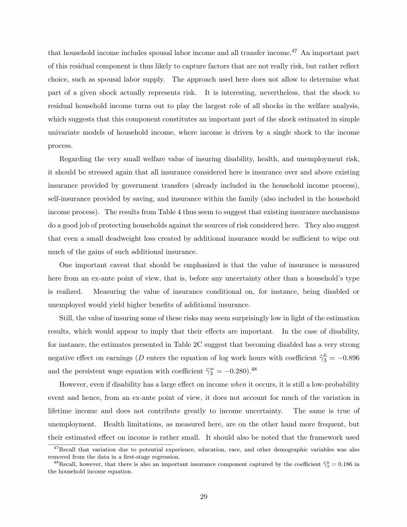
that household income includes spousal labor income and all transfer income.47 An important part

of this residual component is thus likely to capture factors that are not really risk, but rather re ect

choice, such as spousal labor supply. The approach used here does not allow to determine what

part of a given shock actually represents risk. It is interesting, nevertheless, that the shock to

residual household income turns out to play the largest role of all shocks in the welfare analysis,

which suggests that this component constitutes an important part of the shock estimated in simple

univariate models of household income, where income is driven by a single shock to the income

process.

Regarding the very small welfare value of insuring disability, health, and unemployment risk,

it should be stressed again that all insurance considered here is insurance over and above existing

insurance provided by government transfers (already included in the household income process),

self-insurance provided by saving, and insurance within the family (also included in the household

income process). The results from Table 4 thus seem to suggest that existing insurance mechanisms

do a good job of protecting households against the sources of risk considered here. They also suggest

that even a small deadweight loss created by additional insurance would be su�cient to wipe out

much of the gains of such additional insurance.

One important caveat that should be emphasized is that the value of insurance is measured

here from an ex-ante point of view, that is, before any uncertainty other than a household's type

is realized. Measuring the value of insurance conditional on, for instance, being disabled or

unemployed would yield higher bene�ts of additional insurance.

Still, the value of insuring some of these risks may seem surprisingly low in light of the estimation

results, which would appear to imply that their e�ects are important. In the case of disability,

for instance, the estimates presented in Table 2C suggest that becoming disabled has a very strong

negative e�ect on earnings (D enters the equation of log work hours with coe�cient b h3 = �0:896and the persistent wage equation with coe�cient b w3 = �0:280).48

However, even if disability has a large e�ect on income when it occurs, it is still a low-probability

event and hence, from an ex-ante point of view, it does not account for much of the variation in

lifetime income and does not contribute greatly to income uncertainty. The same is true of

unemployment. Health limitations, as measured here, are on the other hand more frequent, but

their estimated e�ect on income is rather small. It should also be noted that the framework used

47Recall that variation due to potential experience, education, race, and other demographic variables was alsoremoved from the data in a �rst-stage regression.48Recall, however, that there is also an important insurance component captured by the coe�cient b y3 = 0:186 in

the household income equation.

29

here only considers the e�ects of disability and health on income and abstracts from direct e�ects

on utility. Such e�ects are likely to be important for welfare.

One additional reason that helps explain the small value of insurance obtained and which should

be mentioned here is that for the broad measure of household income taken from the PSID, income

very rarely falls below $1; 000 (in year-2000 dollars). Consequently, income shocks in the lifecycle

model are discretized in such a way that household income in the model can never fall below

$1; 000. This is important for welfare because under constant relative risk aversion (CRRA) utility

the really painful events occur when consumption drops to extremely low levels. The presence of

an income oor e�ectively provides a consumption oor, ruling out situations where consumption

is near zero. The view taken here is that the oor of $1; 000 per year used in the calculations is

very conservative, given that people have access to a wide array of transfers. Thus, a more precise

way to interpret the results in this paper may be that, if one is willing to assume that constant

relative risk aversion utility is a reasonable representation of preferences and that existing safety

nets provide a minimum level of income and consumption as low as $1; 000 a year, then the value

of insuring risk over and above already existing insurance is small.

It may also be worth mentioning that ignoring some margins of choice in the model, such as

labor supply, has an ambiguous impact on the value of insurance. In the simulated model, treating

labor supply as �xed forces consumption to take on the full e�ects of the shocks, which thus turn

out to be more painful than they would otherwise be. However, keeping labor supplied �xed in

estimation of the income process also a�ects the estimates of risk. A given observed variation in

income may re ect demand shocks that are partially absorbed and o�set by an adjustment in labor

supply, and this adjustment has a welfare cost. Thus, allowing for exible labor supply in the

estimation and in the simulation could make the results change either way.

Finally, Table 7A presents results obtained under alternative assumptions regarding the house-

hold's degree of risk aversion and patience. Panel (a) (second row) displays results for households

with a coe�cient of relative risk aversion of 5:0.49 As should be expected, the higher degree of

risk aversion increases the value of insurance for all sources of risk. However, the increase in the

coe�cient of relative risk aversion to a value as high as 5:0 does not change any of the main results

or conclusions drawn from the analysis above. In particular, the value of insuring disability, health,

and unemployment risk remains minuscule, and the relative importance of the various sources of

49As noted above, the value 5:0 is at the high end of values generally considered empirically plausible. See discussionin note 17. I do not consider values of the coe�cient of risk aversion smaller than 3:0 because they would lead to aneven smaller value of insurance than in the baseline case.

30

risk does not change. Panel (b) displays results for di�erent values of the discount factor. The

numbers in the table suggest that the importance of the residual component of household income

increases as impatience increases, while the wage component appears to become less important.

One possible reason for this is that the wage a�ects social security bene�ts, and thus may a�ect

future periods more than the residual component of household income does. Most importantly,

the results regarding disability, health, and unemployment do not change signi�cantly. Overall,

we conclude that the most important features of the results are robust to alternative, empirically

plausible assumptions about household preferences.

6.2 Precautionary Saving

This section investigates the contribution of the various sources of uncertainty to the accumulation

of precautionary savings. Figure 6 displays the mean level of assets held by simulated households,

by year of potential experience. The upper curve represents mean asset holdings under the full-

uncertainty scenario, while the lower curve displays mean asset holdings under no uncertainty. The

mean pro�le of net income is identical under both scenarios. The di�erence between the two curves

is mean precautionary wealth, that is, the mean level of assets held only because of the presence of

uncertainty. Figure 7 displays this di�erence.50

Figure 8 displays mean precautionary wealth as a fraction of total wealth. The �gure shows

that precautionary savings make up the entirety of savings for the �rst 11-12 years of a worker's

career. Workers start saving for lifecycle reasons (retirement) only after this point. Even 20 years

into a worker's career, precautionary wealth continues to make up 50% or more of total savings.

The exact point at which retirement saving begins to matter will depend on how substantial the

drop in income at retirement is. The current version of the lifecycle model analyzed here does not

account for de�ned bene�t pensions or social security bene�ts received by family members other

than the household head. As a result, income drops signi�cantly at retirement and workers start

saving for retirement relatively early in their career.

Table 5 decomposes precautionary wealth into components attributable to various sources of

risk. Speci�cally, the table calculates the di�erence between mean precautionary wealth under full

uncertainty and mean precautionary wealth under a scenario in which one particular source of risk

is fully insured, and then expresses this di�erence as a percentage of mean precautionary wealth.

Contributions are normalized to sum to 100% of precautionary wealth51. The results in the table

50Like most consumption models, the model used here does not distinguish between liquid and illiquid assets. Inparticular, the model does not separately allow for real estate wealth. Intergenerational transfers are also ignored.51Without the normalization, their sum slightly exceeds 100% because of interactions among the di�erent sources

31

show that the largest contribution by far is made by shocks to the residual component of household

income (43% of precautionary wealth). Wage shocks are also very important, contributing almost

20% of precautionary wealth. Together, these two sources thus account for about 63%. The

individual contribution of all other shocks is below 20%. Among these, job-mobility shocks make

the largest contribution (9:34%) and disability shocks the smallest (2:34%).

Table 7B presents results from a similar decomposition under alternative assumptions about the

coe�cient of relative risk aversion and discount factor. As above, Panel (a) considers households

with a coe�cient of risk aversion of 5.0, while Panel (b) considers households with an increasing

degree of impatience. As the numbers in the table show, the relative importance of the various

sources of risk for the accumulation of precautionary saving does not appear to be sensitive to

alternative assumptions about risk aversion and patience. More generally, the results for precau-

tionary saving seem consistent with the welfare results from the previous section, and the general

discussion presented in that section also applies here.

7 Conclusions and Research Agenda

This paper uses a lifecycle consumption model to quantify the e�ects of a number of sources of

income risk on household welfare and precautionary saving. The model includes income shocks

associated with disability, health, unemployment, job changes, wages, work hours, and a residual

component of household income. I estimate the processes driving the evolution of these variables

using PSID data, accounting for permanent unobserved heterogeneity {which is assumed to be

known at the beginning of a worker's career{ and a rich set of dynamic interactions among the

variables. I then use the consumption model to quantify the welfare value of providing full,

actuarially fair insurance against each source of risk and measure the contribution of each shock to

the accumulation of precautionary savings.

The main �ndings are that: (i) the value of insuring disability, health, and unemployment

shocks is extremely small (well below 1/10 of 1% of lifetime consumption in the baseline model);

(ii) the gains from insuring shocks to the wage and to the residual component of household income

are signi�cantly larger (above 1% and 2% of lifetime consumption, respectively); and (iii) the latter

two shocks account for more than 60% of precautionary wealth.

The insurance evaluated in this paper is insurance over and above existing insurance provided

by government transfers, self-insurance through saving, and insurance within the family, all of

of uncertainty (for instance, the dependence of disability on lagged health limitations).

32

which are already captured in the baseline model. The results thus seem to suggest that existing

insurance mechanisms do a good job of protecting households against the sources of risk considered

here. They also suggest that even a small deadweight loss created by additional insurance would

be su�cient to wipe out much of the gains of such additional insurance.

It should be noted, however, that the value of insurance is measured from an ex-ante point of

view, that is, before any uncertainty other than a household's type is realized. Measuring the value

of insurance conditional on, for instance, being disabled or unemployed should yield higher bene�ts.

Even more importantly, the model analyzed in this paper corresponds to households who are at

the mean of the distribution of the permanent unobserved components. Although the framework

developed here permits analyzing households over the entire distribution of these components, this

is left for future research because of the computational costs of these calculations. It is important

to bear in mind, however, that a clear understanding of the role of heterogeneity is required in

order to draw de�nitive conclusions.

An interesting question that arises from the results presented here regards the value and rel-

ative role of di�erent existing insurance mechanisms. For instance, to what extent are transfers

from disability insurance and unemployment insurance responsible for the small welfare e�ects of

disability and unemployment risk? This particular question may be addressed using this paper's

framework in the following way: (i) remove payments received from disability insurance (alterna-

tively, unemployment insurance) from the income data constructed from the PSID; (ii) estimate

the household income equation presented in section 4 using the modi�ed household income data;

(iii) solve the lifecycle consumption model using the new estimated income process and perform a

welfare analysis. An analysis of the role of these and other sources of insurance is left for future

research.

One potentially important source of risk that is only partially addressed in this paper is the

risk associated with catastrophic medical-expenditure shocks in old age. As discussed earlier,

the treatment in this paper does not allow medical-expenditure shocks to wipe out a household's

accumulated wealth. Some studies, including Palumbo (1999) and De Nardi, French, and Jones

(2006), suggest that the risk of catastrophic medical expenditures may be important for saving

behavior and welfare. A more exible treatment of medical expenditures and their e�ects on

accumulated wealth will be pursued in future work.

33

8 Appendix 1: De�nition of PSID Variables

Potential Experience: Potential labor market experience is de�ned as t = age �max(education;

10)�5 where education is years of education. Labor market experience obtained with less than 10

years of education (which is unusual in the data and typically corresponds to very young individuals)

is not counted as work experience.

Employment Status: The employment indicator E is constructed from the reported employment

status of the head of household at the survey date. The "employment status" PSID variable has

eight possible categories: (1) working now; (2) only temporarily laid o�, sick leave or maternity

leave; (3) looking for work, unemployed; (4) retired; (5) permanently disabled; temporarily disabled;

(6) keeping house; (7) student; (8) other; "workfare"; in prison or jail. Indicator E is set to 1 for

categories (1) and (2); it is set to 0 otherwise.

Disability : The disability indicator D is also based on reported employment status at the survey

date. Indicator D is set to 1 whenever employment status is (5) and it is set to 0 otherwise.

Health Limitations: The health limitations indicator H is constructed from the survey question:

\Do you have any physical or nervous condition that limits the type of work or the amount of work

you can do?" Indictor H is set to 1 when a respondent answers "yes" to the above question, and

it is set to 0 otherwise.

Wage: For hourly workers, the wage variable used is the reported hourly wage at the survey

date. For salaried workers, the variable is constructed from reported weekly, monthly, or yearly

salary, divided by an appropriate standard number of hours. The measure used here further

accounts for the fact that the PSID variable is capped at $9.98 per hour prior to 1978. This

is done by replacing capped values for the years 1975-1977 with predicted values constructed by

Altonji and Williams (2005). Predicted values are based on a regression of the log of the reported

wage on a constant and the log of annual earnings divided by annual hours using the sample of

individuals in 1978 for whom the reported wage exceeds $9.98.

Hours: The hours variable is the reported total annual hours of work (in all jobs).

Household income: Household income is de�ned as the sum of (i) total labor income of the

head; (ii) total labor income of the wife; (iii) total transfer income of the head and wife; (iv)

taxable income of others; and (v) total transfers of others. In most waves, the PSID does not

separately report labor and asset income of other family unit members.

Out-of-Pocket Medical Expenditures: Total out-of-pocket medical expenditures are the sum of

out-of-pocket payments for (i) nursing home and hospital bills; (ii) doctor, outpatient surgery,

34

dental bills; and (iii) prescriptions, in-home medical care, special facilities, and other services. The

payments refer to the two-year period prior to the survey year. Detailed medical expenditures

data are provided by the PSID starting with the 1999 wave.

35

9 Appendix 2: Determination of Social Security Bene�ts

This appendix describes the determination of the level of social security bene�ts. Social security

bene�ts in the model are determined in the last year of work according to the formula:

St+1 = PIA(ALE(Dt;Ht; Et; pwt ; p

yt ))

where PIA stands for principal insurance amount and ALE stands for average lifetime earnings.

Households are assumed to receive a level of bene�ts equal to their PIA. ALE and PIA are

determined as follows.

Average Lifetime Earnings:

In the last working year, the state variables are used to predict average lifetime earnings ac-

cording to a forecasting equation. The coe�cients of the forecasting equation are determined by

simulations of the income (earnings) model using the following procedure:

1. Use the model of disability, health, employment, job changes, wages and hours (which imply

earnings) to simulate a large number of careers.

2. Use the simulated earnings data to compute average lifetime earnings for each simulated

career as calculated by the Social Security Administration. In particular, yearly earnings are

censored from above to the maximum yearly earnings subject to the social security tax. In 1996,

for instance, the maximum taxable yearly amount was $62,700. ALE are then computed as the

average of such censored earnings over the 35 years of highest earnings.

3. Regress ALE against all (simulated) variables that would be known to the agent in the

last year of career in the lifecycle model. These include all state variables in the last working

year (disability, health, employment, persistent wage, persistent household income) as well as all

permanent heterogeneity components (which de�ne the household type). This regression uses a

exible speci�cation which includes a number of higher-order terms and interactions among the

di�erent variables. Several alternatives speci�cations were tried and the regression with the best

�t was selected as the forecasting equation. Estimation results for this forecasting regression are

presented in Table 6. Notice in particular the high R2 in the regression (0:88).

Principal Insurance Amount

Once average lifetime earnings (ALE) have been determined, the principal insurance amount

(PIA) is determined by the rules of the Social Security Administration. I use "bend points" for

the year 1996 (the last year of the sample used in estimation). The 1996 monthly "bend points",

in current dollars, are $437 and $2; 635. The corresponding yearly bend points in thousands of

36

year-2000 dollars are b1 = 5:606 and b2 = 33:801. The PIA, in thousands of year-2000 dollars, is

then calculated as

PIA = 0:90 �minfALE; b1g+ 0:32 �minfmaxfALE � b1; 0g; b2 � b1g+ 0:15 �maxfALE � b2; 0g:

37

10 Appendix 3: Further Details of Model Speci�cation and Esti-

mation - Employment, Job Changes, Wage, Hours, and House-

hold Income

This appendix provides some additional details about the joint model of employment, job changes,

wage rate, work hours, and household income, its estimation, and its relation to the income process

in the lifecycle model.

First Stage Regression and Household Income in Levels

Recall that log household income is given by

ln incomet+1 = �yXy

t+1 + yt+1:

Let Xyt+1 = [Xy

1;t+1; Xy2;t+1; X

y3;t+1] be a partition of X

yt+1 where (i) X

y1;t+1 contains a quadratic

polynomial in age (of the head); (ii) Xy2;t+1 contains years of education of the head and wife as

well as variables describing household size and composition (number of major adults, number of

additional adults, number of children under 6, and number of children between 6 and 18); and

(iii) Xy3;t+1 contains year indicators and race indicators for black and other nonwhite. Vector

�y = [�y1; �y2; �

y3] is estimated in a �rst-stage least-squares regression. Variation in income due to

[Xy2;t+1; X

y3;t+1] is then removed from the data prior to estimation by GII (where the coe�cients of

component yt+1 in equation (19) are estimated). The level of household nonasset income in the

lifecycle model Yt+1 is determined as Yt+1 = exp(ln dincomet+1) = exp(�y1Xy1;t+1+ �

y

2Xy2;t+1+ yt+1),

where Xy2;t+1 is the average of vector X

y2;t+1 in the PSID sample and where yt+1 is the predicted

value of component yt+1.

Initial Conditions

Initial conditions in employment, job changes, the wage, hours, and household income are

explicitly modeled and estimated. For a discussion of related models and further details about

estimation, see Altonji, Smith, and Vidangos (2008).

Employment: Initial employment status is assumed to be determined by E1 = I[b0 + �EE� � +

�EE� � + "EE1 > 0] where b0 � b�0 � �E1, �E1 �q(�EE

� )2 + (�EE

� )2 + 1, �EE� � and �EE� are de�ned as

before, "EE1 � N(0; 1), and b�0 is the coe�cient estimate from a Probit of Et on a constant estimated

on PSID data for t � 3. I use the �rst three years here rather than just the �rst year because

there are relatively few observations when t = 1.

Wages: The initial condition of the persistent wage component is modeled as pw1 = �w�w+uw1;

38

where �w is a free parameter estimated with GII and uw1 � N(0; �2w1); where �2w1 is set such that

V ar(�w�w + uw1) equals the variance of the residual of regression for low levels of t .

Household Income: The initial condition of the residual component of household income is

determined as py1 = �y�y+uy1; where �y is a free parameter estimated with GII and uy1 � N(0; �2y1);

where �2y1 is set such that V ar(�y�y + uy1) equals the variance of the residual of regression for low

levels of t.

Measurement Error

Estimation accounts for measurement error in wages, hours, earnings, and household income.

The treatment of measurement error here follows the treatment in Altonji, Smith, and Vidangos

(2008). For household income, measurement error is set to account for 25% of the variance of the

�rst di�erence in observed household income, after accounting for the e�ect of measurement error in

earnings. Since earnings are a component of household income, one additionally needs to account

for the e�ect of measurement error in earnings on observed household income. Altonji, Smith, and

Vidangos (2008) shows that there is a residual component in earnings which is not accounted for

by wages and hours. This component is assumed here to consist entirely of measurement error.

The system estimated by generalized indirect inference includes an auxiliary equation of earnings

in order to identify this component. Estimates of the household income process account for the

e�ect of this measurement error component.

39

11 Appendix 4: Estimation Mechanics - GII

The equations that determine the evolution of employment, job changes, wage, hours, and household

income are estimated by generalized indirect inference (GII). The implementation of GII used here

is akin to that used in Altonji, Smith, and Vidangos (2008), which provides a detailed discussion.

This appendix gives some further details of the implementation used in this paper. The auxiliary

model consists of a system of seemingly unrelated regressions (SUR) with 8 equations and 27

covariates that are common to all 8 equations. The model is implemented under the assumption

that the errors follow a multivariate normal distribution with unrestricted covariance matrix. The

auxiliary model e�ectively used52 may be written as

yit = Zit�+ uit; uit � N(0;�); uit iid over i and t; (26)

where

yit = [EitEi;t�1; EitUi;t�1; JitEitEi;t�1; (27)

wit; hit; eit; ln(1 + wit2); yit]

0;

52In practice, the auxiliary model actually used in estimation included a few additional covariates. Due to anerror in one of the programs, however, the sorting of the data in the additional covariates was di�erent from thesorting of the data in the rest of the variables, rendering the additional covariates uncorrelated with the rest ofthe variables in the SUR system. Consequently, the auxiliary model e�ectively used is the model described in thisappendix. Excluding the additional covariates altogether from estimation yields estimates that are very close to theones reported in this paper. The additional covariates that were initially intended to be included are Ei, J i, EDi,UDi, JDi, wi;t�1�wi, hi;t�1� hi, ei;t�1� ei, and yi;t�1� yi, where a bar over a variable indicates a person-speci�ctime average.

40

and

Zit = [cons; (t� 1); (t� 1)2; EDi;t�1; UDi;t�1; JDi;t�1; (28)

Ei;t�1Ei;t�2; Ei;t�2Ei;t�3;

Ei;t�1Ui;t�2; Ei;t�2Ui;t�3;

Ji;t�1 � Ei;t�1 � Ei;t�2; Ji;t�2 � Ei;t�2 � Ei;t�3;

wi;t�1; wi;t�2; hi;t�1; hi;t�2; ei;t�1; ei;t�2; yi;t�1; yi;t�2;

wi;t�1(t� 1); wi;t�1(t� 1)2; wi;t�1Jit

Dit; Di;t�1;Hit;Hi;t�1]0:

Above, Uit is an indicator of unemployment de�ned as Uit = 1�Eit �Dit. All other variables

are de�ned as before.

41

References

[1] Abowd, J.M. and Card, D.E. (1987). \Intertemporal Labor Supply and Long-Term Employ-ment Contracts", American Economic Review, 77(1), 50-68.

[2] Abowd, J.M. and Card, D.E. (1989). \On the Covariance Structure of Hours and EarningsChanges", Econometrica, 57(2), 411-445.

[3] Aiyagari, S.R. (1994). \Uninsured Idiosyncratic Risk and Aggregate Saving", QuarterlyJournal of Economics 109(3), 659-684.

[4] Altonji, J.G., Martins, A.P., and Siow, A. (2002). \Dynamic Factor Models of Wages, Hours,and Earnings", Research in Economics 56(1), 3-59.

[5] Altonji, J.G. and Segal, L.M. (1996). \Small Sample Bias in GMM Estimation of CovarianceStructures", Journal of Business and Economic Statistics, 14(3), 353-366.

[6] Altonji, J.G., Smith, A.A., Jr., and Vidangos, I. (2008). \Modeling Earnings Dynamics",unpublished manuscript, Yale University and Federal Reserve Board.

[7] Altonji, J.G. and Williams, N. (2005). \Do Wages Rise With Job Seniority? A Reassessment",Industrial and Labor Relations Review, 58(3), 370-397.

[8] Attanasio, O.P., Banks, J., Meghir, C., and Weber, G. (1999). \Humps and Bumps in LifetimeConsumption", Journal of Business and Economic Statistics, 17(1), 22-35.

[9] Baker, M. (1997). \Growth-rate heterogeneity and the covariance structure of life cycleearnings", Journal of Labour Economics, 15(2), 338-375.

[10] Baker, M. and Solon, G. (2003). \Earnings Dynamics and Inequality among Canadian Men,1976-1992: Evidence from Longitudinal Income Tax Records", Journal of Labor Economics,21(2), 289-321.

[11] Blundell, R. and Pistaferri, L. (2003). \Income Volatility and Household Consumption: TheImpact of Food Assistance Programs", Journal of Human Resources, 38:S, 1032-1050.

[12] Blundell, R., Pistaferri, L., and Preston, I. (2008). \Consumption Inequality and PartialInsurance", American Economic Review, forthcoming.

[13] Blundell, R. and Preston, I. (1998). \Consumption Inequality and Income Uncertainty",Quarterly Journal of Economics, 113(2), 603-640.

[14] Browning, M. and Crossley, T.F. (2001). \Unemployment Insurance Bene�t Levels andConsumption Changes," Journal of Public Economics, 80(1), 1-23.

[15] Burkhauser, R.V., Daly, M.C., Houtenville, A.J., and Nargis, N. (2002). \Self-Reported WorkLimitation Data: What They Can and Cannot Tell Us", Demography, 39(3), 541-555.

[16] Cagetti, M. (2003). \Wealth Accumulation Over the Life Cycle and Precautionary Savings",Journal of Business and Economic Statistics, 21(3), 339-353.

[17] Casta~neda, A., D��az-Gim�enez, J., and R��os-Rull V. (2003). \Accounting for the U.S. Earningsand Wealth Inequality", Journal of Political Economy, 111(4), 818-857.

[18] Carroll, C. (2001). \A Theory of the Consumption Function, with and without LiquidityConstraints", Journal of Economic Perspectives, 15(3), 23-45.

[19] Carroll, C. (1997). \Bu�er-Stock Saving and the Life Cycle/Permanent Income Hypothesis",Quarterly Journal of Economics, 112(1), 1-55.

42

[20] Carroll, C. (1992). \The Bu�er-Stock Theory of Saving: Some Macroeconomic Evidence",Brookings Papers on Economic Activity, 1992(2), 61-156.

[21] Carroll, C. and Samwick, A. (1998). \How Important is Precautionary Saving?", Review ofEconomics and Statistics, 1992(2), 61-156.

[22] Center for Disease Control and Prevention. 2002 Life Tables. U.S. Department of Health andHuman Services. Available at (http://www.cdc.gov/nchs/data/nvsr/nvsr53/nvsr53 06.pdf).

[23] Chetty, R. (2006). \A New Method of Estimating Risk Aversion", American EconomicReview, 96(5), 1821-1834.

[24] Cullen, J.B. and Gruber, J. (2000). \Does Unemployment Insurance Crowd Out SpousalLabor Supply?, Journal of Labor Economics 18(3), 546-72.

[25] Cunha, F., Heckman, J.J., and Navarro, S. (2005). \Separating Uncertainty from Hetero-geneity in Life Cycle Earnings, The 2004 Hicks Lecture", Oxford Economic Papers 57(2),191-261.

[26] Cunha, F. and Heckman, J.J. (2006). \Identifying and Estimating the Distributions of ExPost and Ex Ante Returns to Schooling: A Survey of Recent Developments", unpublishedmanuscript, University of Chicago.

[27] Daly, M.C. and Burkhauser, R.V. (2003). \The Supplemental Security Income Program"in Means-Tested Programs in the United States, edited by R. Mo�tt. National Bureau ofEconomic Research and University of Chicago Press: Chicago, IL.

[28] Daly, M.C. and Houtenville, A. (2003). \Employment Declines Among People with Disabili-ties" in The Decline in Employment of People with Disabilities: A Policy Puzzle, edited by R.V. Burkhauser and D. Stapleton. Upjohn Press, March 2003.

[29] Deaton, A. (1991). \Saving and Liquidity Constraints", Econometrica, 59(5), 1221-1248.

[30] De Nardi, M., French, E., and Jones, J. (2006). \Di�erential Mortality, Uncertain MedicalExpenses, and the Saving of Elderly Singles", Federal Reserve Bank of Chicago WP 2005-13.

[31] Dynan, K.E., Skinner, J., and Zeldes, S.P. (2004). \Do the Rich Save More?", Journal ofPolitical Economy, 112(2), 397-444.

[32] Dynarski, S. and Gruber, J. (1997). \Can Families Smooth Variable Earnings?", BrookingsPapers on Economic Activity, 1, 229-303.

[33] Engen, E.M., Gale, W.G., and Uccello, C.E. (1999). \The Adequacy of Household Saving",Brookings Papers on Economic Activity, 1999:2, 65-165.

[34] Engen, E.M., and Gale, W.G. (1993). \IRAs and Saving in a Stochastic Life-Cycle Model",mimeo, Brookings Institution.

[35] Engen, E.M., Gale, W.G., and Scholz, J.K. (1994). \Do Saving Incentives Work?", BrookingsPapers on Economic Activity, 1994:1, 85-151.

[36] Geweke, J. and Keane, M. (2000). \An empirical analysis of earnings dynamics among menin the PSID: 1968-1989", Journal of Econometrics, 96, 293-356.

[37] Gourieroux, C., Monfort, A., and Renault, E. (1993). \Indirect Inference", Journal of AppliedEconometrics, 8, S85-S118.

[38] Gourinchas, P.O., and Parker, J. (2002). \Consumption over the Life Cycle", Econometrica,70(1) 47-89.

43

[39] Gouveia, M. and Strauss, R. (1994). \E�ective Federal Individual Income Tax Functions: AnExploratory Empirical Analysis", National Tax Journal 47(2), 317-339.

[40] Gouveia, M. and Strauss, R. (2000). \E�ective Tax Functions for the U.S. Individual IncomeTax: 1966{89", Proceedings of the 92nd Annual Conference on Taxation, Atlanta, October24{26. Washington, DC: National Tax Association.

[41] Gruber, J. (1997). \The Consumption Smoothing Bene�ts of Unemployment Insurance",American Economic Review, 87(1) 192-205.

[42] Gruber, J. (1998). \Unemployment Insurance, Consumption Smoothing, and Private Insur-ance: Evidence from the PSID and CEX", Research in Employment Policy, 1, 3-32.

[43] Gruber, J. and Yelowitz, A. (1999). \Public Health Insurance and Private Savings", Journalof Political Economy, 107(6), 1249{74.

[44] Guvenen, F. (2006). \Learning Your Earning: Are Labor Income Shocks Really Very Persis-tent?", American Economic Review, 97(3), 687-712.

[45] Haider, S.J. (2001). \Earnings Instability and Earnings Inequality of Males in the UnitedStates: 1967-1991", Journal of Labor Economics, 19(4), 799-836.

[46] Hall, R.E. and Mishkin, F. (1982). \The Sensitivity of Consumption to Transitory Income:Estimates from Panel Data on Households", Econometrica, 50(2), 461-481.

[47] Hause, J.C. (1980). \The �ne structure of earnings and the on-the-job training hypothesis",Econometrica, 48(4), 1013-1029.

[48] Heaton, J. and Lucas, D.J. (1996). \Evaluating the e�ects of incomplete markets on risksharing and asset pricing", Journal of Political Economy, 104(3), 443-487.

[49] Heckman, J. J. (1981). \The Incidental Parameters Problem and the Problem of InitialConditions in Estimating a Discrete Time - Discrete Data Stochastic Process", in StructuralAnalysis of Discrete Data with Econometric Applications, edited by C.F. Manski and D.McFadden, pp. 179-95. Cambridge: MIT Press.

[50] Hubbard, G., Skinner, J., and Zeldes, S. (1994). \The importance of precautionary motives inexplaining individual and aggregate saving", Carnegie-Rochester Conference Series on PublicPolicy, 40, 59-125.

[51] Hubbard, G., Skinner, J., and Zeldes, S. (1995). \Precautionary Saving and Social Insurance",Journal of Political Economy, 103(2), 360-399.

[52] Huggett, M. (1996). \Wealth Distribution in Life-Cycle Economies", Journal of MonetaryEconomics, 38(3), 469-494.

[53] Hurst, E. and Sta�ord, F. (2004), \Home is Where the Equity Is: Liquidity Constraints,Re�nancing and Consumption," Journal of Money, Credit and Banking, 36(6), 985-1014.

[54] Jacobson, L., LaLonde, R., and Sullivan, D. (1993). \Earnings Losses of Displaced Workers",American Economic Review, 83(4), 685-709.

[55] Keane, M. and Smith Jr., A.A. (2003). \Generalized Indirect Inference for Discrete ChoiceModels", unpublished manuscript, Yale University.

[56] Kniesner, T.J. and Ziliak, J.P. (2002). \Tax Reform and Automatic Stabilization", AmericanEconomic Review, 92(3), 590-612.

[57] Krusell, P. and Smith Jr., A.A. (1997). \Income andWealth Heterogeneity, Portfolio Selection,and Equilibrium Asset Returns", Macroeconomic Dynamics, 1, 387-422.

44

[58] Krusell, P. and Smith Jr., A.A. (1998). \Income and Wealth Heterogeneity in the Macroe-conomy", Journal of Political Economy, 106(5), 867-896.

[59] Lillard, L. and Weiss, Y. (1979). \Components of variation in panel earnings data: Americanscientists 1960-1970", Econometrica, 47(2), 437-454.

[60] Lillard, L. and Willis, R. (1978). \Dynamic aspects of earning mobility", Econometrica,46(5), 985-1012.

[61] Low, H., Meghir, C., and Pistaferri, L. (2006). \Wage Risk and Employment Risk over theLife Cycle", unpublished manuscript, Cambridge University, University College London, andStanford University.

[62] MaCurdy, T.E. (1982). \The use of time series processes to model the error structure ofearnings in a longitudinal data analysis", Journal of Econometrics, 18, 83-114.

[63] Meghir, C. and Pistaferri, L. (2004). \Income variance dynamics and heterogeneity", Econo-metrica, 72(1), 1-32.

[64] Mo�tt, R. (2002). \Documentation for Mo�tt Welfare Bene�ts File", manuscript (February22), Johns Hopkins University, http://www.econ.jhu.edu/People/Mo�tt/DataSets.html.

[65] Palumbo, M.G. (1999). \Uncertain Medical Expenses and Precautionary Saving Near theEnd of the Life Cycle", Review of Economic Studies, 66 (April), 395{421.

[66] Scholz, J.K., Seshadri, A., and Khitatrakun, S. (2006). \Are Americans Saving "Optimally"for Retirement?", Journal of Political Economy, 114(4), 607-643.

[67] Smith, A.A., Jr. (1990). \Three Essays on the Solution and Estimation of Dynamic Macroe-conomic Models", Ph.D. thesis (Duke University).

[68] Smith, A.A., Jr. (1993). \Estimating Nonlinear Time-Series Models using Simulated VectorAutoregressions", Journal of Applied Econometrics, 8, S63-S84.

[69] Stephens, M., Jr. (2002). \Worker Displacement and the Added Worker E�ect", Journal ofLabor Economics, 20(3), 504-37.

[70] Storesletten, K., Telmer, C., and Yaron, A. (2004a). \Consumption and Risk Sharing Overthe Life Cycle", Journal of Monetary Economics, 51(3), 609-633.

[71] Storesletten, K., Telmer, C., and Yaron, A. (2004b). \Cyclical Dynamics in IdiosyncraticLabor Market Risk", Journal of Political Economy, 112(3), 695-717.

[72] Storesletten, K., Telmer, C., and Yaron, A. (2007). \Asset Pricing with Idiosyncratic Riskand Overlapping Generations", Review of Economic Dynamics 10(4), 519-548.

[73] Sullivan, J.X. (2008). \Borrowing During Unemployment: Unsecured Debt as a Safety Net",Journal of Human Resources, forthcoming.

[74] Topel, R. (1991). \Speci�c Capital, Mobility, and Wages: Wages Rise with Job Seniority",Journal of Political Economy, 99(1), 145-176.

[75] Vidangos, I. (2008). \Fluctuations in Individual Labor Income: A Panel VAR Analysis",unpublished manuscript, Federal Reserve Board.

[76] Wooldridge, J.M. (2005), \Simple Solutions to the Initial Conditions Problem for Dynamic,Nonlinear Panel Data Models with Unobserved Heterogeneity", Journal of Applied Economet-rics, 20, 39-54.

45

Table 1ADescriptive Statistics - Disability and Health Samples

All t 1 ≤ t ≤ 10 11 ≤ t ≤ 20 21 ≤ t ≤ 30 31 ≤ t ≤ 40 41 ≤ t ≤ 50 51 ≤ t ≤ 60 61 ≤ t ≤ 65DisabilityObs. 79,545 16,966 29,696 17,872 10,451 4,560Mean 0.022 0.002 0.009 0.025 0.048 0.110

HealthObs. 87,979 16,940 29,686 17,963 10,990 8,206 3,725 469Mean 0.136 0.052 0.081 0.125 0.187 0.313 0.417 0.497

The table displays the number of observations and mean of the disability and health limitations indicator, by cells of potential experience. All cells contain ten years except for the last one, which contains only 5. The statistics displayed correspond to the samples used in estimation of the disability and health models, respectively. The disability sample excludes retired individuals, and all individuals above 64 years of age. After this restriction, the maximum level of potential experience in the sample is 49. All variables are constructed from the PSID.

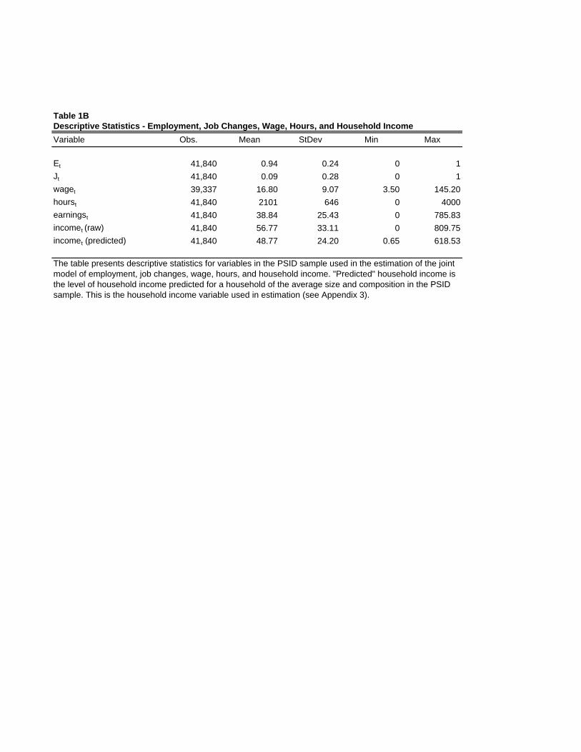
Table 1BDescriptive Statistics - Employment, Job Changes, Wage, Hours, and Household IncomeVariable Obs. Mean StDev Min Max

Et 41,840 0.94 0.24 0 1Jt 41,840 0.09 0.28 0 1waget 39,337 16.80 9.07 3.50 145.20hourst 41,840 2101 646 0 4000earningst 41,840 38.84 25.43 0 785.83incomet (raw) 41,840 56.77 33.11 0 809.75incomet (predicted) 41,840 48.77 24.20 0.65 618.53

The table presents descriptive statistics for variables in the PSID sample used in the estimation of the joint model of employment, job changes, wage, hours, and household income. "Predicted" household income is the level of household income predicted for a household of the average size and composition in the PSID sample. This is the household income variable used in estimation (see Appendix 3).

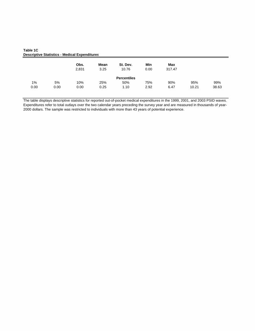
Table 1CDescriptive Statistics - Medical Expenditures

Obs. Mean St. Dev. Min Max2,831 3.25 10.76 0.00 317.47

1% 5% 10% 25% 50% 75% 90% 95% 99%0.00 0.00 0.00 0.25 1.10 2.92 6.47 10.21 38.63

Percentiles

The table displays descriptive statistics for reported out-of-pocket medical expenditures in the 1999, 2001, and 2003 PSID waves. Expenditures refer to total outlays over the two calendar years preceding the survey year and are measured in thousands of year-2000 dollars. The sample was restricted to individuals with more than 43 years of potential experience.

Table 2APoint Estimates and Standard Errors - Disability Indicator (Dt+1)

Variable cons t+1 (t+1)2/100 (t+1)3/1000 Dt Ht ζD

Parameter γD0 γD

1 γD2 γD

3 γD4 γD

5 σζD

Estimate -4.6743 0.0808 -0.1794 0.0251 1.6107 1.1744 0.9343SE (0.2377) (0.0283) (0.1129) (0.0137) (0.0694) (0.0459) (0.0545)

Obs. 87,626

Table 2BPoint Estimates and Standard Errors - Health Limitations Indicator (H t+1)

Variable cons t+1 (t+1)2/100 (t+1)3/1000 Ht ζH

Parameter γH0 γH

1 γH2 γH

3 γH4 σζH

Estimate -2.5656 0.0103 0.0793 -0.0061 1.1191 0.9613SE (0.0597) (0.0070) (0.0248) (0.0026) (0.0203) (0.0198)

Obs. 85,295

The table displays parameter estimates and standard errors of the disability indicator equation. All parameters were estimated by maximum likelihood. The person-specific permanent unobserved component was integrated out of the conditional likelihood function by numerical quadrature. The sample excludes retired individuals, and individuals above 64 years of age.

The table displays parameter estimates and standard errors for the health limitations indicator equation. All parameters were estimated by maximum likelihood. The person-specific permanent unobserved component was integrated out of the conditional likelihood function by numerical quadrature. The sample was restricted to observations where the disability indicator is zero.

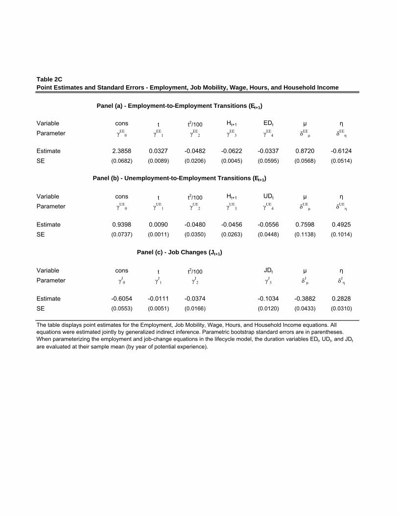
Table 2CPoint Estimates and Standard Errors - Employment, Job Mobility, Wage, Hours, and Household Income

Variable cons t t2/100 Ht+1 EDt μ ηParameter γEE

0 γEE1 γEE

2 γEE3 γEE

4 δEEμ δEE

η

Estimate 2.3858 0.0327 -0.0482 -0.0622 -0.0337 0.8720 -0.6124SE (0.0682) (0.0089) (0.0206) (0.0045) (0.0595) (0.0568) (0.0514)

Variable cons t t2/100 Ht+1 UDt μ ηParameter γUE

0 γUE1 γUE

2 γUE3 γUE

4 δUEμ δUE

η

Estimate 0.9398 0.0090 -0.0480 -0.0456 -0.0556 0.7598 0.4925SE (0.0737) (0.0011) (0.0350) (0.0263) (0.0448) (0.1138) (0.1014)

Variable cons t t2/100 JDt μ ηParameter γJ

0 γJ1 γJ

2 γJ3 δJ

μ δJη

Estimate -0.6054 -0.0111 -0.0374 -0.1034 -0.3882 0.2828SE (0.0553) (0.0051) (0.0166) (0.0120) (0.0433) (0.0310)

Panel (a) - Employment-to-Employment Transitions (Et+1)

Panel (b) - Unemployment-to-Employment Transitions (Et+1)

Panel (c) - Job Changes (Jt+1)

The table displays point estimates for the Employment, Job Mobility, Wage, Hours, and Household Income equations. All equations were estimated jointly by generalized indirect inference. Parametric bootstrap standard errors are in parentheses. When parameterizing the employment and job-change equations in the lifecycle model, the duration variables EDt, UDt, and JDt

are evaluated at their sample mean (by year of potential experience).

Table 2C (continued)Point Estimates and Standard Errors - Employment, Job Mobility, Wage, Hours, and Household Income

Variable Ht+1 pwt Ψt+1 Jt+1 1-Et+1 μ εw Ψt+1

Parameter γw1 ρw Φ1 γw

2 γw3 δw

μ σw Φ2

Estimate -0.0015 0.9389 -0.1538 0.0197 -0.1400 0.0160 0.0975 2.0535SE (0.0421) (0.0029) (0.0093) (0.0045) (0.0089) (0.0019) (0.0020) (0.2766)

Variable cons Et+1 wt+1 Dt+1 Ht+1 μ η εh

Parameter γh0 γh

1 γh2 γh

3 γh4 δh

μ δhη σh

Estimate -0.5258 0.5921 -0.1948 -0.8957 -0.1085 0.2436 0.1284 0.2269SE (0.0089) (0.0080) (0.0160) (0.0192) (0.0065) (0.0093) (0.0114) (0.0014)

Variable cons wt+1 ht+1 Dt+1 Ht+1 Ut+1 λ pyt εy

Parameter γy0 γy

1 γy2 γy

3 γy4 γy

5 δyλ ρy σy κ

Estimate 0.1447 0.5919 0.4535 0.1862 -0.0068 0.0269 0.2478 0.4486 0.1677 -0.1478SE (0.0046) (0.0096) (0.0113) (0.0327) (0.0024) (0.0085) (0.0877) (0.0965) (0.0088) (0.0134)

Panel (e) - Work Hours (ht+1)

Panel (f) - Household Income (yt+1)

The table displays point estimates for the Employment, Job Mobility, Wage, Hours, and Household Income equations. All equations were estimated jointly by generalized indirect inference. Parametric bootstrap standard errors are in parentheses.

Panel (d) - Wage (wt+1)

Table 2DPoint Estimates and Standard Errors - Medical Expenditures (lnM t+1)

Variable cons t+1 (t+1)2 (t+1)3 Ht+1 Family Size year 2001 year 2003Parameter γM

0 γM1 γM

2 γM3 γM

4 γM5 γM

6 γM7 ρM

(1) σM(1)

Estimate -19.9013 1.1011 -0.0209 0.0001 0.4394 -0.1266 0.1391 0.2520 0.7455 0.9356SE (7.5830) (0.3903) (0.0066) (0.0000) (0.0612) (0.0367) (0.0712) (0.0715)

Obs. 2,426Adj R-squared 0.09

The table displays point estimates and standard errors for the medical expenditures equation. The parameters were estimated by least-squares, unless indicated otherwise. Parameters indicated by (1) were estimated by equally-weighted minimum distance matching the 0th, 2nd, and 4th order autocovariances of the residuals of the least-squares equation to those impied by an AR(1) process (the data on medical expenditures are available in two-year intervals only). The sample was restricted to individuals who were retired or had more than 43 years of potential experience. The least-squares regression includes year indicators and controls for family size.

Table 3AEvaluation of Fit: Disability and Health Descriptive Statistics - PSID Sample and Simulated Data

Sample Statistic Model Overall t=5 t=10 t=20 t=30 t=40 t=50 t=60

PSID 0.02 0.001 0.004 0.016 0.030 0.075Simulated 0.02 0.002 0.004 0.014 0.034 0.090PSID 0.13 0.05 0.06 0.11 0.14 0.24 0.37 0.50Simulated 0.14 0.05 0.06 0.10 0.17 0.27 0.40 0.54

Mean Disability

Mean Health Limitations

The table presents descriptive statistics of the PSID sample, and of data simulated from the estimated model. The descriptive statistics of simulated data are based on a simulated sample which is 10 times as large as the PSID sample, but has the same demographic structure (by potential experience) as the PSID sample. All statistics are computed using 3-year windows around the indicated value of t. For instance, t=10 corresponds to sample moments computed over all observations where t=9,10,11. The only exception is t=60, which uses only two years: t=59,60.

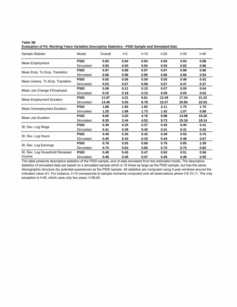
Table 3BEvaluation of Fit: Working-Years Variables Descriptive Statistics - PSID Sample and Simulated Data

Sample Statistic Model Overall t=5 t=10 t=20 t=30 t=40

PSID 0.93 0.94 0.94 0.94 0.94 0.88Simulated 0.93 0.93 0.94 0.93 0.92 0.86PSID 0.97 0.98 0.97 0.97 0.98 0.96Simulated 0.96 0.96 0.96 0.96 0.96 0.93PSID 0.55 0.56 0.59 0.55 0.46 0.42Simulated 0.53 0.57 0.58 0.57 0.47 0.37PSID 0.08 0.21 0.15 0.07 0.05 0.04Simulated 0.10 0.18 0.15 0.09 0.05 0.02PSID 11.87 4.21 6.61 12.49 17.34 21.22Simulated 14.49 5.05 8.78 15.57 20.85 22.55PSID 1.88 1.65 1.82 2.11 1.75 1.70Simulated 1.35 1.68 1.73 1.42 1.07 0.68PSID 9.60 3.00 4.78 9.88 14.98 19.26Simulated 9.35 2.44 4.53 9.73 15.18 18.14PSID 0.39 0.35 0.37 0.40 0.40 0.41Simulated 0.41 0.39 0.40 0.41 0.41 0.42PSID 0.49 0.35 0.42 0.49 0.55 0.75Simulated 0.45 0.43 0.43 0.44 0.48 0.57PSID 0.78 0.55 0.68 0.79 0.85 1.09Simulated 0.70 0.63 0.66 0.70 0.75 0.82PSID 0.49 0.45 0.47 0.50 0.51 0.56Simulated 0.48 0.45 0.47 0.49 0.49 0.50

Mean Employment Duration

Mean Unemployment Duration

Mean Job Duration

Mean Employment

Mean Emp. To Emp. Transition

Mean Unemp. To Emp. Transition

Mean Job Change if Employed

St. Dev. Log Wage

St. Dev. Log Hours

St. Dev. Log Household Nonasset IncomeThe table presents descriptive statistics of the PSID sample, and of data simulated from the estimated model. The descriptive statistics of simulated data are based on a simulated sample which is 10 times as large as the PSID sample, but has the same demographic structure (by potential experience) as the PSID sample. All statistics are computed using 3-year windows around the indicated value of t. For instance, t=10 corresponds to sample moments computed over all observations where t=9,10,11. The only exception is t=40, which uses only two years: t=39,40.

St. Dev. Log Earnings

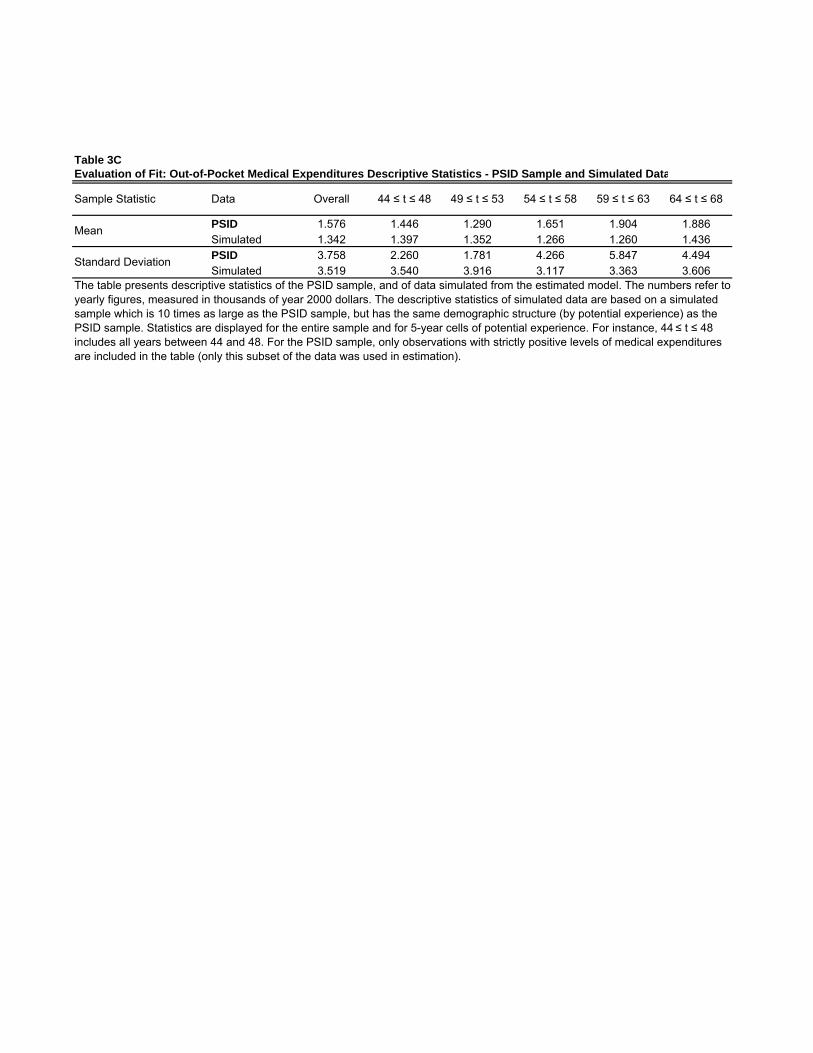
Table 3CEvaluation of Fit: Out-of-Pocket Medical Expenditures Descriptive Statistics - PSID Sample and Simulated Data

Sample Statistic Data Overall 44 ≤ t ≤ 48 49 ≤ t ≤ 53 54 ≤ t ≤ 58 59 ≤ t ≤ 63 64 ≤ t ≤ 68

PSID 1.576 1.446 1.290 1.651 1.904 1.886Simulated 1.342 1.397 1.352 1.266 1.260 1.436PSID 3.758 2.260 1.781 4.266 5.847 4.494Simulated 3.519 3.540 3.916 3.117 3.363 3.606

Mean

Standard Deviation

The table presents descriptive statistics of the PSID sample, and of data simulated from the estimated model. The numbers refer to yearly figures, measured in thousands of year 2000 dollars. The descriptive statistics of simulated data are based on a simulated sample which is 10 times as large as the PSID sample, but has the same demographic structure (by potential experience) as the PSID sample. Statistics are displayed for the entire sample and for 5-year cells of potential experience. For instance, 44 ≤ t ≤ 48 includes all years between 44 and 48. For the PSID sample, only observations with strictly positive levels of medical expenditures are included in the table (only this subset of the data was used in estimation).

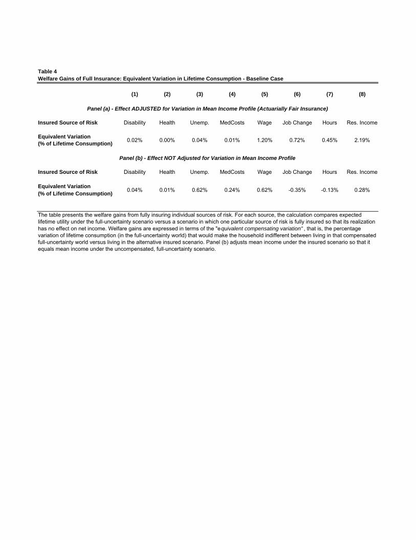
Table 4Welfare Gains of Full Insurance: Equivalent Variation in Lifetime Consumption - Baseline Case

(1) (2) (3) (4) (5) (6) (7) (8)

Insured Source of Risk Disability Health Unemp. MedCosts Wage Job Change Hours Res. Income

Equivalent Variation (% of Lifetime Consumption)

Insured Source of Risk Disability Health Unemp. MedCosts Wage Job Change Hours Res. Income

Equivalent Variation (% of Lifetime Consumption)

The table presents the welfare gains from fully insuring individual sources of risk. For each source, the calculation compares expected lifetime utility under the full-uncertainty scenario versus a scenario in which one particular source of risk is fully insured so that its realization has no effect on net income. Welfare gains are expressed in terms of the "equivalent compensating variation" , that is, the percentage variation of lifetime consumption (in the full-uncertainty world) that would make the household indifferent between living in that compensated full-uncertainty world versus living in the alternative insured scenario. Panel (b) adjusts mean income under the insured scenario so that it equals mean income under the uncompensated, full-uncertainty scenario.

0.45% 2.19%

0.04% 0.01% 0.62% 0.24% 0.62% -0.35% -0.13% 0.28%

Panel (b) - Effect NOT Adjusted for Variation in Mean Income Profile

Panel (a) - Effect ADJUSTED for Variation in Mean Income Profile (Actuarially Fair Insurance)

0.02% 0.00% 0.04% 0.01% 1.20% 0.72%

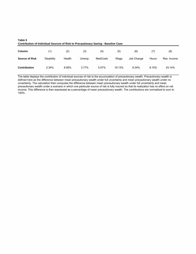
Table 5Contribution of Individual Sources of Risk to Precautionary Saving - Baseline Case

Column (1) (2) (3) (4) (5) (6) (7) (8)

Source of Risk Disability Health Unemp. MedCosts Wage Job Change Hours Res. Income

Contribution

The table displays the contribution of individual sources of risk to the accumulation of precautionary wealth. Precautionary wealth is defined here as the difference between mean precautionary wealth under full uncertainty and mean precautionary wealth under no uncertainty. The calculation then computes the difference between mean precautionary wealth under full uncertainty and mean precautionary wealth under a scenario in which one particular source of risk is fully insured so that its realization has no effect on net income. This difference is then expressed as a percentage of mean precautionary wealth. The contributions are normalized to sum to 100%.

2.34% 8.56% 3.77% 5.57% 19.13% 9.34% 8.15% 43.14%

Table 6Average Lifetime Earnings RegressionDependent Variable: (Simulated) Average Lifetime Earnings

Variable cons ζD (ζD)2 (ζD)3 ζH (ζH)2 μ μ2 μ3 η η2 pwT (pw

T)2 (pw

T)3 DT HT ET μ*pw

T

Estimate 3.358 -0.003 -0.016 -0.006 -0.015 -0.007 0.357 -0.038 0.005 0.149 -0.007 0.240 0.008 -0.018 -0.108 0.000 -0.040 -0.011SE (0.004) (0.001) (0.001) (0.000) (0.001) (0.001) (0.002) (0.001) (0.000) (0.001) (0.001) (0.004) (0.005) (0.004) (0.005) (0.003) (0.004) (0.004)

Obs. 48,030Root MSE 0.184Adj R-squared 0.88

212

The table presents estimation results for the average lifetime earnings regression. The regression uses data simulated from a joint model of labor earnings to determine the predictive power of variables known in the last year of a worker's career for his/her average lifetime earnings, as calculated by the Social Security Administration (taking, for instance, only the 35 years with highest earnings to calculate the average). The dependent variable is simulated average lifetime earnings. The independent variables are all permanent variables variables in the joint model of earnings, all time-varying variables in the last year of career only (year T), and some interactions. After experimentation with different specifications, only the interactions with a significant predictive power were included in the equation.

Table 7AWelfare Gains of Full Insurance: Sensitivity to Degree of Risk Aversion and Discount FactorEquivalent Variation in Lifetime Consumption - Effect Adjusted for Variation in Mean Income Profile (Actuarially Fair Insurance)

Disability Health Unemp. MedCosts Wage Job Change Hours Res.Income

Coefficient of Relative Risk Aversion

α = 3.0 0.02% 0.00% 0.04% 0.01% 1.20% 0.72% 0.45% 2.19%

α = 5.0 (1) 0.03% 0.01% 0.07% 0.02% 1.95% 1.17% 0.72% 4.79%

Discount Factor

β = 0.967 (2) 0.02% 0.00% 0.04% 0.01% 1.20% 0.72% 0.45% 2.19%

β = 0.94 (1) 0.01% 0.00% 0.05% 0.02% 0.97% 0.75% 0.44% 3.15%

β = 0.90 (1) 0.01% 0.00% 0.05% 0.02% 0.73% 0.77% 0.42% 4.19%

(1) All other parameters are held at their baseline value.(2) β = 1/(1+r).

Source of Risk

Panel (a)

Panel (b)

The table presents the welfare gains from fully insuring individual sources of risk (see Table 4.4A, Panel a) for different values of the coefficient of risk aversion α and the discount factor β.

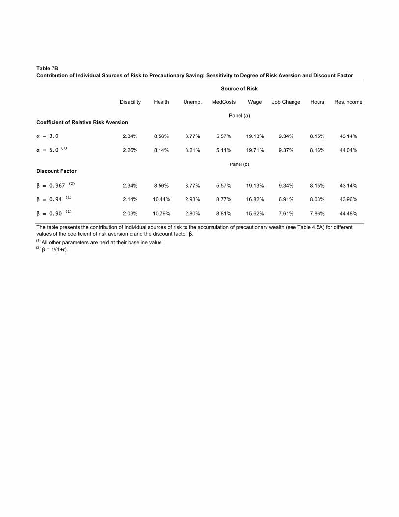
Table 7BContribution of Individual Sources of Risk to Precautionary Saving: Sensitivity to Degree of Risk Aversion and Discount Factor

Disability Health Unemp. MedCosts Wage Job Change Hours Res.Income

Coefficient of Relative Risk Aversion

α = 3.0 2.34% 8.56% 3.77% 5.57% 19.13% 9.34% 8.15% 43.14%

α = 5.0 (1) 2.26% 8.14% 3.21% 5.11% 19.71% 9.37% 8.16% 44.04%

Discount Factor

β = 0.967 (2) 2.34% 8.56% 3.77% 5.57% 19.13% 9.34% 8.15% 43.14%

β = 0.94 (1) 2.14% 10.44% 2.93% 8.77% 16.82% 6.91% 8.03% 43.96%

β = 0.90 (1) 2.03% 10.79% 2.80% 8.81% 15.62% 7.61% 7.86% 44.48%

(1) All other parameters are held at their baseline value.(2) β = 1/(1+r).

Source of Risk

Panel (a)

Panel (b)

The table presents the contribution of individual sources of risk to the accumulation of precautionary wealth (see Table 4.5A) for different values of the coefficient of risk aversion α and the discount factor β.

Figure 1

Mean Nonasset Income and Consumption by Potential Experience

05

1015202530354045

1 6 11 16 21 26 31 36 41 46 51 56 61 66

Potential Experience (years)

Thou

sand

s of

Yea

r-20

00 $

Income Consumption

The figure displays simulated mean nonasset income and simulated (optimal) mean consumption. The mean profiles are based on simulating the lifecycle model for 50,000 households. Period 43 is the exogenous retirement date. Income was parameterized such that income and consumption are measured in thousands of year-2000 dollars.

Figure 2

Optimal Consumption at t=1 by Cash on Hand

0

5

10

15

20

25

30

0 10 20 30 40 50 60 70 80 90 100

Cash on Hand in Thousands of Year-2000 $

Con

sum

ptio

n in

Tho

usan

ds o

fY

ear-2

000

$

The figure displays optimal consumption in the first period of career as a function of cash on hand for an employed, healthy individual with mean persistent wage and household income components. The figure corresponds to the baseline model, in which individuals face credit constraints.

Figure 3

Optimal Consumption at t=1 by Cash on Hand and Persistent Household Income Component

0

5

10

15

20

25

0 10 20 30 40 50 60Cash on Hand in Thousands of Year-2000 $

Con

sum

ptio

n in

Tho

usan

ds o

fYe

ar-2

000

$

The figure displays optimal consumption in the first period of career as a function of cash on hand for different levels of the persistent household income component, for an employed, healthy individual with mean (persistent) wage. The figure corresponds to the baseline model, in which individuals face credit constraints.

Figure 4

Optimal Consumption at t=1 by Cash on Hand and Persistent Wage

0

5

10

15

20

25

30

35

40

0 10 20 30 40 50 60 70 80 90 100

Cash on Hand in Thousands of Year-2000 $

Con

sum

ptio

n in

Tho

usan

ds o

fY

ear-2

000

$

The figure displays optimal consumption in the first period of career as a function of cash on hand for different levels of the persistent wage component, for an employed, healthy individual with mean persistent household income component. The figure corresponds to the baseline model, in which individuals face credit constraints.

Figure 5 Optimal Consumption at t=1 by Cash on Hand and Persistent Wage

(for wider range of values of persistent wage)

The figure displays optimal consumption in the first period of career as a function of the two continuous state variables in the numerical solution to the household consumption problem: cash on hand and the persistent wage. The figure refers to an employed individual in good health and with mean persistent household income component. It corresponds to the baseline model, in which individuals face credit constraints.

Figure 6

Mean Asset Holdings by Potential Experience

0

50

100

150

200

250

300

350

1 6 11 16 21 26 31 36 41 46 51 56 61 66

Potential Experience (years)

Thou

sand

s of

Yea

r-200

0 $

Full UncertaintyNo Uncertainty

The figure displays the mean level of assets held by households in simulations of the lifecycle model. The curve above represents mean asset holdings under the full-uncertainty scenario, while the curve below displays mean asset holdings under no uncertainty. The mean profile of net income is identical under both scenarios.

Figure 7

Mean Precautionary Wealth by Potential Experience

0

5

10

15

20

25

30

35

1 6 11 16 21 26 31 36 41 46 51 56 61 66

Potential Experience (years)

Thou

sand

s of

Yea

r-20

00 $

The figure displays mean precautionary wealth by year in the lifecycle. The figures are based on a simulation of a large cross-section of households. Mean precautionary wealth is the difference in mean asset holdings between the full-uncertainty scenario and the no-uncertainty scenario in which net income follows its mean profile deterministically.

Figure 8

Ratio of Precautionary Wealth to Total Wealth by Potential Experience

0.00

0.20

0.40

0.60

0.80

1.00

1.20

1 6 11 16 21 26 31 36 41 46 51 56 61 66

Potential Experience (years)

Rat

io

The figure displays the ratio of mean precautionary wealth to mean total wealth by year in the lifecycle. The figure is based on simulation of a large cross-section of households. Mean total wealth is the mean of asset holdings under the full-uncertainty world. Mean precautionary wealth is the difference in mean asset holdings between the full-uncertainty scenario and the no-uncertainty scenario in which net income follows its mean profile deterministically.