HAL Id: hal-00843150https://hal.archives-ouvertes.fr/hal-00843150

Preprint submitted on 10 Jul 2013

HAL is a multi-disciplinary open accessarchive for the deposit and dissemination of sci-entific research documents, whether they are pub-lished or not. The documents may come fromteaching and research institutions in France orabroad, or from public or private research centers.

L’archive ouverte pluridisciplinaire HAL, estdestinée au dépôt et à la diffusion de documentsscientifiques de niveau recherche, publiés ou non,émanant des établissements d’enseignement et derecherche français ou étrangers, des laboratoirespublics ou privés.

Precautionary Saving over the Business CycleEdouard Challe, Xavier Ragot

To cite this version:

Edouard Challe, Xavier Ragot. Precautionary Saving over the Business Cycle. 2013. hal-00843150

PRECAUTIONARY SAVING OVER THE BUSINESS CYCLE

Edouard CHALLE Xavier RAGOT

July 2013

Cahier n° 2013-15

ECOLE POLYTECHNIQUE CENTRE NATIONAL DE LA RECHERCHE SCIENTIFIQUE

DEPARTEMENT D'ECONOMIE Route de Saclay

91128 PALAISEAU CEDEX (33) 1 69333033

http://www.economie.polytechnique.edu/ mailto:chantal.poujouly@polytechnique.edu

Precautionary Saving over the Business Cycle∗

Edouard Challe† Xavier Ragot‡

February 5, 2013

Abstract

We study the macroeconomic implications of time-varying precautionary saving

within a general equilibrium model with borrowing constraint and both aggregate shocks

and uninsurable idiosyncratic unemployement risk. Our framework generates limited

cross-sectional household heterogeneity as an equilibrium outcome, thereby making it

possible to analyse the role of precautionary saving over the business cycle in an ana-

lytically tractable way. The time-series behaviour of aggregate consumption generated

by our model is much closer to the data than that implied by the comparable hand-

to-mouth and representative-agent models, and comparable to that produced by the

(intractable) Krusell-Smith (1998) model. (JEL E20, E21, E32)

∗We are particularly grateful to Olivier Allais, Paul Beaudry, Hafedh Bouakez, Nicola Pavoni, Morten

Ravn, Sergio Rebelo and Pontus Rendahl for their detailed comments at various stages of this project. We

also greatly benefited from discussions with Yann Algan, Fernando Alvarez, Andrew Atkeson, Pierre Cahuc,

Christophe Chamley, Bernard Dumas, Emmanuel Farhi, Jonathan Heathcote, Christian Hellwig, Per Krusell,

Etienne Lehmann, Julien Matheron, Benoit Mojon, Franck Portier, Ricardo Reis, José-Víctor Ríos Rull, Kjetil

Storesletten, Philippe Weil and Ivan Werning. We also thank conference participants to the 2012 Hydra

Workshop on Dynamic Macroeconomics, the EABCN/CEPR Conference on Disaggregating the Business

Cycle, the 2012 ASSA Meetings, the 2011 SED Congress, the 2011 NBER Summer Institute, the 2011 Paris

Macro Finance Workshop, the 2010 Minnesota Workshop in Macroeconomic Theory, the 2010 Philadelphia Fed

Search and Matching Workshop, as well as seminar participants at Ecole Polytechnique, Sciences Po, EIEF,

LBS, INSEAD, HEC Paris, HEC Lausanne, ECB, Banque de France, Bank of Portugal, Gains/Université du

Mans, Aix-Marseille School of Economics, Stockholm University (IIES), Tilburg University and the University

of Cambridge. Eric Mengus provided outstanding research assistance, and the French Agence Nationale pour

la Recherche (grant no 06JCJC0157) and chaire FDIR provided funding. The usual disclaimers apply.†CNRS (UMR 7176), Ecole Polytechnique, CREST and Banque de France. Email:

edouard.challe@polytechnique.edu.‡CNRS (UMR 8545) and Paris School of Economics. Email: ragot@pse.ens.fr.

1

1 Introduction

Although precautionary saving against uninsurable income shocks has been widely analysed

theoretically and empirically, it has remained diffi cult to incorporate into dynamic general

equilibrium models for at least two reasons. First, the lack of full insurance usually produces

a considerable amount of agent heterogeneity, essentially because the wealth of any particular

agent —and, by way of consequence, the decisions it makes—generally depends on the entirely

history of income shocks that this agent has faced (see, e.g., Huggett, 1993; Aiyagari, 1994;

Guerrieri and Lorenzoni, 2011). Second, aggregate shocks turn the cross-sectional distribution

of wealth into a time-varying state variable, the evolution of which every agent must forecast

in order to make their best intertemporal decisions. In their pioneering contribution, Krusell

and Smith (1998) have proposed a solution to this problem, which consists in simplifying the

agents’s forecasting problem by approximating the full cross-sectional distribution of wealth

with a small number of moments. However, the lack of tractability of the underlying problem

makes their solution method operational only in relatively simple environments; in particular,

both the number of state variables and the support for the exogenous shocks must remain

limited.1

In this paper, we construct a class of heterogenous-agent models with incomplete markets,

borrowing constraints and both aggregate and idiosyncratic labour income shocks than can be

solved under exact cross-household aggregation and rational expectations. More specifically,

we exhibit a set of suffi cient conditions about preferences and the tightness of the borrowing

constraint, under which the model endogenously generates a cross-sectional distribution of

wealth with a limited number of states; exact aggregation directly follows. This approach

makes it possible to derive analytical results and incorporate time-varying precautionary

saving into general equilibrium analysis using simple solution methods —including linearisation

and undetermined coeffi cient methods. In particular, our analysis allows the derivation of a

common asset-holding rule for employed households facing incomplete insurance, possibly

expressed in linear form, which explicitly connects precautionary wealth accumulation to

the risk of experiencing an unemployment spell.2 Additionally, our model can be simulated

1Krusell et al. (2010, p. 1497) refer to this approach as one in which “consumers have boundedly rational

perceptions of the evolution of the aggregate state”. As mentioned there, the approach is valid under the

conjecture that “approximate aggregation”holds, so that the forecasting rules used by the agents take the

economy close to the true rational-expectations equilibrium. See Heathcote et al. (2010) for a discussion of

this point and Algan et al. (2010) for a survey of alternative computational algorithms.2Since a substantial fraction of the households does not achieve full self-insurance in equilibrium (despite

2

with several —and possibly imperfectly correlated—aggregate shocks with continuous support;

we consider three such shocks in our baseline specification (i.e., technology, job-finding and

job-separation shocks).

In order to isolate, both theoretically and quantitatively, the precautionary motive in

the determination of households’savings, our general framework incorporates both patient,

“permanent-income” consumers and impatient consumers who are imperfectly insured and

may face occasionally binding borrowing constraints. Aside from the baseline precautionary-

saving case just discussed, wherein impatient households hold a time-varying buffer-stock

of wealth in excess of the borrowing limit, our framework also nests two special cases of

interest: the representative-agent model and the hand-to-mouth model. The representative-

agent model arises as a limit of our incomplete-market model when the economy becomes

entirely populated by permanent-income consumers. The hand-to-mouth model —a situation

when impatient households face a binding borrowing limit in every period— endogenously

arises when the precautionary motive becomes too weak to offset impatience, so that impatient

agents end up consuming their entire income in every period.3 We trace back the strength

of the precautionary motive —and thus whether or not impatient households are ultimately

willing to save—analytically to the deep parameter of the model, most notably the extent of

unemployment risk, the generosity of the unemployment insurance scheme, and the tightness

of the borrowing constraint.

We then use our framework to identify and quantify the specific role of incomplete insur-

ance and precautionary wealth accumulation —as opposed to, e.g., mere borrowing constraints—

in determining the volatility of aggregate consumption and its co-movements with output. To

this purpose, we calibrate the model so as to match the main features of the cross-sectional

distributions of wealth and nondurables consumption in the US economy —in addition to

matching other usual quantities. We then feed the calibrated model with aggregate shocks

to productivity and labour market transition rates with magnitude and joint behaviour that

are directly estimated from post-war US data. We find the time-series behaviour of aggregate

precautionary wealth accumulation), they experiences a discontinuous drop in income and consumption when

unemployment strikes. This drop being of first-order magnitude, changes in the perceived likelihood that it will

occur have a correspondingly first-order impact on the intensity of the precautionary motive for accumulating

assets ex ante.3In this case, our economy collapses to a two-agent one of the kind studied by, e.g., Becker and Foias

(1987), Kiyotaki and Moore (1997), or Iacoviello (2005). We refer to this situation as the “hand-to-mouth”

case even when the borrowing limit is not strictly zero —since agents then end up consuming their entire

income, including their negative capital income.

3

consumption generated by our baseline precautionary-saving model to be much closer to the

data than those implied by the comparable hand-to-mouth and representative-agent models.

Perhaps unsurprisingly, the representative-agent limit of our framework generates to little

consumption volatility and too low a consumption-output correlation. More interestingly, the

comparable hand-to-mouth model generates not only too high a consumption-output corre-

lation (due to constrained households’consumption tracking their income), but also too little

consumption volatility. By contrast, the precautionary-saving model generates a much higher

level of consumption volatility, because consumption then responds to expected labour-market

conditions (via the precautionary motive) in addition to current labour market conditions

(the key determinant of consumption in the hand-to-mouth case). Time-varying precaution-

ary saving also contributes to relax the tight output-consumption association predicted by

the hand-to-mouth case, without taking it to a level as low as in the representative-agent

case. To complete the picture, we also compare the moments of interest implied by our

baseline precautionary-saving model with those generated by the full-fledged heterogenous-

agent model of Krusell and Smith (1998, Section IV). Despite their structural differences,

the Krusell-Smith model and our baseline incomplete-market model predict similar levels of

consumption volatility and consumption-output correlation —and those most in line with the

data relative to the alternative specifications.

Our analysis differs from earlier attempts at constructing tractable models with incomplete

markets, which typically restrict the stochastic processes for the idiosyncratic shocks in ways

that makes them ill-suited for the analysis of time-varying unemployment risk. For example,

Constantinides and Duffi e (1996) study the asset-pricing implications of an economy in which

households are hit by repeated permanent income shocks. This approach has been generalised

by Heathcote et al. (2008) to the case where households’income is affected by insurable tran-

sitory shocks, in addition to imperfectly insured permanent shocks. Toche (2005), and more

recently Carroll and Toche (2011) explicitly solve for households’optimal asset-holding rule

in a partial-equilibrium economy where they face the risk of permanently exiting the labour

market. Guerrieri and Lorenzoni (2009) analyse precautionary saving behaviour in a model

with trading frictions a la Lagos and Wright (2005), and show that agents’liquidity hoard-

ing amplify the impact of i.i.d. (aggregate and idiosyncratic) productivity shocks. Relative

to these models, ours allows for stochastic transitions across labour market statuses, which

implies that individual income shocks are transitory (but persistent) and have a conditional

distribution that depends on the aggregate state. The model is thus fully consistent with the

flow approach to the labour market and can be evaluated using direct evidence on the cyclical

4

movements in labour market transition rates.4

The remainder of the paper is organised as follows. The following section introduces

the model. It starts by describing households’consumption-saving decisions in the face of

idiosyncratic unemployment risk; it then spells out firms’optimality conditions and charac-

terises the equilibrium. In Section 3, we introduce the parameter restrictions that make our

model tractable by endogenously limiting the dimensionality of the cross-sectional distrib-

ution of wealth. Section 4 calibrates the model and compares its quantitative implications

to the data, as well as to three alternative benchmarks —the representative-agent model, the

hand-to-mouth model and the Krusell-Smith model. Section 6 concludes.

2 The model

The model features a closed economy populated by a continuum of households indexed by i and

uniformly distributed along the unit interval, as well as a representative firm. All households

rent out labour and capital to the firm, which latter produces the unique (all-purpose) good

in the economy. Markets are competitive but there are frictions in the financial markets, as

we describe further below.

2.1 Households

Every household i is endowed with one unit of labour, which is supplied inelastically to the

representative firm if the household is employed.5 All households are subject to idiosyn-

cratic changes in their labour market status between “employment” and “unemployment”.

Employed households earn a competitive market wage (net of social contributions), while

unemployed households earn a fixed unemployment benefit δi > 0.6

4Carroll (1992), and more recently Parker and Preston (2005) have suggested that changes in precautionary

wealth accumulation following (countercyclical) changes in the extent of unemployment risk significantly

amplify aggregate consumption fluctuations. This motivates our focus on idiosyncratic and time-varying

unemployment risk as a driver of aggregate savings, a focus that we share with Krusell and Smith (1998).5Our model ignores changes in hours worked per employed workers, since those play a relatively minor role

in the cyclical component of total hours in the US (see, e.g., Rogerson and Shimer, 2011). Incorporating an

elastic labour supply for employed workers would be a simple extensions of our baseline specification.6Following much of the heterogenous-agent literature, we focus on (un)employemnt risk as the main source

of idiosyncratic income fluctuations at business-cycle frequency. Our model could easily be extended to

introduce wage risk in addition to employment risk (as in, e.g., Low et al. (2010)).

5

We assume that households can be of two types, impatient and patient, with the former

and the latter having subjective discount factors βI ∈ (0, 1) and βP ∈(βI , 1

)and occu-

pying the subinterval [0,Ω] and (Ω, 1], respectively, where Ω ∈ [0, 1). While not necessary

for the construction of our equilibrium with limited cross-sectional heterogeneity below, the

introduction of patient households will allow us to generate a substantial degree of cross-

sectional wealth dispersion, since patient households will end up holding a large fraction of

total wealth in equilibrium.7 However, in contrast to models featuring heterogenous discount

factors wherein impatient households face a binding borrowing limit and hence behave like

mere “hand-to-mouth”consumers8, most of the impatient in our baseline model will hold a

wealth buffer in excess of the borrowing limit —and will thus not face a binding constraint.

As we shall see in Section 4 below, that these households do not behave as hand-to-mouth

consumers crucially matters for the aggregate time-series properties of the model.

Unemployment risk. The unemployment risk faced by individual households is sum-

marised by two probabilities: The probability that a household who is employed at date

t − 1 becomes unemployed at date t (the job-loss probability st), and the probability that a

household who is unemployed at date t − 1 stays so at date t (i.e., 1 − ft, where ft is the

job-finding probability). The law of motion for employment is9

nt = (1− nt−1) ft + (1− st)nt−1. (1)

One typically thinks of cyclical fluctuations in (ft, st) as being ultimately driven by more

fundamental shocks governing the job creation policy of the firms and the natural breakdown

of existing employment relationships. For example, endogenous variations in (ft, st) naturally

arise in a labour market plagued by search frictions, wherein both transition rates are affected

by the underlying productivity shocks. We provide a model of such a frictional labour market

in Appendix A.10 However, we wish to emphasise here that the key market friction leading

7Krusell and Smith (1998) introduced heterogenous, stochastic discount factors to generate plausible levels

of wealth dispersion in their incomplete-market environement. Our specification is closer to that in McKay

and Reis (2012) who use heterogenous, but deterministic, discount factors.8See, e.g., Becker (1980); Becker and Foias (1987); Kiyotaki and Moore (1997); Iacoviello (2005).9This formulation is fully constitent with the possibility of unemployment spells shorter than a period

(e.g., a quarter). Assume, for example, that an employed worker at the end of date t− 1 looses its job at the

beginning of date t with probability ρt, but is re-hired during the same period with probability ft. Then, the

period-to-period job-loss probability is st = ρt (1− ft), while the employment dynamics (1) still holds.10See also Krusell et al. (2011), who solve numerically a full-fledged heterogenous-agent model with incom-

plete insurance and labour market frictions.

6

to time-varying precautionary savings is the inability of some households to perfectly insure

against such transitions, a property that does not depend on the specific modelling of the

labour market being adopted. For this reason, we take those transition rates as exogenous in

our baseline specification, and will ultimately extract them from the data in the quantitative

implementation of the model.

Impatient households. Impatient households maximise their expected life-time utility

E0

∑∞t=0

(βI)tuI (cit), i ∈ [0,Ω], where cit is (nondurables) consumption by household i at date

t and uI(.) a period utility function satisfying uI′ (.) > 0 and uI′′ (.) ≤ 0. We restrict the

set of assets that impatient households have access to in two ways. First, we assume that

they cannot issue assets contingent on their employment status but only enjoy the (partial)

insurance provided by the public unemployment insurance scheme; and second, we assume

that these households face an (exogenous) borrowing limit in that their asset wealth cannot fall

below −µ, where µ ≥ 0.11 Given these restrictions, the only asset that can be used to smooth

out idiosyncratic labour income fluctuations are claims to the capital stock. We denote by eit

household’s i employment status at date t, with eit = 1 if the household is employed and zero

otherwise. The budget and non-negativity constraints faced by an impatient household i are:

ait + cit = eitwIt (1− τt) +

(1− eit

)δI +Rta

it−1, (2)

cit ≥ 0, ait ≥ −µ. (3)

where ait is household i’s holdings of claims to the capital stock at the end of date t, Rt the

ex post gross return on these claims, wIt the real wage for impatient households (assumed to

be identical across them), δI the unemployment benefit enjoyed by these households when

unemployed, and wIt τt a contribution paid by the employed and aimed at financing the un-

employment insurance scheme.12 The Euler condition for impatient households is:

uI′(cit)

= βIEt(uI′(cit+1

)Rt+1

)+ ϕit, (4)

11In our model, this constraint will effectively binds only for the households who are both impatient and

unemployed, a small fraction of the population (3.4% in our baseline calibration). The model can accomodate

an endogenous borrowing limit based on limited commitment, e.g., if households pleageable income is a

constant fraction µ of next period’s expected future labour income. This does not significantly affect our

results provided that pledgeable income is not too volatile. See Guerrieri and Lorenzoni (2011) for an analysis

of how an exogenous change in the tightness of the constraint (as arguably occurred at the oneset of the Great

Recession) affects outcomes under incomplete markets.12Since households do not choose hours or participation here, it does not matter for aggregate dynamics

whether social contributions are proportional or lump sum.

7

where ϕit is the Lagrange coeffi cient associated with the borrowing constraint ait ≥ 0, with

ϕit > 0 if the constraint is binding and ϕit = 0 otherwise. Condition (4), together with

the initial asset holdings ai−1 and the terminal condition limt→∞Et[βItaitu

I′ (cit)] = 0, fully

characterise the optimal asset holdings of impatient households.

Patient households. Patient households maximise E0

∑∞t=0

(βP)tuP (cit), i ∈ (Ω, 1] , where

βP ∈(βI , 1

)and uP (.) is increasing and strictly concave over [0,∞). In contrast to impatient

households, patient households have complete access to asset markets —including the full set

of Arrow-Debreu securities and loan contracts.13 Full insurance implies that these households

collectively behave like a large representative ‘family’ of permanent-income consumers in

which the family head ensures equal marginal utility of wealth for all its members —despite

the fact that individuals experience heterogenous employment histories (see, e.g., Merz, 1995;

Hall, 2009). Since consumption is the only argument in the period utility, equal marginal

utility of wealth implies equal consumption, so we may write the budget constraint of the

family as follows:

CPt + APt = RtA

Pt−1 + (1− Ω)

(ntw

Pt (1− τt) + (1− nt) δP

), (5)

where CPt (≥ 0) andAPt denote the consumption and end-of-period asset holdings of the family

(both of which must be divided by 1− Ω to find the per-family member analogues), and wPt

and δP are the real wage and unemployment benefit for patient households, respectively. The

Euler condition for patient households is given by:

uP ′(

CPt

1− Ω

)= βPEt

(uP ′(CPt+1

1− Ω

)Rt+1

). (6)

This condition, together with the initial asset holdings AP−1 and the terminal condition

limt→∞Et[(βP)tAPt u

P ′ (CPt / (1− Ω)

)] = 0, fully characterise the optimal consumption path

of patient households. Note that when Ω = 0 then only fully-insured patient households

populate the economy, and the latter become a representative-agent economy.13Patient households will be more wealthy than impatient households in equilibrium —and a lot more so

when we calibrate the model to match the cross-sectional distribution of wealth in the US. Under fixed

participation cost to trading Arrow-Debreu securities (as in, e.g., Mengus and Pancrasi (2012)), we expect

households holding more wealth (patient households here) to be more willing to buy insurance, all else equal.

From a quantitative point of view, Krusell and Smith (1998) have argued that the behaviour of wealthy agents

facing incomplete markets and borrowing constraints is almost undistinguishable from that of fully insured

agents. Finally, it is easy to show that in our economy the borrowing constraint would never be binding

for fully-insured patient households in equilibrium, even if such a constraint were assumed in the first place

(because patient households are relatively wealthy and claims to the capital stock are in positive net supply).

8

2.2 Production

The representative firm produces output, Yt, out of capital, Kt, and the units of effective

labour supplied by the households. Let nIt and nPt denote the firm’s use of impatient and

patient households’ labour input, respectively, and Yt = ztG(Kt, n

It + κnPt

)the aggregate

production function, where κ > 0 is the relative effi ciency of patient households’ labour

(with the effi ciency of impatient households’labour normalised to one), zt∞t=0 a stochastic

aggregate productivity process with unconditional mean z∗ = 1, and where G (., .) exhibits

positive, decreasing marginal products and constant returns to scale (CRS). As will be clear in

Section 4 below, the introduction of an effi ciency premium for patient households (i.e., κ > 1),

which raises their labour income share in equilibrium relative to the symmetric case (κ = 1),

is necessary to match the cross-sectional consumption dispersion, for any plausible level of

wealth dispersion.14 Defining kt ≡ Kt/(nIt + κnPt

)as capital per unit of effective labour

and g (kt) ≡ G (kt, 1) the corresponding intensive-form production function, we have Yt =

zt(nIt + κnPt

)g (kt). Capital depreciates at the constant rate ν ∈ [0, 1], so that investment is

It ≡ Kt+1−(1− ν)Kt. Given Rt and zt, the optimal demand for capital by the representative

firm satisfies:

ztg′ (kt) = Rt − 1 + ν. (7)

On the other hand, the optimal demands for the two labour types in a perfectly competitive

labour market must satisfy ztG2

(Kt, n

It + κnPt

)= wIt = wPt /κ, where w

It is the real wage per

unit of effective labour.

2.3 Market clearing

By the law of large numbers and the fact that all households face identical transition rates

in the labour market, the equilibrium numbers of impatient and patient households working

in the representative firm are nIt = Ωnt and nPt = (1− Ω)nt, respectively. Consequently,

effective labour and capital are nIt + κnPt = (Ω + (1− Ω)κ)nt (with nt given by (1)) and

14Although we do not model it explicitly here, that κ > 1 is a direct implication of standard human capital

accumulation models, which predict that more patient agents accumulate more human capital in the first place

(e.g., Ben Porath, 1967). Our underlying assumption of perfect substituability between effi cient labour units

is made for simplicity, as it makes the equilibrium wage premium wPt /wIt constant and equal to the exogenous

productivity premium κ. Introducing imperfect substituabilty between labour types (see, e.g., Acemoglu and

Autor, 2011) makes the wage premium a function of the employment levels (nPt , nIt ) but does not alter the

basic mechanisms that we focus on.

9

Kt = (Ω + (1− Ω)κ)ntkt, respectively. Moreover, by the CRS assumption the equilibrium

real wage per unit of effective labour is wIt = zt (g (kt)− ktg′ (kt)).In general, we expect incomplete insurance against unemployment shocks to generate

cross-sectional wealth dispersion, as the asset wealth accumulated by a particular household

depends on the employment history of this household. We summarise this heterogeneity in

accumulated wealth by Ft (a, e) , which denotes the measure at date t of impatient households

with beginning-of-period asset wealth a and employment status e, and we denote by at (a, e)

and ct (a, e) the corresponding policy functions for assets and consumption.15 Since those

households are in share Ω in the economy, clearing of the market for claims to the capital

stock requires that

APt−1 + Ω∑e=0,1

∫ +∞

a=−µat−1 (a, e) dFt−1 (a, e) = (Ω + (1− Ω)κ)ntkt, (8)

where the left hand side of (8) is total asset holdings by all households at the end of date t−1

and the right hand side the demand for capital by the representative firm at date t. Clearing

of the goods market requires:

CPt + Ω

∑e=0,1

∫ +∞

a=−µct (a, e) dFt (a, e) + It = zt (Ω + (1− Ω)κ)ntg (kt) , (9)

where the left hand side of (9) includes the consumption of all households as well as aggregate

investment, It = (Ω + (1− Ω)κ) (nt+1kt+1 − (1− ν)ntkt) , and the right hand side is output.

Finally, we require the unemployment insurance scheme to be balanced, i.e.,

τtnt(ΩwIt + (1− Ω)wPt

)= (1− nt)

(ΩδI + (1− Ω) δP

), (10)

where the left and right hand sides of (10) are total unemployment contributions and benefits,

respectively.

An equilibrium of this economy is defined as a sequence of households’decisions CPt , c

it,

APt , ait∞t=0, i ∈ [0,Ω], firm’s capital per effective labour unit kt∞t=0, and aggregate vari-

ables nt, wIt , Rt, τt∞t=0, which satisfy the households’and the representative firm’s optimality

conditions (4), (6) and (7), together with the market-clearing and balanced-budget condi-

tions (8)—(10), given the forcing sequences ft, st, zt∞t=0 and the initial wealth distribution(Ap−1, a

i−1,)i∈[0,Ω]

.

15Our formulation of the market-clearing conditions (8)—(9) presumes the existence of a recursive formulation

of the household’s problem with (a, e) as individual state variables, as this will be the case in the equilibrium

that we are considering. See, e.g., Heathcote (2005) for a nonrecursive formulation of the household’s problem.

10

3 An equilibrium with limited cross-sectional hetero-

geneity

As is well known, dynamic general equilibrium models with incomplete markets and borrow-

ing constraints are not tractable, essentially because any household’s decisions depend on

its accumulated asset wealth, while the latter is determined by the entire history of idiosyn-

cratic shocks that this household has faced. In consequence, the asymptotic cross-sectional

distribution of wealth usually has an infinitely large number of states, and hence infinitely

many agent types end up populating the economy (Aiyagari, 1994; Krusell and Smith, 1998).

In this paper, we make specific assumptions about impatient household’s period utility and

the tightness of the borrowing constraint, which ensure that the cross-sectional distribution

of wealth has a finite number of wealth states as an equilibrium outcome. As a result, the

economy is characterised by a finite number of heterogenous agents whose behaviour can

be aggregated exactly, thereby making it possible to represent the model’s dynamics via a

standard (small-scale) dynamic system. In the remainder of the paper, we focus on the sim-

plest equilibrium, which involves exactly two possible wealth states for impatient households.

However, we show in Section 3.3 and Appendix B how this approach can be generalised to

construct equilibria with any finite number of wealth states.

3.1 Assumptions and conjectured equilibrium

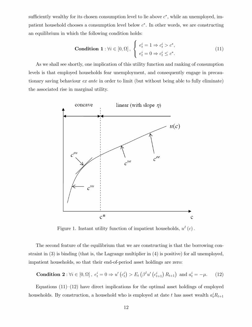
Let us first assume that the instant utility function for impatient households uI (c) is i) con-

tinuous, increasing and differentiable over [0,+∞) , ii) strictly concave with local relative

risk aversion coeffi cient σI (c) = −cuI′′ (c) /uI′ (c) > 0 over [0, c∗], where c∗ is an exogenous,

positive threshold, and iii) linear with slope η > 0 over (c∗,+∞) (see Figure 2). Essen-

tially, this utility function (an extreme form of decreasing relative risk aversion) implies that

high-consumption (i.e., relatively wealthy) impatient households do not mind moderate con-

sumption fluctuations —i.e., as long as the implied optimal consumption level says inside

(c∗,+∞)—but dislike substantial consumption drops —those that would cause consumption to

fall inside the [0, c∗] interval.

Given this utility function, we derive our equilibrium with limited cross-sectional hetero-

geneity by construction; Namely, we first guess the general form of the solution, and then

verify ex post that the set of conditions under which the conjectured equilibrium was derived

does prevail in equilibrium. Our first conjecture is that an employed, impatient household is

11

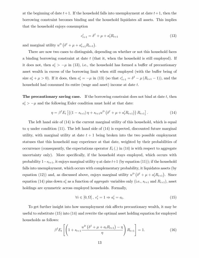
suffi ciently wealthy for its chosen consumption level to lie above c∗, while an unemployed, im-

patient household chooses a consumption level below c∗. In other words, we are constructing

an equilibrium in which the following condition holds:

Condition 1 : ∀i ∈ [0,Ω] ,

eit = 1⇒ cit > c∗,

eit = 0⇒ cit ≤ c∗.(11)

As we shall see shortly, one implication of this utility function and ranking of consumption

levels is that employed households fear unemployment, and consequently engage in precau-

tionary saving behaviour ex ante in order to limit (but without being able to fully eliminate)

the associated rise in marginal utility.

Figure 1. Instant utility function of impatient households, uI (c) .

The second feature of the equilibrium that we are constructing is that the borrowing con-

straint in (3) is binding (that is, the Lagrange multiplier in (4) is positive) for all unemployed,

impatient households, so that their end-of-period asset holdings are zero:

Condition 2 : ∀i ∈ [0,Ω] , eit = 0⇒ u′(cit)> Et

(βIu′

(cit+1

)Rt+1

)and ait = −µ. (12)

Equations (11)—(12) have direct implications for the optimal asset holdings of employed

households. By construction, a household who is employed at date t has asset wealth aitRt+1

12

at the beginning of date t+1. If the household falls into unemployment at date t+1, then the

borrowing constraint becomes binding and the household liquidates all assets. This implies

that the household enjoys consumption

cit+1 = δI + µ+ aitRt+1 (13)

and marginal utility uI′(δI + µ+ ait+1Rt+1

).

There are now two cases to distinguish, depending on whether or not this household faces

a binding borrowing constraint at date t (that it, when the household is still employed). If

it does not, then ait > −µ in (13), i.e., the household has formed a buffer of precautionaryasset wealth in excess of the borrowing limit when still employed (with the buffer being of

size ait + µ > 0). If it does, then ait = −µ in (13) (so that cit+1 = δI − µ (Rt+1 − 1)), and the

household had consumed its entire (wage and asset) income at date t.

The precautionary saving case. If the borrowing constraint does not bind at date t, then

ait > −µ and the following Euler condition must hold at that date:

η = βIEt[(

(1− st+1) η + st+1uI′ (δI + µ+ aitRt+1

))Rt+1

]. (14)

The left hand side of (14) is the current marginal utility of this household, which is equal

to η under condition (11). The left hand side of (14) is expected, discounted future marginal

utility, with marginal utility at date t + 1 being broken into the two possible employment

statuses that this household may experience at that date, weighted by their probabilities of

occurrence (consequently, the expectations operator Et (.) in (14) is with respect to aggregate

uncertainty only). More specifically, if the household stays employed, which occurs with

probability 1−st+1, it enjoys marginal utility η at date t+1 (by equation (11)); if the household

falls into unemployment, which occurs with complementary probability, it liquidates assets (by

equation (12)) and, as discussed above, enjoys marginal utility uI′(δI + µ+ aitRt+1

). Since

equation (14) pins down ait as a function of aggregate variables only (i.e., st+1 and Rt+1), asset

holdings are symmetric across employed households. Formally,

∀i ∈ [0,Ω] , eit = 1⇒ ait = at. (15)

To get further insight into how unemployment risk affects precautionary wealth, it may be

useful to substitute (15) into (14) and rewrite the optimal asset holding equation for employed

households as follows:

βIEt

[(1 + st+1

uI′(δI + µ+ atRt+1

)− η

η

)Rt+1

]= 1. (16)

13

Consider, for the sake of the argument, the effect of a fully predictable increase in st+1

holding Rt+1 constant. The direct effect is to raise 1 + st+1[uI′(δI + µ+ atRt+1

)− η]/η,

since the proportional change in marginal utility associated with becoming unemployed,

[uI′(δI + µ+ atRt+1

)− η]/η, is positive (see Figure 1). Hence, uI′

(δI + µ+ atRt+1

)must

go down for (16) to hold, which is achieved by raising date t asset holdings, at. Later on we

derive an approximate asset holding rule that explicitly connects current precautionary asset

wealth to the expected job-loss rate and the expected interest rate.

The hand-to-mouth case. In the case where the borrowing constraint is binding for em-

ployed, impatient households —in addition to being binding for the unemployed, as conjectured

in (12)—, then from (2) the consumption of employed households is wt (1− τt) − µ (Rt − 1)

while that of unemployed households is δI − µ (Rt − 1). In other words, all impatient house-

holds consume their entire (wage and asset) income in every period. Our model thus nests

the pure “hand-to-mouth” behaviour as a special case, which occurs when the borrowing

constraint is binding for all impatient households (and not only the unemployed). As we

discuss below, this corner scenario notably arises when i) direct unemployment insurance is

suffi ciently generous (so that self-insurance is deterred), or impatient households’discount

factor is suffi ciently low (i.e., households are too impatient to save).

Aggregation. The analysis above implies that, under conditions (11)—(12), the cross-sectional

distribution of wealth amongst impatient households at any point in time has at most two

states: exactly two (−µ and at > −µ) if the borrowing constraint is binding for unemployedhouseholds but not for employed households, and exactly one (−µ) if the constraint is binding

for all impatient households, employed and unemployed alike. This in turn implies that the

economy is populated by at most four types of impatient households —since from (2) the type

of a household depends on both beginning- and end-of-period asset wealth. We call these

types ‘ij’, i, j = e, u, where i (j) refers to the household’s employment status in the previous

(current) date (for example, a ‘ue household’is currently employed but was unemployed in

the previous period, and its consumption at date t is cuet ). These consumption levels are :

ceet = wt (1− τt) +Rtat−1 − at, (17)

ceut = δI + µ+Rtat−1, (18)

cuet = wt (1− τt)− at − µRt, (19)

cuut = δI + µ− µRt. (20)

14

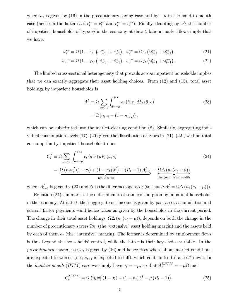
where at is given by (16) in the precautionary-saving case and by −µ in the hand-to-mouthcase (hence in the latter case ceet = cuet and ceut = cuut ). Finally, denoting by ω

ij the number

of impatient households of type ij in the economy at date t, labour market flows imply that

we have:

ωeet = Ω (1− st)(ωeet−1 + ωuet−1

), ωeut = Ωst

(ωeet−1 + ωuet−1

), (21)

ωuut = Ω (1− ft)(ωeut−1 + ωuut−1

), ωuet = Ωft

(ωeut−1 + ωuut−1

). (22)

The limited cross-sectional heterogeneity that prevails across impatient households implies

that we can exactly aggregate their asset holding choices. From (12) and (15), total asset

holdings by impatient households is

AIt ≡ Ω∑e=0,1

∫ +∞

a=−µat (a, e) dFt (a, e) (23)

= Ω (ntat − (1− nt)µ) ,

which can be substituted into the market-clearing condition (8). Similarly, aggregating indi-

vidual consumption levels (17)—(20) given the distribution of types in (21)—(22), we find total

consumption by impatient households to be:

CIt ≡ Ω

∑e=0,1

∫ +∞

a=−µct (a, e) dFt (a, e) (24)

= Ω(ntw

It (1− τt) + (1− nt) δI

)+ (Rt − 1)AIt−1︸ ︷︷ ︸

net income

− Ω∆ (nt (at + µ))︸ ︷︷ ︸change in asset wealth

,

where AIt−1 is given by (23) and∆ is the difference operator (so that ∆AIt = Ω∆ (nt (at + µ))).

Equation (24) summarises the determinants of total consumption by impatient households

in the economy. At date t, their aggregate net income is given by past asset accumulation and

current factor payments —and hence taken as given by the households in the current period.

The change in their total asset holdings, Ω∆ (nt (at + µ)), depends on both the change in the

number of precautionary savers Ωnt (the “extensive”asset holding margin) and the assets held

by each of them at (the “intensive”margin). The former is determined by employment flows

is thus beyond the households’control, while the latter is their key choice variable. In the

precautionary saving case, at is given by (16) and hence rises when labour market conditions

are expected to worsen (i.e., st+1 is expected to fall), which contributes to take CIt down. In

the hand-to-mouth (HTM ) case we simply have at = −µ, so that AI,HTMt = −µΩ and

CI,HTMt = Ω

(ntw

It (1− τt) + (1− nt) δI − µ (Rt − 1)

), (25)

15

implying that only current labour market conditions affect CI,HTMt (via their effect on nt).

Comparing (24) and (25), we get that:

CIt = CI,HTM

t + Ω (Rtnt−1 (at−1 + µ)− nt (at + µ)) .

The latter expression shows how total consumption by impatient households —and, by

way of consequence, aggregate consumption itself—differs across the hand-to-mouth and the

precautionary-saving cases. In the hand-to-mouth case, only current labour market conditions

nt —in addition to factor prices (wIt , Rt)—affect total consumption by impatient households.

In the precautionary-saving case, the same effects are at work but, in addition, future labour

market conditions matter —inasmuch as they affect at. This suggests that the precautionary

saving model may display more consumption volatility than the hand-to-mouth model, pro-

vided that labour market conditions are suffi ciently persistent. This will be confirmed in the

quantitative analysis of Section 4 below.

3.2 Existence conditions and steady state

Existence conditions. The equilibriumwith limited cross-sectional heterogeneity described

so far exists provided that two conditions are satisfied. First, the postulated ranking of con-

sumption levels for impatient households in (11) must hold in equilibrium. Second, unem-

ployed, impatient households must face a binding borrowing constraint (see (12)).

• From (17)—(20) and the fact that at ≥ −µ (with equality in the hand-to-mouth case),we have cuut ≤ ceut and ceet ≥ cuet . Hence, a necessary and suffi cient condition for (11) to

hold is ceut < c∗ < cuet , that is,

δI + µ+ at−1Rt < c∗ < wIt (1− τt)− at − µRt. (26)

• Unemployed, impatient households can be of two types, uu and eu, and we require bothtypes to face a binding borrowing constraint in equilibrium. However, since cuut ≤ ceut

(and hence uI′ (cuut ) ≥ uI′ (ceut )), a necessary and suffi cient condition for both types to

be constrained is

uI′ (ceut ) > βIEt((ft+1u

I′ (cuet ) + (1− ft+1)uI′(cuut+1

))Rt+1),

where the right hand side of the inequality is the expected, discounted marginal utility

of an eu household who is contemplating the possibility of either remaining unemployed

(with probability 1−ft+1) or finding a job (with probability ft+1). Under the conjectured

16

equilibrium we have uI′ (cuet ) = η and cuut+1 = δI + µ (1−Rt+1), so the latter inequality

becomes:

uI′(δI + µ+ at−1Rt

)> βIEt

((ft+1η + (1− ft+1)uI′

(δI + µ (1−Rt+1)

))Rt+1

). (27)

In what follows, we compute the steady state of our conjectured equilibrium and derive

a set of necessary and suffi cient conditions for (26)—(27) to hold in the absence of aggregate

shocks. By continuity, they will also hold in the stochastic equilibrium provided that the

magnitude of aggregate shocks is not too large.

Steady state. In the steady state, the real interest rate is determined by the discount rate

of the most patient households, so that R∗ = 1/βP (see (6)). From (1) and (7), the steady

state levels of employment and capital per effective labour unit are

n∗ =f ∗

f ∗ + s∗, k∗ = g′−1

(1

βP− 1 + ν

). (28)

A key variable in the model is the level of asset holdings that employed, impatient house-

holds hold as a buffer against unemployment risk. If the borrowing constraint is binding

in the steady state, then they never hold wealth. The interior solution to the steady state

counterpart of (16) (where R∗ = 1/βP ) gives the individual asset holdings:

a∗ = βP[uI′−1

(η

(1 +

βP − βIβIs∗

))− δI − µ

]. (29)

The borrowing constraint is binding whenever the interior solution a∗ in (29) is less than

−µ. Hence the actual steady-state wealth level of employed, impatient households is givenby:

a∗ = max [−µ, a∗] , (30)

which nests both the precautionary-saving and hand-to-mouth cases discussed above.

Equations (29)—(30) are informative about the conditions under which the economy col-

lapses to a hand-to-mouth economy. More specifically, employed, impatient households form

no buffer stock of wealth whenever a∗ < −µ, that is, using (29)—(30) and rearranging, when-ever

βP − βIβI

> s∗ ×u′(δI + µ− µ/βP

)− η

η. (31)

This inequality is straightforward to interpret. In the hand-to-mouth case, the steady state

consumption level of an impatient household who is transiting into unemployment is δI +µ−µ/βP —that is, the unemployment benefit δI plus new borrowing µ minus the debt repayment

17

µ at the gross interest rate 1/βP . Thus, the right hand side of (31) is the proportional cost —in

terms of marginal utility—associated with a completely unbuffered transition from employment

(where marginal utility is η) to unemployment (where marginal utility is u′(δI + µ− µ/βP

)),

weighted by the probability of this transition occuring (the job-loss probability s∗). The

higher the probability of this transition, the stronger the incentive to buffer the shock and

the less likely (31) will hold, all else equal. Conversely, the higher the unemployment benefit

δI , the lower the actual cost of the transition when it occurs, the weaker the incentive to

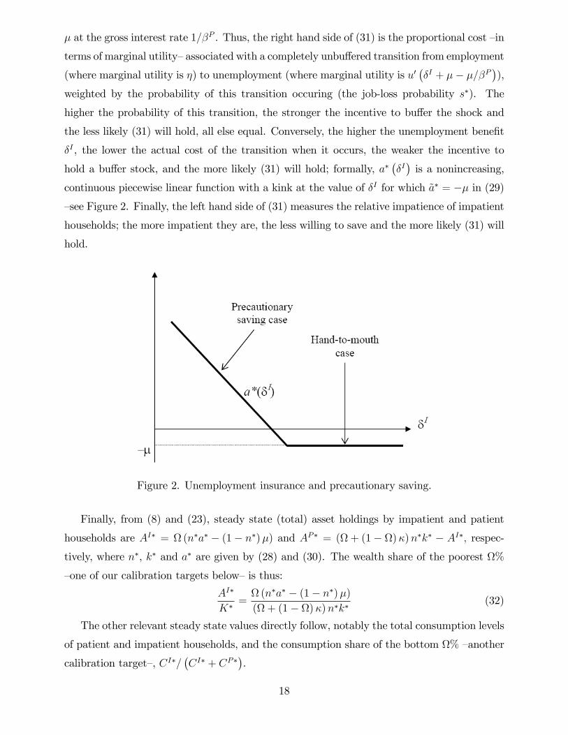
hold a buffer stock, and the more likely (31) will hold; formally, a∗(δI)is a nonincreasing,

continuous piecewise linear function with a kink at the value of δI for which a∗ = −µ in (29)—see Figure 2. Finally, the left hand side of (31) measures the relative impatience of impatient

households; the more impatient they are, the less willing to save and the more likely (31) will

hold.

Figure 2. Unemployment insurance and precautionary saving.

Finally, from (8) and (23), steady state (total) asset holdings by impatient and patient

households are AI∗ = Ω (n∗a∗ − (1− n∗)µ) and AP∗ = (Ω + (1− Ω)κ)n∗k∗ − AI∗, respec-

tively, where n∗, k∗ and a∗ are given by (28) and (30). The wealth share of the poorest Ω%

—one of our calibration targets below—is thus:

AI∗

K∗=

Ω (n∗a∗ − (1− n∗)µ)

(Ω + (1− Ω)κ)n∗k∗(32)

The other relevant steady state values directly follow, notably the total consumption levels

of patient and impatient households, and the consumption share of the bottom Ω% —another

calibration target—, CI∗/(CI∗ + CP∗).

18

We may now state the following proposition, which establishes the conditions on the deep

parameters of the model under which a steady state with limited cross-sectional heterogeneity

exists. Provided that aggregate shocks have suffi ciently small magnitude, the same conditions

will ensure the existence of a stochastic equilibrium with similarly limited heterogeneity.

Proposition 1. Assume that i) there are no aggregate shocks, ii) unemployment insurance

is incomplete (i.e., δI < wI∗ (1− τ ∗)) and iii) the following inequality holds:

η

(1 +

βP − βIβIs∗

)>

max

[βI

βP

(fη + (1− f)u′

(δI − µ

(1

βP− 1

))), u′(wI∗ (1− τ ∗) + βP δI

1 + βP− µ

(1

βP− 1

))],

where

τ ∗ =

(1− n∗n∗

)ΩδI + (1− Ω) δP

(Ω + (1− Ω)κ)wI∗, (33)

wI∗ = g (k∗)− k∗g′ (k∗) , and (n∗, k∗) are given by (28). Then, it is always possible to find a

utility threshold c∗ such that the conjectured limited-heterogeneity equilibrium described above

exists. In this equilibrium, a∗ = −µ (a∗ > −µ) if (31) holds (does not hold).

Proof. First, the steady state counterpart of (27) is

a∗ < βPuI′−1

[βI

βP

(fη + (1− f)u′

(δI + µ

(βP − 1

βP

)))]− βP

(δI + µ

). (34)

Second, the steady state counterpart of (26) is δI + µ+ a∗/βP < c∗ < wI∗ (1− τt)− a∗ −µ/βP . A suffi cient condition for the existence of a threshold c∗ is thus that δI + µ+ a∗/βP <

wI∗ (1− τt)− a∗ − µ/βP , or

a∗ <βPΓ

1 + βP− µ, (35)

where Γ ≡ wI∗ (1− τ ∗) − δI = (1− τ ∗) [g (k∗)− k∗g′ (k∗)] − δI is a strictly positive constantthat only depends on the deep parameters of the model (see (28) and (33)). Inequalities

(34)—(35) hold for a∗ = −µ (the hand-to-mouth case). Otherwise, a∗ is given by (29) (theprecautionary saving case); substituting this value of a∗ into (34)—(35) and rearranging gives

the inequality in the proposition

The inequalities in Proposition 1 ensure that, in the steady state, i. the candidate equi-

librium features at most two possible wealth levels for impatient households (−µ for theunemployed and a∗ ≥ −µ for the employed); and ii. the implied ranking of individual con-sumption levels is indeed such that we can “reverse-engineer”an instant utility function for

19

these households of the form depicted in Figure 1. Those inequalities can straightforwardly be

checked once specific values are assigned to the deep parameters of the model. As we argue in

Section 4 below, it is satisfied for plausible such values when we calibrate the model to the US

economy. The reason for which it does is as follows. Our limited-heterogeneity equilibrium

requires that impatient, unemployed households be borrowing-constrained (i.e., they would

like to borrow against future income but are prevented from doing so), while impatient, em-

ployed households accumulate suffi ciently little wealth in equilibrium (so that this wealth be

exhausted within a quarter of unemployment). In the US, the quarter-to-quarter probability

of leaving unemployment is high and the replacement ratio relatively low, leading the unem-

ployed’s expected income to be suffi ciently larger than current income for these households

to be willing to borrow. On the other hand, the US distribution of wealth is fairly unequal,

leading a large fraction of the population (the impatient in our model) to hold a very small

fraction of total wealth.

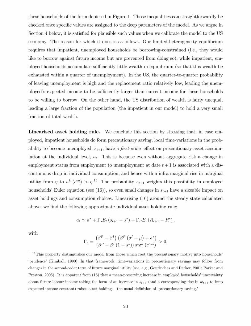
Linearised asset holding rule. We conclude this section by stressing that, in case em-

ployed, impatient households do form precautionary saving, local time-variations in the prob-

ability to become unemployed, st+1, have a first-order effect on precautionary asset accumu-

lation at the individual level, at. This is because even without aggregate risk a change in

employment status from employment to unemployment at date t+ 1 is associated with a dis-

continuous drop in individual consumption, and hence with a infra-marginal rise in marginal

utility from η to uI′ (ceu) > η.16 The probability st+1 weights this possibility in employed

households’Euler equation (see (16)), so even small changes in st+1 have a sizeable impact on

asset holdings and consumption choices. Linearising (16) around the steady state calculated

above, we find the following approximate individual asset holding rule:

at ' a∗ + ΓsEt (st+1 − s∗) + ΓREt (Rt+1 −R∗) ,

with

Γs =

(βP − βI

) (βP(δI + µ

)+ a∗

)(βP − βI (1− s∗)) s∗σI (ceu∗)

> 0,

16This property distinguishes our model from those which root the precautionary motive into households’

‘prudence’ (Kimball, 1990). In that framework, time-variations in precautionary savings may follow from

changes in the second-order term of future marginal utility (see, e.g., Gourinchas and Parker, 2001; Parker and

Preston, 2005). It is apparent from (16) that a mean-preserving increase in employed households’uncertainty

about future labour income taking the form of an increase in st+1 (and a corresponding rise in wt+1 to keep

expected income constant) raises asset holdings —the usual definition of ‘precautionary saving.’

20

and where a∗ is given by (29), ceu∗ = δI + µ + a∗R∗ is the steady state counterpart of (18),

and σI (ceu∗) ≡ −ceu∗uI′′ (ceu∗) /uI′ (ceu∗) is the coeffi cient of relative risk aversion of impatienthouseholds evaluated at ceu∗ (i.e., the steady state consumption level of a household falling

into unemployment). The composite parameter Γs measures the strength of the response of

individuals’precautionary wealth following predicted changes in unemployment risk, such as

summarised by the period-to-period separation rate st+1.17

3.3 Equilibria with multiple wealth states

In the previous sections, we have constructed an equilibrium with limited cross-sectional

heterogeneity characterised by the simplest (nondegenerate) distribution of wealth, that with

two states. A key feature of this equilibrium is that impatient households face a binding

borrowing constraint after the first period of unemployment —and hence liquidate their entire

asset wealth. As we argue next, instant asset liquidation by wealth-poor households is a

natural outcome of our framework when we calibrate it on a quarterly basis and using US

data on the cross-sectional distribution of wealth. However, we emphasise that the same

approach can be use to construct equilibria with any finite number of wealth states, wherein

households gradually, rather than instantly, sell assets to offset their individual income fall.

We carefully derive in Appendix B a set of necessary and suffi cient conditions for the

existence and uniqueness of limited-heterogeneity equilibria with m + 1 wealth states (that

is, m strictly positive wealth states), thereby generalising the constructive approach used in

Sections 3.1—3.2. As before, we focus on those conditions at the steady state, and resort to

perturbation arguments to extend them to the stochastic equilibrium. An equilibrium with

m + 1 wealth states has the property that the only impatient households facing a binding

borrowing constraint are those having experienced at least m consecutive periods of unem-

ployment. Before the mth unemployment period, the asset wealth and consumption level of

these households decreases gradually. From the m+ 1th unemployment period, these house-

holds face a binding borrowing constraint, hold no wealth, and have a flat consumption path.

Finally, we show that an equilibrium with m + 1 wealth states is associated with 2 (m+ 1)

types of impatient households (that is, the cross-sectional distribution of consumption has

2 (m+ 1) possible states).

To see this intuitively how this gradual process of asset decumulation can occur in our17ΓR may be positive or negative depending on the relative strengths of the intertemporal income and

substitution effects. In particular, high values of σI produce asset accumulation rules that prescribe an

increase in at following a fall in Et (Rt+1) .

21

framework, consider for simplicity the case where µ = 0 and consider the steady state of the

simple equilibrium described above and take its existence condition with respect to the bind-

ingness of the borrowing constraint for an impatient households who fall into unemployment:

uI′(δI + a∗R∗

)> βI

[(ηf ∗ + (1− f ∗)uI′

(δI))R∗], (36)

where δI+a∗R∗ is the consumption of those households under full liquidation, η their marginal

utility in the next period if they exit unemployment, and δI their consumption in the next

period if they stay unemployed (with no assets left, by construction).

The circumstances leading to the violation of inequality (36), so that the equilibrium with

two wealth states described above no longer exists, are the following. First, the job-finding

rate f ∗ or the unemployment benefit δI may be too low, leading to high marginal utility

in the next period (the right hand side of (36)), thereby urging the household to transfer

wealth into the future. Second, the asset holdings accumulated when employed (a∗, which is

itself determined by (29)) may be too high, leading to low current marginal utility (the left

hand side (36)), thereby making this transfer little costly to the household. However, even if

inequality (36) is violated for one of these reasons, a similar condition might nevertheless hold

for households having experienced two consecutive periods of unemployment, because those

have less wealth (and hence higher current marginal utility) than in the first unemployment

period. In this case, the equilibrium will have exactly three wealth states (including two

strictly positive), rather than two.

4 Time-varying precautionary saving and consumption

fluctuations

The model developed above implies that some households rationally respond to countercyclical

changes in unemployment risk by raising precautionary wealth —and thus by cutting down

individual consumption more than they would have done without the precautionary motive.

We now wish to assess the extent of this effect on aggregate consumption when realistic

unemployment shocks are fed into our model economy. To this purpose, we compute the

response of aggregate consumption and output to aggregate shocks implied by our baseline

model, and then compare it with the data as well as a number of comparable benchmarks

including i. the hand-to-mouth model, ii. the representative-agent economy, and iii. Krusell

& Smith (1998) “stochastic-beta”economy.

22

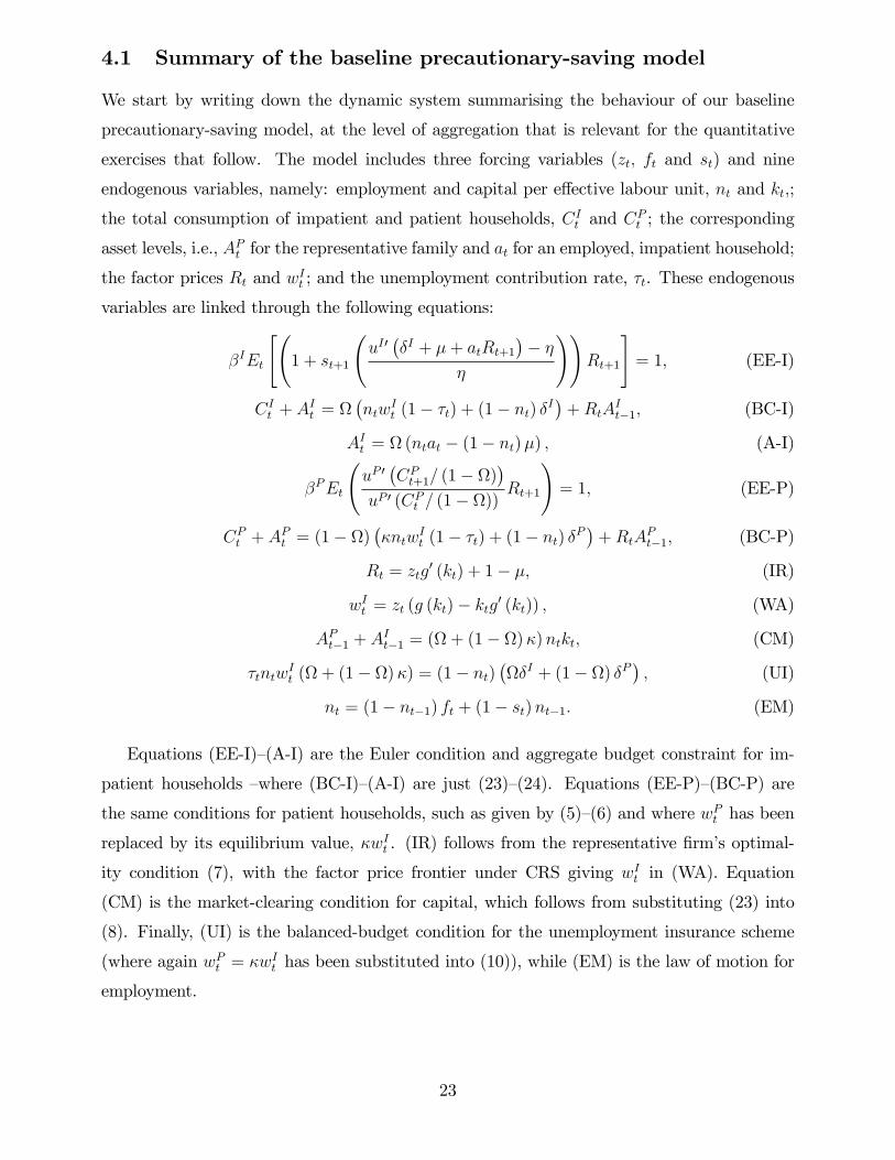
4.1 Summary of the baseline precautionary-saving model

We start by writing down the dynamic system summarising the behaviour of our baseline

precautionary-saving model, at the level of aggregation that is relevant for the quantitative

exercises that follow. The model includes three forcing variables (zt, ft and st) and nine

endogenous variables, namely: employment and capital per effective labour unit, nt and kt,;

the total consumption of impatient and patient households, CIt and C

Pt ; the corresponding

asset levels, i.e., APt for the representative family and at for an employed, impatient household;

the factor prices Rt and wIt ; and the unemployment contribution rate, τt. These endogenous

variables are linked through the following equations:

βIEt

[(1 + st+1

(uI′(δI + µ+ atRt+1

)− η

η

))Rt+1

]= 1, (EE-I)

CIt + AIt = Ω

(ntw

It (1− τt) + (1− nt) δI

)+RtA

It−1, (BC-I)

AIt = Ω (ntat − (1− nt)µ) , (A-I)

βPEt

(uP ′(CPt+1/ (1− Ω)

)uP ′ (CP

t / (1− Ω))Rt+1

)= 1, (EE-P)

CPt + APt = (1− Ω)

(κntw

It (1− τt) + (1− nt) δP

)+RtA

Pt−1, (BC-P)

Rt = ztg′ (kt) + 1− µ, (IR)

wIt = zt (g (kt)− ktg′ (kt)) , (WA)

APt−1 + AIt−1 = (Ω + (1− Ω)κ)ntkt, (CM)

τtntwIt (Ω + (1− Ω)κ) = (1− nt)

(ΩδI + (1− Ω) δP

), (UI)

nt = (1− nt−1) ft + (1− st)nt−1. (EM)

Equations (EE-I)—(A-I) are the Euler condition and aggregate budget constraint for im-

patient households —where (BC-I)—(A-I) are just (23)—(24). Equations (EE-P)—(BC-P) are

the same conditions for patient households, such as given by (5)—(6) and where wPt has been

replaced by its equilibrium value, κwIt . (IR) follows from the representative firm’s optimal-

ity condition (7), with the factor price frontier under CRS giving wIt in (WA). Equation

(CM) is the market-clearing condition for capital, which follows from substituting (23) into

(8). Finally, (UI) is the balanced-budget condition for the unemployment insurance scheme

(where again wPt = κwIt has been substituted into (10)), while (EM) is the law of motion for

employment.

23

4.2 Alternative benchmarks

In what follows, we shall compare the time-series properties of our baseline precautionary

saving model with the following alternative benchmarks.

Hand-to-mouth model. As discussed in Section 3, the hand-to-mouth model arises en-

dogenously as a particular case of our framework whenever (31) holds (and aggregate shocks

have suffi ciently small magnitude). In this equilibrium all impatient households face a binding

borrowing constraint in every period, so that at = −µ for all t. The dynamics of the hand-to-mouth model is obtained by removing equation (EE-I) from the dynamic system (EE-I)-(EM)

above and by imposing at = −µ in equation (A-I).

Representative-agent model. Our framework also nests the representative-agent model

as a special case. The comparable representative-economy is obtained by setting ΩRA = 0

—so that all households are identical and perfectly insured—and κRA = Ω + (1− Ω)κ —so that

average labour productivity is kept the same as in the baseline precautionary-saving model.

The subjective discount factor βP is kept at the same value as in the baseline model, so that

the steady state interest factor R∗ = 1/βP , and hence capital per effective labour unit k∗,

are unchanged. Since steady-state total wealth is (Ω + (1− Ω)κ)n∗k∗ (see (8)), it takes the

same value in the representative-agent model as in the baseline precautionary-saving model

(and also the hand-to-mouth model).

Krusell-Smith model. We also compare the quantitative implications of our model with

the stochastic-beta version of the Krusell and Smith (1998) heterogenous-agent model. We

thus simulate exactly the same model and then compute the moments that we wish to com-

pare to those implied by our baseline model with limited cross-sectional heterogeneity.18 Our

motivation for focusing on the stochastic-beta version of the model is twofold. First, it incor-

porates discount factor heterogeneity which, as our model, potentially generates a substantial

amount of cross-sectional wealth dispertion (as is usually observed empirically, notably in the

US). Second, the stochastic-beta model is the Krusell-Smith variant that differs most from the

full-insurance model in term of the consumption-output correlation, one of the key moments

we are also interested in (see Table 2 in Krusell and Smith, 1998).

18We refer the reader to their paper for the description of their model and results (and notably Section 4

for the stochastic-beta model).

24

4.3 Calibration

We set the time period to a quarter (and thus allow unemployment spells to be shorter than

a period —see footnote 7), and calibrate the model so that its steady state matches some key

features of the cross-sectional distributions of wealth and consumption in the US economy

(see Table 1 below). We then simulate the model to infer its its time-series properties under

this calibration as well as alternative specification (as summarised in Table 2).

Idiosyncratic risk and insurance The extent of idiosyncratic risk that households face

is measured by the labour market transition rates (f ∗, s∗ at the steady state), while the

degree of insurance that they enjoy depends on both the replacement ratio δI/w∗I and the

borrowing limit µ. The steady state values of f ∗ and s∗ are set to their quarter-to-quarter

post-war averages (see Appendix C for how quarterly series for ft and st are constructed). By

construction, these values produce a steady-state unemployment rate s∗/(f ∗ + s∗) also equal

to its post-war average, 5.65%.

In a narrow sense, the gross replacement ratio δj/w∗j, j = I, P, measures the replacement

income provided by the unemployment insurance scheme and should thus be set between 0.4

and 0.5 for the US (see, e.g., Shimer, 2005; Chetty, 2008). However, households also benefit

from other, nonobservable sources of insurance —family, friends etc.—We take this into account

by calibrating δj/w∗j so as to generate a plausible level of consumption insurance. Cochrane

(1991) argues that the average nondurable consumption growth of consumers experiencing

an involuntary job loss is 25 percentage point lower than those who do not. Gruber (1997)

focuses on the impact of UI benefits on the size of the consumption fall of households having

experienced a job loss, and find a significantly smaller number —about 7 percent. We set our

baseline gross replacement ratio δj/w∗j to 0.6 (rather than, say, 0.5) which, together with

the other parameters of the model, produces a consumption growth differential of 14.08% for

the average households;19 we also evaluate the impact of a larger replacement ratio in our

sensitivity experiments.

In the model, only the households who are both impatient —and hence have little assets in

the first place—and unemployed face a binding borrowing constraint. In our baseline scenario,

19Patient households are fully insured and hence experience noconsumption fall when falling into unem-

ployemnt. Hence, the average proportional consumption drop associated with falling into unemployment is

Ω (ce∗ − ceu∗) /ce∗, where ce∗ ≡ f∗ (1− n∗) cue∗ + (1− s)n∗cee∗ is the average consumption of and employed,impatient households. Our calibrated replacement ratio being perfectly symmetric across households, we are

implicitly ignoring the potential redistributive effects of the unemployemnt insurance scheme.

25

we simply assume that these househoulds cannot borrow (i.e., µ = 0), and then evaluate the

impact of a relaxation of this constraint in our sensitivity analysis.20 As we shall see, relaxing

the borrowing within a plausible range significantly affects the cross-sectional distribution of

wealth but not the time-series implications of the model.

Preferences. On the households’side, we adopt the following baseline parameters. We set

the share of impatient households, Ω, to 0.6 (and experiment with an alternative value of

0.3 in our sensitivity analysis); since only a fraction 1− n∗ of such households face a bindingborrowing constraint in the baseline precautionary-saving model, and given the calibrated

steady-state transition rates f ∗ and s∗ (see above), this implies a steady-state share of ef-

fectively borrowing-constrained households of Ω (1− n∗) = 3.4%.21 The discount factor of

patient household, βP (= 1/R∗), is set to 0.99, and their instant utility to uP (c) = ln c.

The utility function of impatient households is set to

uI (c) =

ln c for c ≤ 1.6

ln 1.6 + 0.486 (c− 1.6) for c > 1.6,

which satisfies the assumptions in Section 2.1 (with η = 0.486 and c∗ = 1.6). The chosen value

of η is equal to the steady state marginal utility of ee households (by far the most numerous

amongst the impatient) if they had the same instant utility function as patient households —

given the other parameters—, and is meant to minimise differences in asset holding behaviour

purely due to differences in instant utility functions.22 Note that uI (c) is continuous and

(weakly) concave but not differentiable all over [0,∞) (since uI′ (1.6) > 0.486); however, it

can be made so by ‘smooth pasting’the two portions of the function in an arbitrarily small

neighbourhood of c∗ while preserving concavity. We set the discount factor of impatient

households, βI , to match the wealth share of the Ω% poorest households, given the other

parameters including βP . We focus on nonhome (or “liquid”) wealth, since our analysis

20Sullivan (2008) finds the response of (unsecured) individual debt to unemployment shocks to be inexistent

or very small (a tenth of the associated income loss) in the US.21Model with “rule-of-thumb”consumers usually have a larger fraction of effectively constrained households,

ranging from 15% to 60% (see, e.g., Campbell and Mankiw, 1989; Iacoviello, 2005; Gali et al., 2007; Mertens

and Ravn, 2011; Kaplan and Violante, 2012). In the hand-to-mouth economy, the share of effectively con-

strained household is raised from (1− n∗) Ω (= 3.4%) to Ω (= 60%) (since all impatient households, including

the employed, are then constrained).22More specifically, η solves η = uP ′ (cee∗) =

(wI∗ + a∗

(1− 1/βP

))−1. This equation indicates that the

appropriate value of η depends on a∗. Since a∗ also depends on η (by (29)), we jointly solve for the fixed

point (a∗, η) using a iterative procedure.

26

pertains to the the part of households’net worth that can readily be converted into cash to

provide for current (nondurables) consumption. A value of βI = 0.9697 produces a wealth

share of 0.30% for the 60% poorest households (the AI∗/K∗ ratio in (32)), which matches the

corresponding quantile of the distribution of nonhome wealth in the 2007 Survey of Consumer

Finances (see Wolff, 2011, Table 2).23

Technology. On the production side, we assume a Cobb-Douglas production function

Yt = ztKαt

(nIt + κnPt

)1−α, with α = 1/3, and a depreciation rate ν = 2.5%. The produc-

tivity premium parameter κ on patient households’labour is set to 1.731. Since impatient

households’ productivity is normalised to 1, this implies an equilibrium skill premium of

73.1%). Given the other parameters (see below), this will produce a consumption share

CI∗/(CI∗+CP∗) of 40.62% for the 60% poorest households, which exactly matches the cross-

sectional distribution of nondurables in the 2009 Consumer Expenditure Survey.24 Note that

this value is also well in line with the direct evidence on the level of the skill premium such

as reported in, e.g., Heathcote et al. (2010) or Acemoglu and Autor (2011).

Our baseline parameterisation is summarised in Table 1. Given those parameters, and

in particular the implied low wealth share of impatient households, the existence conditions

summarised in Proposition 1 are satisfied (by a large margin). In particular, households who

fall into unemployment without enjoying full insurance exhaust their buffer stock of wealth

within a quarter, and thus live entirely out of unemployment benefits thereafter. Given the

baseline values of Ω and κ, the representative-agent economy (i.e., in which ΩRA = 0) must be

parametrised with a skill premium parameter κRA = Ω+(1− Ω)κ = 0.6+0.4×1.731 = 1.292.

Finally, from (31) the calibrated model becomes a hand-to-mouth model whenever the steady

state gross replacement ratio for impatient households, δI/wI∗, exceeds 0.694.

23According to Gruber (1998), the mean probability of selling one’s home for those who become unemployed

is only 3% —that is, households typically do not sell their home to smooth nondurables consumption. Besides

the net ownership of the primary residence, the nonhome wealth distribution reported in Wolff (2011) excludes

consumer durables (whose resale value is low) as well as the social security and pension components of wealth

(which cannot be marketed). See Wolff (2011) for a full discussion of this point.24Our empirical couterpart for the consumption share of impatient households is the share of nondurables

consumed by the bottom three quintiles of households in terms of pre-tax income, where we define nondurables

as in Heathcote et al. (2010).

27

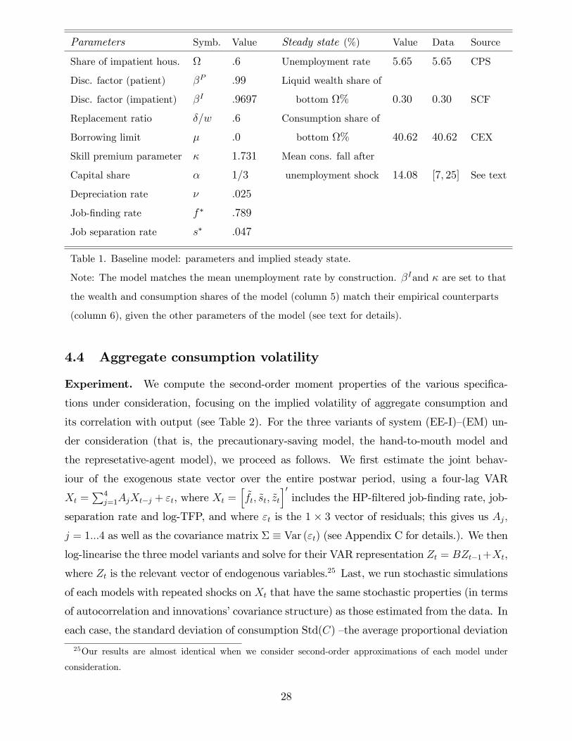
Parameters Symb. Value Steady state (%) Value Data Source

Share of impatient hous. Ω .6 Unemployment rate 5.65 5.65 CPS

Disc. factor (patient) βP .99 Liquid wealth share of

Disc. factor (impatient) βI .9697 bottom Ω% 0.30 0.30 SCF

Replacement ratio δ/w .6 Consumption share of

Borrowing limit µ .0 bottom Ω% 40.62 40.62 CEX

Skill premium parameter κ 1.731 Mean cons. fall after

Capital share α 1/3 unemployment shock 14.08 [7, 25] See text

Depreciation rate ν .025

Job-finding rate f ∗ .789

Job separation rate s∗ .047

Table 1. Baseline model: parameters and implied steady state.

Note: The model matches the mean unemployment rate by construction. βIand κ are set to that

the wealth and consumption shares of the model (column 5) match their empirical counterparts

(column 6), given the other parameters of the model (see text for details).

4.4 Aggregate consumption volatility

Experiment. We compute the second-order moment properties of the various specifica-

tions under consideration, focusing on the implied volatility of aggregate consumption and

its correlation with output (see Table 2). For the three variants of system (EE-I)—(EM) un-

der consideration (that is, the precautionary-saving model, the hand-to-mouth model and

the represetative-agent model), we proceed as follows. We first estimate the joint behav-

iour of the exogenous state vector over the entire postwar period, using a four-lag VAR

Xt =∑4

j=1AjXt−j + εt, where Xt =[ft, st, zt

]′includes the HP-filtered job-finding rate, job-

separation rate and log-TFP, and where εt is the 1 × 3 vector of residuals; this gives us Aj,

j = 1...4 as well as the covariance matrix Σ ≡ Var (εt) (see Appendix C for details.). We then

log-linearise the three model variants and solve for their VAR representation Zt = BZt−1 +Xt,

where Zt is the relevant vector of endogenous variables.25 Last, we run stochastic simulations

of each models with repeated shocks on Xt that have the same stochastic properties (in terms

of autocorrelation and innovations’covariance structure) as those estimated from the data. In

each case, the standard deviation of consumption Std(C) —the average proportional deviation

25Our results are almost identical when we consider second-order approximations of each model under

consideration.

28

from trend, in %—is computed, as well as its correlation with output, Corr(Yt, Ct).

As discussed above, we also compare these moments with those implied by the stochastic-

beta, Krusell and Smith (1998) model.26 Because that model is not tractable, it has a single,

two-state exogenous state variable which affects both total factor productivity and labour-

market transition rates. This is in contrast with the other three stochastic experiments

described above, which use a somewhat richer structure of aggregate shocks (namely, the

estimated joint behaviour of transition rates and total factor productivity). Since we are

simulating the same model, our value of Corr(Yt, Ct) in Table 2 below exactly replicates theirs

(see Krusell and Smith, 1998, Table 2, p. 886). We also compute the wealth share of the 60%

poorest as well as the standard deviation of aggregate consumption; in the later calculation,

the simulated consumption series is loged and HP-filtered (with smoothing parameter 1600)

before computing the standard deviation, so that the latter is comparable with those generated

by the other models (which are expressed in percent deviation from trend).

Results. The top part of Table 2 reports, for each model under consideration (Model 2 to

5), the wealth share of the poorest Ω% (in the baseline scenario where Ω = 0.6) as well as the

second-order moments under investigation, and compare them with the data (Row 1). The

bottom part of Table 2 carries out a number of sensitivity experiments around the baseline

precautionary-saving model

The two models that are closest to the data are the baseline precautionary-saving model

(Model 2) and the Krusell-Smith model (Model 4). As argued above, Model 2 has been

parameterised to match the empirical share of liquid wealth held by the poorest 60% —hence

the identity between the two in the Table (=0.30); in contrast, Model 4 was parameterised

by Krusell and Smith (1998, Section IV) to fit the Lorenz curve for net worth; since net

worth is less unequally distributed than liquid wealth, it generates a greater corresponding

wealth share than does Model 2. As is extensively discussed in Krusell and Smith (1998), the

wealth distribution in Model 4 implies that a large fraction of the households are reasonably

well self-insured against idiosyncratic shocks, implying that their behaviour is close to that

of pure permanent-income consumers; this shows up here as a smaller consumption volatility

generated by Model 4 relative to Model 2.

Perhaps unsurprisingly, the comparable representative-agent economy (Model 5) gener-

ates far too much consumption smoothing, which shows up here in the very low values of

both the standard deviation of aggregate consumption and its correlation with output. More

26We simulated 10 000 households for 11 000 periods and discarded the first 1 000 periods.

29

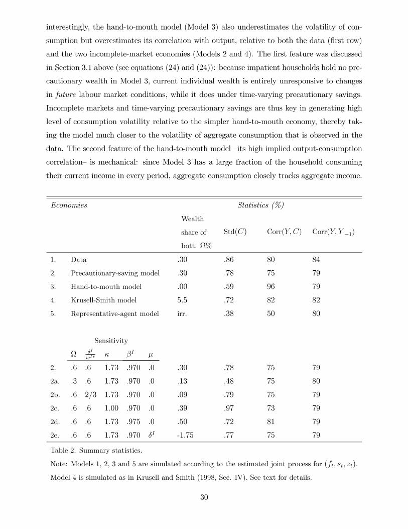
interestingly, the hand-to-mouth model (Model 3) also underestimates the volatility of con-

sumption but overestimates its correlation with output, relative to both the data (first row)

and the two incomplete-market economies (Models 2 and 4). The first feature was discussed

in Section 3.1 above (see equations (24) and (24)): because impatient households hold no pre-

cautionary wealth in Model 3, current individual wealth is entirely unresponsive to changes

in future labour market conditions, while it does under time-varying precautionary savings.

Incomplete markets and time-varying precautionary savings are thus key in generating high

level of consumption volatility relative to the simpler hand-to-mouth economy, thereby tak-

ing the model much closer to the volatility of aggregate consumption that is observed in the

data. The second feature of the hand-to-mouth model —its high implied output-consumption

correlation— is mechanical: since Model 3 has a large fraction of the household consuming

their current income in every period, aggregate consumption closely tracks aggregate income.

Economies Statistics (%)

Wealth

share of

bott. Ω%

Std(C) Corr(Y,C) Corr(Y, Y −1)

1. Data .30 .86 80 84

2. Precautionary-saving model .30 .78 75 79

3. Hand-to-mouth model .00 .59 96 79

4. Krusell-Smith model 5.5 .72 82 82

5. Representative-agent model irr. .38 50 80

Sensitivity

Ω δI

wI∗ κ βI µ

2. .6 .6 1.73 .970 .0 .30 .78 75 79

2a. .3 .6 1.73 .970 .0 .13 .48 75 80

2b. .6 2/3 1.73 .970 .0 .09 .79 75 79

2c. .6 .6 1.00 .970 .0 .39 .97 73 79

2d. .6 .6 1.73 .975 .0 .50 .72 81 79

2e. .6 .6 1.73 .970 δI -1.75 .77 75 79

Table 2. Summary statistics.

Note: Models 1, 2, 3 and 5 are simulated according to the estimated joint process for (ft, st, zt).

Model 4 is simulated as in Krusell and Smith (1998, Sec. IV). See text for details.

30

Sensitivity. The bottom part of Table 2 focuses on our baseline precautionary-saving model

(Model 2), and reports the sensitivity of the moments under consideration with respects to

changes in the share of impatient household (Ω, Model 2a), the replacement ratio (δj/w∗j,

j = I, P , Model 2b), the skill premium parameter (κ, Model 2c), the subjective discount

factor for impatient households (βI , Model 2d), and the borrowing limit (µ, Model 2e)

Models 2a and 2b correspond to economies which are closer to the representative-agent

model than our baseline specification, and hence where market incompleteness plays a more

limited role in driving the response of consumption to aggregate shocks. In Model 2a, the

share of impatient households is reduced; unsurprisingly, the greater proportion of permanent-

income consumers in this specification implies a lower aggregate consumption volatility and

a lower correlation with output, relative to the baseline model. In Model 2b, the number

of impatient households is maintained at its baseline value, but these households are en-

dowed with better insurance opportunities; namely, the steady state gross replacement ratio

is raised to the value 2/3 (instead of 0.6), while social contributions still adjust (upwards)

to satisfy the balanced-budget condition (10). While this value of the replacement ratio is

still consistent with positive asset holdings by impatient households (that is, the economy

remains a precautionary-saving one), the implied greater level of direct insurance crowds out

self-insurance and hence substantially raises wealth dispertion. Aside from this difference, the

second-order moment properties of the model are close to those of Model 2.

In Model 2c, the heterogeneity in labour effi ciency across patient and impatient house-

holds that was assumed in the baseline specification is removed. Since all households earn

the same wage, wealth is slightly more equally distributed. More importantly, this specifi-

cation overestimate the consumption of the 60% poorest in the population, as those end up

consuming 53% total consumption (not reported in Table 2), against 41% in the data (see

Table 1). Since the consumption of impatient consumpers responds more to aggregate shocks

than that of patient (i.e., permament-income) consumers, the composition effect leads to an

overestimation of volatility of consumption. Model 2d is one in which impatient households

are more patient than in the baseline specification, and consequently hold a larger fraction of

total wealth; the volatility properties of that specification are close to those of the baseline

specification —and very close to the Krusell-Smith model. Finally, in Model 2e the borrowing

limit —which was set to zero in the baseline specification—is relaxed. Recall in the baseline

precautionary-saving model (Model 2) only unemployed, impatient households face a binding

borrowing limit; here we impose that these households’can borrow up to the amount of the

unemployment benefit δI . In this economy, even though the employed do hold a buffer stock

31

of wealth in excess of the borrowing limit, this amount of wealth is negative; consequently, im-

patient households as a whole end up holding a negative fraction of total wealth. Aside from

this cross-sectional difference, the time-series properties under study are almost unchanged

relative to Model 2.

5 Concluding remarks

In this paper, we have proposed a tractable general equilibrium model of households’behav-

iour under incomplete insurance and time-varying precautionary savings, and then gauged

its ability to shed light on the dynamics of aggregate consumption over the business cycle. In

contrast to earlier attempts at constructing tractable versions of models with heterogenous

agents, the specificity of ours has been to combine i. a realistic representation of households’

labour income risk —modelled as resulting from the combined effects of persistent changes

in the equilibrium real wage and in the probabilities to transit across employment statuses;

and ii. the reduction of the model’s dynamic to a small-scale system solved under ratio-

nal expectations, thanks to exact cross-household aggregation. Finally, the model has been

calibrated to match the broad features of the cross-sectional wealth and consumption disper-

tions that are observed in the US economy, and then fed with joint productivity and labour

market shocks —such as estimated from post-war data. Despite its simplicity, the model was

found to do a fairly reasonable job at explaning the time-series behaviour of aggregate con-

sumption. In particular, the comparision with the pure “hand-to-mouth”model reveals that

time-variations in precautionary savings may significantly raise consumption volatility, even

though the individual wealth of precautionay savers (as a share of aggregate liquid wealth) is

low on average.

While this paper has deliberately focused on a simple model specification (by drastically

limiting the number of household types) and quantified its most direct implication (the implied

time-series properties of aggregate consumption), the tractability of our framework may be

useful other contexts. For example, it can easily be used to interact incomplete markets

with other frictions (e.g., nominal rigidities, labour market frictions) that are widely believed

to matter for the business cycle. Moreover, it can handle a potentially large number of

state variables with continuous support, which is empirically attractive (e.g., for structural

estimation).

32

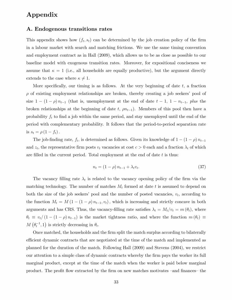
Appendix

A. Endogenous transitions rates

This appendix shows how (ft, st) can be determined by the job creation policy of the firm

in a labour market with search and matching frictions. We use the same timing convention

and employment contract as in Hall (2009), which allows us to be as close as possible to our

baseline model with exogenous transition rates. Moreover, for expositional conciseness we

assume that κ = 1 (i.e., all households are equally productive), but the argument directly

extends to the case where κ 6= 1.

More specifically, our timing is as follows. At the very beginning of date t, a fraction

ρ of existing employment relationships are broken, thereby creating a job seekers’pool of

size 1 − (1− ρ)nt−1 (that is, unemployment at the end of date t − 1, 1 − nt−1, plus the

broken relationships at the beginning of date t, ρnt−1). Members of this pool then have a

probability ft to find a job within the same period, and stay unemployed until the end of the

period with complementary probability. It follows that the period-to-period separation rate

is st = ρ (1− ft) .The job-finding rate, ft, is determined as follows. Given its knowledge of 1− (1− ρ)nt−1

and zt, the representative firm posts vt vacancies at cost c > 0 each and a fraction λt of which

are filled in the current period. Total employment at the end of date t is thus:

nt = (1− ρ)nt−1 + λtvt. (37)

The vacancy filling rate λt is related to the vacancy opening policy of the firm via the

matching technology. The number of matches Mt formed at date t is assumed to depend on

both the size of the job seekers’pool and the number of posted vacancies, vt, according to

the function Mt = M (1− (1− ρ)nt−1, vt) , which is increasing and strictly concave in both

arguments and has CRS. Thus, the vacancy-filling rate satisfies λt = Mt/vt = m (θt), where

θt ≡ vt/ (1− (1− ρ)nt−1) is the market tightness ratio, and where the function m (θt) ≡M(θ−1t , 1

)is strictly decreasing in θt.

Once matched, the households and the firm split the match surplus according to bilaterally

effi cient dynamic contracts that are negotiated at the time of the match and implemented as

planned for the duration of the match. Following Hall (2009) and Stevens (2004), we restrict

our attention to a simple class of dynamic contracts whereby the firm pays the worker its full

marginal product, except at the time of the match when the worker is paid below marginal

product. The profit flow extracted by the firm on new matches motivates —and finances—the

33

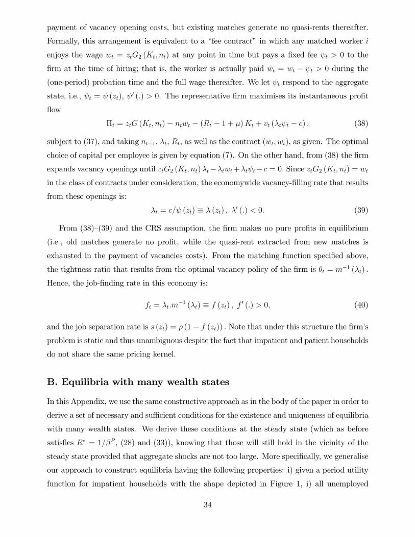
payment of vacancy opening costs, but existing matches generate no quasi-rents thereafter.

Formally, this arrangement is equivalent to a “fee contract” in which any matched worker i

enjoys the wage wt = ztG2 (Kt, nt) at any point in time but pays a fixed fee ψt > 0 to the

firm at the time of hiring; that is, the worker is actually paid wt = wt − ψt > 0 during the

(one-period) probation time and the full wage thereafter. We let ψt respond to the aggregate

state, i.e., ψt = ψ (zt), ψ′ (.) > 0. The representative firm maximises its instantaneous profit

flow

Πt = ztG (Kt, nt)− ntwt − (Rt − 1 + µ)Kt + vt (λtψt − c) , (38)

subject to (37), and taking nt−1, λt, Rt, as well as the contract (wt, wt), as given. The optimal

choice of capital per employee is given by equation (7). On the other hand, from (38) the firm

expands vacancy openings until ztG2 (Kt, nt)λt−λtwt+λtψt−c = 0. Since ztG2 (Kt, nt) = wt

in the class of contracts under consideration, the economywide vacancy-filling rate that results

from these openings is:

λt = c/ψ (zt) ≡ λ (zt) , λ′ (.) < 0. (39)

From (38)—(39) and the CRS assumption, the firm makes no pure profits in equilibrium

(i.e., old matches generate no profit, while the quasi-rent extracted from new matches is

exhausted in the payment of vacancies costs). From the matching function specified above,

the tightness ratio that results from the optimal vacancy policy of the firm is θt = m−1 (λt) .

Hence, the job-finding rate in this economy is:

ft = λt.m−1 (λt) ≡ f (zt) , f

′ (.) > 0, (40)

and the job separation rate is s (zt) = ρ (1− f (zt)) . Note that under this structure the firm’s

problem is static and thus unambiguous despite the fact that impatient and patient households

do not share the same pricing kernel.

B. Equilibria with many wealth states

In this Appendix, we use the same constructive approach as in the body of the paper in order to

derive a set of necessary and suffi cient conditions for the existence and uniqueness of equilibria

with many wealth states. We derive these conditions at the steady state (which as before

satisfies R∗ = 1/βP , (28) and (33)), knowing that those will still hold in the vicinity of the

steady state provided that aggregate shocks are not too large. More specifically, we generalise

our approach to construct equilibria having the following properties: i) given a period utility

function for impatient households with the shape depicted in Figure 1, i) all unemployed

34

household consume less than c∗; ii) all employed households consume more than c∗; iii) none

of the employed face a binding borrowing constraint; and iv) unemployed households do face

a binding borrowing constraint after m < ∞ consecutive periods of unemployment (that is,

asset liquidation takes place gradually rather than in one period, but is achieved in finite

time). For expositional clarity we focus on the case where µ = 0 (i.e., the unemployed cannot

borrow), but the argument can straightforwardly generated to the case where µ > 0.

Let us call ‘k-unemployed households’those who are unemployed for exactly k ≥ 1 con-

secutive periods at date t (and thus who were still employed at date t − k). For example,

1-unemployed households are unemployed at date t and but were employed at date t−1. Sim-

ilarly, we denote by ‘k-employed households’those employed at date t who where unemployed

from date t − k − 1 to date t − 1. By extension, 0-employed households are those employed

date t who were also employed at date t− 1.

Conjecture that i) all k-unemployed households consume the same amount cuk and hold

the same asset wealth, denoted ak; ii) all employment households hold the same asset wealth,

denoted a0; and iii) all k-employed households consume the same amount cek. We will show

that it is indeed the case in equilibrium. By assumption, the period utility function has the

following property:

u (c) =

u (c) if c ≤ c∗

u (c∗) + η (c− c∗) if c > c∗(41)

Moreover we assume that u is differentiable and strictly concave, with u′ (c) > η for all c < c∗

and limc→0+ u′ (c) = +∞. Finally, we assume that:

η < βIR∗[(1− s∗) η + s∗u′

(δI)]

(42)

We will first characterize the equilibrium wealth distribution when (42) holds. Then we

will show that when it does not, then all impatient households face a binding borrowing limit

and hence simply behave like ‘rule-of-thumb’consumers.

Consumption and asset levels. Under our conjectured equilibrium, the Euler equations

determining the distribution of wealth are:

η = βI [(1− s∗) η + s∗u′ (cu1)]R∗, (43)

u′ (cuk) = βI[f ∗η + (1− f ∗) u′

(cuk+1

)]R∗ if m ≥ 2 and for k = 1...m− 1, (44)

where (43) is the Euler equation for employed households and (44) are the Euler equations for

unemployed households before the borrowing constraint starts binding. From the households’

35

budget constraints, the consumption levels of unemployed households are

cuk = δI + ak−1R∗ − ak if m ≥ 2 and for k = 1...m− 1, (45)

cum = δI + am−1R∗, (46)

cuk = δI for k > m, (47)

while those of employed households are

cej = w∗ (1− τ ∗) + ajR∗ − a0 for j = 0, ...m (48)

The conditions for the existence of an equilibrium with m+ 1 wealth states can be stated

as follows:

cek > c∗ > cuj for all k ≥ 0 and j ≥ 1, (49)

ak > 0 for k ≥ 0, (50)

u′ (cum) > β [f ∗η + (1− f ∗) u′ (δ)]R∗. (51)

Inequality (49) ensures that the ranking of consumption levels is consistent with the as-

sumed instant utility function. Inequality (50) states that asset holdings are positive before

the constraint binds. Equation (51) states that the borrowing constraint is binding after m

periods of unemployment. We now derive a set of necessary and suffi cient conditions for

equations (43)—(51) to hold, thereby implying the existence of an equilibrium with limited

cross-sectional heterogeneity. Moreover, we will show that when this equilibrium exist, then

it is unique.

Existence and uniqueness of the equilibrium. To establish existence and uniqueness,

we first construct a function F (m, am−1) that depends on the number of liquidation periods

for unemployed households before the constraint binds (m) and the last strictly positive

wealth level before the constraint binds (am−1). If the borrowing constraints binds after m

consecutive periods of unemployment, then we know that am = 0. In words, for every possible

m, F is defined over all possible values of am−1. The goal is to use F to show that both m

and am−1 are unique given the deep parameters of the model. To construct F , note that from

(44) and (45) we have

u′(cum−1

)= βI

[f ∗η + (1− f ∗) u′

(δI + am−1R

∗)]R∗.

36

Using (44) m− 2 times to eliminate cum−1, cum−2 and c

u2 , and then (43) to eliminate c

u1 , we

obtain:

[βIR∗ (1− s∗)− 1

]η + s∗f ∗η

(βIR∗

)2

(m−2∑k=0

(βIR∗ (1− f ∗)

)k)(52)

+(βIR∗

) (βIR∗ (1− f ∗)

)m−1s∗u′

(δI + aum−1R

∗) = 0

The previous equality is valid for m ≥ 2. If m = 1, one can directly use (43) to find a0,

which corresponds to the baseline case analysed in the body of the paper.

Lemma 1 Define the function F : N×]− δ/R∗; +∞[→ R, such that

F (1, x) ≡ βIR∗s∗u′(δI + xR∗

)−[1− βIR∗ (1− s∗)

]η

and, for m ≥ 2,

F (m,x) ≡s∗f ∗η

(βIR∗

)2

1− βIR∗ (1− f ∗) −[1− βIR∗ (1− s∗)

]η (53)

+ s∗βIR∗[u′ (δ + xR∗)− f ∗ηβIR∗

1− βIR∗ (1− f ∗)

] (βIR∗ (1− f ∗)

)m−1.

Then, for any m ≥ 1, am−1 satisfies F (m, am−1) = 0.

The function F is obtained by factorising the left hand side of (52), and it only depends

on the deep parameters of the model. The following lemma uncovers some useful properties

of F .

Lemma 2 If (42) holds then

i) F is strictly decreasing in both argument

ii) For all m ≥ 1, there exists a unique xm−1 such that F (m,xm−1) = 0. Moreover, the series

xm−1 is strictly decreasing in m and we have x0 > 0 and limm→∞ xm−1 = −δI/R∗.

Proof. i) We first note that u′(δI + xR∗

)− βIR∗f∗η

(1−βIR∗(1−f∗))> 0, since 1 > βIR∗ and u′ (.) ≥ η.

Using this inequality, the expression for F (1, x) above and equation (53) withm = 2, we have

F (1, x) > F (2, x) .Moreover, for allm ≥ 2 and x > −δI/R∗ we have F (m− 1, x) > F (m,x),

that is, F (m,x) is strictly decreasing in m. Finally, F (m,x) is decreasing in x for all m

because u′ < 0. ii) Note first that limx→−δI/R∗ F (m,x) = +∞ for all m ≥ 1. Moreover,

(42) implies that F (1, 0) = βIR∗s∗u′(δI)−[1− βIR∗ (1− s∗)

]η < 0. Since F (1, x) is

continuous and monotonic in x, by the theorem of continuous functions there is an x0 such

that F (1, x0) = 0. Now, since F (m,x0) is decreasing in m we have F (2, x0) < 0; and, since

37

F (2, x) is continuous and monotonic in x, there exists a unique x1 such that F (2, x1) = 0.

Then, by induction it is easy to show that F (m,xm−2) < 0, and that, for all m ≥ 1, there

exists a unique xm−1 such that F (m,xm−1) = 0. Since F (m,x) is strictly decreasing in both

argument, the series xm−1 defined by F (m,xm−1) = 0 is decreasing in m. Finally, using (53),

one finds that F (m,xm−1) = 0 is equivalent to

u′(δI + xm−1R

∗) =1

s∗βR∗

([1− βR∗ (1− s∗)] η − s∗f ∗η (βR∗)2

1− βR∗ (1− f ∗)

)1

(βR∗ (1− f ∗))m−1

+f ∗ηβR∗

1− βR∗ (1− f ∗) (54)

The right hand side of this equation goes to +∞ as m goes to +∞. Since limc→0+ u′ (c) =

+∞, this implies that xm−1 → −δI/R∗ as m→ +∞.

Using the properties of F , we may prove the uniqueness of the equilibrium, provided that

the latter exists.

Proposition 2. If there exists an equilibrium with limited heterogeneity, then it is unique.

Moreover, borrowing constraints bind after a finite number of consecutive periods of unem-

ployment.

Proof. Define

m∗ = maxm|xm−1 ≥ 0, (55)

that is, m∗ is the largest m for which xm−1 is nonnegative. Since xm−1 is strictly decreasing,

x0 > 0 and limm→+∞ xm−1 = −δI/R∗, m∗ is finite and uniquely defined. We now show (bycontradiction) that if there exists an equilibrium with limited heterogeneity, then the borrow-

ing constraint must be binding after exactlym consecutive periods of unemployment. Suppose

that there is also an equilibrium in which households face binding borrowing constraints after

n 6= m∗ consecutive periods of unemployment. Then n would satisfy F (n, an−1) = 0. First, it

is impossible that n > m∗, since in this case we would have an−1 < 0, a contradiction. Second,

if we could find n < m∗ then we would have F (m∗, am∗−1) = F (n, an−1) (= 0). Rearranging

this equality, it can be shown that it would imply that if the borrowing constraint binds after

n consecutive periods of unemployment then am−1 < 0, a contradiction again. Thus, the only

possible equilibrium is such that m = m∗, where m∗ is finite.

We now characterize the equilibrium allocation with m∗ liquidation periods.

Lemma 3 In an equilibrium with limited heterogeneity, i) cuk is strictly decreasing in k =

1...m∗; and ii) aj is strictly decreasing in j = 0...m∗ − 1

38

Proof. i) is proven by induction. From (44), if u′ (cuk) > ηf/(1/βIR∗ − 1 + f

), then

u′(cuk+1

)> u′ (cuk) and hence c

uk+1 < cuk. Now, from (43) we have

u′ (cu1) =

(1 +

1/ (βR∗)− 1

s∗

)η.

Since βIR∗ < 1, we know that u′ (c1) > η; and since f/(1/βIR∗ − 1 + f

)< 1, it implies that

u′ (c1) > ηf/(1/βIR∗ − 1 + f

). ii) For m∗ = 1, then from (42) we have a0 > 0. For m∗ = 2,

since cum∗−1 = δI+am∗−2R∗−am∗−1 > cum = δI+am∗−1R

∗ we have am∗−2 > am∗−1 (1 + 1/R∗) >

am∗−1. For m ≥ 3, we again reason by induction. First, am∗−2 > am∗−1, for the same reason

as when m∗ = 2. Second, if am∗−2 > am∗−1 then am∗−3 > am∗−2; Indeed, from (45)-(47) and

the fact that cuk−1 > cuk, k = 0, ...m∗ − 1 we have am∗−3 − am∗−2 > (am∗−2 − am∗−1) /R∗.

We may then construct the states of the wealth distribution as follows. Given m∗ in (55),

the sequence am∗−im∗

i=0 is given by am∗ = 0, am∗−1 that solves F (m∗, am∗−1) = 0, and then

the recursion

u′(δI +R∗ak−2 − ak−1

)(56)

= βI[f ∗η + (1− f ∗) u′

(δI +R∗ak−1 − ak

)]R∗ if m∗ ≥ 2 and for 2 ≤ k ≤ m∗

until a0. This recursion also allows us to find a0 as a function of the deep parameters of the

model. Indeed, define the function G and net dis-saving Xk as follows:

G (X) = u′−1(βIR∗

[f ∗η + (1− f ∗) u′

(δI +X

)])− δI , (57)

Xk ≡ R∗ak−1 − ak. (58)

Then, (56) can be written as Xk−1 = G (Xk) for k = 2..m∗. Iterating this equation gives:

Xk = G(m∗−k) (R∗am∗−1) for k = 1...m∗ − 1,

where G(i) is the i-th iteration of G. The aks are then recovered from (58). In particular,

a0 =m∗−1∑j=1

G(j) (R∗am∗−1)

(R∗)j+

am∗−1

(R∗)m∗−1 , a1 =

m∗−2∑j=1

G(j) (R∗am∗−1)

(R∗)j+

am∗−1

(R∗)m∗−2 (59)

We can now prove the following proposition.

Proposition 3. If w∗ (1− τ ∗) − a0 > c∗ > δ + R∗a0 − a1, where a0 and a1 are given (59).

Then, the equilibrium with reduced heterogeneity exists and is unique.

Proof. We have shown that if (42) holds, then there is a unique m∗ and a unique sequence

cuk, k = 1...m such that the Euler equations (43)—(44) hold and the borrowing constraint is

39

binding afterm continuous periods of unemployment. For this allocation to be an equilibrium

with limited heterogeneity, one has to show that the ranking of consumption levels (49) is

satisfied. Since both cuk and ak are decreasing in k, cej in (48) is decreasing in j. Hence, a

suffi cient condition for the postulated ranking of consumption levels to hold is cem > c∗ > cu1 ,

which is equivalent to w∗ (1− τ ∗)− a0 > c∗ > δ +R∗a0 − a1. If this last condition hold, then

the allocation cuk , akk is the unique equilibrium.

Construction of the period utility function. Taking a utility function u and a coeffi cient

η, we can now state the conditions under which one can construct an equilibrium with limited

cross-sectional heterogeneity.

Proposition 4. For a given function u, differentiable, increasing and strictly concave and

with limc→0+ u′ (c) = +∞ and a given η > 0, one can construct an increasing and concave

utility function u such that a limited heterogeneity equilibrium exists provided that

i) w∗ (1− τ ∗)− a0 > δ +R∗a0 − a1,

ii) u′ (δ +R∗a0 − a1) ≥ η,

where a0 and a1 are given by (59).

Indeed, if i) holds, then one can finds a c∗ such that w∗ (1− τ ∗)−a0 > c∗ > δ+R∗a0−a1.

One may then construct a utility function u differentiable all over [0,∞) by smooth-pasting

u (.) with the linear part of u (.) in an arbitrarily small neighborhood of c∗. The function u

can be (weakly) concave provided that ii) holds.

C. Data

In Section 4, we use quarterly time series for real GDP and consumption, as well labour

market transition rates and total factor productivity over the period 1948Q1-2011Q1.

Real GDP is from the NIPA tables, while the real aggregate consumption series is obtained

by dividing nominal spending on nondurable goods and services by the PCE price index (all

from the NIPA tables). To compute the relevant statistics (row “data”in Table 2), the cycle

component of both series are extracted by HP-filtering the log of the series (with smoothing

parameter 1600).

For the labour-market transition probabilities, we proceed as follows. First, we compute

monthly job-finding probabilities using CPS data on unemployment and short-run unemploy-

ment, using the two-state approach of Shimer (2005, 2012). (As suggested by Shimer, 2012,

40

the short-run unemployment series is made homogenous over the entire sample by multiplying

the raw series by 1.1 from 1994M1 onwards). We then compute monthly separation prob-

abilities as residuals from a monthly flow equation similar to (1). Using these two series,

we construct transition matrices across employment statuses for every month in the sample,

and then multiply those matrices over the three consecutive months of each quarter to ob-

tain quarterly transition probabilities (this naturally implies that cyclical fluctuations in the

quarter-to-quarter separation rate partly reflect changes in the underlying monthly job-finding

rate probability).

Finally, our series for total factor productivity is computed as in Ríos-Rull and Santaeulàlia-

Llopis (2010). When estimating the joint behaviour of TFP and labour market transition

probabilities, all three series are HP-filtered with penalty parameter 1600.

References

[1] Acemoglu, D. and Autor, D.H. (2011), ‘Skills, tasks and technologies: Implications for

employment and earnings’, in O. Ashenfelter and D. Card (eds.), Handbook of Labor

Economics, Vol. 4B, Elsevier B.V., pp. 1043-1171.

[2] Aiyagari, S. R. (1994), ‘Uninsured idiosyncratic risk and aggregate saving’, Quarterly

Journal of Economics, 109, pp. 659-684.

[3] Algan, Y., Allais, O., den Haan, W.J. and Rendhal, P. (2010), ‘Solving and simulating

models with heterogeneous agents and aggregate uncertainty’, Working Paper

[4] Becker, R.A. (1980), ‘On the long-run steady state in a simple dynamic model of equilib-

rium with heterogenous households’, Quarterly Journal of Economics, 95, pp. 375-382.

[5] Becker, R.A. and Foias, C. (1987), ‘A characterization of Ramsey equilibrium’, Journal

of Economic Theory, vol. 41, pp. 173-184.

[6] Ben-Porath, Y. (1967): ‘The production of human capital and the life cycle of earnings’,

Journal of Political Economy, 75(4), pp. 352-365.

[7] Campbell, J.Y. and Mankiw, N.G. (1989), ‘Consumption, income and interest rates:

reinterpreting the time series evidence’, NBER Macroeconomics Annuals, 11, pp. 155-

201.

41

[8] Carroll, C.D. (1994), ‘How does future income affect current consumption?’, Quarterly

Journal of Economics, 109(1), pp. 111-147.

[9] Carroll, C.D. and Toche, P. (2011), ‘A tractable model of buffer stock saving’, Working

Paper.

[10] Chetty, R. (2008), ‘Moral hazard versus liquidity and optimal unemployment insurance’,

Journal of Political Economy, 116(2), pp. 173-234.

[11] Cochrane, J. (1991), ‘A simple test of consumption insurance’, Journal of Political Econ-

omy, 99, pp. 957-976

[12] Constantinides, G. and Duffi e, D. (1996), ‘Asset pricing with heterogenous consumers’,

Journal of Political Economy, 104(2), 219-240.

[13] Engen, E.M. and Gruber, J. (2001), ‘Unemployment insurance and precautionary saving’,

Journal of Monetary Economics, 47(3), pp. 545-579.

[14] Gali, J., Lopez-Salido, J.D. and Vallés, J. (2007), ‘Understanding the effects of govern-

ment spending on consumption’, Journal of the European Economic Association, 5(1),

pp. 227-270.

[15] Guerrieri, V. and Lorenzoni, G. (2011), ‘Credit crises, precautionary savings, and the

liquidity trap’, NBER Working Papers 17583.

[16] Guerrieri, V. and Lorenzoni, G. (2009), ‘Liquidity and trading dynamics’, Econometrica,

77(6), pp. 1751-1790.

[17] Gruber, J. (1997), ‘The consumption smoothing benefit of unemployment insurance’,

American Economic Review, 87, pp.192-205.

[18] Gruber, J. (1998), ‘Unemployment insurance, consumption smoothing, and private in-

surance: Evidence from the PSID and CEX’, in Research in Employment Policy, vol. 1,

L.J. Bassi and S.A. Woodbury (eds), Jai Press, Stamford, CT.

[19] Hall, R.E. (2009), ‘Reconciling cyclical movements in the marginal value of time and the

marginal product of labor’, Journal of Political Economy, 117(2), pp. 281-321.

[20] Heathcote, J. (2005), ‘Fiscal policy with heterogeneous agents and incomplete markets’,

Review of Economic Studies, 72, 161-188.

42

[21] Heathcote, J., Perri, F. and Violante, G. (2010), ‘Unequal we stand: An empirical analy-

sis of economic inequality in the United States 1967-2006’, Review of Economic Dynam-

ics, 13(1), pp. 15-51.

[22] Heathcote, J., Storesletten, K. and Violante, G.L. (2010), ‘Quantitative macroeconomics

with heterogeneous households’, Annual Review of Economics, 1, pp. 319-354.

[23] Heathcote, J., Storesletten, K. and Violante, G.L. (2009), ‘Consumption and labour

supply with partial insurance: An analytical approach’, Working Paper.

[24] Huggett, M. (1993), ‘The risk-free rate in heterogeneous-agent incomplete-insurance

economies’, Journal of Economic Dynamics and Control, 17, pp. 953-969.

[25] Iacoviello, M. (2005), ‘House prices, borrowing constraints, and monetary policy in the

business cycle’, American Economic Review, 95(3), pp. 739-764.

[26] Kaplan, G. and Violante, G.L. (2012), ‘A model of the consumption response to fiscal

stimulus payments’, Working Paper.

[27] Kiyotaki, N. and Moore, J. (1997), ‘Credit cycles’, Journal of Political Economy, 105(2),

pp. 211-248.

[28] Krusell, P., Mukoyama, T and Sahin, A. (2011), ‘Labor-market matching with precau-

tionary savings and aggregate fluctuations’, Review of Economic Studies, 77 (4), pp.

1477-1507.

[29] Krusell, P. and Smith, A.A. (1998), ‘Income and wealth heterogeneity in the macroecon-

omy’, Journal of Political Economy, 106(5), pp. 867-896.

[30] Lagos, R. and Wright, R. (2005), ‘A unified framework for monetary theory and policy

analysis’, Journal of Political Economy, 113, 463-484.

[31] Low, H., Meghir, C. and Pistaferri, L. (2010), ‘Wage risk and employment risk over the

life cycle’, American Economic Review, 100, pp. 1432—1467.

[32] McKay, A. and Reis, R. (2012), ‘The role of automatic stabilizers in the U.S. business

cycle’, Working Paper.

[33] Mankiw, N.G. (2000), ‘The savers-spenders theory of fiscal policy’, American Economic

Review, 90(2), pp. 120-125.

43

[34] Mengus, E. and Pancrazi, R. (2012), ‘Participation costs and consumption smoothing:

Theory and empirical evidence’, Working Paper.

[35] Mertens, K. and Ravn, M. (2011), ‘Understanding the aggregate effects of anticipated

and unanticipated tax policy shocks’, Review of Economic Dynamics, 14(1), pp. 27-54.

[36] Merz, M. (1995), ‘Search in the labor market and the real business cycle’, Journal of

Monetary Economics, vol. 36(2), pp. 269—300.

[37] Parker, J.A. and Preston, B. (2005), ‘Precautionary saving and consumption fluctua-

tions’, American Economic Review, 95(4), pp. 1119-1143.

[38] Ravn, M. and Sterk, V. (2012), ‘Job uncertainty and deep recessions’, Working Paper.

[39] Ríos Rull, J.-V. and Santaeulàlia-Llopis, R. (2010), ‘Redistributive shocks and produc-

tivity shocks’, Journal of Monetary Economics, 57, pp. 931-948.

[40] Rogerson, R. and Shimer, R. (2011), ‘Search in macroeconomic models of the labor

market’, in O. Ashenfelter and D. Card (eds), Handbook of Labor Economics, Vol. 4A,

Elsevier B.V., pp. 619-700.

[41] Shimer, R. (2012), ‘Reassessing the ins and outs of unemployment’, Review of Economic

Dynamics, 15(2), pp. 127-148

[42] Shimer, R. (2005), ‘The cyclical behaviour of equilibrium employment and vacancies’,

American Economic Review, 95(1), pp. 25—49.

[43] Sullivan, J.X. (2008), ‘Borrowing during unemployment: Unsecured debt as a safety net’,

Journal of Human Resources, 43, pp. 383-412.

[44] Toche (2005), ‘A tractable model of precautionary saving in continuous time,’Economics

Letters, 87(2), 267—272.

[45] Wolff, E.N. (2010), ‘Recent trends in households wealth in the US: rising debt and the

middle-class squeeze - An update to 2007’, The Levy Economic Institute Working Paper

no 589.

44