How Do Industries and Firms Respond to Changes inLocal Labor Supply?

Christian Dustmann and Albrecht Glitz

August 2012

Abstract This paper analyzes how changes in the skill mix of local labor supply are

absorbed by the economy, distinguishing between three different adjustment mechanisms:

factor prices, an expansion in the size of those production units that use the more abun-

dant skill group more intensively, and more intensive use of the more abundant skill group

within production units. We contribute to the existing literature by analyzing these ad-

justments on the firm rather than industry level and by assessing the role of new firms

in the absorption process. Drawing on unique German administrative data covering all

firms and workers over a 10 year period, we show that, although factor price adjustments

are important in the non-tradable sector, labor supply shocks do not induce factor price

changes in the tradable sector. In the latter, most adjustments to changes in relative fac-

tor supplies occur within firms through changes in relative factor intensities, which, given

the non-response of factor prices, points to changes in production technology. We further

show that firms entering and exiting the market are an important additional channel of

adjustment and that an industry level analysis is likely to overemphasize technology-based

adjustments.

Keywords: Immigration, Endogenous Technological Change, Firm Structure

JEL Codes: F1, J2, J61, L2, O3

Contact details: Albrecht Glitz, Department of Economics and Business, Universitat Pompeu Fabraand Barcelona GSE, Ramon Trias Fargas 25-27, 08005 Barcelona, Spain, email: albrecht.glitz@upf.edu;Christian Dustmann, Department of Economics, University College London, Drayton House, 30 GordonStreet, London WC1H 0AX, UK, email: c.dustmann@ucl.ac.uk. We thank Paul Beaudry, David Green,Ethan Lewis, Francesc Ortega, Ian Preston, Jan Stuhler, and seminar participants at UPF and theOutsourcing and Migration Conference in Turin for comments. We are grateful to Johannes Ludsteckand Marco Hafner from the Institute for Employment Research for invaluable support with the data. Wealso thank the Barcelona GSE Research Network, the Government of Catalonia, the Spanish Ministry ofScience (Project No. ECO2008-06395-C05-01 and ECO2011-30323-C03-02), and the Norface Programmeon Migration for their support.

1

1 Introduction

Labor economists typically assume that local economies primarily absorb changes in local

labor supply through changes in wages, and a large and growing body of literature focuses

on the magnitude of these changes.1 Open economy models, in contrast, emphasize ad-

justments to labor supply shocks through changes in the output mix, with faster growth

in firms whose use of the more abundant factor is more intensive (see Rybczynski, 1955).

More recently, shifts towards production technologies that are more intensive in the use of

the more abundant factor, either due to profit-maximizing innovators’ endogenous choice

of research direction (see e.g. Acemoglu, 1998, 2002) or firms’ selection of an optimal

production technology from a given pool of alternatives (see e.g. Beaudry and Green,

2003, 2005, and Caselli and Coleman, 2006), have been put forward as a third potential

adjustment mechanism. Existing studies that evaluate the relative magnitude of the lat-

ter two channels identify technology adjustments as the more important of the two (see

e.g. Hanson and Slaughter, 2002, Lewis, 2003, Gandal et al., 2004, Card and Lewis, 2007,

and Gonzalez and Ortega, 2011).2 These studies argue that open economy adjustments

should induce more growth in industries that make more intensive use of the relatively

more abundant type of labor, whereas technology adjustments should lead to within-

industry changes in the relative employment of the more abundant labor type. However,

analysis in these studies is performed on the industry level. Thus, if firms within an

industry produce heterogeneous products, then size adjustments between firms operating

in the same industry may be incorrectly attributed to technology-induced factor intensity

adjustments. The trade literature provides extensive evidence of product heterogeneity

even within narrowly defined industries or product categories (see, e.g., Schott, 2004, or

Broda and Weinstein, 2006), which points to a possible aggregation error.

The contribution of this paper is threefold. First, we build on and extend the existing

1See, for instance, Card (2001), Borjas (2003), Dustmann et al. (2012), Ottaviano and Peri (2012),Manacorda et al. (2012), or Glitz (2012).

2These conclusions are supported by research evidence that focuses more directly on the endogenousadoption of technology, showing that automation machinery indeed expands more rapidly in those areasin which the relative supply of skilled labor grows fastest (Lewis, 2011), and that skill abundance leadsto a faster adoption of new technologies (Beaudry et al., 2010).

2

literature by using firm-level data to quantify the channels through which immigration-

induced local labor supply shocks are absorbed into the economy, and we demonstrate

the potential aggregation error when analysis is carried out on the industry level. This is

possible by using administrative data covering all firms and workers in Germany over a

10 year period.

Second, we isolate and quantify the role of new firms entering the production process

and of dying firms leaving it in absorbing labor supply shocks. Given the high turnover of

firms, and new firms’ lower adjustment costs, not accounting for this mechanism could be

an important omission.3 Unlike other studies that are based on survey information and

cover only larger firms, our administrative data encompass the entire universe of firms,

including small firms. This is particularly important if some of the adjustments to local

labor supply shocks do indeed take place through the (net) creation of new firms, as it is

likely that small firms play a particularly important part in this process.4

Third, we assess the effect of local labor supply shocks on relative wages but differ

from existing work by distinguishing between the impact in the tradable (manufacturing)

sector and the non-tradable sector.

To perform our analysis, we draw on a unique administrative data source that covers

the entire German workforce from 1985 to 1995. The data provide not only basic worker

characteristics, including educational level, but also identifiers for the employing firms and

information on their industry affiliation. We can thus compute the skill mix employed

in each firm by aggregating workers based on the firm identifiers.5 Regional identifiers

further allow us to identify local labor markets. In addition, because the 1985-1995

period was characterized by large immigration-induced labor supply shocks, we can use

the shock component that is explainable by past immigrant settlement patterns to isolate

3In our sample and over the period we analyze, firm turnover is about 41%, a figure in line with findingsfor the United States. For example, Dunne et al. (1989a,b) find that 40% of firms in manufacturing inthe U.S. disappear over a 5-year period and are replaced by new entrants.

4For instance, Bernard and Jensen (1997) compare between and within shifts in employment on theindustry level with those calculated from a sample of manufacturing plants. However, using data fromthe U.S. Annual Survey of Manufactures (ASM), their firm sample is restricted to large manufacturingfirm that survived throughout their sampling periods (1973-1979 and 1979-1987).

5Rather than referring to firms in the legally defined sense, our data refer to business establishmentsor plants, which we believe is the appropriate unit for the purposes of our analysis. For simplicity, werefer to these as “firms”.

3

the absorption mechanisms that respond to exogenous supply shocks.6

As a first step in our analysis, we develop a simple model that illustrates the three

adjustment channels. We then provide a novel decomposition of local labor supply shocks

on the individual firm level and demonstrate that, if firms within an industry produce

heterogeneous products, an industry-level analysis may lead to overestimation of the ad-

justments related to technology-induced skill mix changes. Our decomposition method

accounts explicitly for the creation of new firms and the deaths of existing firms and we

suggest a way to decompose these firms’ contributions to overall absorption into output

and technology adjustments.

As illustrated by our simple model, the magnitude of adjustments through changes in

output mix or production technologies are difficult to interpret without considering factor

prices as an alternative channel of adjustment. In the empirical part of the analysis, we

therefore first show that, over the period that we study, immigration leads to a decrease

in the relative wages of workers in the non-tradable sector in those skill groups that

experience a relative labor supply shock, but does not change the relative wages of workers

in the tradable and manufacturing sector. This suggests that in these sectors, adjustments

have taken place through either changes in output mix or changes in technology.

The results from our main decomposition on the firm level support previous work on

the industry level (e.g. Lewis, 2003) in showing that within-firm changes in factor intensity

are more important in accommodating changes in local factor endowments, compared to

changes in output mix. For instance, in our instrumental variable regressions, the former

explains around 51% of the overall adjustment to immigration-induced labor supply shocks

in the manufacturing sector, while the latter explains only 15%. However, our findings

also show that an industry level analysis is likely to overestimate the effect commonly

assigned to technology adjustments: when the level of aggregation is reduced stepwise

from 2-digit industries to 3-digit industries and then to the firm level, the output mix

changes become relatively more important. Finally, the role of new and exiting firms in

6As an alternative to immigration-induced shocks to local labor supply, Ciccone and Peri (2011)exploit changes in compulsory schooling legislation and child labor laws across U.S. states over the period1950-1990 to study the different mechanisms through which local industry-level production structuresadjust to changes in labor supply.

4

absorbing labor supply shocks is important, and with a contribution of between 12% and

15% similar in magnitude to the estimated contribution through output mix adjustments.

The structure of the paper is as follows. In the next section, we explain our analytical

framework. In Section 3, we describe the data and provide some descriptive evidence on

the industry and firm structure in West Germany between 1985 and 1995. In Section 4,

we present our empirical results. We first show the extent to which local relative wage

rates have responded to changes in local factor supplies, and then present the main firm-

level estimates of the relative contribution of output and technology adjustments to the

absorption of local labor supply shocks. We discuss the specific role of new and old firms

in this process, and relate the firm-level results to those that would be obtained by an

industry-level analysis. Finally, we provide some additional results on the role of firm size

and nationwide changes in industry-specific production technologies. Section 5 concludes.

2 Analytical Framework

2.1 Theoretical Motivation

Suppose there are many regions R, each with production units j (j = 1, ..., J) producing

output goods Y j with a constant returns to scale technology and using i = 1, ..., K labor

inputs. In equilibrium, the factor supply in each region is equal to factor demand so that

the (K × 1) vector of factor supplies X in a particular region can be written as7

X =J∑

j=1

CjW (W,Aj)Y j. (1)

Here CjW (W,Aj) is the (K × 1) vector of unit factor demands in production unit j and

shows the units of labor input i required to produce one unit of output Y j, Aj is a (L×1)

vector of technology coefficients affecting the factor specific unit demands, and W is a

7We abstract from capital, which is equivalent to assuming that capital supply is perfectly elastic.

5

vector of factor prices. By totally differentiating (1) and rearranging terms, we obtain:

dX =J∑

j=1

Y jCjWWdW +

J∑j=1

CjWdY

j +J∑

j=1

Y jCjWAjdA

j, (2)

where CjWW is the (K×K) matrix of cross-price effects on factor demands for production

unit j, which, given our assumptions about the production technology, is negative semi-

definite; and CjWAj is a (K×L) matrix that measures the changes in unit factor demands

induced by changes in the production technology.

Considering the first term on the right-hand side of Equation (2), which reflects the

adjustment to changes in labor supply through changes in factor prices, since CjWW is

negative semi-definite, changes in factor supply and changes in wages will negatively

covary. That is, wages will decrease for workers who have the same skills as newly supplied

workers, as they become relatively more abundant but may increase for workers with other

skills.8 It should therefore be possible to detect whether local economies adjust to labor

supply shocks through factor price changes by relating changes in relative wages to changes

in relative factor supplies.

The second term on the right-hand side is the change in the output of the produc-

tion unit, weighted by the production unit-specific vector of unit factor demands. An

alternative way to absorb a supply shock, therefore, is to expand the output of those

production units that use the more abundant factor more intensively, keeping relative

unit factor demands constant. It is this adjustment channel that is postulated by open

economy models, in which output prices are set on international markets, thereby fixing

factor prices so that dW j = 0 for all j. Adjustments to factor supply shocks following this

mechanism would thus be reflected in stronger growth in production units that employ

the more abundant factor more intensively.

Finally, the last term reflects shifts in factor demands through changes in technology

8It should be noted that although relative wages and the wages of workers in the particular skill groupswill respond to changes in skill supplies, if labor is the only input into production and factor prices arethe only adjustment mechanisms, average wages will remain unchanged. Average wages will only changeif there is an additional inelastically supplied factor of production (such as capital), with the magnitudeof change depending on the elasticity of capital supply and the elasticity of substitution between capitaland skill types (see Dustmann et al., 2012, for a detailed analysis).

6

within production units when the relative size of output across production units is held

constant. In the type of model employed by Beaudry et al. (2010), this outcome could be

achieved by firms choosing different production technologies in response to labor supply

shocks, for instance, by reducing automation technology if exposed to a low skilled labor

supply shock. Hence, as in the case of adjustments through changes in the output mix

across firms, technology adjustments can contribute to the absorption of labor supply

shocks without involving changes in factor prices. Note that constant factor prices imply

that CjWAjdA

j = dCjW (W,Aj), so that the only way unit factor demands change is through

changes in technology.

2.2 Empirical Decomposition

Our empirical analysis is motivated by Equation (2). We first show that relative factor

prices in the tradable sector do not change in response to labor supply shifts, which

indicates that the first term in Equation (2) is effectively zero. We can then write the

percentage change in local labor supply in any particular skill group i relative to a base

period (denoted by subscript 0) as

∆Xi

Xi0

=J∑

j=1

CjwiY

j

Xi0

dY j

Y j+

J∑j=1

CjwiY

j

Xi0

dCjwi

Cjwi

.

Following the existing literature, we approximate Cjwi, the unit factor demand of skill

group i in production unit j, by the ratio of the number of employees of skill group i in

that production unit, Nij, to the total number of employees, Mj, so thatdCj

wi

Cjwi

= %∆(Nij

Mj).

Further, as is common in the literature, we approximate percentage changes in output Y j

by percentage changes in the total workforce Mj.9 Denoting the fraction of employment

in skill group i in production unit j relative to overall labor supply in skill group i in the

9This approximation is not unreasonable in this context and possibly a more direct measure than out-put itself given that employment is comparable across firms and our intention to capture the employmentchange embodied in output changes.

7

base period as sij0 =Nij0

Xi0, we obtain

∆Xi

Xi0

≈J∑

j=1

sij0%∆Mj +∑j

sij0%∆(Nij

Mj

). (3)

As Equation (3) shows, we capture local economies’ adjustments to factor supply shocks

through changes in the output mix and changes in production technologies within pro-

duction units using changes in production unit size (“scale effects” or “between effects”,

first term on the right) and changes in the relative use of a particular production factor

(“intensity effects” or “within effects”, second term).

In our empirical analysis, and for reasons that become clear in Section 4.1, we focus

only on the contribution of the tradable sector. As a robustness check and to facilitate

comparison with other studies (e.g., Lewis, 2011), we further restrict in some specifica-

tions the tradable sector to manufacturing firms only because their production of tradable

outputs is unambiguous. Accordingly, we first subtract from the actual observed change

in skill-specific local labor supply that part that is absorbed by the non-tradable sector.

When focusing on the manufacturing sector only, we also subtract the employment ab-

sorbed by those tradable sectors that are not manufacturing sectors. In addition, we need

to take account of unemployment in the empirical implementation. Specifically, because

our focus is on adjustments in the employment structure across and within production

units, we subtract the part of the observed change in labor supply that is absorbed through

unemployed individuals. The change in skill-specific employment in the tradable sector

is then given by ∆Ni = ∆Xi−∆NNTi −∆Ui, where ∆Ni is the change in employment of

skill group i over our observation period, and ∆Xi, ∆NNTi , and ∆Ui are the changes in

overall labor supply, employment in the non-tradable sector, and unemployment of skill

group i, respectively. Dividing the left-hand side by the total employment of skill group

i in the tradable sector in the base period, the change in skill-specific employment in all

8

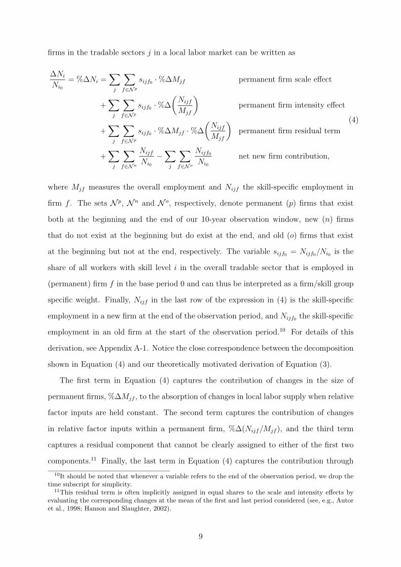
firms in the tradable sectors j in a local labor market can be written as

∆Ni

Ni0

= %∆Ni =∑j

∑f∈N p

sijf0 ·%∆Mjf permanent firm scale effect

+∑j

∑f∈N p

sijf0 ·%∆

(Nijf

Mjf

)permanent firm intensity effect

+∑j

∑f∈N p

sijf0 ·%∆Mjf ·%∆

(Nijf

Mjf

)permanent firm residual term

+∑j

∑f∈Nn

Nijf

Ni0

−∑j

∑f∈N o

Nijf0

Ni0

net new firm contribution,

(4)

where Mjf measures the overall employment and Nijf the skill-specific employment in

firm f . The sets N p, N n and N o, respectively, denote permanent (p) firms that exist

both at the beginning and the end of our 10-year observation window, new (n) firms

that do not exist at the beginning but do exist at the end, and old (o) firms that exist

at the beginning but not at the end, respectively. The variable sijf0 = Nijf0/Ni0 is the

share of all workers with skill level i in the overall tradable sector that is employed in

(permanent) firm f in the base period 0 and can thus be interpreted as a firm/skill group

specific weight. Finally, Nijf in the last row of the expression in (4) is the skill-specific

employment in a new firm at the end of the observation period, and Nijf0 the skill-specific

employment in an old firm at the start of the observation period.10 For details of this

derivation, see Appendix A-1. Notice the close correspondence between the decomposition

shown in Equation (4) and our theoretically motivated derivation of Equation (3).

The first term in Equation (4) captures the contribution of changes in the size of

permanent firms, %∆Mjf , to the absorption of changes in local labor supply when relative

factor inputs are held constant. The second term captures the contribution of changes

in relative factor inputs within a permanent firm, %∆(Nijf/Mjf ), and the third term

captures a residual component that cannot be clearly assigned to either of the first two

components.11 Finally, the last term in Equation (4) captures the contribution through

10It should be noted that whenever a variable refers to the end of the observation period, we drop thetime subscript for simplicity.

11This residual term is often implicitly assigned in equal shares to the scale and intensity effects byevaluating the corresponding changes at the mean of the first and last period considered (see, e.g., Autoret al., 1998; Hanson and Slaughter, 2002).

9

the creation and destruction of firms.

To assess how this firm-level decomposition corresponds to the industry-level decom-

position common in the empirical literature, we simply aggregate firms to a higher 2-

or 3-digit industry level, which distinguishes 79 and 296 industries, respectively.12 For a

meaningful comparison of our firm-level estimates with those for higher aggregates, we

eliminate new and exiting firms (which on the industry level are subsumed under the

corresponding industry classification) from our sample prior to estimation by adjusting

the overall change in skill-specific regional employment accordingly.13

2.3 Estimation and Identification Strategy

To obtain summary measures of the relative contribution of adjustments in scale and

intensity to the absorption of changes in local labor supply, we regress each of the com-

ponents in Equation (4) on the percentage change in employment in a region, conditional

on a full set of region fixed effects θr and skill group fixed effects λi. These latter account

for scale effects common to all firms and skill groups in a region and exogenous changes

in the relative use of different labor types in all firms and regions, respectively. In es-

timating identities, the regression coefficients for each of the single terms must sum up

to 1 so that the coefficient estimates can be interpreted as the relative contribution of

the corresponding component to the absorption of changes in labor supply on the local

level.14 For example, for the permanent firm scale effect, the estimation equation is given

by

∑jr

∑f∈N p

r

sijf0 ·%∆Mjf = yir = θr + λi + β%∆Nir + εir,

where i denotes the skill group and r the labor market region.

In interpreting the OLS parameter estimates, we first recognize that a positive estimate

12We use the 1973 industry classification provided in the IAB data.13More precisely, we obtain ∆Ni

Ni0−(∑

j

∑f∈Nn

Nijf

Ni0−∑

j

∑f∈No

Nijf0

Ni0

)≡ %∆Nperm

i .14To see that, consider the identity y = x1+x2. Regressing x1 and x2 on a constant and y gives estimates

b1 = Cov(y, x1)/V ar(y) and b2 = Cov(y, x2)/V ar(y). Since V ar(y) = V ar(x1)+V ar(x2)+2Cov(x1, x2),

b1 + b2 = 1. It is straightforward to show that the same holds for the IV estimator.

10

for β may indicate that an increase in the labor supply of, for example, low skilled workers

increases the scale of firms in affected regions that use low skilled workers more intensively.

It may equally indicate, however, that workers move to regions in which firms that use

their particular skill type more intensively are expanding in size, which implies that results

from straightforward regressions have no causal interpretation. Nonetheless, such results

are informative because they shed light on how changes in relative local labor supplies

are associated with adjustments between and within firms.

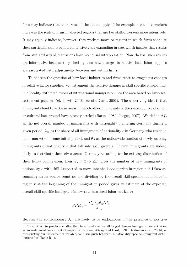
To address the question of how local industries and firms react to exogenous changes

in relative factor supplies, we instrument the relative changes in skill-specific employment

in a locality with predictions of international immigration into the area based on historical

settlement patterns (cf. Lewis, 2003; see also Card, 2001). The underlying idea is that

immigrants tend to settle in areas in which other immigrants of the same country of origin

or cultural background have already settled (Bartel, 1989, Jaeger, 2007). We define ∆Ic

as the net overall number of immigrants with nationality c entering Germany during a

given period, λcr as the share of all immigrants of nationality c in Germany who reside in

labor market r in some initial period, and θci as the nationwide fraction of newly arriving

immigrants of nationality c that fall into skill group i. If new immigrants are indeed

likely to distribute themselves across Germany according to the existing distribution of

their fellow countrymen, then λcr × θci × ∆Ic gives the number of new immigrants of

nationality c with skill i expected to move into the labor market in region r.15 Likewise,

summing across source countries and dividing by the overall skill-specific labor force in

region r at the beginning of the immigration period gives an estimate of the expected

overall skill-specific immigrant inflow rate into local labor market r:

SPRir =

∑c λcrθci∆IcXir0

.

Because the contemporary λcr are likely to be endogenous in the presence of positive

15In contrast to previous studies that have used the overall lagged foreign immigrant concentrationas an instrument for current changes (for instance, Altonji and Card, 1991; Dustmann et al., 2005), inconstructing our instrumental variable, we distinguish between 15 nationality-specific immigrant distri-butions (see Table B-1).

11

economic shocks, we use past immigrant distributions with a lag of 10 years16, which under

the plausible assumption that current regional labor market shocks are uncorrelated with

past immigrant settlement patterns leads to estimates that have a causal interpretation.

In Appendix B, we describe the composition of the immigrant population in Germany,

and the changes in composition and skill structure over the decade under study.

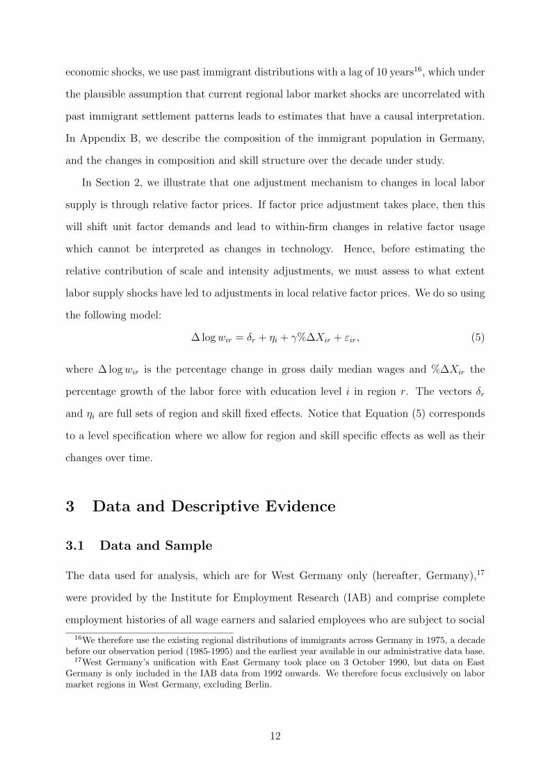
In Section 2, we illustrate that one adjustment mechanism to changes in local labor

supply is through relative factor prices. If factor price adjustment takes place, then this

will shift unit factor demands and lead to within-firm changes in relative factor usage

which cannot be interpreted as changes in technology. Hence, before estimating the

relative contribution of scale and intensity adjustments, we must assess to what extent

labor supply shocks have led to adjustments in local relative factor prices. We do so using

the following model:

∆ logwir = δr + ηi + γ%∆Xir + εir, (5)

where ∆ logwir is the percentage change in gross daily median wages and %∆Xir the

percentage growth of the labor force with education level i in region r. The vectors δr

and ηi are full sets of region and skill fixed effects. Notice that Equation (5) corresponds

to a level specification where we allow for region and skill specific effects as well as their

changes over time.

3 Data and Descriptive Evidence

3.1 Data and Sample

The data used for analysis, which are for West Germany only (hereafter, Germany),17

were provided by the Institute for Employment Research (IAB) and comprise complete

employment histories of all wage earners and salaried employees who are subject to social

16We therefore use the existing regional distributions of immigrants across Germany in 1975, a decadebefore our observation period (1985-1995) and the earliest year available in our administrative data base.

17West Germany’s unification with East Germany took place on 3 October 1990, but data on EastGermany is only included in the IAB data from 1992 onwards. We therefore focus exclusively on labormarket regions in West Germany, excluding Berlin.

12

security contributions in Germany.18 Most important for our purposes, the data also

include a unique identifier for the firm in which an individual is working in a given

year, which allows construction of a yearly panel for all firms in Germany that includes

information on the firm’s skill-specific employment and wages, industry, and region of

operation.19 The labor market regions in our analysis are aggregates of Germany’s 326

counties which take commuter flows into account in order to better reflect separate local

labor markets. Overall, there are 204 labor market regions with an average population of

around 315,000 individuals in 1995. One major advantage of using the entire workforce

is that we can observe all firms rather than being biased, as are most firm-level datasets,

toward large businesses (see, e.g., the U.S. Annual Survey of Manufactures). Since most

firms are small, with only about 20 employees the overall average firm size, such a focus

could lead to potentially misleading conclusions.

We base our analysis on all individuals aged between 15 and 64 who work full time.

We differentiate between three skill groups based on educational level, which we classify

as low, medium, and high. Individuals with a low educational level are those without

post-secondary education; those with a medium educational level have obtained post-

secondary vocational or apprenticeship degrees, and those with a high educational level

have attended college. This classification is standard in the German context (see e.g.

Antonczyk et al., 2010).

Using the 1973 industry classification provided in the IAB data, we distinguish 44

2-digit industries that produce tradable goods,20 a group in which, following Hanson

and Slaughter (2002), we include manufacturing, agriculture, mining, finance, real estate,

business services, and legal services. For a detailed overview of the individual industries

18The data do not cover the self-employed, civil servants, and the military. In 2001, 77.2% of all workersin Germany were covered by the social security system (Bundesagentur fur Arbeit, 2004).

19The wage records in the IAB data sample are top coded at the social security contribution ceiling,which can be severe for individuals in the highest skills group. Across regions, the mean fraction ofindividuals with censored wage observations is 0.6% for the low skilled, 5.0% for the medium skilled, and41.6% for the highly skilled. Hence, throughout the analysis, we use median wages and indicate wheneverthe median wage remains subject to censoring; that is, whether more than 50% of the observations withinthe highly skilled group are censored. All wages are gross daily wages in real 1995 euros based on theconsumer price index for all private households.

20Based on this industry classification, there are a further 35 industries that produce non-tradablegoods. Because the number of observations is small, we pool the following 2-digit industries: 5-8, 9-11,17/18, 23/24, 28/29, 31/32, 35/36, 47-51, 57/58, and 93/94.

13

and a number of key indicators, see Table C-1 in Appendix C. As shown in column 1 of

that table, the largest tradable industry in 1995 was manufacture of electrical equipment,

which, with around 818 thousand employees, accounted for 9.8% of the overall full-time

employment in the tradable sector in that year. Between 1985 and 1995, overall employ-

ment declined by 3.6% to around 8.2 million, but the variation in employment growth

across industries was substantial, ranging from a decrease of 51.3% in the manufacture of

apparel to an increase of 73.3% in architecture and engineering firms.

As stated above, for comparability with other studies, we limit in some specifications

the tradable sector to manufacturing industries only. In Table C-1, we use an asterisk

to designate all industries in the tradable sector that do not engage in manufacturing.21

We find that 78% of all full-time employees in the tradable sector work in manufacturing

industries. To illustrate the effect of aggregation on the estimated relative contributions

of scale and intensity adjustments, we also use a finer, 3-digit level industry classification,

which distinguishes between 296 industries.

Table 1 summarizes the most relevant information for the firms in our dataset. In

1995, a total of 402,195 firms were operating in the 44 tradable industries in the 204

labor market regions, 226,908 of them in the manufacturing sector. About half were

already in existence in 1985 (permanent firms), while another half were newly established

in the 10 years between 1985 and 1995. As could be expected, firms in the tradable

sector that existed in both 1985 and 1995 were typically larger than both new and old

firms, with 31.0 full-time employees on average in 1995, compared to 8.0 employees in new

firms and 10.1 employees in firms that were defunct by 1995. The average firm size was

23.4 full-time workers in 1985 but declined by 12.6% to 20.4 workers in 1995. Average

firm size in the manufacturing sector was somewhat larger, with 28.3 full-time workers

in 1995. In 1985, 33.5% of workers employed in the tradable sector were low skilled,

61.3% were medium skilled, and 5.2% were highly skilled.22 In the decade thereafter,

21The three biggest tradable but non-manufacturing industries are financial intermediation and insur-ance industry, legal advice and business consulting, and architecture and engineering firms.

22The share of college educated workers in the IAB data is lower than the corresponding figure fromthe microcensus because the former do not include self-employed individuals and civil servants, many ofwhom have college degrees.

14

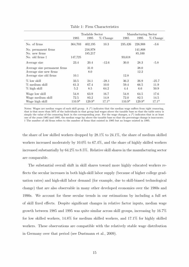
Table 1: Firm Characteristics

Tradable Sector Manufacturing Sector1985 1995 % Change 1985 1995 % Change

No. of firms 364,703 402,195 10.3 235,426 226,908 -3.6

No. permanent firms 216,978 141,808No. new firms 185,217 85,100No. old firms † 147,725 93,618

Average size 23.4 20.4 -12.6 30.0 28.3 -5.8

Average size permanent firms 31.0 38.0Average size new firms 8.0 12.2Average size old firms 10.1 12.8

% low skill 33.5 24.1 -28.1 36.2 26.9 -25.7% medium skill 61.3 67.4 10.0 59.4 66.5 11.9% high skill 5.2 8.5 64.2 4.4 6.6 50.9

Wage low skill 54.8 63.9 16.7 54.8 64.5 17.6Wage medium skill 72.5 83.2 14.8 72.0 82.5 14.5Wage high skill 110.9* 129.9* 17.1* 110.9* 129.9* 17.1*

Notes: Wages are median wages of each skill group. A (*) indicates that the median wage suffers from right censoring,that is that more than 50% of the individuals in that group had wages above the taxable base so that the table entry issimply the value of the censoring limit in the corresponding year. For the wage changes, a (*) indicates that in at leastone of the years 1985 and 1995, the median wage lay above the taxable base so that the percentage change is inaccurate.† The number of old firms refers to the number of firms that existed in 1985 but no longer existed in 1995.

the share of low skilled workers dropped by 28.1% to 24.1%, the share of medium skilled

workers increased moderately by 10.0% to 67.4%, and the share of highly skilled workers

increased substantially by 64.2% to 8.5%. Relative skill shares in the manufacturing sector

are comparable.

The substantial overall shift in skill shares toward more highly educated workers re-

flects the secular increases in both high-skill labor supply (because of higher college grad-

uation rates) and high-skill labor demand (for example, due to skill-biased technological

change) that are also observable in many other developed economies over the 1980s and

1990s. We account for these secular trends in our estimations by including a full set

of skill fixed effects. Despite significant changes in relative factor inputs, median wage

growth between 1985 and 1995 was quite similar across skill groups, increasing by 16.7%

for low skilled workers, 14.8% for medium skilled workers, and 17.1% for highly skilled

workers. These observations are compatible with the relatively stable wage distribution

in Germany over that period (see Dustmann et al., 2009).

15

3.2 Changes in Skill Mix

Figures 1 a-d illustrate the change in skill mix within regions, industries, and firms be-

tween 1985 and 1995 with a focus on medium and low skilled workers. The vertical axis

designates the log skill ratio of medium skilled workers to low skilled workers in 1995, and

the horizontal axis the corresponding ratio for 1985. Figures 1a and 1b report skill ratios

on a regional and (3-digit) industry level, while Figures 1c and 1d report skill ratios and

residuals (after region and 3-digit industry fixed effects have been removed), respectively,

on the firm level. Moving from 0 to 1, for example, corresponds to a skill ratio increase

from 1 to 2.7. We also superimpose a 45 degree (dashed) line and a regression (solid) line

regressing the 1995 skill shares on the 1985 skill shares. If the regression line is flatter

than the 45 degree line, it suggests some degree of mean reversion, with those regions

(industries, firms) that had a high skill ratio in 1985 having a smaller relative increase in

their skill ratios than regions (industries, firms) with a low skill ratio in 1985.

Figure 1a depicts not only a stark variation in skill mix across labor market regions

in both years but also a strong correlation in skill shares for both years, with regions

that had a low medium-to-low skill ratio in 1985 tending to also have a low skill ratio in

1995. The regional variation in skill ratios is quite substantial, ranging from 1.30 (1.99)

medium skilled workers for each low skilled worker at the first decile of the distribution

to 2.30 (3.68) at the ninth decile (for 1985 and 1995, respectively). The figure clearly

illustrates the large degree of skill upgrading that took place over the decade (see also

Table 1), which is best illustrated by comparing the regression line with the 45 degree

line. The figure also shows that skill shares have changed quite differentially: the change

in relative skill shares between 1985 and 1995, log(medium/low)95− log(medium/low)85,

ranges from 0.31 at the first decile to 0.60 at the ninth decile, with an average value of

0.46. Figure 1b shows similar patterns at the level of 3-digit tradable industries. Not

surprisingly, there is substantially more variation in relative skill ratios across industries

than across regions. As on the regional level, both the general skill-upgrading and the

substantial variation in relative skill ratio changes across industries are clearly visible.

Figure 1c reports the skill ratios on the firm level, conditional on these firms existing

16

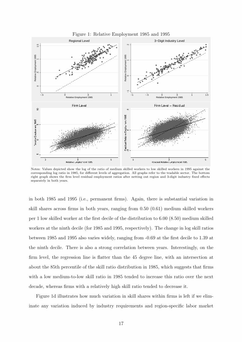
Figure 1: Relative Employment 1985 and 19950

.51

1.5

Rel

ativ

e E

mpl

oym

ent 1

995

−.5 0 .5 1Relative Employment 1985

Regional Level

−1

01

2R

elat

ive

Em

ploy

men

t 199

5

−1 −.5 0 .5 1 1.5Relative Employment 1985

3−Digit Industry Level

Notes: Values depicted show the log of the ratio of medium skilled workers to low skilled workers in 1995 against thecorresponding log ratio in 1985, for different levels of aggregation. All graphs refer to the tradable sector. The bottomright graph shows the firm level residual employment ratios after netting out region and 3-digit industry fixed effectsseparately in both years.

in both 1985 and 1995 (i.e., permanent firms). Again, there is substantial variation in

skill shares across firms in both years, ranging from 0.50 (0.61) medium skilled workers

per 1 low skilled worker at the first decile of the distribution to 6.00 (8.50) medium skilled

workers at the ninth decile (for 1985 and 1995, respectively). The change in log skill ratios

between 1985 and 1995 also varies widely, ranging from -0.69 at the first decile to 1.39 at

the ninth decile. There is also a strong correlation between years. Interestingly, on the

firm level, the regression line is flatter than the 45 degree line, with an intersection at

about the 85th percentile of the skill ratio distribution in 1985, which suggests that firms

with a low medium-to-low skill ratio in 1985 tended to increase this ratio over the next

decade, whereas firms with a relatively high skill ratio tended to decrease it.

Figure 1d illustrates how much variation in skill shares within firms is left if we elim-

inate any variation induced by industry requirements and region-specific labor market

17

conditions (and their interactions) by conditioning on a full set of 3-digit industry fixed

effects interacted with region fixed effects. Although the variation in each year decreases

considerably, from a standard deviation of 1.01 (1.05) in 1985 (1995) to a standard de-

viation of 0.85 (0.87), firms within the same 3-digit industry and the same region still

vary considerably in the skill ratios they employ. One reason could be that firms within

even quite narrowly defined industries produce heterogeneous products, which, for our

analysis, would imply that within-industry changes in skill compositions as a response to

labor supply shocks could mask between-firm scale adjustments. Within industries and

regions, the variation in the change in the relative skill mix between 1985 and 1995 ranges

from -0.98 at the first decile to 1.04 at the ninth decile.

4 Results

4.1 Wage Responses

Table 2 shows the estimates of the parameter γ in Equation (5). These estimates can be

interpreted as the percentage change in relative skill-group specific wages in response to

a 1% increase in skill group-specific labor supply. The upper panel of the table reports

results for all three education groups, while the lower panel reports results only for the low

and medium education groups. Columns 1-2 report results for non-tradable industries,

columns 3-4 give results for tradable industries, and columns 5-6 present results for the

manufacturing sector only. Uneven columns refer to OLS results and even columns to IV

results. We discuss and graphically illustrate the first-stage regressions in Appendix D.

For the non-tradable sector, our estimates indicate that changes in local labor supply

have a significantly negative impact on wages. Both OLS and IV regressions show that

relative wages decrease for those skill groups that experience supply increases. The IV

results are larger than the OLS results, which is compatible with a partial response by

regional labor supply to positive wage shocks. The results in column 2 of the upper panel,

for example, suggest that a 1% increase in the labor supply of a particular skill group

because of immigration leads to a decrease in relative median wages for workers in that

18

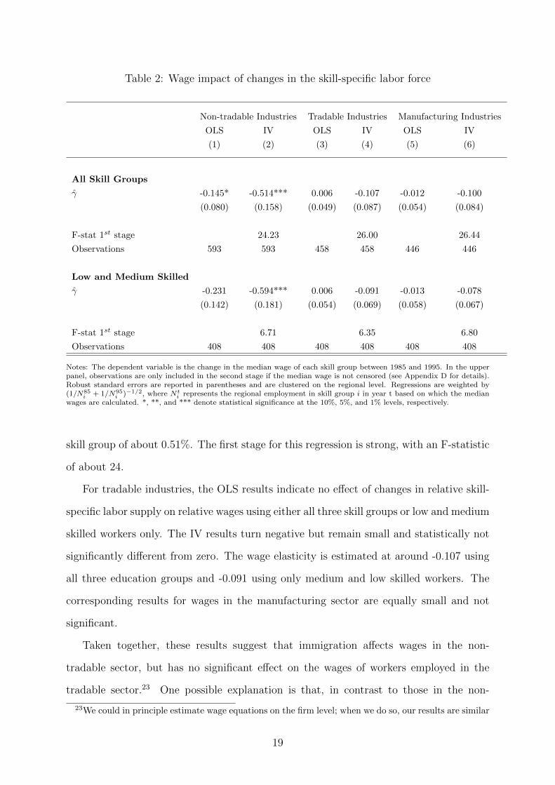
Table 2: Wage impact of changes in the skill-specific labor force

Non-tradable Industries Tradable Industries Manufacturing Industries

OLS IV OLS IV OLS IV

(1) (2) (3) (4) (5) (6)

All Skill Groups

γ -0.145* -0.514*** 0.006 -0.107 -0.012 -0.100

(0.080) (0.158) (0.049) (0.087) (0.054) (0.084)

F-stat 1st stage 24.23 26.00 26.44

Observations 593 593 458 458 446 446

Low and Medium Skilled

γ -0.231 -0.594*** 0.006 -0.091 -0.013 -0.078

(0.142) (0.181) (0.054) (0.069) (0.058) (0.067)

F-stat 1st stage 6.71 6.35 6.80

Observations 408 408 408 408 408 408

Notes: The dependent variable is the change in the median wage of each skill group between 1985 and 1995. In the upperpanel, observations are only included in the second stage if the median wage is not censored (see Appendix D for details).Robust standard errors are reported in parentheses and are clustered on the regional level. Regressions are weighted by(1/N85

i + 1/N95i )−1/2, where Nt

i represents the regional employment in skill group i in year t based on which the medianwages are calculated. *, **, and *** denote statistical significance at the 10%, 5%, and 1% levels, respectively.

skill group of about 0.51%. The first stage for this regression is strong, with an F-statistic

of about 24.

For tradable industries, the OLS results indicate no effect of changes in relative skill-

specific labor supply on relative wages using either all three skill groups or low and medium

skilled workers only. The IV results turn negative but remain small and statistically not

significantly different from zero. The wage elasticity is estimated at around -0.107 using

all three education groups and -0.091 using only medium and low skilled workers. The

corresponding results for wages in the manufacturing sector are equally small and not

significant.

Taken together, these results suggest that immigration affects wages in the non-

tradable sector, but has no significant effect on the wages of workers employed in the

tradable sector.23 One possible explanation is that, in contrast to those in the non-

23We could in principle estimate wage equations on the firm level; when we do so, our results are similar

19

tradable sector, firms in the tradable sector are unable to adjust factor prices because of

fixed output prices set on national or international markets, and that labor is insufficiently

mobile to respond to small wage changes in order to equilibrate wages across sectors.24

These findings suggest that the impact of immigration on wages should be sought in the

non-tradable rather than the tradable sector. Our study is, to the best of our knowledge,

the first that draws this distinction when estimating the wage impact of immigration.

For the subsequent analysis, the most important insight provided by Table 2 is the

absence of any large or significant effect of changes in local labor supply on wages in the

tradable sector. Within our analytical framework, this finding suggests that in that sector,

adjustments may have taken place through either changes in output mix or changes in

technology, two options we now investigate.25

4.2 Adjustments through the Output Mix, Technology, and Firm

Turnover

We now decompose the overall change in region-specific skill shares into its various com-

ponents using the decomposition presented in Equation (4), which distinguishes between

scale and intensity effects of firms that existed in both 1985 and 1995, the contribution

of new and exiting firms, and a residual term. As demonstrated in Table 1, new and

to those obtained from the regional level regressions: there is no evidence of a strong effect of changes inrelative skill-specific employment on relative wages. Results from the firm-level OLS regressions, however,by not taking into account the potential endogeneity of the changes in firm-specific relative factor inputs,fail to identify the elasticity of substitution between the different skill groups within firms. Moreover,under the reasonable assumption that labor is mobile between firms, changes in firm-specific relativefactor inputs are not expected to lead to changes in relative wages since these are determined at the labormarket rather than the firm level.

24Monras (2011) explores how such worker sluggishness could impede the adjustment process to locallabor supply shocks.

25Another reason for a differential response to labor supply shocks in tradable versus non-tradablesectors are differences in wage rigidities. It could be that wages in the tradable sector are more rigidthan in the non-tradable sector because of labor market institutions such as a wider union coverage. Toexplore this issue, we use information on the degree of union coverage in the two sectors in the year1995, provided in the IAB Establishment Panel (see Fischer et al., 2008, for details on this data set). Asexplained in Dustmann and Schonberg (2012), in Germany, all firms that are members of the employers’association pay union negotiated wages, but firms that are not members are not bound by union contractsno matter what the worker’s union status. Of the 3,921 West German firms sampled that year, 61% ofthose belonging to the non-tradable sector were covered by an industry-wide union agreement, comparedto only 51% of firms in the tradable sector. Thus, wage rigidities as a result of stronger union influenceare unlikely to explain the differential impact of labor supply shocks on wages across sectors.

20

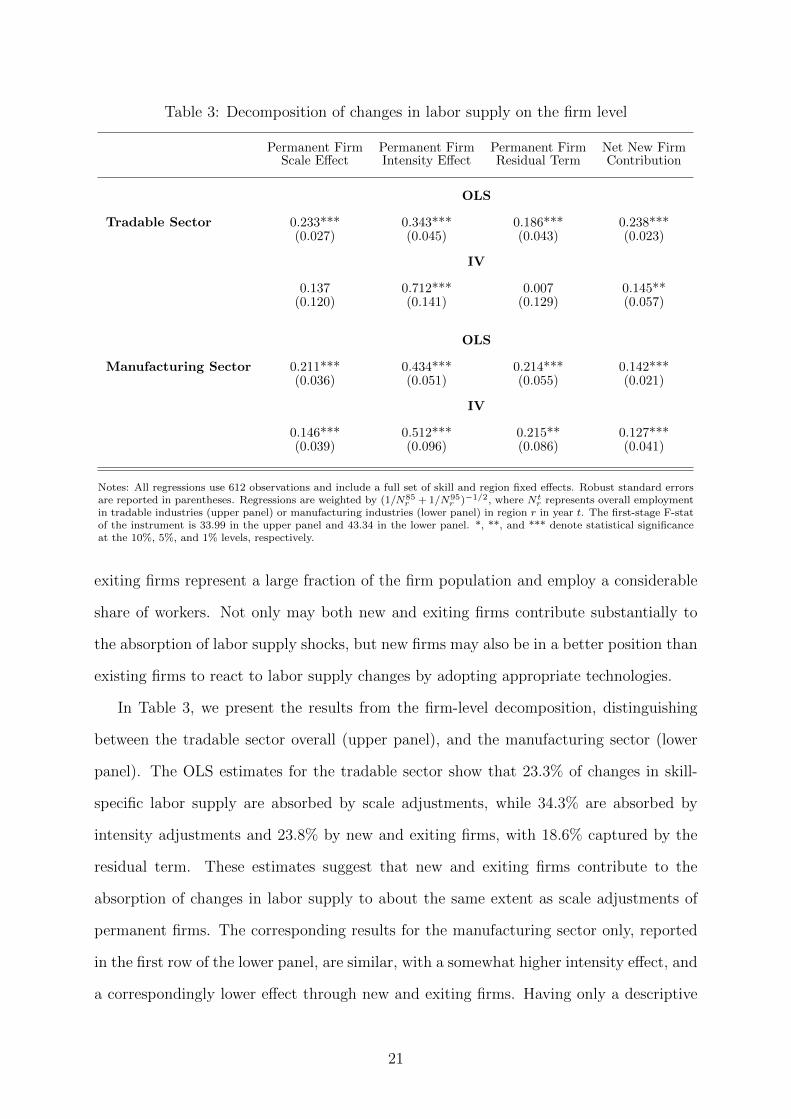
Table 3: Decomposition of changes in labor supply on the firm level

Permanent Firm Permanent Firm Permanent Firm Net New FirmScale Effect Intensity Effect Residual Term Contribution

OLS

Tradable Sector 0.233*** 0.343*** 0.186*** 0.238***(0.027) (0.045) (0.043) (0.023)

IV

0.137 0.712*** 0.007 0.145**(0.120) (0.141) (0.129) (0.057)

OLS

Manufacturing Sector 0.211*** 0.434*** 0.214*** 0.142***(0.036) (0.051) (0.055) (0.021)

IV

0.146*** 0.512*** 0.215** 0.127***(0.039) (0.096) (0.086) (0.041)

Notes: All regressions use 612 observations and include a full set of skill and region fixed effects. Robust standard errorsare reported in parentheses. Regressions are weighted by (1/N85

r + 1/N95r )−1/2, where Nt

r represents overall employmentin tradable industries (upper panel) or manufacturing industries (lower panel) in region r in year t. The first-stage F-statof the instrument is 33.99 in the upper panel and 43.34 in the lower panel. *, **, and *** denote statistical significanceat the 10%, 5%, and 1% levels, respectively.

exiting firms represent a large fraction of the firm population and employ a considerable

share of workers. Not only may both new and exiting firms contribute substantially to

the absorption of labor supply shocks, but new firms may also be in a better position than

existing firms to react to labor supply changes by adopting appropriate technologies.

In Table 3, we present the results from the firm-level decomposition, distinguishing

between the tradable sector overall (upper panel), and the manufacturing sector (lower

panel). The OLS estimates for the tradable sector show that 23.3% of changes in skill-

specific labor supply are absorbed by scale adjustments, while 34.3% are absorbed by

intensity adjustments and 23.8% by new and exiting firms, with 18.6% captured by the

residual term. These estimates suggest that new and exiting firms contribute to the

absorption of changes in labor supply to about the same extent as scale adjustments of

permanent firms. The corresponding results for the manufacturing sector only, reported

in the first row of the lower panel, are similar, with a somewhat higher intensity effect, and

a correspondingly lower effect through new and exiting firms. Having only a descriptive

21

interpretation, these OLS results, however, cannot reveal the direction of causality.

To identify firm adaptation to unforeseen labor supply shocks, we apply the IV strat-

egy explained in Section 2.3 using predictions of immigrant inflows into particular regions

and skill groups as instruments for local employment changes. For the tradable sector

as a whole, row 2 of Table 3 shows that the fraction explained by scale adjustments de-

creases to 13.7%, the contribution of within-firm adjustments increases to about 71.2%,

and the net contribution of new firms drops slightly to about 14.5%.26 Results for the

manufacturing sector are similar, although with a smaller estimate for the intensity ef-

fect. Overall, these results suggest that firm absorption of exogenously allocated workers

takes place predominantly through the employment of production technologies that use

the more abundant factor more intensively. The relatively larger scale effect estimated

in the OLS specification, in contrast, seemingly reflects scale expansions of firms attract-

ing workers into the specific labor market rather than a mechanism to absorb exogenous

changes in local labor supply. These results also show that new and exiting firms make

an important contribution to the absorption of labor supply shocks, similar in magnitude

to the absorption through changes in the output mix.27 Given its importance, and in

order to obtain an overall assessment of the relative importance of output and technology

adjustments, it would be useful to be able to interpret the new and exiting firms’ contri-

bution as either a scale or an intensity adjustment. In the next section, we propose a way

to distinguish between the two.

4.3 The Contribution of New Firms

The net new firm effect reported in Table 3 could be due to a scale effect (i.e., new firms

entering predominantly into industries that use the more abundant production factor more

intensively) or an intensity effect (i.e., new firms entering sectors that produce a particular

product choosing technologies that make more relative use of the more abundant factor).

Because these firms did not exist either at the beginning or at the end of the observation

26It should be noted that this decomposition relates only to adjustments to labor supply shifts explainedby our instruments and that in each row, the estimates must sum up to one by construction.

27It should be interesting to investigate whether immigration contributes to the start-up of new firms,as suggested in Beaudry et al. (2011). Unfortunately, we do not observe this information in our data.

22

Table 4: Decomposition of new firms’ contribution, tradable sector

Net New Firm

Scale Effect Intensity EffectEntry Over Time Entry Over Time Interaction Total

OLS

0.093*** 0.155*** -0.010 0.238***(0.028) (0.047) (0.050) (0.023)

0.028** 0.065*** 0.071*** 0.083* -0.010(0.012) (0.024) (0.018) (0.048) (0.050)

IV

0.131 0.192* -0.179 0.145**(0.115) (0.107) (0.128) (0.057)

0.055* 0.077 0.009 0.183* -0.179(0.030) (0.103) (0.029) (0.108) (0.128)

Notes: All regressions use 612 observations and include a full set of skill and region fixedeffects. Robust standard errors are reported in parentheses. Regressions are weighted by(1/N85

r + 1/N95r )−1/2, where Nt

r represents overall employment in tradable industries inregion r in year t. The first-stage F-stat of the instrument is 33.99. *, **, and *** denotestatistical significance at the 10%, 5%, and 1% levels, respectively.

window, however, we cannot use the firm-specific growth rates in scale and skill-specific

factor intensities to distinguish between the two (as in the case of permanent firms). An

alternative way to decompose the net contribution of new firms is to benchmark it against

their industry of operation in the year in which they are created or shut down. Using this

principle, for each entering or exiting firm in our 10-year observation window, we compute

the average relative factor inputs of its 2-digit industry in the year of entry or exit. The

firm’s contribution in that particular year can then be interpreted as either a pure scale

effect if its factor intensity coincides with the contemporaneous industry average, or as

an intensity effect if it enters and exits with different relative factor inputs. After the

year of entry (before the year of exit), new (old) firms can be considered permanent firms

and their growth in scale and factor intensity treated in the same way as for our initial

set of permanent firms. Following this argument, we decompose the net contribution of

new and old firms in the last row of Equation (4) into a scale component and an intensity

component, each of which is the sum of the corresponding contribution at entry or exit

and the contribution over time. For details of this decomposition, see Appendix A-2.

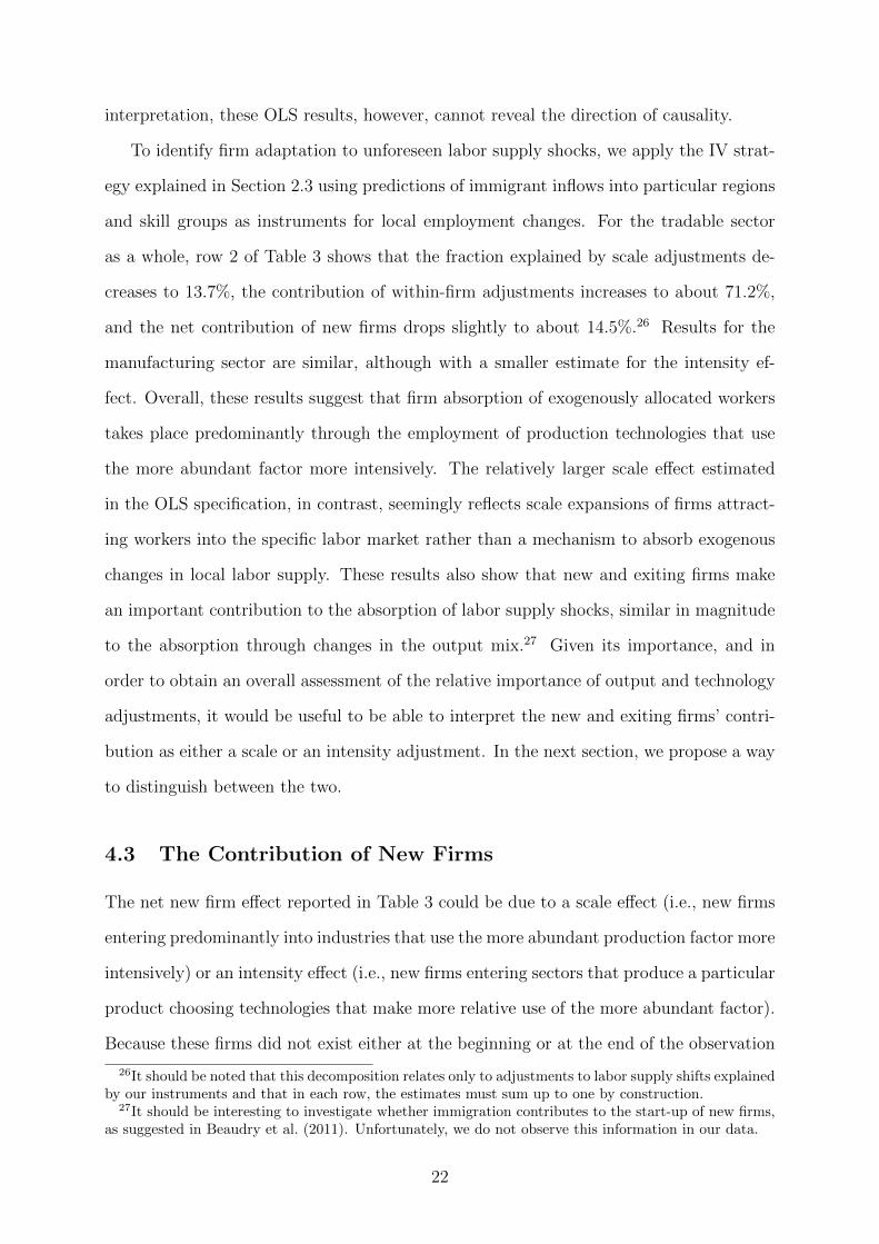
In Table 4, we report the OLS and IV results from this more detailed decomposition.

23

In the last column, we report the overall net contribution of new firms, taken directly

from Table 3. The first row of the OLS and IV panels reports the decomposition of the

net effect into an overall scale and an overall intensity effect, while the second row of each

panel reports the further decomposition into the corresponding contributions in the year

of entry/exit and over time.

Focusing on the IV results, the estimates suggest that adjustments in factor intensity,

particularly through ongoing changes after entry into the market, are the most impor-

tant channel of adjustment to exogenous changes in local labor supply. Firms entering

industries that use the more abundant factor more intensively (column 1) also appear to

contribute to the overall absorption, but to a smaller extent.

4.4 Levels of Aggregation

Like studies that use industry-level data to assess the magnitude of technology and output

mix adjustments, we also find that, even using firm-level data, technology adjustments

measured as within-firm changes in relative factor inputs are the most important channel

of adjustment to labor supply shocks. Does that mean, then, that breaking down pro-

duction units to the firm level produces essentially the same answers as an industry-level

analysis? What error would occur if we used industry-level instead of firm-level data? As

already discussed, one important shortcoming of an industry-level decomposition is the

inability to isolate the contribution of new and exiting firms to the absorption of labor

supply changes because they are subsumed under their respective industries. Moreover,

an industry-level decomposition may mask scale effects that occur across firms but within

industries, especially when firms within an industry produce heterogeneous products. To

assess the magnitude of this possible aggregation error, we decompose the adjustment

to relative labor supply changes into between and within adjustments on three levels of

aggregation: 2-digit industry, 3-digit industry, and individual firm. To make comparisons

across aggregation levels meaningful, we exclude new and exiting firms from this analysis

(see our discussion in Section 2.2).

Using only permanent firms that existed in both 1985 and 1995, we now consider the

24

correspondence between the scale effect that would be measured on the industry level

versus the firm level:28

∑j

sij0%∆Mj︸ ︷︷ ︸industry scale effect

=∑j

∑f∈N p

sijf0%∆Mjf︸ ︷︷ ︸permanent firm scale effect

+∑j

∑f∈N p

sij0

(Mjf0

Mj0

− Nijf0

Nij0

)%∆Mjf︸ ︷︷ ︸

permanent firm aggregation term scale

(6)

It follows from Equation (6) that the scale effects measured on the firm and industry level

will be the same if the last term in (6) is equal to zero, an outcome that happens trivially

if all firms in the same industry j produce with the same relative factor inputs in the

base year. In this case, (Mjf0

Mj0− Nijf0

Nij0) = 0 for all firms and the industry-based scale effect

will be identical to the firm-based scale effect. Such, however, is unlikely to be the case,

given the substantial variation in relative factor inputs across firms even within the same

industry and region (see Figure 1d). More generally, the decompositions on the industry

and firm level will lead to the same results as long as the factor intensities employed in

different firms are uncorrelated with the firms’ growth rates. If however those firms within

an industry that are particularly intensive (relative to their size) in the use of a given skill

input i (so that (Mjf0

Mj0− Nijf0

Nij0) < 0) grow at a faster rate, then the aggregation term will

be negative, meaning that an industry-level analysis will provide a lower estimate of the

contribution through scale adjustments than a firm-level analysis.

Similarly, for the intensity effect we have:

∑j

sij0%∆

(Nij

Mj

)︸ ︷︷ ︸industry intensity effect

=∑j

∑f∈Np

sijf0%∆

(Nijf

Mjf

)︸ ︷︷ ︸permanent firm intensity effect

+∑j

∑f∈Np

sijf0

( Nijf

Mjf

Nijf0

Mjf0

(Mjf

Mjf0− Mj

Mj0)

Mj

Mj0

)︸ ︷︷ ︸

permanent firm aggregation term intensity

.(7)

Equation (7) shows that the intensity effect calculated at the firm level equals the intensity

effect at the industry level if all firms in the same industry j grow at the same rate

(so if there is no “between” effect within industries); in this case, (Mjf

Mjf0− Mj

Mj0) = 0.

More generally, as long as the firms’ growth rates (relative to the industry average) are

uncorrelated with the change in their relative factor intensities, a firm-level estimation

will lead to the same results as an industry-level estimation.

28For the industry level decomposition, see Appendix A-3.

25

Table 5 reports the outcomes of distinguishing between the tradable sector (upper

panel) and manufacturing firms within the tradable sector (lower panel) for 2-digit indus-

tries, 3-digit industries, and at firm level. The first three columns report OLS results; the

last three, IV results. The OLS estimates for the tradable sector on a 2-digit industry

level suggest that 15.3% of changes in skill-specific labor supply are absorbed by scale

adjustments, while 64.4% are absorbed by intensity adjustments, with 20.3% captured by

the residual term. The relative proportion of the scale and intensity effects are almost

identical to those reported in Table 3 (about 0.68 for OLS) but are larger in absolute size

because of the focus on permanent firms only, the omission of the net new firm effects,

and the summing property of our decomposition. When we move to finer levels of dis-

aggregation (3-digit industry and firm level), the relative fraction of within adjustment

decreases, while the scale adjustment increases. This finding is compatible with the in-

tensity effect on the industry level being partially explained by scale adjustments within

industries. The figures for the manufacturing sector are similar (lower panel of the table):

again, whereas a 2-digit industry classification suggests that only 12.4% of supply changes

are absorbed by scale effects, this number increases to 17.9% when industries are broken

down into 3-digit levels and to 25.1% when the data used are on the firm level, with a

corresponding decrease in the contribution of the intensity effect. As before, however,

these OLS results allow only a descriptive interpretation.

Columns 4 to 6 of the table present the IV results. For the tradable sector as a whole,

these results show that the fraction explained by scale adjustments drops to basically zero

for the 2- and 3-digit industry classifications but increases to 16.6% when decomposed

on the firm level. As regards the manufacturing sector only, the results suggest a larger

role for scale adjustments to immigration-induced labor supply shocks. They also show,

as before, that the smaller the level of disaggregation, the larger the scale effect: on the

firm level, the numbers indicate that about 17.2% of labor supply shocks are absorbed

through scale adjustments, 56.5% through intensity adjustments, and 26.3% are captured

by the residual term.

These results suggest that aggregation may lead to an underestimation of scale ad-

26

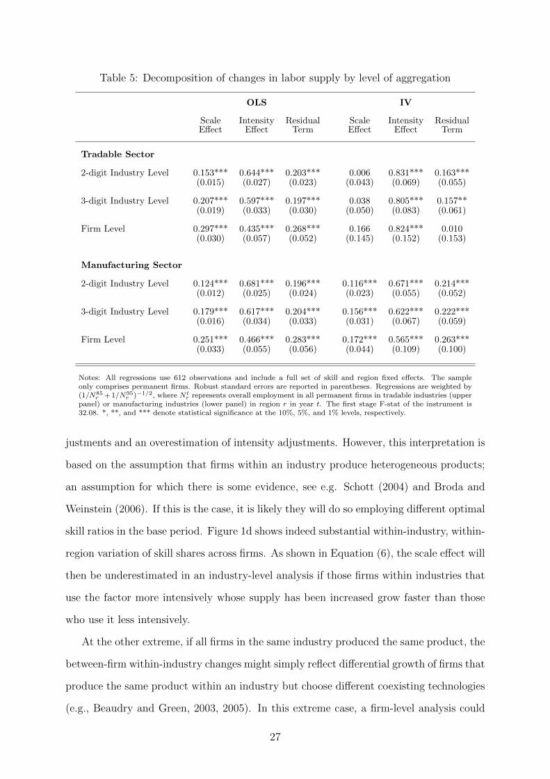
Table 5: Decomposition of changes in labor supply by level of aggregation

OLS IV

Scale Intensity Residual Scale Intensity ResidualEffect Effect Term Effect Effect Term

Tradable Sector

2-digit Industry Level 0.153*** 0.644*** 0.203*** 0.006 0.831*** 0.163***(0.015) (0.027) (0.023) (0.043) (0.069) (0.055)

3-digit Industry Level 0.207*** 0.597*** 0.197*** 0.038 0.805*** 0.157**(0.019) (0.033) (0.030) (0.050) (0.083) (0.061)

Firm Level 0.297*** 0.435*** 0.268*** 0.166 0.824*** 0.010(0.030) (0.057) (0.052) (0.145) (0.152) (0.153)

Manufacturing Sector

2-digit Industry Level 0.124*** 0.681*** 0.196*** 0.116*** 0.671*** 0.214***(0.012) (0.025) (0.024) (0.023) (0.055) (0.052)

3-digit Industry Level 0.179*** 0.617*** 0.204*** 0.156*** 0.622*** 0.222***(0.016) (0.034) (0.033) (0.031) (0.067) (0.059)

Firm Level 0.251*** 0.466*** 0.283*** 0.172*** 0.565*** 0.263***(0.033) (0.055) (0.056) (0.044) (0.109) (0.100)

Notes: All regressions use 612 observations and include a full set of skill and region fixed effects. The sampleonly comprises permanent firms. Robust standard errors are reported in parentheses. Regressions are weighted by(1/N85

r +1/N95r )−1/2, where Nt

r represents overall employment in all permanent firms in tradable industries (upperpanel) or manufacturing industries (lower panel) in region r in year t. The first stage F-stat of the instrument is32.08. *, **, and *** denote statistical significance at the 10%, 5%, and 1% levels, respectively.

justments and an overestimation of intensity adjustments. However, this interpretation is

based on the assumption that firms within an industry produce heterogeneous products;

an assumption for which there is some evidence, see e.g. Schott (2004) and Broda and

Weinstein (2006). If this is the case, it is likely they will do so employing different optimal

skill ratios in the base period. Figure 1d shows indeed substantial within-industry, within-

region variation of skill shares across firms. As shown in Equation (6), the scale effect will

then be underestimated in an industry-level analysis if those firms within industries that

use the factor more intensively whose supply has been increased grow faster than those

who use it less intensively.

At the other extreme, if all firms in the same industry produced the same product, the

between-firm within-industry changes might simply reflect differential growth of firms that

produce the same product within an industry but choose different coexisting technologies

(e.g., Beaudry and Green, 2003, 2005). In this extreme case, a firm-level analysis could

27

lead to an overestimation of the product mix adjustment and underestimation of the

technology adjustment. Thus, industry- and firm-level analyses may be interpreted as

bounds on the relative magnitude of the two different adjustment channels. In both

cases, however, according to our results, intensity adjustments are far more important for

absorbing labor supply shocks than scale adjustments, explaining between 57% and 67%

of the overall employment changes in the manufacturing sector, and between 81% and

83% in the more broadly defined tradable sector.

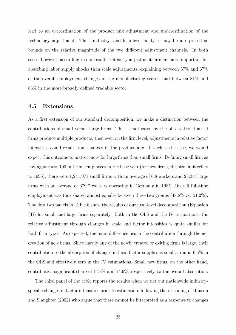
4.5 Extensions

As a first extension of our standard decomposition, we make a distinction between the

contributions of small versus large firms. This is motivated by the observation that, if

firms produce multiple products, then even on the firm level, adjustments in relative factor

intensities could result from changes in the product mix. If such is the case, we would

expect this outcome to matter more for large firms than small firms. Defining small firm as

having at most 100 full-time employees in the base year (for new firms, the size limit refers

to 1995), there were 1,241,971 small firms with an average of 6.8 workers and 23,344 large

firms with an average of 379.7 workers operating in Germany in 1985. Overall full-time

employment was thus shared almost equally between these two groups (48.8% vs. 51.2%).

The first two panels in Table 6 show the results of our firm-level decomposition (Equation

(4)) for small and large firms separately. Both in the OLS and the IV estimations, the

relative adjustment through changes in scale and factor intensities is quite similar for

both firm types. As expected, the main difference lies in the contribution through the net

creation of new firms. Since hardly any of the newly created or exiting firms is large, their

contribution to the absorption of changes in local factor supplies is small, around 6.5% in

the OLS and effectively zero in the IV estimations. Small new firms, on the other hand,

contribute a significant share of 17.3% and 14.9%, respectively, to the overall absorption.

The third panel of the table reports the results when we net out nationwide industry-

specific changes in factor intensities prior to estimation, following the reasoning of Hanson

and Slaughter (2002) who argue that these cannot be interpreted as a response to changes

28

Table 6: Decomposition of changes in labor supply on the firm level, extensions

Permanent Firm Permanent Firm Permanent Firm Net New FirmScale Effect Intensity Effect Residual Term Contribution

Large Firms OLS

0.103*** 0.171*** 0.163*** 0.065***(0.020) (0.044) (0.039) (0.020)

IV

0.006 0.388*** 0.067 -0.005(0.043) (0.138) (0.096) (0.039)

Small Firms OLS

0.130*** 0.173*** 0.023 0.173***(0.024) (0.018) (0.019) (0.016)

IV

0.131 0.325*** -0.061 0.149***(0.105) (0.046) (0.101) (0.035)

Idiosyncratic Nationwide

Nationwide OLS

0.233*** 0.276*** 0.067*** 0.186*** 0.238***(0.027) (0.045) (0.017) (0.043) (0.023)

IV

0.137 0.585*** 0.127*** 0.007 0.145**(0.120) (0.140) (0.044) (0.129) (0.057)

Notes: All regressions include a full set of skill and region fixed effects. The number of observations is 612. Robuststandard errors are reported in parentheses. Regressions are weighted by (1/N85

r + 1/N95r )−1/2, where Nt

r representsoverall employment in tradable industries in region r in year t. The first stage F-stat is 33.99. *, **, and *** denotestatistical significance at the 10%, 5%, and 1% levels, respectively.

in local labor supply. After first calculating the nationwide percentage change in factor

intensity, %∆N(Nij

Mj), for each 2-digit industry and skill group, we then subtract this change

from the actual change occurring in each permanent firm belonging to the given industry

to obtain the component of the change in relative factor intensities that is idiosyncratic

to each firm in a given region, %∆I(Nijf

Mjf):

%∆I(Nijf

Mjf

) = %∆(Nijf

Mjf

)−%∆N(Nij

Mj

).

Substituting this equality into Equation (4) leads to a new decomposition of the within-

firm effect into a component for nationwide changes in factor intensities and an idiosyn-

29

cratic region-specific component. According to the estimates in the third panel of Table

6, in Germany, the latter component plays the dominant role: in the IV estimations, 58.5

percentage points of the original 71.2% can be attributed to such idiosyncratic changes in

relative factor intensities. This finding indicates that firms in the same industries operat-

ing in different regions change their relative factor inputs differentially in response to local

changes in factor supplies: only 12.7% of the adjustment to changes in local labor supply

can be attributed to nationwide changes in industry-specific relative factor intensities.

5 Conclusion

This paper analyzes three channels by which local labor markets and the firms operating

therein can absorb skill-specific changes in labor supply: factor prices, scale adjustments

between production units, and factor intensity adjustments within production units. In

contrast to previous work, we investigate these different adjustment channels on the firm

level, which eliminates possible aggregation errors and allows an assessment of the contri-

bution of new and exiting firms. To isolate the causal effect of local supply shocks from

demand-driven supply changes, we instrument potentially endogenous changes in local

labor supply with immigrant inflows that are driven by past settlement patterns of their

co-nationals.

In a first step, we analyze the effect of changes in local labor supply on skill-specific

wages. Although we find significant wage responses in the non-tradable sector, there are

no wage effects in the tradable sector even when we instrument observed labor supply

changes. This finding suggests that it is important for studies on factor price responses

to immigration to distinguish between tradable and non-tradable sectors. Focusing on

the tradable sector (and the manufacturing sector therein), we find that more than two

thirds of the immigration-induced changes in relative skill supplies are absorbed by within-

firm changes in relative factor intensities. Given that relative factor prices are constant,

this result points to changes in production technology as an important mechanism of

adjustment to labor supply shocks.

While between-firm output mix adjustments are relatively small, the creation and

30

destruction of firms plays an important additional role in the overall adjustment to local

supply shocks. New firms enter into industries and employ relative factor intensities in

a way that is conducive to the absorption of the factor that has become relatively more

abundant.

Comparing results from an industry-level analysis with those from a firm-level analysis,

we find that the former understates the relative contribution of scale adjustments because

it does not take into account the heterogeneity of firms within an industry. In addition,

although the relative importance of the different adjustment channels on the firm level

does not vary significantly for existing firms of different sizes, the absorption through firm

turnover results predominantly from small firms entering and exiting the labor market.

Overall, our findings are in line with those reported in other studies, conducted on the

industry level, in suggesting that production technology responds endogenously to skill

mix changes. As pointed out by Lewis (2012), such endogenous responses may importantly

change the assessment of how immigration affects the labor market. Although we find

evidence for aggregation error when performing analysis on the industry level, this error

is relatively small. Our findings thus rule out that the previous industry level studies have

severely underestimated the role of output mix adjustments, and confirm the important

role of within-firm adjustments in absorbing labor supply shocks. Our analysis further

adds the insight that new and exiting firms play an important role in this adjustment

process.

31

References

Acemoglu, D. (1998). Why do new technologies complement skills? Directed technical

change and wage inequality. Quarterly Journal of Economics 113 (4), 1055–1089.

Acemoglu, D. (2002). Technical change, inequality, and the labor market. Journal of

Economic Literature 40 (1), 7–72.

Altonji, J. G. and D. Card (1991). The effects of immigration on the labor market

outcomes of less-skilled natives. In J. M. Abowd and R. B. Freeman (Eds.), Immigration,

Trade, and the Labor Market, Chapter 7, pp. 201–234. Chicago: University of Chicago

Press.

Antonczyk, D., B. Fitzenberger, and K. Sommerfeld (2010). Rising wage inequality, the

decline of collective bargaining, and the gender wage gap. Labour Economics 17 (5),

835–847.

Autor, D. H., L. F. Katz, and A. B. Krueger (1998). Computing inequality: Have com-

puters changed the labor market? Quarterly Journal of Economics 113 (4), 1169–1213.

Bartel, A. P. (1989). Where do the new U.S. immigrants live? Journal of Labor Eco-

nomics 7 (4), 371–391.

Beaudry, P., M. Doms, and E. G. Lewis (2010). Should the personal computer be con-

sidered a technological revolution? evidence from U.S. metropolitan areas. Journal of

Political Economy 118 (5), 988–1036.

Beaudry, P. and D. A. Green (2003). Wages and employment in the United States and

Germany: What explains the differences? American Economic Review 93 (3), 573–602.

Beaudry, P. and D. A. Green (2005). Changes in U.S. wages, 1976-2000: Ongoing skill

bias or major technological change? Journal of Labor Economics 23 (3), 609–648.

Beaudry, P., D. A. Green, and B. Sand (2011). How elastic is the job creation curve?

Working Paper, University of British Columbia.

32

Bernard, A. B. and J. B. Jensen (1997). Exporters, skill upgrading, and the wage gap.

Journal of International Economics 42 (1-2), 3–31.

Borjas, G. J. (2003). The labor demand curve is downward sloping: Reexamining the

impact of immigration on the labor market. Quarterly Journal of Economics 118 (4),

1335–1374.

Broda, C. and D. E. Weinstein (2006). Globalization and the gains from variety. Quarterly

Journal of Economics 121 (2), 541–585.

Bundesagentur fur Arbeit (2004). Arbeitsmarkt 2003. Amtliche Nachrichten der Bunde-

sagentur fur Arbeit.

Card, D. (2001). Immigrant inflows, native outflows, and the local labor market impacts

of higher immigration. Journal of Labor Economics 19 (1), 22–64.

Card, D. and E. G. Lewis (2007). The diffusion of Mexican immigrants during the 1990s:

Explanations and impacts. In G. J. Borjas (Ed.), Mexican Immigration to the United

States, Chapter 6, pp. 193–227. Chicago: The University of Chicago Press.

Caselli, F. and W. J. Coleman (2006). The world technology frontier. American Economic

Review 96 (3), 499–522.

Ciccone, A. and G. Peri (2011). Schooling supply and the structure of production: Evi-

dence from us states 1950-1990. NBER Working Paper 17683.

Dunne, T., M. J. Roberts, and L. Samuelson (1989a). The growth and failure of U.S.

manufacturing plants. Quarterly Journal of Economics 104 (4), 671–698.

Dunne, T., M. J. Roberts, and L. Samuelson (1989b). Plant turnover and gross em-

ployment flows in the U.S. manufacturing sector. Journal of Labor Economics 7 (1),

48–71.

Dustmann, C., F. Fabbri, and I. Preston (2005). The impact of immigration on the British

labour market. Economic Journal 115 (507), F324–F341.

33

Dustmann, C., T. Frattini, and I. Preston (2012). The effect of immigration along the

distribution of wages. Review of Economic Studies, forthcoming .

Dustmann, C., J. Ludsteck, and U. Schonberg (2009). Revisiting the german wage struc-

ture. Quarterly Journal of Economics 124 (2), 843–881.

Dustmann, C. and U. Schonberg (2012). What makes firm-based vocational training

schemes successful? The role of commitment. American Economic Journal: Applied

Economics 4 (2), 36–61.

Fischer, G., F. Janik, D. Muller, and A. Schmucker (2008). The iab establishment panel

– from sample to survey to projection. FDZ Methodenreport No. 01/2008.

Gandal, N., G. H. Hanson, and M. J. Slaughter (2004). Technology, trade, and adjustment

to immigration in Israel. European Economic Review 48 (2), 403–428.

Glitz, A. (2012). The labor market impact of immigration: A quasi-experiment exploiting

immigrant location rules in Germany. Journal of Labor Economics .

Gonzalez, L. and F. Ortega (2011). How do very open economies absorb large immigration

flows? Recent evidence from Spanish regions. Labour Economics, forthcoming 18 (1),

57–70.

Hanson, G. H. and M. J. Slaughter (2002). Labor-market adjustment in open economies:

Evidence from US states. Journal of International Economics 57 (1), 3–29.

Jaeger, D. A. (2007). Green cards and the location choices of immigrants in the United

States, 1971-2000. Research in Labor Economics 27, 131–183.

Lewis, E. G. (2003). Local open economies within the U.S.: How do industries respond

to immigration. Federal Reserve Bank of Philadelphia Working Paper No. 04-1.

Lewis, E. G. (2011). Immigration, skill mix, and capital-skill complementarity. Quarterly

Journal of Economics 126 (2), 1029–1069.

Lewis, E. G. (2012). Immigration and production technology. Mimeo, Dartmouth College.

34

Manacorda, M., A. Manning, and J. Wadsworth (2012). The impact of immigration on

the structure of wages: Theory and evidence from Britain. Journal of the European

Economic Association 10 (1), 120–151.

Monras, J. (2011). The sluggish movement of workers: Rethinking immigration absorp-

tion, Rybczynski effects and wage responses. Mimeo.

Ottaviano, G. I. P. and G. Peri (2012). Rethinking the effect of immigration on wages.

Journal of the European Economic Associationg 10 (1), 152–197.

Rybczynski, T. M. (1955). Factor endowments and relative commodity prices. Econom-

ica 22 (88), 336–341.

Schott, P. K. (2004). Acrossproduct versus withinproduct specialization in international

trade. Quarterly Journal of Economics 119 (2), 647–678.

35

Appendix A Decompositions

Appendix A-1 Firm-level Decomposition

The change in skill-specific employment in all tradable industries j in a local labor market

is given by:

∆Ni =∑j

∆Nij

=∑j

(∑

f∈Np

∆Nijf +∑

f∈Nn

∆Nijf +∑

f∈No

∆Nijf ).

Dividing by the total employment of skill group i in the base period (denoted by subscript

0) and then expanding gives

∆Ni

Ni0

=∑j

(∑

f∈Np

∆Nijf

Ni0

+∑

f∈Nn

∆Nijf

Ni0

+∑

f∈No

∆Nijf

Ni0

)

=∑j

∑f∈Np

Nijf0

Ni0

∆Nijf

Nijf0

+∑j

∑f∈Nn

∆Nijf

Ni0

+∑j

∑f∈No

Nijf0

Ni0

∆Nijf

Nijf0

=∑j

∑f∈Np

sijf0%∆Nijf +∑j

∑f∈Nn

Nijf

Ni0

−∑j

∑f∈No

Nijf0

Ni0

,

(A-1)

where sijf0 =Nijf0

Ni0.

Setting Mjf as a measure of firm size, then for all permanent firms, we can decompose

the first term of Equation (A-1) into the following three terms:

%∆Nijf =∆Nijf

Nijf0

=MjfNijf

Nijf0Mjf− Mjf0Nijf0

Nijf0Mjf0

=MjfNijf

Nijf0Mjf− 1

=NijfMjf0

MjfNijf0

+(Mjf −Mjf0)Nijf

MjfNijf0

− 1

=Mjf −Mjf0

Mjf0

+NijfMjf0

MjfNijf0

− 1 +Mjf −Mjf0

Mjf0

(NijfMjf0

MjfNijf0

− 1

)

=

(Mjf −Mjf0

Mjf0

)+

( Nijf

Mjf− Nijf0

Mjf0

Nijf0

Mjf0

)+

(Mjf −Mjf0

Mjf0

)( Nijf

Mjf− Nijf0

Mjf0

Nijf0

Mjf0

)

= %∆Mjf + %∆

(Nijf

Mjf

)+ %∆Mjf ·%∆

(Nijf

Mjf

).

Plugging this expression into Equation (A-1) yields the basic firm level decomposition

given in Equation (4).

36

Appendix A-2 New/Old Firm Decomposition

The terms involving new and old firms can be decomposed as follows:

∑j

∑f∈Nn

Nijf

Ni0

=

T∑t=1

∑j

∑f∈Nn

t

Nijft

Ni0

+

T∑t=1

∑j

∑f∈Nn

t

∆Tt Nijft

Ni0

=

T∑t=1

(∑j

∑f∈Nn

t

(Nijt

Ni0

)(Mjft

Mjt

)+∑j

∑f∈Nn

t

(Nijt

Ni0

)(Mjft

Mjt

)( Nijft

Mjft− Nijt

Mjt

Nijt

Mjt

))

+

T∑t=1

(∑j

∑f∈Nn

t

Nijft

Ni0

∆Tt Nijft

Nijft

)

=

T∑t=1

∑j

∑f∈Nn

t

(Nijt

Ni0

)(Mjft

Mjt

)︸ ︷︷ ︸

new firm entry scale

+

T∑t=1

∑j

∑f∈Nn

t

(Nijt

Ni0

)(Mjft

Mjt

)( Nijft

Mjft− Nijt

Mjt

Nijt

Mjt

)︸ ︷︷ ︸

new firm entry intensity

+

T∑t=1

∑j

∑f∈Nn

t

Nijft

Ni0

%∆Tt Mjft︸ ︷︷ ︸

new firm growth scale

+

T∑t=1

∑j

∑f∈Nn

t

Nijft

Ni0

%∆Tt

(Nijft

Mjft

)︸ ︷︷ ︸

new firm growth intensity

+

T∑t=1

∑j

∑f∈Nn

t

Nijft

Ni0

%∆Tt Mjft%∆T

t

(Nijft

Mjft

)︸ ︷︷ ︸

new firm growth residual

∑j

∑f∈No

Nijf0

Ni0

=

T−1∑t=0

∑j

∑f∈No

t

Nijft

Ni0

−T−1∑t=0

∑j

∑f∈No

t

∆t0Nijft

Ni0

=

T−1∑t=0

(∑j

∑f∈No

t

(Nijt

Ni0

)(Mjft

Mjt

)+∑j

∑f∈No

t

(Nijt

Ni0

)(Mjft

Mjt

)( Nijft

Mjft− Nijt

Mjt

Nijt

Mjt

))

−T−1∑t=0

(∑j

∑f∈No

t

Nijf0

Ni0

∆t0Nijft

Nijf0

)

=

T−1∑t=0

∑j

∑f∈No

t

(Nijt

Ni0

)(Mjft

Mjt

)︸ ︷︷ ︸

old firm exit scale

+

T−1∑t=0

∑j

∑f∈No

t

(Nijt

Ni0

)(Mjft

Mjt

)( Nijft

Mjft− Nijt

Mjt

Nijt

Mjt

)︸ ︷︷ ︸

old firm exit intensity

−T−1∑t=0

∑j

∑f∈No

t

Nijf0

Ni0

%∆t0Mjft︸ ︷︷ ︸

old firm growth scale

−T−1∑t=0

∑j

∑f∈No

t

Nijf0

Ni0

%∆t0

(Nijft

Mjft

)︸ ︷︷ ︸

old firm growth intensity

−T−1∑t=0

∑j

∑f∈No

t

Nijf0

Ni0

%∆t0Mjft%∆t

0

(Nijft

Mjft

)︸ ︷︷ ︸

old firm growth residual

37

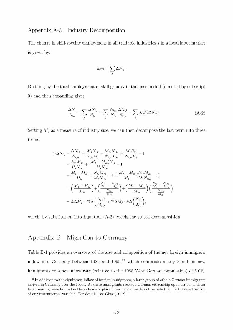
Appendix A-3 Industry Decomposition

The change in skill-specific employment in all tradable industries j in a local labor market

is given by:

∆Ni =∑j

∆Nij .

Dividing by the total employment of skill group i in the base period (denoted by subscript

0) and then expanding gives

∆Ni

Ni0

=∑j

∆Nij

Ni0

=∑j

Nij0

Ni0

∆Nij

Nij0

=∑j

sij0%∆Nij . (A-2)

Setting Mj as a measure of industry size, we can then decompose the last term into three

terms:

%∆Nij =∆Nij

Nij0

=MjNij

Nij0Mj− Mj0Nij0

Nij0Mj0

=MjNij

Nij0Mj− 1

=NijMj0

MjNij0

+(Mj −Mj0)Nij

MjNij0

− 1

=Mj −Mj0

Mj0

+NijMj0

MjNij0

− 1 +Mj −Mj0

Mj0

(NijMj0

MjNij0

− 1)

=

(Mj −Mj0

Mj0

)+

( Nij

Mj− Nij0

Mj0

Nij0

Mj0

)+

(Mj −Mj0

Mj0

)( Nij

Mj− Nij0

Mj0

Nij0

Mj0

)

= %∆Mj + %∆

(Nij

Mj

)+ %∆Mj ·%∆

(Nij

Mj

),

which, by substitution into Equation (A-2), yields the stated decomposition.

Appendix B Migration to Germany

Table B-1 provides an overview of the size and composition of the net foreign immigrant

inflow into Germany between 1985 and 1995,29 which comprises nearly 3 million new

immigrants or a net inflow rate (relative to the 1985 West German population) of 5.0%.

29In addition to the significant inflow of foreign immigrants, a large group of ethnic German immigrantsarrived in Germany over the 1990s. As these immigrants received German citizenship upon arrival and, forlegal reasons, were limited in their choice of place of residence, we do not include them in the constructionof our instrumental variable. For details, see Glitz (2012).

38

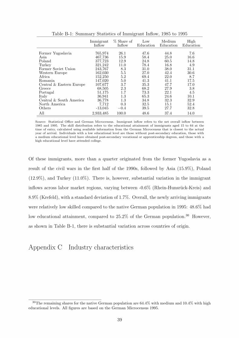
Table B-1: Summary Statistics of Immigrant Inflow, 1985 to 1995

Immigrant % Share of Low Medium HighInflow Inflow Education Education Education

Former Yugoslavia 765,974 26.1 47.6 44.8 7.6Asia 467,736 15.9 58.4 25.0 16.6Poland 377,723 12.9 24.8 60.5 14.8Turkey 321,242 11.0 78.4 16.8 4.9Former Soviet Union 243,767 8.3 31.0 38.0 31.1Western Europe 162,030 5.5 27.0 42.4 30.6Africa 152,250 5.2 69.4 22.0 8.7Romania 147,020 5.0 41.3 41.1 17.5Central & Eastern Europe 107,677 3.7 35.3 47.7 17.0Greece 68,505 2.3 68.2 27.9 3.8Portugal 51,175 1.7 73.3 22.1 4.5Italy 36,941 1.3 65.3 24.6 10.1Central & South America 36,778 1.3 34.8 32.3 32.9North America 7,712 0.3 32.5 15.1 52.4Others -13,045 −0.4 39.5 27.7 32.8

All 2,933,485 100.0 48.6 37.4 14.0

Source: Statistical Office and German Microcensus. Immigrant inflow refers to the net overall inflow between1985 and 1995. The skill distribution refers to the educational attainment of immigrants aged 15 to 64 at thetime of entry, calculated using available information from the German Microcensus that is closest to the actualyear of arrival. Individuals with a low educational level are those without post-secondary education, those witha medium educational level have obtained post-secondary vocational or apprenticeship degrees, and those with ahigh educational level have attended college.

Of these immigrants, more than a quarter originated from the former Yugoslavia as a

result of the civil wars in the first half of the 1990s, followed by Asia (15.9%), Poland

(12.9%), and Turkey (11.0%). There is, however, substantial variation in the immigrant

inflows across labor market regions, varying between -0.6% (Rhein-Hunsruck-Kreis) and

8.9% (Krefeld), with a standard deviation of 1.7%. Overall, the newly arriving immigrants

were relatively low skilled compared to the native German population in 1995: 48.6% had

low educational attainment, compared to 25.2% of the German population.30 However,

as shown in Table B-1, there is substantial variation across countries of origin.

Appendix C Industry characteristics

30The remaining shares for the native German population are 64.4% with medium and 10.4% with higheducational levels. All figures are based on the German Microcensus 1995.

39

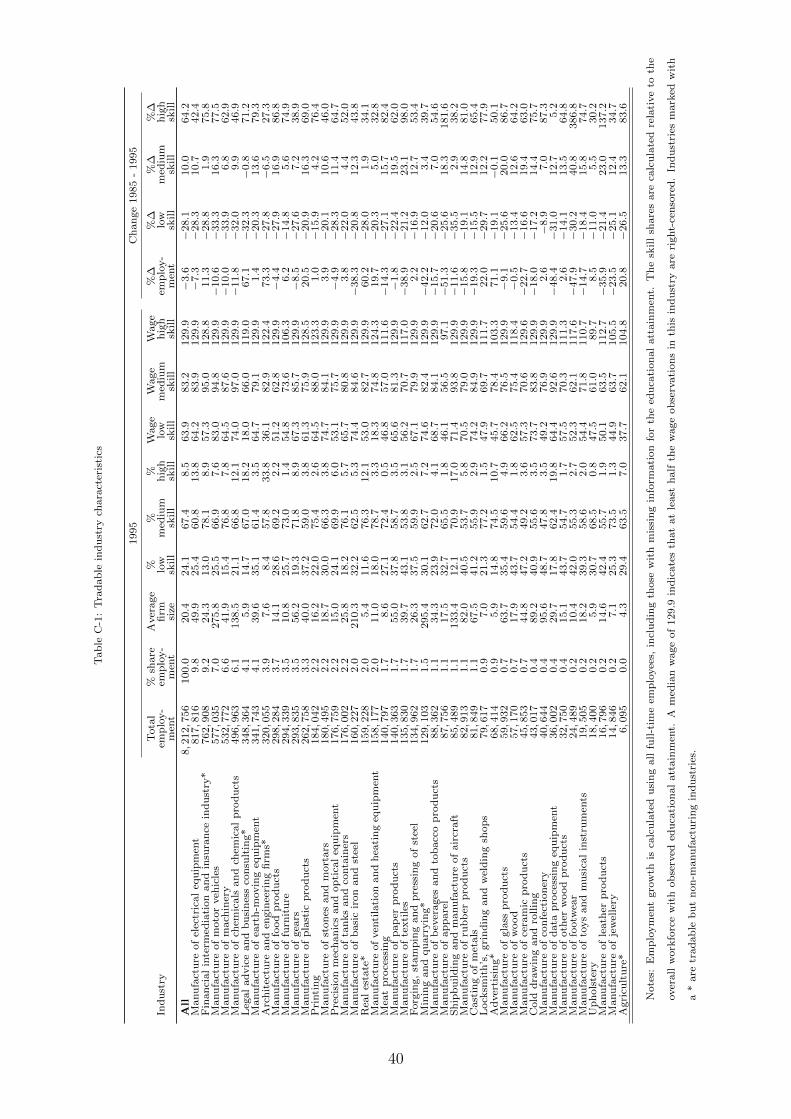
Tab

leC

-1:

Tra

dab

lein

du

stry

chara

cter

isti

cs

1995

Ch

an

ge

1985

-1995

Tota

l%

share

Aver

age

%%

%W

age

Wage

Wage

%∆

%∆

%∆

%∆

Ind

ust

ryem

plo

y-

emp

loy-

firm

low

med

ium

hig

hlo

wm

ediu

mh

igh

emp

loy-

low

med

ium

hig

hm

ent

men

tsi

zesk

ill

skil

lsk

ill

skill

skill

skill

men

tsk

ill

skill

skill

All

8,2

12,7

56

100.0

20.4

24.1

67.4

8.5

63.9

83.2

129.9

−3.6

−28.1

10.0

64.2

Manu

fact

ure

of

elec

tric

al

equ

ipm

ent

817,8

16

9.8

49.9

25.4

60.8

13.8

64.2

83.9

129.9

−7.3

−28.3

10.7

42.4

Fin

an

cial

inte

rmed

iati

on

an

din

sura

nce

ind

ust

ry*

762,9

08

9.2

24.3

13.0

78.1

8.9

57.3

95.0

128.8

11.3

−28.8

1.9

75.8

Manu

fact

ure

of

moto

rveh

icle

s577,0

35

7.0

275.8

25.5

66.9

7.6

83.0

94.8

129.9

−10.6

−33.3

16.3

77.5

Manu

fact

ure

of

mach

iner

y532,7

72

6.6

41.9

15.4

76.8

7.8

64.5

87.6

129.9

−10.0

−33.9

6.8

62.9

Manu

fact

ure

of

chem

icals

an

dch

emic

al

pro

du

cts

496,9

63

6.1

138.5

21.1

66.8

12.1

74.0

97.0

129.9

−11.8

−32.0

9.9

46.9

Leg

al

ad

vic

ean

db

usi

nes

sco

nsu

ltin

g*

348,3

64

4.1

5.9

14.7

67.0

18.2

18.0

66.0

119.0

67.1

−32.3

−0.8

71.2

Manu

fact

ure

of

eart

h-m

ovin

geq

uip

men

t341,7

43

4.1

39.6

35.1

61.4

3.5

64.7

79.1

129.9

1.4

−20.3

13.6

79.3

Arc

hit

ectu

rean

den

gin

eeri

ng

firm

s*320,0

55

3.9

7.6

8.4

57.8

33.8

36.1

82.9

122.4

73.3

−27.8

−6.5

27.3

Manu

fact

ure

of

food

pro

du

cts

298,2

84

3.7

14.1

28.6

69.2

2.2

51.2

62.8

129.9

−4.4

−27.9

16.9

86.8

Manu

fact

ure

of

furn

itu

re294,3

39

3.5

10.8

25.7

73.0

1.4

54.8

73.6

106.3

6.2

−14.8

5.6

74.9

Manu

fact

ure

of

gea

rs293,8

35

3.5

56.2

19.3

71.8

8.9

67.3

85.7

129.9

−8.5

−27.6

7.2

38.9

Manufa

ctu

reof

pla

stic

pro

du

cts

262,7

58

3.3

40.0

37.2

59.0

3.8

61.3

75.9

128.5

20.5

−20.9

16.3

69.0

Pri

nti

ng

184,0

42

2.2

16.2

22.0

75.4

2.6

64.5

88.0

123.3

1.0

−15.9

4.2

76.4

Manu

fact

ure

of

ston

esan

dm

ort

ars

180,4

95

2.2

18.7

30.0

66.3

3.8

74.7

84.1

129.9

3.9

−20.1

10.6

46.0

Pre

cisi

on

mec

han

ics

an

dop

tica

leq

uip

men

t176,7

59

2.2

15.0

24.1

69.9

6.0

53.1

75.7

129.9

−4.9

−28.3

11.4

64.7

Manu

fact

ure

of

tan

ks

an

dco

nta

iner

s176,0

02

2.2

25.8

18.2

76.1

5.7

65.7

80.8

129.9

3.8

−22.0

4.4

52.0

Manu

fact

ure

of

basi

cir

on

an

dst

eel

160,2

27

2.0

210.3

32.2

62.5

5.3

74.4

84.6

129.9

−38.3

−20.8

12.3

43.8

Rea

les

tate

*159,2

28

2.0

5.4

11.6

76.3

12.1

53.0

82.7

129.9

60.2

−28.0

1.9

34.1

Manu

fact

ure

of

ven

tila

tion

an

dh

eati

ng

equ

ipm

ent

158,1

77

2.0

11.0

18.0

78.7

3.3

18.3

74.8

124.3

19.7

−20.3

5.0

32.8

Mea

tp

roce

ssin

g140,7

97

1.7

8.6

27.1

72.4

0.5

46.8

57.0

111.6

−14.3

−27.1

15.7

82.4

Manu

fact

ure

of

pap

erp

rod

uct

s140,3

63

1.7

55.0

37.8

58.7

3.5

65.6

81.3

129.9

−1.8

−22.4

19.5

62.0

Manu

fact

ure

of

texti

les

135,8

30

1.7

39.7

43.1

53.8

3.1

56.2

70.7

117.0

−38.9

−21.2

23.1

98.0

Forg

ing,

stam

pin

gan

dp

ress

ing

of

stee

l134,9

62

1.7

26.3

37.5

59.9

2.5

67.1

79.9

129.9

2.2

−16.9

12.7

53.4

Min

ing

an

dqu

arr

yin

g*

129,1

03

1.5

295.4

30.1

62.7

7.2

74.6

82.4

129.9

−42.2

−12.0

3.4

39.7

Manu

fact

ure

of

bev

erages

an

dto

bacc

op

rod

uct

s88,3

62

1.1

34.3

23.9

72.0

4.1

68.7

84.1

129.9

−15.7

−20.6

7.0

54.6

Manu

fact

ure

of

ap

pare

l87,7

56

1.1

17.5

32.7

65.5

1.8

46.1

56.5

97.1

−51.3

−25.6

18.3

181.6

Sh

ipb

uild

ing

an

dm

anu

fact

ure

of

air

craft

85,4

89

1.1

133.4

12.1

70.9

17.0

71.4

93.8

129.9

−11.6

−35.5

2.9

38.2

Manu

fact

ure

of

rub

ber

pro

du

cts

82,9

13

1.1

82.0

40.5

53.7

5.8

70.5

79.0

129.9

−15.8

−19.1

14.8

81.0

Cast

ing

of

met

als

81,8

49

1.1

67.5

41.2

55.9

2.9

74.2

84.9

129.9

−19.3

−15.5

12.9

65.4

Lock

smit

h’s

,gri

nd

ing

an

dw

eld

ing

shop

s79,6

17

0.9

7.0

21.3

77.2

1.5

47.9

69.7

111.7

22.0

−29.7

12.2

77.9

Ad

ver

tisi

ng*

68,4

14

0.9

5.9

14.8

74.5

10.7

45.7

78.4

103.3

71.1

−19.1

−0.1

50.1

Manu

fact

ure

of

gla

ssp

rod

uct

s59,9

32

0.7

63.7

35.4

59.6

4.9

66.2

76.5

129.9

−9.1

−25.6

20.0

86.7

Manu

fact

ure

of

wood

57,1

70

0.7

17.9

43.7

54.4

1.8

62.5

75.4

118.4

−0.5

−13.4

12.6

64.2

Manu

fact

ure

of

cera

mic

pro

du

cts

45,8

53

0.7

44.8

47.2

49.2

3.6

57.3

70.6

129.6

−22.7

−16.6

19.4

63.0

Cold

dra

win

gan

dro

llin

g43,0

17

0.4

89.2

40.9

55.6

3.5

73.7

83.8

129.9

−18.0

−17.2

14.4

75.7

Manu

fact

ure

of

con

fect

ion

ery

40,6

44

0.4

95.6

48.7

47.8

3.5

49.2

76.9

129.9

2.6

−8.9

7.0

87.3

Manu

fact

ure

of

data

pro

cess

ing

equ

ipm

ent

36,0

02

0.4

29.7

17.8

62.4

19.8

64.4

92.6

129.9

−48.4

−31.0

12.7

5.2

Manu

fact

ure

of

oth

erw

ood

pro

du

cts

32,7

50

0.4

15.1

43.7

54.7

1.7

57.5

70.3

111.3

2.6

−14.1

13.5

64.8

Manu

fact

ure

of

footw

ear

24,4

89

0.2

10.4

42.0

55.3

2.7

52.3

62.1

117.6

−47.9

−30.2

40.8

386.8

Manu

fact

ure

of

toys

an

dm

usi

cal

inst

rum

ents

19,5

05

0.2

18.2

39.3

58.6

2.0

54.4

71.8

110.7

−14.7

−18.4

15.8

74.7

Up

hols

tery

18,4

00

0.2

5.9

30.7

68.5

0.8

47.5

61.0

89.7

8.5

−11.0

5.5

30.2

Manu

fact

ure

of

leath

erp

rod

uct

s16,7

96

0.2

14.6

42.4

55.7

1.9

50.1

63.5

112.7

−35.9

−21.4

23.0

137.2

Manu

fact

ure

of

jew

elle

ry14,8

46

0.2

7.1

25.3

73.5

1.3

44.9

63.7

105.5

−23.5

−25.1

12.4

34.7

Agri

cult

ure

*6,0

95

0.0

4.3

29.4

63.5

7.0

37.7

62.1

104.8

20.8

−26.5

13.3

83.6

Note

s:E

mp

loym

ent

gro

wth

isca

lcu

late

du

sin

gall

full-t

ime

emp

loyee

s,in

clu

din

gth

ose

wit

hm

issi

ng

info

rmati

on

for

the

edu

cati

on

al

att

ain

men

t.T

he

skill

share

sare

calc

ula

ted

rela

tive

toth

e

over

all

work

forc

ew

ith

ob

serv

eded

uca

tion

al

att

ain

men

t.A

med

ian

wage

of

129.9

ind

icate

sth

at

at

least

half

the

wage

ob

serv

ati

on

sin

this

ind

ust

ryare

right-

cen

sore

d.

Ind

ust

ries

mark

edw

ith

a*

are

trad

ab

leb

ut

non

-manu

fact

uri

ng

ind

ust

ries

.

40

Appendix D The First Stage

In Figures 2a-d, we show the relation between our instrument (described in Section 2.3)

and local labor supply changes, both overall and separately by skill group, by plotting

the percentage change in local labor supply against the predicted inflow of immigrants

and the corresponding (weighted) regression line, after previously netting out region and

education group fixed effects. All regressions are based on the weights for the tradable

sector. As the figures show, there is a strong positive relationship between the changes

in labor supply and the predicted immigrant inflow rates for the low and medium skill

groups, with a slope coefficient of 0.407 and 0.410, respectively, and a somewhat weaker

relationship for the high skill group, with a slope coefficient of 0.180. Overall, the first-

stage relation between our instrument and the change in local labor supply for the pooled

sample of all three skill groups (see Figure 2a) is strong, with a slope parameter of 0.297

and a standard error of 0.058, yielding a first stage F-statistic of 26.00.

Note that we use all 612 available region/skill cells in the first stage regression, but only

those observations for which the median wage is not subject to censoring in the second

stage regression. LetX, Y and Z be the regressor, outcome and instrument matrices for all

possible observations (after netting out region and skill fixed effects), and X∗, Y ∗ and Z∗

the corresponding matrices for the set of observations with uncensored median wages, then

the estimator is given by γ =(X ′Z(Z ′Z)−1(Z∗

′Z∗)(Z ′Z)−1Z ′X

)−1(X ′Z)(Z ′Z)−1Z∗

′Y ∗,

which is a consistent estimator of γ under the assumption of random censoring. Based

on this estimator, standard errors, clustered on the regional level, are obtained in the

standard way.31 Restricting both the first and the second stage regressions to the set of

observations for which the median wage is not subject to censoring does not significantly

affect the magnitude of the estimated wage effects. In this case, they amount to -0.490

(0.151) in the non-tradable sector, -0.085 (0.069) in the tradable sector, and -0.080 (0.068)

in the manufacturing sector.

31Specifically, V ar(γ) =(X ′Z(Z ′Z)−1(Z∗

′Z∗)(Z ′Z)−1Z ′X

)−1

X ′Z(Z ′Z)−1(∑

r Z∗′r uru

′rZ∗r

)(Z ′Z)−1Z ′X(

X ′Z(Z ′Z)−1(Z∗′Z∗)(Z ′Z)−1Z ′X

)−1

, where ur = Y ∗r −X∗r γ.

41

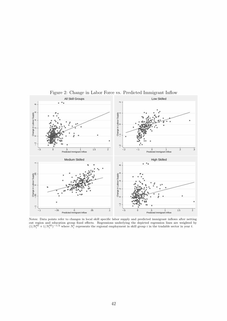
Figure 2: Change in Labor Force vs. Predicted Immigrant Inflow

−.2

0.2

.4.6

.8C

hang

e in

Lab

our

Sup

ply

−.5 0 .5 1 1.5 2Predicted Immigrant Inflow

All Skill Groups

−.2

−.1

0.1

.2C

hang

e in

Lab

our

Sup

ply

−.2 −.1 0 .1 .2 .3Predicted Immigrant Inflow

Low Skilled

−.1

−.0

50

.05

.1C

hang

e in

Lab

our

Sup

ply

−.1 −.05 0 .05 .1Predicted Immigrant Inflow

Medium Skilled

−.2

0.2

.4.6

.8C

hang

e in

Lab

our

Sup

ply

−.5 0 .5 1 1.5 2Predicted Immigrant Inflow

High Skilled

Notes: Data points refer to changes in local skill specific labor supply and predicted immigrant inflows after nettingout region and education group fixed effects. Regressions underlying the depicted regression lines are weighted by(1/N85

i + 1/N95i )−1/2 where Nt

i represents the regional employment in skill group i in the tradable sector in year t.

42