Embed Size (px)
Citation preview
How Do Location Decisions of Firms and Households Affect Economic Development in Rural America?
JunJie Wu Agricultural and Resource Economics
200A Ballard Extension Hall Oregon State University
Corvallis, OR 97331 Phone: 541-737-3060 Fax: 541-737-2563
E-mail: [email protected]
Munisamy Gopinath Agricultural and Resource Economics
212A Ballard Extension Hall Oregon State University
Corvallis, OR 97331 Phone: 541-737-1402 Fax: 541-737-2563
E-mail: [email protected]
Selected Paper prepared for presentation at the American Agricultural Economic Association
Annual Meeting, Providence, Rhode Island, July 24-27, 2005 Copyright 2005 by JunJie Wu and Munisamy Gopinath. All rights reserved. Readers may make any verbatim copies of this document for non-commercial purpose by any means, provided that this copyright notice appears on such copies.
2
How Do Location Decisions of Firms and Households Affect Economic Development in Rural America?
Abstract
This paper examines the causes of spatial inequalities in economic development across rural America. A theoretical model is developed to analyze interactions between location decisions of firms and households as they are affected by natural endowments, accumulated human and physical capital, and economic geography. Based on the theoretical analysis, an empirical model is specified to quantify the effect of these factors on key indicators of economic development across counties in the United States. Preliminary results suggest that households are willing to trade better amenities for lower income, and firms take advantage of lower wage rates by locating in areas with better climate and more recreational opportunities. In equilibrium, counties with better climate and more creational opportunities have lower income and more employment opportunities. Accumulated human and physical capital also significantly affect economic development across counties in the United States. Counties with more accumulated human and physical capital have higher income, more employment opportunities, and high development density. Remoteness has a negative effect on every measure of economic development indicator. It reduces income, employment, housing prices and total developed areas. Implications of the results for policy development to promote economic prosperity in rural America are discussed. Key words: Accumulated human and physical capital, amenities, economic development, economic geography, employment, housing price, land development, natural endowments, rural income.
How Do Location Decisions of Firms and Households Affect Economic
Development in Rural America?
For at least 30 years, dramatic social and economic changes have occurred in rural America.
Shifting population, income losses, declining education and health services, and the weakening
community structures have caused the quality of life to deteriorate in many rural communities.
Increased global competition, changes in market structure, growing population, and increasing
demands for recreational and environmental services from land and water resources have also
changed the global environment within which the farm sector operates. These dramatic changes
have created opportunities for some rural communities and raised new barriers for others.
Economic development is highly uneven between rural and urban communities as well as
within rural areas. From 1969 to 2000, average earnings per job in the United States increased
approximately 30 percent, while average earnings per job in rural America declined slightly.
The unemployment and poverty rates were 10% and 28% higher, respectively, in rural America
than in non-rural area in 2001 (Economic Research Service, 2004). These statistics have fueled
the perceived rural-urban divide. In addition, there exists a large variance in economic
development among rural communities. In some rural communities (e.g., rural Dakotas),
dwindling rural economies have caused once-viable communities to become ghost towns. In
others (e.g., rural California), urban development and suburbanization have encroached on rural
communities.
What causes the rural-urban divide? Why do the spatial inequalities in economic
development exist among rural communities? Why the spatial differences in land rents and
wages not bid away by households and firms in search of high income and low production costs?
2
What policies are effective to stimulate economic growth in distressed rural communities?
Understanding these issues is central for understanding many aspects of economic
underdevelopment in rural communities and for developing effective policies to promote vitality
and quality of life for rural Americans (Henderson et al., 2001).
Previous studies have identified three major factors as determining the spatial inequalities
in economic development: a) natural endowments (e.g., water availability, land quality,
environmental amenities); b) accumulated human and physical capital, and c) economic
geography (see the literature review in the next section). These theories, however, have rarely
been tested in the context of rural America, and little evidence exists as to what works in
improving economic conditions in rural communities and how community actions and policy
makers can strengthen the economic fabric in rural communities. Yet, understanding the relative
contribution of these factors is central for understanding many aspects of economic development
in rural communities, including the role of local and regional policies such as public
infrastructure investments in shaping the pattern of economic activities in rural America.
The objective of this article is to evaluate the contributions of natural endowments,
accumulated human and physical capital, and economic geography to the spatial inequalities in
economic development in rural America. To this end, we first develop a theoretical model to
analyze the interaction between location decisions of firms and households as they are affected
by natural endowments, accumulated capital, and economic geography. We then conduct an
empirical analysis to quantify the effect of natural endowments, accumulated capital, and
economic geography on the spatial distribution of economic development activities across
counties in the United States. Implications of the results for policy development to promote
economic prosperity in rural America are discussed.
3
This paper develops a theoretical model to analyze the interactions between the location
decisions of firms and households, which has rarely been analyzed in previous studies. It also
fills a gap in the economic literature by evaluating the relative contributions of natural
endowments, accumulated human and physical capital, and economic geography to the spatial
variability in economic development across rural America. The results of this study should be of
interest to a wide spectrum of individuals and groups. Empirical results regarding the relative
contribution of natural endowment, accumulated capital, and economic geography to economic
development should help rural counties as well as state and federal agencies develop more
effective strategies for economic development in rural America. Data and methods used to
model the interactions between firms and households and between private and public sectors
should be of great interest to researchers working in the areas of rural development. The results
of this analysis should also be of interest to conservationists and the public at-large who feel
strongly about rural issues.
Relevant Literature
Much research has focused on location decisions of households and firms in urban and regional
economics, but relatively few analyze the interaction between these locations. According to the
classic theory, a household chooses the residential location that provides the best tradeoff
between land costs and commuting costs. Wealthier households live in suburbs if and only if the
income elasticity of demand for housing is larger than the income elasticity of commuting cost.
Wheaton (1977) provides empirical evidence that questions the validity of this theory.
In searching for alternative explanations, many economists have turned to factors
excluded from the simple monocentric model, such as availability of new suburban housing, the
flight from central-city problems, transportation modes, and suburban zoning (e.g., LeRoy and
4
Sonstelie, 1983). Other economists suggest that cause and effect are simultaneous. Urban fiscal
disparities and city decay are not only the causes of middle class flight, but the product as well
(Bradford and Oates, 1974) The fragmented structure of local government and the presence of
racial and social externalities are the primary forces that originally generated middle class flight
(Tiebout, 1956). More recently, Brueckner et al. (1999) and Wu (2003) show that the location
pattern of different income groups can be explained by the distribution of amenities over the
landscape. These studies, however, do not consider the location decisions of firms and thus
sources of household income.
In the public economics literature, several studies have focused on location decisions of
households and the equilibrium structure of local jurisdictions (Epple and Romer 1991,
Fernandez and Rogerson, 1996, Epple and Sieg, 1999). Although these studies provide strong
predictions about community characteristics, they do not consider the location decisions of firms,
nor the role of amenities and geography in the formation of municipal structure. More recently,
Wu (2003) develops an equilibrium model to analyze the spatial pattern of land development and
community characteristics. He shows that the spatial distribution of amenities and commuting
costs are important factors determining the spatial patterns of land development and community
characteristics (e.g., the level of public services and the ratio of low- to high-income households).
This study, however, does not consider the interaction between the location decisions of firms
and households.
Firm location decisions have also been at the center of economic research for many
decades (Giannias and Liargovas 2002). According to Fujita et al. (1999), firms' location
decisions are based both on input price considerations and on ease of access to markets. Firms
want to locate close to input markets to save transportation costs. So a location with a lot of firms

5
will have a high demand for intermediate goods, making it an attractive location for intermediate
producers. This in turn makes it an attractive location for firms that use intermediate goods. Thus,
there is a positive feedback between location decisions of upstream and downstream firms in the
chain of economic activity (Henderson et al., 2001). Firms also want to locate close to demand
and population centers. As a disproportionate share of manufacturing is attracted to a location,
either the wage rate is bid up or labor is attracted to the location, both of which will tend to
increase this location's share of total expenditure still further. This "home market" or
agglomeration effect has been explored in Krugman (1991).
Many studies also examine the impact of taxes on firm location decisions. These studies
generally produce inconclusive and inconsistent results (see Rainey and McNamara (1999) for an
review). Rainey and McNamara (1999) examine the impact of local tax differentials on the
location of manufacturing firms and find that firms tend to avoid counties that have relatively
high property tax rates. This suggests that tax relief incentives can be an important component of
a county's industrial recruitment program.
Giannias and Liargovas (2002) view spatial variations in economic development as a
result of firm and household location decisions. They develop an economic model to examine
the behavior of households and firms and apply the model to 17 Arab countries. This study,
however, does not examine the relative contribution of natural endowment and accumulated
capital to economic development because regional differences are measured by a single index.
A number of theoretical studies have also analyzed spatial variations in economic
development across regions/countries. Henderson, et al. (2001) review these studies and suggest
that the spatial inequalities in economic development have to do partly with spatial variations in
institutions and endowments, and partly also to do with the spatial relationship between
6
economic units. However, relatively few studies have examined the effect of these factors on
economic development empirically, particularly in the context of rural development.1 Deller et
al. (2001) estimate a structure model of regional economic growth to determine the role of
amenity and quality of life attributes in regional economic growth. They find that there exist
predictable relationships between amenities, quality of life and local economic performance.
Other studies suggest that quality of life plays an increasingly important role in community
economic growth (e.g., Dissart and Deller, 2000; Halstead and Deller, 1997; Rudzitis, 1999;
Gottlieb, 1994).2 In cross-country studies, Redding and Venables (2000) examine the
relationships between geographic characteristics, wage, and per capita income. Gallup and Sachs
(1999) regress national per capita income on four variables (a measure of hydro-carbons per
capita, a dummy variable for incidence of malaria, the proportion of population who live within
100 km of the coast, international transportation costs) and find that these four variables alone
account for an astonishing 69% of the per capita income variations across their sample of 83
countries. Rappaport and Sachs (2002) analyze the effect of coastal proximity on the
concentration of economic activity in the U.S. using regression and find that the costal
concentration derives primarily from a productivity effect but also, increasingly, from a quality-
of-life effect. To our knowledge, no study has evaluated the relative contribution of natural
endowments, accumulated capital, and economic geography to spatial variations in economic
activity across counties in the United States.
Theoretical Model
1 A few studies have examined the impact of geography on land development patterns. See, e.g., Irwin and Bockstael (2002) and Wu (2001). 2 See Castle (1995) for a review and analysis of changing American countryside.
7
This section present a model to analyze the interactions between location decisions of firms and
households as they are affected by natural endowments, accumulated human and physical
capital, and economic geography. To be consistent with the empirical analysis, the model selects
county as the basic unit of analysis. County is the smallest geographic unit at which most
economic data are reported at the national level. County is also the basic political unit
(jurisdiction) in which many local regulations and policies are developed. Counties differ by
natural endowments, accumulated human and physical capital, and economic geography. Some
of these natural, institutional and geographical factors directly affect households’ utility, others
directly affect firms’ output and/or production costs. Those directly affecting households’ utility
and residential location decisions are referred to as amenities and are indexed by e , and those
directly affecting firms’ location decisions are referred to as capital and are indexed by k . Thus,
counties are differentiated by ( , )e k , and rural counties generally have higher /e k ratios than
urban counties.
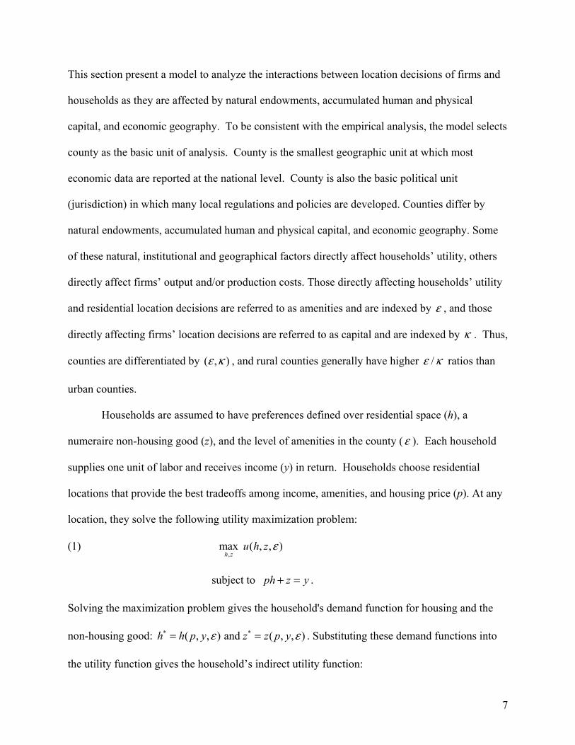
Households are assumed to have preferences defined over residential space (h), a
numeraire non-housing good (z), and the level of amenities in the county (e ). Each household
supplies one unit of labor and receives income (y) in return. Households choose residential
locations that provide the best tradeoffs among income, amenities, and housing price (p). At any
location, they solve the following utility maximization problem:
(1) ,
max ( , , )h z
u h z e
subject to ph z y+ = .
Solving the maximization problem gives the household's demand function for housing and the
non-housing good: * *( , , ) and ( , , )h h p y z z p ye e= = . Substituting these demand functions into
the utility function gives the household’s indirect utility function:
8
(2) * *( , , ) ( , , )v y p u h ze e∫
Equation (2) implies that when choosing residential locations, households consider the
tradeoffs between income, amenities and housing prices. Thus, both the total supply of the labor
( sL ) and the total demand for residential development ( dH ) in a county are functions of income
(y), amenities (e ), and housing prices (p):
(3) ( , , )s sL L y p e=
(4) ( , , )d dH H y p e=
If households are assumed to be completely mobile, and migration is costless.
Equilibrium for households requires that utility is the same in all counties, that is, ( , , ) ,v y p ve =
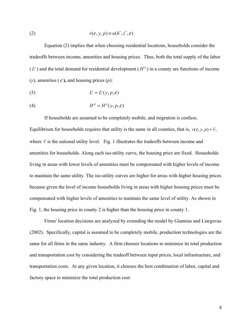
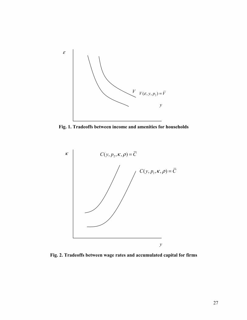
where v is the national utility level. Fig. 1 illustrates the tradeoffs between income and
amenities for households. Along each iso-utility curve, the housing price are fixed. Households
living in areas with lower levels of amenities must be compensated with higher levels of income
to maintain the same utility. The iso-utility curves are higher for areas with higher housing prices
because given the level of income households living in areas with higher housing prices must be
compensated with higher levels of amenities to maintain the same level of utility. As shown in
Fig. 1, the housing price in county 2 is higher than the housing price in county 1.
Firms' location decisions are analyzed by extending the model by Giannias and Liargovas
(2002). Specifically, capital is assumed to be completely mobile, production technologies are the
same for all firms in the same industry. A firm chooses locations to minimize its total production
and transportation cost by considering the tradeoff between input prices, local infrastructure, and
transportation costs. At any given location, it chooses the best combination of labor, capital and
factory space to minimize the total production cost:
9
(5) , ,( , , ) min
subject to ( , , , ) ,
p
L K Hc y p yl rk ps
f l k s z
k
k
∫ + +
=
where l, k, and s are labor, capital, and factory space, respectively, f (.) is the production
function, Z is the total output. The firm's transportation cost, tc , is a function of its location
characteristics r : ( )t tc c r= .
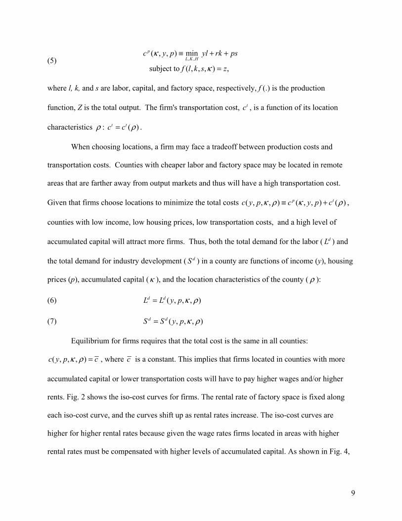
When choosing locations, a firm may face a tradeoff between production costs and
transportation costs. Counties with cheaper labor and factory space may be located in remote
areas that are farther away from output markets and thus will have a high transportation cost.
Given that firms choose locations to minimize the total costs ( , , , ) ( , , ) ( )p tc y p c y p ck r k r∫ + ,
counties with low income, low housing prices, low transportation costs, and a high level of
accumulated capital will attract more firms. Thus, both the total demand for the labor ( dL ) and
the total demand for industry development ( dS ) in a county are functions of income (y), housing
prices (p), accumulated capital (κ ), and the location characteristics of the county ( r ):
(6) ( , , , )d dL L y p k r=
(7) ( , , , )d dS S y p k r=
Equilibrium for firms requires that the total cost is the same in all counties:
( , , , )c y p ck r = , where c is a constant. This implies that firms located in counties with more
accumulated capital or lower transportation costs will have to pay higher wages and/or higher
rents. Fig. 2 shows the iso-cost curves for firms. The rental rate of factory space is fixed along
each iso-cost curve, and the curves shift up as rental rates increase. The iso-cost curves are
higher for higher rental rates because given the wage rates firms located in areas with higher
rental rates must be compensated with higher levels of accumulated capital. As shown in Fig. 4,
10
the rental rate in county 2 is higher than the one in county 1.
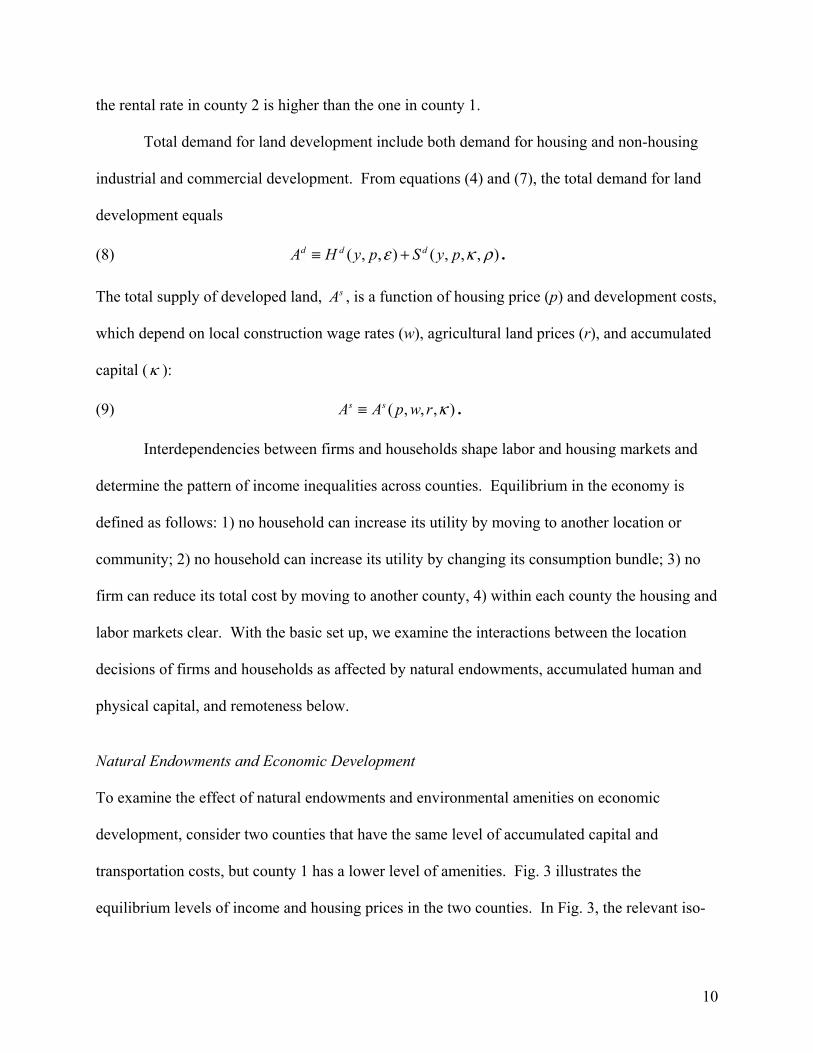
Total demand for land development include both demand for housing and non-housing
industrial and commercial development. From equations (4) and (7), the total demand for land
development equals
(8) ( , , ) ( , , , )d d dA H y p S y pe k r∫ + .
The total supply of developed land, sA , is a function of housing price (p) and development costs,
which depend on local construction wage rates (w), agricultural land prices (r), and accumulated
capital (κ ):
(9) ( , , , )s sA A p w r k∫ .
Interdependencies between firms and households shape labor and housing markets and
determine the pattern of income inequalities across counties. Equilibrium in the economy is
defined as follows: 1) no household can increase its utility by moving to another location or
community; 2) no household can increase its utility by changing its consumption bundle; 3) no
firm can reduce its total cost by moving to another county, 4) within each county the housing and
labor markets clear. With the basic set up, we examine the interactions between the location
decisions of firms and households as affected by natural endowments, accumulated human and
physical capital, and remoteness below.
Natural Endowments and Economic Development
To examine the effect of natural endowments and environmental amenities on economic
development, consider two counties that have the same level of accumulated capital and
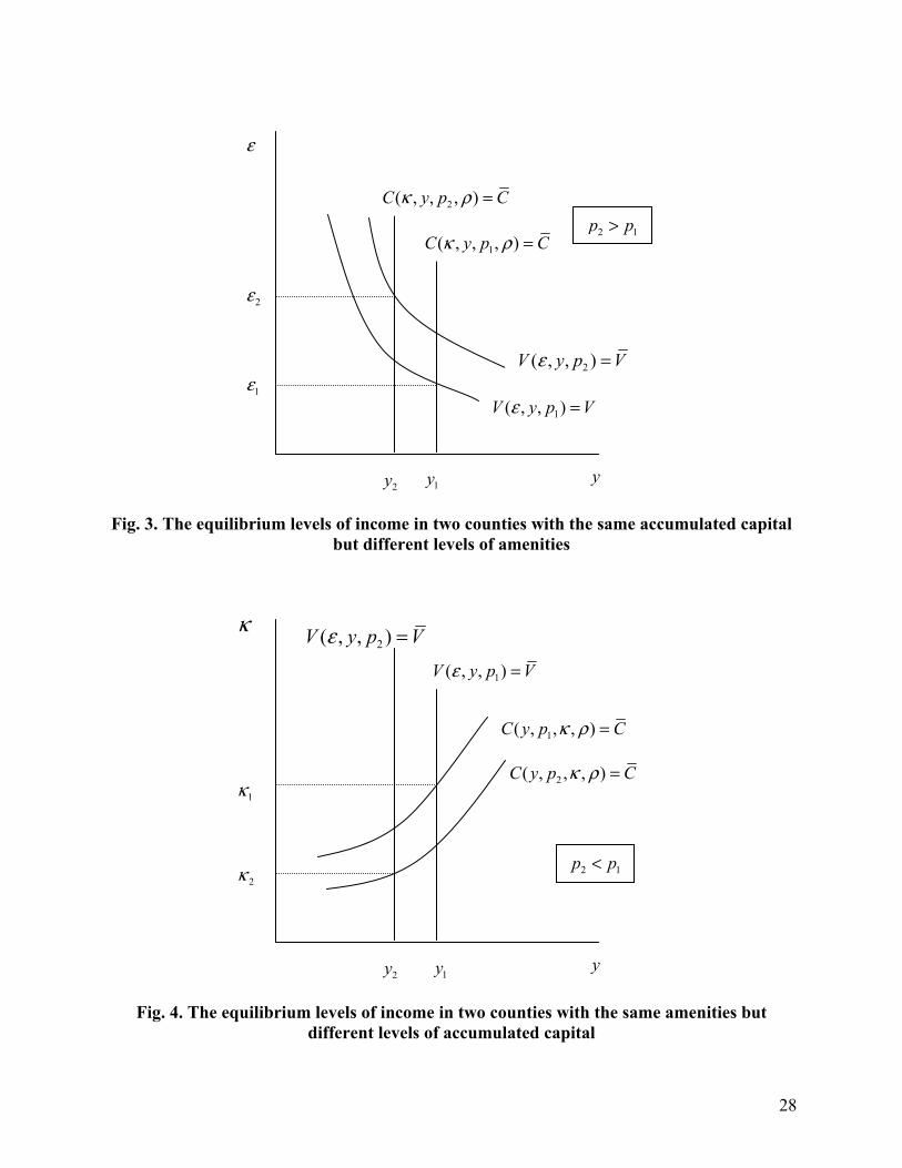
transportation costs, but county 1 has a lower level of amenities. Fig. 3 illustrates the
equilibrium levels of income and housing prices in the two counties. In Fig. 3, the relevant iso-
11
utility curve for households in county 1 is 1( , , )V y p Ve = , and the relevant iso-cost curve for
firms in county 1 is 1( , , , )C y p Ck r = . The iso-cost curves for firms are vertical in the ( , )ye -
plane because the firm's production cost is affected by y but not by e . Given the level of
amenities in county 1, 1e , the equilibrium income and housing price in county 1 will be 1y and
1p , respectively. Using county 1 as a reference point, consider the equilibrium level of housing
price and income in county 2. Because the level of amenities in county 2 is higher, the housing
price in county 2 must be higher. Otherwise, county 2 would have a lower housing price and a
higher level of amenities. This would imply that county 2 must have lower income in equilibrium
to ensure same utility for households living in the two counties. However, this could not be an
equilibrium for the firms because county 2 has both lower wage rates and lower rental costs.
Thus, in equilibrium, the housing price in county 2 must be higher than in county 1, which
implies that the iso-utility curve for county 2 is located above the iso-utility curve for county 1,
and the iso-cost curve for county 2 is located to the left of the iso-cost curve for county 1. In
equilibrium, county 2 (with a higher level of amenities) has lower income and higher housing
prices than county 1. In county 2, households trade lower income for higher amenities, and firms
trade a higher rental cost for lower wage rates.
Accumulated Capital and Economic Development
To analyze the effect of accumulated capital on the equilibrium level of income and housing
price, consider two counties that have the same level of natural endowments and transportation
costs, but county 1 has a higher level of accumulated human or physical capital. Fig. 4 illustrates
the equilibrium levels of income and housing prices in the two counties. In this case, the iso-
utility curves are vertical in the ( , )yk plane, but the iso-cost curves are upward sloping. In
12
equilibrium, housing prices in county 2 are lower than housing prices in county 1. The iso-cost
curve for county 1 is above the iso-cost curve for county 2. The iso-utility curve for county 1 is
located to the right of the iso-utility curve for county 2. The county with higher level of
accumulated capital will have higher income and housing prices than the county with lower level
of accumulated capital.
Remoteness and Economic Development
The effect of economic geography on economic development can be similarly analyzed as the
effect of accumulated capital. Consider two counties that have the same level of natural
endowments and accumulated capital, but county 2 is located in a more remote area than county
1. The relative levels of income and housing prices in the two counties can be illustrated using
figure 4 if we assume that a higher level of k represents less remoteness (i.e., lower r ). As
shown by the figure, county 2 (i.e., the county located in the remote area) will have lower
income and lower housing prices than county 1. This result supports the argument that
communities locating in a remote area have a disadvantage for economic development.
In sum, variations in income and housing prices across counties can be explained by the
spatial variation in natural endowments, accumulated human and physical capital, and economic
geography. Counties with more accumulated human or physical capital and a low level of
environmental amenities and transportation costs (i.e., some metro counties) will have a high
level of income in equilibrium, while counties with a low level of accumulated human or
physical capital and a high level of environmental amenities and transportation costs (i.e., some
rural counties) will have a low level of income. Housing prices in those two types of counties
depend on the relative magnitude of the amenity, capital, and location effects. In contrast,
counties with a high level of capital and amenities and low transportation costs (e.g., some

13
suburban counties) will have higher housing prices, while counties with a low level of capital
and amenities and high transportation costs (rural counties) will have lower housing prices.
Income in those types of counties will depend on the relative magnitude of the amenity, capital,
and location effects. These results are illustrated in Fig. 5.
Although the stylized model outlined above omits any direct representation of public
policies, it has some important implications on certain exogenously imposed rural development
policies. For example, our results suggest that public investments in rural infrastructure or
training of rural labor force can be an effective policy for promoting rural development. With
improvements in rural infrastructure, firms are more likely to be located in rural areas, which
may lead to higher income and higher housing prices in rural communities. Our results also
suggest that conservation to increase amenities in central city communities may not be an
effective policy to reduce poverty in inner city communities. Improving amenities in inner city
communities may attract some higher income households to those communities, but does not
create incentive for firms to provide jobs in those communities. Firms are willing to locate in
those communities only when households are willing to accept lower wages in exchange for the
improved amenities.
Empirical Model
Equations (3), (6), (8) and (9) describe the demand and supply sides of labor and land markets as
affected by natural endowments, accumulated human and physical capital, and economic
geography. These equations provide the theoretical basis for our empirical analysis of the effect
of natural endowments, accumulated human and physical capital, and economic geography on
economic development across counties in the U.S. Assuming the double-log functional form, the
demand and supply functions of labor and land development are empirically specified as follows:
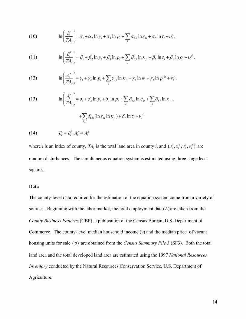
14
(10) 1 2 3 4 5ln ln ln ln lns
sii i k ki i i
ki
L y pTA
α α α α ε α τ υ
= + + + + +
∑ ,
(11) 1 2 3 4 5 6ln ln ln ln ln lnd
dii i j ji i i i
ji
L y pTA
β β β β κ β τ β ρ υ
= + + + + + +
∑ ,
(12) 1 2 3 4 5ln ln ln ln lns
ag sii j ji i i i
ji
A p w pTA
γ γ γ κ γ γ ν
= + + + + +
∑ ,
(13) 1 2 3 4 5ln ln ln ln lndi
i i k ki j jik ji
A y pTA
δ δ δ δ ε δ κ
= + + + +
∑ ∑ ,
6 7,
(ln ln ) ln dkj ki ji i i
k jδ ε κ δ τ ν+ + +∑
(14) ,s d s di i i iL L A A= =
where i is an index of county, iTA is the total land area in county i, and ( , , , )s d s di i i iυ υ ν ν are
random disturbances. The simultaneous equation system is estimated using three-stage least
squares.
Data
The county-level data required for the estimation of the equation system come from a variety of
sources. Beginning with the labor market, the total employment data ( )L are taken from the
County Business Patterns (CBP), a publication of the Census Bureau, U.S. Department of
Commerce. The county-level median household income (y) and the median price of vacant
housing units for sale ( )p are obtained from the Census Summary File 3 (SF3). Both the total
land area and the total developed land area are estimated using the 1997 National Resources
Inventory conducted by the Natural Resources Conservation Service, U.S. Department of
Agriculture.
15
The exogenous variables are broadly grouped into three categories: amenities ( )ε ,
physical and human capital/infrastructure ( )κ , and locational characteristics ( )ρ . The amenity
variables used in this study are generated using data from National Outdoor Recreation Supply
Information System (NORSIS), USDA Forest Service’s Wilderness Assessment Unit, Southern
Research Station, Athens, Georgia. The NORSIS is a comprehensive county level data set with
more than 250 amenity variables. We compiled the amenity variables into three indexes: climate
1( )ε , recreation 2( )ε , and water 3( )ε resources. To obtain these indexes, we use principal
component analysis to compress higher dimension variables in each category into a single scalar.
The single scalar is called a score, which is a the linear combination of the original variables,
where the linear weights are the eigenvectors of the correlation matrix between the set of factor
variables. Since the principal component is very sensitive to scale, all variables used in the
principal component analysis are standardized to zero mean and unit variance. The final score or
index equals1
M
mmm
xλ=∑ , where mλ is the eigenvector computed from the variance-covariance
matrix of the original data, mx is the standardized amenity variables and M is the number of
variables in a category.
For κ , physical capital data include road and lane miles, and the number of firms. Data
on road and lane miles 1( )κ are from the Bureau of Transportation Statistics, U.S. Department of
Commerce. Data on firms by employment size are from CBP, which are used to construct a
weighted average of the number of firms 2( )κ . Human capital 3( )κ is the share of bachelor-
degree holders in the labor force, which is obtained from SF3.
The location characteristics ( )ρ are represented by a set of county-level urban influence
categories developed by the Economic Research Service, U.S. Department of Agriculture. The
16
urban influence codes divide the counties in the United States into 12 groups. Metro counties are
divided into two groups by the size of the metro area—those in large areas with at least 1 million
residents and those in areas with fewer than 1 million residents. Nonmetro, micropolitan counties
are divided into three groups by their adjacency to metro areas—adjacent to a large metro area,
adjacent to a small metro area, and not adjacent to a metro area. Nonmetro, noncore counties are
divided into seven groups by their adjacency to metro or micro areas and whether or not they
have their own town of at least 2,500 residents. Hence, the urban influence code takes on values
1 through 12 with higher values indicating remoteness.
Data related to county governments, which serve as controls in our model are obtained
from the Census of Governments complied by the U.S. Census Bureau. For instance, public
education, health and safety expenditures are available to compute their shares in total public
expenditures by county. Moreover, the ratio of median real estate taxes and median housing
value, both from SF3, are used to represent the median property tax rate ( )τ of a county. To
reflect variations in costs of land development, wage rates in the construction sector (w), and
farmland prices ( agp ) are included in the supply equation of land development. The wage rates
in the construction sector (w) are obtained from CBP, and the farmland prices are obtained from
Lobowski, Plantinga, and Stavings (2003). Table 1 presents the summary statistics of all
variables used in the empirical analysis.
Results
The equation system (10)-(14) is estimated using the data described in the last section. The
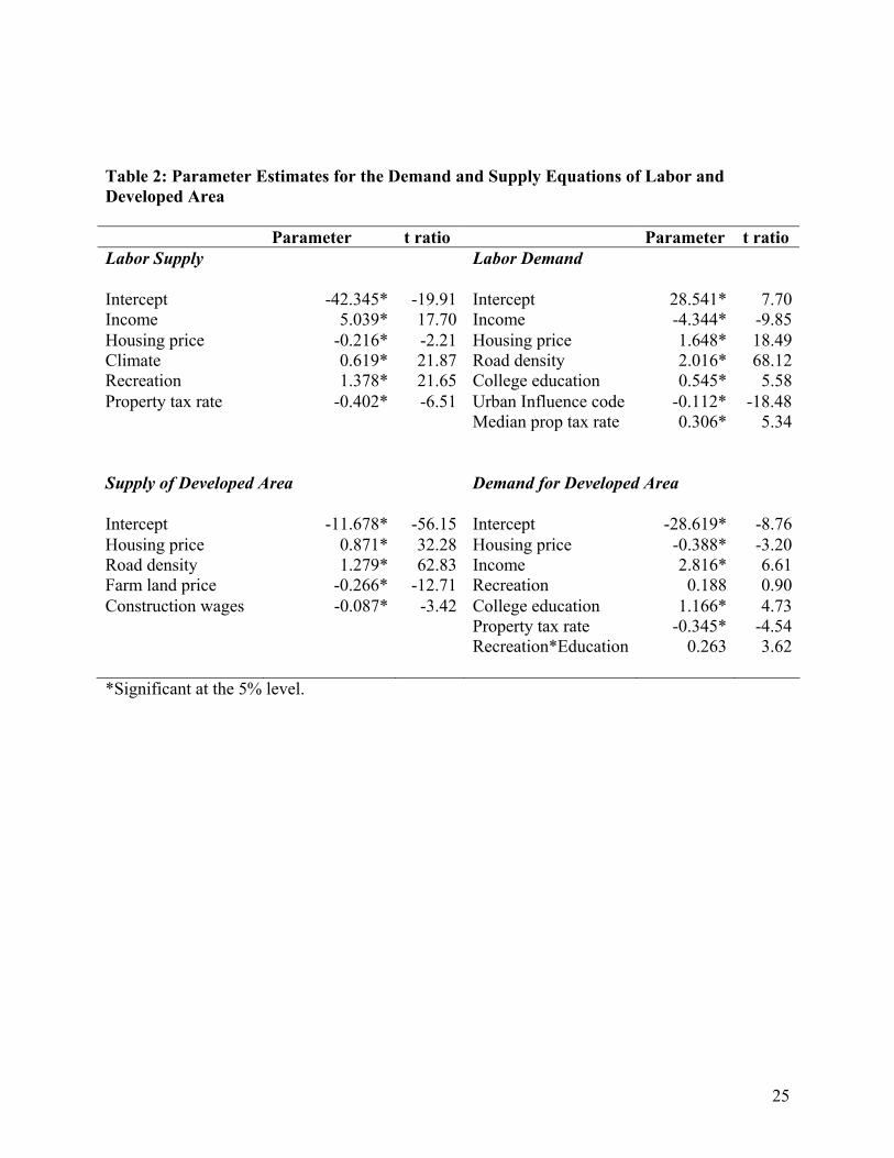
estimated coefficients are reported in table 2. Overall, the models fit the data well, with a
system-weighted R-square 0.75. Almost all coefficients are statistically significant at the 5%
level. Because the double-log functional form is used, the coefficients directly measure the

17
elesticities of demand and supply with respect to the corresponding variables.
The upper part of table 2 reports the labor supply and demand equations. As expected,
income is highly significant in both the demand and supply equations of labor. An increase in
income will increase the supply of labor, but reduce the demand for labor. Climate and
recreational opportunities are two measures of amenities and natural endowments. Consistent
with the theory, both are positive and statistically significant in the labor supply equation. This
implies that counties with mild climate and more recreational opportunities will attract more
labor. Likewise, accumulated physical and human capital, as measured by road density and the
percent of population with college education, are positive and highly significant in the labor
demand equation. This implies that counties with more accumulated human and physical capital
will attract more firms and thus have a high demand for labor. Remoteness, as measured by
urban influence code, is also statistically significant in the labor demand equation. Counties
located in remote areas are less attractive for firms and thus have lower demand for labor.
Housing prices and property taxes also affect labor demand and supply. As expected,
higher housing prices and higher property taxes reduce the supply of labor. However, the
positive effect of housing prices and property taxes on labor demand is less intuitive. Housing
prices and property taxes are included in the labor demand function to measure the cost of
factory space. An increase in the cost of factory space in a county may have two effects. First, it
may reduce the total number of firms located in the county because of higher production costs.
Second, it may cause both input substitutions within a firm and exit/entry of firms to the county.
As the cost of factory space increases, space-intensive firms may move out of the county, while
some labor-intensive firms may move into the county. Firms that stay in the county may
substitute some labor for factory space. The net effect of increasing housing prices on labor

18
demand will depend on the relative magnitude of the intensive and extensive marginal effects.
The positive signs on the housing price and property tax rate in the labor demand equation imply
that the intensive marginal effect dominates.
Table 2 also reports the estimated coefficients of the demand and supply equations of
land development. As expected, an increase in housing price increases the supply of developed
area, while an increase in the production costs as measured by farmland prices and construction
wage rates reduces the supply of developed area. The demand for developed land is significantly
affected by housing price, income, amenities, and accumulated human capital. A 1% increase in
housing price reduces total demand for developed areas by 0.39%. The demand for developed
land is much more responsive to income and accumulated human capital than to housing prices.
A 1% increase in income and the percent of population with college education will increase the
demand for housing by 2.8% and 1.2%, respectively.
Amenities, Capital, Geography, and Spatial Variations in Economic Development
The interactions between the location decisions of firms and households shape the labor and land
markets and determine economic development across the counties. Because in most cases,
natural endowment, accumulated human and physical capital, and remoteness affect both the
firm and household decisions, either directly or indirectly, the final effect of these factors on
communities depends on the relative magnitudes of their effects on the demand and supply of
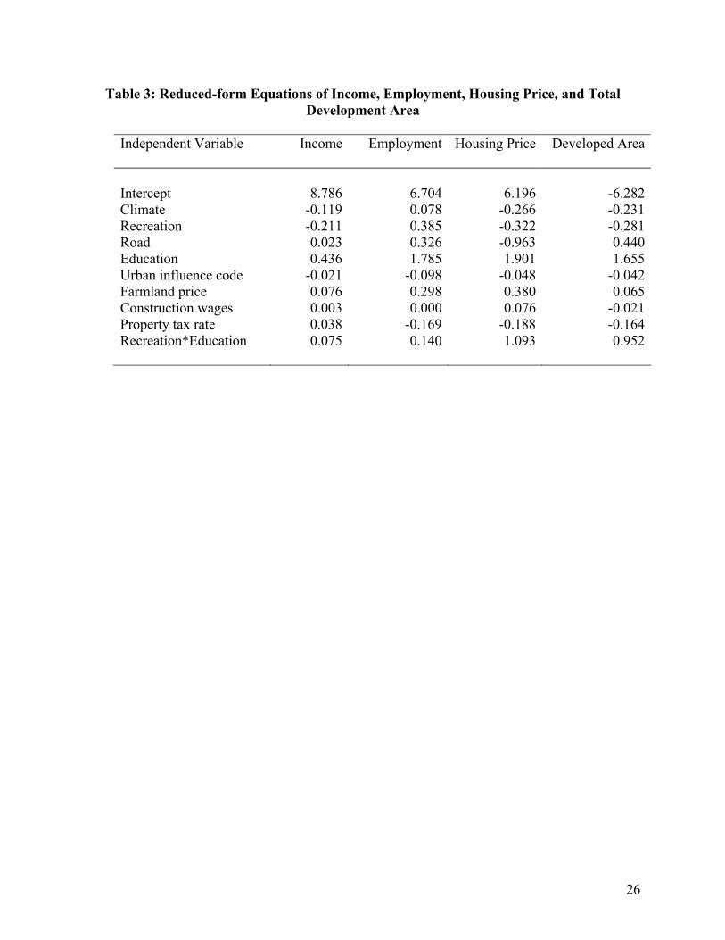
labor and land development. To evaluate the final effects, we derive the reduced-form equations
of income, employment, housing prices, and total developed area as functions of these factors
from the structural equations. The results are reported in table 3. Because the double-log
functional form is used, the coefficients measure the elasticities of income, employment, housing
price, and total developed area with respect to these exogenous variables in equilibrium.
19
Results suggest that counties with better climate and more creational opportunities have
lower income and more employment opportunities in equilibrium. This implies that households
are willing to trade better amenities for lower wages. Firms take advantage of households'
willingness to accept lower wages by locating in those counties with better climate and more
recreational opportunities. Because of lower income, counties with better amenities have lower
housing prices and less developed area in equilibrium. Counties with more accumulated human
and physical capital, as measured by road density and percent of population with college
education, have higher income, more employment opportunities, and high development density.
However, high road density reduces housing prices, although more accumulated human capital
raises housing prices. Remoteness, as measured by urban influence code, has a negative effect on
every measure of economic development indicator. It reduces income, employment, housing
prices and total developed areas.
Conclusions
This article evaluates the contributions of natural endowments, accumulated human and physical
capital, and economic geography to the spatial inequalities of economic development in rural
America. A theoretical model is developed to analyze the interrelationship between location
decisions of firms and households as they are affected by natural endowments, accumulated
capital, and economic geography. Based on the theoretical analysis, an empirical model is
specified and estimated to quantify the effect of natural endowments, accumulated capital, and
economic geography on the spatial distribution of economic activities across counties in the
United States. Preliminary results suggest that households are willing to trade better amenities
for lower income, and firms take advantage of this by locating in areas with better climate and
more recreational opportunities. In equilibrium, counties with better climate and more creational

20
opportunities have lower income and more employment opportunities. Because of lower income
in those counties, counties with better amenities have lower housing prices and less developed
area in equilibrium. Likewise, accumulated human and physical capital also significantly affect
economic development across counties in the United States. Counties with more accumulated
human and physical capital have higher income, more employment opportunities, and high
development density. However, high road density reduces housing prices. Remoteness, as
measured by urban influence code, has a negative effect on every measure of economic
development indicator. It reduces income, employment, housing prices and total developed
areas. The results increase our understanding of causes of spatial inequalities in economic
development and provide information for policy development to promote community vitality and
economic prosperity in rural America.
21
References Bradford, D., W. E. Oates, "Suburban Exploitation of Central Cities and Government Structure,"
in Hochman, H, and Peterson, G. (eds.), Redistribution Through Public Choice, New York: Columbia University Press, 1974.
Brueckner, J. K., T. Jacques-Francois, Y. Zenou, “Why Is Central Paris Rich and Downtown
Detroit Poor? An Amenity-Based Theory,” European Economic Review, 43 (1999), 91-107.
Castle, E. N., The Changing American Countryside: Rural People and Places, Lawrence, Kansas:
The University Press of Kansas, 1995. Deller, S. C., T.-H. Tsai, D. W. Marcouiller, and D. B. K. English, "The Role of Amenities and
Quality of Life in Rural Economic Growth," American Journal of Agricultural Economics, 83 (2001), 352-365.
Dissart, J. C., and S. C. Deller, "Quality of Life on the Planning Literature," Journal of Planning
Literature, 15 (2000), 135-161. Economic Research Services, U.S. Department of Agriculture. Briefing Room: Rural Income,
Poverty, and Welfare. Washington DC, 2004. Epple, D., T. Romer, “Mobility and Redistribution,” Journal of Political Economy, 99 (1991),
828-58. Epple, D., H. Sieg, “Estimating Equilibrium Models of Local Jurisdictions,” Journal of Political
Economy, 107 (1999), 645-681. Fernandez, R., R. Rogerson, "Income Distribution, Communities, and the Quality of Public
Education," Quarterly Journal of Economics,111 (1996), 135-64. Fujita, M., P. Krugman, and A. J. Venables, Spatial Economy; Cities, Regions, and International
Trade, Cambridge, MA: MIT Press, 1999. Gallup, J. L., and J. Sachs, "Geography and Economic Development," in B. Plseskovic and J.E.
Stiglitz (eds) Annual Bank Conference on Development Economics. Washington DC: World Bank.
Geoghegan, J., L. A. Wainger, and N. E. Bockstael, “Spatial Landscape Indices in a Hedonic
Framework: An Ecological Economics Analysis Using GIS.” Ecological Economics, 23 (1997), 251-64.
Giannias, D. A., and P. G. Liargovas, "Firm and Household Mobility in the presence of
variations in Regional Characteristics," Regional Science, 36(2002), 299-313.
22
Gopinath, M., and R. Echeverria, “Does Economic Development Impact the Foreign Direct Investment-Trade Relationship? A Gravity Model Approach,” American Journal of Agricultural Economics, 86 (2004), 782-787. Gopinath, M., D. Pick and Y. Li, “An Empirical Analysis of Productivity Growth and Industrial Concentration in U.S. Manufacturing.” Applied Economics, 36(2004), 1-7. Gopinath, M., and W. Chen, “Foreign Direct Investment and Wages: A Cross-Country Analysis.” Journal of International Trade and Economic Development, 12(2003), 285- 309. Gottlieb, P. D., "Amenities as an Economic Development Tool: Is there Enough Evidence?,"
Economic Development Quarterly, 8 (1994), 270-85. Halstead, J. M., and S. C. Deller, "Public Infrastructure in Economic Development and Growth:
Evidence from Rural Manufacturers," Journal of Community Development Society, 28 (1997), 149-69.
Henderson, J. V., Z. Shalizi, and A. J. Venables, "Geography and Development." Journal of
Economic Geography, 1 (2001),81-105. Irwin, E. G., N. E. Bockstael, “Interacting Agents, Spatial Externalities, and the Evolution of
Residential Land Use Patterns,” Journal Economic Geography, 2 (2002), 31-54. Krugman, P., “Increasing Returns and Economic Geography,” Journal of Political Economy, 99
(1991), 438-99. LeRoy, S., J. Sonstelie, “Paradise Lost and Regained: Transportation Innovation, Income, and
Residential Segregation,” Journal of Urban Economics,13 (1983), 67-89. Lubowski, R. N., A. J. Plantinga, and R. N. Stavins, 2003, Determinants of land-use change in
the United States, 1982-97: results from a national-level econometric and simulation analysis, Working paper, Economic Research Search, U.S. Department of Agriculture.
Rappaport, J. and J. D. Sachs, "The U.S. as a Coastal Nation," RWP 01-11, Research Division,
Federal Reserve Bank of Kansas City, 2002. Rainey, D.V., and K. T. McNamara, "Taxes and the Location Decision of Manufacturing
Establishments," Review of Agricultural Economics, 21(1999), 86-98. Redding, S. J., and A. J. Venables, Economic Geography and International Inequality,
Discussion Paper, Center for Economic Policy, London, 2000. Rudzitis, G., "Amenities Increasingly Drew People to the Rural West," Rural Development
Perspectives, 14 (1999), 23-28.

23
Tiebout, C. M., "The Theory of Urban Residential Location,” Journal of Political Economy, 64 (1956), 416-24.
Wheaton, W. C., “Income and Urban Residence: An Analysis of Consumer Demand for
Location,” American Economic Review, 67 (1977), 620-31. Wu, J., “Environmental Amenities and the Spatial Patterns of Urban Sprawl,” American Journal
of Agricultural Economics, 83(2001), 691-697. Wu, JunJie. “Amenities, Sprawls, and the Economic Landscape.” Paper presented in the Land
Markets and Regulation Seminar, Lincoln Institute of Land Policy, Cambridge, MA. July 10-12, 2002.
Wu, J., R. Adams, A. J. Plantinga, "Amenities in an Urban Equilibrium Model: Residential
Development in Portland, Oregon,” Land Economics, 80(February 2004), 19-32. Wu, J., and A. J. Plantinga. “The Influence of Public Open Space Policies on Urban Spatial
Structure,” Journal of Environmental Economics and Management, 46(September 2003), 288-309.

24
Table 1: Descriptive Statistics of County Data (2677 Counties) Name of Variable Unit Mean Standard
Deviation Minimum Maximum
Employment Number 44677 145939 434 4421930Income $ 36576 8759 17062 91210Developed area 1000 acres 32.7364 46.3656 1.5000 945.8000Housing price $ 68278 57610 9999 1000001Climate Index 0.5640 0.2187 0.0000 1.0000Recreation Index 0.0498 0.0364 0.0000 1.0000Road density Miles/acre 2.9738 2.0619 0.1282 26.4234College education % population 0.1097 0.0488 0.0247 0.4001Median property tax rate % 1.0475 0.4945 0.2163 3.1566Farmland price $/acre 1772 5368 87 242143Construction wages $/year 5714 1808 500 34950Urban influence code Index 5.3403 3.3877 1.0000 12.0000
25
Table 2: Parameter Estimates for the Demand and Supply Equations of Labor and Developed Area Parameter t ratio Parameter t ratio Labor Supply Labor Demand
Intercept -42.345* -19.91 Intercept 28.541* 7.70Income 5.039* 17.70 Income -4.344* -9.85Housing price -0.216* -2.21 Housing price 1.648* 18.49Climate 0.619* 21.87 Road density 2.016* 68.12Recreation 1.378* 21.65 College education 0.545* 5.58Property tax rate -0.402* -6.51 Urban Influence code -0.112* -18.48 Median prop tax rate 0.306* 5.34 Supply of Developed Area Demand for Developed Area
Intercept -11.678* -56.15 Intercept -28.619* -8.76Housing price 0.871* 32.28 Housing price -0.388* -3.20Road density 1.279* 62.83 Income 2.816* 6.61Farm land price -0.266* -12.71 Recreation 0.188 0.90Construction wages -0.087* -3.42 College education 1.166* 4.73
Property tax rate -0.345* -4.54 Recreation*Education 0.263 3.62
*Significant at the 5% level.
26
Table 3: Reduced-form Equations of Income, Employment, Housing Price, and Total Development Area
Independent Variable Income Employment Housing Price Developed Area
Intercept 8.786 6.704 6.196 -6.282Climate -0.119 0.078 -0.266 -0.231Recreation -0.211 0.385 -0.322 -0.281Road 0.023 0.326 -0.963 0.440Education 0.436 1.785 1.901 1.655Urban influence code -0.021 -0.098 -0.048 -0.042Farmland price 0.076 0.298 0.380 0.065Construction wages 0.003 0.000 0.076 -0.021Property tax rate 0.038 -0.169 -0.188 -0.164Recreation*Education 0.075 0.140 1.093 0.952
27
Fig. 1. Tradeoffs between income and amenities for households
Fig. 2. Tradeoffs between wage rates and accumulated capital for firms
y
e
1( , , )V y p Ve =2( , , )V y p Ve =
y
k 2( , , , )C y p Ck r =
1( , , , )C y p Ck r =
28
Fig. 3. The equilibrium levels of income in two counties with the same accumulated capital
but different levels of amenities
Fig. 4. The equilibrium levels of income in two counties with the same amenities but
different levels of accumulated capital
y
e
1( , , )V y p Ve =
1( , , , )C y p Ck r =
1y
1e 2( , , )V y p Ve =
2( , , , )C y p Ck r =
2y
2e
2 1p p>
y
k
1( , , )V y p Ve =
1( , , , )C y p Ck r =
1y
1k
2( , , )V y p Ve =
2( , , , )C y p Ck r =
2y
2k 2 1p p<

29
Fig. 5. Amenities, accumulated capital, and the spatial variation in income
and housing prices
e
k or ρ
Income: High Housing price: • High if the capital
effect dominates • Low if the amenity
effect dominate
Income: • High if the capital
effect dominates • Low if the amenity
effect dominate Housing price: High
Income: • High if the amenity
effect dominates • Low if the capital
effect dominate Housing price: Low
Income: Low Housing price: • High if the amenity
effect dominates • Low if the capital
effect dominate