How Does Batch Normalization Help Optimization?

How Does Batch Normalization Help Optimization?

Shibani Santurkar∗MIT

[email protected]

Dimitris Tsipras∗MIT

[email protected]

Andrew Ilyas∗MIT

[email protected]

Aleksander MadryMIT

[email protected]

Abstract

Batch Normalization (BatchNorm) is a widely adopted technique that enablesfaster and more stable training of deep neural networks (DNNs). Despite itspervasiveness, the exact reasons for BatchNorm’s effectiveness are still poorlyunderstood. The popular belief is that this effectiveness stems from controllingthe change of the layers’ input distributions during training to reduce the so-called“internal covariate shift”. In this work, we demonstrate that such distributionalstability of layer inputs has little to do with the success of BatchNorm. Instead,we uncover a more fundamental impact of BatchNorm on the training process: itmakes the optimization landscape significantly smoother. This smoothness inducesa more predictive and stable behavior of the gradients, allowing for faster training.

1 Introduction

Over the last decade, deep learning has made impressive progress on a variety of notoriouslydifficult tasks in computer vision [16, 7], speech recognition [5], machine translation [29], andgame-playing [18, 25]. This progress hinged on a number of major advances in terms of hardware,datasets [15, 23], and algorithmic and architectural techniques [27, 12, 20, 28]. One of the mostprominent examples of such advances was batch normalization (BatchNorm) [10].

At a high level, BatchNorm is a technique that aims to improve the training of neural networks bystabilizing the distributions of layer inputs. This is achieved by introducing additional network layersthat control the first two moments (mean and variance) of these distributions.

The practical success of BatchNorm is indisputable. By now, it is used by default in most deep learningmodels, both in research (more than 6,000 citations) and real-world settings. Somewhat shockingly,however, despite its prominence, we still have a poor understanding of what the effectiveness ofBatchNorm is stemming from. In fact, there are now a number of works that provide alternatives toBatchNorm [1, 3, 13, 31], but none of them seem to bring us any closer to understanding this issue.(A similar point was also raised recently in [22].)

Currently, the most widely accepted explanation of BatchNorm’s success, as well as its originalmotivation, relates to so-called internal covariate shift (ICS). Informally, ICS refers to the change inthe distribution of layer inputs caused by updates to the preceding layers. It is conjectured that suchcontinual change negatively impacts training. The goal of BatchNorm was to reduce ICS and thusremedy this effect.

Even though this explanation is widely accepted, we seem to have little concrete evidence supportingit. In particular, we still do not understand the link between ICS and training performance. The chiefgoal of this paper is to address all these shortcomings. Our exploration lead to somewhat startlingdiscoveries.

∗Equal contribution.

32nd Conference on Neural Information Processing Systems (NIPS 2018), Montréal, Canada.

arX

iv:1

805.

1160

4v3

[st

at.M

L]

27

Oct

201

8

Our Contributions. Our point of start is demonstrating that there does not seem to be any linkbetween the performance gain of BatchNorm and the reduction of internal covariate shift. Or that thislink is tenuous, at best. In fact, we find that in a certain sense BatchNorm might not even be reducinginternal covariate shift.

We then turn our attention to identifying the roots of BatchNorm’s success. Specifically, we demon-strate that BatchNorm impacts network training in a fundamental way: it makes the landscape ofthe corresponding optimization problem significantly more smooth. This ensures, in particular, thatthe gradients are more predictive and thus allows for use of larger range of learning rates and fasternetwork convergence. We provide an empirical demonstration of these findings as well as theirtheoretical justification. We prove that, under natural conditions, the Lipschitzness of both the lossand the gradients (also known as β-smoothness [21]) are improved in models with BatchNorm.

Finally, we find that this smoothening effect is not uniquely tied to BatchNorm. A number of othernatural normalization techniques have a similar (and, sometime, even stronger) effect. In particular,they all offer similar improvements in the training performance.

We believe that understanding the roots of such a fundamental techniques as BatchNorm will let ushave a significantly better grasp of the underlying complexities of neural network training and, inturn, will inform further algorithmic progress in this context.

Our paper is organized as follows. In Section 2, we explore the connections between BatchNorm,optimization, and internal covariate shift. Then, in Section 3, we demonstrate and analyze the exactroots of BatchNorm’s success in deep neural network training. We present our theoretical analysis inSection 4. We discuss further related work in Section 5 and conclude in Section 6.

2 Batch normalization and internal covariate shift

Batch normalization (BatchNorm) [10] has been arguably one of the most successful architecturalinnovations in deep learning. But even though its effectiveness is indisputable, we do not have a firmunderstanding of why this is the case.

Broadly speaking, BatchNorm is a mechanism that aims to stabilize the distribution (over a mini-batch) of inputs to a given network layer during training. This is achieved by augmenting the networkwith additional layers that set the first two moments (mean and variance) of the distribution of eachactivation to be zero and one respectively. Then, the batch normalized inputs are also typically scaledand shifted based on trainable parameters to preserve model expressivity. This normalization isapplied before the non-linearity of the previous layer.

One of the key motivations for the development of BatchNorm was the reduction of so-called internalcovariate shift (ICS). This reduction has been widely viewed as the root of BatchNorm’s success.Ioffe and Szegedy [10] describe ICS as the phenomenon wherein the distribution of inputs to a layerin the network changes due to an update of parameters of the previous layers. This change leads to aconstant shift of the underlying training problem and is thus believed to have detrimental effect onthe training process.

0 5k 10k 15kSteps

50

100

Trai

ning

Acc

urac

y (%

)

Standard, LR=0.1Standard + BatchNorm, LR=0.1Standard, LR=0.5Standard + BatchNorm, LR=0.5

0 5k 10k 15kSteps

50

100

Test

Acc

urac

y (%

)

Standard, LR=0.1Standard + BatchNorm, LR=0.1Standard, LR=0.5Standard + BatchNorm, LR=0.5

Laye

r #3

Standard Standard + BatchNorm

Laye

r #11

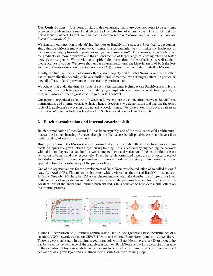
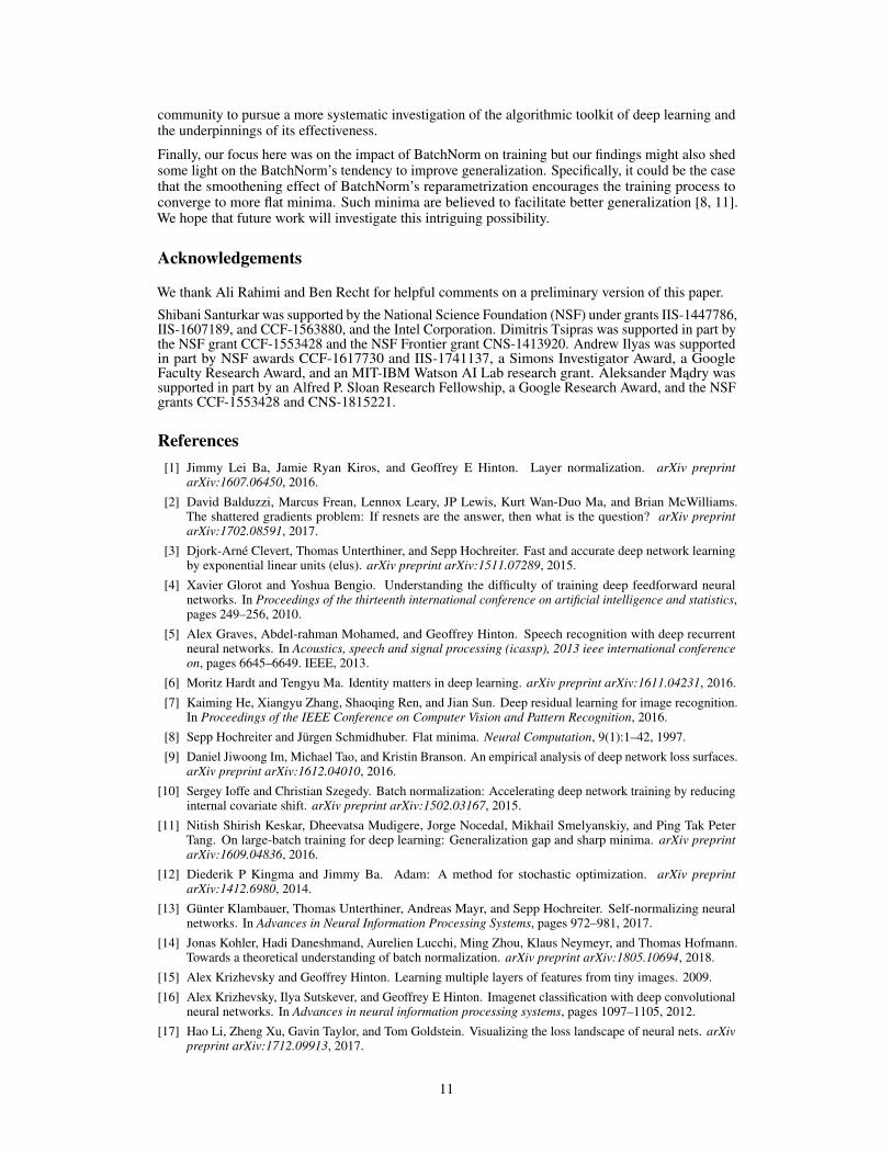
Figure 1: Comparison of (a) training (optimization) and (b) test (generalization) performance of astandard VGG network trained on CIFAR-10 with and without BatchNorm (details in Appendix A).There is a consistent gain in training speed in models with BatchNorm layers. (c) Even though thegap between the performance of the BatchNorm and non-BatchNorm networks is clear, the differencein the evolution of layer input distributions seems to be much less pronounced. (Here, we sampledactivations of a given layer and visualized their distribution over training steps.)

2

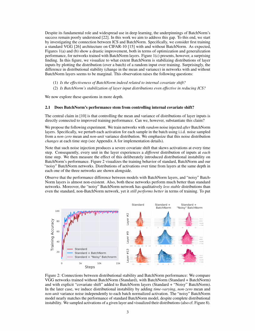
Despite its fundamental role and widespread use in deep learning, the underpinnings of BatchNorm’ssuccess remain poorly understood [22]. In this work we aim to address this gap. To this end, we startby investigating the connection between ICS and BatchNorm. Specifically, we consider first traininga standard VGG [26] architecture on CIFAR-10 [15] with and without BatchNorm. As expected,Figures 1(a) and (b) show a drastic improvement, both in terms of optimization and generalizationperformance, for networks trained with BatchNorm layers. Figure 1(c) presents, however, a surprisingfinding. In this figure, we visualize to what extent BatchNorm is stabilizing distributions of layerinputs by plotting the distribution (over a batch) of a random input over training. Surprisingly, thedifference in distributional stability (change in the mean and variance) in networks with and withoutBatchNorm layers seems to be marginal. This observation raises the following questions:

(1) Is the effectiveness of BatchNorm indeed related to internal covariate shift?(2) Is BatchNorm’s stabilization of layer input distributions even effective in reducing ICS?

We now explore these questions in more depth.

2.1 Does BatchNorm’s performance stem from controlling internal covariate shift?

The central claim in [10] is that controlling the mean and variance of distributions of layer inputs isdirectly connected to improved training performance. Can we, however, substantiate this claim?

We propose the following experiment. We train networks with random noise injected after BatchNormlayers. Specifically, we perturb each activation for each sample in the batch using i.i.d. noise sampledfrom a non-zero mean and non-unit variance distribution. We emphasize that this noise distributionchanges at each time step (see Appendix A for implementation details).

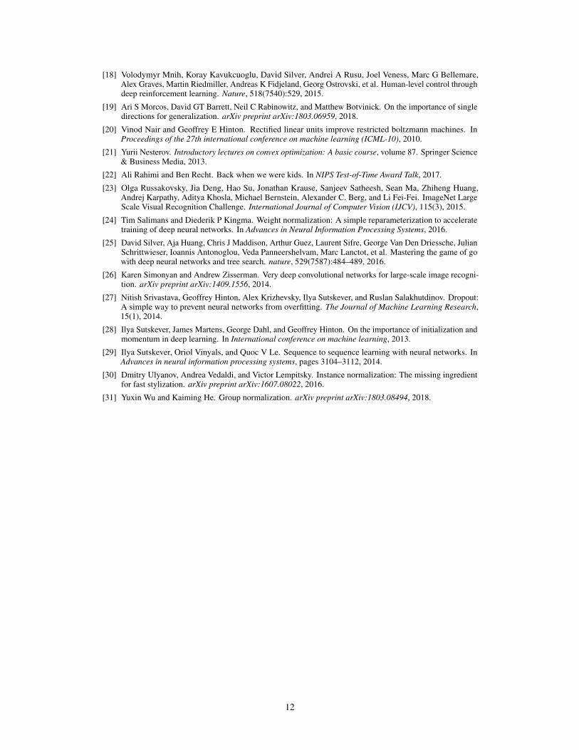
Note that such noise injection produces a severe covariate shift that skews activations at every timestep. Consequently, every unit in the layer experiences a different distribution of inputs at eachtime step. We then measure the effect of this deliberately introduced distributional instability onBatchNorm’s performance. Figure 2 visualizes the training behavior of standard, BatchNorm and our“noisy” BatchNorm networks. Distributions of activations over time from layers at the same depth ineach one of the three networks are shown alongside.

Observe that the performance difference between models with BatchNorm layers, and “noisy” Batch-Norm layers is almost non-existent. Also, both these networks perform much better than standardnetworks. Moreover, the “noisy” BatchNorm network has qualitatively less stable distributions thaneven the standard, non-BatchNorm network, yet it still performs better in terms of training. To put

0 5k 10k 15kSteps

20

40

60

80

100

Trai

ning

Acc

urac

y

StandardStandard + BatchNormStandard + "Noisy" Batchnorm

Laye

r #2

Standard Standard + BatchNorm

Standard + "Noisy" BatchNorm

Laye

r #9

Laye

r #13

Figure 2: Connections between distributional stability and BatchNorm performance: We compareVGG networks trained without BatchNorm (Standard), with BatchNorm (Standard + BatchNorm)and with explicit “covariate shift” added to BatchNorm layers (Standard + “Noisy” BatchNorm).In the later case, we induce distributional instability by adding time-varying, non-zero mean andnon-unit variance noise independently to each batch normalized activation. The “noisy” BatchNormmodel nearly matches the performance of standard BatchNorm model, despite complete distributionalinstability. We sampled activations of a given layer and visualized their distributions (also cf. Figure 8).

3

20

40

60

80

100

Trai

ning

Acc

urac

y (%

)LR

= 0

.1LR

= 0

.1

StandardStandard + BatchNorm

0 5k 10k 15kSteps

20

40

60

80

100Tr

aini

ng A

ccur

acy

(%)

LR =

0.0

1LR

= 0

.01


10 2

100

2-diff

eren

ce

Layer #5

0

1

Cos A

ngle

Layer #10

10 3

10 1

101

2-diff

eren

ce

0 5k 10k 15kSteps

0

1

Cos A

ngle

0 5k 10k 15kSteps

(a) VGG

103

104

Trai

ning

Los

sLR

= 1

e-06

LR =

1e-

06


0 5k 10kSteps

103

104

Trai

ning

Los

sLR

= 1

e-07

LR =

1e-

07


102

103

104

2-Diff

eren

ce

Layer #9

0

1

Cos A

ngle

Layer #17

101

103

2-Diff

eren

ce

0 5k 10kSteps

0

1

Cos A

ngle

0 5k 10kSteps

(b) DLN

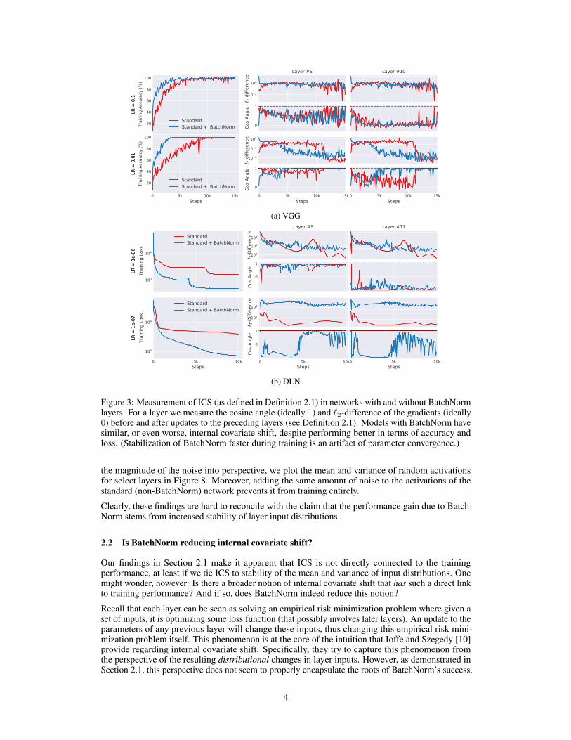
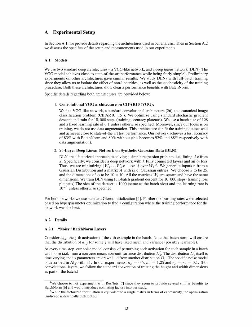
Figure 3: Measurement of ICS (as defined in Definition 2.1) in networks with and without BatchNormlayers. For a layer we measure the cosine angle (ideally 1) and `2-difference of the gradients (ideally0) before and after updates to the preceding layers (see Definition 2.1). Models with BatchNorm havesimilar, or even worse, internal covariate shift, despite performing better in terms of accuracy andloss. (Stabilization of BatchNorm faster during training is an artifact of parameter convergence.)

the magnitude of the noise into perspective, we plot the mean and variance of random activationsfor select layers in Figure 8. Moreover, adding the same amount of noise to the activations of thestandard (non-BatchNorm) network prevents it from training entirely.

Clearly, these findings are hard to reconcile with the claim that the performance gain due to Batch-Norm stems from increased stability of layer input distributions.

2.2 Is BatchNorm reducing internal covariate shift?

Our findings in Section 2.1 make it apparent that ICS is not directly connected to the trainingperformance, at least if we tie ICS to stability of the mean and variance of input distributions. Onemight wonder, however: Is there a broader notion of internal covariate shift that has such a direct linkto training performance? And if so, does BatchNorm indeed reduce this notion?

Recall that each layer can be seen as solving an empirical risk minimization problem where given aset of inputs, it is optimizing some loss function (that possibly involves later layers). An update to theparameters of any previous layer will change these inputs, thus changing this empirical risk mini-mization problem itself. This phenomenon is at the core of the intuition that Ioffe and Szegedy [10]provide regarding internal covariate shift. Specifically, they try to capture this phenomenon fromthe perspective of the resulting distributional changes in layer inputs. However, as demonstrated inSection 2.1, this perspective does not seem to properly encapsulate the roots of BatchNorm’s success.

4

To answer this question, we consider a broader notion of internal covariate shift that is more tied tothe underlying optimization task. (After all the success of BatchNorm is largely of an optimizationnature.) Since the training procedure is a first-order method, the gradient of the loss is the most naturalobject to study. To quantify the extent to which the parameters in a layer would have to “adjust” inreaction to a parameter update in the previous layers, we measure the difference between the gradientsof each layer before and after updates to all the previous layers. This leads to the following definition.

Definition 2.1. Let L be the loss, W (t)1 , . . . , W (t)

k be the parameters of each of the k layers and(x(t), y(t)) be the batch of input-label pairs used to train the network at time t. We define internalcovariate shift (ICS) of activation i at time t to be the difference ||Gt,i −G′t,i||2, where

Gt,i = ∇W (t)iL(W (t)

1 , . . . ,W(t)k ;x(t), y(t))

G′t,i = ∇W (t)iL(W (t+1)

1 , . . . ,W(t+1)i−1 ,W

(t)i ,W

(t)i+1, . . . ,W

(t)k ;x(t), y(t)).

Here, Gt,i corresponds to the gradient of the layer parameters that would be applied during asimultaneous update of all layers (as is typical). On the other hand, G′t,i is the same gradient after allthe previous layers have been updated with their new values. The difference between G and G′ thusreflects the change in the optimization landscape of Wi caused by the changes to its input. It thuscaptures precisely the effect of cross-layer dependencies that could be problematic for training.

Equipped with this definition, we measure the extent of ICS with and without BatchNorm layers. Toisolate the effect of non-linearities as well as gradient stochasticity, we also perform this analysis on(25-layer) deep linear networks (DLN) trained with full-batch gradient descent (see Appendix A fordetails). The conventional understanding of BatchNorm suggests that the addition of BatchNormlayers in the network should increase the correlation between G and G′, thereby reducing ICS.

Surprisingly, we observe that networks with BatchNorm often exhibit an increase in ICS (cf. Figure 3).This is particularly striking in the case of DLN. In fact, in this case, the standard network experiencesalmost no ICS for the entirety of training, whereas for BatchNorm it appears that G and G′ arealmost uncorrelated. We emphasize that this is the case even though BatchNorm networks continue toperform drastically better in terms of attained accuracy and loss. (The stabilization of the BatchNormVGG network later in training is an artifact of faster convergence.)

This evidence suggests that, from optimization point of view, controlling the distributions layer inputsas done in BatchNorm, might not even reduce the internal covariate shift.

3 Why does BatchNorm work?

Our investigation so far demonstrated that the generally asserted link between the internal covariateshift (ICS) and the optimization performance is tenuous, at best. But BatchNorm does significantlyimprove the training process. Can we explain why this is the case?

Aside from reducing ICS, Ioffe and Szegedy [10] identify a number of additional properties ofBatchNorm. These include prevention of exploding or vanishing gradients, robustness to differentsettings of hyperparameters such as learning rate and initialization scheme, and keeping most of theactivations away from saturation regions of non-linearities. All these properties are clearly beneficialto the training process. But they are fairly simple consequences of the mechanics of BatchNormand do little to uncover the underlying factors responsible for BatchNorm’s success. Is there a morefundamental phenomenon at play here?

3.1 The smoothing effect of BatchNorm

Indeed, we identify the key impact that BatchNorm has on the training process: it reparametrizesthe underlying optimization problem to make its landscape significantly more smooth. The firstmanifestation of this impact is improvement in the Lipschitzness2 of the loss function. That is, theloss changes at a smaller rate and the magnitudes of the gradients are smaller too. There is, however,

2Recall that f is L-Lipschitz if |f(x1)− f(x2)| ≤ L‖x1 − x2‖, for all x1 and x2.

5

0 5k 10k 15kSteps

100

101

Loss

Lan

dsca

pe


(a) loss landscape

0 5k 10k 15kSteps

0

50

100

150

200

250

Grad

ient

Pre

dict

iven

ess Standard

Standard + BatchNorm

(b) gradient predictiveness

0 5k 10k 15kSteps

5

10

15

20

25

30

35

40

45

-sm

ooth

ness


(c) “effective” β-smoothness

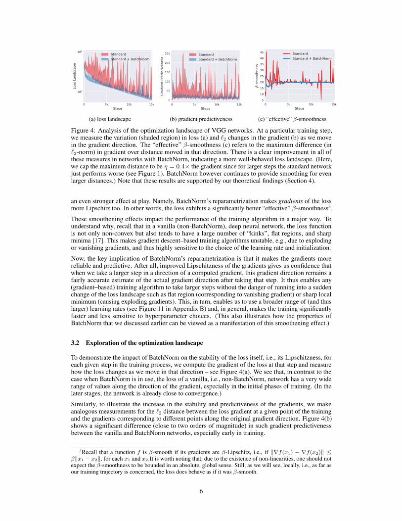
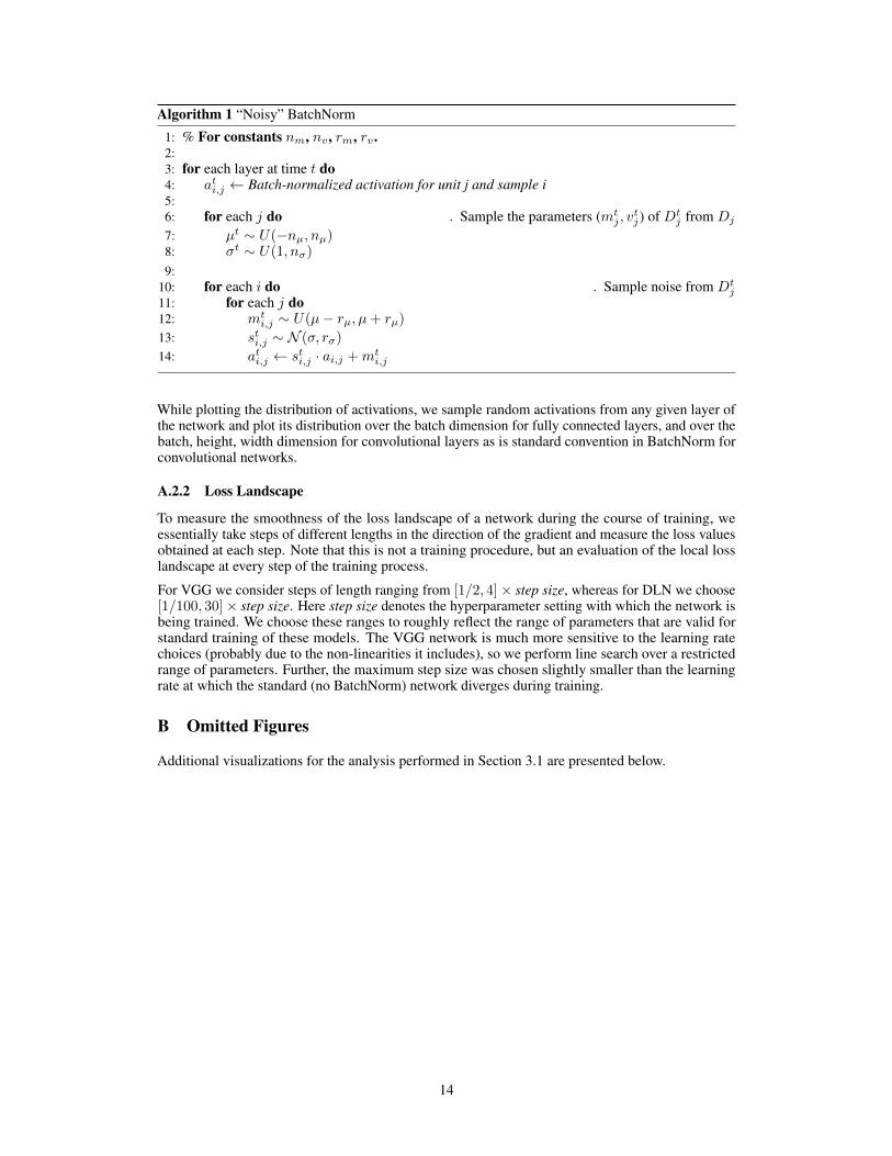
Figure 4: Analysis of the optimization landscape of VGG networks. At a particular training step,we measure the variation (shaded region) in loss (a) and `2 changes in the gradient (b) as we movein the gradient direction. The “effective” β-smoothness (c) refers to the maximum difference (in`2-norm) in gradient over distance moved in that direction. There is a clear improvement in all ofthese measures in networks with BatchNorm, indicating a more well-behaved loss landscape. (Here,we cap the maximum distance to be η = 0.4× the gradient since for larger steps the standard networkjust performs worse (see Figure 1). BatchNorm however continues to provide smoothing for evenlarger distances.) Note that these results are supported by our theoretical findings (Section 4).

an even stronger effect at play. Namely, BatchNorm’s reparametrization makes gradients of the lossmore Lipschitz too. In other words, the loss exhibits a significantly better “effective” β-smoothness3.

These smoothening effects impact the performance of the training algorithm in a major way. Tounderstand why, recall that in a vanilla (non-BatchNorm), deep neural network, the loss functionis not only non-convex but also tends to have a large number of “kinks”, flat regions, and sharpminima [17]. This makes gradient descent–based training algorithms unstable, e.g., due to explodingor vanishing gradients, and thus highly sensitive to the choice of the learning rate and initialization.

Now, the key implication of BatchNorm’s reparametrization is that it makes the gradients morereliable and predictive. After all, improved Lipschitzness of the gradients gives us confidence thatwhen we take a larger step in a direction of a computed gradient, this gradient direction remains afairly accurate estimate of the actual gradient direction after taking that step. It thus enables any(gradient–based) training algorithm to take larger steps without the danger of running into a suddenchange of the loss landscape such as flat region (corresponding to vanishing gradient) or sharp localminimum (causing exploding gradients). This, in turn, enables us to use a broader range of (and thuslarger) learning rates (see Figure 11 in Appendix B) and, in general, makes the training significantlyfaster and less sensitive to hyperparameter choices. (This also illustrates how the properties ofBatchNorm that we discussed earlier can be viewed as a manifestation of this smoothening effect.)

3.2 Exploration of the optimization landscape

To demonstrate the impact of BatchNorm on the stability of the loss itself, i.e., its Lipschitzness, foreach given step in the training process, we compute the gradient of the loss at that step and measurehow the loss changes as we move in that direction – see Figure 4(a). We see that, in contrast to thecase when BatchNorm is in use, the loss of a vanilla, i.e., non-BatchNorm, network has a very widerange of values along the direction of the gradient, especially in the initial phases of training. (In thelater stages, the network is already close to convergence.)

Similarly, to illustrate the increase in the stability and predictiveness of the gradients, we makeanalogous measurements for the `2 distance between the loss gradient at a given point of the trainingand the gradients corresponding to different points along the original gradient direction. Figure 4(b)shows a significant difference (close to two orders of magnitude) in such gradient predictivenessbetween the vanilla and BatchNorm networks, especially early in training.

3Recall that a function f is β-smooth if its gradients are β-Lipschitz, i.e., if ‖∇f(x1) − ∇f(x2)‖ ≤β‖x1 − x2‖, for each x1 and x2.It is worth noting that, due to the existence of non-linearities, one should notexpect the β-smoothness to be bounded in an absolute, global sense. Still, as we will see, locally, i.e., as far asour training trajectory is concerned, the loss does behave as if it was β-smooth.

6

0 5k 10kSteps

20

40

60

80

100

Trai

ning

Acc

urac

y (%

)

StandardStandard + BatchNormStandard + L1Standard + L2Standard + L

0 5k 10kSteps

102

103

104

Trai

ning

Los

s

StandardStandard + BatchNormStandard + L1

Standard + L2Standard + L

(a) VGG (b) Deep Linear Model

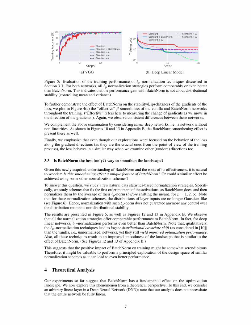
Figure 5: Evaluation of the training performance of `p normalization techniques discussed inSection 3.3. For both networks, all `p normalization strategies perform comparably or even betterthan BatchNorm. This indicates that the performance gain with BatchNorm is not about distributionalstability (controlling mean and variance).

To further demonstrate the effect of BatchNorm on the stability/Lipschitzness of the gradients of theloss, we plot in Figure 4(c) the “effective” β-smoothness of the vanilla and BatchNorm networksthroughout the training. (“Effective” refers here to measuring the change of gradients as we move inthe direction of the gradients.). Again, we observe consistent differences between these networks.

We complement the above examination by considering linear deep networks, i.e., a network withoutnon-linearities. As shown in Figures 10 and 13 in Appendix B, the BatchNorm smoothening effect ispresent there as well.

Finally, we emphasize that even though our explorations were focused on the behavior of the lossalong the gradient directions (as they are the crucial ones from the point of view of the trainingprocess), the loss behaves in a similar way when we examine other (random) directions too.

3.3 Is BatchNorm the best (only?) way to smoothen the landscape?

Given this newly acquired understanding of BatchNorm and the roots of its effectiveness, it is naturalto wonder: Is this smoothening effect a unique feature of BatchNorm? Or could a similar effect beachieved using some other normalization schemes?

To answer this question, we study a few natural data statistics-based normalization strategies. Specifi-cally, we study schemes that fix the first order moment of the activations, as BatchNorm does, and thennormalizes them by the average of their `p-norm (before shifting the mean), for p = 1, 2,∞. Notethat for these normalization schemes, the distributions of layer inputs are no longer Gaussian-like(see Figure 6). Hence, normalization with such `p-norm does not guarantee anymore any control overthe distribution moments nor distributional stability.

The results are presented in Figure 5, as well as Figures 12 and 13 in Appendix B. We observethat all the normalization strategies offer comparable performance to BatchNorm. In fact, for deeplinear networks, `1–normalization performs even better than BatchNorm. Note that, qualitatively,the `p–normalization techniques lead to larger distributional covariate shift (as considered in [10])than the vanilla, i.e., unnormalized, networks, yet they still yield improved optimization performance.Also, all these techniques result in an improved smoothness of the landscape that is similar to theeffect of BatchNorm. (See Figures 12 and 13 of Appendix B.)

This suggests that the positive impact of BatchNorm on training might be somewhat serendipitous.Therefore, it might be valuable to perform a principled exploration of the design space of similarnormalization schemes as it can lead to even better performance.

4 Theoretical Analysis

Our experiments so far suggest that BatchNorm has a fundamental effect on the optimizationlandscape. We now explore this phenomenon from a theoretical perspective. To this end, we consideran arbitrary linear layer in a Deep Neural Network (DNN); note that our analysis does not necessitatethat the entire network be fully linear.

7

Laye

r #11

Standard Standard + BatchNorm Standard + L1 Norm Standard + L2 Norm Standard + L Norm

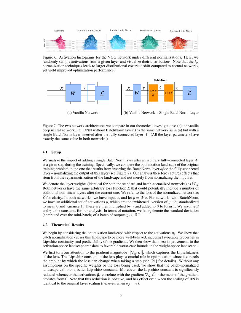
Figure 6: Activation histograms for the VGG network under different normalizations. Here, werandomly sample activations from a given layer and visualize their distributions. Note that the `p-normalization techniques leads to larger distributional covariate shift compared to normal networks,yet yield improved optimization performance.

yt − μσ

yyxγ y + β

zBatchNorm

W L

(a) Vanilla Network

yt − μσ

yyxγ y + β

zBatchNorm

W bL

(b) Vanilla Network + Single BatchNorm Layer

Figure 7: The two network architectures we compare in our theoretical investigations: (a) the vanilladeep neural network, i.e., DNN without BatchNorm layer; (b) the same network as in (a) but with asingle BatchNorm layer inserted after the fully-connected layer W . (All the layer parameters haveexactly the same value in both networks.)

4.1 Setup

We analyze the impact of adding a single BatchNorm layer after an arbitrary fully-connected layer Wat a given step during the training. Specifically, we compare the optimization landscape of the originaltraining problem to the one that results from inserting the BatchNorm layer after the fully-connectedlayer – normalizing the output of this layer (see Figure 7). Our analysis therefore captures effects thatstem from the reparametrization of the landscape and not merely from normalizing the inputs x.

We denote the layer weights (identical for both the standard and batch-normalized networks) as Wij .Both networks have the same arbitrary loss function L that could potentially include a number ofadditional non-linear layers after the current one. We refer to the loss of the normalized network asL for clarity. In both networks, we have input x, and let y = Wx. For networks with BatchNorm,we have an additional set of activations y, which are the “whitened” version of y, i.e. standardizedto mean 0 and variance 1. These are then multiplied by γ and added to β to form z. We assume βand γ to be constants for our analysis. In terms of notation, we let σj denote the standard deviation(computed over the mini-batch) of a batch of outputs yj ∈ Rm.

4.2 Theoretical Results

We begin by considering the optimization landscape with respect to the activations yj . We show thatbatch normalization causes this landscape to be more well-behaved, inducing favourable properties inLipschitz-continuity, and predictability of the gradients. We then show that these improvements in theactivation-space landscape translate to favorable worst-case bounds in the weight-space landscape.

We first turn our attention to the gradient magnitude∣∣∣∣∇yj

L∣∣∣∣, which captures the Lipschitzness

of the loss. The Lipschitz constant of the loss plays a crucial role in optimization, since it controlsthe amount by which the loss can change when taking a step (see [21] for details). Without anyassumptions on the specific weights or the loss being used, we show that the batch-normalizedlandscape exhibits a better Lipschitz constant. Moreover, the Lipschitz constant is significantlyreduced whenever the activations yj correlate with the gradient ∇yj L or the mean of the gradientdeviates from 0. Note that this reduction is additive, and has effect even when the scaling of BN isidentical to the original layer scaling (i.e. even when σj = γ).

8

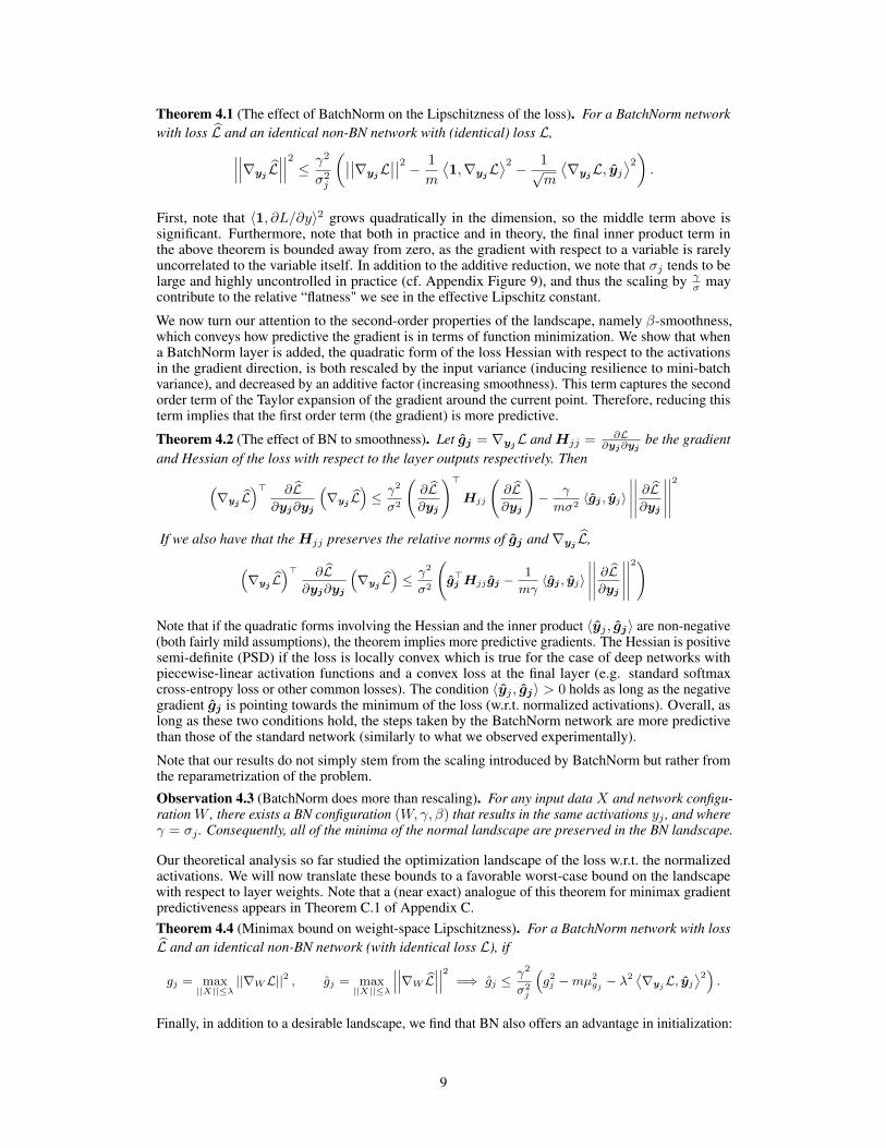
Theorem 4.1 (The effect of BatchNorm on the Lipschitzness of the loss). For a BatchNorm networkwith loss L and an identical non-BN network with (identical) loss L,

∣∣∣∣∣∣∇yj

L∣∣∣∣∣∣2

≤ γ2

σ2j

(∣∣∣∣∇yjL∣∣∣∣2 − 1

m

⟨1,∇yj

L⟩2 − 1√

m

⟨∇yjL, yj

⟩2).

First, note that 〈1, ∂L/∂y〉2 grows quadratically in the dimension, so the middle term above issignificant. Furthermore, note that both in practice and in theory, the final inner product term inthe above theorem is bounded away from zero, as the gradient with respect to a variable is rarelyuncorrelated to the variable itself. In addition to the additive reduction, we note that σj tends to belarge and highly uncontrolled in practice (cf. Appendix Figure 9), and thus the scaling by γ

σ maycontribute to the relative “flatness" we see in the effective Lipschitz constant.

We now turn our attention to the second-order properties of the landscape, namely β-smoothness,which conveys how predictive the gradient is in terms of function minimization. We show that whena BatchNorm layer is added, the quadratic form of the loss Hessian with respect to the activationsin the gradient direction, is both rescaled by the input variance (inducing resilience to mini-batchvariance), and decreased by an additive factor (increasing smoothness). This term captures the secondorder term of the Taylor expansion of the gradient around the current point. Therefore, reducing thisterm implies that the first order term (the gradient) is more predictive.

Theorem 4.2 (The effect of BN to smoothness). Let gj = ∇yjL andHjj =

∂L∂yj∂yj

be the gradientand Hessian of the loss with respect to the layer outputs respectively. Then

(∇yj L

)> ∂L∂yj∂yj

(∇yj L

)≤ γ2

σ2

(∂L∂yj

)>Hjj

(∂L∂yj

)− γ

mσ2〈gj , yj〉

∣∣∣∣∣∣∣∣∣∣ ∂L∂yj

∣∣∣∣∣∣∣∣∣∣2

If we also have that theHjj preserves the relative norms of gj and ∇yjL,

(∇yj L

)> ∂L∂yj∂yj

(∇yj L

)≤ γ2

σ2

(g>j Hjj gj −

1

mγ〈gj , yj〉

∣∣∣∣∣∣∣∣∣∣ ∂L∂yj

∣∣∣∣∣∣∣∣∣∣2)

Note that if the quadratic forms involving the Hessian and the inner product 〈yj , gj〉 are non-negative(both fairly mild assumptions), the theorem implies more predictive gradients. The Hessian is positivesemi-definite (PSD) if the loss is locally convex which is true for the case of deep networks withpiecewise-linear activation functions and a convex loss at the final layer (e.g. standard softmaxcross-entropy loss or other common losses). The condition 〈yj , gj〉 > 0 holds as long as the negativegradient gj is pointing towards the minimum of the loss (w.r.t. normalized activations). Overall, aslong as these two conditions hold, the steps taken by the BatchNorm network are more predictivethan those of the standard network (similarly to what we observed experimentally).

Note that our results do not simply stem from the scaling introduced by BatchNorm but rather fromthe reparametrization of the problem.

Observation 4.3 (BatchNorm does more than rescaling). For any input data X and network configu-ration W , there exists a BN configuration (W,γ, β) that results in the same activations yj , and whereγ = σj . Consequently, all of the minima of the normal landscape are preserved in the BN landscape.

Our theoretical analysis so far studied the optimization landscape of the loss w.r.t. the normalizedactivations. We will now translate these bounds to a favorable worst-case bound on the landscapewith respect to layer weights. Note that a (near exact) analogue of this theorem for minimax gradientpredictiveness appears in Theorem C.1 of Appendix C.Theorem 4.4 (Minimax bound on weight-space Lipschitzness). For a BatchNorm network with lossL and an identical non-BN network (with identical loss L), if

gj = max||X||≤λ

||∇WL||2 , gj = max||X||≤λ

∣∣∣∣∣∣∇W L∣∣∣∣∣∣2 =⇒ gj ≤γ2

σ2j

(g2j −mµ2

gj − λ2 ⟨∇yjL, yj

⟩2).

Finally, in addition to a desirable landscape, we find that BN also offers an advantage in initialization:

9

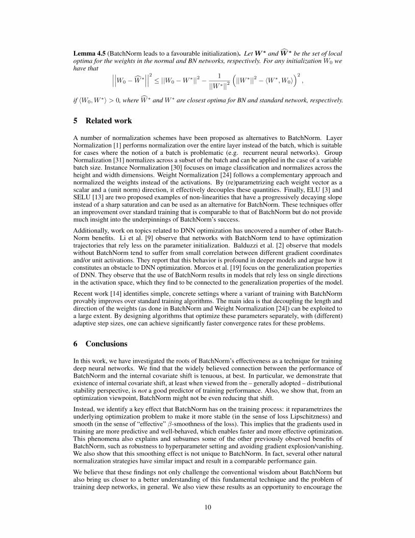
Lemma 4.5 (BatchNorm leads to a favourable initialization). LetW ∗ and W ∗ be the set of localoptima for the weights in the normal and BN networks, respectively. For any initialization W0 wehave that ∣∣∣

∣∣∣W0 − W ∗∣∣∣∣∣∣2

≤ ||W0 −W ∗||2 −1

||W ∗||2(||W ∗||2 − 〈W ∗,W0〉

)2,

if 〈W0,W∗〉 > 0, where W ∗ and W ∗ are closest optima for BN and standard network, respectively.

5 Related work

A number of normalization schemes have been proposed as alternatives to BatchNorm. LayerNormalization [1] performs normalization over the entire layer instead of the batch, which is suitablefor cases where the notion of a batch is problematic (e.g. recurrent neural networks). GroupNormalization [31] normalizes across a subset of the batch and can be applied in the case of a variablebatch size. Instance Normalization [30] focuses on image classification and normalizes across theheight and width dimensions. Weight Normalization [24] follows a complementary approach andnormalized the weights instead of the activations. By (re)parametrizing each weight vector as ascalar and a (unit norm) direction, it effectively decouples these quantities. Finally, ELU [3] andSELU [13] are two proposed examples of non-linearities that have a progressively decaying slopeinstead of a sharp saturation and can be used as an alternative for BatchNorm. These techniques offeran improvement over standard training that is comparable to that of BatchNorm but do not providemuch insight into the underpinnings of BatchNorm’s success.

Additionally, work on topics related to DNN optimization has uncovered a number of other Batch-Norm benefits. Li et al. [9] observe that networks with BatchNorm tend to have optimizationtrajectories that rely less on the parameter initialization. Balduzzi et al. [2] observe that modelswithout BatchNorm tend to suffer from small correlation between different gradient coordinatesand/or unit activations. They report that this behavior is profound in deeper models and argue how itconstitutes an obstacle to DNN optimization. Morcos et al. [19] focus on the generalization propertiesof DNN. They observe that the use of BatchNorm results in models that rely less on single directionsin the activation space, which they find to be connected to the generalization properties of the model.

Recent work [14] identifies simple, concrete settings where a variant of training with BatchNormprovably improves over standard training algorithms. The main idea is that decoupling the length anddirection of the weights (as done in BatchNorm and Weight Normalization [24]) can be exploited toa large extent. By designing algorithms that optimize these parameters separately, with (different)adaptive step sizes, one can achieve significantly faster convergence rates for these problems.

6 Conclusions

In this work, we have investigated the roots of BatchNorm’s effectiveness as a technique for trainingdeep neural networks. We find that the widely believed connection between the performance ofBatchNorm and the internal covariate shift is tenuous, at best. In particular, we demonstrate thatexistence of internal covariate shift, at least when viewed from the – generally adopted – distributionalstability perspective, is not a good predictor of training performance. Also, we show that, from anoptimization viewpoint, BatchNorm might not be even reducing that shift.

Instead, we identify a key effect that BatchNorm has on the training process: it reparametrizes theunderlying optimization problem to make it more stable (in the sense of loss Lipschitzness) andsmooth (in the sense of “effective” β-smoothness of the loss). This implies that the gradients used intraining are more predictive and well-behaved, which enables faster and more effective optimization.This phenomena also explains and subsumes some of the other previously observed benefits ofBatchNorm, such as robustness to hyperparameter setting and avoiding gradient explosion/vanishing.We also show that this smoothing effect is not unique to BatchNorm. In fact, several other naturalnormalization strategies have similar impact and result in a comparable performance gain.

We believe that these findings not only challenge the conventional wisdom about BatchNorm butalso bring us closer to a better understanding of this fundamental technique and the problem oftraining deep networks, in general. We also view these results as an opportunity to encourage the

10

community to pursue a more systematic investigation of the algorithmic toolkit of deep learning andthe underpinnings of its effectiveness.

Finally, our focus here was on the impact of BatchNorm on training but our findings might also shedsome light on the BatchNorm’s tendency to improve generalization. Specifically, it could be the casethat the smoothening effect of BatchNorm’s reparametrization encourages the training process toconverge to more flat minima. Such minima are believed to facilitate better generalization [8, 11].We hope that future work will investigate this intriguing possibility.

Acknowledgements

We thank Ali Rahimi and Ben Recht for helpful comments on a preliminary version of this paper.

Shibani Santurkar was supported by the National Science Foundation (NSF) under grants IIS-1447786,IIS-1607189, and CCF-1563880, and the Intel Corporation. Dimitris Tsipras was supported in part bythe NSF grant CCF-1553428 and the NSF Frontier grant CNS-1413920. Andrew Ilyas was supportedin part by NSF awards CCF-1617730 and IIS-1741137, a Simons Investigator Award, a GoogleFaculty Research Award, and an MIT-IBM Watson AI Lab research grant. Aleksander Madry wassupported in part by an Alfred P. Sloan Research Fellowship, a Google Research Award, and the NSFgrants CCF-1553428 and CNS-1815221.

References[1] Jimmy Lei Ba, Jamie Ryan Kiros, and Geoffrey E Hinton. Layer normalization. arXiv preprint

arXiv:1607.06450, 2016.

[2] David Balduzzi, Marcus Frean, Lennox Leary, JP Lewis, Kurt Wan-Duo Ma, and Brian McWilliams.The shattered gradients problem: If resnets are the answer, then what is the question? arXiv preprintarXiv:1702.08591, 2017.

[3] Djork-Arné Clevert, Thomas Unterthiner, and Sepp Hochreiter. Fast and accurate deep network learningby exponential linear units (elus). arXiv preprint arXiv:1511.07289, 2015.

[4] Xavier Glorot and Yoshua Bengio. Understanding the difficulty of training deep feedforward neuralnetworks. In Proceedings of the thirteenth international conference on artificial intelligence and statistics,pages 249–256, 2010.

[5] Alex Graves, Abdel-rahman Mohamed, and Geoffrey Hinton. Speech recognition with deep recurrentneural networks. In Acoustics, speech and signal processing (icassp), 2013 ieee international conferenceon, pages 6645–6649. IEEE, 2013.

[6] Moritz Hardt and Tengyu Ma. Identity matters in deep learning. arXiv preprint arXiv:1611.04231, 2016.

[7] Kaiming He, Xiangyu Zhang, Shaoqing Ren, and Jian Sun. Deep residual learning for image recognition.In Proceedings of the IEEE Conference on Computer Vision and Pattern Recognition, 2016.

[8] Sepp Hochreiter and Jürgen Schmidhuber. Flat minima. Neural Computation, 9(1):1–42, 1997.

[9] Daniel Jiwoong Im, Michael Tao, and Kristin Branson. An empirical analysis of deep network loss surfaces.arXiv preprint arXiv:1612.04010, 2016.

[10] Sergey Ioffe and Christian Szegedy. Batch normalization: Accelerating deep network training by reducinginternal covariate shift. arXiv preprint arXiv:1502.03167, 2015.

[11] Nitish Shirish Keskar, Dheevatsa Mudigere, Jorge Nocedal, Mikhail Smelyanskiy, and Ping Tak PeterTang. On large-batch training for deep learning: Generalization gap and sharp minima. arXiv preprintarXiv:1609.04836, 2016.

[12] Diederik P Kingma and Jimmy Ba. Adam: A method for stochastic optimization. arXiv preprintarXiv:1412.6980, 2014.

[13] Günter Klambauer, Thomas Unterthiner, Andreas Mayr, and Sepp Hochreiter. Self-normalizing neuralnetworks. In Advances in Neural Information Processing Systems, pages 972–981, 2017.

[14] Jonas Kohler, Hadi Daneshmand, Aurelien Lucchi, Ming Zhou, Klaus Neymeyr, and Thomas Hofmann.Towards a theoretical understanding of batch normalization. arXiv preprint arXiv:1805.10694, 2018.

[15] Alex Krizhevsky and Geoffrey Hinton. Learning multiple layers of features from tiny images. 2009.

[16] Alex Krizhevsky, Ilya Sutskever, and Geoffrey E Hinton. Imagenet classification with deep convolutionalneural networks. In Advances in neural information processing systems, pages 1097–1105, 2012.

[17] Hao Li, Zheng Xu, Gavin Taylor, and Tom Goldstein. Visualizing the loss landscape of neural nets. arXivpreprint arXiv:1712.09913, 2017.

11

[18] Volodymyr Mnih, Koray Kavukcuoglu, David Silver, Andrei A Rusu, Joel Veness, Marc G Bellemare,Alex Graves, Martin Riedmiller, Andreas K Fidjeland, Georg Ostrovski, et al. Human-level control throughdeep reinforcement learning. Nature, 518(7540):529, 2015.

[19] Ari S Morcos, David GT Barrett, Neil C Rabinowitz, and Matthew Botvinick. On the importance of singledirections for generalization. arXiv preprint arXiv:1803.06959, 2018.

[20] Vinod Nair and Geoffrey E Hinton. Rectified linear units improve restricted boltzmann machines. InProceedings of the 27th international conference on machine learning (ICML-10), 2010.

[21] Yurii Nesterov. Introductory lectures on convex optimization: A basic course, volume 87. Springer Science& Business Media, 2013.

[22] Ali Rahimi and Ben Recht. Back when we were kids. In NIPS Test-of-Time Award Talk, 2017.

[23] Olga Russakovsky, Jia Deng, Hao Su, Jonathan Krause, Sanjeev Satheesh, Sean Ma, Zhiheng Huang,Andrej Karpathy, Aditya Khosla, Michael Bernstein, Alexander C. Berg, and Li Fei-Fei. ImageNet LargeScale Visual Recognition Challenge. International Journal of Computer Vision (IJCV), 115(3), 2015.

[24] Tim Salimans and Diederik P Kingma. Weight normalization: A simple reparameterization to acceleratetraining of deep neural networks. In Advances in Neural Information Processing Systems, 2016.

[25] David Silver, Aja Huang, Chris J Maddison, Arthur Guez, Laurent Sifre, George Van Den Driessche, JulianSchrittwieser, Ioannis Antonoglou, Veda Panneershelvam, Marc Lanctot, et al. Mastering the game of gowith deep neural networks and tree search. nature, 529(7587):484–489, 2016.

[26] Karen Simonyan and Andrew Zisserman. Very deep convolutional networks for large-scale image recogni-tion. arXiv preprint arXiv:1409.1556, 2014.

[27] Nitish Srivastava, Geoffrey Hinton, Alex Krizhevsky, Ilya Sutskever, and Ruslan Salakhutdinov. Dropout:A simple way to prevent neural networks from overfitting. The Journal of Machine Learning Research,15(1), 2014.

[28] Ilya Sutskever, James Martens, George Dahl, and Geoffrey Hinton. On the importance of initialization andmomentum in deep learning. In International conference on machine learning, 2013.

[29] Ilya Sutskever, Oriol Vinyals, and Quoc V Le. Sequence to sequence learning with neural networks. InAdvances in neural information processing systems, pages 3104–3112, 2014.

[30] Dmitry Ulyanov, Andrea Vedaldi, and Victor Lempitsky. Instance normalization: The missing ingredientfor fast stylization. arXiv preprint arXiv:1607.08022, 2016.

[31] Yuxin Wu and Kaiming He. Group normalization. arXiv preprint arXiv:1803.08494, 2018.

12

A Experimental Setup

In Section A.1, we provide details regarding the architectures used in our analysis. Then in Section A.2we discuss the specifics of the setup and measurements used in our experiments.

A.1 Models

We use two standard deep architectures – a VGG-like network, and a deep linear network (DLN). TheVGG model achieves close to state-of-the-art performance while being fairly simple4. Preliminaryexperiments on other architectures gave similar results. We study DLNs with full-batch trainingsince they allow us to isolate the effect of non-linearities, as well as the stochasticity of the trainingprocedure. Both these architectures show clear a performance benefits with BatchNorm.

Specific details regarding both architectures are provided below:

1. Convolutional VGG architecture on CIFAR10 (VGG):We fit a VGG-like network, a standard convolutional architecture [26], to a canonical imageclassification problem (CIFAR10 [15]). We optimize using standard stochastic gradientdescent and train for 15, 000 steps (training accuracy plateaus). We use a batch size of 128and a fixed learning rate of 0.1 unless otherwise specified. Moreover, since our focus is ontraining, we do not use data augmentation. This architecture can fit the training dataset welland achieves close to state-of-the art test performance. Our network achieves a test accuracyof 83% with BatchNorm and 80% without (this becomes 92% and 88% respectively withdata augmentation).

2. 25-Layer Deep Linear Network on Synthetic Gaussian Data (DLN):DLN are a factorized approach to solving a simple regression problem, i.e., fitting Ax fromx. Specifically, we consider a deep network with k fully connected layers and an `2 loss.Thus, we are minimizing ‖W1 . . .Wkx − Ax‖22 over Wi

5. We generate inputs x from aGaussian Distribution and a matrix A with i.i.d. Gaussian entries. We choose k to be 25,and the dimensions of A to be 10× 10. All the matrices Wi are square and have the samedimensions. We train DLN using full-batch gradient descent for 10, 000 steps (training lossplateaus).The size of the dataset is 1000 (same as the batch size) and the learning rate is10−6 unless otherwise specified.

For both networks we use standard Glorot initialization [4]. Further the learning rates were selectedbased on hyperparameter optimization to find a configuration where the training performance for thenetwork was the best.

A.2 Details

A.2.1 “Noisy” BatchNorm Layers

Consider ai,j , the j-th activation of the i-th example in the batch. Note that batch norm will ensurethat the distribution of a·,j for some j will have fixed mean and variance (possibly learnable).

At every time step, our noise model consists of perturbing each activation for each sample in a batchwith noise i.i.d. from a non-zero mean, non-unit variance distribution Dt

j . The distributionDtj itself is

time varying and its parameters are drawn i.i.d from another distributionDj . The specific noise modelis described in Algorithm 1. In our experiments, nµ = 0.5, nσ = 1.25 and rµ = rσ = 0.1. (Forconvolutional layers, we follow the standard convention of treating the height and width dimensionsas part of the batch.)

4We choose to not experiment with ResNets [7] since they seem to provide several similar benefits toBatchNorm [6] and would introduce conflating factors into our study.

5While the factorized formulation is equivalent to a single matrix in terms of expressivity, the optimizationlandscape is drastically different [6].

13

Algorithm 1 “Noisy” BatchNorm

1: % For constants nm, nv , rm, rv .2:3: for each layer at time t do4: ati,j ← Batch-normalized activation for unit j and sample i5:6: for each j do . Sample the parameters (mt

j , vtj) of Dt

j from Dj

7: µt ∼ U(−nµ, nµ)8: σt ∼ U(1, nσ)

9:10: for each i do . Sample noise from Dt

j11: for each j do12: mt

i,j ∼ U(µ− rµ, µ+ rµ)

13: sti,j ∼ N (σ, rσ)

14: ati,j ← sti,j · ai,j +mti,j

While plotting the distribution of activations, we sample random activations from any given layer ofthe network and plot its distribution over the batch dimension for fully connected layers, and over thebatch, height, width dimension for convolutional layers as is standard convention in BatchNorm forconvolutional networks.

A.2.2 Loss Landscape

To measure the smoothness of the loss landscape of a network during the course of training, weessentially take steps of different lengths in the direction of the gradient and measure the loss valuesobtained at each step. Note that this is not a training procedure, but an evaluation of the local losslandscape at every step of the training process.

For VGG we consider steps of length ranging from [1/2, 4]× step size, whereas for DLN we choose[1/100, 30]× step size. Here step size denotes the hyperparameter setting with which the network isbeing trained. We choose these ranges to roughly reflect the range of parameters that are valid forstandard training of these models. The VGG network is much more sensitive to the learning ratechoices (probably due to the non-linearities it includes), so we perform line search over a restrictedrange of parameters. Further, the maximum step size was chosen slightly smaller than the learningrate at which the standard (no BatchNorm) network diverges during training.

B Omitted Figures

Additional visualizations for the analysis performed in Section 3.1 are presented below.

14

0

1

Laye

r#: 2

| t + 1 t|

0

1

Laye

r#: 2

| 2t + 1

2t |


0

1

Laye

r#: 9

0

1

Laye

r#: 9

0 5k 10k 15kSteps

0

1

Laye

r#: 1

3

0 5k 10k 15kSteps

0

1

Laye

r#: 1

3

(a)

0.50

0.25

0.00

0.25

Laye

r#: 2

t 0

0.4

0.2

0.0

0.2

Laye

r#: 2

2t

20


0.0

0.5

1.0

Laye

r#: 9

0.4

0.2

0.0

0.2

Laye

r#: 9

0 5k 10k 15kSteps

0.25

0.00

0.25

0.50

0.75

Laye

r#: 1

3

0 5k 10k 15kSteps

0.0

0.5

1.0

Laye

r#: 1

3

(b)

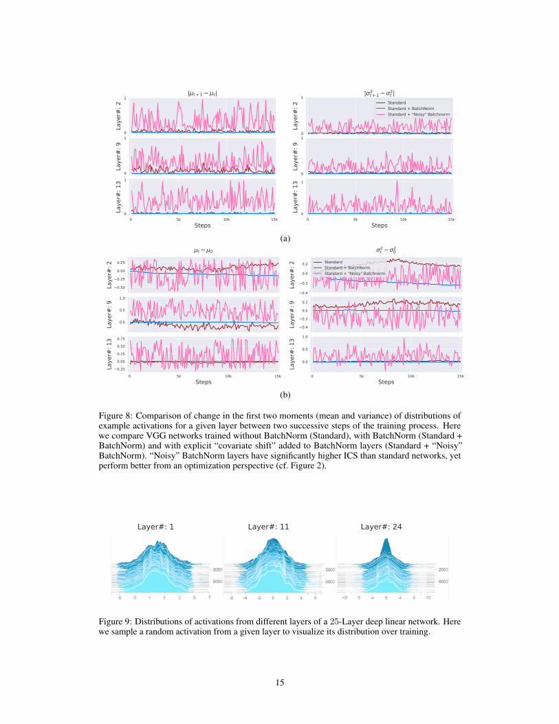
Figure 8: Comparison of change in the first two moments (mean and variance) of distributions ofexample activations for a given layer between two successive steps of the training process. Herewe compare VGG networks trained without BatchNorm (Standard), with BatchNorm (Standard +BatchNorm) and with explicit “covariate shift” added to BatchNorm layers (Standard + “Noisy”BatchNorm). “Noisy” BatchNorm layers have significantly higher ICS than standard networks, yetperform better from an optimization perspective (cf. Figure 2).

Layer#: 1 Layer#: 11 Layer#: 24

Figure 9: Distributions of activations from different layers of a 25-Layer deep linear network. Herewe sample a random activation from a given layer to visualize its distribution over training.

15

0 5k 10kSteps

104

106

108

1010

1012

1014

Loss

Lan

dsca

pe


(a) loss landscape

0 5k 10kSteps

102

104

106

108

1010

1012

1014

1016

Grad

ient

Pre

dict

iven

ess Standard


(b) gradient predictiveness

0 5k 10kSteps

107

109

1011

1013

1015

-sm

ooth

ness


(c) “effective” β-smoothness

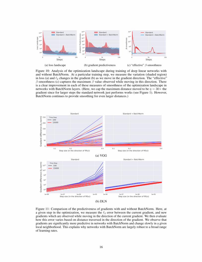
Figure 10: Analysis of the optimization landscape during training of deep linear networks withand without BatchNorm. At a particular training step, we measure the variation (shaded region)in loss (a) and `2 changes in the gradient (b) as we move in the gradient direction. The “effective”β-smoothness (c) captures the maximum β value observed while moving in this direction. Thereis a clear improvement in each of these measures of smoothness of the optimization landscape innetworks with BatchNorm layers. (Here, we cap the maximum distance moved to be η = 30× thegradient since for larger steps the standard network just performs works (see Figure 1). However,BatchNorm continues to provide smoothing for even larger distances.)

0.1 0.2 0.4Step size (in the direction of f(x))

0

50

100

150

200

250

Grad

ient

diff

eren

ce (

2-nor

m)

StandardTime Step

10015000

0.1 0.2 0.4Step size (in the direction of f(x))


(a) VGG

1e-08 1e-07 1e-06 1e-05Step size (in the direction of f(x))

103

105

107

109

1011

1013

Grad

ient

diff

eren

ce (

2-nor

m)

StandardTime Step

10015000

1e-08 1e-07 1e-06 1e-05Step size (in the direction of f(x))


(b) DLN

Figure 11: Comparison of the predictiveness of gradients with and without BatchNorm. Here, ata given step in the optimization, we measure the `2 error between the current gradient, and newgradients which are observed while moving in the direction of the current gradient. We then evaluatehow this error varies based on distance traversed in the direction of the gradient. We observe thatgradients are significantly more predictive in networks with BatchNorm and change slowly in a givenlocal neighborhood. This explains why networks with BatchNorm are largely robust to a broad rangeof learning rates.

16

0 5k 10k 15kSteps

20

40

60

80

100

Trai

ning

Acc

urac

y (%

)

(a)



0 5k 10k 15kSteps

100

101

Loss

Lan

dsca

pe

(b)

StandardStandard + BatchnormStandard + L1


0 5k 10k 15kSteps

0

200

400

Grad

ient

Pre

dict

iven

ess

(c)



0 5k 10k 15kSteps

5

10

15

20

25

30

35

40

45

-sm

ooth

ness

(d)



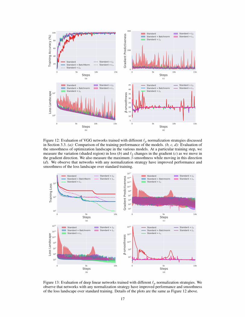
Figure 12: Evaluation of VGG networks trained with different `p normalization strategies discussedin Section 3.3. (a): Comparison of the training performance of the models. (b, c, d): Evaluation ofthe smoothness of optimization landscape in the various models. At a particular training step, wemeasure the variation (shaded region) in loss (b) and `2 changes in the gradient (c) as we move inthe gradient direction. We also measure the maximum β-smoothness while moving in this direction(d). We observe that networks with any normalization strategy have improved performance andsmoothness of the loss landscape over standard training.

0 5k 10kSteps

102

103

104

Trai

ning

Los

s

(a)



0 5k 10kSteps

103

105

107

109

1011

1013

1015

Loss

Lan

dsca

pe

(b)



0 5k 10kSteps

101

103

105

107

109

1011

1013

1015

1017

Grad

ient

Pre

dict

iven

ess

(c)



0 5k 10kSteps

107

109

1011

1013

1015

-sm

ooth

ness

(d)



Figure 13: Evaluation of deep linear networks trained with different `p normalization strategies. Weobserve that networks with any normalization strategy have improved performance and smoothnessof the loss landscape over standard training. Details of the plots are the same as Figure 12 above.

17

C Proofs

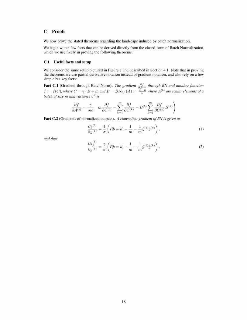
We now prove the stated theorems regarding the landscape induced by batch normalization.

We begin with a few facts that can be derived directly from the closed-form of Batch Normalization,which we use freely in proving the following theorems.

C.1 Useful facts and setup

We consider the same setup pictured in Figure 7 and described in Section 4.1. Note that in provingthe theorems we use partial derivative notation instead of gradient notation, and also rely on a fewsimple but key facts:

Fact C.1 (Gradient through BatchNorm). The gradient ∂f∂A(b) through BN and another function

f := f(C), where C = γ ·B + β, and B = BN0,1(A) :=A−µσ where A(b) are scalar elements of a

batch of size m and variance σ2 is

∂f

∂A(b)=

γ

mσ

(m

∂f

∂C(b)−

m∑

k=1

∂f

∂C(k)−B(b)

m∑

k=1

∂f

∂C(k)B(k)

)

Fact C.2 (Gradients of normalized outputs). A convenient gradient of BN is given as

∂y(b)

∂y(k)=

1

σ

(1[b = k]− 1

m− 1

my(b)y(k)

), (1)

and thus∂z

(b)j

∂y(k)=γ

σ

(1[b = k]− 1

m− 1

my(b)y(k)

), (2)

18

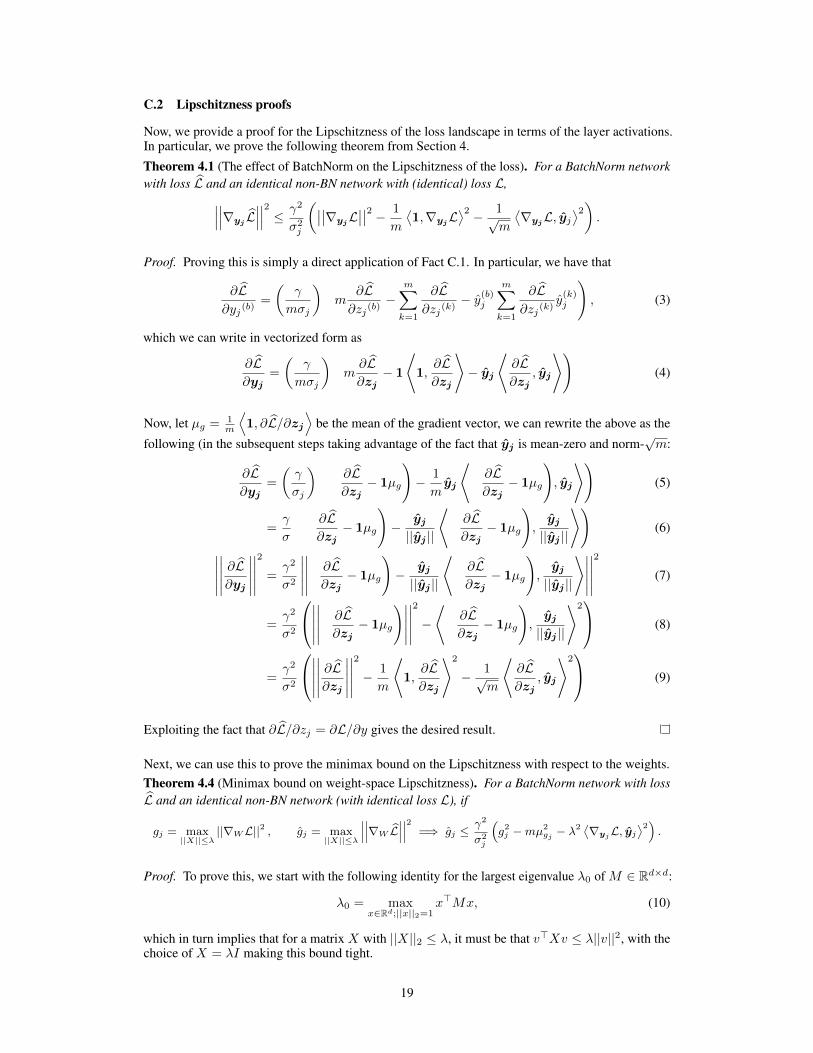
C.2 Lipschitzness proofs

Now, we provide a proof for the Lipschitzness of the loss landscape in terms of the layer activations.In particular, we prove the following theorem from Section 4.

Theorem 4.1 (The effect of BatchNorm on the Lipschitzness of the loss). For a BatchNorm networkwith loss L and an identical non-BN network with (identical) loss L,

∣∣∣∣∣∣∇yj

L∣∣∣∣∣∣2

≤ γ2

σ2j

(∣∣∣∣∇yjL∣∣∣∣2 − 1

m

⟨1,∇yj

L⟩2 − 1√

m

⟨∇yjL, yj

⟩2).

Proof. Proving this is simply a direct application of Fact C.1. In particular, we have that

∂L∂yj(b)

=

(γ

mσj

)(m

∂L∂zj(b)

−m∑

k=1

∂L∂zj(k)

− y(b)jm∑

k=1

∂L∂zj(k)

y(k)j

), (3)

which we can write in vectorized form as

∂L∂yj

=

(γ

mσj

)(m∂L∂zj− 1

⟨1,∂L∂zj

⟩− yj

⟨∂L∂zj

, yj

⟩)(4)

Now, let µg = 1m

⟨1, ∂L/∂zj

⟩be the mean of the gradient vector, we can rewrite the above as the

following (in the subsequent steps taking advantage of the fact that yj is mean-zero and norm-√m:

∂L∂yj

=

(γ

σj

)((∂L∂zj− 1µg

)− 1

myj

⟨(∂L∂zj− 1µg

), yj

⟩)(5)

=γ

σ

((∂L∂zj− 1µg

)− yj||yj ||


),yj||yj ||

⟩)(6)

∣∣∣∣∣

∣∣∣∣∣∂L∂yj

∣∣∣∣∣

∣∣∣∣∣

2

=γ2

σ2

∣∣∣∣∣

∣∣∣∣∣

(∂L∂zj− 1µg

)− yj||yj ||


),yj||yj ||

⟩∣∣∣∣∣

∣∣∣∣∣

2

(7)

=γ2

σ2

∣∣∣∣∣

∣∣∣∣∣

(∂L∂zj− 1µg

)∣∣∣∣∣

∣∣∣∣∣

2

−⟨(

∂L∂zj− 1µg

),yj||yj ||

⟩2 (8)

=γ2

σ2

∣∣∣∣∣

∣∣∣∣∣∂L∂zj

∣∣∣∣∣

∣∣∣∣∣

2

− 1

m

⟨1,∂L∂zj

⟩2

− 1√m

⟨∂L∂zj

, yj

⟩2 (9)

Exploiting the fact that ∂L/∂zj = ∂L/∂y gives the desired result.

Next, we can use this to prove the minimax bound on the Lipschitzness with respect to the weights.Theorem 4.4 (Minimax bound on weight-space Lipschitzness). For a BatchNorm network with lossL and an identical non-BN network (with identical loss L), if

gj = max||X||≤λ

||∇WL||2 , gj = max||X||≤λ

∣∣∣∣∣∣∇W L∣∣∣∣∣∣2 =⇒ gj ≤γ2

σ2j

(g2j −mµ2

gj − λ2 ⟨∇yjL, yj

⟩2).

Proof. To prove this, we start with the following identity for the largest eigenvalue λ0 of M ∈ Rd×d:

λ0 = maxx∈Rd;||x||2=1

x>Mx, (10)

which in turn implies that for a matrix X with ||X||2 ≤ λ, it must be that v>Xv ≤ λ||v||2, with thechoice of X = λI making this bound tight.

19

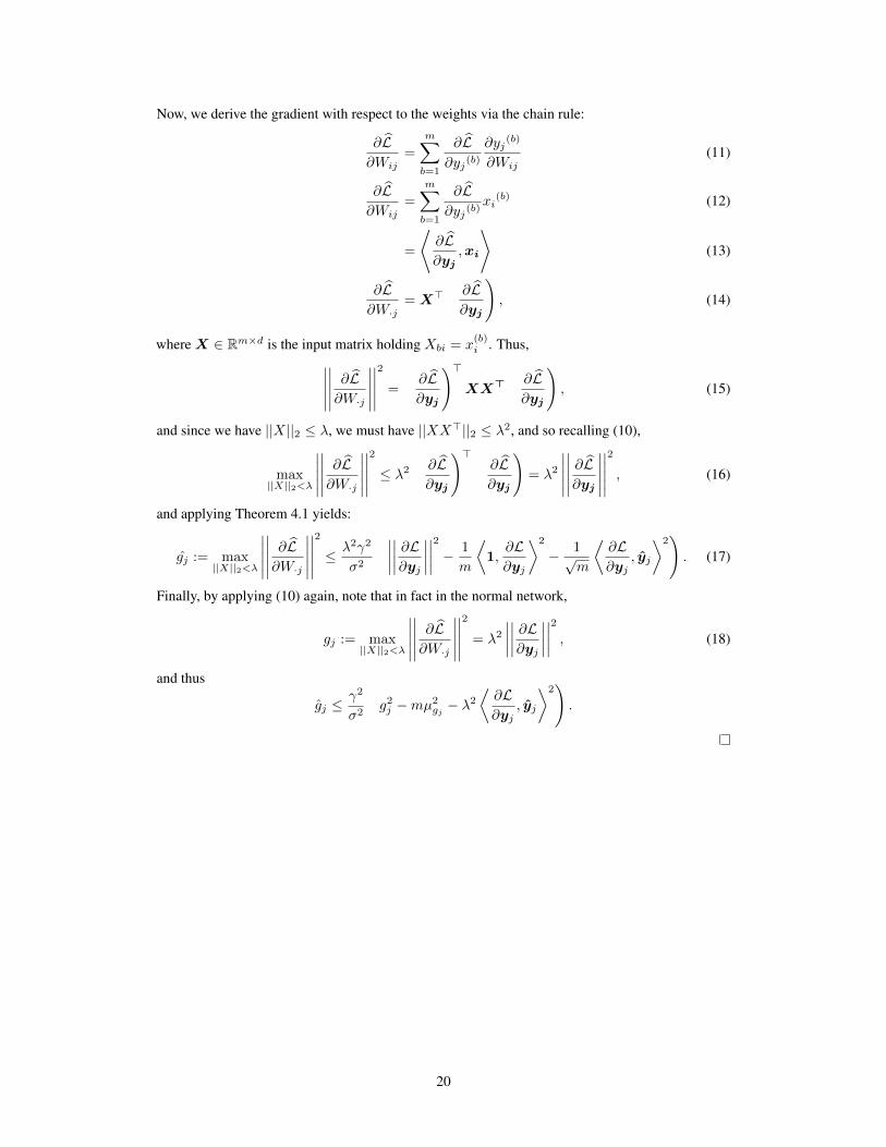
Now, we derive the gradient with respect to the weights via the chain rule:

∂L∂Wij

=

m∑

b=1

∂L∂yj(b)

∂yj(b)

∂Wij(11)

∂L∂Wij

=

m∑

b=1

∂L∂yj(b)

xi(b) (12)

=

⟨∂L∂yj

,xi

⟩(13)

∂L∂W·j

=X>

(∂L∂yj

), (14)

whereX ∈ Rm×d is the input matrix holding Xbi = x(b)i . Thus,

∣∣∣∣∣

∣∣∣∣∣∂L∂W·j

∣∣∣∣∣

∣∣∣∣∣

2

=

(∂L∂yj

)>XX>

(∂L∂yj

), (15)

and since we have ||X||2 ≤ λ, we must have ||XX>||2 ≤ λ2, and so recalling (10),

max||X||2<λ

∣∣∣∣∣

∣∣∣∣∣∂L∂W·j

∣∣∣∣∣

∣∣∣∣∣

2

≤ λ2(∂L∂yj

)>(∂L∂yj

)= λ2

∣∣∣∣∣

∣∣∣∣∣∂L∂yj

∣∣∣∣∣

∣∣∣∣∣

2

, (16)

and applying Theorem 4.1 yields:

gj := max||X||2<λ

∣∣∣∣∣

∣∣∣∣∣∂L∂W·j

∣∣∣∣∣

∣∣∣∣∣

2

≤ λ2γ2

σ2

(∣∣∣∣∣∣∣∣∂L∂yj

∣∣∣∣∣∣∣∣2

− 1

m

⟨1,∂L∂yj

⟩2

− 1√m

⟨∂L∂yj

, yj

⟩2). (17)

Finally, by applying (10) again, note that in fact in the normal network,

gj := max||X||2<λ

∣∣∣∣∣

∣∣∣∣∣∂L∂W·j

∣∣∣∣∣

∣∣∣∣∣

2

= λ2∣∣∣∣∣∣∣∣∂L∂yj

∣∣∣∣∣∣∣∣2

, (18)

and thus

gj ≤γ2

σ2

(g2j −mµ2

gj − λ2⟨∂L∂yj

, yj

⟩2).

20

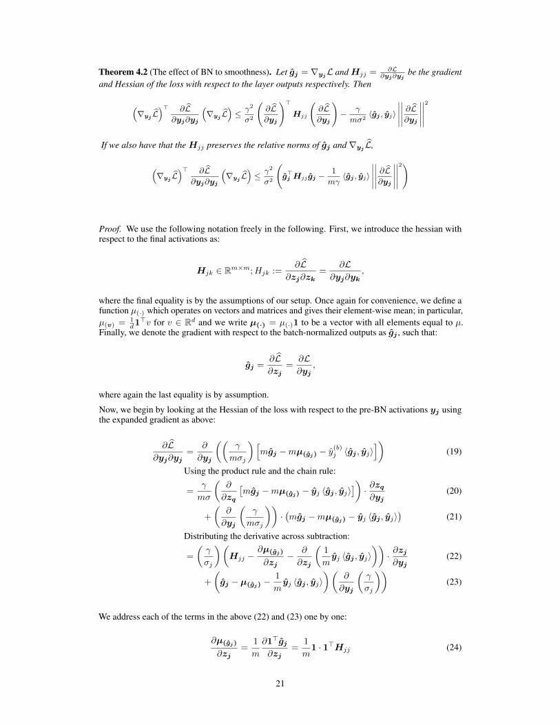
Theorem 4.2 (The effect of BN to smoothness). Let gj = ∇yjL andHjj =

∂L∂yj∂yj

be the gradientand Hessian of the loss with respect to the layer outputs respectively. Then

(∇yj L

)> ∂L∂yj∂yj

(∇yj L

)≤ γ2

σ2

(∂L∂yj

)>Hjj

(∂L∂yj

)− γ

mσ2〈gj , yj〉

∣∣∣∣∣∣∣∣∣∣ ∂L∂yj

∣∣∣∣∣∣∣∣∣∣2

If we also have that theHjj preserves the relative norms of gj and ∇yjL,

(∇yj L

)> ∂L∂yj∂yj

(∇yj L

)≤ γ2

σ2

(g>j Hjj gj −

1

mγ〈gj , yj〉

∣∣∣∣∣∣∣∣∣∣ ∂L∂yj

∣∣∣∣∣∣∣∣∣∣2)

Proof. We use the following notation freely in the following. First, we introduce the hessian withrespect to the final activations as:

Hjk ∈ Rm×m;Hjk :=∂L

∂zj∂zk=

∂L∂yj∂yk

,

where the final equality is by the assumptions of our setup. Once again for convenience, we define afunction µ(·) which operates on vectors and matrices and gives their element-wise mean; in particular,µ(v) = 1

d1>v for v ∈ Rd and we write µ(·) = µ(·)1 to be a vector with all elements equal to µ.

Finally, we denote the gradient with respect to the batch-normalized outputs as gj , such that:

gj =∂L∂zj

=∂L∂yj

,

where again the last equality is by assumption.

Now, we begin by looking at the Hessian of the loss with respect to the pre-BN activations yj usingthe expanded gradient as above:

∂L∂yj∂yj

=∂

∂yj

((γ

mσj

)[mgj −mµ(gj) − y

(b)j 〈gj , yj〉

])(19)

Using the product rule and the chain rule:

=γ

mσ

(∂

∂zq

[mgj −mµ(gj) − yj 〈gj , yj〉

])· ∂zq∂yj

(20)

+

(∂

∂yj

(γ

mσj

))·(mgj −mµ(gj) − yj 〈gj , yj〉

)(21)

Distributing the derivative across subtraction:

=

(γ

σj

)(Hjj −

∂µ(gj)

∂zj− ∂

∂zj

(1

myj 〈gj , yj〉

))· ∂zj∂yj

(22)

+

(gj − µ(gj) −

1

myj 〈gj , yj〉

)(∂

∂yj

(γ

σj

))(23)

We address each of the terms in the above (22) and (23) one by one:

∂µ(gj)

∂zj=

1

m

∂1>gj∂zj

=1

m1 · 1>Hjj (24)

21

∂

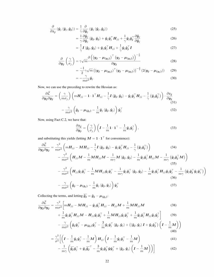
∂zj(yj 〈yj , gj〉) =

1

γ

∂

∂yj(yj 〈yj , gj〉) (25)

=1

γ

∂yj∂yj〈gj , yj〉+ yj y>j Hjj +

1

γyj g>j

∂yj∂yj

(26)

=1

γI 〈gj , yj〉+ yj y>j Hjj +

1

γyj g>j I (27)

∂

∂yj

(γ

σj

)= γ√m∂((yj − µ(yj)

)> (yj − µ(yj)

))− 12

∂yj(28)

=−12γ√m((yj − µ(yj))

>(yj − µ(yj)))− 3

2 (2(yj − µ(yj))) (29)

= − γ

mσ2yj (30)

Now, we can use the preceding to rewrite the Hessian as:

∂L∂yj∂yj

=

(γ

mσj

)(mHjj − 1 · 1>Hjj −

1

γI 〈gj , yj〉 − yj y>j Hjj −

1

γ

(yj g>j

))· ∂zj∂yj

(31)

− γ

mσ2

(gj − µ(gj) −

1

myj 〈gj , yj〉

)y>j (32)

Now, using Fact C.2, we have that:

∂zj∂yj

=

(γ

σj

)(I − 1

m1 · 1> − 1

myj y

>j

), (33)

and substituting this yields (lettingM = 1 · 1> for convenience):

∂L∂yj∂yj

=γ2

mσ2

(mHjj −MHjj −

1

γI 〈gj , yj〉 − yj y>j Hjj −

1

γ

(yj g>j

))(34)

− γ2

mσ2

(HjjM − 1

mMHjjM − 1

mγM 〈gj , yj〉 −

1

myj y

>j HjjM − 1

mγ

(yj g>j M

))

(35)

− γ2

mσ2

(Hjj yj y

>j −

1

mMHjj yj y

>j −

1

mγyj y

>j 〈gj , yj〉 −

1

myj y

>j Hjj yj y

>j −

1

mγ

(yj g>j yj y

>j

))

(36)

− γ

mσ2

(gj − µ(gj) −

1

myj 〈gj , yj〉

)y>j (37)

Collecting the terms, and letting gj = gj − µ(gj):

∂L∂yj∂yj

=γ2

mσ2

[mHjj −MHjj − yj y>j Hjj −HjjM +

1

mMHjjM (38)

+1

myj y

>j HjjM −Hjj yj y

>j +

1

mMHjj yj y

>j +

1

myj y

>j Hjj yj y

>j

](39)

− γ

mσ2

(gj y

>j − µ(gj)y

>j −

3

myj y

>j 〈gj , yj〉+

(〈gj , yj〉 I + yj g>j

)(I − 1

mM

))

(40)

=γ2

σ2

[(I − 1

myj y

>j −

1

mM

)Hjj

(I − 1

myj y

>j −

1

mM

)(41)

− 1

mγ

(gj y

>j + yj gj

> − 3

myj g>j yy

>j + 〈gj , yj〉

(I − 1

mM

))](42)

22

Now, we wish to calculate the effective beta smoothness with respect to a batch of activations, whichcorresponds to g>Hg, where g is the gradient with respect to the activations (as derived in theprevious proof). We expand this product noting the following identities:

Mgj = 0 (43)(I − 1

mM − 1

myj y

>j

)2

=

(I − 1

mM − 1

myj y

>j

)(44)

y>j

(I − 1

myj y

>j

)= 0 (45)

(I − 1

mM

)(I − 1

myj y

>j

)gj =

(I − 1

myj y

>j

)gj (46)

Also recall from (5) that:

∂L∂yj

=γ

σgj>(I − 1

myj y

>j

)(47)

Applying these while expanding the product gives:

∂L∂yj

>

· ∂L∂yj∂yj

· ∂L∂yj

=γ4

σ4gj>(I − 1

myj y

>j

)Hjj

(I − 1

myj y

>j

)gj (48)

− γ3

mσ4gj>(I − 1

myj y

>j

)gj 〈gj , yj〉 (49)

=γ2

σ2

(∂L∂yj

)>Hjj

(∂L∂yj

)− γ

mσ2〈gj , yj〉

∣∣∣∣∣

∣∣∣∣∣∂L∂yj

∣∣∣∣∣

∣∣∣∣∣

2

(50)

This concludes the first part of the proof. Note that if Hjj preserves the relative norms of gj and∇yjL, then the final statement follows trivially, since the first term of the above is simply the induced

squared norm∣∣∣∣∣∣ ∂L∂yj

∣∣∣∣∣∣2

Hjj

, and so

∂L∂yj

>

· ∂L∂yj∂yj

· ∂L∂yj

≤ γ2

σ2

g>j Hjj gj −

1

mγ〈gj , yj〉

∣∣∣∣∣

∣∣∣∣∣∂L∂yj

∣∣∣∣∣

∣∣∣∣∣

2 (51)

Once again, the same techniques also give us a minimax separation:Theorem C.1 (Minimax smoothness bound). Under the same conditions as the previous theorem,

max||X||≤λ

(∂L∂W·j

)>∂L

∂W·j∂W·j

(∂L∂W·j

)<γ2

σ2

[max||X||≤λ

(∂L∂W·j

)>∂L

∂W·j∂W·j

(∂L∂W·j

)− λ4κ

],

where κ is the separation given in the previous theorem.

Proof.

∂L∂Wij∂Wkj

= x>i∂L

∂yj∂yjxk (52)

∂L∂Wij∂Wkj

= x>i∂L

∂yj∂yjxk (53)

∂L∂W·j∂W·j

=X>∂L

∂yj∂yjX (54)

(55)

23

Looking at the gradient predictiveness using the gradient we derived in the first proofs:

β :=

(∂L∂W·j

)>∂L

∂W·j∂W·j

(∂L∂W·j

)(56)

= g>j

(I − 1

myj y

>j

)XX>

∂L∂yj∂yj

XX>(I − 1

myj y

>j

)gj (57)

Maximizing the norm with respect to X yields:

max||X||≤λ

β = λ4g>j

(I − 1

myj y

>j

)∂L

∂yj∂yj

(I − 1

myj y

>j

)gj , (58)

at which the previous proof can be applied to conclude.

24

Lemma 4.5 (BatchNorm leads to a favourable initialization). LetW ∗ and W ∗ be the set of localoptima for the weights in the normal and BN networks, respectively. For any initialization W0 wehave that ∣∣∣

∣∣∣W0 − W ∗∣∣∣∣∣∣2

≤ ||W0 −W ∗||2 −1

||W ∗||2(||W ∗||2 − 〈W ∗,W0〉

)2,

if 〈W0,W∗〉 > 0, where W ∗ and W ∗ are closest optima for BN and standard network, respectively.

Proof. This is as a result of the scale-invariance of batch normalization. In particular, first note thatfor any optimum W in the standard network, we have that any scalar multiple of W must also be anoptimum in the BN network (since BN((aW )x) = BN(Wx) for all a > 0). Recall that we havedefined k > 0 to be propertial to the correlation between W0 and W ∗:

k =〈W ∗,W0〉||W ∗||2

Thus, for any optimum W ∗, we must have that W := kW ∗ must be an optimum in the BN network.The difference between distance to this optimum and the distance to W is given by:

∣∣∣∣∣∣W0 − W

∣∣∣∣∣∣2

− ||W0 −W ∗||2 = ||W0 − kW ∗||2 − ||W0 −W ∗||2 (59)

=(||W0||2 − k2 ||W ∗||2

)−(||W0||2 − 2k ||W ∗||2 + ||W ∗||2

)

(60)

= 2k ||W ∗||2 − k2 ||W ∗||2 − ||W ∗||2 (61)

= − ||W ∗||2 · (1− k)2 (62)

25

Documents

How Does Batch Normalization Help Optimization?