Munich Personal RePEc Archive

How Does the Oil Price Shock Affect

Consumers?

Gao, Liping and Kim, Hyeongwoo and Saba, Richard

6 September 2013

Online at https://mpra.ub.uni-muenchen.de/49565/

MPRA Paper No. 49565, posted 07 Sep 2013 22:35 UTC

How Does the Oil Price Shock Affect Consumers?

Liping Gao, Hyeongwoo Kim†, and Richard Saba‡

September 2013

Abstract

This paper evaluates the degree of the pass-through effect of the oil price shock to six CPI sub-

indices in the US. We report substantially weaker pass-through effects in less energy-intensive

sectors compared with those in more energy-intensive sectors. We attempt to find an

explanation for this from the role of spending adjustments when there’s an unexpected change in the oil price. Using linear and nonlinear framework, we find substantial decreases in the

relative price in less energy-intensive sectors, but not in energy-intensive sectors, which may

be due to a substantial decrease in the demand for goods and services in those CPI sub-baskets.

Our findings are consistent with those of Edelstein and Kilian (2009) in the sense that spending

adjustments play an important role in price dynamics in response to unexpected changes in

the oil price.

Key Words: Oil Price Shocks; Pass-Through Effect; Consumer Price Sub-Index; Income Effect;

Threshold Vector Autoregressive Model

JEL Classification: E21; E31; Q43

School of Forestry & Wildlife Sciences, Auburn University, AL 36849, USA. Email: lzg0005@ auburn.edu. Tel: 1-

334-844-8026. † Corresponding Author: Hyeongwoo Kim, Department of Economics, Auburn University, AL 36849, USA. Email:

gmmkim@gmail.com. Tel: 1-334-844-2928. Fax: 1-334-844-4615. ‡ Department of Economics, Auburn University, AL 36849, USA. Email: sabaric@auburn.edu.

1

1 Introduction

As Barsky and Kilian (2002) argue oil price shocks are unambiguously inflationary, especially

when one uses the consumer price index (CPI) inflation rate to measure the pass-through effect

of the shock. On the other hand, Edelstein and Kilian (2009) point out that the oil price shock

may have substantial income effects on the demand for goods and services, which may be

related with earlier findings by Darby (1982) and Gisser and Goodwin (1986) who reported

strong real effects of oil prices in addition to inflationary effects.

Hamilton (1996) observes that oil prices behaved somewhat differently since the mid-

1980s, and that changes in the oil price are found to affect the macro economy primarily by

depressing demand for key consumption and investment goods. Many researches have

investigated the macroeconomic effect of the oil price shock, see among others, Ferderer (1996),

Bernanke et al. (1997), Colognia and Manera (2008), Kilian (2009), Korhonen and Ledyaeva

(2010), Kilian and Lewis (2011), and Zhang (2012).

This paper proposes the possibility that recessionary and inflationary effects of an oil

price shock may result in heterogeneous responses of sector CPI sub-indices. For this purpose

we employ linear and nonlinear structural vector autoregressive (VAR) models to estimate the

pass-through effect of the oil price shock on six CPI sub-indices in the US. We find strong

evidence of spending adjustment effects that limit the pass-through effect of the shock on the

apparel, food, housing, and medical care price indices (less energy-intensive sectors), but not

on the energy and transportation price indices. That is, consumer welfare loss is primarily

driven by a strong pass-through effect in energy-intensive sectors.

The rest of our manuscript is organized as follows. Section 2 provides a data description

and preliminary findings on the pass-through effect. In Section 3, we provide our main

findings on the relative price dynamics. Section 4 provides further evidence from a threshold

VAR model. Section 5 concludes.

2

2 Data Descriptions and Pass-Through Effects of the Oil Price Shock

We obtained all data from Federal Reserve Economic Data (FRED). The oil price is the spot

western Texas intermediate (WTI). Six CPI sub-indices include: Apparel (CPIAPPSL), Energy

(CPIENGSL), Food (CPIUFDSL), Housing (CPIHOSSL), Medical Care (CPIMEDSL), and

Transportations (CPITRNSL) as well as the total CPI (CPIAUCSL).1 Observations are monthly

and span from 1974 M1 to 2011 M3.2 We also use Personal Consumption Expenditures (PCE)

to investigate expenditure adjustment effects in augmented models.

To establish a benchmark we report the impulse response function of the US CPI to an

oil price shock in Figure 1. For this purpose, we use the following conventional bivariate

vector autoregressive (VAR) model for the spot oil price ( ) and the total CPI ( ), expressed

in natural logarithms.

( ) (1)

where , ( ) denotes the lag polynomial matrix, is a vector of normalized

underlying shocks, and is a matrix that describes the contemporaneous relationships among and .3 We obtain the conventional orthogonalized impulse-response function (OIRF)

by Sims (1980).4

As in Barsky and Kilian (2002), we observe a strong and significant pass-through effect

on aggregate CPI. We observe strictly positive point estimates of CPI responses to an oil shock

1 We omit the Food and Beverage index because we obtained similar results as that from the Food index. Other

categories such as Education and Recreations are omitted due to lack of observations. 2 Observations prior to 1974 are not used due to the collapse of the Bretton Woods system in 1973 that creates a

structural break in oil price dynamics. We are not interested in this particular issue. 3 To get the response of the level variable, we report the accumulated impulse-response function from a bivariate

vector autoregressive model with differenced variables. The oil price inflation is ordered first with an assumption

that the US CPI inflation does not contemporaneously affect the oil price inflation within one month. 4 Kim (2012) shows that the OIRF is the same as the generalized impulse-response function (GIRF) by Pesaran and

Shin (1998) for the response to the variable ordered first, which is the oil price in our model.

3

along with a compact 95% confidence band that was obtained from 2,000 nonparametric

bootstrap replications.

It should be noted, however, that the degree of the pass-through effect of the oil price

shock is quite different across CPI sub-indices ( ) when we do the same analysis by

replacing with (Figure 2).

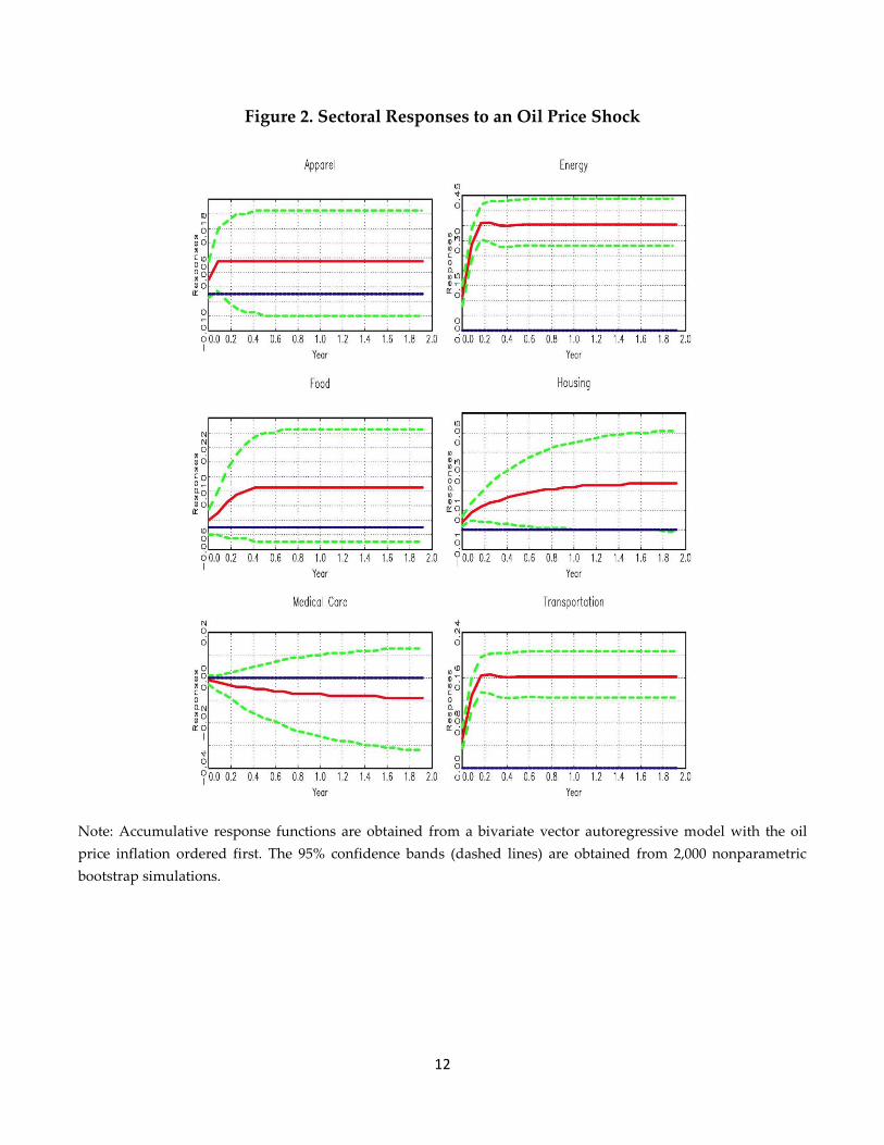
As seen in Figure 2, we obtain mixed responses to the positive oil price shock. We

observed insignificant responses for the apparel, food, and medical care indices, while strong

and significantly positive responses are estimated for the energy and transportation indices.

The significantly positive pass-through effect to the housing price, however, was short term

and lasts only for about one year. In a nutshell, we found that the pass-through effect of the oil

price shock to overall CPI might have been driven by substantial responses of prices in energy-

intensive sectors. In what follows, we investigate the role of economic factors, focusing on the

role of adjustments of consumption due to income changes, which may explain such

heterogeneous responses of CPI sub-indices to the oil price shock.

Figures 1 and 2 around here

3 Responses of the Relative Price

In this section, we study the response of a CPI sub-index relative to the total CPI to the oil

price shock, which is also deflated by the total CPI. Note that a decrease (increase) in the

relative CPI sub-index to a positive real oil price shock implies a relatively weaker (stronger)

response of the CPI sub-index to the response of the total CPI, which might occur when the

composition of consumption goods changes when the oil price increases unexpectedly.

Let and be the real spot oil price and a relative CPI sub-index, respectively. All

variables are expressed in natural logarithms and deflated by the aggregate US CPI. That is,

4

we construct the following bivariate VAR( ) model for relative prices with deterministic

trends.5

( ) (2)

where [ ] [ ], is a diagonal coefficient matrix for the deterministic terms in , ( ) denotes the lag

polynomial matrix, is a vector of normalized underlying structural shocks ( ),

and is a lower triangular matrix that describes the contemporaneous relationships

among and . Again, we obtain the conventional orthogonalized impulse-response

function (OIRF) by Sims (1980) and the variance decomposition analysis is implemented from

this framework. 95% confidence bands are constructed by taking 2.5% and 97.5% percentiles

from 2,000 nonparametric bootstrap simulations.

Responses to the oil price shock are reported in Figure 3. Note that the relative price

(price share) exhibits significantly negative movements at least in the short-run for the apparel,

food, housing, and medical care sub-indices. We observed very persistent upward movements

of relative prices in energy-intensive sectors, that is, the energy and transportation sub-indices.

Our findings are consistent with that of Edelstein and Kilian (2009) in the sense that the

spending adjustment effect plays an important role in determining the price dynamics.

Unexpected changes in the oil price shift not only the supply but also the demand curve of

goods and services to the left due to a decrease in purchasing power of discretionary income.

When the demand for energy is inelastic, unexpected increases in the oil price result in

disposable income for other goods and services. If the oil price shock results in a persistent

negative effect on income growth, consumer spending will be further depressed over time.

5 All eigenvalues are within the unit circle, implying the system is jointly trend stationary.

5

When the demand responds substantially, relative price in that sector is likely to fall, which is

consistent with a limited or weak pass-through effect on prices in less energy-intensive sectors.

Insert Figure 3 around here

We also implement the variance decomposition analysis to see how much variations of

each sub-index are explained by the oil price shock (see Table 1). We observe a dominant role

of the oil shock only for the energy and transportation sub-indices, while limited roles of the

shock were observed for the apparel, food, housing, and medical care sub-indices especially in

the short-run. For example, the oil price perturbation explains only 1.2% of variations in the

one-period ahead forecast of the apparel sub-index, whereas it explains 17.8% for the energy

sub-index. Furthermore, the former is insignificant at the 5% level, while the latter is

significant at any conventional levels. In the longer-run, the oil price shock explains 13.7% of 5-

year ahead forecast of the food sub-index, while 72.3% for the transportation sub-index.

Insert Table 1 around here

Next, we augment the current system to a trivariate VAR model by adding the personal

consumption expenditures (PCE) deflated by the CPI ( ), replacing in equation (2) by , to see if the oil price shock results in a non-negligible adjustment effect

in consumer spending.

We note that all response function estimates of relative prices in Figure 4 are

qualitatively similar to those from the bivariate model. More importantly, we observe

significantly negative responses of the real consumption expenditures in response to the oil

price shock for all cases.6 These findings provide further evidence of substantial role of the

6 We further experimented with an augmented VAR with the industrial production. Results confirm prolonged

recessionary effects over time. All results are available upon request from authors.

6

negative income effect. The variance decomposition analysis from this trivariate VAR models

is reported in Table 2, which is also consistent with that of the bivariate model.

Insert Figure 4 and Table 2 around here

4 Regime-Specific Responses of the Relative Price

We further investigate possibilities of regime-specific responses of CPI sub-indices to the oil

price shock. For this purpose, we employ the following simple threshold trivariate VAR model.

( ) ( ) ( ) ( ) (3)

where , ( ) is an indicator function, is a -period lagged threshold

variable, is the chosen threshold value, and ( ) and ( ) denote lag polynomials in the

upper and the lower regime, respectively.

We use the growth rate of the real industrial production (IP) for the threshold variable

and set which is a conventional value. We employed a grid search method by choosing that minimizes the determinant of the variance-covariance matrix. We trimmed off the

upper and lower 10% of the distribution of IP prior to estimation. Coefficient estimates in the

lower and upper regimes are reported in Table 3, and we also demonstrate regime-specific

response function estimates in Figure 5.7

Note two things about the estimated threshold values. First, estimates are roughly

similar to each other with an exception of the system with the energy sub-index. Second, the

majority of observations belong to the upper regime for most cases except the VAR with the

energy sub-index.

7 We report these regime-specific responses instead of the generalized impulse-response function analysis

proposed by Koop et al. (1996) for more intuitive explanations. These regime-specific responses are conditional

response function estimates from each regime based on an assumption that perturbations are small enough not to

result in changes in regimes during transition period.

7

The one-period lagged oil price affects 4 and 3 sub-indices significantly at the 5% level

in the upper and lower regime, respectively. The effect of the lagged oil price is quantitatively

larger in the lower regime for the energy and the transportation sub-indexes, which seems

reasonable because the income effect may play a more important role when the economy is

relatively worse. Likewise, the lagged oil price has a bigger coefficient in absolute value for the

medical sub-index, which implies that the medical sub-index rises more slowly than the total

CPI when the economy enters a period of downturns. For other sub-indices, we obtained

insignificant contemporaneous effects. We investigate dynamic effects over time via the

impulse-response function estimates in Figure 5.

Regime-specific conditional impulse-response functions during upper regimes (solid

lines) are overall consistent with those from the linear bivariate and trivariate models. This

result is not surprising since about 80% of observations belong to the upper regime.

Several interesting results from response function estimates are as follows. There are

greater responses during the lower growth regime (dashed) compared with those during the

upper growth regime for the energy sub-index. Since observations are split about 42% and 57%

in the lower and higher regime for this index, one cannot ignore the different response

estimates. These greater responses during the low growth regime seem consistent with

Edelstein and Kilian (2009), because the negative income effect would become greater when

the economy is bad, resulting in weaker responses of less energy-intensive product prices

compared with those of more energy-intensive goods prices. The transportation sub-index also

exhibit similar estimates.

The medical care and the food sub-indices overall show greater decreases relative to the

total CPI during the lower regime than the upper regime, which is again consistent with the

income adjustment hypothesis. The response estimates for the apparel and the housing sub-

indices during the low growth regime seem somewhat inconsistent with previous estimates

from linear models. However, since observations during the lower regime for these indices are

only around 20%, we do not attempt to understand these results.

8

Insert Table 3 and Figure 5 around here

5 Concluding Remarks

This paper empirically evaluates the role of spending adjustments when there is an oil price

shock using six CPI sub-indices in the US. We find limited pass-through effects of the oil price

shock on the apparel, food, housing, and medical care CPI sub-indices compared with those on

more energy-intensive industry indices such as the energy and transportation prices.

We propose an explanation for such heterogeneous responses from spending

adjustment effects based on the work of Edelstein and Kilian (2009), who point out a negative

income effect caused by unexpected changes in the oil price. That is, unexpected increases in

the oil price may result in a decrease in the demand for non-energy goods and services when

the demand for energy is inelastic. Decreases in the demand for those goods then would

suppress the degree of the pass-through effect of the oil price shock for those less energy

intensive sector prices but not in more energy intensive sub-indices.

9

References

Barsky, R., & Kilian, L. (2002), “Do we really know that oil caused the great stagflation? A monetary alternative,” in NBER Macroeconomics Annual 2001, Benjamin Bernanke and Kenneth Rogoff (Eds.), 137-183.

Barsky, R., & Kilian, L. 2004. Oil and the macroeconomy since the 1970s. Journal of Economic

Perspectives, American Economic Association, 18(4), 115-134.

Bernanke, B.S., Gertler, M., & Watson, M. 1997. Systematic monetary policy and the effects of

oil price shocks. Brookings Papers on Economic Activity, 91–157.

Colognia, A., & Manera, M. 2008. Oil prices, inflation and interest rates in a structural

cointegrated VAR model for the G-7 countries. Energy Economics, 30(3), 856–888.

Darby, M.R. 1982. The price of oil and world inflation and recession. The American Economic

Review, 72(4), 738-751.

Edelstein, P., & Lutz, K. (2009), “How sensitive are consumer expenditures to retail energy prices?” Journal of Monetary Economics 56, 766-779.

Ferderer, J.P. 1996. Oil price volatility and the macroeconomy. Journal of Macroeconomics,

18(1), 1–26.

Gisser, M., & Goodwin, T.H. 1986. Crude oil and the macroeconomy: Tests of Some Popular

Notions. Journal of Money, Credit and Banking, 18(1), 95-103.

Hamilton, J.D. 1996. This is what happened to the oil price-macroeconomy relationship.

Journal of Monetary Economics, 38, 215 –220.

Kilian, L. 2009. Exogenous oil supply shocks: how big are they and how much do they matter

for the U.S. economy? The Review of Economics and Statistics, 90(2), 216 – 240.

Kilian, L. & Lewis, L.T. 2011. Does the fed respond to oil price shocks? The Economic Journal,

121, 1047–1072.

Kim, H.(2012), “Generalized impulse response analysis: General or extreme?” Auburn Economics Working Paper No. 2012-04.

10

Koop, Gary & Pesaran, M. Hashem & Potter, Simon M., 1996. Impulse response analysis in

nonlinear multivariate models. Journal of Econometrics, 74(1), 119-147.

Korhonen, I. & Ledyaeva, S. 2010. Trade linkages and macroeconomic effects of the price of oil.

Energy Economics, 32, 848–856.

Pesaran, M. H., & Shin Y. (1998), “Generalized impulse response analysis in linear multivariate models,” Economics Letters 58, 17-29.

Sims, C. A. (1980), “Macroeconomics and reality,” Econometrica 48, 1-48.

Zhang, D.Y. 2012. Oil shock and economic growth in Japan: A nonlinear approach. Energy

Economics, 30(5), 2374–2390.

11

Figure 1. Consumer Price Index Response to an Oil Price Shock

Note: Accumulative response functions are obtained from a bivariate vector autoregressive model with the oil

price inflation ordered first. The 95% confidence bands (dashed lines) are obtained from 2,000 nonparametric

bootstrap simulations.

12

Figure 2. Sectoral Responses to an Oil Price Shock

Note: Accumulative response functions are obtained from a bivariate vector autoregressive model with the oil

price inflation ordered first. The 95% confidence bands (dashed lines) are obtained from 2,000 nonparametric

bootstrap simulations.

13

Figure 3. Price Share Responses to an Oil Price Shock

Note: Response functions are obtained from a bivariate vector autoregressive model with the real oil price

ordered first. The 95% confidence bands (dashed lines) are obtained from 2,000 nonparametric bootstrap

simulations.

14

Figure 4. Price Share Responses to an Oil Price Shock: Trivariate Models

Note: Response functions are obtained from a trivariate vector autoregressive model with the real oil price is

ordered first, while the real consumption expenditure is ordered last. The 95% confidence bands (dashed lines)

are obtained from 2,000 nonparametric bootstrap simulations.

15

Figure 5. Regime Specific Impulse-Response Function Estimations

Note: Impulse-response functions are obtained from threshold trivariate vector autoregressive (VAR) models

with the one-period lagged real industrial production growth rate as the threshold variable. We calculated

conditional impulse-response functions from each regime, the low growth regime (dashed) and the high growth

regime (solid), assuming that shocks are small enough not to result in any regime change. We used the Choleski

factor from the whole threshold VAR model.

16

Table 1. Variance Decomposition Analysis for

k Oil Apparel se

k Oil Energy se

1 0.012 0.988 0.011

1 0.178 0.822 0.037

3 0.076 0.924 0.030

3 0.563 0.437 0.047

6 0.140 0.860 0.046

6 0.729 0.271 0.050

12 0.237 0.763 0.072

12 0.833 0.167 0.056

24 0.383 0.617 0.115

24 0.896 0.104 0.060

36 0.479 0.521 0.141

36 0.916 0.084 0.060

48 0.542 0.458 0.155

48 0.925 0.075 0.061

60 0.584 0.416 0.163

60 0.930 0.070 0.061

k Oil Food se

k Oil Housing se

1 0.039 0.961 0.019

1 0.026 0.974 0.017

3 0.129 0.871 0.039

3 0.146 0.854 0.042

6 0.168 0.832 0.051

6 0.179 0.821 0.052

12 0.177 0.823 0.064

12 0.153 0.847 0.055

24 0.165 0.835 0.084

24 0.106 0.894 0.046

36 0.153 0.847 0.098

36 0.108 0.892 0.055

48 0.144 0.856 0.106

48 0.141 0.859 0.078

60 0.137 0.863 0.111

60 0.182 0.818 0.098

k Oil Medical Care se

k Oil Transportation se

1 0.087 0.913 0.025

1 0.119 0.881 0.034

3 0.279 0.721 0.047

3 0.394 0.606 0.050

6 0.356 0.644 0.061

6 0.530 0.470 0.058

12 0.375 0.625 0.086

12 0.630 0.370 0.066

24 0.365 0.635 0.123

24 0.701 0.299 0.071

36 0.354 0.646 0.145

36 0.718 0.282 0.073

48 0.346 0.654 0.157

48 0.722 0.278 0.074

60 0.341 0.659 0.165

60 0.723 0.277 0.076

Note: Variance decomposition analysis is implemented from a bivariate vector autoregressive model with the real

oil price ordered first. is the k-period (month) ahead forecast of the variable x (each sub-index) at time t and

k denotes the forecast horizon in months. Standard errors (se) are obtained from 2,000 nonparametric bootstrap

simulations.

17

Table 2. Variance Decomposition Analysis: Tri-Variate Models

Apparel Energy

k Oil Consum

k Oil Consum

1 0.011 0.989 0.000

1 0.210 0.790 0.000

3 0.073 0.917 0.010

3 0.584 0.415 0.002

6 0.134 0.850 0.016

6 0.735 0.264 0.001

12 0.188 0.799 0.014

12 0.822 0.177 0.001

24 0.225 0.767 0.008

24 0.858 0.137 0.006

36 0.227 0.764 0.009

36 0.859 0.127 0.014

48 0.213 0.769 0.018

48 0.851 0.123 0.026

60 0.193 0.774 0.033

60 0.839 0.121 0.040

Food Housing

k Oil Consum

k Oil Consum

1 0.037 0.963 0.000

1 0.028 0.972 0.000

3 0.125 0.875 0.000

3 0.157 0.812 0.031

6 0.146 0.852 0.002

6 0.180 0.763 0.057

12 0.143 0.841 0.016

12 0.146 0.777 0.077

24 0.130 0.789 0.081

24 0.098 0.811 0.092

36 0.122 0.708 0.171

36 0.089 0.820 0.091

48 0.117 0.630 0.252

48 0.095 0.821 0.084

60 0.117 0.574 0.309

60 0.100 0.823 0.077

Medical Care

Transportation

k Oil Consum

k Oil Consum

1 0.087 0.913 0.000

1 0.138 0.862 0.000

3 0.275 0.723 0.002

3 0.424 0.572 0.005

6 0.351 0.646 0.004

6 0.558 0.435 0.007

12 0.408 0.584 0.008

12 0.670 0.324 0.005

24 0.453 0.527 0.020

24 0.753 0.242 0.005

36 0.465 0.498 0.037

36 0.774 0.220 0.006

48 0.461 0.480 0.059

48 0.781 0.213 0.006

60 0.450 0.467 0.083

60 0.784 0.211 0.006

Note: Variance decomposition analysis is implemented from a trivariate vector autoregressive model with the

real oil price ordered first, while the real consumption expenditure, denoted Consum, is ordered last. is the

k-period ahead forecast of the variable x at time t and k denotes the forecast horizon in months.

18

Table 3. Threshhold Vector Autoregressive Model Estimations

0.953 (0.033) -0.458 (0.411) 0.178 (0.170)

(19.1%) -0.000 (0.002) 1.007 (0.027) -0.011 (0.011)

-0.010 (0.003) -0.023 (0.038) 0.986 (0.016) 0.967 (0.015) -0.169 (0.118) 0.172 (0.056)

(80.9%) -0.003 (0.001) 0.979 (0.008) -0.003 (0.004)

-0.004 (0.001) -0.015 (0.011) 0.996 (0.005)

1.141 (0.042) -0.431 (0.121) 0.004 (0.064)

(42.2%) 0.103 (0.011) 0.714 (0.030) -0.025 (0.016)

-0.023 (0.004) 0.052 (0.011) 0.998 (0.006) 0.884 (0.044) 0.288 (0.118) 0.209 (0.072)

(57.8%) 0.045 (0.011) 0.889 (0.030) -0.009 (0.019)

-0.002 (0.004) 0.002 (0.011) 0.993 (0.007)

0.937 (0.026) 2.550 (0.596) -0.853 (0.219)

(17.7%) 0.001 (0.001) 0.845 (0.034) 0.047 (0.012)

-0.008 (0.002) -0.124 (0.055) 1.016 (0.020) 0.977 (0.010) 0.469 (0.245) 0.001 (0.083)

(82.3%) -0.000 (0.001) 0.968 (0.014) 0.012 (0.005)

-0.002 (0.001) -0.055 (0.023) 1.008 (0.008)

0.968 (0.023) 2.633 (0.960) 0.465 (0.186)

(19.1%) 0.002 (0.001) 0.869 (0.039) -0.018 (0.008)

-0.008 (0.002) -0.150 (0.089) 0.952 (0.017) 0.978 (0.011) 0.372 (0.283) 0.174 (0.058)

(80.9%) -0.000 (0.000) 0.986 (0.011) -0.000 (0.002)

-0.003 (0.001) 0.017 (0.026) 0.994 (0.005)

0.964 (0.043) -0.176 (0.410) 0.000 (0.097)

(19.1%) -0.007 (0.002) 0.949 (0.021) -0.019 (0.005)

-0.016 (0.004) -0.087 (0.038) 0.970 (0.009) 0.964 (0.018) -0.204 (0.176) 0.111 (0.051)

(80.9%) -0.003 (0.001) 0.974 (0.009) -0.007 (0.003)

-0.004 (0.002) -0.021 (0.016) 0.991 (0.005)

1.052 (0.036) -0.988 (0.385) -0.171 (0.115)

(18.7%) 0.019 (0.004) 0.727 (0.043) -0.039 (0.013)

-0.010 (0.003) 0.020 (0.036) 0.982 (0.011) 1.017 (0.020) -0.548 (0.268) 0.054 (0.060)

(81.3%) 0.012 (0.002) 0.856 (0.030) -0.014 (0.007)

-0.006 (0.002) 0.052 (0.025) 1.000 (0.006)

19

Note: Estimates that are significant at the 5% are in bold. One period lagged real consumption growth rate is used

as the threshold variable. Numbers in brackets in the first column are the frequency of observations in each

regime.