How Long Will It Last?Cabinet Termination in Presidential Systems∗

Thiago Silva†

August 29, 2016

Abstract

Studies on presidential democracies show that coalition governments are not a rarephenomenon in presidential systems. But how long do they last? Whether and underwhat conditions are coalition terminations more likely to happen in presidential systems?These are the main questions that I aim to answer in this study. I suggest a theoryframework in which I adapt elements from the literature on parliamentary systems tothe context and specificities of presidential systems. Based on the exclusive powers of thepresident to form and reshuffle cabinets, I expect economic indicators and the evaluationof the president’s job to be crucial factors to predict cabinet termination. By examining82 cabinets from 1978 to 2007 in 10 Latin American democracies, I found that inflation,unemployment, and the fragmentation within the coalition and the party system are themain predictors of cabinet breakdown.

Keywords: Coalition Governments; Cabinet Survival; Cabinet Termination Presidential Systems; LatinAmerica.

∗Paper to be presented at the 112th American Political Science Association Annual Meeting, Philadelphia,PA, USA.†PhD Candidate, Department of Political Science, Texas A&M University, College Station, TX, USA,

77843-4348. Email: nsthiago@tamu.edu

1 Introduction

Contrary to the assumption that the formation of coalition governments would be rare in

presidential systems (Linz, 1990; Mainwaring, 1993), studies on Latin American democracies

(Deheza, 1998; Figueiredo and Limongi, 1999; Lanzaro, 2001; Amorim Neto, 2006a) demon-

strate that this type of government is the standard (Cheibub, 2007; Figueiredo, Salles and

Vieira 2009). Nevertheless, despite the large body of research on the legislative performance

of coalition governments in Latin America, empirical and comparative analyses on coalition

survival in presidential systems remain scant, and important questions remain unanswered:

Why don’t coalitions last the entire presidential term? How long will coalition cabinets last

in presidential systems? Whether and under what conditions are cabinet terminations more

likely to happen in presidential systems?

To answer these questions, in this paper I propose a theoretical framework in which I

adapt elements from the extensive literature on cabinet survival in parliamentary systems

to the context and specificities of presidential systems. I argue that the problem with the

studies on coalition termination1 in presidential democracies is that they do not consider the

possibility that in some contexts it may be more rational for the coalition parties to commit

themselves to the president. If the incumbent is popular and the economy is strong, for

example, members of the coalition may benefit from the president’s popularity, and it would

not be rational for the coalition’s members to leave the government simply because elections

are approaching. Moreover, parties cannot evaluate alternative offers in the formation of the

government’s cabinet, but only the one offered by the president.

Presidents can alter the government coalition over the course of their terms by building a

support base in the legislature, but members of the coalition can also decide to abandon or re-

main in the government based on contextual factors such as the national economic condition,

and the approval ratings of the president. The changes in cabinet due to these factors are

not necessarily influenced by institutional mechanisms, but are due to political and electoral1In this study, by using coalition as cabinet coalition, I use cabinet termination and coalition termination

interchangeably.

1

reasons. Accordingly, in this study I suggest a theory in which the likelihood of cabinet ter-

mination is affected by contextual factors such as inflation, unemployment, economic growth,

and the approval ratings of the president. I also take into consideration important structural

factors, such as the fixed-term of the presidency and how fragmented and polarized is the

political system. These institutional factors are tested in order to examine whether and under

what conditions cabinet terminations are more likely in presidential systems.

By conducting an event history analysis in a longitudinal dataset from 1978 to 2007 that

includes 10 democracies in Latin America, the results in this study show that inflation, un-

employment, and the fragmentation within the coalition and the party system are the main

predictors of cabinet termination.

This paper is structured as follows: In the next section, I present a review of the literature

on coalition termination. This review is strongly influenced by the large literature on parlia-

mentary systems, but an automatic application of parliamentary models to the presidential

context would result in major misconceptions. Thus, I also aim to provide information on

the specificities of presidential systems. In section 3, I present my theory, and, based on the

theoretical model proposed, I suggest four hypotheses to be tested. In section 4, I present

the data and the variables used in this study, and discuss the conducted method to test the

hypotheses. In section 5, I discuss the results of this study, and in section 6, I present my

final comments.

2 Literature Review

According to previous studies on presidential systems, Latin American coalition governments

should either be rare, due to “the perils of presidentialism” (Linz, 1990), or unstable, due to

difficult institutional combinations (Mainwaring, 1993; Stepan and Skach, 1993; Jones, 1995)

and the “tyranny of the electoral calendar” (Altman, 2000a,b).

Linz (1990; 1994) suggests that presidential systems have structural problems such as the

dual legitimacy of the executive and legislative branches, the increased likelihood of inter-

branch conflict, and the lack of an institutional mechanism to resolve these conflicts. The

2

“difficult combination” hypothesis (Mainwaring, 1993) implies that the inter-branch conflict

and the legislature’s non-cooperative behavior would be aggravated by the combination of a

strong president with a multiparty system. The “tyranny of the electoral calendar” hypothesis

(Altman, 2000b), in turn, suggests that as new elections approach, members of the coalition

will try to distance themselves from the president in order to avoid paying the costs associated

with the government’s policies. Therefore, because the coalition’s parties would be better off

competing in elections alone, they would abandon the government before the end of the

presidential term (Chasquetti, 1999; Altman, 2000a,b).

However, studies comparing parliamentary and presidential systems (Cheibub and Limongi,

2002; Cheibub, Przeworski and Saiegh 2004) suggest that the incentives for coalition formation—

such as increasing legislative strength and policy influence—are present in both government

systems. Therefore, there is no reason to believe in an inherent structural problem within

presidential systems when the same behavioral premises and similar decision-making rules

are observed in both systems (Cheibub and Limongi, 2002, 2011; Cheibub, Elkins and Gins-

burg 2014). Empirical studies on Latin American democracies (Deheza, 1998; Figueiredo and

Limongi, 1999; Amorim Neto, 2000a, 2006a; Chasquetti, 1999; Lanzaro, 2001; Alemán and

Tsebelis, 2011) support this argument, and have revealed that coalition governments have

been the most frequent and effective way to address and resolve the president’s problem of

legislative minority support. Therefore, coalition government should not be considered a rare

phenomenon in presidential systems (Cheibub and Limongi, 2002; Cheibub, Przeworski and

Saiegh 2004; Cheibub, 2007; Figueiredo, Salles, and Vieira 2009).

Also, some scholars (Shugart and Carey, 1992; Mainwaring and Shugart, 1997) called

attention to the diversity of presidential systems and suggested some virtues of these sys-

tems that are usually overlooked by the literature. According to Shugart and Carey (1992),

the fixed-term nature of the presidency can be seen as an attribute of predictability within

presidential systems, and not as something inherently problematic. Mainwaring and Shugart

(1997) reveal that Linz (1990; 1994) overlooked the possibility of conflict in parliamentary

systems, as well as underrated the positive features of presidential systems. Also, the mutual

3

independence of the executive and legislative branches can favor the system of checks and

balances between these powers (Melo and Pereira, 2013).

Nevertheless, the analysis on Latin American presidential democracies are mostly descrip-

tive case studies concerned with either demonstrating that coalition governments are not rare

in the region, or to evaluate the legislative success of coalition governments under presidential

systems. Such examples can be seen in studies on Brazil (Figueiredo and Limongi, 1999),

Uruguay (Chasquetti, 1999), Chile (Siavelis, 2000), Argentina (Novaro, 2001), and Bolivia

(Mayorga, 2001). In contrast to the extensive literature on parliamentary systems (Strøm,

1984, 1988; Schofield and Laver, 1985; Laver and Schofield, 1990; Laver and Shepsle, 1994;

Lupia and Strøm, 1995; Grofman and van Roozendaal, 1997; Strøm, Kaare, Wolfgang Müller,

and Torbjörn Bergman, 2008), theoretical models and empirical comparative analysis on cab-

inet survival in presidential systems remain underdeveloped.

The theories developed regarding cabinet survival and termination under parliamentary

systems consider the bargaining environment complexity (Laver and Schofield, 1990; Alt and

King, 1994), ideological diversity and polarization (Warwick, 1992, 1994), institutional mech-

anisms such as investiture and no-confidence vote (Strøm, 1988), external environments such

as economic conditions (Robertson, 1983a,b, 1984; Warwick, 1992; Narud, 1995), strategic

timing of elections and calculus of alternative coalitions (Grofman and van Roozendaal, 1994;

Lupia and Strøm, 1995), strategies to reduce the prime minister’s agency loss (Indridason and

Kam, 2008), and structural attributes such as the size and number of political parties (Strøm,

Müller and Bergman 2008; Bergman and Hellström, 2015).

Some of the theories developed for parliamentary systems are clearly not applicable to

presidential contexts. Presidential systems have some specific rules on coalition formation

and ministerial reshuffle that should not be overlooked: 1. Presidents have constitutional

powers to form and reshuffle the government’s cabinet (Amorim Neto, 2000a; Figueiredo,

2007); 2. Presidents are always the formateur in the government formation game (Cheibub,

Przeworski, and Saiegh, 2004; Alemán and Tsebelis, 2011; Silva, 2016) and; 3. Due to their

independency from the legislature and the absence of the vote of no confidence, presidents

4

have constitutionally fixed terms, and, other than in exceptional cases, presidents remain in

power even under adverse legislative conditions (Shugart and Carey, 1992; Mainwaring, 1993;

Altman, 2000b; Cheibub, Przeworski and Saiegh 2004; Cheibub, 2007).

The hypothesis of “the tyranny of the electoral calendar” is directly related to the specifici-

ties of the presidential systems, particularly regarding presidential and legislature fixed-terms.

The term “tyranny of the electoral calendar” was coined by Altman (2000a), but the expecta-

tion is similar in all cited studies: as the next election approaches, parties have fewer incentives

to join or remain in the government, and therefore cabinet termination should be more likely,

given the impending elections (Chasquetti, 1999; Altman, 2000a; Alemán and Tsebelis, 2011).

Although Altman considers that other covariates—such as economic and ideological factors—

can affect cabinet duration, the author sustains that “nonetheless, whether a party remains

in the executive coalition is subject to the tyranny of the electoral calendar” (Altman, 2000a,

p. 19). Thus, at the end of the president’s term, members of the coalition would mainly be

concerned with electoral gains, and behave as office- and vote-seeking actors (Altman, 2000b,

p. 268).

The rationale behind “the tyranny of the electoral calendar” is that members of the coali-

tion should try to distance themselves from the president in order to avoid paying the costs of

being associated with the incumbent government. Moreover, in presidential systems there is

no mechanism to force coalition members to support the president in the legislative branch.

Thus, the president should have, at most, only control over members of her own party and not

on the other members of the coalition (Chasquetti, 1999). Also, as already mentioned, pres-

idents remain in power even under adverse legislative conditions (Shugart and Carey, 1992;

Mainwaring, 1993; Altman, 2000b). Therefore, the proximity of the elections should create

strong incentives for members of the coalition to leave the cabinet.

However, the “tyranny of the electoral calendar” hypothesis neglects the possibility that

parties’ identification with the president can bring electoral benefit for the members of the

coalition. As stated by Cheibub and Limongi (2002, p. 158), there is no reason to assume

that, under presidential systems, being part of the government “brings no electoral benefit

5

and that presidents are not able to transfer votes for the politicians who support them.”

Heading a portfolio allows governing parties to have discretion within specific policy domains

(Druckman and Thies, 2002; Falcó-Gimeno and Indridason, 2013). Moreover, being part

of a government cabinet can give parties visibility and influence regarding important policy

consequences (Freitas, 2013; Araújo, 2016).

Therefore, the decision to join the government involves not only electoral losses, but also

potential gains for the members of the coalition (Cheibub and Limongi, 2002; Freitas, 2013;

Araújo, Freitas and Vieira 2015). There is no reason to suppose that only under presidential

systems do the losses exceed the gains for coalition’s members (Limongi, 2003). In addition,

even if we supposed that legislators always want to oppose the president, in presidential

systems the chief of the executive branch usually controls important resources for legislators,

such as patronage, budget or the policy agenda (Shugart and Carey, 1992; Mainwaring and

Shugart, 1997; Figueiredo and Limongi, 1999). The control over these resources thus puts the

president in a favorable position to bargain cooperation with legislators.

In this paper, I challenge the studies so far conducted on coalition termination in presi-

dential multiparty systems. I propose a theoretical framework in which I adapt elements from

the extensive literature on cabinet survival in parliamentary systems to the context of pres-

idential systems. I agree that specificities within presidential system changes the incentives

to form and sustain the government’s coalition (Chasquetti, 1999; Altman, 2000a; Alemán

and Tsebelis, 2011). However, I argue that factors that make the termination of a coalition

government more likely in presidential systems are neither due to structural problems of this

system of government nor due the “tyranny of the electoral calendar.” The reason, theoreti-

cally suggested and empirically tested in this study, is that parties cannot evaluate alternative

offers in the formation of the government’s cabinet, but only the one offered by the president.

This puts the president in a privileged position, and consequently makes the evaluation of the

president’s performance and other contextual factors crucial elements in the parties’ calculus

whether or not to stay in the government.

6

3 Theory and Hypotheses

Although this research takes cues from the literature on parliamentary systems, an automatic

application of theoretical models from the parliamentary literature to the presidential context

would result in major misconceptions. Presidents have some exclusive powers on coalition

formation and the dynamics of ministerial reshuffling in presidential systems, which are: 1.

Constitutional prerogative powers to form and reshuffle the government’s cabinet; 2. Ex-

clusivity as the formateur in the coalition’s formation, and; 3. Constitutionally-fixed terms,

remaining in power even under adverse legislative conditions. In this sense, parties cannot

evaluate alternative coalition offers in presidential systems, but only the one offered by the

president. Moreover, if the parties decide to not participate in the government by rejecting

the president’s offer, they have to wait until the next election in order to receive benefits from

being part of the government (Alemán and Tsebelis, 2011).

Therefore, in this paper I suggest a theory in which the end of coalition governments

depends on contextual factors directly related to government’s performance such as economic

conditions—inflation, unemployment, and economic growth—and the approval rating of the

president. This theory is based on the argument that the exclusive powers of the president to

form and reshuffle cabinets restricts the options for potential parties that will comprise the

government, and makes the evaluation of the president’s approval rating and other contextual

factors crucial elements in the parties’ decision to participate or not in the coalition. Presidents

can alter the government coalition over the course of their terms by building a support base

in the legislature, but members of the coalition might decide to abandon or remain in the

government based on contextual factors, such as the national economic condition and the

public’s approval rating of the president. The changes in government due to these factors

are not necessarily influenced by institutional mechanisms but due to political and electoral

reasons.

Important structural factors—such as the fixed term of presidents, and how fragmented

and polarized is the political system—which are commonly presented by the literature as

7

important factors on cabinet formation and termination (Altman, 2000a,b; Amorim Neto,

2006a; Alemán and Tsebelis, 2011) are also considered here.

According to the theory here suggested, I assume that politicians behave both as office-

seeking and policy-seeking actors. Although it is difficult to distinguish these behaviors empir-

ically, as noted by Druckman (2002, p. 761), “the assumption that politicians care only about

office seemed unjustifiably restrictive.” Maybe policy matters only because it leads to votes

and, consequently, to offices, but here it is assumed that policy consideration still influences

coalition formation and survival.

Following the theory stated above, four hypotheses will be tested in this study:

Hypothesis 1. As the country’s inflation rate increases, a higher likelihood of cabinet

termination and, consequently, a shorter duration of the cabinet is expected.

Hypothesis 2. As the country’s unemployment rate increases, a higher likelihood of cabinet

termination and, consequently, a shorter duration of the cabinet is expected.

Hypothesis 3. As the presidential approval rate increases, a reduction in the likelihood of

cabinet termination and, consequently, a longer duration of the cabinet is expected.

Hypothesis 4. As the country’s GDP growth increases, a reduction in the likelihood of

cabinet termination and, consequently, a longer duration of the cabinet is expected.

4 Concepts, Data, and Methods

With some important exceptions (Amorim Neto, 2000a, 2006a; Altman, 2000b; Alemán and

Tsebelis, 2011; Martínez-Gallardo, 2012, 2014), studies of coalitions under presidentialism

remain largely descriptive (Lanzaro, 2001; Figueiredo and Limongi, 2007; Figueiredo, 2007)

and usually lack a comparative perspective, making generalizations from theoretical models

rather difficult. In order to model the likelihood of coalition termination, in this study I

will conduct an event-history analysis (Cox and Oakes, 1984; Box-Steffensmeier and Jones,

2004) using a dataset that is comprised of data from 10 Latin American democracies, from

8

1978 to 2007.2 The justification for the use of these cases is based on data availability, and

on definitions for three main concepts of the analysis: democracy, presidential systems, and

coalition government.

4.1 Concepts: Democracy, Presidential System, and Coalition Gov-

ernment

For the classification of a democratic regime, I use the definition suggested by Przeworski, Al-

varez, Cheibub and Limongi (2000), and further developed by Cheibub, Gandhi and Vreeland

(2010, p. 69):

1. The chief executive must be chosen by popular election or by a body that was itself

popularly elected;

2. The legislature must be popularly elected;

3. There must be more than one party competing in the elections; and

4. An alternation in power under electoral rules identical to the ones that brought the

incumbent to office must have taken place.

This classification has the advantages of being comprehensive on classifying worldwide

political regimes in a minimalist way, related to the particular research question that is being

addressed in this study (Collier and Adcock, 1999), and, in practice, this classification is

strongly correlated with other common measures of democracy such as those developed by

the Freedom House and the Polity IV Project.

Presidential systems are defined according to the commonly used concept developed by

Shugart and Carey (1992, p. 19-20):

1. The chief executive is elected by popular vote or by a body that was itself popularly

elected;2The presidential systems and the time range included are: Argentina (1989-2001), Bolivia (1982-2001),

Brazil (1985-2007), Chile (1990-2004), Colombia (1978-2000), Ecuador (1979-1999), Panama (1990-2002), Peru(1980-1991), Uruguay (1985-2003), and Venezuela (1992-1999).

9

2. The terms of the chief executive and the assembly are fixed, and are not contingent on

mutual confidence;

3. The chief executive selects and removes the members of the cabinet; and

4. The chief executive has some constitutionally granted lawmaking authority such as veto

power.

Finally, for coalition government I adopt a minimalist definition: a coalition government

is present when at least two parties hold cabinet portfolios. The criterium to define the

demarcation of the end of a cabinet is also very straightforward: Any changes in the set

of parties holding cabinet membership. Following Laver and Schofield (1990, p. 129), it

is important to distinguish two kinds of coalitions: a government (portfolio) coalition, a

set of parties that receive ministerial portfolios and formally support the government, and, a

legislative coalition—that is, a set of parties that ensure votes for the government in congress in

order to approve the president’s agenda. These coalitions can be the same, but not necessarily

so. Parties can support the president in the legislative branch even if they do not hold cabinet

portfolios. Thus, in this study, I am concerned with government coalitions.

One last caveat: The use of the term cabinet termination instead of cabinet duration or

ministerial turnover is justified to emphasize a deliberate decision of specific political actors

(i.e. a coalition’s members). According to Grofman (1997, p. 423-424), cabinet duration

emphasizes that which happens, while cabinet termination emphasizes “those who are making

things happen and invites a concern for why they are choosing to act.” In this sense, a cabinet

turnover or reshuffle can happen even in the absence of cabinet termination, e.g. when the

president changes the ministers, but the set of parties composing the cabinet does not change.

4.2 Data: Duration of Cabinets, Economic Indicators, and Political

Institutions

The dataset used in this study comprises 82 cabinets from 1978 to 2007, and was built from

political data provided by Amorim Neto, updated with data from the Brazilian Center of Anal-

10

ysis and Planning (CEBRAP), and supplemented with economic data from The World Bank

and the Executive Approval Project (EAP).3 The specified model for testing the hypotheses

of this study, explained in detail in next section, is composed of one dependent variable, four

main independent variables, and seven independent variables for control as described below.

Dependent Variable

Cabinet’s durability. The dependent variable is the durability of the cabinets, as measured

by the number of days that the cabinet survived. By having a cabinet for each country as

the unit of analysis, each of the cabinets has a start date and an end date, which allows the

measurement of the durability of each cabinet. As an example, since its recent democratization

in 1990 to the last data available in 2004, Chile has had five different cabinets. The first Chilean

cabinet, during the presidency of Patricio Azócar (1990-1994), lasted 934 days (that is, the

difference between the end date and the start date of the coalition). The same operation was

conducted for each cabinet in every country included in the analysis. The average duration

of the cabinets in the sample is 585.39 days, with a standard deviation of 483.18 days.

The less durable cabinet, with only 30 days, started in June 1986 and was the second

cabinet formed by Ecuadorian President León Febres Cordero. The most enduring cabinets

lasted 1826 days: the first cabinet formed by Uruguayan President Luis Alberto Lacalle, which

started in March 1990, and the first cabinet formed in the second term of Venezuelan President

Rafael Caldera, which started in February 1994.

Independent Variables

By considering the lagged effects of economic indicators and the president’s approval rating

on a cabinet’s durability, all main independent variables were either lagged by one year, or by

one quarter, as described below. It is important to note that the year of reference for lagging

the variable is the year of the dissolution of the cabinet. For example, if a cabinet ends on

year t, the economic information used is the one for t− 1.

Inflation. This variable is a measurement of the consumer price index (CPI), reflecting3The complete data source can be viewed in Appendix A of the Appendix Material. Summary statistics

can be viewed in Appendix B of the same supplementary material.

11

the quarterly percentage change in the cost to the average consumer of acquiring a basket of

goods and services. In the sample, this variable has a mean value of 22.71 percent, with a

standard deviation of 43.45 percent. The minimum value of the sample is -0.58 (Bolivia in

the first quarter of 2001) and the maximum value is 204.54 (Peru in the last quarter of 1988).

The period of hyperinflation in Latin America (from 1985 to 1995) presents disproportionate

values for this variable (with a median = 5.18, seventy-five percent of the values are between

-0.57 and 14 percent, and only 17 observations have a value for inflation greater than 14).

This makes the distribution of the variable extremely skewed, and for this reason the variable

inflation was log transformed.4

Unemployment. This variable refers to the quarterly share (percentage) of the labor force

that is without work but available for and seeking employment. The average unemployment

rate among the countries included in this analysis is 9.29 percent, with a standard deviation of

3.56 percent. The lowest unemployment rate in the sample is 3.40 (Brazil in the last quarter

of 1989), and the highest value is 19.82 (Panama in the first quarter of 1983).

GDP Growth. Annual percentage growth rate of gross domestic product (GDP) at market

prices, based on constant 2005 U.S. dollars. The mean value of this variable in the sample is

2.69 percent, with a standard deviation of 4.31 percent. The variable ranges from a minimum

value of -11.70 (Peru in 1990) and a maximum value of 11.94 (Argentina in 1992).

President’s Approval Rating. This variable measures the presidential job approval based on

country-specific surveys that included the question, “Do you approve or disapprove of the way

that [name of the chief executive] is handling his/her job as [title of executive position]?”5 The

mean value of this variable is 43.30 percent, with a standard deviation of 11.91 percent. The

least-popular president in the sample is the Peruvian President Fernando Belaúnde Terry in

1984 (14.93 percent), and the most-popular president in the sample is the Colombian President

César Gaviria Trujillo in 1992 (69.60 percent).4The distributions of the variables—including the distribution for the log transformed inflation—can be

viewed in Appendix D of the Appendix Material.5In order to deal with the transformation of disparate job approval series into data comparable across

administrations, countries, and time, the original authors of the dataset (Carlin, Martínez-Gallardo, andHartlyn 2012) conducted a methodology based on estimating country-specific measurement models.

12

Control Variables

Cycle. This variable measures the elapsing of the president’s term, expressed as 1− Te−TcaTco

.

Where Te = the year the president’s term ends, Tca = the current year of the president’s term

according to the cabinet i, and Tco is the fixed number of years of the president’s term as

defined by the country’s constitution. As an example of a presidential term of four years, a

value of 0.25 refers to the first year of the president’s term, 0.5 is the second year, 0.75 is the

third year, and 1 refers to the last year of the president’s term.

As mentioned before, an important part of the literature on coalition termination suggests

that as a new election approaches, the likelihood of a cabinet termination will be greater (Alt-

man, 2000a,b). Chasquetti (1999) states that the fixed terms of the president, vice-president

and legislatures seem to be decisive for the duration and stability of cabinets, because parties

that compose the coalition are fully aware of the electoral calendar, and thus maintaining

a coalition should be a function of the temporal distance of the national election (Altman,

2000b, p.278n1). Therefore, according to the “tyranny of the electoral calendar” hypothesis,

it is expected that the more advanced the presidential term (in a temporal sense), the higher

the likelihood of a cabinet termination. Based on the theory proposed in this study, I expect

no relationship between the elapsing of the president’s term and the cabinet termination.

Size of the coalition. This variable refers to the number of parties represented in the

cabinet, i.e. the fragmentation of the coalition. In the sample, this variable has a mean of

3.5 parties composing the coalition, with a standard deviation of 1.62 parties. The smallest

coalitions in the sample are those formed with two parties (26 observations), and the three

biggest coalitions are composed of eight parties—the first (2003) and second (2004) coalitions

formed in the first term of the Brazilian President Lula da Silva, and the first coalition (2007)

formed by Lula da Silva in his second term.

Studies on parliamentary systems found that the number of parties in the cabinet has

a significant and negative impact on cabinet durability (Taylor and Herman, 1971; Sanders

and Herman, 1977). By considering that more parties in the cabinet can lead to more conflict

within the coalition among the governing parties, the same outcome is expected in presidential

13

systems: as the number of parties in the cabinet increases, the likelihood of a cabinet’s

termination will also increase.

President’s Legislative Power (IPIL). Presidential systems vary considerably in the degree

of legislative powers that constitutions grant to the president (Shugart and Carey, 1992). In

order to measure the legislative power of the presidents, I use the legislative institutional power

index (IPIL) developed by Montero (2009). This measurement aggregates five dimensions:

1. The president’s capacity to initiate legislation; 2. The president’s capacity to form and

regulate legislative committees; 3. Symmetry of bicameralism; 4. Presidential veto powers,

and; 5. The president’s decree power and extraordinary prerogatives. The IPIL index ranges

from 0 to 1, where values close to 1 indicate democracies in which presidents have large

institutional prerogatives to influence the legislative activity, i.e. the president’s dominance

over the lawmaking process. The value 0 of the index, in turn, indicates democracies in which

the legislative branch has fewer obstacles to intervene on legislation process, i.e. dominance

of the legislative branch over the lawmaking process.

In the sample, the average for this variable indicates a very balanced lawmaking process

between the president and the legislative branch—a mean of 0.50, with a standard deviation

of 0.08. Nevertheless, a look at specific cases in the dataset show important variance on this

index. In the sample, the president with the least legislative power is the Venezuelan President

Rafael Caldera in his second term in 1994 (IPIL = 0.28), and the president with the highest

legislative power is the Chilean President Ricardo Lagos in 2000 (IPIL = 0.71).

This variable is included in the model based on the aforementioned assumption that politi-

cians behave both as office-seeking and policy-seeking actors. Following Strøm’s argument

(1990), parties can leave the government if being dissociated with the government can increase

a party’s ability to influence policy in the legislature. Therefore, it is expected that the greater

the president’s legislative powers, the smaller the likelihood of a cabinet termination—thus,

the cabinet duration is longer, because the governing parties cannot exert a greater influence

on the policy agenda outside the coalition.

Ideological Dispersion. This variable measures the ideological heterogeneity of the cabinets

14

or polarization, i.e. the ideological distance between the furthest-left party represented in the

cabinet to the furthest-right party represented in the cabinet. Following Coppedge (1997),

Saez and Freidenberg (2001) and Neto (2006a), each governing party was assigned to a numeric

value (from -1 to 1) in a left-right ideological continuum: Left = -1; center-left = -0.5; center

= 0; center-right = 0.5, and; right = 1. Thus, the ideological dispersion of the cabinet can be

expressed as |Pfl − Pfr|, where Pfl = the ideological position on the left-right continuum of

the furthest-left party represented in the cabinet, and Pfr = the ideological position on the

left-right continuum of the furthest-right party represented in the cabinet. The variable thus

ranges from 0—absence of ideological heterogeneity, or a cabinet ideologically homogeneous—

to 2—maximum ideological heterogeneity.

In the sample, there are 16 homogeneous cabinets, and nine observations with the maxi-

mum heterogeneity value. Ideologically homogeneous cabinets are less vulnerable to conflict

and disagreements on policy choices. In other words, the conflict of interest within the coali-

tion intensifies as the ideological dispersion of the cabinet increases, which therefore increases

the polarization of the cabinet. Thus, I expect that the higher the ideological dispersion, the

higher the likelihood of a cabinet termination.

Majority Status. A dichotomous variable indicating that the coalition government has the

majority of seats in the legislative branch. As the opportunity for forming coalition govern-

ments depends on the partisan distribution of seats in the legislature (Cheibub, Przeworski,

and Saiegh, 2004), when the parties holding portfolios have less than 50 percent of the legisla-

tive seats, the coalition is considered a minority coalition (and the variable receives a value

of 0). When the governing parties have more than 50 percent of the legislative seats, the

coalition is considered a majority coalition (and the variable receives a value of 1). Sixty-one

percent of the cabinets included in the sample were cabinets with a majority status.

In order to increase the chance of having her policy agenda approved in the legislature,

the president seeks a higher support of voters among the legislators in the legislative branch.

In other words, when the coalition only forms a minority in congress, the president’s agenda

becomes more unlikely to be approved. Thus, the expected strategy of the president to

15

overcome this problem is to distribute portfolios to more parties, increasing the coalition size

or changing the set of parties that compose it. If the president’s party, combined with the

other governing parties, already have the majority in the legislative branch, the president has

no incentives to change or add more parties to the coalition. In this sense, in the presence of

a coalition with a majority status, I expect that a cabinet termination is less likely.

Cabinet Coalescence Rate. One of the factors suggested by the literature in explaining

the durability of cabinets in presidential systems is the deviation from the proportionality

between the number of ministries held by the governing parties and the number of legislative

seats these parties hold in the legislature (Amorim Neto, 2006a). In this study, I use the

cabinet coalescence rate suggested by Neto (2006a; 2006b) to measure the proportionality of

portfolio distribution, that can be expressed as:

Coalescence = 1−∑ni=1(|si − pi|)

2

Where si= the percentage of legislative seats governing party i holds when the cabinet is

appointed, and; pi = the proportion of portfolios governing party i receives from the total of

available portfolios.

The coalescence rate varies between 0—no correspondence between cabinet shares and leg-

islative seats—and 1—perfect correspondence between cabinet shares and legislative weights.

In Neto’s definition (2000b, p. 4), cabinet coalescence “measures how the distribution of cab-

inet posts is roughly weighed vis-à-vis the dispersion of legislative seats across the legislative

contingent of the parties joining the executive.”

The cabinets included in the sample have a very high coalescence rate, with a mean of

0.94, and a standard deviation of 0.05. The less proportional cabinet was the first cabinet

formed by the Uruguayan President Luis Herrera in 1990 (coalescence = 0.74), and a perfect

proportional cabinet (coalescence = 1) was formed by the Colombian President Cesár Trujillo,

also in 1990.

According to Neto (2000a), the more proportional the distribution of portfolios among the

16

coalition’s members—based on their legislative strength—the higher is the legislative discipline

of these members. Thus, it is expected that the greater the cabinet coalescence, the less likely

is a cabinet termination. This makes sense, because if the government is receiving support

from the parties that comprise the coalition, there is no incentive, ceteris paribus, for the

president to change the cabinet.

Effective Number of Parties (ENP). This variable is the Laakso and Taagepera’s (1979)

measurement of the fragmentation of the party system in the legislative branch. That is,

ENP = 1∑n

i=1 s2i

, where si = percentage of legislative seats the governing party i holds when

the cabinet is appointed. The mean value for this variable in the sample is 5.36 parties, with

a standard deviation of 2.27 parties. The less fragmented party system is Colombia’s in 1986

(ENP = 1.98), and the most fragmented party systems is Brazil’s between 1992 and 1993

(ENP = 9.34).

The higher the legislative fractionalization, the lower the president’s party size (Mainwar-

ing, 1993; Mainwaring and Shugart, 1997; Jones, 1995), and consequently, the greater the

incentive for the president to form coalitions (Chasquetti, 2001; Cheibub, 2007). Also, ac-

cording to Chasquetti (2001), an extremely fragmented system (ENP > 4) should be more

problematic for government stability in presidential systems due to less legislative support for

the president. Thus, I expect that the higher the legislative fractionalization, the higher the

likelihood of a cabinet termination.

4.3 Method: The Cox Proportional Hazards Model

When the duration of the presidential cabinets—measured by the number of days the cabinet

lasts until it terminates—is used as the dependent variable, traditional regression techniques

such as OLS-type should be avoided (Box-Steffensmeier and Jones, 2004). First, because the

dependent variable is the duration, it cannot assume negative values. The time to failure or

the time to the termination of the event is thus always positive. But more importantly, the

problem with using OLS to analyze event history data lies with the assumed distribution of

the residuals. In linear regression, the residuals are assumed to be distributed normally, but

17

the assumption of normality of time to an event may be unreasonable. It is unreasonable, for

instance, if we are thinking about an event that has a likelihood of terminating instantaneously

that is constant over time. In that case, the distribution of time would follow an exponential

distribution.

In this sense, a common approach to estimate duration models is to assume a probability

distribution function for the duration of the event, for example, a Weibull, an exponential,

or a logistic distribution, and estimate the probability for the duration with the method of

maximum likelihood. King, Alt, Burns and Laver (1990) and Warwick (1992), for instance,

used parametric methods to understand coalition durations in parliamentary systems. Both

studies had strong theoretical expectations regarding the distribution of the residuals. The

downside of this approach is that the results are quite sensitive to the chosen distribution

function, and if the distribution of failure times is parameterized incorrectly, then the inter-

pretations afforded by parametric models could be misleading and may not make substantive

sense (Box-Steffensmeier and Jones, 2004).

The theory developed in this study is less focused on the notion of time-dependency, and

more focused on the relationship between the cabinet duration and independent variables of

theoretical interest that vary over time. Thus, in order to estimate the model of cabinet

duration, I use the Cox proportional hazards model with time-varying covariates (Cox, 1972;

Cox and Oakes, 1984; Fisher and Lin, 1999; Box-Steffensmeier and Jones, 2004; Martinussen

and Scheike, 2006; Thomas and Reyes, 2014). The advantage of this approach is that we can

leave the particular distribution form for the duration dependency unspecified,6 and it has

been shown to be preferable on both substantive and statistical grounds to parametric models

(Box-Steffensmeier and Jones, 2004, p. 48).7

6The Cox model is considered a “semi-parametric” model. As described by Box-Steffensmeier and Jones(2004, p. 49), “the (ordered) duration times are parameterized in terms of a set of covariates, but the particulardistributional form of the duration times is not parameterized.”

7The Cox model is also preferred for dealing with right-censoring data—subjects that we do not or cannotobserve long enough for all of them to fail. In the sample data I am using, however, there is no censoring; thefull duration time of cabinets are observed. Nevertheless, left-truncation could be present in the data whenhistory prior to the first observed cabinet in a country is unobserved. The fact that only Latin Americanpresidential systems are included in this study minimizes this problem, because the first observation for eachcountry in the dataset is usually the first cabinet formed in the current democratic era of the country (any

18

The specification of the full model to be estimated is:

hi(t) = h0(t)exp(β1log(inft) + β2unempt + β3presappt + β4GDPt + x′iα) (1)

Where hi(t) is the hazard function for cabinets’ duration—the dependent variable; h0(t) is the

baseline hazard function—a term that depends on time, but where the independent variables

= 0; the main time-varying independent variables (subscripted with t) inflation (log(inf)),

unemployment (unemp), presidential approval rating (presapp), and GDP growth (GDP) enter

in the model linearly with parameter estimates vector β, and; x′i is a vector of observations on

the control variables with parameter estimates vector α. There is no error term in the equation,

because the randomness is implicit to the survival process. Also, because the baseline hazard

rate is left unspecified, the result from the Cox regression model contains no constant term.

This term is “absorbed” into the baseline hazard function h0(t), and for this reason the method

for estimation of the Cox regression model is called maximum “partial” likelihood (Cox, 1975).

5 Results and Discussion

In interpreting the coefficients of a Cox proportional hazards model, the dependent variable

is the hazard rate of the duration of the cabinet. In other words, the hazard rate refers to the

likelihood that a cabinet will terminate at a particular point in time, given that it has not

yet fallen. Therefore, higher hazard rates—positive estimate coefficients—represent a higher

likelihood and, consequently, a shorter duration of the cabinet. Negative estimate coefficients,

in turn, represent a reduction in the likelihood of termination, and consequently, a longer

duration of the cabinet.

Table 1 presents estimate coefficients for four Cox regression models. Due to 10 missing

values in the independent variable “presidential approval rate,” in the first model I decided to

remove this variable in order to keep all observations. The second model is the full model, as

depicted in Equation 1 above. Latin American presidential systems are political and socially

coalition formed in country’s non-democratic period is not included in the analysis).

19

diversified, and thus generalizing the region’s governments can lead to unreliable results. In

order to control for country specificities, I also present the estimates for the first model with

country fixed-effects (Model 3) and for the second model with country fixed-effects (Model

4). To echo Schofield and Laver’s argument (1985, p. 143) for the parliamentary context,

“differences between countries are at least as significant as those between theories.”8

By exponentiating Cox estimates from Table 1, the coefficients turn into the metric of

hazard ratios, and with this we can make better substantial inferences. Table 1 presents the

results in terms of the hazard ratio italics. As such, hazard ratios greater than 1 imply that

the likelihood (or hazard) of cabinet termination increases as the value of the independent

variable increases, thus resulting in a shorter cabinet duration. Hazard ratios smaller than 1,

in turn, imply that the likelihood (or hazard) of cabinet termination decreases as the value of

the independent variable increases, thus resulting in a longer cabinet duration. In contrast,

hazard ratios close to 1—as in the case of the parameters for “GDP growth” and “presidential

approval”—imply that the hazard rate is essentially invariant to changes in the independent

variable, i.e. the coefficient has no effect on increasing (or decreasing) the hazard of cabinet

duration.

8In order to save space, the non-significant results for the fixed-effects terms for countries were omittedfrom Table 1. The results for these terms can be viewed in Appendix F of the Appendix Material.

20

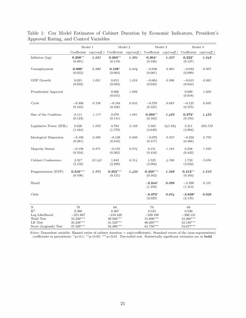
Table 1: Cox Model Estimates of Cabinet Duration by Economic Indicators, President’sApproval Rating, and Control Variables

Model 1 Model 2 Model 3 Model 4Coefficient exp(coeff.) Coefficient exp(coeff.) Coefficient exp(coeff.) Coefficient exp(coeff.)

Inflation (log) 0.208∗∗ 1.231 0.263∗∗ 1.301 0.204∗ 1.227 0.222∗ 1.249(0.091) (0.119) (0.106) (0.127)

Unemployment 0.096∗ 1.101 0.108∗ 1.114 −0.038 0.963 −0.033 0.967(0.052) (0.064) (0.081) (0.099)

GDP Growth 0.021 1.021 0.015 1.016 −0.004 0.996 −0.015 0.985(0.032) (0.033) (0.043) (0.044)

Presidential Approval 0.006 1.006 0.009 1.009(0.015) (0.018)

Cycle −0.306 0.736 −0.184 0.832 −0.379 0.685 −0.125 0.882(0.410) (0.456) (0.425) (0.475)

Size of the Coalition 0.111 1.117 0.078 1.081 0.393∗∗ 1.482 0.373∗ 1.452(0.123) (0.141) (0.162) (0.194)

Legislative Power (IPIL) 0.626 1.870 0.784 2.189 5.505 245.894 5.311 202.539(1.444) (1.579) (4.640) (4.894)

Ideological Dispersion −0.109 0.896 −0.128 0.880 −0.070 0.933 −0.250 0.778(0.281) (0.318) (0.417) (0.468)

Majority Status −0.138 0.871 −0.135 0.874 0.151 1.163 0.256 1.292(0.334) (0.362) (0.416) (0.442)

Cabinet Coalescence 2.317 10.140 1.843 6.314 1.525 4.596 1.733 5.656(2.150) (2.299) (2.994) (3.032)

Fragmentation (ENP) 0.316∗∗∗ 1.371 0.352∗∗∗ 1.422 0.450∗∗∗ 1.568 0.412∗∗ 1.510(0.106) (0.121) (0.162) (0.164)

Brazil −2.344∗ 0.096 −2.298 0.101(1.376) (1.413)

Chile −3.373∗ 0.034 −3.638∗ 0.026(2.029) (2.135)

N 79 69 79 69R2 0.360 0.367 0.533 0.530Log Likelihood −251.667 −210.429 −239.188 −200.121Wald Test 34.230∗∗∗ 30.560∗∗∗ 51.600∗∗∗ 44.280∗∗∗

LR Test 35.248∗∗∗ 31.522∗∗∗ 60.205∗∗∗ 52.139∗∗∗

Score (Logrank) Test 37.429∗∗∗ 34.496∗∗∗ 61.750∗∗∗ 54.677∗∗∗

Notes: Dependent variable: Hazard ratios of cabinet duration = exp(coefficients). Standard errors of the (non-exponentiate)coefficients in parenthesis: ∗p<0.1; ∗∗p<0.05; ∗∗∗p<0.01. Two-tailed test. Statistically significant estimates are in bold.

21

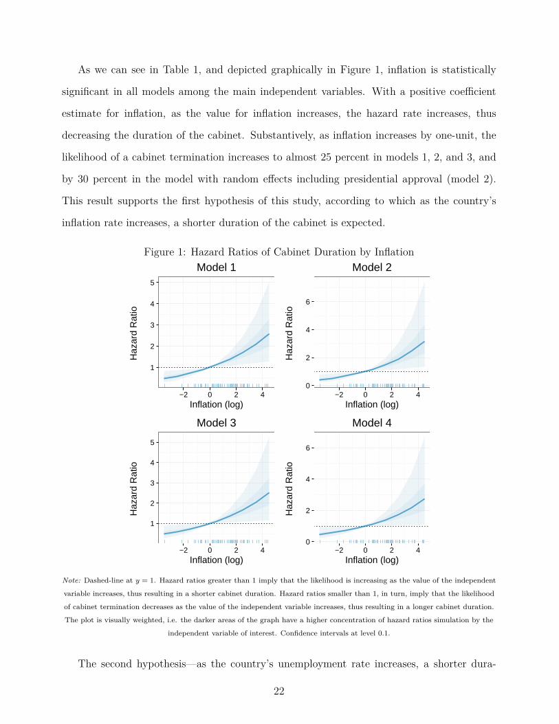
As we can see in Table 1, and depicted graphically in Figure 1, inflation is statistically

significant in all models among the main independent variables. With a positive coefficient

estimate for inflation, as the value for inflation increases, the hazard rate increases, thus

decreasing the duration of the cabinet. Substantively, as inflation increases by one-unit, the

likelihood of a cabinet termination increases to almost 25 percent in models 1, 2, and 3, and

by 30 percent in the model with random effects including presidential approval (model 2).

This result supports the first hypothesis of this study, according to which as the country’s

inflation rate increases, a shorter duration of the cabinet is expected.

Figure 1: Hazard Ratios of Cabinet Duration by Inflation

1

2

3

4

5

−2 0 2 4Inflation (log)

Haz

ard

Rat

io

Model 1

0

2

4

6

−2 0 2 4Inflation (log)

Haz

ard

Rat

io

Model 2

1

2

3

4

5

−2 0 2 4Inflation (log)

Haz

ard

Rat

io

Model 3

0

2

4

6

−2 0 2 4Inflation (log)

Haz

ard

Rat

io

Model 4

Note: Dashed-line at y = 1. Hazard ratios greater than 1 imply that the likelihood is increasing as the value of the independent

variable increases, thus resulting in a shorter cabinet duration. Hazard ratios smaller than 1, in turn, imply that the likelihood

of cabinet termination decreases as the value of the independent variable increases, thus resulting in a longer cabinet duration.

The plot is visually weighted, i.e. the darker areas of the graph have a higher concentration of hazard ratios simulation by the

independent variable of interest. Confidence intervals at level 0.1.

The second hypothesis—as the country’s unemployment rate increases, a shorter dura-

22

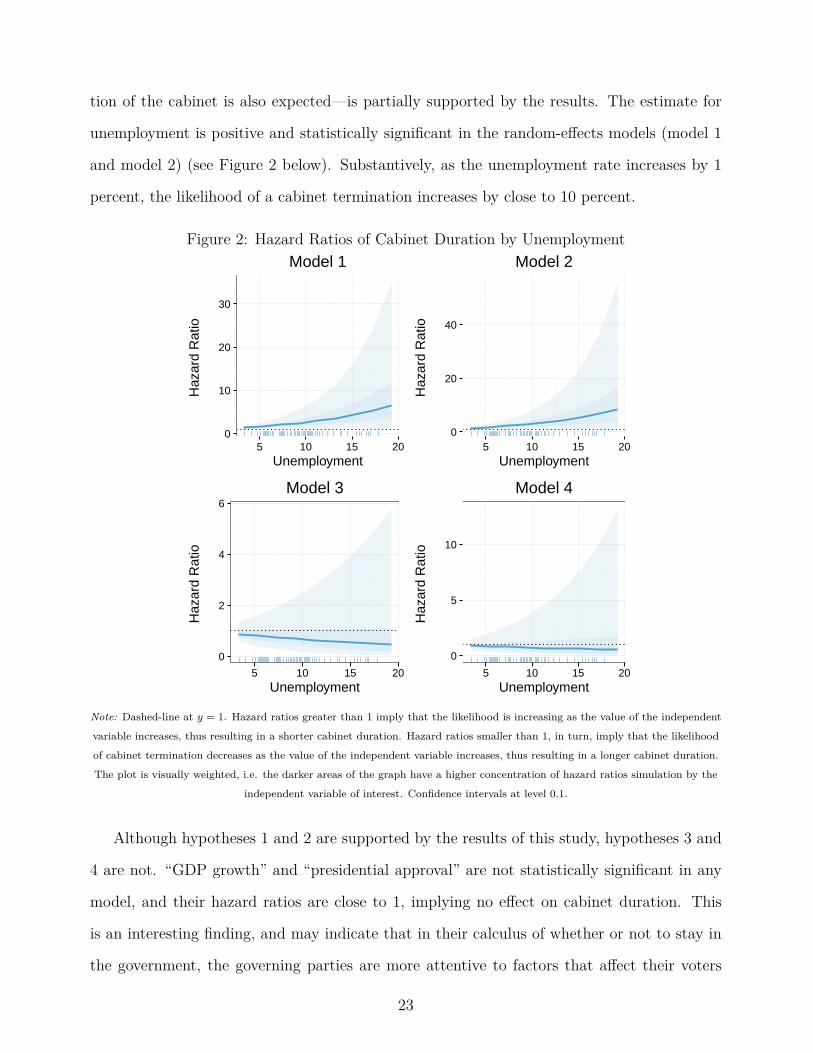
tion of the cabinet is also expected—is partially supported by the results. The estimate for

unemployment is positive and statistically significant in the random-effects models (model 1

and model 2) (see Figure 2 below). Substantively, as the unemployment rate increases by 1

percent, the likelihood of a cabinet termination increases by close to 10 percent.

Figure 2: Hazard Ratios of Cabinet Duration by Unemployment

0

10

20

30

5 10 15 20Unemployment

Haz

ard

Rat

io

Model 1

0

20

40

5 10 15 20Unemployment

Haz

ard

Rat

io

Model 2

0

2

4

6

5 10 15 20Unemployment

Haz

ard

Rat

io

Model 3

0

5

10

5 10 15 20Unemployment

Haz

ard

Rat

io

Model 4

Note: Dashed-line at y = 1. Hazard ratios greater than 1 imply that the likelihood is increasing as the value of the independent

variable increases, thus resulting in a shorter cabinet duration. Hazard ratios smaller than 1, in turn, imply that the likelihood

of cabinet termination decreases as the value of the independent variable increases, thus resulting in a longer cabinet duration.

The plot is visually weighted, i.e. the darker areas of the graph have a higher concentration of hazard ratios simulation by the

independent variable of interest. Confidence intervals at level 0.1.

Although hypotheses 1 and 2 are supported by the results of this study, hypotheses 3 and

4 are not. “GDP growth” and “presidential approval” are not statistically significant in any

model, and their hazard ratios are close to 1, implying no effect on cabinet duration. This

is an interesting finding, and may indicate that in their calculus of whether or not to stay in

the government, the governing parties are more attentive to factors that affect their voters

23

directly, such as inflation and unemployment.

Regarding the control variables, it is noteworthy that the results do not support the

“tyranny of the electoral calendar” hypothesis. An increase in the independent variable

“cycle”—meaning that a new election is closer—results in a estimate not statistically sig-

nificant and in the opposite direction expected by the “tyranny of the electoral calendar”

hypothesis. According to the theory proposed in this study, these results go in favor of the

expected outcomes. That is, when the model specified includes factors such as economic

indicators, no relationship between the elapsing of the president’s term and the cabinet ter-

mination is found.

The estimates for the variables “size of the Coalition” and “effective number of parties

(ENP)” are the only statistically significant control variables. It indicates that both the

fragmentation within the coalition and the fragmentation of the party systems are—along

with inflation and unemployment—strong predictors of cabinet termination. As the coalition

increases by one more party, the likelihood of a cabinet termination increases by almost 50

percent (statistically significant at level 0.05 in model 3, and at level 0.1 in model 4). The

estimate for ENP, in turn, is significant at and below level 0.05 in all models. A one-unit

increase in ENP increases the likelihood of a cabinet termination by almost 40 percent in

models 1 and 2, and by a little more than 50 percent in fixed-effect models 3 and 4.

These results show that the effects of the fragmentation of the coalition and of the frag-

mentation of the party system are stronger than the effects of inflation and unemployment on

cabinet duration. This reveals the importance of also considering institutional structures in

presidential systems—related to the fact that these structures can change the incentives for

the coalition formation. Nevertheless, the results for the economic indicators—inflation and

unemployment—reveal that the termination of coalition follows a logic that fits a rational be-

havior of the coalition’s members. When the government is successful in controlling inflation

and unemployment, cabinet termination becomes less likely.

24

6 Conclusions

In this study, I aimed to fill a major gap in the theoretical explanation of coalition termination

in presidential democracies by suggesting an answer to the question: Whether and under what

conditions are cabinet terminations more likely to happen in presidential systems? I proposed

a theoretical framework in which I adapt elements from the literature on cabinet survival in

parliamentary systems to the context of presidential systems. Considering that presidents

have some exclusive powers to form and reshuffle cabinets, I suggested that the termination of

a cabinet in presidential systems depends on contextual factors such as economic conditions—

inflation, unemployment, and economic growth—and the approval ratings of the president.

The results of this study partially support the hypotheses tested. Among the main inde-

pendent variables, inflation and unemployment rates were found to have an effect on cabinet

breakdown. As the country’s inflation and unemployment rates increase, the duration of the

cabinet decreases. Nevertheless, the effect of unemployment was found only for the random-

effects models, suggesting that this effect may actually be nested on countries’ specificities,

particularly for Brazil and Chile.9 The results also show that the fragmentation within the

cabinet and the party system are strong predictors of cabinet termination, revealing the im-

portance of also considering institutional structures in the analysis.

These results are similar to some findings regarding parliamentary systems. Warwick

(1992), for example, investigated the linkage between the trends of economic indicators and

government survival in 16 European parliamentary systems and found that both inflation and

unemployment are important explanatory factors for cabinet termination. Saalfeld (2008)

and Bergman (2015) also found that in parliamentary systems, cabinets facing unfavorable

macroeconomic situations have an increased risk of breakdown. Also, the polarization and

fractionalization of the party system were seen to be important factors on cabinet stability in

parliamentary studies (King, Alt, Burns, and Laver 1990; Laver and Schofield, 1990; Warwick,

1994; Diermeier and Stevenson, 1999). According to these studies, the more ideologically9See the results with country fixed-effects in Figure 7 in Appendix F.

25

diversified and fractionalized the party system, the higher the likelihood of early cabinet

terminations (Laver and Schofield, 1990).

In sum, whether in parliamentary systems or presidential systems, cabinet termination

has to be understood as the result of rational actors calculating the pros and cons of being

associated with the current government coalition. As shown in this study, in their calculation

of whether or not to stay in the government, governing parties are attentive to factors that

affect their voters directly, such as inflation and unemployment rates. Regarding the presi-

dential system context, the factors that make the termination of a coalition government more

likely are neither inherent structural problems nor the “tyranny of the electoral calendar.”

Although this study was restricted to Latin American democracies, the theory proposed

here is not restricted to these cases. The issue examined here has broader impacts beyond

Latin America, particularly in new presidential democracies outside the Americas, including

South Korea, the Philippines, and several countries in Africa. The availability of new data

will make it possible to test the theory proposed here in a broader comparative perspective.

As new data become available, other covariates that can affect cabinet termination but

could not be considered in this study can also enter into the analysis, such as the effects of

corruption and political scandals. Moreover, the results from this study raise new questions

that can be examined in future research. For example, why do some cabinets that are faced

with unfavorable economic and political conditions dissolve immediately, while other cabinets

do not? This is a potential research question for further studies on a topic that has only

recently begun to receive more attention from scholars of presidential systems.

26

References

Alemán, Eduardo, and George Tsebelis. 2011. “Political Parties and Government Coalitions

in the Americas.” Journal of Politics in Latin America 3 (1): 3–28.

Alt, James, and Gary King. 1994. “Transfers of Governmental Power: The Meaning of Time

Dependence.” Comparative Political Studies 27 (2): 190–210.

Altman, David. 2000a. “Coalition Formation and Survival under Multiparty Presidential

Democracies in Latin America: Between the Tyranny of the Electoral Calendar, the Irony

of Ideological Polarization, and Inertial Effects.” Paper presented at the Meeting of the Latin

American Studies Association, Hyatt Regency, Miami.

Altman, David. 2000b. “The Politics of Coalition Formation and Survival in Multiparty Pres-

idential Democracies: The Case of Uruguay, 1989-1999.” Party Politics 6 (3): 259–283.

Amorim Neto, Octavio. 2000a. “Gabinetes Presidenciais, Ciclos Eleitorais e Disciplina Leg-

islativa no Brasil.” Dados 43 (3): 1–25.

Amorim Neto, Octavio. 2000b. “Presidential Cabinets, Electoral Cycles, and Coalition Disci-

pline in Brazil.” Working Paper: 1–29.

Amorim Neto, Octavio. 2006a. Presidencialismo e Governabilidade nas Américas. Rio de

Janeiro: FGV; Konrad Adenauer Stiffung.

Amorim Neto, Octavio. 2006b. “The Presidential Calculus: Executive Policy Making and

Cabinet Formation in the Americas.” Comparative Political Studies 39 (4): 415–440.

Araújo, Victor. 2016. “Mecanismos de Alinhamento de Preferências em Governos Multipar-

tidários: Controle de Políticas Públicas no Presidencialismo Brasileiro.” Dissertation de-

fended at University of São Paulo (PhD Degree in Political Science), São Paulo.

27

Araújo, Victor, Andrea Freitas and Marcelo Vieira. 2015. “Parties and Control Over Pol-

icy: The Presidential Logic of Government Formation.” Paper presented at 73rd Annual

Conference of the Midwest Political Science Association. Chicago.

Bergman, Torbjörn, Svante Ersson, and Johan Hellström. 2015. “Government Formation and

Breakdown in Western and Central Eastern Europe.” Comparative European Politics 13 (3):

345–375.

Box-Steffensmeier, Janet, and Bradford Jones. 2004. Event History Modeling: A Guide for

Social Scientists. Cambridge: Cambridge University Press.

Carlin, Ryan, Cecilia Martínez-Gallardo, and Jonathan Hartlyn. 2012. “Executive Approval

Dynamics under Alternative Democratic Regime Types.” In Institutions and Democracy:

Essays in Honor of Alfred Stepan, ed. Douglas Chalmers and Scott Mainwaring. South

Bend: University of Notre Dame Press.

CEBRAP. 2015. “Legislative Dataset of the Brazilian Center of Analysis and Planning (CE-

BRAP).” http://neci.fflch.usp.br/node/506.

Chasquetti, Daniel. 1999. “Compartiendo el Gobierno: Multipartidismo y Coaliciones en

Uruguay (1971-1997).” Revista Uruguaya de Ciencia Política 10: 25–46.

Chasquetti, Daniel. 2001. “Democracia, Multipartidismo y Coaliciones en América Latina:

Evaluando La Difícil Combinación.” In Tipos de Presidencialismo y Coaliciones Políticas

en América Latina, ed. Jorge Lanzaro. Buenos Aires: CLACSO - Consejo Latinoamericano

de Ciencias Sociales.

Cheibub, José Antonio. 2007. Presidentialism, Parliamentarism, and Democracy. Cambridge:

Cambridge University Press.

Cheibub, José Antonio, Adam Przeworski, and Sebastián Saiegh. 2004. “Government Coali-

tions and Legislative Success Under Presidentialism and Parliamentarism.” British Journal

of Political Science 34: 565–587.

28

Cheibub, José Antonio, and Fernando Limongi. 2002. “Democratic Institutions and Regime

Survival: Parliamentary and Presidential Democracies Reconsidered.” Annual Review of

Political Science 5: 151–179.

Cheibub, José Antonio, and Fernando Limongi. 2011. “From Conflict to Coordination: Per-

spectives on the Study of Executive-Legislative Relations.” Iberian-American Journal of

Legislative Studies 1 (1): 38–53.

Cheibub, José Antonio, Jennifer Gandhi, and James Vreeland. 2010. “Democracy and Dicta-

torship Revisited.” Public Choice 143 (1-2): 67–101.

Cheibub, José Antonio, Zachary Elkins, and Tom Ginsburg. 2014. “Beyond Presidentialism

and Parliamentarism.” British Journal of Political Science 44 (3): 284–312.

Collier, David, and Robert Adcock. 1999. “Democracy and Dichotomies: A Pragmatic Ap-

proach to Choices about Concepts.” Annual Review of Political Science 2: 537–565.

Coppedge, Michael. 1997. “A Classification of Latin American Politicla Parties.” Kellog Insti-

tute, Working Paper 244.

Cox, David. 1972. “Regression Models and Life Tables.” Journal of the Royal Statistical Society

34: 187–220.

Cox, David. 1975. “Partial Likelihood.” Biometrika 62: 269–276.

Cox, David, and David Oakes. 1984. Analysis of Survival Data. New York: Chapman and

Hall.

Deheza, Grace Ivana. 1998. “Gobiernos de Coalición en el Sistema Presidencial: América del

Sur.” In El Presidencialismo Renovado: Instituciones y Cambio Político en América Latina,

ed. Dieter Nohlen and Mario Fernández B. Caracas: Nueva Sociedad.

Diermeier, Daniel, and Randy Stevenson. 1999. “Cabinet Survival and Competing Risks.”

American Journal of Political Science 43 (4): 1051–1068.

29

Druckman, James, and Michael Thies. 2002. “The Importance of Concurrence: The Impact

of Bicameralism on Government Formation and Duration.” American Journal of Political

Science 46 (4): 760–771.

EAP. 2015. “The Executive Approval Project (EAP).” http://www.executiveapproval.org.

Falcó-Gimeno, Albert, and Indridi Indridason. 2013. “Uncertainty, Complexity, and Gamson’s

Law: Comparing Coalition Formation in Western Europe.” West European Politics 36 (1):

221–247.

Figueiredo, Argelina. 2007. “Government Coalitions in Brazilian Democracy.” Brazilian Polit-

ical Science Review 1 (2): 182–216.

Figueiredo, Argelina, Denise Salles, and Marcelo Vieira. 2009. “Political and Institutional

Determinants of the Executive’s Legislative Success in Latin America.” Brazilian Political

Science Review 3 (2): 155–171.

Figueiredo, Argelina, and Fernando Limongi. 1999. Executivo e Legislativo na Nova Ordem

Constitucional. Rio de Janeiro: FGV.

Figueiredo, Argelina, and Fernando Limongi. 2007. “Instituições Políticas e Governabilidade:

Desempenho do Governo e apoio Legislativo na Democracia Brasileira.” In A Democracia

Brasileira. Balanço e Perspectivas para o Século 21, ed. C. Melo and M. Sáez (Eds.). Belo

Horizonte: Editora UFMG.

Fisher, Lloyd, and Danyu Lin. 1999. “Time-Dependent Covariates in the Cox Proportional-

Hazards Regression Model.” Annual Review of Public Health 20: 145–157.

Freitas, Andrea. 2013. “O Presidencialismo da Coalizão.” Dissertation defended at University

of São Paulo (PhD Degree in Political Science), São Paulo.

Grofman, Bernard, and Peter van Roozendaal. 1994. “Toward a Theoretical Explanation of

Premature Cabinet Termination.” European Journal of Political Research 26 (2): 155–170.

30

Grofman, Bernard, and Peter van Roozendaal. 1997. “Modelling Cabinet Durability and Ter-

mination.” British Journal of Political Science 27 (03): 419–451.

Indridason, Indridi, and Christopher Kam. 2008. “Cabinet Reshuffles and Ministerial Drift.”

British Journal of Political Science 38 (621–656).

Jones, Mark. 1995. Electoral Laws and the Survival of Presidential Democracies. South Bend:

Notre Dame University Press.

King, Gary, James Alt, Nancy Burns, and Michael Laver. 1990. “A Unified Model of Cabinet

Dissolution in Parliamentary Democracies.” American Journal of Political Science 34 (3):

846–871.

Laakso, Helsinki M., and Irvine R. Taagepera. 1979. “Effective Number of Parties: A Measure

with Application to West Europe.” Comparative Political Studies 12: 3–27.

Lanzaro, Jorge, ed. 2001. Tipos de Presidencialismo y Coaliciones Políticas en América Latina.

Buenos Aires: CLACSO - Consejo Latinoamericano de Ciencias Sociales.

Laver, Michael, and Kenneth Shepsle. 1994. Cabinet Ministers and Parliamentary Govern-

ment. Cambridge: Cambridge University Press.

Laver, Michael, and Norman Schofield. 1990. Multiparty Government: The Politics of Coali-

tion in Europe. Ann Arbor: The University of Michigan Press.

Limongi, Fernando. 2003. “Formas de Governo, Leis Partidárias e Processo Decisório.” BIB-

Revista Brasileira de Informação Bibliográfica em Ciências Sociais 55: 7–40.

Linz, Juan. 1990. “The Perils of Presidentialism.” Journal of Democracy 1 (1): 51–69.

Linz, Juan. 1994. “Presidential or Parliamentary Democracy: Does It Make a Difference?”

In The Failure of Presidential Democracy: The Case of Latin America, ed. Juan Linz and

Arturo Valenzuela. Baltimore: Johns Hopkins University Press.

31

Lupia, Arthur, and Kaare Strøm. 1995. “Coalition Termination and the Strategic Timing of

Parliamentary Elections.” American Political Science Review 89 (3): 648–665.

Mainwaring, Scott. 1993. “Presidentialism, Multipartism and Democracy: The Difficult Com-

bination.” Comparative Political Studies 26 (2): 198–228.

Mainwaring, Scott, and Matthew Shugart. 1997. Presidentialism and Democracy in Latin

America. Cambridge: Cambridge University Press.

Martínez-Gallardo, Cecilia. 2012. “Out of the Cabinet: What Dries Defections From the

Government in Presidential Systems?” Comparative Political Studies 45 (1): 62–90.

Martínez-Gallardo, Cecilia. 2014. “Designing Cabinets: Presidential Politics and Ministerial

Instability.” Journal of Politics in Latin America 6 (2): 3–38.

Martinussen, Torben, and Thomas Scheike. 2006. Dynamic Regression Models for Survival

Data. New York: Springer.

Mayorga, René. 2001. “Presidencialismo Parlamentarizado y Gobiernos de Coalición en Bo-

livia.” In Tipos de Presidencialismo y Coaliciones Políticas en América Latina, ed. Jorge

Lanzaro. Buenos Aires: CLACSO - Consejo Latinoamericano de Ciencias Sociales.

Melo, Marcus André, and Carlos Pereira. 2013. Making Brazil Work: Checking the President

in a Multiparty System. New York: Palgrave Macmillan.

Montero, Mercedes García. 2009. Presidentes y Parlamentos: £Quién Controla la Actividad

Legislativa en América Latina? Montalbán: Centro de Investigaciones Sociológicas.

Narud, Hanne Marthe. 1995. “Coalition Termination in Norway: Models and Cases.” Scandi-

navian Political Studies 18 (1): 1–24.

Novaro, Marcos. 2001. “Presidentes, Equilibrios Institucionales y Coaliciones de Gobierno en

Argentina (1989-2000).” In Tipos de Presidencialismo y Coaliciones Políticas en América

32

Latina, ed. Jorge Lanzaro. Buenos Aires: CLACSO - Consejo Latinoamericano de Ciencias

Sociales.

Przeworski, Adam, Michael Alvarez, José Antonio Cheibub, and Fernando Limongi. 2000.

Democracy and Development: Political Institutions and Well-Being in the World, 1950-

1990. Cambridge: Cambridge University Press.

Robertson, John. 1983a. “Inflation, Unemployment, and Government Collapse: A Poisson

Application.” Comparative Political Studies 15 (4): 425–444.

Robertson, John. 1983b. “The Political Economy and the Durability of European Coalition

Cabinets: New Variations on a Game-Theoretic Perspective.” The Journal of Politics 45 (4):

932–957.

Robertson, John. 1984. “Toward a Political-Economic Accounting of the Endurance of Cabinet

Administrations: An Empirical Assessment of Eight European Democracies.” American

Journal of Political Science 28 (4): 693–709.

Saafeld, Thomas. 2008. “Institutions, Chance, and Choices: The Dynamics of Cabinet Sur-

vival.” In Cabinets and Coalition Bargaining: The Democratic Life Cycle in Western Eu-

rope, ed. Kaare Strøm, Wolfgang Müller, and Torbjörn Bergman. Oxford: Oxford University

Press.

Saez, Manuel Alcántara and Flavia Freidenberg, eds. 2001. Partidos Políticos de América

Latina. Salamanca: Ediciones Universidad.

Sanders, David, and Valentine Herman. 1977. “The Stability and Survival of Governments in

Western Democracies.” Acta Politica 12 (3): 346–377.

Schofield, Norman, and Michael Laver. 1985. “Bargaining Theory and Portfolio Payoffs in

European Coalition Governments, 1945-1983.” British Journal of Political Science 15 (2):

143–164.

33

Shugart, Matthew, and John Carey. 1992. Presidents and Assemblies: Constitutional Design

and Electoral Dynamics. Cambridge: Cambridge University Press.

Siavelis, Peter. 2000. The President and Congress in Post-Authoritarian Chile: Institutional

Constraints to Democratic Consolidation. University Park: Pennsylvania State University

Press.

Silva, Thiago. 2016. “Who Gets What? The Importance of Ministerial Budget in the Al-

location of Portfolios in Presidential Multiparty Systems.” Paper presented at the XXXIV

International Congress of the Latin American Studies Association, New York City, NY,

USA.

Stepan, Alfred, and Cindy Skach. 1993. “Constitutional Frameworks and Democratic Consol-

idation: Parliamentarianism versus Presidentialism.” World Politics 46 (1): 1–22.

Strøm, Kaare. 1984. “Minority Governments in Parliamentary Democracies: The Rationality

of Nonwinning Cabinet Solutions.” Comparative Political Studies 17 (2): 199–227.

Strøm, Kaare. 1988. “Contending Models of Cabinet Stability.” American Political Science

Review 82 (3): 738–754.

Strøm, Kaare. 1990. Minority Government and Majority Rule. Cambridge: Cambridge Uni-

versity Press.

Strøm, Kaare, Wolfgang Müller, and Torbjörn Bergman, ed. 2008. Cabinets and Coalition

Bargaining: The Democratic Life Cycle in Western Europe. Oxford: Oxford University

Press.

Taylor, Michael, and Valentine Herman. 1971. “Party Systems and Government Stability.”

American Political Science Review 65 (1): 28–37.

The World Bank. 2014. “World Bank Open Data: Economic Indicators.”

http://data.worldbank.org/indicator/NY.GDP.MKTP.KD.ZG.

34

Thomas, Laine, and Eric Reyes. 2014. “Tutorial: Survival Estimation for Cox Regression

Models with Time-Varying Coefficients Using SAS and R.” Journal of Statistical Software

61 (1): 1–23.

Warwick, Paul. 1992. “Economic Trends and Government Survival in West European Parlia-

mentary Democracies.” American Political Science Review 86 (4): 875–887.

Warwick, Paul. 1994. Government Survival in Parliamentary Democracies. Cambridge: Cam-

bridge University Press.

35

Appendix Material

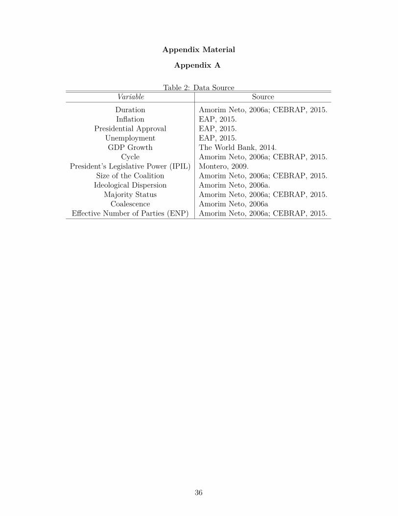
Appendix A

Table 2: Data SourceVariable SourceDuration Amorim Neto, 2006a; CEBRAP, 2015.Inflation EAP, 2015.

Presidential Approval EAP, 2015.Unemployment EAP, 2015.GDP Growth The World Bank, 2014.

Cycle Amorim Neto, 2006a; CEBRAP, 2015.President’s Legislative Power (IPIL) Montero, 2009.

Size of the Coalition Amorim Neto, 2006a; CEBRAP, 2015.Ideological Dispersion Amorim Neto, 2006a.

Majority Status Amorim Neto, 2006a; CEBRAP, 2015.Coalescence Amorim Neto, 2006a

Effective Number of Parties (ENP) Amorim Neto, 2006a; CEBRAP, 2015.

36

Appendix B

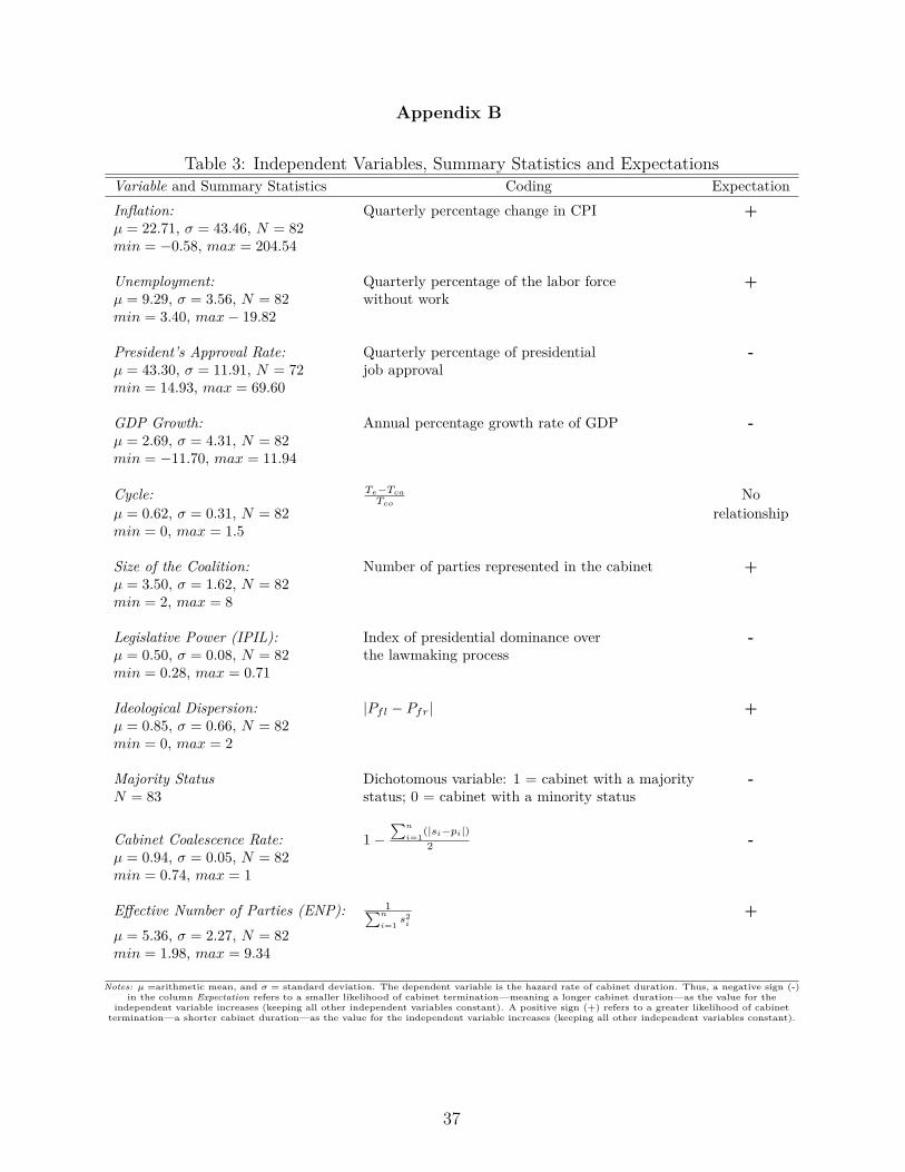
Table 3: Independent Variables, Summary Statistics and ExpectationsVariable and Summary Statistics Coding ExpectationInflation: Quarterly percentage change in CPI +µ = 22.71, σ = 43.46, N = 82min = −0.58, max = 204.54

Unemployment: Quarterly percentage of the labor force +µ = 9.29, σ = 3.56, N = 82 without workmin = 3.40, max− 19.82

President’s Approval Rate: Quarterly percentage of presidential -µ = 43.30, σ = 11.91, N = 72 job approvalmin = 14.93, max = 69.60

GDP Growth: Annual percentage growth rate of GDP -µ = 2.69, σ = 4.31, N = 82min = −11.70, max = 11.94

Cycle: Te−Tca

TcoNo

µ = 0.62, σ = 0.31, N = 82 relationshipmin = 0, max = 1.5

Size of the Coalition: Number of parties represented in the cabinet +µ = 3.50, σ = 1.62, N = 82min = 2, max = 8

Legislative Power (IPIL): Index of presidential dominance over -µ = 0.50, σ = 0.08, N = 82 the lawmaking processmin = 0.28, max = 0.71

Ideological Dispersion: |Pfl − Pfr| +µ = 0.85, σ = 0.66, N = 82min = 0, max = 2

Majority Status Dichotomous variable: 1 = cabinet with a majority -N = 83 status; 0 = cabinet with a minority status

Cabinet Coalescence Rate: 1−∑n

i=1(|si−pi|)2 -

µ = 0.94, σ = 0.05, N = 82min = 0.74, max = 1

Effective Number of Parties (ENP): 1∑n

i=1s2

i

+µ = 5.36, σ = 2.27, N = 82min = 1.98, max = 9.34

Notes: µ =arithmetic mean, and σ = standard deviation. The dependent variable is the hazard rate of cabinet duration. Thus, a negative sign (-)in the column Expectation refers to a smaller likelihood of cabinet termination—meaning a longer cabinet duration—as the value for the

independent variable increases (keeping all other independent variables constant). A positive sign (+) refers to a greater likelihood of cabinettermination—a shorter cabinet duration—as the value for the independent variable increases (keeping all other independent variables constant).

37

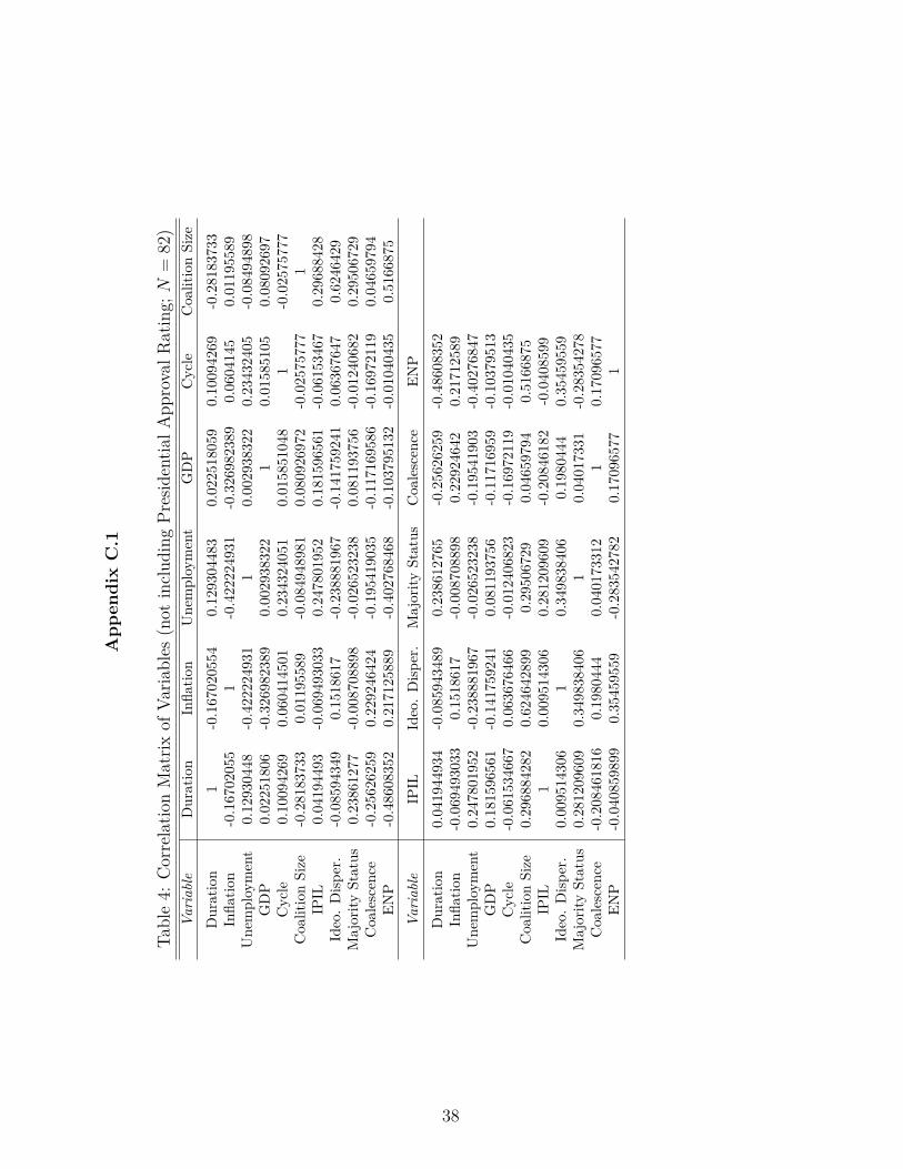
App

endi

xC

.1

Table4:

Correlatio

nMatrix

ofVa

riables

(not

includ

ingPr

esidentia

lApp

rovalR

ating;N

=82)

Variable

Duration

Infla

tion

Unemployment

GDP

Cycle

CoalitionSize

Duration

1-0.167020554

0.129304483

0.022518059

0.10094269

-0.28183733

Infla

tion

-0.16702055

1-0.422224931

-0.326982389

0.0604145

0.01195589

Unemployment

0.12930448

-0.422224931

10.002938322

0.23432405

-0.08494898

GDP

0.02251806

-0.326982389

0.002938322

10.01585105

0.08092697

Cycle

0.10094269

0.060414501

0.234324051

0.015851048

1-0.02575777

CoalitionSize

-0.28183733

0.01195589

-0.084948981

0.080926972

-0.02575777

1IP

IL0.04194493

-0.069493033

0.247801952

0.18159656

1-0.06153467

0.29688428

Ideo.Disp

er.

-0.08594349

0.1518617

-0.238881967

-0.141759241

0.06367647

0.6246429

Majority

Status

0.23861277

-0.008708898

-0.026523238

0.081193756

-0.01240682

0.29506729

Coalescence

-0.25626259

0.229246424

-0.195419035

-0.117169586

-0.16972119

0.04659794

ENP

-0.48608352

0.217125889

-0.402768468

-0.103795132

-0.01040435

0.5166875

Variable

IPIL

Ideo.Disp

er.

Majority

Status

Coalescence

ENP

Duration

0.041944934

-0.085943489

0.238612765

-0.25626259

-0.48608352

Infla

tion

-0.069493033

0.1518617

-0.008708898

0.22924642

0.21712589

Unemployment

0.247801952

-0.238881967

-0.026523238

-0.19541903

-0.40276847

GDP

0.181596561

-0.141759241

0.081193756

-0.11716959

-0.10379513

Cycle

-0.061534667

0.063676466

-0.012406823

-0.16972119

-0.01040435

CoalitionSize

0.296884282

0.624642899

0.29506729

0.04659794

0.5166875

IPIL

10.009514306

0.281209609

-0.20846182

-0.0408599

Ideo.Disp

er.

0.009514306

10.349838406

0.1980444

0.35459559

Majority

Status

0.281209609

0.349838406

10.04017331

-0.28354278

Coalescence

-0.208461816

0.1980444

0.040173312

10.17096577

ENP

-0.040859899

0.35459559

-0.283542782

0.17096577

1

38

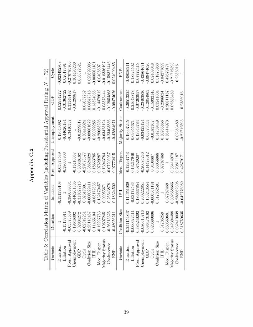
App

endi

xC

.2

Table5:

Correlatio

nMatrix

ofVa

riables

(includ

ingPr

esidentia

lApp

rovalR

ating;N

=72)

Variable

Duration

Infla

tion

Pres.App

roval

Unemployment

GDP

Cycle

Duration

1-0.151399108

-0.05373539

0.19646092

0.02934272

-0.023492808

Infla

tion

-0.15139911

1-0.38603803

-0.44626184

-0.31362722

0.02617391

Pres.App

roval

-0.05373539

-0.386038034

1-0.13410337

0.33348182

-0.2707857

66Unemployment

0.19646092

-0.446261836

-0.13410337

1-0.01299817

0.304493238

GDP

0.02934272

-0.313627218

0.33348182

-0.01299817

10.056372521

Cycle

-0.02349281

0.02617391

-0.27078577

0.30449324

0.05637252

1CoalitionSize

-0.25115487

-0.006022411

0.38524029

-0.08661672

0.08647316

0.020699096

IPIL

0.11465104

-0.03172536

0.18663785

0.20022285

0.15324055

-0.000561181

Ideo.Disp

er.

-0.12297753

0.132179457

0.07529287

-0.20085236

-0.14478612

0.0408607

Majority

Status

0.19607245

0.09955671

0.13943784

-0.03423124

0.05373444

-0.018336197

Coalescence

-0.26513325

0.25643878

-0.07203957

-0.23403836

-0.12054863

-0.159321446

ENP

-0.48056211

0.18324502

0.07772415

-0.42864671

-0.09474026

0.024090485

Variable

CoalitionSize

IPIL

Ideo.Disp

er.

Majority

Status

Coalescence

ENP

Duration

-0.251154867

0.114651039

-0.12297753

0.19607245

-0.26513325

-0.48056211

Infla

tion

-0.006022411

-0.03172536

0.13217946

0.09955671

0.25643878

0.18324502

Pres.App

roval

0.385240292

0.186637854

0.07529287

0.13943784

-0.07203957

0.07772415

Unemployment

-0.086616716

0.200222851

-0.20085236

-0.03423124

-0.23403836

-0.42864671

GDP

0.086473162

0.153240554

-0.14478612

0.05373444

-0.12054863

-0.09474026

Cycle

0.020699096

-0.000561181

0.0408607

-0.0183362

-0.15932145

0.02409048

CoalitionSize

10.317352591

0.66056968

0.34239449

0.03241004

0.51875963

IPIL

0.31735259

10.07787469

0.30265866

-0.2386624

-0.04277699

Ideo.Disp

er.

0.660569681

0.07787469

10.36414973

0.20811187

0.42679171

Majority

Status

0.342394488

0.302658665

0.36414973

10.02383489

-0.21712593

Coalescence

0.032410039

-0.238662398

0.20811187

0.02383489

10.2356916

ENP

0.518759635

-0.042776989

0.42679171

-0.21712593

0.2356916

1

39

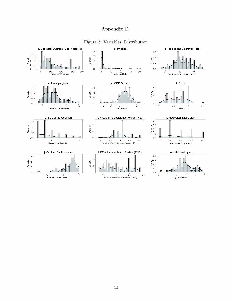
Appendix D

Figure 3: Variables’ Distribution

40

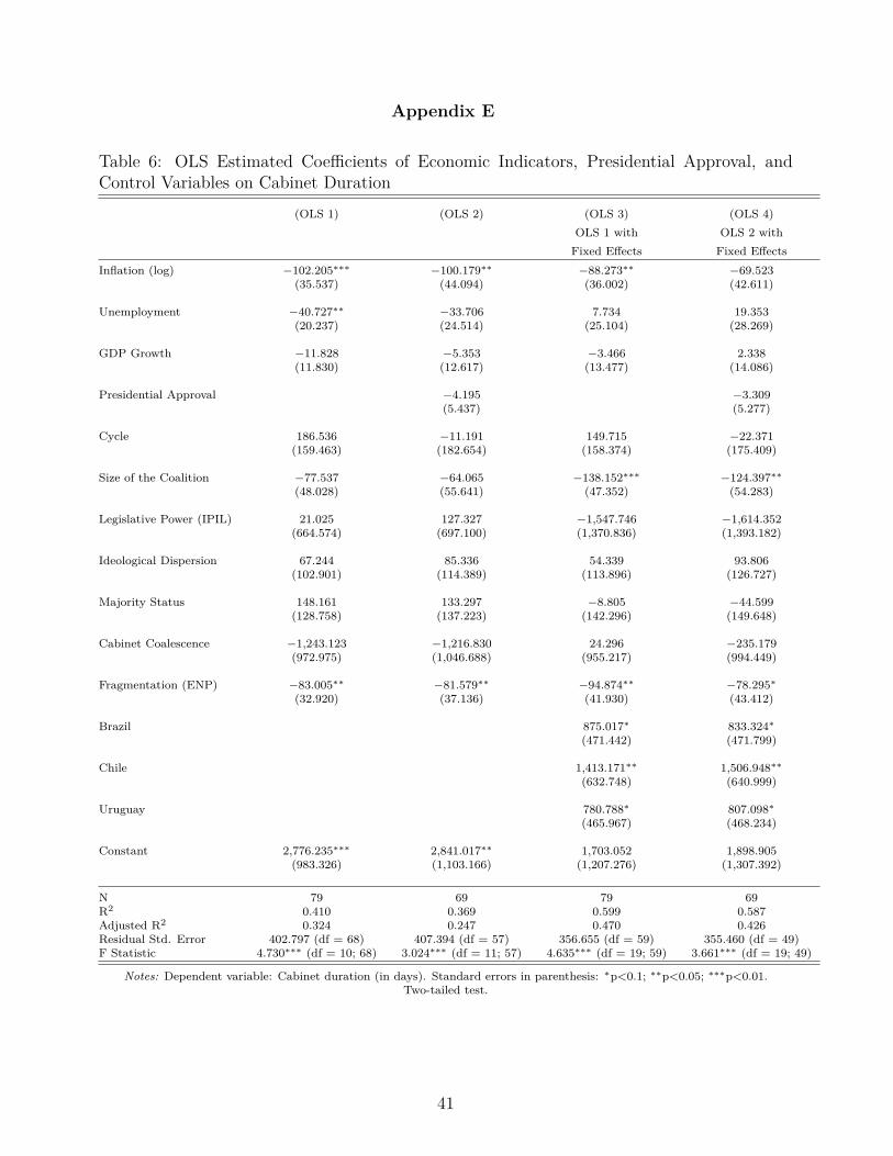
Appendix E

Table 6: OLS Estimated Coefficients of Economic Indicators, Presidential Approval, andControl Variables on Cabinet Duration

(OLS 1) (OLS 2) (OLS 3) (OLS 4)OLS 1 with OLS 2 withFixed Effects Fixed Effects

Inflation (log) −102.205∗∗∗ −100.179∗∗ −88.273∗∗ −69.523(35.537) (44.094) (36.002) (42.611)

Unemployment −40.727∗∗ −33.706 7.734 19.353(20.237) (24.514) (25.104) (28.269)

GDP Growth −11.828 −5.353 −3.466 2.338(11.830) (12.617) (13.477) (14.086)

Presidential Approval −4.195 −3.309(5.437) (5.277)

Cycle 186.536 −11.191 149.715 −22.371(159.463) (182.654) (158.374) (175.409)

Size of the Coalition −77.537 −64.065 −138.152∗∗∗ −124.397∗∗

(48.028) (55.641) (47.352) (54.283)

Legislative Power (IPIL) 21.025 127.327 −1,547.746 −1,614.352(664.574) (697.100) (1,370.836) (1,393.182)

Ideological Dispersion 67.244 85.336 54.339 93.806(102.901) (114.389) (113.896) (126.727)

Majority Status 148.161 133.297 −8.805 −44.599(128.758) (137.223) (142.296) (149.648)

Cabinet Coalescence −1,243.123 −1,216.830 24.296 −235.179(972.975) (1,046.688) (955.217) (994.449)

Fragmentation (ENP) −83.005∗∗ −81.579∗∗ −94.874∗∗ −78.295∗

(32.920) (37.136) (41.930) (43.412)

Brazil 875.017∗ 833.324∗

(471.442) (471.799)

Chile 1,413.171∗∗ 1,506.948∗∗

(632.748) (640.999)

Uruguay 780.788∗ 807.098∗

(465.967) (468.234)

Constant 2,776.235∗∗∗ 2,841.017∗∗ 1,703.052 1,898.905(983.326) (1,103.166) (1,207.276) (1,307.392)

N 79 69 79 69R2 0.410 0.369 0.599 0.587Adjusted R2 0.324 0.247 0.470 0.426Residual Std. Error 402.797 (df = 68) 407.394 (df = 57) 356.655 (df = 59) 355.460 (df = 49)F Statistic 4.730∗∗∗ (df = 10; 68) 3.024∗∗∗ (df = 11; 57) 4.635∗∗∗ (df = 19; 59) 3.661∗∗∗ (df = 19; 49)

Notes: Dependent variable: Cabinet duration (in days). Standard errors in parenthesis: ∗p<0.1; ∗∗p<0.05; ∗∗∗p<0.01.Two-tailed test.

41

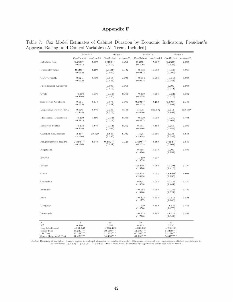
Appendix F

Table 7: Cox Model Estimates of Cabinet Duration by Economic Indicators, President’sApproval Rating, and Control Variables (All Terms Included)

Model 1 Model 2 Model 3 Model 4Coefficient exp(coeff.) Coefficient exp(coeff.) Coefficient exp(coeff.) Coefficient exp(coeff.)

Inflation (log) 0.208∗∗ 1.231 0.263∗∗ 1.301 0.204∗ 1.227 0.222∗ 1.249(0.091) (0.119) (0.106) (0.127)

Unemployment 0.096∗ 1.101 0.108∗ 1.114 −0.038 0.963 −0.033 0.967(0.052) (0.064) (0.081) (0.099)

GDP Growth 0.021 1.021 0.015 1.016 −0.004 0.996 −0.015 0.985(0.032) (0.033) (0.043) (0.044)

Presidential Approval 0.006 1.006 0.009 1.009(0.015) (0.018)

Cycle −0.306 0.736 −0.184 0.832 −0.379 0.685 −0.125 0.882(0.410) (0.456) (0.425) (0.475)

Size of the Coalition 0.111 1.117 0.078 1.081 0.393∗∗ 1.482 0.373∗ 1.452(0.123) (0.141) (0.162) (0.194)

Legislative Power (IPIL) 0.626 1.870 0.784 2.189 5.505 245.894 5.311 202.539(1.444) (1.579) (4.640) (4.894)

Ideological Dispersion −0.109 0.896 −0.128 0.880 −0.070 0.933 −0.250 0.778(0.281) (0.318) (0.417) (0.468)

Majority Status −0.138 0.871 −0.135 0.874 0.151 1.163 0.256 1.292(0.334) (0.362) (0.416) (0.442)

Cabinet Coalescence 2.317 10.140 1.843 6.314 1.525 4.596 1.733 5.656(2.150) (2.299) (2.994) (3.032)

Fragmentation (ENP) 0.316∗∗∗ 1.371 0.352∗∗∗ 1.422 0.450∗∗∗ 1.568 0.412∗∗ 1.510(0.106) (0.121) (0.162) (0.164)

Argentina 0.515 1.673 0.209 1.233(1.896) (1.951)

Bolivia −1.450 0.235(1.353)

Brazil −2.344∗ 0.096 −2.298 0.101(1.376) (1.413)

Chile −3.373∗ 0.034 −3.638∗ 0.026(2.029) (2.135)

Colombia 0.024 1.025 −0.333 0.717(1.353) (1.444)

Ecuador −0.014 0.986 −0.286 0.751(1.310) (1.324)

Peru −0.423 0.655 −0.515 0.598(1.177) (1.186)

Uruguay −1.179 0.308 −1.536 0.215(1.450) (1.470)

Venezuela −0.923 0.397 −1.314 0.269(1.718) (1.841)

N 79 69 79 69R2 0.360 0.367 0.533 0.530Log Likelihood −251.667 −210.429 −239.188 −200.121Wald Test 34.230∗∗∗ 30.560∗∗∗ 51.600∗∗∗ 44.280∗∗∗

LR Test 35.248∗∗∗ 31.522∗∗∗ 60.205∗∗∗ 52.139∗∗∗

Score (Logrank) Test 37.429∗∗∗ 34.496∗∗∗ 61.750∗∗∗ 54.677∗∗∗

Notes: Dependent variable: Hazard ratios of cabinet duration = exp(coefficients). Standard errors of the (non-exponentiate) coefficients inparenthesis: ∗p<0.1; ∗∗p<0.05; ∗∗∗p<0.01. Two-tailed test. Statistically significant estimates are in bold.

42

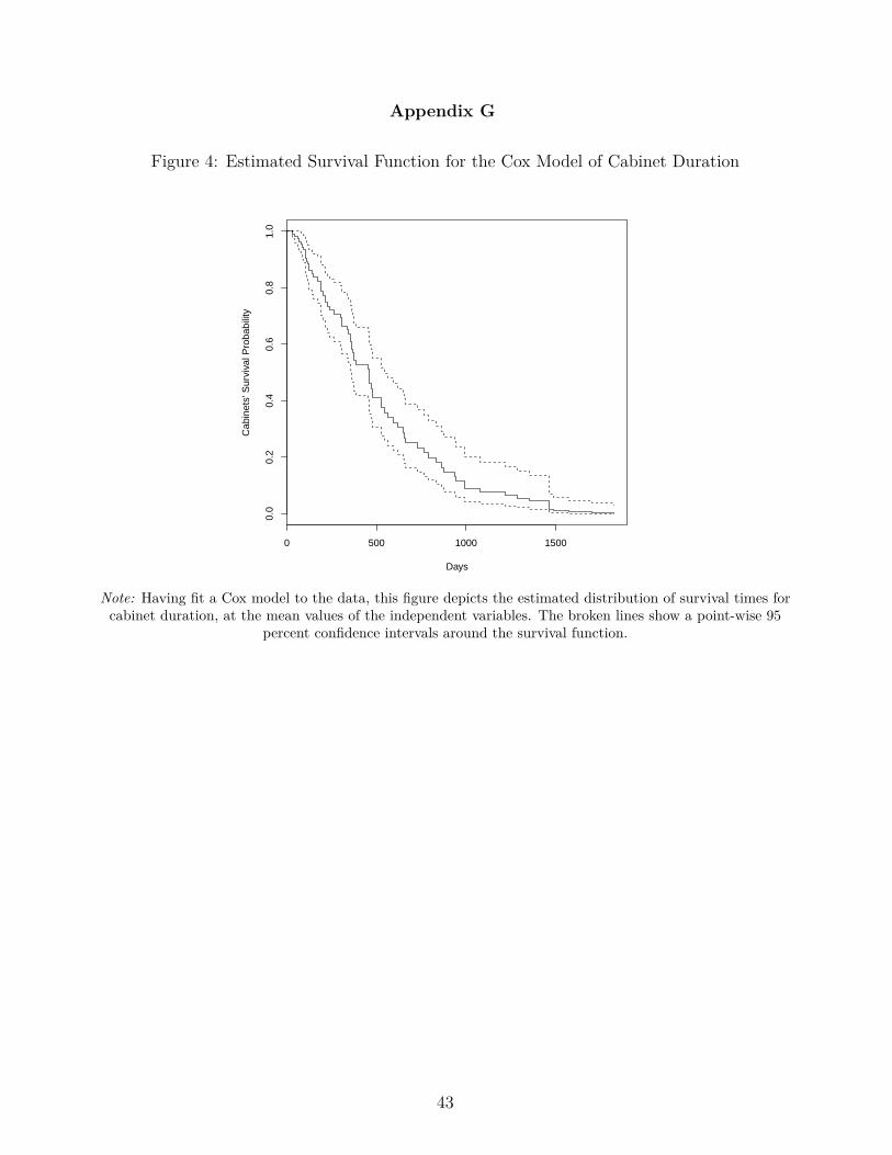
Appendix G

Figure 4: Estimated Survival Function for the Cox Model of Cabinet Duration

0 500 1000 1500

0.0

0.2

0.4

0.6

0.8

1.0

Days

Cab

inet

s' S

urvi

val P

roba

bilit

y

Note: Having fit a Cox model to the data, this figure depicts the estimated distribution of survival times forcabinet duration, at the mean values of the independent variables. The broken lines show a point-wise 95

percent confidence intervals around the survival function.

43

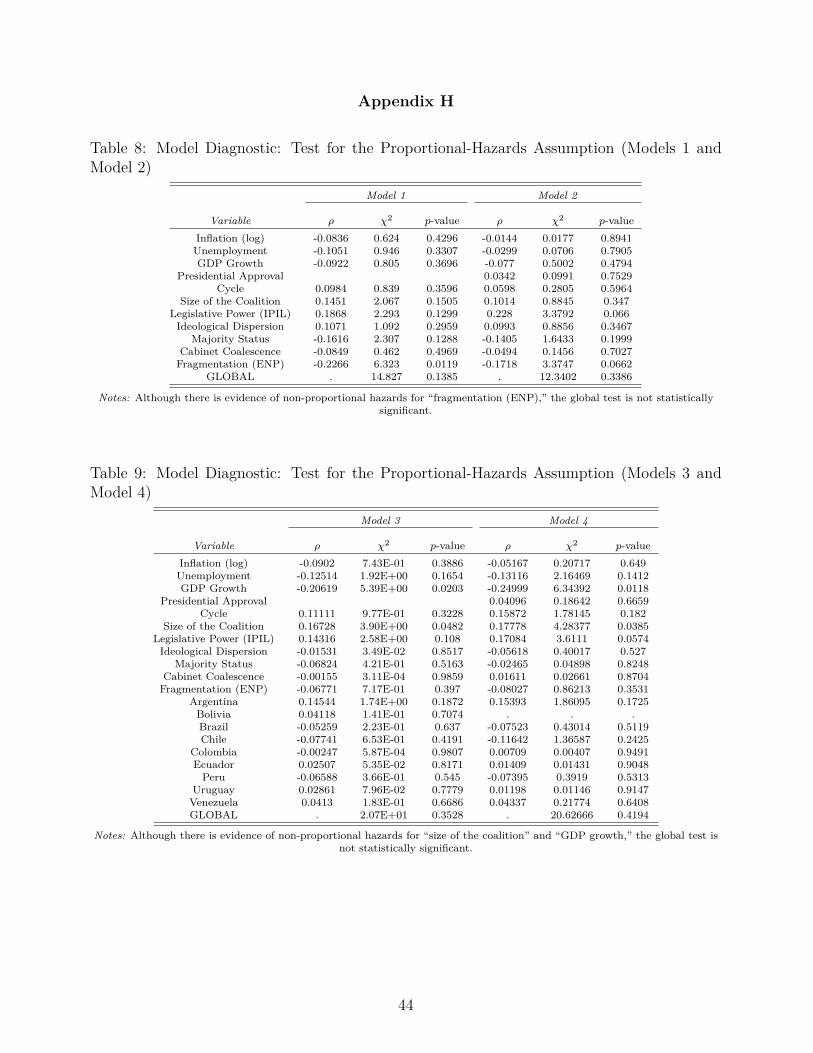
Appendix H

Table 8: Model Diagnostic: Test for the Proportional-Hazards Assumption (Models 1 andModel 2)

Model 1 Model 2

Variable ρ χ2 p-value ρ χ2 p-valueInflation (log) -0.0836 0.624 0.4296 -0.0144 0.0177 0.8941Unemployment -0.1051 0.946 0.3307 -0.0299 0.0706 0.7905GDP Growth -0.0922 0.805 0.3696 -0.077 0.5002 0.4794

Presidential Approval 0.0342 0.0991 0.7529Cycle 0.0984 0.839 0.3596 0.0598 0.2805 0.5964

Size of the Coalition 0.1451 2.067 0.1505 0.1014 0.8845 0.347Legislative Power (IPIL) 0.1868 2.293 0.1299 0.228 3.3792 0.066Ideological Dispersion 0.1071 1.092 0.2959 0.0993 0.8856 0.3467

Majority Status -0.1616 2.307 0.1288 -0.1405 1.6433 0.1999Cabinet Coalescence -0.0849 0.462 0.4969 -0.0494 0.1456 0.7027Fragmentation (ENP) -0.2266 6.323 0.0119 -0.1718 3.3747 0.0662

GLOBAL . 14.827 0.1385 . 12.3402 0.3386

Notes: Although there is evidence of non-proportional hazards for “fragmentation (ENP),” the global test is not statisticallysignificant.

Table 9: Model Diagnostic: Test for the Proportional-Hazards Assumption (Models 3 andModel 4)

Model 3 Model 4

Variable ρ χ2 p-value ρ χ2 p-valueInflation (log) -0.0902 7.43E-01 0.3886 -0.05167 0.20717 0.649Unemployment -0.12514 1.92E+00 0.1654 -0.13116 2.16469 0.1412GDP Growth -0.20619 5.39E+00 0.0203 -0.24999 6.34392 0.0118

Presidential Approval 0.04096 0.18642 0.6659Cycle 0.11111 9.77E-01 0.3228 0.15872 1.78145 0.182

Size of the Coalition 0.16728 3.90E+00 0.0482 0.17778 4.28377 0.0385Legislative Power (IPIL) 0.14316 2.58E+00 0.108 0.17084 3.6111 0.0574Ideological Dispersion -0.01531 3.49E-02 0.8517 -0.05618 0.40017 0.527

Majority Status -0.06824 4.21E-01 0.5163 -0.02465 0.04898 0.8248Cabinet Coalescence -0.00155 3.11E-04 0.9859 0.01611 0.02661 0.8704Fragmentation (ENP) -0.06771 7.17E-01 0.397 -0.08027 0.86213 0.3531

Argentina 0.14544 1.74E+00 0.1872 0.15393 1.86095 0.1725Bolivia 0.04118 1.41E-01 0.7074 . . .Brazil -0.05259 2.23E-01 0.637 -0.07523 0.43014 0.5119Chile -0.07741 6.53E-01 0.4191 -0.11642 1.36587 0.2425

Colombia -0.00247 5.87E-04 0.9807 0.00709 0.00407 0.9491Ecuador 0.02507 5.35E-02 0.8171 0.01409 0.01431 0.9048Peru -0.06588 3.66E-01 0.545 -0.07395 0.3919 0.5313

Uruguay 0.02861 7.96E-02 0.7779 0.01198 0.01146 0.9147Venezuela 0.0413 1.83E-01 0.6686 0.04337 0.21774 0.6408GLOBAL . 2.07E+01 0.3528 . 20.62666 0.4194

Notes: Although there is evidence of non-proportional hazards for “size of the coalition” and “GDP growth,” the global test isnot statistically significant.

44

Appendix I.1

Figure 5: Model Diagnostics: Influential Observations in Model 1

●●

●●●

●●

●

●●●

●

●●●●

●

●

●

●

●

●●

●●

●

●

●●●

●

●

●●

●●

●

●

●

●

●

●

●

●●

●

●

●

●

●

●

●

●

●

●

●

●

●

●●

●●●

●

●

●

●

●

●

●

●●

●

●

●●

●●

●

0 20 40 60 80

−0.

05−

0.03

−0.

010.

01DfBETA for Inflation(log)

Index

Infla

tion(

log)

●●●

●●

●

●

●

●

●

●●

●

●

●●

●

●

●

●

●

●

●

●

●

●●

●

●

●

●

●

●

●

●

●

●●

●

●

●●

●●

●

●

●●

●

●●

●

●

●

●

●

●

●

●●●

●

●

●

●

●

●

●

●

●

●●●

●

●●

●●

●

0 20 40 60 80

−0.

010

0.00

00.

010

DfBETA for Unemployment

IndexU

nem

ploy

men

t

●●

●

●●

●

●

●

●●

●

●

●

●

●●

●

●●●

●

●

●

●

●

●●

●

●●

●●

●●

●

●

●

●

●

●

●

●

●

●

●●

●

●

●

●

●

●

●

●

●

●

●

●

●●

●

●●

●

●

●

●

●

●

●●

●

●

●●

●●

●

●

0 20 40 60 80

−0.

04−

0.02

0.00

0.02

DfBETA for ENP

Index

EN

P

Note: Dashed-line at y = 0. This figure depicts the index plots produced by specifying the argumenttype = dfbeta to residuals in order to produce a matrix of estimated changes in the regression coefficientsupon deleting each observation in turn (the plots are only for the independent variables with statisticallysignificant estimates). Comparing the magnitudes of the largest dfbeta values to the regression coefficients

suggests that none of the observations is significantly influential individually.

45

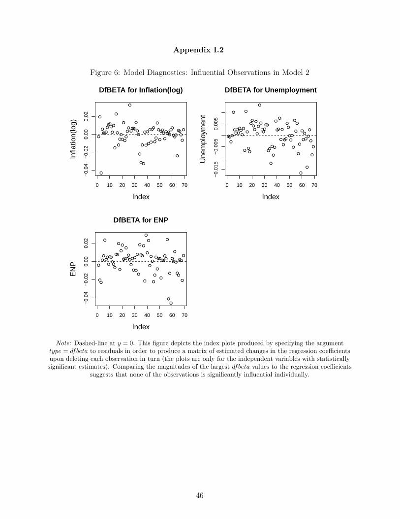
Appendix I.2

Figure 6: Model Diagnostics: Influential Observations in Model 2

●

●

●

●●●●

●●●

●

●

●

●

●

●

●

●

●

●

●

●●

●●

●

●●●●

●

●●

●

●

●

●

●

●

●

●

●

●

●●

●●

●

●

●

●●●

●

●●●●

●●

●●●

●

●●●

●

●

0 10 20 30 40 50 60 70

−0.

04−

0.02

0.00

0.02

DfBETA for Inflation(log)

Index

Infla

tion(

log)

●●

●

●

●

●●●●

●●

●

●

●

●

●

●●

●●

●●

●

●

●

●

●

●●●

●●

●●

●

●

●

●

●

●●

●

●

●

●

●●

●

●

●

●

●

●

●

●

●

●

●

●

●

●

●

●

●

●

●

●

●

●

0 10 20 30 40 50 60 70

−0.

015

−0.

005

0.00

5

DfBETA for Unemployment

IndexU

nem

ploy

men

t

●

●●

●

●

●

●●

●

●●

●●●

●●

●

●

●

●

●●

●

●●

●

●

●

●

●

●

●

●

●

●●

●

●

●

●

●

●

●

●

●

●

●

●

●●

●

●●

●●

●

●

●

●

●●

●

●

●●

●●

●

●

0 10 20 30 40 50 60 70

−0.

04−

0.02

0.00

0.02

DfBETA for ENP

Index

EN

P

Note: Dashed-line at y = 0. This figure depicts the index plots produced by specifying the argumenttype = dfbeta to residuals in order to produce a matrix of estimated changes in the regression coefficientsupon deleting each observation in turn (the plots are only for the independent variables with statisticallysignificant estimates). Comparing the magnitudes of the largest dfbeta values to the regression coefficients

suggests that none of the observations is significantly influential individually.

46

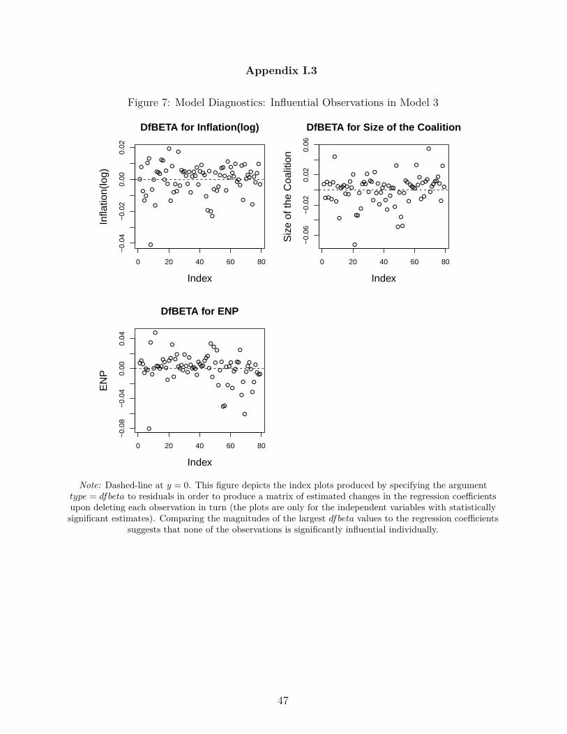
Appendix I.3

Figure 7: Model Diagnostics: Influential Observations in Model 3

●

●

●

●●

●●

●

●

●

●

●●●

●●

●

●

●

●

●

●

●

●

●

●

●

●●●●

●

●

●

●●●

●

●

●

●

●●

●

●

●

●●

●

●

●●

●

●●

●

●

●

●

●

●●

●

●●

●

●

●

●

●●●

●

●

●

●

●

●

●

0 20 40 60 80

−0.

04−

0.02

0.00

0.02

DfBETA for Inflation(log)

Index

Infla

tion(

log)

●

●

●

●

●

●

●

●

●

●

●

●●●

●

●

●

●

●

●

●

●●

●

●

●●●

●

●

●●

●

●

●

●

●

●●●

●

●

●

●

●●

●

●

●

●

●

●

●

●●

●

●●●●

●

●

●

●

●

●

●●

●

●●●●●

●

●

●

●

●

0 20 40 60 80

−0.

06−

0.02

0.02

0.06

DfBETA for Size of the Coalition

IndexS

ize

of th

e C

oalit

ion

●●●

●●●

●

●

●

●

●

●●●●

●●

●

●

●●

●

●

●●

●●●●

●

●

●

●

●●●●

●

●●●●

●●●

●

●

●

●

●

●

●

●

●

●●

●

●

●●

●

●●

●●

●

●

●

●

●

●●

●

●

●

●

●●●

0 20 40 60 80

−0.

08−

0.04

0.00

0.04

DfBETA for ENP

Index

EN

P

Note: Dashed-line at y = 0. This figure depicts the index plots produced by specifying the argumenttype = dfbeta to residuals in order to produce a matrix of estimated changes in the regression coefficientsupon deleting each observation in turn (the plots are only for the independent variables with statisticallysignificant estimates). Comparing the magnitudes of the largest dfbeta values to the regression coefficients

suggests that none of the observations is significantly influential individually.

47

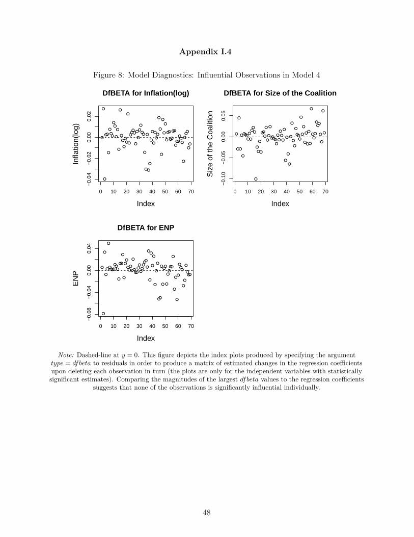
Appendix I.4

Figure 8: Model Diagnostics: Influential Observations in Model 4

●

●

●

●●

●

●

●●

●●

●

●

●

●

●

●

●

●●

●

●

●●●●

●

●

●

●

●

●●

●

●

●

●

●

●

●

●

●

●●

●

●

●

●

●

●

●

●●

●●

●●

●●●

●●●

●

●

●●

●●

0 10 20 30 40 50 60 70

−0.

04−

0.02

0.00

0.02

DfBETA for Inflation(log)

Index

Infla

tion(

log)

●

●

●

●

●

●

●●●●

●

●

●●

●

●

●

●

●

●

●●

●

●

●

●

●

●●●●

●

●

●

●

●

●

●

●

●

●

●

●

●

●

●

●

●●●

●

●

●

●

●

●

●

●

●

●●

●

●●●

●

●

●

●

0 10 20 30 40 50 60 70

−0.

10−

0.05

0.00

0.05

DfBETA for Size of the Coalition

IndexS

ize

of th

e C

oalit

ion

●

●

●

●

●

●

●●●●

●●●

●

●●

●

●

●●

●●●

●

●

●●●

●●

●●●●●

●

●

●

●

●

●

●

●

●

●●

●

●

●●

●

●●

●●

●

●

●

●

●

●●●

●

●

●

●●●

0 10 20 30 40 50 60 70

−0.

08−

0.04

0.00

0.04

DfBETA for ENP

Index

EN

P

Note: Dashed-line at y = 0. This figure depicts the index plots produced by specifying the argumenttype = dfbeta to residuals in order to produce a matrix of estimated changes in the regression coefficientsupon deleting each observation in turn (the plots are only for the independent variables with statisticallysignificant estimates). Comparing the magnitudes of the largest dfbeta values to the regression coefficients

suggests that none of the observations is significantly influential individually.

48

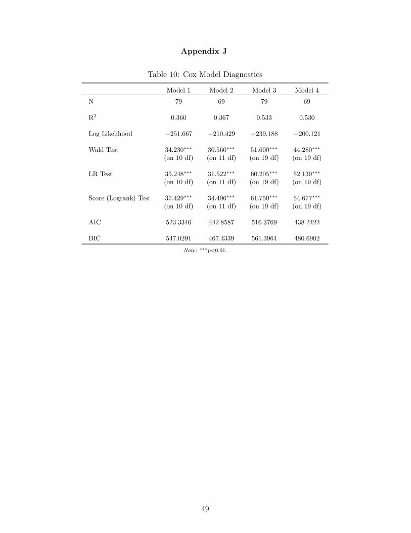
Appendix J

Table 10: Cox Model Diagnostics

Model 1 Model 2 Model 3 Model 4N 79 69 79 69

R2 0.360 0.367 0.533 0.530

Log Likelihood −251.667 −210.429 −239.188 −200.121

Wald Test 34.230∗∗∗ 30.560∗∗∗ 51.600∗∗∗ 44.280∗∗∗(on 10 df) (on 11 df) (on 19 df) (on 19 df)

LR Test 35.248∗∗∗ 31.522∗∗∗ 60.205∗∗∗ 52.139∗∗∗(on 10 df) (on 11 df) (on 19 df) (on 19 df)

Score (Logrank) Test 37.429∗∗∗ 34.496∗∗∗ 61.750∗∗∗ 54.677∗∗∗(on 10 df) (on 11 df) (on 19 df) (on 19 df)

AIC 523.3346 442.8587 516.3769 438.2422

BIC 547.0291 467.4339 561.3964 480.6902

Note: ∗∗∗p<0.01.

49