How many patients

do I need for my study?

Realistic Sample Size

Estimates for Clinical Trials

Sample Size Estimation1. General considerations

2. Continuous response variable– Parallel group comparisons

• Comparison of response after a specified period of follow-up• Comparison of changes from baseline

– Crossover study

3. Success/failure response variable– Impact of non-compliance, lag– Realistic estimates of control event rate (Pc) and event rate

pattern– Use of epidemiological data to obtain realistic estimates of

experimental group event rate (Pe)

4. Time to event designs and variable follow-up

Useful References

• Lachin JM, Cont Clin Trials, 2:93-113, 1981 (a general overview)

• Shih J, Cont Clin Trials, 16:395-407, 1995 (time to event studies with dropouts, dropins, and lag issues) – see size program on biostatistics network

• Farrington CP and Manning G, Stat Med, 9:1447-1454, 1990 (sample size for equivalence trials)

• Whitehead J, Stat Med, 12:2257-2271, 1993 (sample size for ordinal outcomes)

• Donner A, Amer J Epid, 114:906-914, 1981 (sample size for cluster randomized trials)

Key Points• Sample size should be specified in advance (often it is not)

• Sample size estimation requires collaboration and some time to do it right (not solely a statistical exercise)

• Often sample size is based on uncertain assumptions (estimates should consider a range of values for key parameters and the impact on power for small deviations in final assumptions should be considered)

• Parameters that do not involve the treatment difference (e.g., SD) on which sample size was based should be evaluated by protocol leaders (who are blinded to treatment differences) during the trial

• It pays to be conservative; however, ultimate size and duration of a study involves compromises, e.g., power, costs, timeliness.

Some Evidence that Sample Size is Not Considered Carefully: A Survey of 71

“Negative” Trials(Freiman et al., NEJM, 1978)

• Authors stated “no difference”• P-value > 0.10 (2-sided)• Success/failure endpoint• Expected number of events >5 in control and

experimental groups• Using the stated Type I error and control group event

rate, power was determined corresponding to:

– 25% difference between groups– 50% difference between groups

0-9 10-19 20-29 30-39 40-49 50-59 60-69 70-79 80-89 90-990

5

10

15

20

25

Power (1 - ß)

5.63%

25% Reduction

Frequency Distribution of Power Estimates for 71 “Negative” Trials

References: Frieman et al, NEJM 1978.

0-9 10-19 20-29 30-39 40-49 50-59 60-69 70-79 80-89 90-990

5

10

15

20

25

Power (1 - ß)

29.58%

Frequency Distribution of Power Estimates for 71 “Negative” Trials

50% Reduction

References: Frieman et al, NEJM 1978.

Implications of Review by Frieman et al.

• Many investigations do not estimate sample size in advance

• Many studies should never have been initiated; some were stopped too soon

• “Non-significant” difference does not mean there is not an important difference

• Design estimates (in Methods) are important to interpret study findings

• Confidence intervals should be used to summarize treatment differences

Studies with Power to Detect 25% and 50% Differences

6 6

6

6l

l

l

l

0

5

10

15

20

25

30

35

40

45

50

Per

cen

t o

f S

tud

ies

wit

h a

t L

east

80%

Po

wer

6 25% Differencel 50% Difference

1975 1980 1985 1990

Moher et al, JAMA , 272:122-124,1994

These Results Emphasize the Importance of Understanding that the Size of P-Value

Depends on:

• Magnitude of difference (strength of association); and

• Sample size

“Absence of evidence is not evidence of absence”, Altman and Bland, BMJ 1995; 311:485.

Steps in Planning a Study

1) Specify the precise research question

2) Define target population

3) Assess feasibility of studying question (compute sample size)

4) Decide how to recruit study participants, e.g., single center, multi-center, and make sure you have back-up plans

Beginning: A Protocol Stating Null and Alternative Hypotheses Along with Significance Level and

PowerNull hypothesis (HO)

Hypothesis of no difference or no association

Alternative hypothesis (HA)Hypothesis that there is a specified difference (Δ)

No direction specified (2-tailed)A direction specified (1-tailed)

Significance Level (): Type I Error

The probability of rejecting H0 given that H0 is true

Power = (1 - ): ( = Type II Error)

Power is the probability of rejecting H0 when the true difference is Δ

End: Test of Significance According to Protocol

Statistically Significant?

Yes No

RejectHO

Do not rejectHO

Sampling variationis an unlikely

explanation for thediscrepancy

Sampling variationis a likely

explanation for thediscrepancy

Normal Distribution

If Z is large (lies in yellow area), we assume difference in means is unlikely to have come from a distribution with mean zero.

Continuous Outcome Example

Observations: Many people have stage 1 (mild) hypertension (SBP 140-159 or DBP 90-99 mmHg)

For most, treatment is life-long

Many drugs which lower BP produce undesirable symptoms and metabolic effects (new drugs are

needed)

Research Can new drug T adequately control BP for patients Question: with mild hypertension?

Objective: To compare new drug T with diuretic treatment for lowering diastolic blood pressure (DBP)

Parallel Group Design Comparing Average Diastolic BP (DBP) After One Year

Hypothesis HO: DBP after one year of treatment with new drug T equals the DBP for patients given a diuretic (control)

HA: DBP after one year is different for patients given new drug T compared to diuretic

treatment (difference is 4 mmHg or more)

Study Population: Those with mild

hypertension

Drug T DBP at year 1

Diuretic DBP at year 1

Parallel Group Design Comparing Average Difference (Year 1 – Baseline) in DBP.

Hypothesis HO: DBP change from baseline after one year of treatment with new Drug T equals the DBP change from baseline after one year for patients given a diuretic (control)

HA: DBP change from baseline after one year of treatment with new Drug T is different

than the DBP change from baseline after one year for patients given a diuretic (control) treatment (difference is 4 mmHg or more)

Study Population: Those with mild

hypertension

Drug T Change in

DBP(Year 1 – Baseline)

DiureticChange in DBP

(Year 1 – Baseline)

Why Δ= 4 mmHg? An importantdifference on a population-wide basis

Clinical trials (Lancet 1990;335:827-38)

• 14 randomized trials; 36,908 participants

• 5-6 mmHg DBP difference (treatment vs. control)

• 28% reduction in fatal/non-fatal CVD

Observational studies (Lancet 2002;360:1903-13)

• 58 studies; 958,074 participants

• 5 mm Hg lower DBP among those 40-59 years

• 41% (30%) lower risk of death from stroke (CHD)

Considerations in Specifying Treatments Effect (Delta)

• Smallest difference of clinical significance/interest

• Stage of research

• Realistic and plausible estimates based on:– previous research

– expected non-compliance and switchover rates

– consideration of type of participants to be studied

• Resources (compromise)

Delta is a difference that is important NOT to miss if present.

Principal Determinants of Sample Size

• Size of difference considered important (Delta)

• Type I error () or significance level

• Type II error (), or power (1- )

• Variability of response/frequency of event

Constants

Sample Size for Two Groups: Equal Allocation

General Formula

2 x Variability x [Constant (,)]2

Delta2

N PerGroup

=

Delta = Δ = clinically relevant and plausible treatment difference

Sample Size Formula Derivation: One Sample Situation

;H

H

trueis H if 1)( Prob

and

trueis H if )( Prob

:satisfy tohas size Sample

:A

:o

A

o

o

o o

ZZ

ZZ

Sample Size Derivation (cont.)

2

211

2

1

21

A21

21 o

)(N

Nfor solve and :Note

N(0,1)

Prob

Hunder 1 0

Prob

sided)-(2 0.05For

96.1 ifHReject

0

ZZ

ZZ

Z

NZ

N

X

-Z

N

X

ZZN

XZ

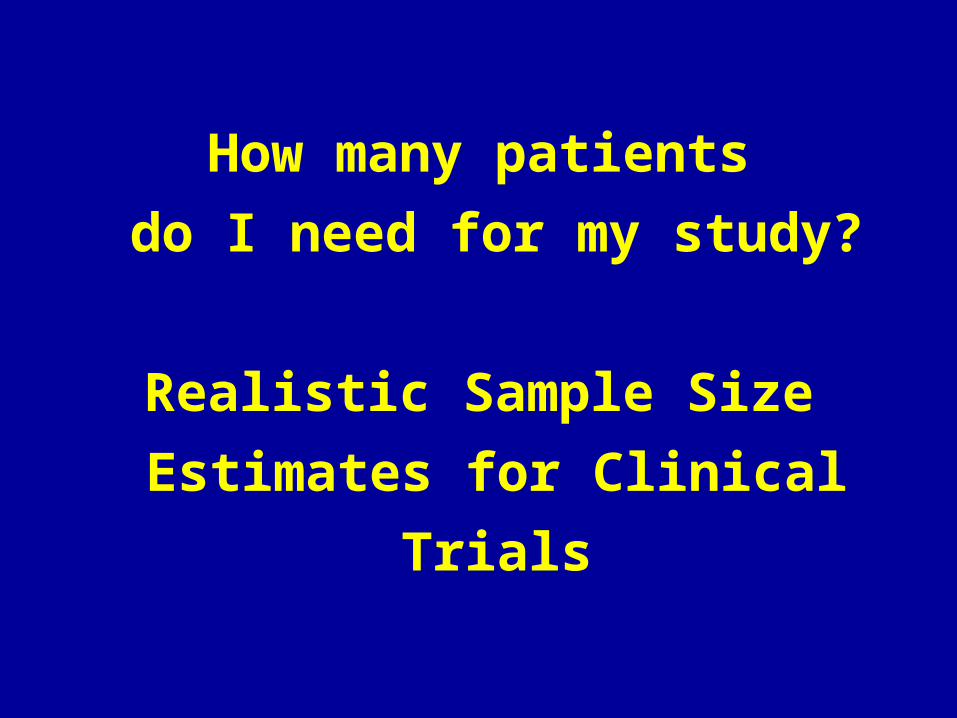
Weighing the Errors

Type 2 error: Sponsor’s concern

Type 1 error: Regulator’s Concern

0.05 (1.96) 0.80 (0.84) 7.84

0.90 (1.28) 10.50

0.95 (1.645) 13.00

0.01 (2.575) 0.80 (0.84) 11.67

0.90 (1.28) 14.86

0.95 (1.645) 17.81

Typical Values for (Z1-/2 + Z1- )2 Which Is Numerator of Sample Size

Type I Error ()or

Significance Level (Z1-/2)2-sided test

Power (1 - )(Z1-) (Z1-/2 + Z1-)2

Example

Hypertension Study

HO 1 2 1 2: = ; - = 0HA 1 2 1 2: ≠ ; - = 4 mmHg

HO HA

0 4 mmHg

Usually formulated in terms of change from baseline (e.g., Ho = D1 - D2 = 0)

Another Derivation

2

22

222

21

2

2

22

0

under 1Prob

2

under Prob

2

0

ZZN

ZZN

NZ

NZ

dd

HZZ

N

dZ

HZZ

Nnn

N

dZ

A

O

Solve for N using these2 equations and by noting

that Δ = sum of 2 partsfrom the previous figure .

Sources of Variability of BP Measurements

Ref: Rose GA. Standardization of Observers in Blood Pressure Measurement. Lancet 1965;1:673-4.

Variability ofblood pressurereadings

True variations in arterial pressure

Known factors

Unknown factors

Recent physical activityEmotional statePosition of subject and armRoom temperature and season of year

Measurementerrors

Instrument

Observer

Inaccuracy of sphygmomanometer

Cuff width and length

Chiefly affectingthe mean pressureestimate

Distorting the frequency distribution curve (and sometimes affecting the mean)

Mental concentrationHearing acuityConfusion of auditory and visualInterpretation of soundsRates of inflation and deflationReading of moving column

Terminal digit preference

Prejudice, e.g., excess of readings at 120/80

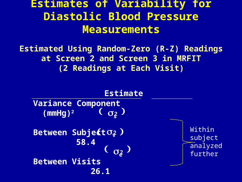
Estimates of Variability for Diastolic Blood Pressure Measurements (MRFIT)

Estimated Using Random-Zero (R-Z) Readings

EstimateVariance Component (mmHg)2

Between Subject 58.4

Within Subjects 36.3

s2

e2

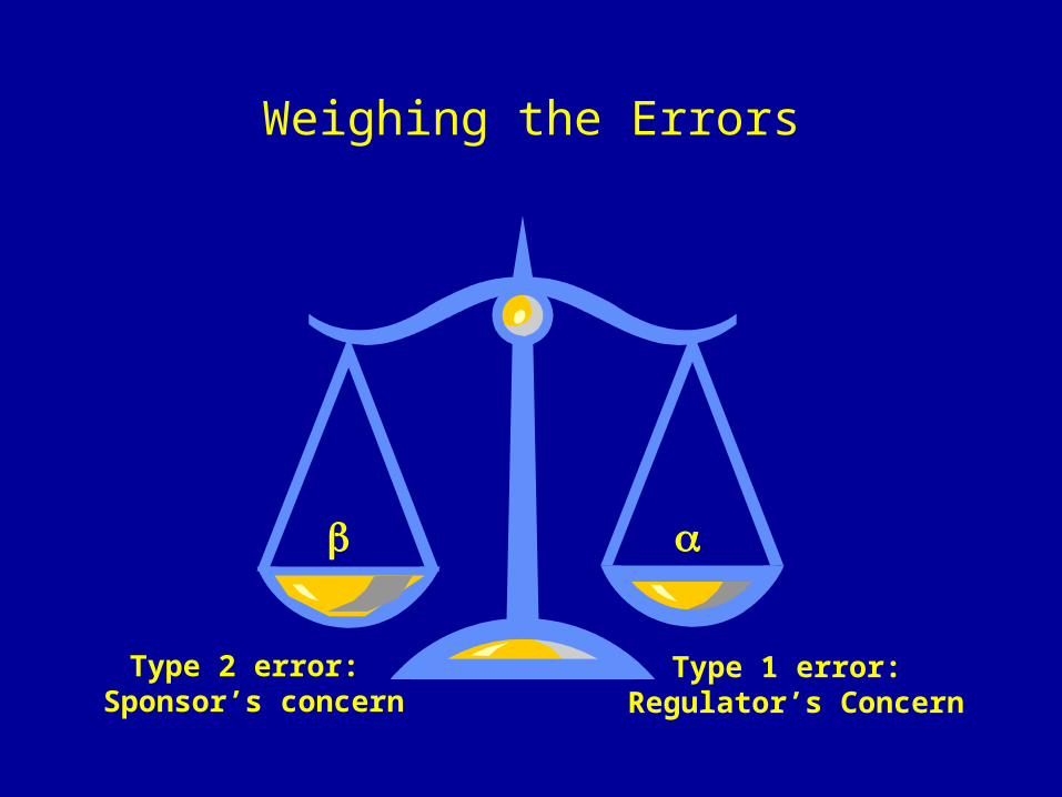
Estimates of Variability for Diastolic Blood Pressure Measurements

Estimated Using Random-Zero (R-Z) Readingsat Screen 2 and Screen 3 in MRFIT

(2 Readings at Each Visit)

EstimateVariance Component (mmHg)2

Between Subject 58.4

Between Visits 26.1

Between Readings 10.2

s2

v2

e2

Within subjectanalyzed further

Consequences on Sample Size of Using Multiple Readings for Defining Diastolic BP

=0.05, 1-=0.90Inter-subject variability=58.4 (mmHg)2

No. of No. ofvisits readings/visit ∆ = 8 ∆ = 4

1 1 31 124

1 2 30 118

2 1 25 100

2 2 24 97

Between visit variability = 26.1 (mmHg)2

Within visit variability = 10.2 (mmHg)2

N per Group

Parallel Group Design Comparing Average DBP After One Year.

Hypothesis HO: DBP after one year of treatment with new Drug T equals the DBP for

patients given a diuretic (control)

HA: DBP after one year is different for patients given new Drug T compared to diuretic

treatment (difference is 4 mmHg or more)

Study Population: Those with mild

hypertension

Drug T DBP at year 1

Diuretic DBP at year 1

Parallel Group StudiesComparing Average DBP After One Year

1 measure, 1 visit (a=0.05, b= .10)

1253.124

4

5.10)7.94(2=n=n

zz2

=n=n=n

4;:H

=:H

2CT

2

2

-1

2-1

2

CT

TCTA

CTO

C

3207.31

8

5.10)7.94(2=n=n

zz2

=n=n=n

8;:H

=:H

2CT

2

2

-1

2-1

2

CT

TCTA

CTO

C

s2=58.4 + 26.1+10.2=94.7

D=4 mmHg D=8 mmHg

Parallel Group Design Comparing Average Difference (Year 1 – Baseline) in DBP.

Hypothesis HO: DBP change from baseline after one year of treatment with new Drug T equals the DBP change from baseline after one year for patients given a diuretic (control) HA: DBP change from baseline after one year of

treatment with new Drug T is different than the DBP change from baseline after one year for patients given a diuretic (control) treatment (difference is 4 mmHg or more)

(2-Tailed)

Study Population: Those with mild

hypertension

Drug T Change in DBP

(Year 1 – Baseline)

DiureticChange in DBP

(Year 1 – Baseline)

Sample Size for Two Groups: Equal Allocation

General Formula

2 x Variability x [Constant (,)]2

Delta2

N PerGroup

=

Delta = Δ = clinically relevant and plausible treatment difference

Estimate of Variability for Change Outcome

• Prior studies (For MRFIT, SD of DBP change after 12 months = 9.0 mmHg [baseline is one visit, 2 readings; follow-up is one visit, 2 readings]. For comparison, SD of 12 month DBP is 9.5 mmHg)

• Use correlation (ρ) of repeat readings for participants to estimate e

2. (For MRFIT, correlation of DBP at baseline

and 12 months is 0.55; note that SD (diff) can be written as

2σT2 (1-ρ) = 2σe

2 = 2(81)(1-0.55) = 72.9 (SD of change ≈ 8.5 mmHg)

• Estimate of SD change using analysis of covariance (regression of change on baseline) (For MRFIT, SD = 7.9 mmHg)

2

22

222

22

222

22

2

22

2

21

122

2

e

es

ees

es

sesBF

tttBF

tyy

tyyBF

BFBBF

es

F

B

yy

so

yy

ppyyc

yyyVaryrVyy

y

y

BF

BF

)())(2()-Var(

,

)(2=)- Var(and

if

)(ov

)cov()()(a=)- Var(

tmeasuremen up-follow

tmeasuremen baseline Let

2

F

2t

Study Population: Those with mild

hypertension

Drug T Washout Period Diuretic

Diuretic Washout Period Drug T

Crossover Group Design Comparing Average Difference (Diuretic – Drug T) in DBP

Hypothesis HO: Average of paired differences for the two treatment sequences differences is zero.

HA: Average is 4 mmHg or more)

Crossover Study Design

1 2 Diff.

I y1 y2 dl

II y1 y2 dll

Period

Var(dl) = 2 e2

Var(dll) = 2 e2

=∆ = TT - TC = E dl + dll

2

– –Dl + Dll

2

With parallel group comparison we had:

or equivalently:

With crossover we have:

HO = TT – TC = 0

HO : mT = mC or HO : DT = DC where

Dl + Dll

2HO = = 0

DT and DC refer to the difference between

follow-up and baseline levels of outcome

Variance forSample Size Formula:

222 224

1

4

1

2

eee

IIIIII dd

ddVar

][

)var()var(

Substitution intoSample Size Formula Gives:

n| = n|| = number randomly allocated to each sequence - I (AB) or II (BA).

This follows because the variance of the pooled treatment difference across the 2 sequences is ¼ (22

e + 22 e)

2

2

-1

2-1

2e

IIIc

zzn=n=n

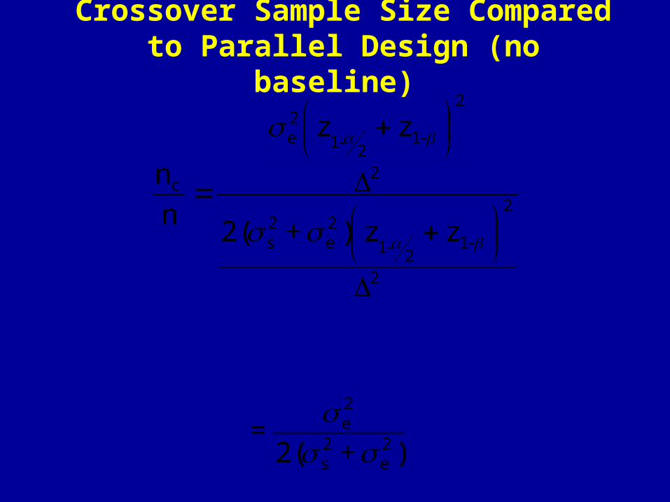
Crossover Sample Size Compared to Parallel Design (no baseline)

)+2(=

zz)+2(

zz

n

n

2e

2s

2e

-12-1

2e

2s

-12-1

2e

c

2

2

2

2

Crossover Sample Size Compared to Parallel Design (no baseline)

But the crossover design will require twice the number of measurements. So, if ρ= 0 then number of measurements are equal, but sample size for crossover is ½.

2

1

12

1

n)(n

+= since

)+2(n

n

+=

c

2e

2s

2e

2e

2s

2ec

2e

2s

2s

Consider an Experimentwith Diastolic BP Response

Type 1 error = 0.05 (2-sided) and Power = 0.95

99=n ,n 5,=

design group parallel

for needed patients more times 5

0.19 = )..(

.

n

n

(mmHg) 36.3 =

(mmHg) 58.4 =

c

c

22e

22s

19

3364582

336

Examples

DBP (mmHg) 58 36 0.62 0.19

Cholesterol (mg/dl) 1200 400 0.75 0.125

Overnight urine 325 625 0.34 0.33excretion Na+(meq/8 hours)

2 overnights 325 312 0.51 0.24

7 overnights 325 90 0.78 0.11

s2 e2

nc

n

2e

2e

2e

III

2eBA

2e

2sBA

2+24

1

2

d+dVar

consider toneed wecrossoverwith

4=)d-Var(d

or )+2(=)y-Var(y

consider to

need webaseline with scomparison group parallelWith

crossover to

compared baseline uses whichdesign group

parallel for required patients more times 4

is or whatof Regardless

4

1=

)zz)((

)zz(

baseline) withn(parallel

)(crossovern

-12-1

-12-1

c

2

2

22

2

22

4

e

e

e

Sample size for = .05 (2-sided) and = .05

ParallelNumber/group 163 72 41 26(no baseline)

ParallelBaseline 80 36 20 12number/group(r=0.75)

Crossover(Number/seq.) = 0.00 82 36 21 13 = 0.25 62 27 15 10 = 0.50 41 18 10 7 = 0.75 20 9 5 3

0.8 1.00.4 0.6

Key Points

• Sample size should be specified in advance

• Sample size estimation requires collaboration

• Often sample size is based on uncertain assumptions, therefore estimates should consider a range of values for key parameters (i.e., investigate the impact on power if sample size and treatment effect is not achieved)

• Parameters on which sample size is based should be evaluated during the trial

• It pays to be conservative; however, ultimate size and duration of a study involves compromises, e.g., power, costs, timeliness.

Power

Prob (rej Ho | when HA is true) = 1-b

1-b = (rej Ho | m1-m2 = D)

= Prob x 1 - x 2 - 0

s 12

n1

+ s 22

n2

³ Z1 -a 2

m1 -m2 = D

+ x 1- x 2 - 0

s12

n1

+s 2

2

n2

£ -Z1-a 2

m1 -m2 = D

Assume s 12 = s 2

2 = s 2 and n1=n2 =n

A measure of how likely the study will detecta specific treatment difference (∆), if present.

Power (cont.)

1-b = Prob x 1 - x 2 - D

2s 2

n

³ Z1-a 2

+0-D

2s 2

n

m1-m2 = D

é

ë

ê ê ê ê ê

ù

û

ú ú ú ú ú

+ Prob x 1 - x 2 -D2s 2

n

£ -Z1-a 2

+ 0 -D2s 2

n

m1-m2 = D

é

ë

ê ê ê ê ê

ù

û

ú ú ú ú ú

=Prob Z ³ Z1-a 2

-D

2s 2

n

é

ë

ê ê ê ê ê

ù

û

ú ú ú ú ú

+

Prob Z £ -Z1-a 2

- D2s 2

n

Usually one of these probabilities will be very close to zero, depending on whether ∆ is positive or negative.

Power (cont.)

5752

961

21

21

21

221

. 0.01;=

. 0.05;=

Prob=

then 0, Prob 2nd then 0, > If

c

n

Sensitivity of Power to Variations in Other Sample Size Parameters

(Assume s2 = 100)

0.05 4 100 -0.87 0.81

0.01 4 100 -0.25 0.60

0.05 6 100 -2.28 0.99

0.01 6 100 -1.67 0.95

0.05 4 200 -2.04 0.98

0.01 4 200 -1.425 0.92

a ∆ n Zc Power

Unequal Sample Sizes

%.k For

/)(2 1:k versus 1:1 for size sample Relative

)(Nc

)allocation 1:(kkNc Ν

)(.Nc

SE(diff)

)allocation 1:(2Nc Ν

T

T

5124542

41

11

51

2

11

2

2

22

2

2

/. k

k

ZZk

ZZ

NN cc

Another Formulation: Unequal Allocation

Comparison of means (Treatment C vs. E):

PC and PE= fraction of patients assigned control (C) and experimental treatment (E); PC+ PE = 1

Total N =

s 2 1P

C

+ 1P

E

æ

è ç ç

ö

ø÷ ÷ Z

1-a

2

+ Z1- b

æ

è ç ç

ö

ø÷ ÷

2

Δ2

Total Sample Size for Different Allocation Ratios

Allocation Ratio (E:C)

∆ (mm Hg) 1:1 2:1 3:1 1:2

4 250 280 332 280

8 64 70 84 70

0.90 β)-1(Power

test)sided-(2 05.

)Hg (mm 7.94 22

Sample sizes rounded up

Multiple Treatments and Unequal Allocation

Example: m experimental treatments and control; comparison of means

Problem: Find n which minimizes variance

mn-N

+n

=XXV

E(x)=

treatment

alexperiment each to response = X

treatment control to response = X

arm control on patients of no. = mm - N

treatment

alexperiment each on patients of no. = n

treatments alexperiment no. = m Let

2c

2e

ce

e

c

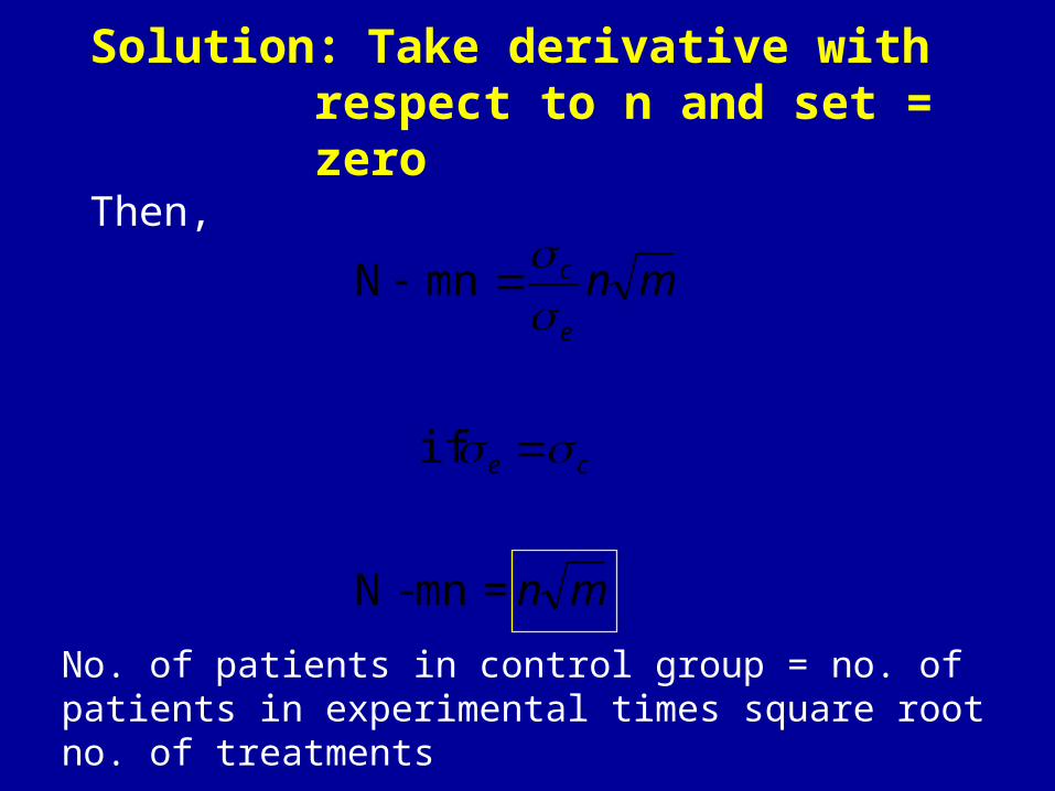
Solution: Take derivative with respect to n and set = zero

Then,

No. of patients in control group = no. of patients in experimental times square root no. of treatments

mn

mn

ce

e

c

=mn-N

if

mnN

Other Issues with Multiple Groups

• Multiple comparisons (a adjustment)

• Interim analyses – possible early termination of some, but not all, treatment groups

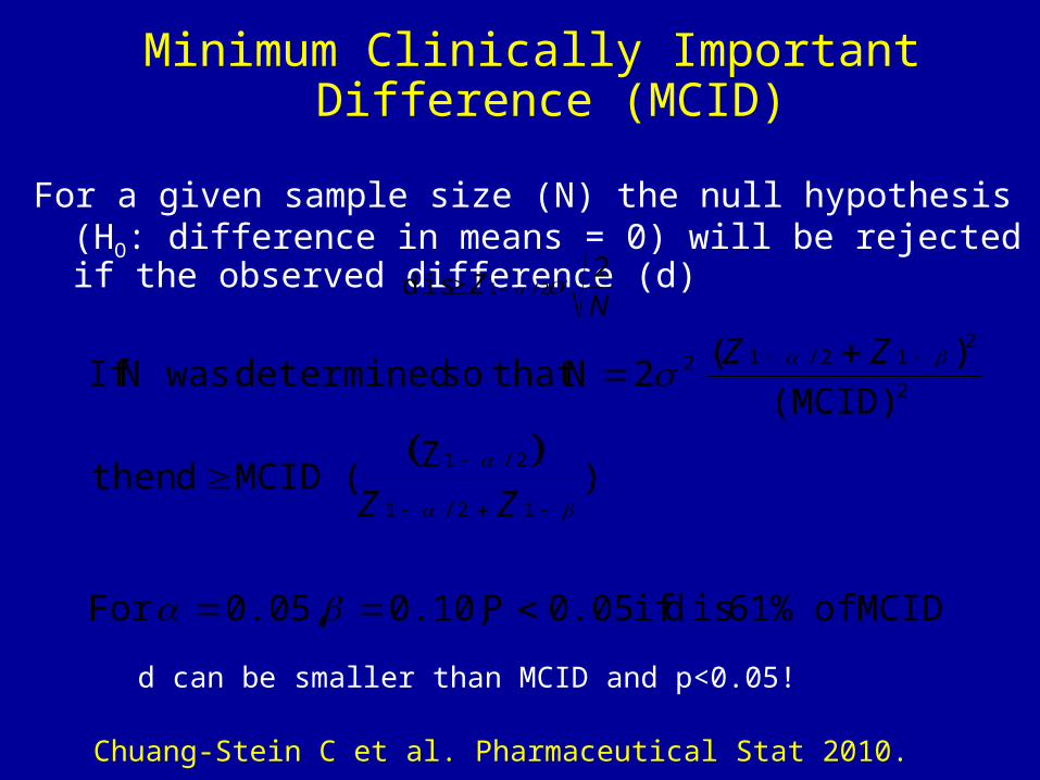
Minimum Clinically Important Difference (MCID)

For a given sample size (N) the null hypothesis (HO: difference in means = 0) will be rejected if the observed difference (d)

NZ

221 / is d

MCID of 61% is d if 0.05P 0.10, 0.05, For

)Z

( MCIDd then

(MCID))(

2N that so determined wasN If

12/1

2/1

2

212/12

ZZ

ZZ

Chuang-Stein C et al. Pharmaceutical Stat 2010.

d can be smaller than MCID and p<0.05!

Sample Size for Dual Criteria: Statistical Significance and Clinical Significance

• In some cases, you may want to establish with high probability that the treatment effect is as large as MCID

– For example, a new HIV vaccine might be assumed to have 60% efficacy but the study is designed to have sufficient power to rule out efficacy lower than 30%

– This will require a larger sample size

– For example, if Δ=2MCID, then sample size is 4 times greater

Summary (General)

• It is important that sample size be large enough to achieve the goals of the study – too many studies are conducted which are under-powered.

• Sample size assumptions are frequently very rough so they should be re-evaluated as the study progresses.

• A good knowledge of the subject matter (background on disease and intervention, outcomes, and target population) is necessary to estimate sample size.

Summary (Crossover versus Parallel Group)

• Efficiency of crossover increases as increases.

• Design using change from baseline as response is better than design which just uses follow-up responses if > 0.50.

• With multiple measurements on each patient, to establish baseline and follow-up levels, sample size can be reduced.