How Noise Trading Affects Markets: An Experimental Analysis

By

Robert Bloomfield, Maureen O’Hara, and Gideon Saar*

First Draft: January 2005 This Version: May 2007

*Robert Bloomfield (rjb9@cornell.edu), Maureen O’Hara (mo19@cornell.edu) and Gideon Saar (gs25@cornell.edu) are from the Johnson Graduate School of Management, Cornell University. Financial support for this project was obtained from New York University's Salomon Center for the Study of Financial Institutions. We would like to thank an anonymous referee, Matt Spiegel (the editor), Lucy Ackert, Joel Hasbrouck, Shimon Kogan, Wei Xiong, Halla Yang, and seminar participants at the NBER, New York University, Texas A&M, and the American Finance Association Meetings (Boston) for helpful comments.

Abstract

We use a laboratory market to investigate the behavior of noise traders and their impact on the market. Our experiment features informed traders (who possess fundamental information), liquidity traders (who have to trade for exogenous reasons), and noise traders (who do not possess fundamental information and have no exogenous reasons to trade). We find differences in behavior between liquidity traders and noise traders, justifying their separate treatment. We find that noise traders exert some positive effects on market liquidity: volume and depths are higher and spreads are lower. We provide evidence suggesting that the main effect of the liquidity-enhancing trading strategies of the noise traders is to weaken price reversals (decreasing the temporary price impact of market orders) rather than to reduce the permanent price impact of trades (as liquidity traders supposedly do in market microstructure models with information asymmetry). We find that noise traders adversely affect the informational efficiency of the market, but only when the extent of adverse selection is large (i.e., when informed traders have very valuable private information). Finally, we examine how trader behavior and certain market quality measures are affected by a transaction tax. Although such taxes do reduce noise trader activity, they take a toll on informed trading as well. As a result, while taxes reduce volume, they do not affect spreads and price impact measures, and have at most a weak effect on the informational efficiency of prices.

How Noise Trading Affects Markets: An Experimental Analysis

I. Introduction

Noise traders play a ubiquitous role in the finance literature. Fischer Black [1986]

dedicated his AFA presidential address to the beneficial effects of “noise” on markets,

concluding that “noise trading is essential to the existence of liquid markets.” Shleifer

and Summers [1990] and Shleifer and Vishny [1997] identified noise traders as the basis

for the limits of arbitrage, arguing that noise trading introduces risks that inhibit

arbitrageurs and prevent prices from converging to fundamental asset values. Noise

traders in the guise of SOES bandits have been credited with enhancing price discovery

(see Battalio, Hatch, and Jennings [1997] and Harris and Schultz [1998]), while their day

trading counterparts have been disparaged for creating speculative pressures in asset

prices both at home and abroad (Scheinkman and Xiong [2003]).1 Despite this attention

given to noise trading, there remains considerable debate regarding its precise role in

financial markets, and over whether society is well advised to limit noise trading by

taxation or other means, or to ignore it altogether due to its inconsequential nature in

affecting market outcomes.

Partially explaining this confusion is that two strands of the literature emerged in

the 1980s giving very different interpretations to the term “noise traders.” In the market

microstructure literature, researchers use the terms “noise traders” and “liquidity traders”

interchangeably to describe traders who do not possess fundamental information (e.g.,

Glosten and Milgrom [1985]; Kyle [1985]). While the motives of these traders are often

left unspecified, the justification for their trading is generally assumed to be some

1 See, for example, “Day Trading Makes a Comeback” (Reuters, December 19, 2004), where day traders “were blamed for adding irrationality to an exuberant market”. Similarly, critics of globalization point to excessive short-term speculation in foreign currency trading as undermining the economic viability of developing countries, a motivation also cited for Thailand’s recent (short-lived) imposition of a Tobin Tax on foreign exchange (see “Central Bank measure reminiscent of Tobin Tax”, The Nation, December 21, 2006).

2

hedging or liquidity needs that induce changes in traders’ optimal portfolio holdings.2

Alternatively, the limits-to-arbitrage literature champions the existence of traders in the

market who trade for reasons other than fundamental information, hedging, and liquidity

shocks. As Shleifer and Summers [1990] note, this literature adopted the term “noise

traders” to capture behavioral causes for trading not captured by these standard

explanations, and in fact labeled itself the “noise trader approach to finance.”

It is reasonable to conjecture that traders motivated by hedging or liquidity shocks

might behave differently from those who trade due to psychological biases or those who

simply have a taste for trading. Fisher Black in his presidential address was careful to

distinguish between these two types of traders, arguing that “People who trade on noise

are willing to trade even though from an objective point of view they would be better off

not trading. Perhaps they think the noise they are trading on is information. Or perhaps

they just like to trade.”

In this paper we seek to clarify the role and market impact of noise traders. To do

so, we construct a setting with three types of traders: informed traders (who possess

fundamental information), liquidity traders (who have to trade for exogenous reasons),

and noise traders (who do not possess fundamental information and have no exogenous

reasons to trade).3 We examine the impact of noise traders by comparing the behavior of

markets with noise traders to the behavior of markets without them. We also wish to

examine how efforts to curb such trading via taxation affect market and trader behavior.

2 Glosten and Milgrom [1985; pg. 77], for example, note that such trading “may arise from predictable life cycle needs or from less predictable events such as job promotions or unemployment, deaths or disabilities, or myriad other causes.” 3 The limits-to-arbitrage literature features noise traders who trade on the basis of mistaken fundamental information as well as noise traders who trade based on rules in the spirit of technical analysis (e.g., looking at past prices of the security). We chose to focus the experiment on the latter type of noise traders. The advantage of using experimental markets to investigate this issue is that we do not need to determine for the noise traders what strategies to adopt. For example, Shleifer and Summers [1990] motivate positive-feedback trading by citing research that shows how investors tend to extrapolate trends. However, studies that look at the trading of individual investors actually find contrarian tendencies (see, for example, Kaniel, Saar, and Titman [2006] and reference therein). The experimental approach provides traders with an economic environment but gives them complete freedom to adopt whatever technical strategies they believe will earn them more money.

3

The notion that short term speculation, presumably the hallmark of noise traders, drives

prices away from fundamental values has long been debated. Many countries impose a

transaction tax (“Tobin tax”) in order to curb such speculation, with the most recent being

Thailand’s ill-fated attempt to do so in December 2006. Stiglitz [1989] conjectured that

such a tax would work because it would be unlikely to discourage trading by those whose

trades are motivated by private information or liquidity needs, and so would mainly serve

to drive out the noise traders. Our experimental markets enable us to test Stiglitz’s

conjecture, as well as to investigate the effects of the tax on market liquidity and

informational efficiency.4

Experimental analysis seems particularly well suited for addressing the issues we

consider. Despite the extensive theoretical literature on noise trading, the complexity of

evaluating numerous (potentially non-rational) trading strategies imposes limitations on

even the most ambitious analyses (see, for example, the papers of DeLong, Shleifer,

Summers, and Waldmann (DSSW) [1990, 1990b, 1991] or the more recent work of

Scheinkman and Xiong [2003] and Lowenstein and Willard [2006]). Similarly, there is a

large empirical literature investigating the effects of particular trader types on markets

(see, for example, Garvey and Murphy [2001], Linnainmaa [2003], Barber et. al. [2004],

and Kaniel, Saar, and Titman [2006]), but the inherent problems with analyzing actual

market data (when such data is even available) makes inference problematic.

Experimental markets hold out the dual benefits of flexibility and control: traders are free

to choose whatever strategies they like, while confounding factors are held constant

across different market settings. This allows us to differentiate behaviors that are

otherwise difficult to disentangle, thereby yielding insights into the impact of noise

trading on financial markets.

4 For related papers on securities transaction taxes see Stiglitz [1989], Summers and Summers [1989], Amihud and Mendelson [1993], Schwert and Seguin [1993], Umlauf [1993], Subrahmanyam [1998], Dow and Rahi [2000], Habermeir and Kirilenko [2003], and Hinman [2003].

4

Overall, our evidence strongly suggests that noise traders behave very differently

from liquidity traders. We find that liquidity traders, who need to trade for exogenous

reasons, start a trading period more likely to use limit orders to trade, and as time goes

by turn to more extensive usage of market orders (i.e., switching from supplying to

demanding liquidity). Noise traders seem to behave in a different manner: their tendency

to trade by supplying liquidity actually increases throughout the trading period.

These differences in trading strategies also mean that the impact of noise traders

on market liquidity differs from that conjectured by many market microstructure models.

Decomposing the total price impact of market orders, we find that while decreases in

both permanent and temporary components contribute to the lower total price impact of

trades when noise traders are present in the market, the difference in the temporary price

impact is four to five times larger than the difference in the permanent price impact. This

evidence suggests that the main effect of the liquidity-enhancing trading strategies of the

noise traders is to weaken price reversals (decreasing the temporary price impact of

market orders) rather than to reduce the permanent price impact of trades (as liquidity

traders supposedly do in market microstructure models such as Glosten and Milgrom

[1985] or Kyle [1985]).

Looking at the informational efficiency of prices, we find that the presence of

noise traders increases pricing errors but only when the extent of adverse selection is

large. While worsening quality of prices is consistent with the notion expressed by Black

[1986] that noise traders “actually put noise into the prices,” the more intriguing result of

our experiment is that this effect is not observed unless informed traders have very

valuable information. The key for explaining this result lies in understanding the way

noise traders behave in markets.

We use our experimental data to shed light on the validity of three different ways

in which noise traders might behave. First, noise traders might act as skillful technical

traders who exploit information in the order book to earn a profit, as SOES bandits are

5

presumed to do in the analysis of Harris and Schultz [1998], or similarly they could use

information about price movements as uninformed traders do in the model of Hong and

Stein [1999]. Second, noise traders might rationally provide liquidity to the market,

providing a service to liquidity traders by adding risk-bearing capacity (i.e., acting as

market makers as in Grossman and Miller [1988]). Finally, noise traders might behave as

irrational traders who act as if they have information when they do not, as in the classic

description by Black [1986]. They could follow various technical trading rules or

“popular models” as in Shiller [1984, 1990], employing positive-feedback trading

strategies (e.g., De Long et al. [1990b]) or possibly behave as contrarians.5

Noise traders in our experiment appear to act as irrational contrarian traders.

Consistent with such behavior, adding noise traders dramatically increases market trading

volume, particularly when the fundamental value of the security (known collectively by

the informed traders) is far from the prior expected value. Skillful technical traders

would be expected to earn higher profits when values are extreme by exploiting any

sluggishness in price movements; however, our noise traders lose the most money when

values are extreme, because they act as (unwise) contrarians and as a result slow down

the adjustment of prices (worsening informational efficiency exactly when it is needed

the most).

Finally, we examine the effect of the securities transaction (Tobin) tax, both as a

lens to examine noise trader behavior, and to examine the effects of the transaction tax in

its own right. Not surprisingly, we find that the transaction tax dramatically reduces

trading volume. However, the tax reduces activity by noise and informed traders roughly

equally (contrary to the conjecture of Stiglitz [1989]), and perhaps as a result it does not

5 There is an empirical evidence that individual investors in various countries trade in a contrarian fashion (e.g., Choe, Kho, and Stulz [1999], Grinblatt and Keloharju [2000, 2001], Jackson [2003], Richards [2005], Kaniel, Saar, Titman [2006]). For experimental evidence consistent with contrarian behavior see Bloomfield, Tayler, and Zhou (2997).

6

alter bid-ask spreads or other price impact measures of liquidity, and has only a weak

effect (if at all) on the informational efficiency of prices.

Taken together, our results suggest that the many literatures that consider the

behavior of noise traders need to distinguish clearly between liquidity traders who trade

to meet liquidity needs, and “pure” noise traders who trade without information on their

own volition. Moreover, our results suggest that pure noise traders are likely to behave

as irrational contrarians, rather than skillful technical traders or rational liquidity

providers. Such traders provide markets with costs (decreased efficiency) and benefits

(increased liquidity for other traders) at their own expense. However, even if policy

makers were to conclude that noise trade is undesirable, our results raise doubts that

transaction taxes will provide much benefit.

The rest of this paper is organized as follows. The next section provides a more

detailed literature review and elaborates on the hypotheses we examine. Section 3 sets out

the experimental design. In Section 4 we present our results concerning the impact of

noise traders on market liquidity and the informational efficiency of prices. To help

explain the market-wide results, we also look at the trading strategies noise traders

pursue. Section 5 summarizes our results and offers conclusions on the role of noise

traders in financial market.

2. How Should Noise Traders Matter? Review and Hypotheses

Dow and Gorton [2006] suggest that the concept of “noise” traces back to the

Rational Expectations literature, where adding a random component to aggregate asset

supply made prices partially revealing. In such a non-revealing rational expectations

equilibrium, informed traders could profit from their trades, thereby providing at least a

partial answer to the Grossman-Stiglitz conundrum of how information-gathering is

compensated in an informationally efficient market. The notion of noise in that literature

is rather elusive in that it is not clear what economic phenomenon (e.g. a certain type of

7

agent or a certain type of shock that agents experience) is the source of this noise. What

matters in these models is simply that a mean-zero normally distributed random variable,

termed noise, influences aggregate supply.

The microstructure literature relies on a similar device to explain how prices do

not become instantaneously revealing. In the microstructure literature, “noise” is now

ascribed to specific trading behavior by uninformed traders. The Kyle [1985] model is

perhaps closer to the REE models, where the uninformed trades are viewed as a mean-

zero normally distributed random variable. The sequential trade models depart from this

normality framework, but employ the same concept of noise trade as exogenously given.

Both microstructure approaches require that uninformed traders must trade. Easley and

O’Hara [1987], for example, note that “If trades were solely information-related, any

uninformed trader would do better to leave the market rather than face a certain loss

trading with an informed trader. To avoid this no-trade equilibrium, we assume that the

uninformed trade (at least partially) for liquidity reasons. This exogenous demand arises

either from an imbalance in the timing of consumption and income or from portfolio

considerations”. This approach motivates our specification of the liquidity traders in the

experiment, who need to trade for an exogenous reason (that in an actual market would

corresponds to portfolio rebalancing, consumption, etc.).

In contrast, models following the “noise trader approach to finance” presume that

noise trade reflects irrational decision-making. Shiller [1984; 1990], for example, argues

that noise traders rely on “popular models” that are wrong and subject to fads. Shleifer

and Summers [1990] develop this further, arguing “Some investors are not fully rational,

and their demand for assets is affected by beliefs or sentiments that are not fully justified

by fundamental news.” DeLong, Shleifer, Summers and Waldman [1990] model noise

traders as those who misperceive the future value of the security. What can lead to such

misperceptions are a wide range of behavioral phenomena, such as overconfidence,

anchoring, representativeness, conservatism, belief perseverance, and the availability bias

8

(see Barberis and Thaler [2003]). Because of these behavioral factors, noise trading in

this literature can exhibit specific strategies that depend on past returns such as positive-

feedback trading (see, for example, Shiller [1994]; DeLong, Shleifer, Summers and

Waldman [1990b]).6 This literature motivates our specification of noise traders in the

experiment, who do not have private information about fundamentals and are not given

any trading targets. They are free to pursue whatever trading strategies they find

appealing in order to make money.

Our experimental design specifically aims to examine the behavior and market

impact of the noise traders while distinguishing them from traders driven by exogenous

liquidity shocks, whom we call “liquidity traders.” We do so by creating a laboratory

market that includes informed traders who are given private information about each

security’s liquidating dividend, liquidity traders who must achieve a predetermined

trading position in each market period, and noise traders who have neither information

nor trading targets (and can therefore pursue any trading strategy they choose, but lack

any objective informational advantage).7

We have three goals in this study. Our first is to examine the impact of noise

traders on market liquidity and the informational efficiency of prices. Because we are not

ascribing any particular behavioral bias to noise traders, our second goal is to characterize

how noise traders behave. Our third goal is to examine how securities transaction (Tobin)

taxes affect the behavior of traders and overall market activity. Imposing transaction

taxes helps us further understand the behavior of noise traders (because different sources

of noise trade suggest different effects) and can also aid in investigating the potential 6 The literature on heterogeneous agents also focuses on noise traders as trend chasers. These models (see for example Brock and Hommes [1998]; Lux [1995]; Lux and Marchesi [2000]) investigate bubbles and crashes, and feature fundamental traders versus noise traders. In these models, it is the noise traders who induce the aberrant market behavior. 7 Note that by having liquidity traders in the experiment, we probably underestimate somewhat the potential (or need) for liquidity provision by the noise traders. However, like the majority of papers in finance, be believe that traders who trade for portfolio rebalancing and consumption (our liquidity traders) are indeed present in the market. Hence, our goal is to examine the trading activity of the noise traders and their impact on market outcomes in a market that is already populated by liquidity and informed traders.

9

impact of such taxes on financial markets. In the following sub-sections, we develop

some specific hypotheses regarding noise trading and its effect on liquidity and

informational efficiency. We also attempt to sort out the various motivations for noise

trading by considering some hypotheses for the noise traders’ trading strategies.

2.1. Liquidity

A market’s liquidity is generally captured by a vector of attributes such as

volume, depth, spreads, and the price impact of market orders. In sequential trade models,

greater activity by liquidity traders reduces the bid-ask spread (which is equivalent to the

permanent price impact of trades in these models) by decreasing the expected information

content of each trade (because more trades can be driven by a liquidity shock as opposed

to information). However, if informed traders concomitantly increase their trading (as

predicted by Kyle [1985]) then spreads (or the permanent price impact) may be

unaffected by changes to liquidity trading. Liquidity traders may also reduce depth if they

use market orders to ensure that they are able to hit their trading targets, and cancel their

limit orders to avoid having excess executions in the closing moments of trade (as

observed in Bloomfield, O’Hara and Saar [2005]).

The impact of noise traders on market liquidity is not obvious. Conceptually, their

impact could be similar to that of the exogenously-specified liquidity traders in Glosten

and Milgrom [1985], who reduce the permanent price impact of trades. Alternatively, in

Grossman and Miller [1988] and Campbell, Grossman, and Wang [1993], the presence of

uninformed risk-averse traders reduces the temporary price impact of trades.

Distinguishing between the permanent and temporary price impacts could speak to the

differences in behavior between (target-induced) liquidity traders and (potentially risk-

averse) noise traders. In our analysis we decompose the total price impact of trades to

sort out these two competing hypotheses of trader behavior.

The effect of noise traders on liquidity may also depend on the nature of their

trading activity. Noise traders who act as rational liquidity providers may increase trade

10

volume as they simply supplant other traders as a source of liquidity (similar to the

“multiplier effect” that dealers have on reported market volume). They will also increase

order book depth and reduce the temporary impact of trades. Such a prediction is

reasonable, as Linnainmaa [2003] concludes that day traders extensively supply limit

orders, suggesting that liquidity provision is a potential source of profit for noise traders.

Noise traders who act as skillful technical traders are likely to use market orders to

exploit their short-lived informational advantage; this will increase volume, but also

increase bid-ask spreads (because they are taking limit orders, rather than providing

them). Finally, noise traders who trade as contrarians for behavioral reasons will increase

volume, and will also reduce the temporary price impact as they attempt to reverse recent

price movements. Noise traders who act as momentum traders will increase bid-ask

spread and temporary price impacts as they pile on to prior trades.

2.2. Informational Efficiency

All three theoretical approaches to noise trading (i.e. rational expectations models,

market microstructure models, and limits-to-arbitrage models) have similar predictions

with respect to informational efficiency. Greater exogenous liquidity trading it is

expected to reduce the informational efficiency of markets and slow down the adjustment

of markets to private information. This detrimental effect arises because liquidity trading

reduces the probability that a given trade is motivated by information. Noise traders who

rationally provide liquidity to the market, or who trade for behavioral reasons, would

presumably have similar effects.

However, noise traders who extract information from the order book (that for

some reason other traders miss) can ‘pile on’ to price trends, helping prices adjust faster

to information. This effect was especially stressed in the controversy over SOES bandits

who picked off dealers whose quotes were slow to adjust to market conditions (see

Battalio, Hatch, and Jennings [1997] and Harris and Schultz [1998]). Black [1986] also

mentions this view, noting that “The move [of prices back towards their (true) value] will

11

often be so gradual that it is imperceptible. If it is fast, technical traders will perceive it

and speed it up.” Hence, noise traders acting as skillful technical traders would likely

help prices move towards true values.

2.3. Profits

A central question in the literature on day traders, who are presumably the most

similar to the pure noise traders we examine in our experiment, is whether their activity is

profitable. Empirical evidence provides a mixed picture. Harris and Schulz [1998] and

Linnainmaa [2003] show that day traders make profits, while Jordan and Diltz [2003]

and Barber et al [2004] document that they lose money on average. These competing

findings reflect the ambiguity of our profit predictions, which depend on the motivation

for noise trade.

Skillful technical traders and rational liquidity providers would be expected to

earn positive trading profits overall (otherwise they would not rationally trade).

However, the pattern of their profits will vary. Technical traders who ride price

momentum will make their greatest profits when the appropriate price adjustment is very

large (and technical traders anticipate that movement). These gains might be offset partly

by losses when appropriate price movements are small. In contrast, liquidity providers

will earn their greatest profits when appropriate price movements are small, so that they

can earn money by providing liquidity without losing to better-informed traders. Those

gains will be partly offset by the losses they incur when appropriate price movements are

large, and they face larger adverse selection from informed traders. Behavioral noise

traders would be expected to lose money overall. Whether their losses are greatest when

fundamental values are extreme or moderate depends on whether they are momentum or

contrarian traders.

2.4. Securities Transaction Taxes

We also examine how the imposition of a securities transaction (Tobin) tax would

affect market behavior and trader profits. Proponents of the tax often claim that trades of

12

short-term speculators are destabilizing because they move prices farther away from true

values, and that the tax would improve the efficiency of prices without harming liquidity.

Arguments on the potential costs and benefits of a securities transaction tax can be found

in Schwert and Seguin [1993], Pollin, Baker, and Schaberg [2002], and Haberman and

Kirilenko [2003]. In our experimental markets it is straightforward to test for the impact

of transaction taxes on informational efficiency and liquidity because we know the

securities’ “true value” and whether specific trades move prices toward or farther away

from this value.

Stiglitz [1989] conjectures that the tax is unlikely to discourage trading by those

motivated by private information or liquidity needs, and so would mainly serve to drive

out the noise traders. Constantinides [1986] argues that the imposition of a tax should

lower trading volume, and Umlauf [1993] provides empirical evidence to support this

effect. How this lower volume will affect market liquidity is less clear. If Stiglitz’s

conjecture is correct, then spreads might be expected to increase to reflect the higher

relative importance of informed trade in the overall order flow. However, Subrahmanyam

[1998] and Dow and Rahi [2000] argue that informed traders will trade less under the tax

regime, and so spreads could be unaffected or even fall.

The design of our experiment ensures that the tax we impose would have no effect

on the liquidity traders, because the transaction tax is presumably small relative to the

incentives to achieve the target trading position. As for the noise traders, taxes should

suppress rational noise trade far more than they would suppress informed trade, because

both skilled technical trading and liquidity provision have smaller potential profits than

trading on private information about fundamentals. In particular, a liquidity-providing

noise trader needs to both buy and sell to make a profit (paying taxes on both

transactions), while an informed trader in our markets can actually hold the security until

receiving a liquidating dividend (and hence avoid paying the tax for closing the position).

The effect of the tax is far less clear for behavioral noise traders; however, to the extent

13

that they believe they have valuable information, their reactions to the tax will be similar

to those of (truly) informed traders.

3. Experimental Design

We now describe the nature of our experiment and the specific features of our

markets. As a useful preliminary, we note the following definitions. A cohort is a group

of traders who always trade together. A security is a claim on a terminal dividend, and is

identified by the liquidating dividend, distribution of information and liquidity targets

(described below). A trading period is an interval during which traders can take trading

actions for a specific security. Only one security is traded in each trading period. Unless

otherwise indicated, all prices, values, and winnings are denominated in laboratory

dollars ($), an artificial currency that is converted into US currency at the end of the

experiment.

3.1. Experimental Goals, Task and Design

We seek to understand the behavior, welfare, and market influence of noise

traders. To do so, we create markets for the trading of securities. Each security pays a

liquidating dividend equal to 50 plus the sum of five random numbers, each of which is

uniformly distributed from -15 to 15. Values are truncated to lie in the range [0, 100],

resulting in the roughly bell-shaped distribution shown in the instructions to participants

in Appendix A. Trading in each security lasts for 120 seconds.

Trader types are defined as follows. There are four informed traders in the

market. Two informed traders observe the sum of the true liquidating dividend plus a

predetermined random number (different for every security) drawn from the interval [-10,

10], while the other two observe the sum of the true liquidating dividend minus the same

predetermined random number for that security.8 This structure guarantees that each

8 We perfectly balanced the size of the predetermined random number (large versus small) across the within-subject factors in the experiment.

14

informed trader has imperfect information about security value, but that the informed

traders in the aggregate have perfect information. Imperfect information means that

trading on private information is still risky for the informed traders (before prices fully

adjust), while aggregate certainty simplifies the trading task (Lundholm [1991]), and

guarantees that the rational expectations equilibrium price is equal to the true liquidating

dividend.

There are four liquidity traders in the market. Liquidity traders are only told the

prior distribution of dividends. They are assigned trading targets (in terms of number of

shares) they must achieve before the end of trading if they are to avoid a penalty equal to

$100 for each unfulfilled share. To limit their ability to speculate, liquidity traders are

prohibited from buying shares if their target requires selling, and are prohibited from

selling shares if their starting target requires buying.9 The liquidity targets are random,

with two-thirds of the securities resulting in a non-zero net liquidity demand.10

Noise traders have the same informational disadvantage of liquidity traders, but

face no trading targets. These noise traders fit the definition offered by Black of traders

who may “simply like to trade”, but such noise trading may also be motivated by traders’

beliefs that they can interpret market information better than others, or that they can earn

profits by providing liquidity (due to the non-zero aggregate net demand by liquidity

traders in two-thirds of the securities).11

9 The use of trading targets is standard in experimental work (see Lamoreaux and Schnitzlein [1997], Cason [2000], Bloomfield and O’Hara [1998; 2000] and Bloomfield, O’Hara and Saar [2005]), and it captures the notion that liquidity traders are transacting for exogenous reasons relating to the need to invest or the need to liquidate positions. 10 For 8 securities, half of the liquidity traders must buy 20 shares and the other half must sell 30 shares, for an aggregate liquidity demand of −20. For another 8 securities, half of the liquidity traders must sell 20 shares, while the other half must buy 30 shares, for an aggregate liquidity demand of +20. The remaining eight securities have zero aggregate liquidity trader demand: for 4 of those securities, half of the traders must buy 20 shares and the other half must sell 20 shares; for the other 4 securities, half of the traders must buy 30 shares, and the other half must sell 30 shares. 11 Each trader knows his or her type, and each knows the populations of informed, liquidity, and noise traders in the market. Traders do not know the roles played by specific participants in the experiment.

15

Our experimental design manipulates factors both between cohorts, and between

securities within each cohort. As shown in Panel A of Table 1, our between-cohort

manipulations include trader composition and tax treatment order. Six cohorts are

composed of four informed traders and four liquidity traders, while the other six cohorts

are composed of four informed traders, four liquidity traders, and four noise traders. Half

of the cohorts of each composition trade in the presence of transaction taxes during the

first block of securities (block 1) and then in their absence (block 2), while the other half

trade in the absence of transaction taxes during block 1 and in their presence in block 2.

Panel B of Table 1 describes the factors that we manipulate between securities

within each cohort. These factors are the transaction tax regime and the extremity of the

realized value of the security. In the transaction tax regime, we impose a $2 tax on each

side of every transaction. No taxes are assessed on trading when the transaction tax

regime is not in effect.12 We assess whether the security value is “high” or “low”

extremity by calculating the absolute deviation of the liquidating dividend from 50,

which is the prior expected value of the security. The extremity factor (how different the

realized value of the security is from its unconditional mean) has two levels: High

Extremity (realized values that are at least $17 from expected value) and Low Extremity

(realized values that are no more than $16 from expected value).]; the twelve securities

with a more extreme value are coded as high extremity, while the remaining twelve are

coded as low extremity. Extremity of the realized value of the security is used as a

measure of the value of the informed traders’ private information; the farther away the

security value is from its expected value, the more the informed traders can profit from

their information.

12 As discussed above, half of the cohorts trade with taxes in block 1 and without taxes in block 2, while the other cohorts trade without taxes in block 1 and with taxes in block 2. This means that whether the tax regime is introduced early or late in the session is completely balanced across cohorts, and we also statistically test for any order effects.

16

As indicated in Panel B of Table 1, we fully cross the tax and value extremity

factors to allow for six securities in each cell of an orthogonal 2 (tax regime) x 2 (value

extremity) design within each cohort. All cohorts trade the securities in the same order.

Securities in the same transaction tax block are contiguous, but securities are otherwise

ordered unpredictably, so that participants cannot anticipate the value extremity of

upcoming securities. Securities also vary according to their realization of aggregate net

demand of the liquidity traders, which can be +20, –20 or 0. We balance aggregate net

demand with our other factors by ensuring that there is no significant correlation of

aggregate net demand with the other factors.13

3.2. Trading

Each security is continuously traded in a trading period that lasts two minutes.

Our double auction market is organized like a typical electronic limit order book where

traders can enter buy or sell limit orders and the execution of limit orders follows strict

price/time priority rules. This means that a limit order at a better price (for example, a

higher price for a buy order) has priority over a limit order at a worse price. Within each

price level, older limit orders are executed first. Traders can execute outstanding limit

orders in the book by clicking a “buy 1” button, which allows them to buy one share at

the lowest current asking price, or by clicking a “sell 1” button, which allows them to sell

one share at the highest current bid price. Executing a limit order in the book is

equivalent to submitting a market (or marketable limit) order.

Limit orders to buy or sell a security must have integer prices between 0 and 100.

As soon as a trader enters an order, the order is shown on all traders’ computer screens,

indicating that an unidentified trader is willing to buy or sell one more share at the posted

price. Traders can cancel their unexecuted limit orders in the book at any time during the

13 A prior experiment indicates that realizations of aggregate net demand do not qualify the effects of taxes and value extremity on the behavior and impact of noise traders in a setting very similar to that examined here. Therefore, we expect this imperfect balancing technique to be adequate and allow clean inferences.

17

trading period. All trades are reported immediately to all traders, indicating the price and

the trade direction (whether the trade involved a market buy taking a limit sell order or a

market sell taking a limit buy order). The colorful, mouse-driven, graphical interface

(nearly identical to that used in Bloomfield, O’Hara and Saar [2005], and shown in

Figure 1), allows for very rapid trading, as traders need not type in orders or

cancellations, and can see at a glance whether market activity or the order book has

changed.14 Traders can also continuously observe on the screen their current position (in

terms of shares and cash), the number of shares they bought or sold, and the average price

they paid for the shares they bought or sold.

3.3. Subjects, Training, and Incentives

The experiments were conducted in the Business Simulation Laboratory (BSL) at

the Johnson Graduate School of Management at Cornell University, using a mixture of

MBA and undergraduate students.

All participants experienced intensive training for the experiment. Participants

first attended a 90-minute training session, which began with 5-10 minutes in which

traders could read the written instructions provided in Appendix A and 15-25 minutes of

oral review of those instructions. The remaining time was devoted to allow participants

to trade securities in each of the three roles (informed trader, liquidity trader, and noise

trader) in markets of up to 20 traders. A total of 120 participants returned for a second

session, which began with about 15 minutes of review (silent reading of instructions,

review of key points, and one practice security). The remaining time was devoted to

trading the 24 securities from which our data are drawn.

14 A trader’s screen includes one chart indicating bids (limit buy orders) and one indicating asks (limit sell orders). The left side of each chart shows every price at which an order has been posted (shown in green for the highest bid and lowest ask price, and yellow for other prices), and the number of shares posted at that price (shown by a number to the left of the graph). The right side of each chart shows every price at which the trader has personally posted an order, and the number of shares that the trader has posted at that price. The center of each chart also includes a solid red line indicating the highest bid or lowest ask entered by any trader, and a solid green line indicating the highest bid or lowest ask entered by that particular trader.

18

Traders started trading in each security with zero endowments of cash and shares.

Unlimited negative cash and share balances were permitted, so traders could hold any

inventory of shares they desired, including short positions. The unlimited ability to short-

sell balances the unlimited ability to borrow, eliminating the risk of price bubbles driven

by excess cash in the market (as observed by Caginalp et al [2001]). Traders were told

that at the end of trading shares paid a liquidating dividend equal to their true value. A

trader’s net trading gain or loss for a security would then equal the value of their final

share holdings plus or minus their ending cash balance. Any penalties assessed to a

liquidity trader for failing to hit a target are deducted from this trading gain or added to

her trading loss. When applicable, transaction taxes are also subtracted from the trading

profits or losses of traders.

Each participant was paid $60 plus or minus one dollar for every 1000 laboratory

dollars gained or lost through trading, taxes and penalties, to a minimum of $5. This

minimum was paid to only four of the 120 subjects, indicating that most traders likely did

not engage in risk-seeking behavior due to the truncation of downside risk. Participants

were told the explicit formula used to compute their winnings (see instructions in

Appendix A), to ensure that participants unambiguously understood the incentives in the

experiment (and how they relate to trading).

4. Noise Trading in Financial Markets: Results

Our experimental framework is designed to investigate how noise traders affect

market behavior, how they behave, and how their influence and behavior is affected by

transaction taxes. We use this data, along with analysis of their trading profits, to draw

inferences about how noise traders differ from liquidity traders, and whether they tend to

be skillful technical traders, liquidity providers, or behavioral momentum or contrarian

traders.

19

In general, we find that all three trader types (informed, liquidity, and noise) trade

using a mix of market and limit orders. This evidence suggests that experimental subjects

understood the market mechanism and felt comfortable pursuing various order strategies.

We also observe that our markets are “well-behaved” in that pricing errors tend to decline

over the trading period, order flows and volume exhibit the usual patterns observed in

prior studies, and spreads generally decrease over time. Investigating our hypotheses

requires a thorough statistical analysis, and as a useful preliminary, we first discuss the

statistical methodology we employ before turning to our results.15

4.1 Statistical Analysis

Our analysis relies on repeated-measures ANOVA. From a statistical standpoint,

the repeated-measures ANOVA is a conservative and robust procedure for analyzing

experimental data. For analyses of market-level variables, such as market prices and

market liquidity, we judge statistical significance by computing the average of the

dependent variable within each cell (defined by the appropriate factors) for each of the

cohorts. A repeated-measures analysis effectively treats each cohort as providing a single

independent observation of the dependent variable. This design reduces the problem,

common in experimental economics, of overstating statistical significance by assuming

that repetitions of the same actions by the same group of subjects are independent events.

Therefore, our statistical analysis for market-level variables has a factorial structure 2

(noise) x 2 (extremity) x 2 (tax), for the existence of noise traders in the market,

extremity of the realized value of the security (high versus low), and imposition of the

transaction tax (with versus without tax), respectively.

For analyses of individual-level variables (such as order-submission rates), we

judge statistical significance by computing the average of the dependent variable within 15 Appendix B contains figures with (i) use of limit and market orders for each trader type, (ii) behavior of volume and pricing errors over the 24 securities in a session, and (iii) transaction prices for all securities traded by all cohorts. These are presented for the sake of completeness. Section 4 and all numbered tables and figures in the paper present results and statistical analysis that focuses on our particular hypotheses about noise trader behavior and their impact on the market.

20

each cell (defined by the appropriate factors) for each of the participants. Our statistical

analysis for individual-level variables has a factorial structure of 2 (type) x 2 (extremity)

x 2 (tax) for the cohorts with just two types of traders (informed and liquidity), or 3 (type)

x 2 (extremity) x 2 (tax) for cohorts with three types of traders (informed, liquidity, and

noise). In a few cases we also computed the variables of interest separately for ten 12-

second time intervals within the trading period. For these variables we add another factor,

time, to the ANOVA (e.g., for analysis of market-level variables the structure becomes

2 (noise) x 2 (extremity) x 2 (tax) x 10 (time)).

We repeated all the analyses testing for the influence of another factor: the order

of the tax blocks in the experiment (i.e., whether subjects first traded securities under the

tax regime and then without taxes, or vice versa). In almost all cases the effect of this

factor was not significant, and therefore we omit it from the presentation of the results.

Only in one variable did we find this factor to matter, and we note this finding in our

discussion of this particular variable in Section 4.3.

We present all statistically significant main effects and interactions from the

repeated-measures ANOVA analysis in the tables and figures. A main effect examines

the influence of one factor averaging over all the levels of the other factors. An

interaction is when the effect of one factor is different at different levels of the other

factors.16 In the text of the paper, we provide the p-value for the main effects in

parentheses without specifically mentioning the factor (it can be understood from the

context of the sentence), while interactions are specifically stated in parentheses next to

the p-values. Lastly, in a few of instances where the variables under investigation can be

either positive or negative (e.g., trading profit), we also provide in the tables indication of

statistical significance against the hypothesis of a zero value using a t-test.

16 For example, a significant extremity main effect without a significant type*extremity interaction means that extremity of the realized value (high versus low) exerts a similar influence on the behavior of all trader types. A significant type*extremity interaction implies that the different types of traders behave differently in high and low extremity securities with respect to the dependent variable under investigation.

21

4.2 Market Liquidity

Our first set of tests investigates how noise trading affects market liquidity, as

captured by volume, depth, and measures of transactions costs (spreads and the price

impact of market orders).

4.2.1 Volume

As expected, the amount of trading in the market is significantly influenced by the

inclusion or exclusion of noise traders, and by the presence or absence of a transaction

tax. Panel A of Table 2 shows that volume is greater in securities traded by noise traders

(p-value = 0.0053), and volume is lower in securities traded under the tax regime (p-value

= 0.0140). The results also show that there is a significant interaction between extremity

and noise trading (p-value = 0.0158). In particular, volume is higher for high extremity

securities only when there are noise traders in the market. This finding suggests that

noise traders are more active when security prices appear to be farther away from their

expected values, consistent with their acting as either rational momentum traders (who

are reacting quickly to price movements), or as behavioral traders who fail to protect

themselves from the adverse selection that arises when security values are extreme.

Panel B of Table 2 shows that adding noise traders to a market has little effect on

the trading of the liquidity traders (who are constrained to trade the same number of

shares in all cells of the design), but it does allow informed traders to increase their

trading activity. Perhaps more intriguing is what happens to trading activity when there is

a securities transaction tax. In the absence of noise traders, informed traders trade much

less when taxes are imposed, while liquidity traders, with their exogenous trading

requirements, are little affected (type*tax p-value = 0.017). When noise traders are

present in the market, these same effects arise, with noise trading decreasing by 23% but

informed trading falling by 28% (type*tax p-value = 0.0175). The significant interaction

is due to the fact that liquidity traders do not change their trading intensity. When we

eliminate the liquidity traders from our statistical analysis, we find that transaction taxes

22

affect the willingness to trade of informed and noise traders about equally (type*tax

interaction p-value = 0.3548). These results suggest that noise traders believe that they

have the ability to infer very useful information from market data—if they were

rationally engaging in short-term technical strategies or liquidity provision, they would be

deterred by Tobin taxes more than the informed traders are.

4.2.2 Depth

Another dimension of market liquidity is displayed liquidity in the limit order book.

Table 3 provides data on average depth at the best bid or offer (BBO) prices, which we

use as a measure of displayed liquidity.17 We find that noise trading dramatically

increases depth, both in the tax and no-tax settings (p-value = 0.0009). In the no-tax

setting, adding noise traders doubles the depth at the best bid or offer prices, suggesting

that noise traders are actively submitting limit orders that match or better the BBO. The

overall effect of noise traders on depth could suggest that they are rationally providing

liquidity to the market. Consistent with this view, we also observe that greater adverse

selection, which we measure by the value of the informed traders’ private information

(the extremity manipulation), reduces depth (p-value = 0.0019), which is in-line with the

hypothesized impact of information asymmetry in the market microstructure literature.

An interaction of noise, extremity, and taxes shows that while taxes tend to decrease

depth in the book, this need not always occur (noise*extremity*tax p-value = 0.0046).

4.2.3 Spreads and Price Impact

We look at two measures of transactions costs in our markets: spreads and price

impact of market orders. In general, spreads exhibit the usual shape in that they start high

and decline throughout the trading period until the very end, when they increase slightly. 17 Looking at BBO depth has a few advantages over analyzing total depth in the book. Total depth is influenced by stale limit orders: when market prices are running away from a trader’s limit orders, the trader would often submit more aggressive limit order but would not necessarily bother to cancel stale orders. Also, traders would submit limit orders away from current prices in an attempt to game other participants to believe that the true value resides elsewhere. We want a measure of displayed liquidity that represents actual commitments of traders, and BBO depth seems a particularly appropriate measure for this purpose (see also Bloomfield, O’Hara, and Saar [2005]).

23

This end-of-period effect is due to the increased use of market orders by liquidity traders

(who have to trade) coupled with the cancellation of limit orders by liquidity traders who

have reached their trading targets (see Bloomfield, O’Hara and Saar [2005] for a

discussion of these effects). To examine the behavior of spreads over the trading period,

we divide the trading period into ten time intervals and compute time-weighted spreads

separately for each interval. Figure 2 shows the behavior of spreads over time.

The data reveal a significant noise*extremity*time interaction (p-value = 0.0304),

so we analyze the behavior of spreads across four experimental regimes: no noise traders

/ low security value extremity (LNLE); no noise traders / high extremity (LNHE); noise

trade / low extremity (HNLE); noise trade / high extremity (HNHE). The data do not

indicate any tax interactions, so we do not segment the results according to tax regimes.

Market microstructure models suggest that spreads will be affected by the extent of

asymmetric information, which in our model is partially captured by the extremity

variable that represents the value of the private information. As expected, we observe an

extremity affect consistent with predictions of market microstructure models. Our main

interest is in how noise trading influences these spreads. The data clearly indicate that

when noise traders are present, spreads are lower. In Figure 2 the bottom two lines

correspond to spreads with noise trading, and these almost always lie below the spreads

in markets without noise traders. Closing spreads (not reported) are also lower when

noise traders are present.18 Notice that this result is similar in principle to the predicted

effect of (exogenous) liquidity traders in market microstructure models (e.g., Glosten and

Milgrom [1985] and Kyle [1985]), where liquidity traders are shown to affect the

permanent price impact of market orders (and hence the spread).

18 Closing spreads (the spread in the limit order book at the end of trading) also exhibit a significant noise*extremity interaction (p-value = 0.0426) and these closing spreads are lower when there are noise traders in the market.

24

To gain more insight into how noise traders are affecting the market, we decompose

the price impact of market orders into temporary and permanent price impacts (attributed

to liquidity provision and information, respectively). This type of decomposition is often

used in the empirical market microstructure literature. For a market order placed at time t

denote the transaction price by Pt, the midpoint between the best bid and offer prices in

the limit order book (just before the trade) by Mt, and the midpoint between the best bid

and offer prices prevailing five trades after the market order for which we are computing

the price impact by Mt+5. The total price impact for a buy (sell) order is defined by Pt –

Mt (Mt – Pt). The permanent price impact for a buy (sell) order is defined by Mt+5 – Mt

(Mt – Mt+5) and the temporary price impact is defined by Pt – Mt+5 (Mt+5 – Pt). Note that

the total price impact is the sum of the permanent and temporary components.

Figure 3 shows that the price impact measures are greatly affected by the presence

of noise trading, with the most visually striking effect being the significantly lower

temporary price impact when there are noise traders in the market (p-value = 0.0312).19

While decreases in both the permanent and temporary price components contribute to the

lower price impact of trades in securities when noise traders are present, the difference in

the temporary price impact is four to five times the magnitude of the difference in the

permanent price impact. For example, low extremity securities have a temporary price

impact of $2.93 and a permanent price impact of $0.45 without noise traders, and these

drop to $1.49 and $0.28, respectively, when noise traders are in the market. This

evidence suggests that noise traders do make the market more liquid, and in particular

their activity makes reversals due to illiquidity (the temporary price impact) smaller. In a

sense, their greatest impact is not the reduction of permanent price impact (as the

exogenous liquidity traders do in Glosten and Milgrom [1985] and Kyle [1985]), but

19 Since the permanent and temporary components can be negative as well as positive, we also tested to see if the values of these components are different from zero. The tests indicated that the temporary and permanent price impact components are significantly different from zero at the 1% level in all cells.

25

rather the risk-averse provision of liquidity as in the models of Grossman and Miller

[1985] and Campbell, Grossman, and Wang [1993].

Our results on spreads and price impacts show that noise traders do enhance market

liquidity, a finding consistent with noise traders acting as rational liquidity providers or

behavioral contrarian traders, but less consistent with them performing as skillful

technical traders or behavioral momentum traders. We do not find evidence that

informed traders completely offset the activities of noise traders as predicted by Kyle

[1985]. A securities transaction tax does limit the activity of noise traders, but also affects

the informed traders, consistent with the models of Subrahmanyam [1998] and Dow and

Rahi [2000]. We do not find a significant effect of taxes on spreads, although taxes do

dramatically reduce volume.

4.3 Noise Traders and Informational Efficiency

The informational efficiency of a market refers to how well, and how quickly,

market prices reflect true values. There are several ways to measure such efficiency, but

perhaps the most straightforward manner is to consider pricing errors, or the average gap

(in absolute value) between transactions prices and the true value, which we denote by

DEVP. Figure 4 shows the patterns in pricing errors over the trading period separately

for the four noise / extremity groups defined earlier.

Figure 4 demonstrates that pricing errors decline throughout the trading period

(from time interval 1 to 10) as prices incorporate more of the informed traders’

information. There is also a significant interaction of extremity*time (p-value < 0.0001):

pricing errors for high extremity securities start much higher and converge in a more

dramatic fashion. Pricing errors for low extremity securities naturally start smaller (as

26

prices at the beginning are closer to the prior expected value of 50), but they also

decrease with time on average.20

Our discussion in Section 2 suggested the hypothesis that noise traders reduced a

market’s informational efficiency. Table 4 provides evidence on this issue. For high

extremity securities, this hypothesis is clearly supported: the presence of noise traders

increases the pricing errors in both the tax and no-tax regimes. However, for low

extremity securities, this effect is not found. Adding noise trading to these markets does

not increase pricing errors, and may even decrease them slightly (noise*extremity p-value

= 0.0262).

Since noise traders add more liquidity to a market, it is possible that the small

decrease in pricing errors we observe in low extremity securities comes simply from

smaller spreads. To examine this possibility, we look at a different definition of pricing

error, DEVMID, computed as the distance of the true value from the prevailing mid-

quote when a transaction occurs. We find that DEVMID pricing errors for low extremity

securities are about the same with and without noise traders (4.5 and 4.4, respectively).

This is consistent with our conjecture that the lower DEVP pricing errors for low

extremity securities are due to better liquidity (and lower spreads). However, the

influence of noise traders on pricing errors computed from mid-quotes in high extremity

securities is similar to that found with DEVP: noise traders worsen informational

efficiency when there is more information in the market. We interpret this evidence as

suggesting that noise traders worsen the informational efficiency of the market exactly

when it is most important (i.e., when the value of new information is large).

It is interesting to note that there is no statistically significant effect of the tax on

the average pricing errors measure, although there is a small effect if we simply look at

20 While Figure 4 shows that the decline for low extremity securities is much smaller in magnitude that the decline for high extremity securities, analysis of ANOVA simple effects reveals a statistically significant decline for DEVP in each of our noise*extremity cells.

27

pricing errors computed from end-of-period prices. As we noted in Section 4.1, the order

of the tax treatment (i.e., whether subjects first traded securities under the tax regime and

then without taxes, or vice versa) did not matter for all our variables, except for marginal

effects if pricing errors are computed from end-of-period prices (CLSDEV).21

An alternative approach to evaluating informational efficiency is to consider how

the actions of individual traders contribute to value discovery, or the evolution of

transaction prices toward the true value of the security. To compute the measures

INFEFF, we assign +1 or –1 to each executed order in the following manner. If the true

value is higher than the price, we assign +1 to a buy order of a trader that resulted in a

trade and −1 to a sell order that resulted in a trade. If the true value is lower than the

price, we assign −1 (+1) to a buy (sell) order of a trader that resulted in a trade. The

measure is then aggregated for all market and executed limit orders of a trader and

divided by the number of his trades (the measure is therefore always in the range [−1,

+1]). The more positive (negative) INFEFF of a trader, the more his trades contribute to

(interfere with) value discovery.

Table 5 shows, not surprisingly, that informed traders help prices converge to true

values, while liquidity traders hinder this effect (as is predicted by market microstructure

models). Noise traders affect the market differently depending upon the degree of

adverse selection. When there is not much adverse selection (extremity value is low),

noise traders do not interfere much with value discovery (–0.04 for the noise traders,

which is not statistically different from zero, as opposed to –0.13 for the liquidity

traders). When the value of information is high, noise traders greatly hinder value

21 In sessions where traders start without taxes and then taxes are imposed, transaction taxes seem to bring about a decrease in CLSDEV from 6.87 to 4.63 (tax*order interaction p-value = 0.0253). One explanation for this interaction is that taxes improve efficiency only when traders have already gained extensive experience in the markets. Hence, there is some evidence that imposing a Tobin Tax can have effects on market efficiency. However, the evidence is rather weak because it appears only in one of the pricing errors measures and we do not observe experience effects in any other variable we investigate. As a result, we are reluctant to place too much confidence in this result.

28

discovery (–0.35 for the noise traders as opposed to –0.20 for the liquidity traders).

These results reinforce our earlier conclusion that noise traders are behaving as contrarian

traders. The results also suggest that our noise traders behave differently from the

liquidity traders (who must trade), and therefore have a different impact on the market,

which justifies looking at these two types of traders separately.

4.4 Noise Traders’ Strategies and Profits

The results thus far indicate that noise traders can influence market behavior, but

exactly what they are doing in the market is less clear. As a first step to understanding

their behavior, we consider their trading strategies, and in particular the taking rate of

limit orders. The Taking Rate is defined as the number of shares a trader trades by

submitting market orders divided by the total number of shares he trades (where the

denominator consists of both market and executed limit orders). The higher the taking

rate, the more the trader transact by demanding rather than supplying liquidity. The

Taking Rate also speaks to the aggressiveness or trading urgency (as apposed to patience)

demonstrated by traders.

Figure 5 shows these taking rates by trader types in markets with and without

noise traders. Looking first at markets without noise traders, we see that informed traders

start by demanding more liquidity, and as time goes by they shift to supplying more

liquidity. Liquidity traders conversely start by trying to trade more using limit orders

(i.e., supplying liquidity) and then switch to market orders to make sure they meet their

targets (type*time interaction p-value < 0.0001). These effects mirror those found in

Bloomfield, O’Hara and Saar [2005] who argue that the better information of the

informed traders ultimately allows then to take on a market making role.

When noise traders are present, the behavior of the informed and liquidity traders

remains approximately the same. However, noise traders act very differently, particularly

when compared to the liquidity traders: noise traders trade more by supplying liquidity (a

lower taking rate) in the early stage of the market, and this tendency increases with time.

29

Our results on trading strategies highlight the importance of separating liquidity trading

from noise trading: noise trading plays a far more complex role than is envisioned in the

traditional market microstructure models that specified exogenous liquidity demand.

In general, noise traders appear to trade using limit orders more than market

orders, and they provide at least as much depth to the best bid and ask prices as the

informed and liquidity traders. In fact, the average contribution of a typical noise trader to

best bid or offer (BBO) depth is 1.01 shares, compared with 0.97 shares for an informed

trader, and 0.96 for a liquidity trader (although these differences are not statistically

significant). To determine whether this liquidity-providing behavior is rational, we turn

to an examination of trading profits.

Panel A of Table 6 provides the gross trading profits of informed, liquidity, and

noise traders (without taking into account the loss of money due to paying the tax).22 The

table shows separately profits for high and low extremity securities, to enable

examination the significant interaction between trader type and extremity. As expected,

informed traders make money and liquidity traders lose money. The effects are more

pronounced when extremity value is high, reflecting the increased ability of informed

traders to profit more when the value of their information is high. Some of these

increased profits clearly come at the expense of the noise traders: Noise trader losses are

much larger when extremity is high than when it is low, and are even greater than the

liquidity traders’ losses. These results are clearly inconsistent with rationality—noise

traders are not forced to trade, so they could improve their profits by not trading at all.

Moreover, the greater losses for extreme-value securities suggest that the noise traders

are behavioral contrarians, rather than behavioral momentum traders.

To provide direct evidence on contrarian behavior, we analyze the measure

CONTRA, which is defined as the number of orders the traders submitted when the

22 While not including the effects of taxes, gross trading profit does take into account penalties that are assessed against liquidity traders who miss their targets.

30

recent price change (mid-quote return in the previous 10 seconds) was in the opposite

direction to the order (e.g., negative or zero return when the trader buys) divided by the

total number of orders.23 Table 7 presents our results. What may seem peculiar on first

inspection is that even informed traders often trade in opposite direction to recent price

movements. This could reflect the finding of Bloomfield, O’Hara, and Saar [2005] that

informed traders often behave as market makers (who are contrarian by nature),

especially when the value of their information is low. Such an interpretation is consistent

with the observed pattern in Table 7 whereby informed traders behave in a much less

contrarian fashion when the value of their information is high.

The table also demonstrates a strong contrarian tendency for the noise traders.

This result echoes empirical findings in the U.S. and other countries that individual

investors tend to exhibit contrarian trading strategies (see Kaniel, Saar and Titman [2006]

for evidence and a discussion of the literature). Thus, when prices are moving up noise

traders are more likely to submit sell orders, and conversely submitting buy orders after

the market is moving down.

This strategy can potentially work well in term of earning small profits by

providing liquidity when the underlying value of the security is stable. But this is exactly

the wrong strategy when security prices are adjusting to valuable new information. In

particular, our results indicate that there is a significant interaction of type and extremity

(p-value < 0.0001). Thus, when extremity is high, informed traders naturally act in a

much less contrarian manner, and their CONTRA measure decreases from 0.66 to 0.52.

Such behavior is sensible as the informed are moving prices toward the true value, and

their continued trading in that direction exhibits a greater momentum component. In

contrast, we see almost no change in the noise traders’ strategies (0.66 when extremity is

low and 0.68 when it is high). Thus, the noise traders are increasingly taking the other

23 We also constructed a similar measure using past 15-second returns and the results were similar.

31

side of the informed traders’ trades, a behavioral strategy that produces extensive losses

for the noise traders and reduced efficiency for the market.

5. How Noise Traders Matter

Noise trading is a contentious but important issue in the study of asset markets.

We have analyzed the role of noise trading in an experimental market with noise traders,

informed traders, and liquidity traders with exogenous trading needs. Our purpose was to

delineate how noise traders behave and fare in markets and how their trading affects

market performance, and to these ends we have had some success. In this final section,

we now consider these results in the context of their implications for market behavior.

We also discuss the limitations of our analysis, with particular attention given to the

aspects of noise trader and market behavior we are not able to examine here.

Perhaps the most important contribution of our research is to demonstrate that

noise traders introduce complex effects into market behavior. Some of these effects are

positive: noise traders generally reduce spreads and the temporary price effects of trades,

allowing liquidity traders to reduce their losses when noise traders are present. These

positive effects arise because noise traders are more likely to make rather than take

liquidity in the market. Other effects are more decidedly negative: they tend to hinder

adjustment of prices to the true value most when the market is least efficient. The noise

trader behavior we document contrasts with the behavior we observe for the liquidity

traders who must trade, and thus our results seem to be at odds with the simple view of

noise trading underlying market microstructure models.24

Proponents of noise trading might argue that our analysis misses an important

aspect of noise trading: the more noise traders lose money, the greater benefit to informed 24 Microstructure research traditionally looked at price-setting and market behavior with a central (or at least competitive) price-setting, liquidity-providing agent. Following the rise of electronic trading systems, more recent research has focused on price-setting and behavior in electronic markets, where traders themselves create liquidity. This distinction is important, because it attaches a greater influence to orders and order strategies in affecting market behavior.

32

traders, and so more information production takes place. While aspects of this logic are

correct, our results show that it is too simplistic. Noise trading is not a simple scaling

factor. Noise traders change the price process in complex ways because noise trader

strategies change the strategies pursued by other traders. While our setting does not

explicitly allow for changes in the numbers of informed traders, it does allow informed

trading to adjust to market conditions, a behavior which is well documented in our

results.

A second contribution of our paper is the analysis of a securities transaction tax,

and in particular the question of whether such taxes are desirable. If the goal of such a

tax is simply to limit noise trading, then our results provide some backing for this

approach. But these taxes have other effects as well, and in particular they also reduce

the trading and profitability of informed traders. Indeed, this difficulty underscores a

general concern with the unfocused nature of such taxes; while their goal may be to affect

particular traders, the incidence of the tax falls on every market participant. On balance,

our results raise doubts that transaction taxes will provide much benefit. More targeted

approaches, such as the SEC’s minimum wealth requirements for day traders, may be a

more effective strategy to limit particular types of noise trading in markets.25

Finally, our results provide a clearer picture of how noise traders actually behave

in financial markets. Noise traders in our markets do not prosper even in the absence of a

securities transaction tax, a consequence in large part due to their pursuing sub-optimal

trading strategies. Noise traders in our markets are generally contrarian. Unfortunately,

this strategy is not viable when there is new information in the market. Noise traders

appear to underestimate this risk, and so behave much as predicted in the behavioral

25 We caution, however, that our analysis is not general enough to provide overall conclusions on securities transaction taxes. We do not, for example, allow such taxes to influence the portfolio-based liquidity traders’ participation decisions, although such effects are likely to be significant. Should liquidity traders opt not to participate in markets with securities transaction taxes, risk sharing and allocational efficiency in the economy would suffer, and market performance would almost surely be degraded. For a discussion of the issues surrounding participation effects and securities transaction taxes see O’Hara [2004].

33

finance literature: they trade too much and too often in ignorance.26 Our findings support

the behavioral view of noise traders as overestimating their own abilities, and thereby

introducing noise into prices. This noise might inhibit efficiency by forcing would-be

arbitrageurs to face a form of noise-trader risk. However, our results suggest that noise

traders impose far greater costs on themselves than on other traders, or on the market as a

whole.

26 See Odean [1999] for more evidence of these effects.

34

References

Amihud, Y. and H. Mendelson, 1992, Transaction Taxes and Stock Values, in Modernizing U.S. Securities Regulation, ed. K. Lehn and R. Kamphius (Irwin: NY))

Barber, B., Lee, Y-T, Liu, Y-J, and T. Odean, 2004, Do Individual Day Traders Make Money? Evidence from Taiwan, Working Paper, U.C. Davis.

Barberis, N. and R. Thaler, 2003, A Survey of Behavioral Finance, Handbook of the Economics of Finance, (G. Constantinides, M. Harris, R. Stulz eds.), North-Holland.

Battalio, R. H., B. Hatch, and R. Jennings, 1997, SOES Trading and Market Volatility, Journal of Financial and Quantitative Analysis, 32(2), 225-238.

Black, F., 1986, Noise, Journal of Finance, 41(3), 529-543.

Bloomfield, R. and M. O’Hara, 1998, Does Order Preferencing Matter? Journal of Financial Economics, 50, 3-37.

Bloomfield, R. and M. O’Hara, 2000, Can Transparent Markets Survive? Journal of Financial Economics, 55, 425-459.

Bloomfield, R., O’Hara, M. and G. Saar, 2005, The Make-or-Take decision in an Electronic Market: Evidence on the Evolution of Liquidity, Journal of Financial Economics, 75, 165-199.

Bloomfield, R., B. Tayler, and F. Zhou, 2007, Momentum, Reversal and Uninformed Traders: An Experimental Investigation, Working paper, Cornell University.

Brock, W. A., and C. H. Hommes, 1998, Heterogeneous Beliefs and Routes to Chaos in a Simple Asset Pricing Model, Journal of Economic Dynamics and Control, 22, 1235-1274.

Caginalp, K., D. Porter and V. Smith, 2001, Financial Bubbles: Excess Cash, Momentum and Incomplete Information, The Journal of Psychology and Financial Markets, 2(2), 80-99.

Campbell, J. Y., S. J. Grossman, and J. Wang, 1993, Trading Volume and Serial Correlation in Stock Returns, Quarterly Journal of Economics, 108, 905-939.

Cason, T. N., 2000, The Opportunity for Conspiracy in Asset Markets Organized with Dealer Intermediaries, Review of Financial Studies, 13, 385-416.

35

Choe, H., B. C. Kho, and R. M. Stulz, 1999, Do Foreign Investors Destabilize Stock Markets? The Korean Experience in 1997, Journal of Financial Economics, 54, 227-264.

Constantinides, G. M., 1986, Capital Market Equilibrium with Transaction Costs, Journal of Political Economy, 94(4), 842-862.

DeLong, J. B., Shleifer, A., Summers, L. H., and R. J. Waldmann, 1990, Noise Trader Risk in Financial Markets, Journal of Political Economy, 98(4), 703-738.

DeLong, J. B., Shleifer, A., Summers, L. H., and R. J. Waldmann, 1990b, Positive Feedback Investment Strategies and Destabilizing Rational Speculation, Journal of Finance, 45, 379-395.

DeLong, J. B., Shleifer, A., Summers, L. H., and R. J. Waldmann, 1991, The Survival of Noise Traders in Financial Markets, Journal of Business, 64(1), 1-19.

Dow, J., and G. Gorton, 2006, Noise Trading, The New Palgrave Dictionary of Economics, forthcoming.

Dow, J., and R. Rahi, 2000, Should Speculators be Taxed? Journal of Business, 73(1), 89-107.

Easley, D., and M. O’Hara, 1987, Price, Trade Size, and Information in Securities Markets, Journal of Financial Economics, 10, 805-835.

Garvey, R. and A. Murphy, 2001, How Profitable Day Traders Trade: An Examination of Trading Profits, working paper, University College Dublin.

Glosten, L. R. and P. Milgrom, 1985, Bid, Ask, and Transaction Prices in a Specialist Market with Heterogeneously Informed Traders, Journal of Financial Economics, 14, 71-100.

Grinblatt, M., and M. Keloharju, 2000, The Investment Behavior and Performance of

Various Investor Types: A Study of Finland’s Unique Data Set, Journal of Financial Economics, 55, 43-67.

Grinblatt, M., and M. Keloharju, 2001, What Makes Investors Trade? Journal of Finance,

56, 589-616. Grossman, S. J. and M. H. Miller, 1988, Liquidity and Market Structure, Journal of

Finance, 43, 617-633. Habermeir, K. and A. Kirilenko, 2003, Securities Transaction Taxes and Financial

Markets, in Weaver, J., Dodd, R. and J. Baker, (eds.), Debating the Tobin Tax, (New Rules for Global Finance Coalition: Washington, D.C., 2003)

36

Harris, J. H. and P. H. Schultz, 1998, The Trading Profits of SOES Bandits, Journal of Financial Economics, 50, 39-62.

Hinman, M., 2003, Primer on Tobin Taxes, in Weaver, J., Dodd, R. and J. Baker, (eds.),

Debating the Tobin Tax, (New Rules for Global Finance Coalition: Washington, D.C., 2003)

Hong, H., and J. C. Stein, 1999, A Unified Theory of Underreaction, Momentum

Trading, and Overreaction in Asset Markets, Journal of Finance, 54(6), 2143-2184. Jackson, A., 2003, The Aggregate Behavior of Individual Investors, Working paper,

London Business School. Jordan, D. J. and J. D. Diltz, 2003, The Profitability of Day Traders, Financial Analysts

Journal, 59(6), 85-94. Kaniel, R., G. Saar, and S. Titman, 2006, Individual Investor Trading and Stock Returns,

Journal of Finance, forthcoming.

Kyle, A. S., 1985, Continuous Auctions and Insider Trading, Econometrica, 53(6), 1315-1335.

Lamoreaux, C. and C. Schnitzlein, 1997, When It’s Not the Only Game in Town: The Effect of Bilateral Search on the Quality of a Dealer Market, Journal of Finance, 52, 683-712.

Linnainmaa, J., 2003, The Anatomy of Day Traders, working paper, UCLA.

Lowenstein, M. and G. Willard, 2006, The Limits of Investor Behavior, Journal of Finance, 61(1), 231 -258.

Lundholm, R., 1991, What Affects the Efficiency of a Market? Some Answers form the Laboratory, The Accounting Review, 66(3), 486-515.

Lux, T., 1995, Herd Behavior, Bubbles, and Crashes, Economic Journal, 105, 881-896.

Lux, T., and M. Marchesi, 2000, Volatility Clustering in Financial Markets : A Microsimulation of Interacting Agents, International Journal of Theoretical and Applied Finance, 3, 675-702.

Odean, T., 1999, Do Investors Trade Too Much? American Economic Review, 89(5) 1279-1298.

O’Hara, M., 2004, Liquidity and Price Stability, National Bank of Belgium Working Paper, June 2004.

Pollin, R., Baker, D. and M. Schaberg, 2002, Securities Transaction Taxes for U.S. Financial Markets, Working paper, University of Massachusetts.

37

Richards, A., 2005, Big Fish in Small Ponds: The Trading Behavior of Foreign Investors

in Asian Emerging Equity Markets, Journal of Financial and Quantitative Analysis, 40, 1-27.

Scheinkman, J. and W. Xiong, 2003, Overconfidence and Speculative Bubbles, Journal

of Political Economy, 111(6), 1183-1219.

Schwert, G.W. and P.J. Seguin, 1993, Securities Transaction Taxes: An Overview of Costs, Benefits, and Unresolved Questions, Financial Analysts Journal, 49, 27-35.

Shiller, R. J., 1984, Stock Prices and Social Dynamics, Brookings Papers on Economic Activity, 2, 457-510.

Shiller, R. J., 1990, Speculative Prices and Popular Models, Journal of Economic Perspective, 4, 55-65.

Shleifer, A., and R. Vishny, 1997, The Limits of Arbitrage, Journal of Finance 52, 35-55.

Shleifer, A., and L. Summers, 1990, The Noise Trader Approach to Finance, Journal of Economic Perspectives, 4(2), 19-33.

Stiglitz, J. E., 1989, Using Tax Policy to Curb Speculative Short-Term Trading, Journal

of Financial Services Research, 3, 101-115.

Summers, L. and V. P. Summers, 1989, When Financial Markets Work Too Well: A Cautious Case for a Securities Transaction Tax, Journal of Financial Services Research, (3), 261-286.

Subrahmanyam, A., 1998, Transactions Taxes and Financial Market Equilibrium, Journal of Business, 71(1), 81-118.

Tobin, J., 1978, A Proposal for Monetary Reform, Eastern Economic Journal, 4, 153-159.

Umlauf, S., 1993, Transactions Taxes and Stock Market Behavior: The Swedish Experience, Journal of Financial Economics, 33, 227-240.

38

Appendix A: Experimental Instructions

Welcome! This experiment has two parts. The first part is devoted to training. In the second part, you will trade 24 securities that will affect your final payment. For the second part:

• Your market will include either o 4 informed traders, 4 target traders and 4 free traders, OR o 4 informed traders and 4 target traders, with no free traders.

Your computer screen will tell you which market you are in.

• Your payment for the study will depend on your performance in this session. Specifically, we calculate winnings as follows:

Payment in US$ = $40 + (Gain or Loss in Lab$ + $2,000 Lab$) x 0.01 (US$/Lab$).

Your minimum payment is $5. If you are above the minimum, every $1,000 you gain or lose in Lab$ is equivalent to a gain or loss of $10 in US$.

Liquidating Dividends The liquidating dividend of each security is distributed over the interval [0,100] according to the bell-shaped distribution in the figure below. Note that extreme dividends are less likely than dividends close to 50.

Liquidating Dividend

0 20 40 60 80 1

Value of Dividend

00

Types of Traders

In this session, the market includes three types of traders:

39

o Informed Traders know that the liquidating dividend is inside a certain range of

numbers. We draw a random number “x” that can be any integer between -10 and +10. Two informed traders learn the dividend value plus x and the other two informed traders learn the dividend value minus x.

For example, say that the value of the dividend is 61 and we drew an x=6. Two informed traders would see on the screen:

Min Dividend 57 Expected Dividend 67 Max Dividend 77

The two other informed traders would see:

Min Dividend 45 Expected Dividend 55 Max Dividend 65

o Target Traders are forced to end trading with a share balance exactly equal

some “target” number of shares, or else they are penalized. Throughout the session, the target is 20 or 30. Two of the traders will have positive targets (they will need to buy shares) and two will have negative targets (they will need to sell shares). The (Sell 20, Buy 30) and (Buy 20, Sell 30) combinations are twice as likely as the (Sell 20, Buy 20) and (Sell 30, Buy 30) combinations.

o Free traders are not told either random number, and do not have any trading

target.

Target and Free traders will always see the following for their information:

Min Dividend 0 Expected Dividend 50 Max Dividend 100

Remember that the dividend and market price are not necessarily the same thing. A security’s market price is determined by the amount traders are pay or accept, and may change as trading progresses. A security’s dividend is determined by the random draw from the bell-shaped distribution before trading begins, and never changes. How to Trade in an Electronic Limit Order Book Market Trading sessions are 120 seconds long (except for the practice security). All traders trade shares by entering orders that others can “take” or by “taking” orders that others have entered. All orders are for one share, but you can enter and take multiple orders at each price.

40

o Entering a Bid A bid is an order to buy a share at a stated price. You will buy at that price if someone else chooses to take your bid, and sells a share to you at the price you indicated.

o Entering an Ask. An ask is an order to sell a share at a stated price. You will sell at

that price if someone else chooses to take your ask, and buys a share from you at the price you indicated.

o Taking a Bid or Ask. If you click on the “SELL 1” button on the BID column, you will sell a share at the highest bid. If you click on the “BUY 1” button on the ASK column, you will buy a share at lowest ask.

o Removing a bid or ask. You can remove (cancel) a bid or ask that you entered, simply by right-clicking on it.

Note that the price graph used on the computer screen shows an initial range from $25 to $75. However, dividends could be as low as 0 or as high as 100. You can enter and see orders for prices outside the initial range by clicking on the up- and down-arrows between the graphs. Some Trading Restrictions The following rules keep you from entering or taking any orders you please. ♦ Target Traders can only trade in the direction of their targets. If your target requires

you to buy shares, you cannot sell shares. If your target requires you to sell shares, you cannot buy shares.

♦ You can’t trade with yourself. Requests to take your own order will be rejected. ♦ You can never enter a bid at a price greater than your own ask, or an ask at a price

less than your own bid. Doing so would be like trying to trade with yourself. ♦ You can’t enter a bid higher than an existing ask or an ask lower than an existing bid.

If you are willing to buy at the lowest ask, simply click the “BUY 1” button. If you are willing to sell at the highest bid, simply click the “SELL 1” button.

Trading Gains and Losses. You start each security with no cash and no shares. However, negative cash and share balances are permitted. Thus, you can buy shares even if you don’t have money to pay for them (“borrowing”), and you can sell shares you don’t own (“short selling”). After trading a security, the shares you own pay the liquidating dividend. If you have a positive balance of shares, the dividend is added to your cash balance for each share you own. If you have a negative balance of shares, the dividend is subtracted from your cash balance for each share you own. The resulting number is your trading gain (if positive) or trading loss (if negative).

41

All traders make money every time they buy a share for less than true dividend or sell a share for more than true dividend. For example, buying a share worth $30 at a price of $23 creates a gain of $7. Selling that share at that price creates a loss of $7. Trading taxes. For half of the securities in the session, there is a trading tax equal to $2 for every share you buy or sell. Thus, if you buy a share worth $30 at a price of $23 (as in the example above), your net gain after tax is only $5. Selling that share at that price creates an after-tax loss of $9. You will always know whether the trading tax is in force. Penalties for Target Traders. Target traders also may incur penalties for failing to achieve their targets. The penalty is $100 laboratory dollars for each share you exceed or fall short of your target. This penalty is large enough that target traders are always better off trading enough to hit their target, even if they must buy at very high prices or sell at very low prices to do so. For example, a trader who needs to buy 20 shares will incur a penalty of 100 Lab$ if she ends trading in a security with either 21 shares or 19 shares. Caution: You are penalized for exceeding your target (buying or selling more shares than required). Because you can only buy or only sell, you cannot “undo” your trades to get back to a target you have exceeded).

42

43

How to use the Trading Interface (Order Entry Graphs) Two ways to BUY:

• Enter a Bid: Left-Click a price on the right side of the BIDS graph places an order in the order book. You will buy a share at that price is someone else clicks the “Sell 1” button when you have the highest bid in the book. If there are several shares at the highest bid, the first shares to be submitted to the limit order book are executed first.

• Take an ask. Click the “Buy 1” button to buy 1 share at the highest bid price in the book. Your transaction will be executed immediately.

Two ways to SELL:

• Enter an Ask. Left-Click a price on the right side of the ASKS graph places an order in the order book. You will sell a share at that price is someone else clicks the “Buy 1” button when you have the lowest ask in the book. If there are several shares at the lowest ask, the first shares to be submitted to the limit order book are executed first.

• Take a Bid. Click the “Sell 1” button to sell 1 share at the highest bid price in the book. Your transaction will be executed immediately.

Delete a Bid or Ask: Right Click on the right side of the BIDS or ASKS graph to remove an order at that price (you need to place the cursor on the price). Scrolling the graphs. Use the buttons between the order entry graphs to

• Scroll higher in both graphs (up arrow) • Scroll lower in both graphs (down arrow) • Set the boundaries of both graphs to be equal (“RESET”)

Reading the Information on the Right Side of the Screen

Information about YOUR trades: • “# of Buys” indicates the number of times you bought a share, whether by taking

someone’s ask or having them take one of your bids. • ”My Buy Price” indicates the average price at which you bought shares. • “# of Sells” indicates the number of times you sold a share, whether by taking

someone’s bid or having them take one of your asks. • ”My Sell Price” indicates the average price at which you sold shares.

Information about MARKET trades: • # of Buys indicates the number of times someone clicked the “Buy 1” button,

taking the lowest ask; the average price of those trades is also reported. • # of Sells indicates the number of times someone clicked the “Sell 1” button,

taking the highest bid; the average price of those trades is also reported.

App

endi

x B

: D

escr

iptiv

e Fi

gure

s

This

pap

er fo

cuse

s on

parti

cula

r hyp

othe

ses a

bout

the

beha

vior

of n

oise

trad

ers a

nd th

eir i

mpa

ct o

n th

e m

arke

t. Th

e st

atis

tical

ana

lysi

s of

thes

e hy

poth

eses

and

our

find

ings

are

dis

cuss

ed in

Sec

tion

4 an

d pr

esen

ted

in th

e nu

mbe

red

tabl

es (2

thro

ugh

7) a

nd fi

gure

s (2

thro

ugh

5) in

the

pape

r. In

this

app

endi

x, w

e pr

ovid

e se

vera

l des

crip

tive

figur

es w

ithou

t ana

lysi

s for

the

sake

of c

ompl

eten

ess.

Pane

l A

prov

ides

info

rmat

ion

abou

t the

use

of m

arke

t and

lim

it or

ders

by

the

thre

e tra

der t

ypes

, and

on

the

brea

kdow

n of

trad

es o

f eac

h tra

der

type

bet

wee

n m

arke

t and

exe

cute

d lim

it or

ders

. Pan

el B

show

s the

beh

avio

r of v

olum

e an

d pr

icin

g er

rors

ove

r the

24

secu

ritie

s tra

ded

in a

sess

ion.

Thi

s inf

orm

atio

n is

pre

sent

ed se

para

tely

for f

our e

xper

imen

tal r

egim

es:

no n

oise

trad

ers /

low

secu

rity

valu

e ex

trem

ity

(LN

LE);

no n

oise

trad

ers /

hig

h ex

trem

ity (L

NH

E); n

oise

trad

e / l

ow e

xtre

mity

(HN

LE);

nois

e tra

de /

high

ext

rem

ity (H

NH

E). P

anel

C

prov

ides

ver

y de

taile

d in

form

atio

n to

inte

rest

ed re

ader

s abo

ut p

rice

beha

vior

in a

ll of

our

exp

erim

enta

l mar

kets

. The

pan

el sh

ows

trans

actio

n pr

ices

(as c

ircle

s) a

nd tr

ue v

alue

s (as

line

s) fo

r all

secu

ritie

s tra

ded

by e

ach

of th

e tw

elve

coh

orts

. Pa

nel A

: Use

of M

arke

t and

Lim

it O

rder

s for

eac

h Tr

ader

Typ

e

Ord

ers

010203040506070

Informed

Liquidity

Informed

Liquidity

Noise

w/o

Noi

sew

ith N

oise

Shares

Mar

ket

Lim

it

Trad

es

05101520253035

Informed

Liquidity

Informed

Liquidity

Noise

Mar

ket

Shares

Exe

cute

dLi

mit

w/o

Noi

sew

ith N

oise

44

Pane

l B: V

olum

e an

d Pr

icin

g Er

rors

ove

r the

24

Secu

ritie

s in

a Se

ssio

n

Volu

me

acro

ss S

ecur

ities

050100

150

200

250

300

350

12

34

56

78

910

1112

1314

1516

1718

1920

2122

2324

Secu

ritie

s

Shares

LNLT

LNH

THN

LTHN

HT

DEV

P ac

ross

Sec

uriti

es

05101520

12

34

56

78

910

1112

1314

1516

1718

1920

2122

2324

Secu

ritie

s

Dollars

LNLT

LNH

TH

NLT

HN

HT

45

Pane

l C: T

rans

actio

n Pr

ices

(circ

les)

and

Tru

e V

alue

s (lin

es) f

or a

ll Se

curit

ies T

rade

d by

all

Coh

orts

(1 th

roug

h 12

) C

oho

rt 1

020406080100

012

024

036

048

060

072

084

096

010

8012

0013

2014

4015

6016

8018

0019

2020

4021

6022

8024

0025

2026

4027

6028

80

Tim

e

Co

hort

2

020406080100

012

024

036

048

060

072

084

096

010

8012

0013

2014

4015

6016

8018

0019

2020

4021

6022

8024

0025

2026

4027

6028

80

Tim

e

Co

hort

3

020406080100

012

024

036

048

060

072

084

096

010

8012

0013

2014

4015

6016

8018

0019

2020

4021

6022

8024

0025

2026

4027

6028

80

Tim

e

Co

hort

4

020406080100

012

024

036

048

060

072

084

096

010

8012

0013

2014

4015

6016

8018

0019

2020

4021

6022

8024

0025

2026

4027

6028

80

Tim

e

46

C

oho

rt 5

020406080100

012

024

036

048

060

072

084

096

010

8012

0013

2014

4015

6016

8018

0019

2020

4021

6022

8024

0025

2026

4027

6028

80

Tim

e

Co

hort

6

020406080100

012

024

036

048

060

072

084

096

010

8012

0013

2014

4015

6016

8018

0019

2020

4021

6022

8024

0025

2026

4027

6028

80

Tim

e

Co

hort

7

020406080100

012

024

036

048

060

072

084

096

010

8012

0013

2014

4015

6016

8018

0019

2020

4021

6022

8024

0025

2026

4027

6028

80

Tim

e

Co

hort

8

020406080100

012

024

036

048

060

072

084

096

010

8012

0013

2014

4015

6016

8018

0019

2020

4021

6022

8024

0025

2026

4027

6028

80

Tim

e

47

48

C

oho

rt 9

020406080100

012

024

036

048

060

072

084

096

010

8012

0013

2014

4015

6016

8018

0019

2020

4021

6022

8028

80

Tim

e24

0025

2026

4027

60

Co

hort

10

020406080100

012

024

036

048

060

072

084

096

010

8012

0013

2014

4015

6016

8018

0019

2020

4021

6022

8024

0025

2026

4027

6028

80

Tim

e

Co

hort

11

020406080100

012

024

036

048

060

072

084

096

010

8012

0013

2014

4015

6016

8018

0019

2020

4021

6022

8024

0025

2026

4027

6028

80

Tim

e

Co

hort

12

020406080100

012

024

036

048

060

072

084

096

010

8012

0013

2014

4015

6016

8018

0019

2020

4021

6022

8024

0025

2026

4027

6028

80

Tim

e

Table 1 Experimental Design

Data are drawn from twelve cohorts. As shown in Panel A, six cohorts include eight traders each (four informed traders and four liquidity traders) and six cohorts include twelve traders each (four informed traders, four liquidity traders, and four noise traders). Cohorts also vary according to whether they traded with transaction taxes in the first block of twelve securities or the second block of twelve securities. All cohorts traded 24 securities in a balanced 2x2 factorial design shown in panel B, with factors for the transaction tax and security value extremity. The extremity factor (how different the realized value of the security is from its unconditional mean) has two levels: High Extremity (realized values that are at least $17 from the expected value) and Low Extremity (realized values that are no more than $16 from the expected value). The securities transaction tax factor has two levels: Tax ($2 tax on the buying or selling of each share is imposed) and No Tax (no securities transaction tax is imposed). To account for any possible order effects in the presentation of the securities transaction tax, half of the cohorts of each size traded with transaction taxes in the first set of 12 securities (block 1), while the other half traded with transaction taxes in the second set of 12 securities (block 2). Within each block of twelve securities, securities were presented in a predetermined random order that was the same for all cohorts. Panel A: Between-Cohort Experimental Design Cohort Traders Included Order 1 4 informed, 4 liquidity Taxes in Block 1 2 4 informed, 4 liquidity Taxes in Block 1 3 4 informed, 4 liquidity Taxes in Block 1 4 4 informed, 4 liquidity Taxes in Block 2 5 4 informed, 4 liquidity Taxes in Block 2 6 4 informed, 4 liquidity Taxes in Block 2 7 4 informed, 4 liquidity, 4 noise Taxes in Block 1 8 4 informed, 4 liquidity, 4 noise Taxes in Block 1 9 4 informed, 4 liquidity, 4 noise Taxes in Block 1 10 4 informed, 4 liquidity, 4 noise Taxes in Block 2 11 4 informed, 4 liquidity, 4 noise Taxes in Block 2 12 4 informed, 4 liquidity, 4 noise Taxes in Block 2

49

Panel B: Between-Security Experimental Design

Security Tax Block Value Extremity

4 1 High 6 1 High 10 1 High 3 1 High 7 1 High 12 1 High 1 1 Low 8 1 Low 11 1 Low 2 1 Low 5 1 Low 9 1 Low 16 2 High 23 2 High 15 2 High 18 2 High 19 2 High 24 2 High 13 2 Low 17 2 Low 20 2 Low 21 2 Low 14 2 Low 22 2 Low

50

Table 2 Liquidity: Trading Volume

This table presents findings on trading volume and the number of shares traded by each trader type. Panel A presents average market-wide trading volume in a security. The numbers are provided separately for each cell in the 2 (noise) x 2 (extremity) x 2 (tax) factorial design. The noise factor represents the presence of noise traders in the market and has two levels: Noise (in half of the cohorts there were four noise traders in the market in addition to the four informed and four liquidity traders) and No Noise (in half of the cohorts there were no noise traders in the market; only four informed and four liquidity traders). The extremity factor (how different the realized value of the security is from its unconditional mean) has two levels: High Extremity (realized values that are at least $17 from the expected value) and Low Extremity (realized values that are no more than $16 from the expected value). The securities transaction tax factor has two levels: Tax ($2 tax on the buying or selling of each share is imposed) and No Tax (no securities transaction tax is imposed). Our statistical analysis relies on repeated-measures ANOVA. For analyses of market-level variables, such as volume, we judge statistical significance by computing the average of the dependent variable within each cell (defined by the appropriate factors) for each of the cohorts. A repeated-measures analysis effectively treats each cohort as providing a single independent observation of the dependent variable. The numbers in the table represent the averages across the cohorts. Below the panel we provide all the main effects and interactions that were found significant in the ANOVA analysis. Panel B presents the average number of shares traded by each trader type (noise, liquidity, and informed). We provide a breakdown by the noise and tax factors only since there were no statistically significant interactions or a main effect for the extremity factor. For analyses of individual-level variables (such as the number of shares traded), we first compute the variable under investigation for an individual trader and then the average for a trade type within each of the cohorts. The numbers in the table represent the averages across the cohorts. Panel A: Market-Wide Trading Volume

No Tax Tax Volume

No Noise Noise No Noise Noise

Low Extremity 109.67 167.00 93.06 127.19

High Extremity 101.39 200.48 89.47 140.83

ANOVA results: Noise p-value=0.0053 Tax p-value=0.0140 Noise*Extremity p-value=0.0158

Panel B: Number of Shares Traded by each Trader Type

w/o Noise Traders with Noise Traders Shares Informed Liquidity Informed Liquidity Noise

No Tax 27.49 25.27 35.97 25.05 25.65

Tax 20.66 24.98 26.06 25.14 19.65

ANOVA results of sessions w/o Noise Traders: Tax p-value=0.0097 Type*Tax p-value=0.0170

ANOVA results of sessions with Noise Traders: Tax p-value=0.0004 Type*Tax p-value=0.0175

51

Table 3 Liquidity: Depth at the Best Bid or Offer

This table presents results on average depth (in number of shares) at the best bid or offer prices in the limit order book (depBBO). The numbers are provided separately for each cell in the 2 (noise) x 2 (extremity) x 2 (tax) factorial design. The noise factor represents the presence of noise traders in the market and has two levels: Noise (in half of the cohorts there were four noise traders in the market in addition to the four informed and four liquidity traders) and No Noise (in half of the cohorts there were no noise traders in the market; only four informed and four liquidity traders). The extremity factor (how different the realized value of the security is from its unconditional mean) has two levels: High Extremity (realized values that are at least $17 from the expected value) and Low Extremity (realized values that are no more than $16 from the expected value). The securities transaction tax factor has two levels: Tax ($2 tax on the buying or selling of each share is imposed) and No Tax (no securities transaction tax is imposed). Our statistical analysis relies on repeated-measures ANOVA. For analyses of market-level variables, such as depBBO, we judge statistical significance by computing the average of the dependent variable within each cell (defined by the appropriate factors) for each of the cohorts. A repeated-measures analysis effectively treats each cohort as providing a single independent observation of the dependent variable. The numbers in the table represent the averages across the cohorts. Below the panel we provide all the main effects and interactions that were found significant in the ANOVA analysis.

No Tax Tax depBBO No Noise Noise No Noise Noise

Low Extremity 6.21 13.51 5.88 9.76

High Extremity 5.09 8.25 4.45 9.44

ANOVA results: Noise p-value=0.0009 Extremity p-value=0.0019 Extremity*Tax p-value=0.0095 Noise*Extremity*Tax p-value=0.0046

52

Table 4 Informational Efficiency: Average Pricing Errors

This table presents results on average pricing errors, DEVP, computed as the average over all transaction prices in a trading period of the absolute value of the difference between the transaction price and the true value. The numbers are provided separately for each cell in the 2 (noise) x 2 (extremity) x 2 (tax) factorial design. The noise factor represents the presence of noise traders in the market and has two levels: Noise (in half of the cohorts there were four noise traders in the market in addition to the four informed and four liquidity traders) and No Noise (in half of the cohorts there were no noise traders in the market; only four informed and four liquidity traders). The extremity factor (how different the realized value of the security is from its unconditional mean) has two levels: High Extremity (realized values that are at least $17 from the expected value) and Low Extremity (realized values that are no more than $16 from the expected value). The securities transaction tax factor has two levels: Tax ($2 tax on the buying or selling of each share is imposed) and No Tax (no securities transaction tax is imposed). Our statistical analysis relies on repeated-measures ANOVA. For analyses of market-level variables, such as DEVP, we judge statistical significance by computing the average of the dependent variable within each cell (defined by the appropriate factors) for each of the cohorts. A repeated-measures analysis effectively treats each cohort as providing a single independent observation of the dependent variable. The numbers in the table represent the averages across the cohorts. Below the panel we provide all the main effects and interactions that were found significant in the ANOVA analysis.

No Tax Tax DEVP No Noise Noise No Noise Noise

Low Extremity 5.14 4.20 5.95 5.11

High Extremity 8.03 10.19 7.99 9.36

ANOVA results: Extremity p-value<0.0001 Noise*Extremity p-value=0.0262

53

Table 5 Informational Efficiency: Value Discovery

This table presents evidence on the contribution of a trader type to value discovery, or whether their trades move prices closer to or away from the true value. To compute the measure INFEFF, we first assign +1 or –1 to each executed order in the following manner. If the true value is higher than the price, we assign +1 to a buy order of a trader that resulted in a trade and −1 to a sell order that resulted in a trade. If the true value is lower than the price, we assign −1 (+1) to a buy (sell) order of a trader that resulted in a trade. The measure is then aggregated for all market and executed limit orders of a trader and divided by the number of his trades (the measure is therefore always in the range [−1, +1]). The more positive (negative) INFEFF of a trader, the more his trades contribute to (interfere with) value discovery. The numbers are provided separately for each cell in the (trader type) x (extremity) factorial design. The trader type factor has three levels in half of the cohorts (informed traders, liquidity traders, and noise traders) and two levels in half of the cohorts (informed and liquidity traders only). The extremity factor (how different the realized value of the security is from its unconditional mean) has two levels: High Extremity (realized values that are at least $17 from the expected value) and Low Extremity (realized values that are no more than $16 from the expected value). Our statistical analysis relies on repeated-measures ANOVA. For analyses of individual-level variables (such as INFEFF), we first compute the variable under investigation for an individual trader and then the average for a trade type within each of the cohorts. A repeated-measures analysis effectively treats each cohort as providing a single independent observation of the dependent variable. The numbers in the table represent the averages across the cohorts. Below the panel we provide all the main effects and interactions that were found significant in the ANOVA analysis. We do not provide a breakdown by the tax factor since there were no statistically significant interactions or a main effect for this factor. We also carry out t-tests of the hypothesis that INFEFF in each cell is different from zero. To present significance levels of these tests for each number in the table, we use ** to indicate significance at the 1% level and * to indicate significance at the 5% level (both against a two-sided alternative).

w/o Noise Traders with Noise Traders

INFEFF Informed Liquidity Informed Liquidity Noise

Low Extremity 0.33** -0.13** 0.36** -0.13* -0.04

High Extremity 0.44** -0.28** 0.51** -0.20** -0.35**

ANOVA results of sessions w/o Noise Traders: Type p-value<0.0001 Type*Extremity p-value=0.0069

ANOVA results of sessions with Noise Traders: Type p-value<0.0001 Extremity p-value=0.0388 Type*Extremity p-value<0.0001

54

Table 6 Trading Profits

This table presents evidence on trading profits of the three trader types. In Panel A we provide gross trading profit (profit or loss incurred by trading, including penalties assessed against liquidity traders who did not meet their targets), where we do not subtract from the trading profit or loss the securities transaction tax paid by the traders. In Panel B we provide net trading profit, which shows the “bottom line” profit or loss of a trader where transaction taxes are subtracted from securities traded under the tax regime. The numbers are provided separately for each cell in the (trader type) x (extremity) x (tax) factorial design. The trader type factor has three levels in half of the cohorts (informed traders, liquidity traders, and noise traders) and two levels in half of the cohorts (informed and liquidity traders only). The extremity factor (how different the realized value of the security is from its unconditional mean) has two levels: High Extremity (realized values that are at least $17 from the expected value) and Low Extremity (realized values that are no more than $16 from the expected value). The securities transaction tax factor has two levels: Tax ($2 tax on the buying or selling of each share is imposed) and No Tax (no securities transaction tax is imposed). Our statistical analysis relies on repeated-measures ANOVA. For analyses of individual-level variables (such as profit), we first compute the variable under investigation for an individual trader and then the average for a trade type within each of the cohorts. A repeated-measures analysis effectively treats each cohort as providing a single independent observation of the dependent variable. The numbers in the table represent the averages across the cohorts. Below the panel we provide all the main effects and interactions that were found significant in the ANOVA analysis. We also carry out t-tests of the hypothesis that INFEFF in each cell is different from zero. To present significance levels of these tests fir each number in the table, we use ** to indicate significance at the 1% level and * to indicate significance at the 5% level (both against a two-sided alternative).

Panel A: Gross Profit for each Trader Type

w/o Noise Traders with Noise Traders Gross Profit

Informed Liquidity Informed Liquidity Noise

Low Extremity 30.62 -30.62* 78.33** -25.32* -53.01 No Tax

High Extremity 100.67** -100.67** 199.28** -72.48* -126.80**

Low Extremity 32.60 -32.60 78.92** -31.97* -46.95 Tax

High Extremity 79.69** -79.69** 178.35** -70.88** -107.47**

ANOVA results of sessions w/o Noise Traders: Type p-value<0.0001 Type*Extremity p-value<0.0001

ANOVA results of sessions with Noise Traders: Type p-value<0.0001 Type*Extremity p-value=0.0038

55

Panel B: Net Profit for each Trader Type w/o Noise Traders with Noise Traders

Net Profit Informed Liquidity Informed Liquidity Noise

Low Extremity 30.62 -30.62* 78.33** -25.32* -53.01 No Tax

High Extremity 100.67** -100.67** 199.28** -72.48* -126.80**

Low Extremity -9.73 -83.33** 25.51 -82.40** -85.69* Tax

High Extremity 39.40 -128.87** 127.53** -121.01** -147.35**

ANOVA results of sessions w/o Noise Traders: Type p-value<0.0001 Tax p-value=0.0009 Type*Extremity p-value<0.0001

ANOVA results of sessions with Noise Traders: Type p-value<0.0001 Tax p-value=0.0046 Type*Extremity p-value=0.0040

56

Table 7 Trading Strategies: Contrarian Trading

This table presents evidence on the extent of contrarian trading pursued by the different trader types. To compute the measure CONTRA, we look at the mid-quote return in the 10 seconds prior to each order a trader submits. We then calculate the measure CONTRA to be the number of orders the traders submitted when the recent price change was in the opposite direction to the order (e.g., negative or zero return when the trader buys) divided by the total number of orders. The numbers are provided separately for each cell in the (trader type) x (extremity) factorial design. The trader type factor has three levels in half of the cohorts (informed traders, liquidity traders, and noise traders) and two levels in half of the cohorts (informed and liquidity traders only). The extremity factor (how different the realized value of the security is from its unconditional mean) has two levels: High Extremity (realized values that are at least $17 from the expected value) and Low Extremity (realized values that are no more than $16 from the expected value). Our statistical analysis relies on repeated-measures ANOVA. For analyses of individual-level variables (such as CONTRA), we first compute the variable under investigation for an individual trader and then the average for a trade type within each of the cohorts. A repeated-measures analysis effectively treats each cohort as providing a single independent observation of the dependent variable. The numbers in the table represent the averages across the cohorts. Below the panel we provide all the main effects and interactions that were found significant in the ANOVA analysis. We do not provide a breakdown by the tax factor since there were no statistically significant interactions or a main effect for this factor.

w/o Noise Traders with Noise Traders CONTRA

Informed Liquidity Informed Liquidity Noise

Low Extremity 0.65 0.60 0.66 0.62 0.66

High Extremity 0.59 0.59 0.52 0.59 0.68

ANOVA results of sessions w/o Noise Traders: Extremity p-value=0.0525 Type*Extremity p-value=0.0556

ANOVA results of sessions with Noise Traders: Type p-value=0.0029 Extremity p-value<0.0001 Type*Extremity p-value<0.0001

57

Figure 1 Example of a Trading Screen

This figure presents a screen snapshot for a practice security. The screen includes two graphs showing market activity. The left side of each graph shows every price at which an order has been posted (shown in green for the highest bid and lowest ask price, and yellow for other prices), and the number of shares posted at that price (shown by the number to the left of the graph). The right side of each graph shows every price at which the trader has personally posted an order, and the number of shares that the trader has posted at that price. The center of each graph also includes a solid green line indicating the highest bid or lowest ask entered by any trader, and a solid red line indicating the highest bid or lowest ask entered by that particular trader. This trader has entered the lowest ask (along with five other asks at the same price), but another trader has entered the highest bid.

58

Figure 2 Bid-Ask Spread

This figure shows time-weighted spreads between the best bid and ask (a.k.a. offer) prices in the limit order book over the trading period. To examine the behavior of spreads over the trading period, we divide the trading period into ten time intervals and compute time-weighted spreads separately in each interval. The data reveal a significant noise*extremity*time interaction, so we present the results separately for each cell in the 2 (noise) x 2 (extremity) x 10 (time intervals) factorial design. The noise factor represents the presence of noise traders in the market and has two levels: HN (in half of the cohorts there were four noise traders in the market in addition to the four informed and four liquidity traders) and LN (in half of the cohorts there were no noise traders in the market; only four informed and four liquidity traders). The extremity factor (how different the realized value of the security is from its unconditional mean) has two levels: High Extremity or HE (realized values that are at least $17 from the expected value) and Low Extremity or LE (realized values that are no more than $16 from the expected value). We graph the behavior of spreads over time for four cells: no noise traders / low extremity (LNLE), no noise traders / high extremity (LNHE), noise trade / low extremity (HNLE), and noise trade / high extremity (HNHE). The data do not indicate any tax interactions (or a main effect), so we do not segment the results according to tax regimes. Our statistical analysis relies on repeated-measures ANOVA. For analyses of market-level variables, such as spreads, we judge statistical significance by computing the average of the dependent variable within each cell (defined by the appropriate factors) for each of the cohorts. A repeated-measures analysis effectively treats each cohort as providing a single independent observation of the dependent variable. The figure is based on numbers that represent the averages across the cohorts. Below the panel we provide all the main effects and interactions that were found significant in the ANOVA analysis.

Bid-Ask Spread

02468

1012141618

1 2 3 4 5 6 7 8 9 10

Time Intervals

Dol

lars LNHE

LNLEHNHEHNLE

ANOVA results:

Noise p-value=0.0499 Extremity*Time p-value<0.0001 Noise*Extremity*Time p-value=0.0304

59

Figure 3

Liquidity: Temporary and Permanent Price Impact of Trades

This figure presents results on temporary and permanent price impact measures, temimp and perimp, computed as averages over all transactions in a trading period. For a market order placed at time t denote the transaction price by Pt, the midpoint between the best bid and offer prices in the limit order book (just before the trade) by Mt, and the midpoint between the best bid and offer prices prevailing five trades after the market order for which we are computing the price impact by Mt+5. The total price impact for a buy (sell) order is defined by Pt – Mt (Mt – Pt). The permanent price impact for a buy (sell) order is defined by Mt+5 – Mt (Mt – Mt+5) and the temporary price impact is defined by Pt – Mt+5 (Mt+5 – Pt). Note that the total price impact is the sum of the permanent and temporary components. The figure provides information separately for each cell in the 2 (noise) x 2 (extremity) factorial design. The noise factor represents the presence of noise traders in the market and has two levels: Noise (in half of the cohorts there were four noise traders in the market in addition to the four informed and four liquidity traders) and No Noise (in half of the cohorts there were no noise traders in the market; only four informed and four liquidity traders). The extremity factor (how different the realized value of the security is from its unconditional mean) has two levels: High Extremity (realized values that are at least $17 from the expected value) and Low Extremity (realized values that are no more than $16 from the expected value). We do not provide a breakdown by the tax factor since there were no statistically significant interactions or a main effect for this factor. Our statistical analysis relies on repeated-measures ANOVA. For analyses of market-level variables, such as temimp and perimp, we judge statistical significance by computing the average of the dependent variable within each cell (defined by the appropriate factors) for each of the cohorts. A repeated-measures analysis effectively treats each cohort as providing a single independent observation of the dependent variable. The numbers in the table represent the averages across the cohorts. Below the panel we provide all the main effects and interactions that were found significant in the ANOVA analysis.

Price Impact

00.5

11.5

22.5

33.5

44.5

No Noise Noise No Noise Noise

Low Extremity High Extremity

Dol

lars temimp

perimp

ANOVA results for temimp:

Noise p-value=0.0312 Extremity p-value=0.0734

ANOVA results for perimp: Noise p-value=0.0046 Extremity p-value<0.0001

60

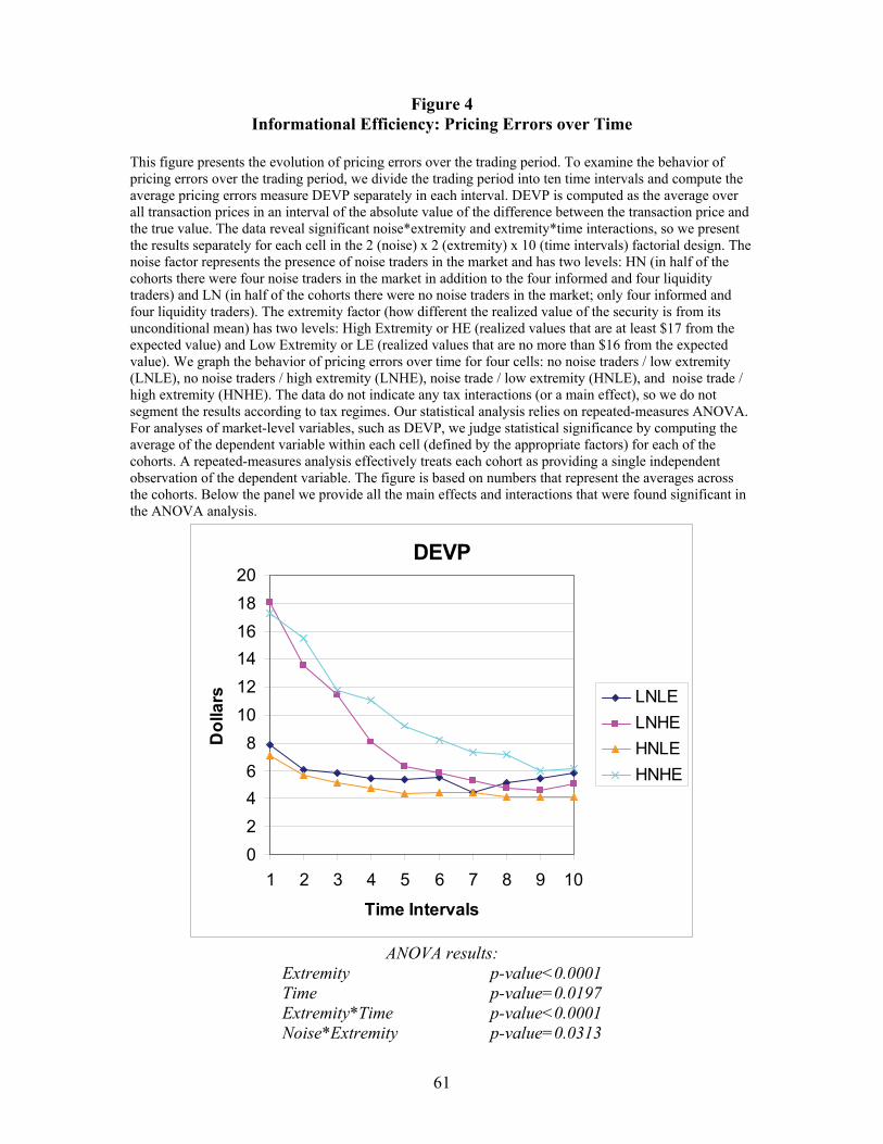
Figure 4 Informational Efficiency: Pricing Errors over Time

This figure presents the evolution of pricing errors over the trading period. To examine the behavior of pricing errors over the trading period, we divide the trading period into ten time intervals and compute the average pricing errors measure DEVP separately in each interval. DEVP is computed as the average over all transaction prices in an interval of the absolute value of the difference between the transaction price and the true value. The data reveal significant noise*extremity and extremity*time interactions, so we present the results separately for each cell in the 2 (noise) x 2 (extremity) x 10 (time intervals) factorial design. The noise factor represents the presence of noise traders in the market and has two levels: HN (in half of the cohorts there were four noise traders in the market in addition to the four informed and four liquidity traders) and LN (in half of the cohorts there were no noise traders in the market; only four informed and four liquidity traders). The extremity factor (how different the realized value of the security is from its unconditional mean) has two levels: High Extremity or HE (realized values that are at least $17 from the expected value) and Low Extremity or LE (realized values that are no more than $16 from the expected value). We graph the behavior of pricing errors over time for four cells: no noise traders / low extremity (LNLE), no noise traders / high extremity (LNHE), noise trade / low extremity (HNLE), and noise trade / high extremity (HNHE). The data do not indicate any tax interactions (or a main effect), so we do not segment the results according to tax regimes. Our statistical analysis relies on repeated-measures ANOVA. For analyses of market-level variables, such as DEVP, we judge statistical significance by computing the average of the dependent variable within each cell (defined by the appropriate factors) for each of the cohorts. A repeated-measures analysis effectively treats each cohort as providing a single independent observation of the dependent variable. The figure is based on numbers that represent the averages across the cohorts. Below the panel we provide all the main effects and interactions that were found significant in the ANOVA analysis.

DEVP

02468

101214161820

1 2 3 4 5 6 7 8 9 10

Time Intervals

Dol

lars LNLE

LNHEHNLEHNHE

ANOVA results:

Extremity p-value<0.0001 Time p-value=0.0197 Extremity*Time p-value<0.0001 Noise*Extremity p-value=0.0313

61

Figure 5 Trading Strategies: Taking Rates of Limit Orders

In this set of figures we present the taking rates of limit orders by the different trader types over the trading period. The Taking Rate is defined as the number of shares a trader trades by submitting market orders divided by the total number of shares he trades (where the denominator consists of both market and executed limit orders). The higher the taking rate, the more the trader transact by demanding rather than supplying liquidity. The Taking Rate also speaks to the aggressiveness or trading urgency (as apposed to patience) demonstrated by traders. To examine the behavior of the taking rate over the trading period, we divide the trading period into ten time intervals and compute the taking rate separately in each interval. The data reveal a significant type*time interaction, so we present the results separately for each cell in the (trader type) x (time intervals) factorial design. The trader type factor has three levels in half of the cohorts (informed traders, liquidity traders, and noise traders) and two levels in half of the cohorts (informed and liquidity traders only). The data do not indicate any tax or extremity interactions or main effects, so we do not segment the results according to these factors. We present two side-by-side figures: one for the cohorts without noise trader participation and one for the cohorts with noise traders. Our statistical analysis relies on repeated-measures ANOVA. For analyses of individual-level variables (such as the taking rate), we first compute the variable under investigation for an individual trader and then the average for a trade type within each of the cohorts. A repeated-measures analysis effectively treats each cohort as providing a single independent observation of the dependent variable. The numbers in the table represent the averages across the cohorts. Below the panel we provide all the main effects and interactions that were found significant in the ANOVA analysis.

ANOVA results of sessions w/o Noise Traders: Time p-value=0.0426 Type*Time p-value<0.0001

ANOVA results of sessions with Noise Traders: Time p-value=0.0049 Type p-value<0.0001 Type*Time p-value<0.0001

Taking Rate with Noise

0%10%20%30%40%50%60%70%80%

1 2 3 4 5 6 7 8 9 10

Time Intervals

InformedLiquidityNoise

Taking Rate w/o Noise

0%10%20%30%

40%50%60%70%

1 2 3 4 5 6 7 8 9 10

Time Intervals

InformedLiquidity

62