How Q and Cash Flow Affect Investment

without Frictions: An Analytic

Explanation1

Andrew B. Abel

The Wharton School of the University of Pennsylvania

National Bureau of Economic Research

Janice C. Eberly

Kellogg School of Management, Northwestern University

National Bureau of Economic Research

August 2008, current version November 2008

1Earlier versions of this paper circulated under the title “Q Theory without Adjustment

Costs & Cash Flow Effects without Financing Constraints.” We thank Joao Gomes, Philipp

Illeditsch, Richard Kihlstrom, Michael Michaux, Stavros Panageas, Julien Prat, and Ken

West for helpful comments, as well as seminar participants at the Federal Reserve Bank

of Kansas City, New York University, Stanford University, University of California at San

Diego, University of Chicago, University of Wisconsin, University of Southern California,

the Penn Macro Lunch Group, the Workshop on Firms’ Dynamic Adjustment in Bergamo,

Italy, and the Society for Economic Dynamics meeting in Florence, Italy.

Abstract

We derive a closed-form solution for Tobin’s Q in a stochastic dynamic framework.

We show analytically that investment is positively related to Tobin’s Q and cash flow,

even in the absence of adjustment costs or financing frictions. In the spirit Brainard

and Tobin (1968), shocks to firm growth move Q and investment together since both

increase with positive shocks to revenue growth. Similarly, shocks to current cash

flow, arising from shocks to the user cost of capital in our model, cause investment

and cash flow per unit of capital to comove positively. Furthermore, we show that

this alternative mechanism for the relationship among investment, Q, and cash flow

delivers larger cash flow effects for smaller and faster-growing firms, as observed in

the data. Moreover, the empirically small correlation between investment and Tobin’s

Q does not imply implausibly large adjustment costs in our model (since there are

no adjustment costs), but simply reflects a common response to changes in the firm’s

revenue growth.

Regressions of investment on Tobin’s Q and cash flow typically yield a small

positive coefficient on Q and a significant positive coefficient on cash flow. The small

coefficient on Q is interpreted as evidence of strongly convex adjustment costs, and

the significant cash flow coefficient is interpreted as evidence of the importance of

financing constraints facing firms. In this paper we develop and analyze an economic

model in which both of these interpretations are false. In particular, we develop a

simple neoclassical model without adjustment costs and without financing constraints.

We show analytically that the investment-capital ratio depends positively on Tobin’s

Q and on cash flow per unit of capital. The coefficient on Q can be small, yet it

cannot be interpreted as strongly convex adjustment costs, because adjustment costs

are excluded from model. The positive effect of cash flow on investment cannot

be interpreted as a reflection of financing constraints because there are no financing

constraints in the model. In our model, these effects arise because Tobin’s Q reflects

expectations about future revenue growth, while cash flow reflects the effects of the

user cost of capital. Since both of these underlying shocks (revenue growth and the

user cost of capital) drive investment, investment will be correlated with both Q and

cash flow.

James Tobin (1969) introduced the ratio of the market value of a firm to the

replacement cost of its capital stock — a ratio that he called “Q” — to measure the

incentive to invest in capital.1 Tobin’s Q, as it has become known, is the empirical

implementation of Keynes’s (1936) notion that capital investment becomes more at-

tractive as the value of capital increases relative to the cost of acquiring the capital.

Neither Keynes nor Tobin provided a formal decision-theoretic analysis underlying

the Q theory of investment. Lucas and Prescott (1971) developed a rigorous analysis

of the capital investment decision in the presence of convex costs of adjustment, and

observed that the market value of capital can be an important element of the capital

1Brainard and Tobin (1968) introduced the idea that a firm’s investment should be positively

related to the ratio of its market value to the replacement value of its capital stock, though they did

not use the letter Q to denote this ratio.

1

investment decision, though they did not explicitly make the link to Tobin’s Q.

The link between convex costs of adjustment and the Q theory of investment was

made explicitly by Mussa (1977) in a deterministic framework and by Abel (1983) in

a stochastic framework, though the papers based on convex adjustment costs focused

onmarginal Q — the ratio of the value of an additional unit of capital to its acquisition

cost — rather than the concept of average Q introduced by Tobin. Hayashi (1982)

bridged the gap between the concept of marginal Q dictated by the models based on

convex adjustment costs and the concept of average Q, which is readily observable,

by providing conditions, in a deterministic framework, under which marginal Q and

average Q are equal. Specifically, marginal Q and average Q are equal for a com-

petitive firm with a constant-returns-to-scale production function provided that the

adjustment cost function is linearly homogeneous in the rate of investment and the

level of the capital stock. Abel and Eberly (1994) extended Hayashi’s analysis to the

stochastic case and also analyzed the relationship between average Q and marginal

Q in some special situations in which these two variables are not equal.

In the current paper, we develop a new theoretical basis for the empirical rela-

tionship between investment and Q that differs from the literature based on convex

adjustment costs in two major respects. First, we will dispense with adjustment

costs completely, and assume that a firm can instantaneously and completely adjust

its capital stock by purchasing or selling capital at an exogenous price, without hav-

ing to pay any costs of adjustment. Second, average Q and marginal Q will differ

from each other. In the literature based on convex adjustment costs, when average

Q and marginal Q differ, it is marginal Q that is relevant for the investment decision,

which is unfortunate since average Q is more readily observable than marginal Q. In

the current paper, it is average Q that is related to the rate of investment; in fact,

marginal Q is identically equal to one in this model and hence it cannot be related

to fluctuations in investment.

Both averageQ and marginalQ would be identically equal to one for a competitive

firm with a constant-returns-to-scale production function that can purchase and sell

2

capital at an exogenous price without any cost of adjustment. In order for average

Q to exceed one, the firm must earn rents through the ownership or exploitation of a

scarce factor. In the traditional Q-theoretic literature, the convex adjustment cost

technology is the source of rents for a competitive firm with a constant-returns-to-

scale production function. In the current paper, which has no convex adjustment

costs, rents are earned as a result of monopoly power or as a result of decreasing

returns to scale in the production function. A contribution of this paper is to show

that not only do these rents cause average Q to exceed one, but that fluctuations in

average Q are positively related to fluctuations in the investment-capital ratio. Thus,

our mechanism for a “Q-theoretic” model remains in the spirit of Brainard and Tobin

since the present value of future rents is correlated with optimal investment; however,

we show that adjustment costs are not necessary to this finding.

Lindenberg and Ross (1981) derive the value of Tobin’sQ for a firm with monopoly

power that does not face convex costs of adjustment. They focus on the extent to

which Tobin’s Q provides a measure of, or at least a bound on, monopoly power. Un-

like our paper, they do not emphasize the link the between investment and Tobin’s Q.

More importantly, their analysis is conducted in a deterministic framework that does

not admit interesting time-series variation in Tobin’s Q.2 A major contribution of our

paper, relative to this earlier work, is that we embed the firm in a stochastic environ-

ment that is rich enough to generate interesting time-series variation in Tobin’s Q,

yet tractable enough to be used to derive a closed-form solution for Tobin’s Q. This

solution for Tobin’s Q, with interesting time-series variation, is a critical ingredient to

our study of the predicted effect on investment of a change in Tobin’s Q. Similarly,

Schiantarelli and Georgoutsos (1990) specify a model of investment with monopolistic

competition, but also allow for quadratic costs of adjusting capital. They show that

in addition to a richer dynamic structure,3 output enters the equation relating invest-

2Their footnote 9 outlines an extension to the stochastic case, but does not derive a closed-form

solution for Tobin’s Q that has interesting stochastic variation.3Future values of investment and Q enter the equation, in addition to the usual current value of

Tobin’s Q.

3

ment and Tobin’s Q. This gives a rationale for output to appear in the investment

equation, but the mechanism is distinct from the one that generates a cash flow effect

in this paper, since the mechanism here requires no adjustment costs at all.4

An important implication of traditional Q-theoretic models based on convex ad-

justment costs is that (marginal) Q is a sufficient statistic for the rate of investment.

Other variables should not have any additional explanatory for investment if Q is an

explanatory variable. However, many empirical studies of investment and Q have re-

jected this implication by finding that cash flow has a significant effect on investment,

even if Q is included as an explanatory variable. This finding has been interpreted

by Fazzari, Hubbard, and Petersen (1988) and others as evidence of financing con-

straints facing firms. In the model we develop here, there are no financing constraints

— capital markets are perfect — yet investment is positively related to cash flow in ad-

dition to Q. Investment and cash flow (per unit of capital) positively comove in

our model because both react in the same direction to shocks to the user cost of

capital. Furthermore, in our model this “cash flow effect” on investment is larger for

smaller and faster-growing firms, as has been found empirically; it is usually argued

that this differential cash flow effect across groups of firms strengthens the financing

constraints interpretation, but in this model these differential effects exist in perfect

capital markets.

The interpretation of cash flow effects as evidence of financing constraints is also

called into question by Gomes (2001); in his quantitative model, optimal investment

is sensitive to both Tobin’s Q and cash flow, whether or not a cost of external fi-

nance is present. Similarly, Cooper and Ejarque (2003) numerically solve a model

with quadratic adjustment costs and a concave revenue function, and also find that

4 In particular, because of the convex adjustment costs, marginal Q is the appropriate indicator

of investment in their model, but Tobin’s Q is observable and appears in the estimated investment

equation. The output-capital ratio appears in the estimated investment equation to correct for

mismeasurement; it proxies for the gap between (measured) Tobin’s Q and marginal Q. The

output-capital ratio therefore appears with a negative sign in their specification to capture the scale

of the firm, and hence the gap between marginal and average Q.

4

investment is sensitive to both Tobin’s Q and cash flow in the absence of financing

constraints. In addition, they find that adding a fixed cost of access to capital mar-

kets does not improve the fit of the model and they conclude the cash flow sensitivity

of investment reflects market power rather than financial constraints. Alti (2003) de-

velops a continuous-time model of a firm facing quadratic adjustment costs and with

a revenue function that is concave in the capital stock and subject to a multiplicative

productivity shock. The logarithm of the shock reverts to an unknown mean and

firms update their estimates of the mean by observing realizations of cash flow over

time. For young firms, the estimate of the mean is noisy and Tobin’s Q provides a

noisy measure of long-run prospects that are important for investment.5 For these

firms especially, observations on cash flow provide important evidence that can change

the estimate of the mean level of productivity and hence affect investment.6 Gomes

(2001), Cooper and Ejarque (2003), and Alti (2003) numerically compute Tobin’s Q

because they cannot analytically solve for the value of the firm. A contribution of our

current paper is that we provide a closed-form solution for the value of the firm and

hence for Tobin’s Q. The importance of the closed-form solution is that it allows a

straightforward analytic description of the statistical relationship among investment,

Tobin’s Q and cash flow.

The model we develop is designed to be as simple as possible, yet rich enough to

deliver interesting time-series variation in the investment-capital ratio, Tobin’sQ, and

the ratio of cash flow to the capital stock. Section 1 presents the firm’s net revenue

as an isoelastic function of its capital stock. The revenue function is subject to

5Similarly, Erickson and Whited (2000) find that when controlling for measurement error in a

flexible way, the evidence for a cash flow effect on investment disappears in their sample.6A related, but different, interchange has occurred between Kaplan and Zingales (1997, 2000)

and Fazzari, Hubbard, and Petersen (2000). Kaplan and Zingales have argued both empirically and

theoretically that the sensitivity of investment to cash flow is not a reliable indicator of the degree

of financial constraints. This interchange is distinct from the model presented here, since we have

assumed no financial constraints at all, yet investment is sensitive to cash flow. Empirical work by

Gomes, Yaron, and Zhang (2006) also finds no evidence of financing constraints facing firms.

5

stochastic shocks that change its growth rate at random points in time. The optimal

capital stock is derived in Section 1 and the consequent optimal rate of investment

is derived in Section 2. Section 3 derives the value of the firm and Tobin’s Q. The

relationship among the investment-capital ratio, Tobin’s Q, and the cash flow-capital

stock ratio is analyzed in Section 4, and the effects of firm size and growth on this

relationship are analyzed in Section 5. Concluding remarks are presented in Section

6.

1 The Decision Problem of the Firm

Consider a firm that uses capital, Kt, and labor, Nt, to produce nonstorable output,

Yt, at time t according to the production function

Yt = At

¡Kγ

t N1−γt

¢s(1)

where At is productivity at time t, 0 < s ≤ 1 is the degree of returns to scale (s = 1for constant returns to scale) and 0 < γ < 1. The inverse demand function for the

firm’s output is

Pt = htY− 1ε

t (2)

where ht > 0 and ε > 1 is the price elasticity of demand. At time t, the firm chooses

labor, Nt, to maximize revenue net of labor costs, Rt = PtYt −wtNt, where wt is the

wage rate at time t. It is straightforward, but tedious, to show that if the firm uses

6

the optimal amount of labor, Nt, then revenue net of labor costs is7

Rt = Z1−αt Kαt , (3)

where Zt ≡ χ1

1−α

µhtw

−(1−γ)s(1− 1ε)

t A1− 1

εt

¶ εε−εs+s

reflects productivity, the demand for

the firm’s output, and the wage rate, α ≡ γs(1−1ε)

1−(1−γ)s(1− 1ε)

> 0, and χ > 0 is a constant.

Since Zt is an isoelastic function of ht, At, and wt (with different, but constant elas-

ticities, with respect to these three variables), the growth rate of Zt is a weighted

average of the growth rates of ht, At, and wt, with the weights equal to the corre-

sponding elasticities. For a competitive firm with constant returns to scale (ε = ∞and s = 1), α = 1. However, if the firm has some monopoly power (ε < ∞) or ifit faces decreasing returns to scale (s < 1), then α < 1 and hence net revenue is a

strictly concave function of the capital stock. This concavity implies that firm will

earn positive rents. Henceforth, we confine attention to the case with α < 1.

The variable Zt is exogenous to the firm and follows a geometric Brownian motion

with a time-varying drift, μt, so

dZt

Zt= μtdt+ σdz. (4)

If the growth rate μt were constant over time, the future growth prospects for the

firm would always look the same, and, as we will show, there would be no time-series

variation in the expected present value of the firm’s future operating profits relative

to current operating profits (more precisely, the present value in equation (29) would

7Use the production function in equation (1) and the inverse demand function in equation (2)

to write net revenue as Rt = gtNνt − wtNt, where gt ≡ htA

1− 1ε

t Kγs(1− 1

ε)t and ν ≡ (1− γ) s

¡1− 1

ε

¢.

Differentiating this expression for Rt with respect toNt and setting the derivative equal to zero yields

νgtNν−1t = wt, which can be used to write net revenue as Rt =

1−νν wtNt = (1− ν) ν

ν1−νw

− ν1−ν

t g1

1−νt .

Substitute the definition of gt into the expression for Rt and use the definition of α to obtain

Rt = χhw−νt htA

1− 1ε

t

i 11−ν

Kαt where χ ≡ (1− ν) ν

ν1−ν . Use the fact that 1 − α =

1−s(1− 1ε)

1−ν to

rewrite the expression for Rt as Rt =

∙χ

11−α

³w−νt htA

1− 1ε

t

´ 1

1−s(1− 1ε)¸1−α

Kαt so Rt = Z1−αt Kα

t

where Zt ≡ χ1

1−α³w−νt htA

1− 1ε

t

´ εε−sε+s

.

7

be a constant multiple of contemporaneous Zt). To introduce some interesting, yet

tractable, variation in the firm’s growth prospects, we assume that the process for Zt

follows a regime-switching process8 in which a regime is defined by a constant value

of the drift μt. A regime remains in force, that is, the drift remains constant, for a

random length of time. A new regime, which is characterized by a new value of the

drift, arrives with constant probability λ ≥ 0. The new value of the drift is drawn

from an unchanging distribution F (eμ) with support in the interval [μL, μH ]. The

values of the drift are i.i.d. across regimes and are independent of the realizations of

the other stochastic processes in the model. The value of the firm is finite and is

increasing in contemporaneous operating profit for a given value of the capital stock

if

E

½1

r + λ− eμ¾> 0 (5)

and

E

½λ

r + λ− eμ¾< 1, (6)

where r is the discount rate of the firm.

Henceforth, we assume that the following condition holds.

Condition 1 r > μH.

Condition 1, along with the fact that λ ≥ 0, implies that equations (5) and (6) bothhold.

The firm can purchase or sell capital instantaneously and frictionlessly, without

any costs of adjustment, at a constant price that we normalize to one. Because there

are no costs of adjustment, we can use Jorgenson’s (1963) insight that the optimal

path of capital accumulation can be obtained by solving a sequence of static decision

8Eberly, Rebelo, and Vincent (2008) find an important role for regime-switching in empirical

investment equations. Specifically, they report that a “single-regime model ... cannot explain the

role of lagged investment in investment regressions” but “the performance of the model can be

greatly improved by a regime-switching component” for the exogenous stochastic process. (p. 11)

8

problems using the concept of the user cost of capital. With the price of capital

constant and equal to one, the user cost of capital, υt, is

υt ≡ r + δt, (7)

where δt is the depreciation rate of capital. We will discuss the stochastic properties

of δt later in this section. For the specific goal of studying the relationship between

investment and Tobin’s Q, we could simply assume that δt is constant. Variation in

δt will be useful when we examine the effect of cash flow on investment.

At time t the firm chooses the capital stock Kt to maximize operating profit, πt,

which equals net revenue less the user cost of capital

πt ≡ Rt − υtKt = Z1−αt Kαt − υtKt. (8)

Differentiating equation (8) with respect to Kt and setting the derivative equal to

zero yields the optimal value of the capital stock

Kt = Zt (υt/α)−11−α . (9)

Substituting the optimal capital stock from equation (9) into equations (8) and (3),

respectively, yields the optimal level of operating profit

πt = (1− α)Zt (υt/α)−α1−α (10)

and the optimal level of revenue (net of labor cost)

Rt =1

1− απt. (11)

Empirical investment equations often use a measure of cash flow, normalized by

the capital stock, as an explanator of investment. Since Rt is defined as revenue net

of labor costs, it is cash flow before investment expenditure. Let ct ≡ Rt/Kt be the

cash flow before investment, normalized by the capital stock, and note, for later use,

that

ct =1

1− α

πtKt=

υtα, (12)

9

where the first equality follows from equation (11) and the second equality follows

from equations (9) and (10).

Equations (10) and (11) together imply that an increase in the user cost of capital,

υt, reduces cash flow, Rt. Although cash flow falls in response to an increase in the

user cost of capital, it does not fall by as much as the capital stock falls. Therefore, an

increase in the user cost of capital will increase cash flow per unit of capital. Indeed,

equation (12) indicates that cash flow per unit of capital is proportional to the user

cost of capital.

It will be convenient to define a variableMt that summarizes the effect of the user

cost on the optimal capital stock and operating profit, and to specify the stochastic

variation in Mt directly. In particular, define

Mt ≡³υtα

´ −α1−α

=

µr + δtα

¶ −α1−α

. (13)

We assume that Mt is a martingale and is independent of the parameters and real-

izations of the process for Zt. The assumption that Mt is a martingale implies that

δt is not a martingale. In particular, it implies that the depreciation rate is expected

to grow over time.9 For the sake of concreteness, we assume that Mt is a trendless

9Note that for τ > 0, 1 = Et

nMt+τ

Mt

o= Et

½³υt+τυt

´− α1−α

¾>hEt

nυt+τυt

oi− α1−α, where the

first equality follows from the assumption that Mt is a martingale, the second equality follows

from the definition of Mt, and the third (in)equality follows from Jensen’s inequality. Therefore,

Et

nυt+τυt

o> 1, which implies that Et {δt+τ} > δt so that the depreciation rate is expected to

grow over time. This implication is consistent with depreciation rates computed for U.S. private

nonresidential fixed assets using the Bureau of Economic Analysis Fixed Asset Tables 4.1 and 4.4 and

taking the ratio of annual depreciation to the beginning-of-year net stock of capital. The average

depreciation rates for 1950-59, 1970-79, and 1997-2006 are, respectively, 6.3%, 7.1%, and 8.2%. For

equipment and software, the corresponding figures are 13.7%, 14.2%, and 16.8%, and for structures

the corresponding figures are 2.8%, 3.0% and 3.0%.

10

geometric Brownian motion. Specifically, we assume that10

dMt = σMMtdzM , (14)

where σM > 0.

Use the definition ofMt in equation (13) to rewrite the expressions for the optimal

capital stock and the optimal operating profit in equations (9) and (10), respectively,

as

Kt = ZtM1αt (15)

and

πt = (1− α)ZtMt. (16)

Equations (15), (16) and (11) indicate that the capital stock, operating profit, and

revenue are all increasing functions of contemporaneous values of Zt and Mt and are

independent of μt, conditional on Zt and Mt. Thus, regardless of whether firm size

is measured by the size of the capital stock, operating profit, or revenue, firm size is

increasing in Zt and Mt, but is independent of μt. In addition, equations (15) and

(16) imply that πtKt= (1− α)M

− 1−αα

t so that πtKtis a decreasing funtion of Mt and

hence πtKtis larger for small firms than for large firms.

In Section 2 we examine the firm’s investment by analyzing the evolution of the

optimal capital stock in equation (15). Then in Section 3 we use the expression for

the optimal operating profit in equation (16) to compute the value of the firm.

2 Investment

Gross investment is the sum of net investment, dKt, and depreciation δtKtdt. To

calculate net investment divided by the capital stock, apply Ito’s Lemma to the

expression for the optimal capital stock in equation (15) and use the processes for Zt

10Although the process in equation (14) implies that if the initial value of Mt is positive, it will

remain positive, it does not ensure that δt is positive (it implies that δt > −r).

11

and Mt in equations (4) and (14), respectively, to obtain

dKt

Kt= μtdt+

1

2

1− α

α2σ2Mdt+ σdz +

1

ασMdzM . (17)

Adding the depreciation rate of capital, δt, to net investment per unit of capital in

equation (17) yields gross investment per unit of capital

dItKt≡ dKt

Kt+ δtdt = (μt + δt) dt+

1

2

1− α

α2σ2Mdt+ σdz +

1

ασMdzM . (18)

Investment is a linear function of the growth rate, μt, the depreciation rate, δt,

and a mean-zero disturbance, σdz + 1ασMdzM , that is independent of μt and δt. If

μt and δt, as well as the investment-capital ratio, were observable, then we could use

a linear regression to estimate the effects on the investment-capital ratio of μt and

δt. In a sufficiently large sample, the coefficients on μt and δt would both equal one.

However, μt is not observable and δt may not be well measured. We will show in

later sections that movements in μt are reflected by movements in Tobin’s Q, and

movements in δt are reflected by movements in the firm’s cash flow per unit of capital

and in Tobin’s Q. Thus, Tobin’s Q and cash flow per unit of capital can help to

explain investment statistically.

3 The Value of the Firm and Tobin’s Q

The value of the firm, Vt, is the present value of current and expected future cash

flows, net of the cost of current and future investment, and satisfies

rVtdt = Et {Rtdt− (dKt + δtKtdt) + dVt} . (19)

The left hand side of equation (19) is the required return on the firm over the interval

of time from t to t + dt, and the right hand side of equation (19) is the expected

return over this interval of time. The expected return on the right hand side consists

of two components: (1) the expected net cash flow, which equals revenue, Rt, less

gross investment dKt+ δtKtdt and (2) the expected capital gain or loss reflecting the

change in the value of the firm.

12

The value of the firm depends on three state variables11 — Zt, Mt, and μt — so

the value of the firm in equation (19) can be written as Vt = V (Zt,Mt, μt). To

express equation (19) in terms of the state variables, first use equations (11) and (16)

to obtain

Rt = ZtMt, (20)

and use equations (15) and (18) to obtain

Et {dKt + δtKtdt} =µμt + δt +

1

2

1− α

α2σ2M

¶ZtM

1αt dt. (21)

Then, to calculate dV (Zt,Mt, μt), use Ito’s Lemma, equations (4) and (14) for the

evolution of Zt and Mt, respectively, and the stochastic process for μt to obtain

Et {dV (Zt,Mt, μt)} = VZμtZtdt+1

2VZZσ

2Z2t dt+1

2VMMσ2MM2

t dt (22)

+λ [Et {V (Zt,Mt, eμ)− V (Zt,Mt, μt)}] dt.

Equations (20), (21), and (22) allow us to rewrite equation (19) as

rV (Zt,Mt, μt) = ZtMt −µμt + δt +

1

2

1− α

α2σ2M

¶ZtM

1αt + VZμtZt (23)

+1

2VZZσ

2Z2t +1

2VMMσ2MM2

t + λ [Et {V (Zt,Mt, eμ)− V (Zt,Mt, μt)}] .

In Appendix B, we show that a solution to equation (23) is

V (Zt,Mt, μt) = ZtM1αt +

ω (1− α)ZtMt

r + λ− μt(24)

where12

ω ≡∙E

½r − eμ

r + λ− eμ¾¸−1

≥ 1, (25)

with strict inequality if λ > 0.

Here we present a heuristic derivation of the value function that has a simple

economic interpretation. The value of the firm can be derived by viewing the firm as

11The capital stock is instantaneouly and costlessly adjustable so it is not a state variable.12Since ω−1 = E

nr−μ

r+λ−μo= 1 − E

nλ

r+λ−μo, equation (5) implies that ω−1 ≤ 1, with strict

inequality if λ > 0, and equation (6) implies that ω−1 > 0. Therefore, since 0 < ω−1 ≤ 1, ω ≥ 1,with strict inequality if λ > 0.

13

composed of two divisions — a capital-owning division that owns Kt at time t and a

capital-operating division that produces and sells output at time t. Because capital

can be instantaneously and costlessly bought or sold at a price of one at time t, the

value of the capital-owning division at time t isKt. The value of the capital-operating

division, which rents capital (in an amount equal to the amount of capital owned by

the capital-owning division) to produce and sell output, is the present value of current

and expected future operating profits. Therefore, the value of the firm at time t is

Vt = Kt +Et

½Z ∞

t

πt+τe−rτdτ

¾. (26)

As a step toward calculating the present value in equation (26), use equation (16),

the independence of Mt and Zt, and the fact that Mt is a martingale to obtain

Et {πt+τ} = (1− α)MtEt {Zt+τ} . (27)

Substituting equation (27) into equation (26) yields

Vt = Kt + (1− α)Mt

Z ∞

t

Et {Zt+τ} e−rτdτ. (28)

We show in Appendix A that the value of the integral on the right hand side of

14

equation (28) is13 ,14 Z ∞

t

Et {Zt+τ} e−rτdτ = ω

r + λ− μtZt. (29)

Note that when the arrival rate λ is zero, so that the growth rate of Zt remains μt

forever, ω = 1 and the expected present value of the stream of Zt+τ in equation (29)

is simply Zt/ (r − μt). More generally, when the growth rate μt varies over time, a

high value of μt implies a high value of the present value in equation (29).

The value of the firm can now be obtained by substituting equation (29) into

equation (28), and recalling from equation (16) that πt = (1− α)ZtMt, to obtain

Vt = Kt +ωπt

r + λ− μt. (30)

Equation (30) is equivalent to equation (24) because equation (15) states that Kt =

ZtM1αt and equation (16) states that πt = (1− α)ZtMt.

13To derive the present value of Zt+τ heuristically, let Pt = P (μt, Zt) ≡R∞t

Et {Zt+τ} e−rτdτ bethe price of a claim on the infinite stream of Zt+τ for τ ≥ 0. The expected return on this claim

over an interval dt of time is Ztdt + Et{dPt}. Because the path of future growth rates of Zt is

independent of the current value of Zt, P (μt, Zt) can be written as p (μt)Zt. The expected change

in Pt is Et {dPt} = λZt [p∗ − p (μt)] dt+ μtZtp (μt) dt, where p

∗ is the unconditional expectation of

p (μt) so the first term is the expected change arising from a new drawing of the growth rate μt, and

the second term reflects the fact (from equation 4) that Et {dZt} = μtZtdt. Setting the expected

return equal to the required return rp (μt)Ztdt, and solving yields (r + λ− μt) p (μt) = 1 + λp∗.

Therefore,

p (μt) =1 + λp∗

r + λ− μt.

Taking the unconditional expectation of both sides of this expression yields p∗ =

(1 + λp∗)En

1r+λ−μ

o, which can be rearranged to obtain p∗ = ωE

n1

r+λ−μosince ω ≡h

En

r−μr+λ−μ

oi−1. Therefore 1 + λp∗ = ω, so p (μt) =

ωr+λ−μt .

14As we show in footnote 13, ω = 1+λp∗ where p∗ > 0 because it is the present value of a stream

of positive variables. Therefore, ω ≥ 1, with strict inequality if λ > 0. Also from footnote 13,

p∗ = ωEn

1r+λ−μ

o> 0. As we show in footnote 12, equations (5) and (6) together imply that

ω ≥ 1, and equation (5) then is needed for p∗ > 0.

15

3.1 Tobin’s Q

Tobin’s Q is the ratio of the value of the firm to the replacement cost of the firm’s

capital stock. Since the price of capital is identically equal to one, the replacement

cost of the firm’s capital stock is simplyKt. Dividing the value of the firm in equation

(30) by Kt yields

Qt ≡ VtKt= 1 +

ω

r + λ− μt

πtKt

> 1. (31)

Tobin’s Q is greater than one because the firm earns rents πt. In the absence of

rents, Tobin’s Q would be identically equal to one because the firm can costlessly and

instantaneously purchase and sell capital at a price of one.15

The presence of positive rents πt is sufficient to make Tobin’s Q greater than one

in our model. However, rents alone do not imply that Tobin’s Q will vary over time

for a firm. If Zt were to grow at constant rate, so that μt were constant, and if the

user cost υt were constant, so that πtKtwere constant (see equation 12), then equation

(31) shows that Tobin’s Q would be constant and greater than one.16 However, we

have modeled both the growth rate μt and the user cost υt as stochastic, and equation

(31) shows that Tobin’s Q is an increasing function of the contemporaneous growth

rate μt and an increasing function of the contemporaneous value of operating profit

per unit of capital (which is proportional to cash flow per unit of capital). Recall

from the discussion following equations (15) and (16) that πtKtis higher for small firms

than for large firms. Therefore, the value of Qt in equation (31) is higher for small

firms than for large firms.

This effect of the growth rate μt on Qt illustrates the distinction in the finance

15Sargent (1980) presents a model without convex adjustment costs in which Tobin’s Q can differ

from one. In Sargent’s model, Tobin’s Q can never exceed one because firms are competitive and do

not earn rents, and they can always acquire additional capital instantly at a price of one. However,

because investment is irreversible in Sargent’s model, Tobin’s Q can fall below one.16Thus, decreasing returns to scale or market power, as in Alti (2003) and Cooper and Ejarque

(2001) are not sufficient to generate our results. Those papers generate time variation in rents with

adjustment costs, whereas we allow time variation in growth prospects and eliminate adjustment

costs.

16

literature between growth stocks and value stocks. Value stocks are identified as

stocks with high book-to-market ratios, that is, stocks with low values of Qt. By

contrast, growth stocks are those with high values of Qt, which is consistent with

equation (31) because an increase in the expected growth rate μt increases the right

hand side of this equation.

4 The Effects of Tobin’s Q and Cash Flow on In-

vestment

Define ιt to be the predictable component of the investment-capital ratio at time t in

equation (18), so that, ignoring the constant 121−αα2

σ2M ,

ιt = μt + δt. (32)

However, the growth rate μt is not observable and the depreciation rate δt may not

be well measured. In this section, we show that the growth rate μt can be written as

a function of Tobin’s Q and cash flow per unit of capital ct, and that the depreciation

rate δt is related to cash flow ct. Thus, to the extent that Qt and ct reflect μt and

δt, these variables can help account for movements in investment.

First, we show that the growth rate μt can be expressed in terms of the observable

variables Qt and ct. Use equation (12) to substitute (1− α) ct for πtKtin equation

(31) to obtain

Qt = 1 + (1− α)ωct

r + λ− μt. (33)

Multiply both sides of equation (33) by r+λ−μt and rearrange to obtain an expressionfor the growth rate μt in terms of the observable values of Tobin’s Q and cash flow

normalized by the capital stock

μt = r + λ− (1− α)ωct

Qt − 1 . (34)

To express ιt = μt + δt as a function of Qt and ct, add δt to both sides of equation

(34), and use the fact from equation (12) that αct = υt and the definition of the user

17

cost υt ≡ r + δt to obtain

ι (Qt, ct) ≡µα− (1− α)ω

Qt − 1¶ct + λ. (35)

We will analyze the effects of Qt and ct on investment by analyzing the effects of these

variables on ι (Qt, ct).

First we analyze the effect of Tobin’s Q on investment for a given level of cash

flow ct. Let βQ ≡ ∂ι (Qt, ct) /∂Qt denote the response of the investment-capital ratio

to an increase in Qt. Partially differentiating ι (Qt, ct) with respect to Qt yields

βQ ≡∂ι (Qt, ct)

∂Qt=(1− α)ωct

(Qt − 1)2> 0, (36)

so that investment is an increasing function of Qt. The positive relationship between

investment and Tobin’s Q has some remarkable differences from the relationship in

the standard convex adjustment cost framework. The positive relationship between

investment and Qt arises in the standard framework because of the convexity of the

adjustment cost function. For instance, in the special case in which the adjustment

cost function is quadratic in investment, the relationship between investment and Q

is linear. In that case, in a regression of the investment-capital ratio on Qt and

ct, the coefficient on Qt is the reciprocal of the second derivative of the adjustment

cost function with respect to investment.17 This estimated coefficient, which is the

analogue of βQ in equation (36), is typically quite small, which is usually interpreted to

mean that adjustment costs are very large. In the model we present here, investment

is positively related to Qt, that is, βQ > 0, even though there are no convex costs of

adjustment. In addition, it is quite possible for βQ to be small (if (1− α)ωct is small

or if Qt is large). Yet, in this model, without convex adjustment costs, the small

value of βQ cannot indicate large adjustment costs, as in standard interpretations.

17In the case with adjustment costs that are quadratic in investment, and linearly homogenous in

investment and the capital stock, so that the optimal investment-capital ratio is a linear function

of Qt, the adjustment cost function C(It,Kt) can be written as C(It,Kt) =12b³ItKt

´2Kt. The

coefficient on Qt in an investment regression is 1b in this case. A small value of this coefficient

implies that b is large.

18

Another remarkable difference from standard models based on convex capital ad-

justment costs is that the investment-capital ratio is related to average Q, VtKt, rather

than to marginal Q, ∂Vt∂Kt, which equals one in this model.18 The relationship be-

tween investment and average Q in our model is noteworthy because average Q is

observable, whereas marginal Q is not observable. The link between investment and

Tobin’s Q arises here because, even in the absence of adjustment costs, investment is

a dynamic phenomenon. That is, investment is the growth of the capital stock plus

depreciation, and the growth of the optimal capital stock depends on μt, the growth

rate of Zt. Since Qt also depends on μt, it contains information about the growth of

the capital stock.

Another difference from the standard Q-theoretic framework based on convex

adjustment costs is that the relationship between investment and Q in our framework

is not structural. In the presence of convex adjustment costs, the relation between

investment and (marginal) Q is structural in the sense that it is a direct consequence

of the first-order condition equating the marginal cost of adjustment and marginal Q.

However, in the present framework, without convex adjustment costs, the relationship

between investment and Tobin’sQ is not structural. As emphasized by Sargent (1980)

in a different framework without convex adjustment costs, the relationship between

investment and Q does not represent any particular underlying cost or preference

function, and is sensitive to the stochastic properties of various variables.

Equation (35) has another remarkable feature. Even after taking account of

Qt on the rate of investment, investment also depends on normalized cash flow ct.

Empirical studies of investment often find that the firm’s cash flow per unit of capital

is positively related to the rate of investment per unit of capital, even when a measure

ofQ is included as an explanator of investment. A typical empirical equation, starting

from Fazzari, Hubbard, and Petersen (1988), would have the investment-capital ratio

as the dependent variable, and Tobin’s Q and ct, the ratio of the firm’s cash flow

18Caballero and Leahy (1996) and Abel and Eberly (1998) analyze optimal investment in the

presence of a fixed cost of investment and find that investment is related to average Q.

19

to its capital stock, as the dependent variables. The finding of a positive cash flow

effect is often interpreted as evidence of a financing constraint facing the firm.

To analyze the effect of cash flow on investment in our model, let βc ≡ ∂ι(Qt,ct,)∂ct

denote the response of the investment-capital ratio to an increase in cash flow per

unit of capital, ct, holding Tobin’s Q constant. Partially differentiate equation (35)

with respect to ct to obtain

βc ≡∂ι (Qt, ct)

∂ct= α− (1− α)ω

Qt − 1 . (37)

The sign of βc in equation (37) depends on the magnitudes of two competing

factors. Since r + δt = αct, a high value of ct indicates that δt is high and hence

that replacement investment as a fraction of the capital stock is high. This positive

effect of cash flow on the investment-capital ratio is captured by the first term, α, on

the right hand side of equation (37). Working in the opposite direction is the fact

that, for a given value of Qt, a high value of ct indicates a low value of the growth

rate μt because Qt is an increasing function of both ct and μt. The implied low value

of μt indicates a low growth rate of the capital stock and hence a low value of the

investment-capital ratio. This negative effect of cash flow on the investment-capital

ratio is captured by the second term, − (1−α)ωQt−1 , on the right hand side of equation

(37).

Use equation (33) to substitute (1−α)ωr+λ−μt ct for Qt−1 in equation (37), then use (12)

to substitute υtαfor ct, and use the definition of the user cost, υt ≡ r + δt, to obtain

the following the expression for βc

βc = αμt + δt − λ

r + δt. (38)

Condition 2 δt + μt > λ for all t.

Inspection of equation (38) reveals that Condition 2 is necessary and sufficient for

βc > 0.

Henceforth in this discussion we will assume that Condition 2 holds so that βc > 0;

note that the condition for a positive cash flow effect is most likely to hold for high

20

growth (high μt) firms. Although the traditional literature would interpret this

positive relationship between cash flow and investment as evidence of a financing

constraint, the positive effect arises in this model even though capital markets are

perfect and there are no financing constraints. A positive cash flow effect on in-

vestment in the absence of financing constraints undermines the logical basis for the

common tests of financing constraints in the literature.

The positive time-series relationship between investment and cash flow for a given

firm operates through the user cost of capital, υt. As we discussed in Section 2, an

increase in υt arising from an increase in the depreciation rate, δt, will increase gross

investment relative to the capital stock. As is evident from equation (12), an increase

in υt also increases the ratio of cash flow to the capital stock. Thus, the positive

time-series association between cash flow and investment reflects the fact that each

of these variables moves in the same direction in response to an increase in the user

cost of capital.

5 The Effects of Firm Size and Growth on the

Cash Flow Effect

The empirical literature on investment has found that cash flow has a more signifi-

cant positive effect on investment for firms that are small or growing quickly. This

finding has been interpreted as evidence that these firms face binding financial con-

straints, while large, slowly growing firms are either less constrained or financially

unconstrained. This conclusion is perhaps appealing because it coheres well with

the notion that small or rapidly growing firms do not have as much access to capital

markets and external financing as large, slowly growing firms have. In this section

we show that in our model, the effect of cash flow on investment, measured by βc,

is larger for firms that are small or rapidly growing than for large, slowly growing

firms, which is consistent with empirical findings, even though there are no financial

constraints in our model.

21

Recall from Section 3.1 that small firms have higher Qt than do large firms. In-

spection of equation (37) reveals that the cash flow coefficient βc is increasing in Qt.

Therefore, the cash flow coefficient βc is higher for small firms than for large firms,

which is consistent with the empirical finding that cash flow effects are stronger for

smaller firms.

The empirical literature sometimes identifies fast-growing firms as firms likely

to face binding financing constraints and finds that these firms have larger cash flow

coefficients than slow-growing firms. Inspection of equation (38) reveals that the cash

flow coefficient βc is an increasing function of the growth rate μt, which is consistent

with the empirical findings. Again, our model without any financing constraints is

consistent with empirical findings that have been interpreted as evidence of financing

constraints.

6 Concluding Remarks

This paper presents a new explanation for the empirical time-series relationship be-

tween investment and Tobin’s Q. Traditional explanations of this relationship are

based on convex costs of adjusting the capital stock. In this paper, we have assumed

that there are no such adjustment costs that drive a wedge between the purchase price

of capital and the market value of installed capital. Instead, the wedge between the

market value of a firm and the replacement cost of its capital stock is based on rents

accruing to market power or to decreasing returns to scale in the production function.

The presence of these rents implies that Tobin’s Q exceeds one.

Beyond showing that Q exceeds one, we showed that the investment-capital ratio

is positively related to Tobin’s Q, which is a measure of average Q, rather than

to marginal Q, as in the convex adjustment cost literature. This departure from

the adjustment cost literature is particularly important because average Q is readily

observable, whereas marginalQ is not directly observable. In the empirical literature,

relatively small responses of investment to Q have been taken as evidence of large

22

adjustment costs; here there are no adjustment costs at all, and yet the response of

investment to Q can be small.

In addition to being consistent with a positive relationship between investment

and Tobin’s Q, the model in this paper can account for the positive effect of cash

flow on investment, even when Q is included as an explanator of investment. The

common interpretation of the positive cash flow effect on investment is that it is ev-

idence of financing constraints facing firms. However, the model in this paper has

perfect capital markets without financing constraints, and yet cash flow can have a

positive effect on investment, even after taking account of the effect of Q on invest-

ment. Therefore, contrary to the common interpretation, a positive cash flow effect

on investment need not be evidence of a financing constraint.

The empirical literature has recognized that the investment regression may be

misspecified or mismeasured, leading to spurious cash flow effects. One strategy to

address these potentially spurious effects is to split the sample into a priori financially

constrained and unconstrained firms. Typically, smaller and faster growing firms,

which are often classified a priori as financially constrained, are found to have larger

cash flow effects. The same pattern of cash flow effects emerges in our model, even

though there are no financing constraints in the model, which calls into question the

interpretation of the empirical findings.

The model in this paper is, by design, very simple and stylized. In order for the

ratio of cash flow to the capital stock to exhibit time-series variation, the user cost of

capital must vary over time, and we induced this variation by allowing the deprecia-

tion rate to vary stochastically. In order for Tobin’s Q to exhibit time-series variation

that is not perfectly correlated with contemporaneous cash flow per unit of capital,

we assumed that the growth rate of Zt varies stochastically over time according to a

regime-switching model. We eliminated adjustment costs from the current analysis,

not because we believe they are irrelevant for an empirical investment model, but

rather because they are extraneous to the effects we examine here. The goal of the

current paper is to articulate the relationship among investment, Tobin’s Q, and cash

23

flow. Empirical findings regarding these relationships have been used to detect the

presence of adjustment costs and financing constraints, and to evaluate their impor-

tance for investment. Even when these adjustment costs and financing constraints

are eliminated, however, we show that investment remains sensitive to both Tobin’s Q

and cash flow, undermining traditional interpretations of empirical investment equa-

tions. Recent work using numerical modelling (Gomes (2001), Cooper and Ejarque

(2003), Eberly, Rebelo, and Vincent (2008)) has cast doubt on whether cash flow

effects identify financing constraints. That work shows quantitatively that such ef-

fects can arise with perfect capital markets in an empirically misspecified Q-theoretic

model (with adjustment costs). We show analytically that adjustment costs are not

necessary to generate a relationship between investment and Q, since rents may arise

and importantly, change over time, as the firm’s growth rate varies stochastically.

Moreover, cash flow effects still arise in this framework, since cash flow moves with

the user cost of capital, and hence with investment. Our results show in closed form

not only the difficulty of interpreting investment regressions in terms of adjustment

costs and financing frictions, but also provide a closed-form alternative interpretation

in terms of the firm’s growth prospects and the user cost of capital.

An avenue for future research would be to introduce richer and more realistic

processes for the various exogenous variables facing the firm. Another direction

would be to introduce delivery or gestation lags in the capital investment process.

In ongoing research (Abel and Eberly, 2005), we endogenize the growth in technol-

ogy, summarized here by an exogenous parameter, and similar effects arise in that

framework.

24

References

[1] Abel, Andrew B., “Optimal Investment Under Uncertainty,”

American Economic Review, 73:1 (March 1983), 228-233.

[2] Abel, Andrew B. and Janice C. Eberly, “A Unified Model of Investment Under

Uncertainty,” American Economic Review, 84:5 (December 1994), 1369-1384.

[3] Abel, Andrew B. and Janice C. Eberly, “The Mix and Scale

of Factors with Irreversibility and Fixed Costs of Investment,”

Carnegie-Rochester Conference Series on Public Policy, 48 (1998), 101-135.

[4] Abel, Andrew B. and Janice C. Eberly, “Investment, Valuation, and Growth

Options,” revised October 2005.

[5] Alti, Aydogan, “How Sensitive is Investment to Cash Flow When Financing is

Frictionless?” The Journal of Finance, 58, 2 (April 2003), 707-722.

[6] Brainard, William and James Tobin, “Pitfalls in Financial Model Building,”

American Economic Review, 58:2, (May 1968), pp. 99-122.

[7] Caballero, Ricardo and John V. Leahy, “Fixed Costs: The Demise of Marginal

q,” National Bureau of Economic Research Working Paper No. W5508, March

1996.

[8] Cooper, Russell and Joao Ejarque, “Financial Frictions and Investment: Re-

quiem in Q,” Review of Economic Dynamics, Vol. 6 (2003), 710-728.

[9] Eberly, Janice, Sergio Rebelo and Nicolas Vincent, "Investment and Value: A

Neoclassical Benchmark," National Bureau of Economic ResearchWorking Paper

No. 13866, March 2008.

[10] Erickson, Timothy and Toni M. Whited, “Measurement Error and the Relation-

ship between Investment and ‘q’,” Journal of Political Economy, Vol. 108, No.

5. (Oct., 2000), 1027-1057.

25

[11] Fazzari, Steven, R. Glenn Hubbard and Bruce Petersen, “Finance Constraints

and Corporate Investment,” Brookings Papers on Economic Activity, 1:1988,

141-195.

[12] Fazzari, Steven, R. Glenn Hubbard and Bruce Petersen, “Investment-Cash

Flow Sensitivities Are Useful: A Comment on Kaplan and Zingales,”

Quarterly Journal of Economics, 115:2 (May 2000), 695-706.

[13] Gomes, Joao F., “Financing Investment,” American Economic Review, 91:5 (De-

cember 2001), 1263-1285.

[14] Gomes, Joao F., Amir Yaron, and Lu Zhang, “Asset Pricing Implications of

Firms’ Financing Constraints,” Review of Financial Studies, 19:4 (Winter 2006),

1321-1356.

[15] Jorgenson, Dale W., “Capital Theory and Investment Behavior,”

American Economic Review, Papers and Proceedings, 53:2 (May 1963),

247-259.

[16] Kaplan, Steven N. and Luigi Zingales, “Do Investment-Cash Flow

Sensitivities Provide Useful Measures of Financing Constraints?”

Quarterly Journal of Economics, 112:1 (February 1997), 141-168.

[17] Kaplan, Steven N. and Luigi Zingales, “Investment-Cash Flow Sensitivities Are

Not Valid Measures of Financing Constraints,” Quarterly Journal of Economics,

115:2 (May 2000), 707-712.

[18] Keynes, JohnMaynard, The General Theory of Employment, Interest, and Money,

The Macmillian Press, Ltd., 1936.

[19] Lindenberg, Eric B. and Stephen A. Ross, “Tobin’s Q Ratio and Industrial Or-

ganization,” The Journal of Business, Vol. 54, No. 1. (Jan., 1981), 1-32.

[20] Lucas, Robert E., Jr. and Edward C. Prescott, “Investment Under Uncertainty,”

Econometrica, 39:5 (September 1971), 659-681.

26

[21] Mussa, Michael, “External and Internal Adjustment Costs and the Theory of

Aggregate and Firm Investment,” Economica, 44:174 (May 1977), 163-178.

[22] Sargent, Thomas J., “‘Tobin’s q’ and the Rate of Investment in Gen-

eral Equilibrium,” Carnegie-Rochester Conference Series on Public Policy, 12

(Spring 1980), 107-154.

[23] Schianterelli, Fabio, and G. Georgoutsos, ”Monopolistic Competition and the

Q Theory of Investment,” European Economic Review, 34:5 (July 1990), 1061-

1078.

[24] Tobin, James, “A General Equilibrium Approach to Monetary Theory,”

Journal of Money, Credit, and Banking, 1:1 (February 1969), 15-29.

27

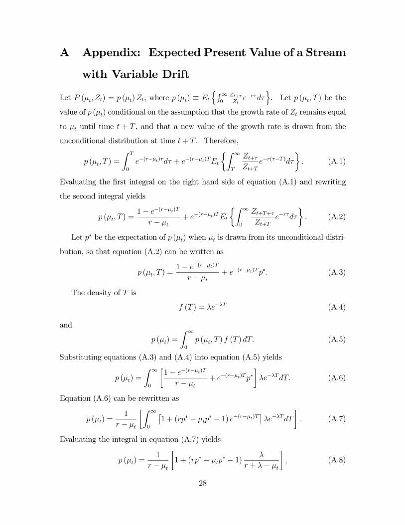
A Appendix: Expected Present Value of a Stream

with Variable Drift

Let P (μt, Zt) = p (μt)Zt, where p (μt) ≡ Et

nR∞0

Zt+τZt

e−rτdτo. Let p (μt, T ) be the

value of p (μt) conditional on the assumption that the growth rate of Zt remains equal

to μt until time t + T , and that a new value of the growth rate is drawn from the

unconditional distribution at time t+ T . Therefore,

p (μt, T ) =

Z T

0

e−(r−μt)τdτ + e−(r−μt)TEt

½Z ∞

T

Zt+τ

Zt+Te−r(τ−T )dτ

¾. (A.1)

Evaluating the first integral on the right hand side of equation (A.1) and rewriting

the second integral yields

p (μt, T ) =1− e−(r−μt)T

r − μt+ e−(r−μt)TEt

½Z ∞

0

Zt+T+τ

Zt+Te−rτdτ

¾. (A.2)

Let p∗ be the expectation of p (μt) when μt is drawn from its unconditional distri-

bution, so that equation (A.2) can be written as

p (μt, T ) =1− e−(r−μt)T

r − μt+ e−(r−μt)Tp∗. (A.3)

The density of T is

f (T ) = λe−λT (A.4)

and

p (μt) =

Z ∞

0

p (μt, T ) f (T ) dT. (A.5)

Substituting equations (A.3) and (A.4) into equation (A.5) yields

p (μt) =

Z ∞

0

∙1− e−(r−μt)T

r − μt+ e−(r−μt)Tp∗

¸λe−λTdT. (A.6)

Equation (A.6) can be rewritten as

p (μt) =1

r − μt

∙Z ∞

0

£1 + (rp∗ − μtp

∗ − 1) e−(r−μt)T ¤λe−λTdT¸ . (A.7)

Evaluating the integral in equation (A.7) yields

p (μt) =1

r − μt

∙1 + (rp∗ − μtp

∗ − 1) λ

r + λ− μt

¸, (A.8)

28

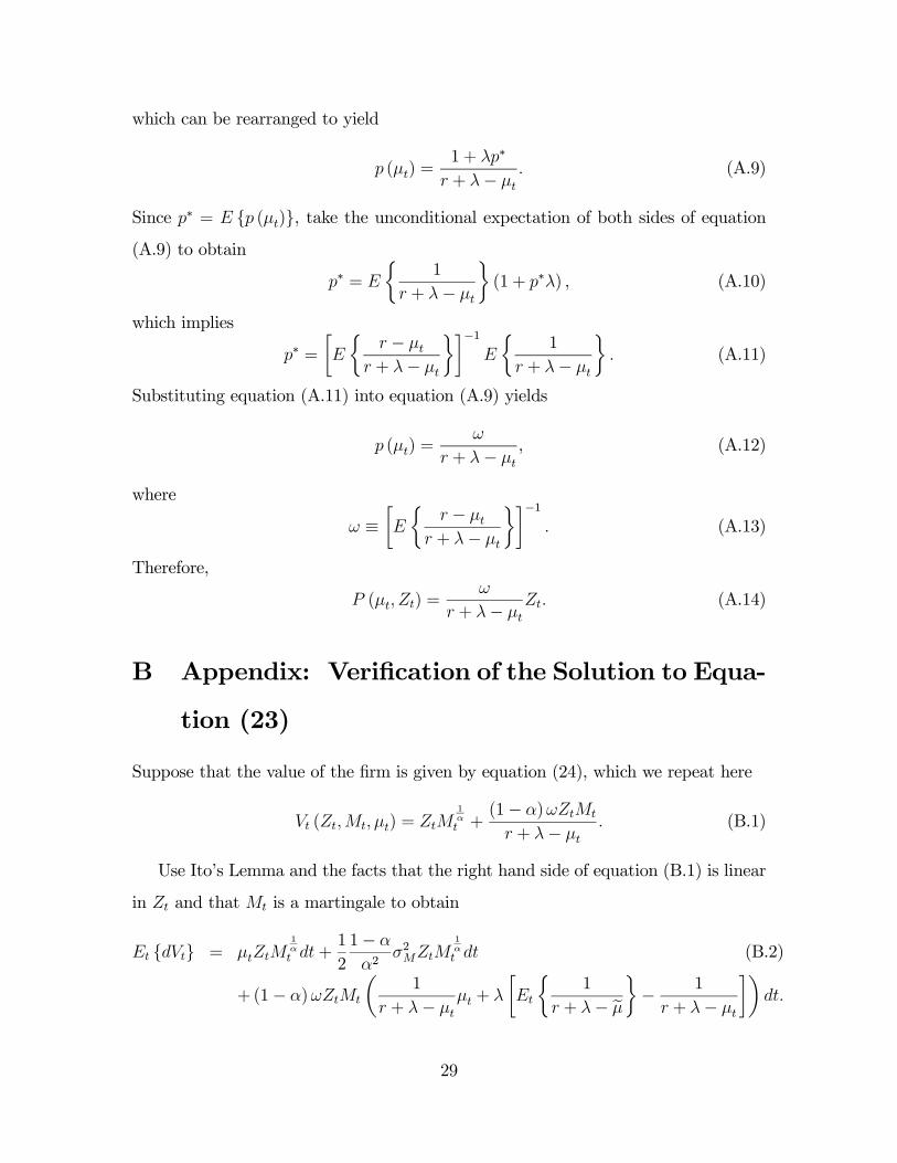
which can be rearranged to yield

p (μt) =1 + λp∗

r + λ− μt. (A.9)

Since p∗ = E {p (μt)}, take the unconditional expectation of both sides of equation(A.9) to obtain

p∗ = E

½1

r + λ− μt

¾(1 + p∗λ) , (A.10)

which implies

p∗ =∙E

½r − μt

r + λ− μt

¾¸−1E

½1

r + λ− μt

¾. (A.11)

Substituting equation (A.11) into equation (A.9) yields

p (μt) =ω

r + λ− μt, (A.12)

where

ω ≡∙E

½r − μt

r + λ− μt

¾¸−1. (A.13)

Therefore,

P (μt, Zt) =ω

r + λ− μtZt. (A.14)

B Appendix: Verification of the Solution to Equa-

tion (23)

Suppose that the value of the firm is given by equation (24), which we repeat here

Vt (Zt,Mt, μt) = ZtM1αt +

(1− α)ωZtMt

r + λ− μt. (B.1)

Use Ito’s Lemma and the facts that the right hand side of equation (B.1) is linear

in Zt and that Mt is a martingale to obtain

Et {dVt} = μtZtM1αt dt+

1

2

1− α

α2σ2MZtM

1αt dt (B.2)

+(1− α)ωZtMt

µ1

r + λ− μtμt + λ

∙Et

½1

r + λ− eμ¾− 1

r + λ− μt

¸¶dt.

29

Use the facts that Et

nλ

r+λ−μo= 1 − Et

nr−μ

r+λ−μoand μt−λ

r+λ−μt = −1 +r

r+λ−μt to

rewrite equation (B.2) as

Et {dVt} = μtZtM1αt dt+

1

2

1− α

α2σ2MZtM

1αt dt (B.3)

+(1− α)ωZtMt

µr

r + λ− μt−Et

½r − eμ

r + λ− eμ¾¶

dt.

Use equation (B.3) along with equations (20) and (21) to obtain

Et {Rtdt− (dKt + δtKtdt) + dVt} =⎡⎣ ZtMt − δtZtM

1αt

+(1− α)ωZtMt

³r

r+λ−μt −Et

nr−μ

r+λ−μo´ ⎤⎦ dt.(B.4)

Use the definition of ω in equation (25) to substitute ω−1 for En

r−μr+λ−μ

oin equa-

tion (B.4) to obtain

Et {Rtdt− (dKt + δtKtdt) + dVt} =∙αZtMt − δtZtM

1αt +

r (1− α)ωZtMt

r + λ− μt

¸dt.

(B.5)

Add and subtract rZtM1αt on the right hand side of equation (B.5) to obtain

Et {Rtdt− (dKt + δtKtdt) + dVt} =⎡⎣ ³

αMt − (r + δt)M1αt

´Zt

+r³(1−α)ωZtMt

r+λ−μt + ZtM1αt

´⎤⎦ dt. (B.6)

Use the definition Mt ≡¡υtα

¢ −α1−α =

¡r+δtα

¢ −α1−α to show that

αMt − (r + δt)M1αt = 0. (B.7)

Substitute equation (B.7) into equation (B.6) to obtain

Et {Rtdt− (dKt + δtKtdt) + dVt} = r

µ(1− α)ωZtMt

r + λ− μt+ ZtM

1αt

¶dt. (B.8)

Finally, use equation (B.1) to rewrite the right hand side of equation (B.8) so that

Et {Rtdt− (dKt + δtKtdt) + dVt} = rVtdt,

which shows that equation (24) is a solution to equation (23).

30