How Responsive is Higher Education?

The Linkages between Higher Education and the Labor Market

Ashok Bardhana, Daniel L. Hicksb, and Dwight Jaffeea a Haas School of Business, University of California, Berkeley

b Department of Economics, University of Oklahoma

[ Preliminary: Do Not Cite ]

Abstract:

Innovation is often cited as a panacea for the continued competitiveness of the US economy, and the higher education sector is considered vital in developing the productive and dynamic labor force critical for sustaining this innovation. But how effectively does the higher education sector meet the needs of the labor market? We design a crosswalk to match IPEDS data on post-secondary degrees completed in the US between 1984 and 2006 with occupational employment statistics from the BLS and CPS. Analysis reveals a sizeable degree of heterogeneity and lag in the responsiveness of the higher education sector to the needs of industry across specific occupation-degree pairings. Failure to respond rapidly to changes in labor demand may be one factor driving inequality in wages across occupations and in the aggregate economy. We suggest some simple policy measures to help increase the responsiveness and supply elasticity of the higher education sector, both in terms of the output of specific degree programs and the overall mix and composition of graduate completions.

Acknowledgments: We are especially grateful to David Autor, Barry Hirsch, David Levine and Edward Miguel for their encouragement and suggestions. We would also like to thank seminar participants at the Sloan Industry Studies Conference 2009 for helpful comments and discussions.

Section I: Introduction and Motivation

The last decade has witnessed the emergence and rapid growth of services offshoring on

an international scale. Competition increasingly takes place not just between countries or firms,

but between individuals. The creation of a single global labor market means that competitive

pressures are being felt across a broader range of occupations and workers. Meanwhile, rapid

technological growth continues to dictate changes in the occupational mix. The changing nature

of competition coupled with an escalating premium on technological skills pose challenges for

continued domestic job creation. Accordingly, greater attention is being focused on the higher

education sector as a key factor in preparing a dynamic work force capable of coping with these

challenges. What kind of workers are needed and what kinds of jobs will be created? How must

the higher education sector be positioned so that it fulfills the needs of a labor market in constant

flux?

These developments have brought to the forefront concerns over competitiveness,

outsourcing, and skill biased technical change. While academic debate continues on many of

these issues, there has been a general agreement among researchers and pundits that innovation

and higher education are key policy responses to these mounting challenges. Significant attention

has therefore been directed towards education reform -- on the composition of subject matter and

syllabi, on reforms in pedagogy and teacher training, on techniques and methods in the

classroom, and on facilities and equipment in colleges and laboratories. The primary focus of

most research and policy (broadly generalized) has thus been issues of quality.

Our primary concern, which has a similar policy resonance, is on how to make the higher

education sector more responsive to the needs of a modern labor market in terms of the output

quantities of particular degrees or field specializations and overall composition and mix of

specializations and degree completions. The questions we address include: What is the nature of

linkages between the higher education sector and the labor market? How quickly and in what

way does the education sector respond and adjust to labor market signals? What are the

implications for policy?

This paper is unique in two important ways. First, we create a new dataset by combining

information on post-secondary degree completions from the Integrated Postsecondary Education

Data System (IPEDS) of the National Center for Educational Statistics (NCES), with

employment and wage data from the Bureau of Labor Statistics’ (BLS) Occupational

Employment Database and the Current Population Surveys’ (CPS) Merged Outgoing Rotation

Groups. This entails matching the specializations, fields and degrees from the former with

detailed occupations in the latter. Second, our analysis focuses directly on the responsiveness of

numbers graduated across these pairings (as a result of admission slots created or made available

a few years prior) to demand side signals from the labor market.

We employ several strategies to circumvent issues of endogeneity including exploiting an

arguably exogenous source of demand variation across occupations, retirement rates, to

undertake an instrumental variables approach. Understanding the linkages and lags involved in

the response of higher education are important to answering questions on how to improve this

relationship. We discuss some potential informational and institutional reforms to make the

“supply-side” of higher education more elastic and argue that standard theory suggests this

would yield social welfare gains.

Our analysis suggests that the overall system of higher education in the United States is

only moderately responsive to labor market signals. Growth in employment opportunities and

wages and in demand for specific occupations do appear to drive increased completions. The

strength of this association is stronger for lags of four or seven years, consistent with the time to

degree at a four-year institution or the time to degree for a specialty degree, implying that in

some cases choices concerning major and field are made prior to enrollment and that there is

inertia in major or field choice once enrolled in degree programs. Furthermore, using the

detailed linking possible with our paired dataset, we find that there is a great deal of

heterogeneity in responsiveness across degree programs and their corresponding occupations.

Some programs such as computer science and information technology appear to be highly

responsive to labor market outcomes, whereas others such as doctors of medicine and medical

dentistry appear largely unresponsive.

Motivation and Framework for Analysis

Figure 1 presents a framework summarizing the linkages between the labor market, the

student body, and the higher education sector. The supply side of skilled labor is a composite

black-box where the response of the student body to market signals is moderated through the

mechanism of the post-secondary education sector. The structural elements suggest a model of

responsiveness in the following chain of order: i) Prospective students get a labor market signal

either in the form of increasing salaries or in the numbers of vacancies for specific occupations

through friends and family, the media, or other sources; ii) Motivated by these signals, student

demand results in an increase in applications at entry level for “hot” degree programs (similarly,

lower applications for “cold” degrees); iii) The relatively unresponsive nature of available slots

in post-secondary programs, where the current year’s intake is largely dependent on previous

years’ admissions and a combination of idiosyncratic factors, results in a relatively inelastic,

inflexible, short-run supply of skilled labor to individual sectors in the economy; iv) Short-run

labor market adjustment is therefore restricted predominantly to a price (wage) adjustment, and

to a much lesser degree a quantity (employment) adjustment, as depicted in Figure 2. These

adjustments will be moderated to the extent that there is mobility across sectors.

The framework presented in Figure 1 is greatly simplified. Changes in supply can arrive

through a number of alternative channels. Firms, experiencing a need for individuals in specific

occupations, could finance research or graduate fellowships at university departments, sponsor

increased immigration such as through H1B visas, or fund additional on-the-job training. In

some cases, public universities systematically respond to demand through demographic-linked

mandates (Delong, 2008). In others, a combination of private-sector-employer-donor pressure,

targeted public policy or sizeable swings in applications impact admission and staffing decisions

over a number of years. At the same time, anecdotal evidence suggests that admission numbers,

and thus the future composition of the supply of more highly educated workers, are often set by

administrative fiat, inertia and capacity constraints.

Evidence in the media of the rigidity of the higher education sector is abundant in the

current context of a global economic crisis, when large numbers of laid-off employees and

discouraged jobseekers are flooding the nation’s colleges with applications:

“Representatives of Harvard, Stanford, Dartmouth, Yale, and Brown, among other highly selective institutions, said in telephone and e-mail exchanges in recent days that applications for the Class of 2013 had jumped sharply when compared to the previous year’s class. As a result, the percentage of applicants who will receive good news from the eight colleges of the Ivy League (and a few other top schools that send out decision letters this week) is expected to hover at – or near – record lows.

Bill Fitzsimmons, dean of admissions and financial aid at Harvard since 1986, said that the 29,112 applications Harvard received this year represented an all-time high, and a 6-

percentage point increase from last year. He said the percentage of applicants admitted would be 7 percent, down from 8 percent a year ago. Dartmouth said that the 18,130 applications it received was the most in its history, too, and that the 12 percent admitted would be its lowest.

Stanford said that the 30,350 applications it received represented a 20 percent increase, and that while it estimated a 7.5-percent admission rate, which would be its lowest, it declined to specify a final figure until later in the week.”

New York Times, March 29, 20091 (emphasis added)

While these are elite universities, the relatively inflexible nature of higher education supply, and

the difficulty of easing capacity constraints bedevils all institutions of higher learning.

An inelastic supply of post-secondary degree completions would imply that the terms of

trade among occupations, i.e. relative wages, are not necessarily completely determined by either

the overall joint skill-interests distribution of the student body, nor by the economy’s derived

demand for skills.2 The problem is not necessarily one of market failure but rather one of market

or institutional weakness, and could arise for a number of reasons, including i) an information

asymmetry, ii) a coordination problem between institutions of higher education and the private

sector, iii) a lack of incentives, and/or iv) a gestation/timing mismatch.

The benefit of increased responsiveness of the educational sector are potentially quite

large and varied. They include more flexible markets leading to more allocative efficiency and

lower structural unemployment (search costs), and less aggregate inequality if demand is rapidly

increasing for some occupations and not for others. This argument is depicted graphically in

Figure 2. In the case of a specific occupation, a more elastic and responsive supply would mean

that wages would not increase as significantly for a given increase in demand, resulting in a

welfare transfer from those working in that occupation to consumers. Furthermore, there would

be a benefit to society above and beyond this transfer as total employment in that occupation

would increase by more than prices charged – in other words, there are beneficial terms of trade

effects for those purchasing the services of a specific occupational group. An analogous

argument has been made before, both in trade theory and in debates on skilled immigration (see

for example Baker, 2008). 1 Steinberg and Lewin (2009) 2 The inelastic supply refers more accurately to the entry level vacancies in the educational programs; however, to the extent that the dropout rate is not correlated with the specific process of creating additional vacancies, and if one assumes that it does not vary over time as well as discipline in a systematic manner, then we can just as easily talk of completions)

While it may be true that a more responsive and flexible higher education supply would

be welfare enhancing and mitigate inequality, it is not our contention that the higher education

system should be viewed purely through the lens of the labor market and job creation. The

system of higher education does not operate on market principles alone and arguments have long

been made that access to education deserves subsidization as a societal good with large positive

externalities or simply as a basic human right. Above and beyond the direct returns to education

in terms of higher wages, education has been associated with increased social mobility, greater

economic opportunities, higher entrepreneurialism, and access to “good” jobs with more perks

such as health and childcare (Zumeta, 2008). Also, the research capacity of universities generates

new industries, technological growth, increased productivity and ultimately promotes an

enhanced standard of living.

Section II provides a background on related literature. Section III describes the data

sources employed and the methodology used in determining linkages between specific

occupations and degree programs; Section IV provides summary statistics for the period 1984-

2006 and discusses selected individual occupations. Section V presents empirical analysis, and

Section VI concludes with some policy lessons.

Section II: Related Literature

This paper focuses on post-secondary education in the US and its response to signals

from the labor market. Empirical evidence on the responsiveness of the higher education sector

can be found both at the aggregate level and at the level of individual occupations. Within the

US, the relationship between higher education and the labor market has been studied extensively

by economists and a major focus has been at the level of the individual student. A number of

related papers have analyzed incentives to invest in human capital, returns to education, and

individual response models (Card, 2001; Leslie and Brinkman, 1987; Psacharopoulos and

Patrinos, 2004).

For the economy as a whole, the evidence generally suggests that schooling choices are

responsive to changes in the rate of return to education. Mincer (1994) examines the relationship

between post-secondary enrollments and changes in the rate of return to education, accumulated

stocks of educated workers, and on-the-job training. He finds some evidence that enrollments

rise when the return to education rises. Another example of this literature is Mattila (1982) who

finds that male school enrollment is responsive to changes in the expected rate of return to

education in the 1960s and 1970s, even after considering the motivation for increased schooling

as a consumption good. Walters (1986) compares the responsiveness of male and female

enrollments to labor market prospects and argues that female enrollments are more responsive to

signals from the labor market than male enrollments. In addition, he finds that enrollments tend

to respond to labor market conditions only during times of rapid economic growth.

There is abundant research at the industry level as well. In a key chapter in the

Handbook of Labor Economics, Freeman (1986) surveys the literature providing labor supply

elasticities for a variety of occupations. He argues that in general, these elasticities are large, and

that when combined with evidence on wage growth, are sufficient to explain a sizeable share of

student enrollment and degree completions. He notes that the “U.S. survey evidence provides

additional support for the notion that students are highly responsive to economic rewards in

decisions to enroll in college.” Other papers have focused directly on individual fields, such as

Hansen (1999) who focuses on economics PhDs and bemoans the lack of research on the labor

market linkage. Ryoo and Rosen (2004) fits this mold in a theoretical analysis of engineers. The

authors find a strong connection between observed labor market variables, such as wages and

demand shifters like R&D spending, and student enrollment decisions.

The closest exercise to our own is that of Freeman and Hirsch (2007). The authors link

US degrees with the “knowledge content” of occupations listed in the O*NET occupational

coding scheme. This pairing scheme covers 27 specific areas of knowledge. College major

choices are found to be responsive to changes in the knowledge content of occupations and, to a

less robust extent, to wage differentials. A relative strength of their work is that by focusing on

knowledge categories, they effectively limit concerns over occupational switching – as they

build pairings off of broader skill sets. Like most of the literature in this field, it focuses on

individual choice and enrollments without reference to the fact that observed student interest in a

major does not automatically translate into an admission, an actual enrolment, and subsequently

a completion.

Our work is similar in spirit, but differs in several key ways. First, we focus on a more

disaggregated matching scheme, pairing smaller sets of degrees with an occupation or groups of

occupations, rather than broader knowledge categories, and importantly, focuses specifically on

the unversity level degree supply mechanism. This allows us to examine case studies in more

detail, control for a range of individual characteristics within specific occupations such as

average age and union membership status, and provides a larger number of matched pairs in the

analysis (up to 140 depending on the specification). Furthermore, having these occupational

characteristics allows us to employ an instrumental variable approach. At the same time, our

methodology has different limitations. For instance, in addition to concerns over the relative

strength of our matches, we are also forced to address occupational switching in more detail,

issues we take up further in Section V.

A second major difference is that Freeman and Hirsch focuses specifically on BA

degrees, which drives their empirical approach of fixing a 4 year lag for the analysis. This paper,

in contrast, deals with the issue of quantitative responsiveness of the educational sector to labor

market demand across a spectrum of occupations and fields at multiple degree levels. As such

we take a less parameterized approach exploring responsiveness across multiple lags. This

allows us to include a broader set of degree pairings and to look at several industries with a very

high degree of occupational specific training such as doctors, lawyers and college professors.

Policy discussion surrounding the future direction of the US higher education system is

often focused on a broader set of outcomes. For instance, Zumeta (2008) argues that there

should be sizeable growth in the total output of the higher education sector. Blinder (2008)

makes the case that in order to remain competitive the education sector should focus on training

individuals to provide personal or face to face services, because these skill sets will remain

valued as the world transitions to freer trade in impersonal and footloose services.

Other authors have examined efforts to pair educational degrees to the labor market. For

instance, Psacharopoulos (1986) provides an evaluation of attempts around the world to integrate

higher education more closely with the labor market. He argues that individuals may in fact be

better at making this link than institutions, saying “although economic dynamics is the

predominant force shaping the long term macrostructure of post-secondary education and

training, such changes cannot be easily predicted and translated into micro-day-to-day school

policies… the invisible hand of individual student and family decisions on the level and type of

education to acquire may lead nearer to a social optimum than central governmental decisions

based on complex models of educational planning and detailed legislation.”

Similar research has been done outside the US as well. For instance, Boudarbat (2008)

examines the Canadian National Graduate Survey and focuses on students’ choices concerning

field of study. Utilizing a repeated cross section of community college students who graduated

from 1990 to 1995, he finds that individuals are heavily influenced by their anticipated earnings

in a given field relative to those in other fields. In related work, Boudarbat and Montmarquette

(2007) find that Bachelor’s students in Canada are influenced by the expected lifetime earnings

from a particular field of study, conditional on their parents having less than a college education.

In most cases, comparative studies which place the US in an international context praise

it for having a relatively flexible educational system. For example, Allmendinger (1989) and

Jacob and Weiss (2008) contrast the US and German educational systems. They point out that

education in the US is more sequential and subjected to a lower degree of standardization and

government regulation. Government intervention in the US, where it exists, tends to take the

form of financial support such as through loan schemes, in lieu of regulation. As such, the

overall determination of the educational system in the US, particularly among lower tier

institutions such as community colleges, is left to a greater extent to the “market”.

Research suggests that the overall flexibility of the labor market affects the incentive to

accumulate different forms of education and thus the structure of higher education in an

economy. For instance, Jacob and Weiss (2008) argue that when labor markets are flexible, as in

the US, there will be a higher turnover rate in the economy. Higher job turnover will be

conducive to earlier exits from the education sector and to a lower direct and indirect cost of re-

entering the educational system at a later date because vacancies will appear more frequently.

This view is echoed by Wasmer (2002) who suggests that a relative lack of job security in the US

relative to Europe explains why education in the US tends to focus on general human capital

development and why in Europe it is more common for there to be a greater degree of

standardization and occupational specificity within the educational system (i.e. vocational

education is more common).

How large are the potential welfare gains from having a more responsive educational

sector? Dougherty and Psacharapoulous (1977) analyze the costs associated with the

misallocation of educational resources across countries under different sets of assumptions.

While their analysis is not focused solely on post-secondary education, the authors find that in

some cases, the costs of educational misallocation are on par with the entire educational budget.

Judson (1998) suggests that an appropriate allocation of educational investment is important for

economic growth. He builds a model of growth which takes into account both the level of

investment and the allocation of education within the economy. He finds that in countries where

educational investments are efficiently allocated, the correlation between human capital

investment and economic growth is positive and significant, but in countries where the

educational budget is misallocated the correlation is not significant.

The example and the experience of the higher education system in the former Soviet

Union is instructive. There, in a centrally planned econom, students graduated with degrees in a

specific job code. Explicitly, there was a formalized, institutionalized crosswalk from degrees

and specializations to corresponding occupations and to the number of job vacancies in the

economy. The numbers were tweaked in response to changes in the labor requirements and

vacancies to get both a qualitative and quantitative correspondence between the higher education

sphere and the labor market. In that sense, the educational system was completely responsive to

the perceived needs of the job market. The problem, of course, was that the perceived needs of

the job market turned out to be all wrong. Since the price mechanism was largely absent, or more

accurately largely administrative, the derived demand for labor turned out to be distorted. In a

more market oriented economy, we have the advantage of taking into account informative

signals from the economy at large, reflecting the relative shortages of various skills and

occupations. The task is to make the institutional and economic mechanism of supply more

effective.

Section III: Data Description Data Sources We utilize data from three different sources in our analysis. Data on educational degree

completions and enrollments is available in the Integrated Postsecondary Education Data System

(IPEDS), compiled by the National Center for Educational Statistics (NCES). The IPEDS covers

all degree completions in programs designed for students beyond the high school level across the

country, including vocational and continuing education students but excluding avocational and

basic adult education programs. Also excluded are programs that prepare students for one

specific exam such as bar courses, as well as on-the-job training provided by businesses.

The IPEDS data cover the period 1984-2006, though in some cases degree coding has

been fine-tuned and over the years new degree programs have been added. Degree programs are

classified according to the Classification of Instructional Programs (CIP) codes created and

maintained by NCES. Beginning in 1980, NCES has since updated the CIP coding system in

1985, 1990, and 2000. In order to create a longer time series for some of the analysis provided in

the next two sections, we have employed the official CIP crosswalks provided by NCES to

maintain as much comparability as possible over time for many of the major instructional

programs.3

Occupational employment and wage statistics come from two sources and form two

separate samples in our analysis. The first sample is drawn from the Bureau of Labor Statistics’

(BLS) Occupational Employment Statistics (OES) database, and contains information over the

period 2000-2006 for a broad range of occupations. This data is collected using a semi-annual

mail survey of non-farm establishments, and covers employment and wages for all full and part

time workers who are paid a salary, excluding self-employed individuals. Occupations are

categorized using the 2000 Standard Occupational Classification (SOC) system. This means that

estimates from the 1999 OES data and earlier are not directly comparable with later years, and

we exclude that information from this sample.

The SOC system classifies occupations based on the following criteria: work performed,

skills, education, training, and credentials. It excludes occupations that are uniquely voluntary in

nature. Supervisors and team leaders of technical and specialized occupations are classified in

the same occupation as their subordinates as long as they spend at least 20% of their time

performing similar work. If workers fit the criteria for more than one occupation they are

classified in the occupation requiring the highest level of skill to complete.4

Data on occupational characteristics, wages, and employment for the period 1984-2006

are available through the Center for Economic Policy Research (CEPR) Uniform Extracts of the

Current Population Survey (CPS) Outgoing Rotation Groups. The CPS Outgoing Rotation

Groups comprise a subsample of the 60,000 individuals interviewed yearly for the full CPS, and

who are asked information on their usual working hours and hourly earnings. In a given month

this covers information both on labor market outcomes, as well as on background characteristics

3 Information about the CIP and relevant crosswalks may be obtained from: http://nces.ed.gov/pubs2002/cip2000/ 4 Further information about the SOC is available from http://www.bls.gov/soc/socguide.htm. Generally the SOC coding system is updated during waves of the Census.

for approximately 30,000 individuals. Because individuals in the CPS are reserveyed and thus

can appear in two years of the sample, we have adjusted our analysis for Huber-White standard

errors as suggested in Feenberg and Roth (2007). In order to obtain a consistent series of

occupations for the period 1984-2006 we employ the Meyer and Osborne (2005) classification

scheme for making occupational groups across the 1980 and 2000 census occupational coding

schemes comparable. While this limits the number of education/occupation pairs during the

1984-2006 period, it leaves us with occupations which are consistent in their definition and

coverage.

In addition, the CEPR Uniform Extracts have been manipulated in order to obtain a

robust hourly wage series. Adjustments to the CPS data include a log-normal imputation and

adjustment for top-coding, exclusion of outliers, and an estimation of usual hours among some

survey respondents. This treatment is described in detail in Schmitt (2003).

Description of Matching/Linking between Educational Specialization and Occupation The NCES provides a crosswalk between CIP educational program codes and the SOC

occupation codes used in the BLS data for over 680 occupations.5 Some pairs are likely better

matched than others. Links are stronger for degrees which have less mobility across different

occupations. For example, an individual earning a degree as a licensed vocational nurse is

highly likely to seek employment as a nurse, and the likelihood of that degree leading to a

different kind of occupation is remote. Because of this, we have narrowed the NCES crosswalk

to a selection of roughly 150 matches for which there is a clear correspondence between

educational degree program and occupational code in the 2000-2006 BLS sample period and 61

matches over the 1984-2006 CPS period.

During the narrowing process, we systematically excluded those links for which

individuals earning a degree could pursue a very wide range of BLS occupations, including those

which are beyond the crosswalk. For instance, CIP code 260401 for students earning degrees in

Cellular Biology and Histology are linked by the NCES to five distinct BLS occupations.6 The

5 NCES also provides a crosswalk from CIP to Census 2k Occupational Codes, which we were then able to link to Meyer-Osborne occupational codes for our CPS sample. We describe in detail the process of linking the CIP and BLS data here, but a similar procedure was used to link the CIP and CPS data. 6 The five BLS occupations are: (1) Natural Sciences Managers; (2) Biological Scientists, All Other; (3) Epidemiologists; (4) Medical Scientists, Except Epidemiologists and (5) Biological Science Teachers,

reason for excluding these matches is twofold – in part because the degree was linked to multiple

BLS occupations, and in part because these five occupations would still likely not catch the

majority of graduates with this degree.

In a very small number of cases, individuals earning a particular degree would work only

in one of a small number of occupations and would be expected to be motivated by the wages

and employment prospects of this small number of industries. For example, individuals earning

a degree in funeral service or mortuary science are likely seeking employment in only one of a

few specific occupations. For this form of several-to-one matching, some adjustments were

made. Where there were multiple matches on the education side, we linked degree and

occupation by summing completions across the corresponding degree programs. Similarly,

when there were many possible matches on the employment side, we simply summed

employment across the relevant occupations. Table A below provides an example of a many-to-

many match:

Table A BLS Code BLS Title Level CIP CODE CIP Title

11-9061 Funeral Directors All 12.0301 Funeral Service & Mortuary Science, General 11-9061 Funeral Directors All 12.0302 Funeral Direction/Service (New) 39-4011 Embalmers All 12.0301 Funeral Service & Mortuary Science, General 39-4011 Embalmers All 12.0303 Mortuary Science & Embalming/Embalmer (New) 39-4021 Funeral Attendants All 12.0301 Funeral Service & Mortuary Science, General

Computation of other important variables, such as the wage for the composite occupation,

required additional work. In order to obtain a consistent wage, we employed a weighted average

of the wages among the linked occupations, where the weights were defined as the number of

individuals employed under each occupational code of a given match. In this way we were able

to preserve the total wage bill of the occupations in the pairing and provide a good proxy of the

expected wage one might face after receiving a degree in mortuary science.

Some additional adjustments had to be made to the 2000-2006 BLS sample. Because we

focus in this analysis on the responsiveness of the educational sector to the labor market and the

Postsecondary. In this instance, all are plausible occupations for the degree, but likely represent a much broader set of degrees.

BLS sample is limited to such a short time period, we excluded links for which there is likely a

large lag between obtaining a degree and later employment in a specific occupation. For

instance, we exclude occupations such as CEOs and managers, positions which are more

common among certain degrees, but to attain those an individuals often must move up within an

organizations. This limitation does not affect our 1984-2006 CPS sample.

Finally, it should be noted that our system of education-occupation pairs adds an

additional level of precision to the crosswalk provided by the NCES. In addition to linking

degrees to occupations we also take into account the level of the degree program completed.

Table B provides an example, where only individuals receiving a Ph.D in a designated number of

CIP fields are linked to post-secondary professors of English language and literature. Limiting

to one degree level, Ph.D, gives us a more accurate link between a specific degree and an

occupation in this case.

Table B BLS Code BLS Occupation Title Level CIP Code CIP Title

25-1123 English Language & Literature Teachers, Post-secondary Ph.D 16.0104 Comparative Literature

25-1123 English Language & Literature Teachers, Post-secondary Ph.D 23.0101 English Language & Literature, General

25-1123 English Language & Literature Teachers, Post-secondary Ph.D 23.0401 English Composition

25-1123 English Language & Literature Teachers, Post-secondary Ph.D 23.0501 Creative Writing

25-1123 English Language & Literature Teachers, Post-secondary Ph.D 23.0701 American Literature (United States)

25-1123 English Language & Literature Teachers, Post-secondary Ph.D 23.0702 American Literature (Canadian) (New)

25-1123 English Language & Literature Teachers, Post-secondary Ph.D 23.0801 English Literature (British &

Commonwealth)

25-1123 English Language & Literature Teachers, Post-secondary Ph.D 23.1101 Technical & Business Writing

25-1123 English Language & Literature Teachers, Post-secondary Ph.D 23.9999 English Language & Literature/Letters,

Other Appendix Tables (1) – (2) contain a complete listing of the occupations pairs in our 2000-2006

BLS-IPEDS sample and our 1984-2006 CPS-IPEDS.

Sample and Population Characteristics The previous section highlighted some of the defining features of the linking process and

hinted at some of the characteristics of our paired sample relative to that of the entire US. Table

1 explores the degree to which our two samples are representative of the US higher education

system as a whole. Panel A presents summary statistics from the BLS-IPEDS 2000-2006 sample

and Panel B presents statistics for the 1984-2006 CPS-IPEDS sample. Focusing on Panel A,

several things stand out. The 140 occupation-degree pairs in the sample actually cover nearly

500 degrees because many pairs contain multiple CIP codes. In this sense, our linking covers

roughly half of all degree programs and 40% of the total degrees awarded in the US over the

seven year period.

Panel B repeats the exercise for the CPS-IPEDS sample. No completions data was

released by the NCES for the year 1999, leaving us with 22 years of data. While there are only

60 linked degree-occupation pairs in this sample, they are broad in scope, accounting for

between 363 and 427 CIP degree programs in a given year. While this is a smaller share than the

BLS-IPEDS sample, we are still able to capture about 40% of the total universe of post-

secondary completions in the US because this sample is weighted more strongly towards the

larger degree programs.

The statistics presented in Table 1 also reveal some important trends in higher education

in the US over the past two decades. Total completions awarded have nearly doubled, rising

from around 2 million a year in 1984 to 3.8 million a year today. Growth in the variety of degree

programs offered (or classified by NCES as distinct) has been more modest. Taken together,

these facts imply increasing numbers of degrees awarded per degree program on average. The

large overall growth in post-secondary completions in the US is consistent with an increasingly

educated, and indeed larger population but masks a great deal of heterogeneity across degree

programs in terms of growth. These differences are explored in greater detail in Section IV.

The representative nature of our sample and of our linking exercise in terms of labor

market characteristics is examined in detail in Table 2. Each sample is divided by panels, as in

Table 1. The BLS-IPEDS sample covers one fifth of the entire universe of SOC occupations, but

is heavily skewed towards larger and higher paying occupations. Because of this, our sample

covers occupations comprising three-fourths of the total working population. Given that most of

these occupations entail work requiring a post-secondary education, it is unsurprising that the

mean wage in these occupations is about 140% of the US average.

The CPS-IPEDS sample is different for a number of reasons. First, fewer of the Meyer-

Osborne occupations could be clearly linked with IPEDS degrees. This results in a sample

covering only half of the US working population. In addition, the paired CPS sample is slanted

even more heavily towards larger occupations. Like the BLS sample, these occupations typically

pay roughly 40% more than the US average. The CPS sample is also a revealing source for

macroeconomic patterns over the past 22 years. Total employment has increased from 105

million in 1984 to 144 million in 2006, expanding at a much slower rate than the rate of

completions growth. Real wages calculated using the CEPR’s (2006) preferred method have

expanded from about $32,000 in 1984 to around $40,000 today.

Finally, the richness of the Current Population Survey allows us to paint a picture of our

occupational sample in comparison to that of the US as a whole. Table 3 compares occupation

level characteristics from the 2000-2006 sample to the full US CPS sample over the same period.

Several things are worth mentioning. Workers in our sample are more likely to be female (47%

vs. 37%), married (64% vs. 58%), paid by the hour (54% vs. 38%), and work for the government

(21% vs. 15%). At the same time, fewer individuals in our sample are unionized or self-

employed. As we would hope, a significantly larger share of our sample has a degree higher

than a high school diploma - 86% have greater than a high school diploma. This compares with

50% for the US as a whole over the same period. This is important because it suggests that our

occupational choices are consistent with requiring individuals who have completed a post-

secondary education.

Our occupation and degree completion pairings therefore constitute a sizeable, significant

and representative share of both the US higher education system, as well as the labor market.

Ideally we would have liked a higher share of matched degrees and occupations, but while it is

not our contention that the pairing is infallible, a priori we do anticipate any systematic bias.

Where there is likely bias, the nature of the bias is such that a greater share of the narrower,

higher specializations are selected, but our results are often neutral to the level of specialization,

except where we note explicitly to the contrary.

Section IV: Data Discussion The aggregate “output” of the US higher educational sector

The output of the US higher education system has generally outpaced the rate of

population growth in the economy over the past 22 years. From 1984-2006, the US population

has increased 27%, rising from 235 to 300 million. Meanwhile, annual completions of post-

secondary degrees have nearly doubled, as suggested in Table 2, increasing some 97%. This

rapid growth masks a great deal of heterogeneity in growth rates along a number of lines. First,

the number of graduates has been most rapidly increasing among post-secondary degrees of two

years or less (see Figure 3). At the same time, growth of degree completions at the master’s and

Ph.D levels have outpaced those of bachelor’s suggesting that a greater fraction of those who

complete college are continuing on further with their education.

Second, the composition of degrees awarded by field has changed rather dramatically

over the past two decades. Figure 4 which tracks degrees by major subcategories over the past

two decades suggests that some types of degree programs have gained popularity relative to

others. For instance, completions growth among business and the humanities have outpaced the

fields of natural sciences and computer science and engineering. The decline in relative

popularity of computer science and engineering is surprising given rapid growth in computer

science education during the tech boom of the 1990s. It is driven by relatively significant

declines in most engineering programs. These trends are consistent and likely at the root of the

often bemoaned failure of the US higher education system to sustain production of scientists and

engineers in recent years. Our CPS-IPEDS 1984-2006 sample allows us to break down these

trends in greater detail in the following subsection.

Figure 5 tracks changes in employment, wages and degree completions at the aggregate

level from 1984 through 2006. Mean wages and employment in the US have increased over the

period, stagnating only briefly during the early 1990s recession and again in 2002-2003. The

high level of degrees earned relative to absorption (net change in employment from year to year)

by the labor market reflects both the retirement of skilled workers and an overall increase in the

skill level of the labor force as the occupational structure of the economy has evolved. The

steady increases in degree completions are suggestive of an inertia in the aggregate labor supply

for post-secondary educated workers that is relatively unresponsive to short-term signals of the

labor market.

Figure 6 plots the correlation of degree completions with lagged employment growth

across a range of lagged values for absorptions. The correlation rises from roughly .15 the

previous year to .3 in years 4 through 7 and then subsequently falls. While these are not

particularly large correlations, they are consistently positive and informative about the time lag

in responsiveness of the higher education sector. Specifically, this suggests that the largest

impact of the labor market on schooling outcomes operates with a rather sizeable delay.

Furthermore, these values disguise a great deal of across occupation heterogeneity as we will

explore in the following section.

Case Studies

Table 4 presents correlation coefficients for specific occupation-degree pairs from the

CPS 1984-2006 sample. Some of the strongest correlations are for physician’s assistants,

insurance adjusters, and computer scientists and some of the weakest are for nursing and health

related occupations. While some occupation-degree pairs appear to have a weak correlation 4

years out, they exhibit a stronger relationship when we look at a longer 8 year lag. This is

especially true for many health specialists including physicians, optometrists, dentists and

podiatrists.

Just how responsive are individual degree programs? One possibility is that US level

data appear somewhat unresponsive only as a result of aggregation across occupations. This

section examines a number of case studies for specific occupation-degree pairs. The evidence

presented here suggests that only some degree programs are responsive to short-run labor market

signals and that degree completions are likely influenced by a large number of factors beyond

standard labor market signals. Graphically examining occupation-degree pairs as individual case

studies reveals a number of interesting stylized facts.

First, some occupations are highly responsive, but with a lag. Perhaps the clearest case of

this is for computer scientists. Figure 7 documents a rather steady rise in absorption and wages

for computer scientists in the mid-to-late 1990s. The response of the higher education sector is

rather dramatic, with completions nearly doubling from 1998 to 2002. Degree completions are

clearly indicative of a lag in responsiveness of roughly 4 years, with employment growth

peaking in 1998 and completions peaking around 2002. This suggests that labor market

variables influence the decision to enter a particular program, and that there is a good deal of

inertia once the schooling choice has been made. At the level of the individual, this behavior

would make sense if the fixed cost of entering or changing programs outweighed the potential

gain from changing direction mid-way.

Accounting for the lag, completions of computer science degrees appear to be strongly

influenced by outcomes in the labor market (in this case to the technological boom occurring in

the 1990s). One potential explanation for the rapid responsiveness among computer science is

lack of strong barriers to the creation of new IT programs and schools, particularly those with

associate and professional degrees. Not all degree programs are as responsive. Figure 8

suggests that in spite of rather large volatility in terms of both job creation and real wages, the

number of architectural degree completions has remained relatively flat for the past two decades.

Inelastic supply and anemic or absent growth is a phenomenon that appears to classify a

surprisingly sizeable number of common and important degree programs.

Among other occupations, it is unclear that completions are even responsive to long-term

signals such as growth in total employment and wages. Figure 9 illustrates this case for

physicians, but it is typical of other professional occupations as well (such as dentistry). Annual

completions of MDs have remained largely unchanged in the US over the past two decades, in

spite of rather sizeable growth in real wages and employment. Growth in demand and

employment of doctors in the US has in part been met with to imported labor. Tapping a foreign

supply of educated workers with immigration through programs such as H1B visas, provides a

second source of skilled labor in the face of an unresponsive domestic supply. The expansion of

these programs and a more responsive labor supply in general for doctors is considered a critical

concern in the current debate surrounding health care reform (Bhagwati and Madan, 2008).

While technological progress and changes in consumer demand likely drive the volatility

in employment for responsive degree programs like computer science, some other degrees are

impacted by more subtle but equally important demand factors. Figure 10 profiles new

employment, degrees and real wages for licensed practical and licensed vocational nurses. The

medical community has long been concerned over a growing shortage of nurses, and successfully

lobbied for special immigration status for nurse practitioners. In spite of this widely reported

shortage, aggregate employment levels were actually declining during the 1990s, which at first

glance would look like a worsening of employment prospects. Instead, large negative absorption

for this industry is likely attributable to attrition. Nursing is classified by the BLS as an aging

industry, meaning that because the average age of licensed practical nurses is well above the

norm, the need for replacements from retirees is above average.7

Why are some degree programs like computer science so responsive and others like MDs

rather unresponsive? There are a couple of leading possibilities. The first is that specialist

7 This is true for a number of other occupations such as dentistry. For example, the median age of US employees in 1998 was 39 and the percent employed aged 45 and over was 33.7%. Among dentists the comparable figures are 45 years and 51.3%. For a complete list of occupations, visit: http://www.bls.gov/opub/mlr/2000/07/art2full.pdf.

occupations such as doctors, dentists, and lawyers operate under a high degree of regulation and

oversight. This regulation may come from institutions such as the American Medical Association

(AMA), the American Dental Association (ADA), and the American and State Bar Associations,

or it may come from state or federal agencies and legislation. Regulation can lead to barriers to

entry for new institutions and to heavier restrictions on enrollment or on minimum time to

degree, which may not be applicable to other degree programs.

Also, in many cases, barriers to entry may play a role. Individuals in many of these fields

must pass qualifying examinations or obtain certifications even after earning their educational

degree, which can take additional months or years of study and may entirely exclude some

individuals from entering the labor force in a particular occupation. This is the conclusion of

Kleiner and Kudrie (1992) who study licensing restrictions for dentists and of Tenerelli (2006)

who examines entry constraints in the market for physicians. Tenerelli points to a role for the

state in designing policy to offset these supply restrictions and achieve an outcome closer to what

would occur in unrestricted competitive markets.

A final possibility is that these occupations require a great deal of specialization, learning

by doing, or on the job training. Thus, the total time required to become involved in the market

may be greater than the actual time to degree completion. This would also serve drive a wedge

between labor market signals and degree completions.

These differences are consistent with the available evidence contrasting the US to other

educational systems presented in Section II. Specifically, Jacob and Weiss (2008) argue that in

situations where less heavily regulated educational institutions exist, they will operate with

greater flexibility and responsiveness. In such situations, degrees can be less standardized and

the adaptation or creation of community colleges can offer alternative supply sources. Nowhere

is this more evident than in the proliferation of community colleges and specialized degree

programs related to the US technology boom of the 1990s, a trend which is consistent with our

findings from Figure 7.

Section V: Empirical Results and Analysis Discussion of Econometric Issues

Given the complexity of the education-labor market relationship as described in Figure 1,

as well as the nature of the data we employ in our analysis, there are a number of limitations to

our empirical approach. This section explores some of these issues in more detail and attempts

to address them.

Because of the matching exercise, a primary concern in our analysis is the issue of

sample selection. The education-occupation pairs included in our sample are predominantly

composed of occupations which require a high degree of specialized training. In part this is

tautological because pairs are only defined where tertiary completions data exists. But, it also

results from the fact that matches are much cleaner for occupations requiring a specific skill set

for which there is a particular type of training. Focusing on the most robust matches gives us a

more accurate picture of the linkages, but limits the degree to which we can generalize of our

results. A good example would be chemistry professors, where in most cases a Ph.D in chemistry

is required.

Furthermore, for education-occupation pairs in which tertiary education is not required,

the post-secondary degree linked to these pairs may only be relevant for a small subset of new

hires. For instance, students may obtain specialized degrees as a bartender or flight attendant,

but not all individuals working as bartenders or flight attendants have these degrees. This

suggests that among these pairs, there is likely to be a greater degree of noise in descriptive

statistics from year to year. This form of sample selection suggests that our findings are more

applicable to specialized degrees and occupations.

Another key concern is the role that occupational switching plays in our analysis. When

demand for a specific occupation rises rapidly, if the higher education sector does not respond

promptly, some of that demand may be met by individuals switching from other related

occupations. Because our focus is predominantly on occupations requiring a higher education

degree, this switching is likely limited to individuals in related fields, and the degree of

occupational mobility is likely to vary across groups of occupations and degrees. Given this

variation, one concern is that the size of the error induced by this effect will vary across pairs and

bias εi. In order to account for this, we have created broad industry categories (sets of related

occupations – i.e. healthcare, finance) on which we cluster our standard errors. Our analysis

will include results both with and without clustered standard errors. Their presence appears to

improve the precision of our coefficient estimates.8 To the extent that higher education creates a

8 We have run the analysis with a nd without clustered standard errors and the primary results are not dramatically affected.

workforce capable of rapidly and cheaply migrating across industries, as suggested by several

authors in Section II, the relevant concern for policy shifts from the composition to the total

number of degrees.

We run our regressions on two different samples, highlighting the tradeoffs between

comprehensiveness and precision of the linkages we faced when constructing pairs of

educational degrees and occupations. The first sample is derived from the CPS Merged

Outgoing Rotation Groups and covers the period 1984-2006. In order to obtain occupational

data which is consistent for the period, we employ the classification scheme of Meyer and

Osborne (2005). Because of the long time frame, our number of comparable degree-occupation

pairs is limited (to 60), and the occupations in these pairs are broader in scope than those of more

recent occupational coding schemes. The second sample is derived from the current BLS

occupational employment statistics and covers a wider range of degree-occupation pairs (140),

but is only available starting in the year 2000. We run all our empirical analysis on both samples

with a few modifications exploiting the strengths of each particular dataset. For example, with

the relative length of the CPS MORG sample we have the advantage of being able to employ

several years of data to examine the extent to which the education-labor relationship is subject to

long lags in the decision making process, while still maintaining a relatively large sample size.

Omitted variable bias is another possible issue arising in our analysis, as there are a large

number of factors going into both an individual’s educational choices and the hiring decisions on

the labor market side. As a first pass, we include controls from the CPS such as the average

share of the occupation that is female, in a union, or self-employed, as well as the average age of

individuals in the occupation. Average age of people employed in an occupation is a key

determinant of future job demand, and is akin to a proxy for retirement. In a number of

specifications, we include degree-occupation pair fixed effects. Doing so limits our

identification to within pair variation over time, and thus helps isolate the effect of labor market

signals on completions changes from any factors which may be specific to any given pairing.

Given the idiosyncrasies from year to year among occupation and degree coding

schemes, we include year fixed effects to help limit the consequences of any discrete changes in

definition and coverage. Furthermore because both completions and the labor market are heavily

influenced by the state of the overall macroeconomy and demographic profile of the US they are

likely to both be trending up or down over time. To capture this effect, we include a linear time

trend as an additional control.

A final concern is the likelihood that causality runs in both directions. Specifically, while

labor market variables likely influence decisions regarding schooling, the supply of post-

secondary educated workers is also likely to impact wages and employment outcomes as well as

business decision making. In order to partially alleviate this concern we employ two strategies in

the empirics to follow. The first is to employ lagged values for our labor market variables.

Contemporaneous completions should not affect previous years’ employment or wage growth –

though they may be related to previous years completions and those completions may be related

to labor market variables in the past. Our second empirical strategy attempts to address this

concern through the use of an instrumental variable.

Empirical Results

In this section we examine the strength of the relationship between post-secondary degree

completions and observable outcomes in the U.S. labor market such as wage and employment

growth. Our unique dataset allows us to address several important questions. First, how reactive

is the US supply of higher education to the demands of the labor market? If the educational

sector is responsive, to which specific signals does it react? If not, what are the implications of

changes in the supply of educated workers for labor market outcomes such as wage growth and

inequality?

In theory, a number of factors come into play in determining both labor supply and labor

demand for educated workers. From an accounting standpoint, we can break down changes in

total aggregate employment into its root components, with labor force growth coming from

factors such as new entrants to the market through degree completions, reentrants of former

workers, immigration through programs like H1B visas, and depletion coming from retirements

and firings. Conceptually, we would expect absorption to take the following form:

tttttt sretirementnimmigratioreentrantsscompletionemploymentemployment −++=− −1

To determine the responsiveness of post-secondary degree completions to labor market signals,

we then run a number of OLS regressions of the following form:

(A) ittiittiit ZXscompletion εδβα τ +Φ+Ω+++= − )()( 1,1

Where the subscript i indexes a given occupation-degree pair and t indexes time; τ represents

the lags on our X variables and varies from 1 to 10 years depending on the specification.9 X are

measures of labor market demand at the occupation level such as occupation-specific absorption

(changes in total employment between years), the occupational wage, and a measure of

occupation specific demand – the occupation’s share of the total wage bill (i.e. US

wages*employment). Z is a vector of labor market controls from the CPS data at the occupation

level. This includes the share of individuals in a given occupation who are female, married,

unionized, self-employed, or government employees, as well as their average age and average

weekly hours; Z also includes a time trend; Ωi represent individual pair fixed effects and Фt

captures time fixed effects.

The results from running regression (A) for the full 1984-2006 period using CPS data are

presented in Table 5. In an effort to be parsimonious, we begin the analysis by including a large

series of lags up to 10 years, which is possible using the CPS sample without greatly sacrificing

sample size. Several things stand out. First, growth in employment is associated with nearly

monotonic increases in completions each year, up through seven lags, at which point the

relationship appears to weaken. For instance, from column (1) we observe that an increase in

total employment of 100 jobs the previous year is associated with an increase of 5 degree

completions in the current year and 100 additional jobs two years in the past would be associated

with 5.8 degree completions, while this same number of additional jobs seven years ago is

associated with nearly 25 additional degree completions today. These results suggest a sizeable

lag in the responsiveness of the educational sector to growth in labor market opportunities.

The inclusion of pair fixed effects column 2 attenuates the results. While in almost all

cases the coefficients are still positive and we still observe a monotonically increasing trend in

size through five lags, results are both smaller and less significant. Pair fixed effects absorb any

information specific to individual sets of paired and occupational degrees, so that identification

comes from changes in degree completions and absorptions over time within specific pairs. If

there is any concern that factors specific to individual occupation-degree pairs may drive the

results, the inclusion of pair fixed effects should soak up this variation.

9 In some specifications we vary the number of lags. In some cases this is for contrast, in others, this is because additional lags were uninteresting, as the association between labor market signals and completions tends to taper out and different rates for different variables.

Columns (3) and (4) examine the relationship between employment demand as measured

by an indicator of occupational demand. Specifically, we create an occupational share measure

which captures changes an individual occupations share of the total US wage bill. Specfically, in

year t for occupation(s) i, ShareOcc = Empi,t*Wagei,t / EmpUS,t*WageUS,t.10 The coefficients on

ShareOcc presented are positive but only significant in some cases. In a levels regression, the

ShareOcc measure is rather awkward to interpret directly, but the coefficient of 48,674 on a 4

year lag of ShareOcc suggests that for an increase of .01% in an occupation’s share of the total

US wage bill, completions would rise by 4,800.11 Nonetheless, the positive but generally

insignificant coefficients are at the very least consistent with the previous findings on absorption

and together are suggestive of slow and imperfect response of the higher education sector to the

needs of the labor market. Again, as with absorptions, longer lags in the ShareOcc measure

appear to be more strongly related to completions growth than more recent lags.

We repeated the exercise of running regression (A) on the 2000-2006 BLS sample with

140 education-occupation pairs over this 7 year period. The results are presented in Table 6.

There are some similarities to Table 1 and a few notable differences. The lack of a longer time

series clearly limits this portion of our analysis. First, in terms of absorptions, we see that an

increase of 100 absorptions in the previous year is associated with 12.3 additional completions in

the current year. This is larger than the 1 year lag effect from Table 1, but smaller than the

lagged results from the longer sample. The coefficients on 2 and 3 lags of completions are

insignificant and don’t match well with the findings listed above under which longer lags of

employment changes had a larger association with completions.12

The results from regressing log completions on wage growth are insignificant in columns

(3) and (4). Growth in the shift in share measure (∆ShareOcc) however is both positive and

strongly significant in all years, suggesting that growth in the demand share of an occupation is

positively associated with completions growth, consistent with the findings from the CPS

sample, although this finding disappears when pair fixed effects are included in the analysis.

10 The interpretation is perhaps clearer for changes in occupational shares, which we employ in later specifications. Here ∆ShareOcc = Empi,t*Wagei,t - Empi,t*Wagei,t / EmpUS,t*WageUS,t - EmpUS,t*WageUS,t-1 would represent gains or losses in a specific occupation (or set of occupations) share of US demand. 11 We revisit this measure in a log specification, with regressions presented in Table 9. 12 Given the short time frame of the BLS sample, the inclusion of additional lags results in a relatively large loss in predictive power.

Weighted Least Squares

One concern with the previous analysis is that our results may fail to accurately represent

the responsiveness of the higher education sector because each pair is given equal weighting in

the OLS analysis. Some occupation-degree pairs capture much larger shares of total

employment than others. While pair fixed effects may partially alleviate this concern, one

additional way to address this is to use weighted least squares (WLS) to account directly for

variation in the relative size or share of each linked degree and occupation grouping. A simple

way to do this is to utilize the total employment of the paired occupations as weights. This

weights each pair by its relative share of total employment in the sample.13

Results from OLS and WLS regressions are presented in Table 7.14 Because the

coefficients on absorption lags in Table 5 are positive and significant across the board we can

gain sample size by limiting the analysis to fewer lags or by focusing on individual lags

themselves. Table 7 examines absorptions lagged 1, 4, and 7 years. The coefficients, presented

in column (3) are roughly 30% smaller, but the general pattern and significance is similar to

those presented for the OLS.

Because the OLS analysis weights all occupation-degree pairs equally, it gives the

average relationship between absorption and completions across our subset of occupations. This

means it should be interpreted within the context of occupations requiring post-secondary

education in the US for which there is a rather clear correspondence between degree programs

and occupations. The WLS results are similar, but now take into consideration the fact that some

pairs represent a larger share of the total US labor force. WLS results therefore are likely to be

more representative of the broader sphere of occupations requiring a post-secondary degree in

the US. While both the OLS and WLS results are of interest for their own interpretations,

contrasting the two will help to illuminate to what extent individual pairs may be driving the

results.

There are two possible explanations for smaller magnitudes in the WLS results than in

the OLS, both of which may be factors driving the discrepancy. First, WLS estimates will be

smaller than the OLS coefficients if larger occupation degree programs are less responsive. This

may be the case, as larger occupations may be subjected to a greater amount of government

13 Results are largely unaffected by the decision to use a constant weight or allow the weight to vary across years. 14 Inclusion of pair fixed effects in WLS results does not create sizeably different outcomes from OLS either.

regulation. Furthermore, many of these occupations are also more specialized, and there is the

possibility that narrower specializations are less responsive for large fixed-cost reasons.

A second and equally distinct possibility is that the smaller degree pairings are more

closely matched, implying that there is more noise in the larger and more heavily weighted

pairings. This was a concern raised in our earlier discussion of econometric issues. For instance,

smaller programs, such as those for chiropractors and Ph.D English professors, may be more

clearly matched to specific degrees, than larger degree programs such as those for chemical

engineers. Furthermore, we have argued that completions in nursing are heavily influenced by

the above average retirements in nursing in addition to overall labor market absorption. This

would introduce a wedge between absorptions and completions. Because nursing is one of the

largest parings, this would bias down the WLS coefficients by a larger amount than the OLS as

this pair would be weighted more heavily in the WLS regression. If on average larger

occupations are also older occupations, this could vary systematically across occupation-degree

pairings and drive the WLS coefficients down relative to the OLS.

Instrumental Variables

A major concern is that lagging our labor market indicators is not sufficient to address

concerns of simultaneity. Because there is a good deal of autocorrelation in both degree

completions and in employment and wages, we have to be concerned about reverse causality.

To see this, consider a regression of degree completions this year on a four-year lag of

employment growth. If degree completions today are a function of degree completions in

previous years, and employment is affected by labor supply, then a four- or five-year lag of

degree completions will affect both completions today and employment four years prior. One

way to circumvent the problem of simultaneity in the relationship between degree completions

and labor market outcomes is through the use of an instrumental variable, correlated with our

labor market indicators but unrelated to degree completions.

One possible instrumental variable is the level of retirements. Retirements create job

vacancies and are largely a function of employment prospects in the distant past as well as

demographic trends. They are likely to be related to growth in employment opportunities, but

otherwise unrelated to the number of individuals earning a degree directly. The evidence

presented in our case studies and in Dohm (2000) suggest that there is a good deal of variation in

the rate of retirements across occupations. For instance the average age of nurse practitioners

and dentists is higher than that for the workforce as a whole, and these two occupations are

experiencing higher-than-average numbers of retirements as the baby-boomers leave the

workforce.

While retirements are not directly observable in our data, we do have a range of

demographic information for each occupation. One strength of using the MORG sample is that it

contains individual characteristics on employees including age. From this information, we can

construct a number of measures including average age for a given occupation as well as the share

of individuals in an occupation who are of retirement age, i.e. above age 65. As long as

individuals are likely to retire at approximately the same age across occupations than we can

construct a proxy for overall retirements in a specific occupation in a given year as a function of

the share of workers in the occupation of retirement age.15 Occupations with a large existing

stock of workers of retirement age in a given year should have higher levels of retirements that

year and thus have additional job openings and higher market demand. As an instrument for

labor market absorption, therefore, we employ the share of workers of retirement age for the

previous three years to capture both the level and trend in retirements.16

Results from running this IV strategy are presented in the final three columns of Table 7.

The estimates from OLS and WLS analysis using the same set of occupation-degree pair years

are presented in the first six columns. The magnitude of the coefficients on absorption lagged 1,

4, and 7 years are roughly one and a half to two times larger when estimated using IV than when

estimated by either OLS or WLS. Even though the standard errors increase so, IV results are

preferable to both the WLS and the OLS outcomes because they circumvent concerns over

omitted variables and address the problem of simultaneity mentioned above. These concerns

may indeed help explain why the IV approach yields larger coefficients. Specifically, reverse

causality or omitted variables may be biasing down the OLS and WLS estimates.

Importantly, the key results confirm the general pattern found above, where labor market

signals in a given year impact completions several years down the road. Point estimates from the

IV analysis suggest that an increase of 100 in the level of absorptions in a given year is

15 This is plausible given that we are already limited to a subsample of white collar occupations requiring post-secondary degrees. 16 Results are rather robust to the number of lags included, with additional lagged values increasing the power of the instrument but reducing the overall sample size.

associated with 21 additional completions next year, 32 additional completions 4 years hence and

with 62 additional completions 7 years later.

Price and Demand Signals

During periods of economic growth, a student’s information on differences in work force

prospects across occupations may come more from a price signal rather than from employment.

In selecting a degree program or majors, individuals may then be more heavily influenced by

wages than employment opportunities. In order to investigate the relationship between wage

growth and completions, we estimate the following logarithmic regression:17

(B) ittiittiit Zwagescompletion εδβα τ +Φ+Ω+++= − )())(ln()ln( 1,1

With the exception of the logarithmic transformation of completions and wages, this is the same

regression specification as (A); τ represents lags and varies across specifications; Z is our

vector of labor market controls from the occupation-level CPS data. As before, Ωi represents

degree-occupation pair fixed effects and Фt time fixed effects.

Results from regression (B) are presented in Table 8. Column (1) excludes pair fixed

effects. Wage growth is marginally significant for a lag of 3, 4 or 5 years. Once we include pair

fixed effects in column (2), we see a strong positive association between real wages and

completions for shorter time lags. A coefficient of 0.454 in this specification, suggests that when

wages rise by 10%, completions in the following year rise by 4.54%. Several differences from

the absorption results are worth illuminating. First, in column (2) which includes pair fixed

effects, the relationship between wage growth and completions appears strongest for shorter lags

instead of the significant longer lags of the previous analysis (exclusion of pair fixed effects,

column (1) yields the reverse result).

Finally, Table 9 displays results of a regression of log completions on lagged shifts in

ShareOcc. As with absorptions, increases in demand for a specific occupation appears to drive

future completions. A coefficient of 0.232 in column (3) suggests that an increase of .01% in an

occupation’s share of the total US wage bill would result in a 2.6% increase in completions the

following year. The inclusion of pair fixed effects greatly reduces the magnitude of the effect,

but does not render the results insignificant. Consistent with the results for absorptions, the

17 We also estimate the relationship between log completions and changes in ShareOcc, which are more easily interpreted after a logarithmic transformation of the dependent variable.

relationship between degree completions and ShareOcc appears stronger for longer lags of

around 5 to 7 years.

Section VI: Conclusion

This paper sought to address the question of how quickly and effectively the output of the

higher education sector - college educated workers - responds to signals from the labor market.

Several conclusions can be drawn from the analysis. First, at the aggregate level, growth in

employment opportunities and in demand for specific occupations appear to drive increased

completions. This relationship operates with a lag, with the strongest association for lags of 4 to

7 years – consistent with time to a college or higher degree. This relationship proved robust to

changes in empirical strategy, such as a WLS specification, the inclusion of pair specific fixed

effects, and a novel instrumental variables approach.

The evidence on wage growth, a pure price signal, is similar, suggesting that individuals

respond to price signals. Although less robust than our employment analysis, our wage growth

results suggest that the response of degree completions to a wage signal may be more proximate

than to changes in employment opportunities. Using an indicator for occupation specific

demand, we found that occupations with growing shares of the US wage bill were likely to see

increased completions. This effect was robust across several specifications and stronger for lags

for 4 to 7 years as with absorptions.

Our paired dataset with disaggregated data linking specific degree and occupation pairs

permitted us to conduct a case by case analysis. This investigation suggested that there is a great

deal of heterogeneity in the responsiveness of higher educational degree programs to

corresponding occupations. While several degree programs such as computer science and

information technology are highly responsive to labor market outcomes (albeit with a short lag),

other degrees such as for medical doctors or doctors of medical dentistry appear largely

unresponsive.

It is possible that our occupation and degree completion pairings, while constituting a

sizeable share of both the US higher education system, as well as the labor market, may be

overweight in narrower specializations by the very nature of our matching exercise. To the extent

that narrower specializations might be more inelastic in their response to labor market needs,

because of institutional, financial and personnel related constraints our results might be

somewhat biased in terms of magnitudes and the lag structure. The overall general thrust of

results, however, would still hold.

Standard theory suggests that increased flexibility and responsiveness of the educational

sector could result in substantial welfare gains in the US. Given the intricacies of higher

education, what implications can be drawn for policy? One possible implication of this analysis

is that domestic production of post-secondary educated workers is a substitute for immigration,

outsourcing, and trade. While the H1B program is effectively an education and labor related

economic policy in action, promotion of a greater domestic supply in those educational

categories where supply is restricted, and degrees that correspond to occupations in greater

demand domestically can significantly improve welfare and inhibit inequality.

We see evidence of this in that H1B quotas are frequently explicitly determined by

lobbying by industry special interests, i.e. ultimately a proxy for demand, with the caveat,

however, that industry would like to get “cheaper” labor from abroad. The notional central

planner would improve the information channel from the labor market to the supply-side

institutional structure. Policy measures may include a central corpus of funds for creating slots in

specific specializations in institutions of higher learning; or special subsidies for more responsive

institutions. If the US wants to continue to foster specific occupations in the domestic

marketplace, one solution is to lower barriers to the creation of new specialty schools, or to

create additional incentives for existing institutions to increase enrollment.

A second intimation is that efforts to examine the responsiveness of higher education to

the returns to education which do so at the aggregate level should be taken at face value.

Individual occupations and degrees appear to exhibit a great deal of heterogeneity in terms of the

education supply elasticity to labor market outcomes and findings for one specific occupation

and degree pair may lack broad generalizability. Finally, it is clear from this analysis that future

research is still needed. Additional studies should focus on solving the empirical challenges in

estimating the causal relationship between the supply side of higher education in the US at the

level of the individual occupation.

References Allmendinger, Jutta (1989) “Educational systems and labor market outcomes” Max Planck

Institute for Human Development and Education Lentzeallee 94, 1 Berlin 33 West Germany Baker, Dean. (2008) “Trade and inequality: The role of economists”, Real-world economics

review, No. 45 (15) March, pp. 23-32 Barton, Paul E. (2008) “How Many College Graduates Does the U.S. Labor Force Really Need?”

Change, Carnegie foundation for the Advancement of Teaching, January/February Bhagwati, Jagdish and Sandip Madan (2008). “We Need Free Trade in Health Care.” The Wall

Street Journal, May 27th Blau, Francine and Kahn, Lawrence (2003). “At Home and Abroad: US Labor Market

Performance in International Perspective.” Industrial & Labor Relations Review, Vol 56 (4) Blinder, Alan. (2008). “Education for the Third Industrial Revolution” CEPS Working Paper No.

163, May Boudarbat, Brahim. (2008). Field of study choice by community college students in Canada,

Economics of Education Review, Volume 27, Issue 1, February, Pages 79-93 Boudarbat, Brahim and Montmarquette, Claude. (2007). Choice of Fields of Study of Canadian

University Graduates: The Role of Gender and Their Parents' Education, January. IZA Discussion Paper No. 2552

Bureau of Labor Statistics. (2008). U.S. Department of Labor, Occupational Employment

Statistics, August Center for Economic and Policy Research. 2006. CPS ORG Uniform Extracts, Version 1.4 .

Washington, DC. Card, David. (2001). “Estimating the Return to Schooling: Progress on Some Persistent

Econometric Problems.” Econometrica, 69(5), pp. 1127–1160. Delong, Brad. (2008). “Alma Mater Blogging...” Brad DeLong's Weblog Archive Page

http://delong.typepad.com/sdj/2008/05/alma-mater-blog.html Accessed: 5/10/08 Dohm, Arlene. (2000). “Gauging the labor force effects of retiring baby-boomers” BLS Monthly

Labor Review, July, p17-25. Dougherty, Christopher & George Psacharopoulos (1977). “Measuring the Cost of Misallocation

of Investment in Education” The Journal of Human Resources, Vol. 12(4). Autumn, pp. 446-459.

Feenberg, Daniel and Roth, Jean. (2007) “CPS Labor Extracts 1979-2006” January 2007

Freeman, James and Hirsch, Barry. (2007) “College majors and the knowledge content of jobs” Economics of Education Review, Vol. 27, pp. 517-535

Freeman, Richard. (1986) “Chapter 6: Demand for Education” Handbook of Labor Economics,

Volume 1, 1986, Pages 357-386 Harvard University Freeman, Richard and Lawrence Katz. (1991). Industrial Wage and Employment Determination

in an Open Economy," in R. Freeman and J. Abowd Immigration, Trade and the Labor Market, University of Chicago Press

Freeman, Richard. (1976). "The Role of Supply and Demand Forces in the Changing Market for

College Graduates," delivered at the ASA meetings, August 30. Freeman, Richard. (1981). The Changing Economic Value of Higher Education in Developed

Economies: A Report to the O.E.C.D. NBER Working Paper 820 (1981) Freeman, Richard (1971) “The Market for College Trained Manpower” Harvard University

Press, 1971. Chapter 6 reprinted in Labor Market Analysis. ed by J. Burton, L. Benham, W. Vaughn, and R. Flanagan, 1971.

Goolsbee, Austan. (1998). “Does Government R&D Policy Mainly Benefit Scientists and

Engineers?” The American Economic Review, Vol. 88, No. 2. Hansen, W. Lee. (1999). “The Link from Graduate Education in Economics to the Labor

Market” Journal of Economic Perspectives, Vol 13(3), Summer, pp147–151 Hanushek, Eric A. (1986). “The Economics of Schooling: Production and Efficiency in Public

Schools” Journal of Economic Literature, Vol. 24(3). Sept., pp. 1141-1177. Hanushek, Eric A. & Steven G. Rivkin (1997) “Understanding the Twentieth-Century Growth in

U.S. School Spending” The Journal of Human Resources, Vol. 32(1). Winter, pp. 35-68. Jacob, Marita and Weiss, Felix (2008) “From Higher Education to Work: Patterns of labor

market entry in Germany and the US,” Mannheimer Zentrum für Europäische Sozialforschung Working Paper 110

Judson, Ruth (1998). “Economic Growth and Investment in Education: How Allocation Matters”

Journal of Economic Growth, Vol. 3 (4), December pp. 337-359. Kleiner, Morris and Kudrie, Robert. (1992). “Do Tougher Licensing Provisions Limit

Occupational Entry? The Case of Dentistry,” NBER Working Paper No. 3894

Leslie, Larry L. & Paul T. Brinkman. (1987). “Student Price Response in Higher Education: The Student Demand Studies” The Journal of Higher Education, Vol. 58(2). Mar. - Apr., pp. 181-204.

Mattila, J. Peter. (1982) Determinants of Male School Enrollments: A Time-Series Analysis The

Review of Economics and Statistics, Vol. 64, No. 2. May, pp. 242-251. Meyer, Peter B. and Anastasiya M. Osborne. (2005). “Proposed Category System for 1960-2000

Census Occupations.” Working Paper 383. Office of Productivity and Technology. U.S. Bureau of Labor Statistics

Mincer, Jacob. (1994). “Investment in US Education and Training” NBER Working Paper 4844 Murphy, Kevin & Finis Welch. (1989). “Wage Premiums for College Graduates Recent Growth

and Possible Explanations,” Educational Researcher, May. pp17-26 Nickell, Stephen (1997). “Unemployment and Labor Market Rigidities: Europe versus North

America,” The Journal of Economic Perspectives, Vol. 11, No. 3, Summer, pp. 55-74 Psacharopoulos, George and Christopher Dougherty. (1977). “Measuring the Cost of

Misallocation of Investment in Education”; The Journal of Human Resources, Vol. 12(4), Autumn, pp. 446-459.

Psacharopoulos, George and Patrinos, Harry. (2004). “Returns to Investment in Education: A

Further Update” Education Economics Vol. 12 No. 2 pp. 111-134 Psacharopoulos, George. (1986) “Links between Education and the Labour Market: A Broader

Perspective” European Journal of Education, Vol. 21, No. 4, pp. 409-415. Ryoo, Jaewoo and Rosen, Sherwin. (2004). “The Engineering Labor Market.” Journal of

Political Economy, Vol. 112, No. 1, Pt. 2, pp. S110-S140, February 2004 Snyder, T.D., Dillow, S.A., and Hoffman, C.M. (2008). “Digest of Education Statistics” 2007

(NCES 2008-022). National Center for Education Statistics, Institute of Education Sciences, U.S. Department of Education. Washington, DC.

Steinberg, Jacques and Lewin, Tamar (2009). “For Top Colleges, Economy Has Not Reduced

Interest (or Made Getting in Easier)” New York Times, March 29 Tenerelli, Thomas (2006). “Constraints or Competition in the Physician Labor Market?”

University of Chicago, Working Paper U.S. Dept. of Education, National Center for Education Statistics; CIP 2000 - Occupational Code

Crosswalk, http://nces.ed.gov/pubs2002/cip2000/

U.S. Department of Education, National Center for Education Statistics. (2007). The Condition of Education 2007 (NCES 2007-064). Washington, DC: U.S. Government Printing Office.

U.S. Department of Education, National Center for Education Statistics.. Integrated

Postsecondary Education Data System (IPEDS): Earned Degrees, 1984-1999; 2000-2008 Walters, Pamela Barnhouse. (1986). “Sex and Institutional Differences in Labor Market Effects

on the Expansion of Higher Education, 1952 to 1980” Sociology of Education, Vol. 59(4), Oct., pp. 199-211.

Wasmer, Etienne. (2002). “Interpreting Europe and US labor market differences: the specificity

of human capital investments,” CEPR Discussion Paper No. 3780 Zumeta, William. (2008). “How Much Higher Education does the Nation Need?” WP 2008-05,

Daniel J. Evans School of Public Affairs, University of Washington

Degree Paired Degree

Year Programs Total Per Degree Std. Dev. Degrees Total Per Degree Programs Per Program Total

2000 890 3059682 3438 11363 473 1106362 2339 53.1% 68% 36.2%

2001 892 3130374 3509 11767 473 1132976 2395 53.0% 68% 36.2%

2002 892 3252874 3647 12297 473 1154933 2442 53.0% 67% 35.5%

2003 1152 3453070 2997 11529 508 1395716 2747 44.1% 92% 40.4%

2004 1188 3624741 3051 12112 508 1484910 2923 42.8% 96% 41.0%

2005 1184 3763953 3179 12669 508 1515236 2983 42.9% 94% 40.3%

2006 1187 3853063 3246 13038 508 1537049 3026 42.8% 93% 39.9%

Degree Paired Degree

Year Programs Total Per Degree Std. Dev. Degrees Total Per Degree Programs Per Program Total

1984 1009 1991889 1974 7703 363 918417 2530 36.0% 128% 46.1%

1985 1029 2004285 1948 7680 363 928743 2559 35.3% 131% 46.3%

1986 1015 2008287 1979 7689 363 916965 2526 35.8% 128% 45.7%

1987 954 2036394 2135 7927 365 894183 2450 38.3% 115% 43.9%

1988 951 2201235 2315 8386 379 887249 2341 39.9% 101% 40.3%

1989 954 2296905 2408 9288 365 888273 2434 38.3% 101% 38.7%

1990 951 2230371 2345 8589 365 910956 2496 38.4% 106% 40.8%

1991 951 2408979 2533 9180 379 952801 2514 39.9% 99% 39.6%

1992 891 2549597 2862 10216 403 1037535 2575 45.2% 90% 40.7%

1993 895 2616080 2923 10291 403 1091363 2708 45.0% 93% 41.7%

1994 893 2682879 3004 10456 403 1139101 2827 45.1% 94% 42.5%

1995 898 3038517 3384 10973 403 1226445 3043 44.9% 90% 40.4%

1996 892 2930215 3285 10805 403 1200723 2979 45.2% 91% 41.0%

1997 890 2943023 3307 10923 403 1195292 2966 45.3% 90% 40.6%

1998 898 3058444 3406 10950 403 1207246 2996 44.9% 88% 39.5%

1999 *

2000 890 3059682 3438 11363 403 1223241 3035 45.3% 88% 40.0%

2001 892 3130374 3509 11767 403 1244502 3088 45.2% 88% 39.8%

2002 892 3252874 3647 12297 403 1267270 3145 45.2% 86% 39.0%

2003 1152 3453070 2997 11529 427 1515401 3549 37.1% 118% 43.9%

2004 1188 3624741 3051 12112 427 1612897 3777 35.9% 124% 44.5%

2005 1184 3763953 3179 12669 427 1651850 3869 36.1% 122% 43.9%

2006 1187 3853063 3246 13038 427 1681022 3937 36.0% 121% 43.6%

Source: IPEDS 1984-1999; 2000-2006

Full US sample includes post-secondary completions at all degree levels.

* NCES did not release completions data for 1999

Completions

Degree Completions

Our Paired 1984-2006

CompletionsCompletions

Paired Sample to Full US

IPEDS Degree Programs CPS-IPEDS Sample Paired Sample to Full US

IPEDS Degree Programs BLS-IPEDS Sample

Degree Completions

Relative Coverage of

Table 1: Educational Degree Sample Characteristics

Full US Sample

Full US Sample

Panel A: BLS-IPEDS Sample

Panel B: CPS-IPEDS Sample

Completions

Relative Coverage ofOur Paired 2000-2006

Paired Sample to Full US

# of Mean Paired Mean Relative

Year Occs Total Mean Wage Occs Total Per Occ Wage Occs Total Wage

2000 711 121,021,727 170,213 38,041$ 153 90,065,486 588,663 52,369$ 21.5% 74.4% 138%

2001 710 119,952,441 168,947 39,351$ 153 90,591,718 592,103 54,074$ 21.5% 75.5% 137%

2002 711 119,619,635 168,241 41,216$ 153 90,952,512 594,461 57,972$ 21.5% 76.0% 141%

2003 711 120,191,919 169,046 42,011$ 153 91,215,922 596,182 59,146$ 21.5% 75.9% 141%

2004 802 128,248,863 159,911 43,838$ 153 93,144,086 608,785 60,963$ 19.1% 72.6% 139%

2005 799 130,370,273 163,167 45,025$ 153 95,027,394 621,094 62,609$ 19.1% 72.9% 139%

2006 800 132,674,640 165,843 46,592$ 153 97,055,266 634,348 64,911$ 19.1% 73.2% 139%

Paired Sample to Full US

# of Real Paired Real Relative

Year Occs Total Mean Wage Occs Total Per Occ Wage Occs Total Wage

1984 363 105,041,076 289,369 32,732$ 61 46,200,000 757,377 43,765$ 16.8% 44.0% 134%

1985 363 107,218,797 295,369 33,136$ 61 46,800,000 767,213 44,367$ 16.8% 43.6% 134%

1986 363 109,628,107 302,006 33,813$ 61 48,000,000 786,885 45,460$ 16.8% 43.8% 134%

1987 363 112,441,779 309,757 34,101$ 61 49,100,000 804,918 46,246$ 16.8% 43.7% 136%

1988 363 114,970,476 316,723 34,352$ 61 50,200,000 822,951 47,449$ 16.8% 43.7% 138%

1989 363 117,342,277 323,257 34,523$ 61 52,000,000 852,459 48,181$ 16.8% 44.3% 140%

1990 363 117,914,227 324,833 34,614$ 61 53,200,000 872,131 48,492$ 16.8% 45.1% 140%

1991 363 116,877,300 321,976 34,588$ 61 53,800,000 881,967 48,263$ 16.8% 46.0% 140%

1992 362 117,598,468 324,858 34,661$ 61 54,800,000 898,361 48,631$ 16.9% 46.6% 140%

1993 362 119,306,782 329,577 34,960$ 61 56,200,000 921,311 49,785$ 16.9% 47.1% 142%

1994 362 123,061,469 339,949 36,855$ 61 54,600,000 895,082 51,346$ 16.9% 44.4% 139%

1995 362 124,899,752 345,027 36,760$ 61 56,200,000 921,311 51,541$ 16.9% 45.0% 140%

1996 358 126,707,581 353,932 36,770$ 61 57,400,000 940,984 51,443$ 17.0% 45.3% 140%

1997 359 129,557,938 360,886 37,386$ 61 59,400,000 973,770 51,850$ 17.0% 45.8% 139%

1998 359 131,463,456 366,193 38,783$ 61 60,400,000 990,164 53,696$ 17.0% 45.9% 138%

1999 359 133,488,031 371,833 39,658$ 60 62,400,000 1,040,000 55,038$ 16.7% 46.7% 139%

2000 358 135,208,126 377,676 40,230$ 61 63,300,000 1,037,705 56,190$ 17.0% 46.8% 140%

2001 358 135,035,861 377,195 40,850$ 61 64,700,000 1,060,656 56,073$ 17.0% 47.9% 137%

2002 358 134,277,879 375,078 41,314$ 61 65,000,000 1,065,574 57,125$ 17.0% 48.4% 138%

2003 321 137,735,805 429,084 37,091$ 61 72,500,000 1,188,525 49,292$ 19.0% 52.6% 133%

2004 321 139,251,986 433,807 37,158$ 61 74,000,000 1,213,115 49,754$ 19.0% 53.1% 134%

2005 321 141,729,658 441,525 37,084$ 61 75,900,000 1,244,262 49,219$ 19.0% 53.6% 133%

2006 321 144,427,081 449,929 37,218$ 61 76,800,000 1,259,016 49,491$ 19.0% 53.2% 133%

Source: BLS, CEPR CPS, and IPEDS

Occupations in BLS-IPEDS classified according to 2000 SOC. Occupations in CPS-IPEDS classified using Meyer (date).

Full US Sample includes all (A) SOC Occupation Codes or (B) Meyer Occupational Codes.

Panel A: BLS-IPEDS Sample

Table 2: Employment and Earnings Sample Characteristics

Relative Coverage of

BLS Occupational Employment Stats BLS-IPEDS Sample

BLS Occupational Employment Stats BLS-IPEDS Sample

Employment Share

Full US Sample

Full US Sample

Employment Share

Our Paired 2000-2006

Our Paired 2000-2006

Panel B: CPS-IPEDS Sample

Relative Coverage of

EmploymentEmployment

Employment Employment

Variable Name Mean SD Mean SD Ratio of Means T-Stat

Share Female 0.37 0.29 0.47 0.29 127% 8.87

Average Age 40.56 4.72 41.35 3.57 102% 4.68

Share Married 0.58 0.15 0.64 0.11 110% 10.36

Usual Weekly Hours 39.79 4.91 39.78 4.54 100% -0.08

Share Unionized 0.13 0.16 0.11 0.12 84% -3.90

Share Self Employed 0.10 0.15 0.08 0.15 87% -1.72

Share Public Sector 0.15 0.23 0.21 0.21 140% 6.56

Share Seasonal 0.00 0.01 0.00 0.01 133% 2.99

Share Paid By Hour 0.38 0.27 0.54 0.28 139% 14.40

Share <12 Years Educ 0.12 0.14 0.02 0.05 21% -19.48

Share HS Grad 0.31 0.19 0.13 0.13 41% -26.12

Share Some College 0.28 0.15 0.27 0.22 97% -1.54

Share BA Grad 0.19 0.18 0.27 0.19 146% 13.43

Share Graduate Degree 0.10 0.18 0.30 0.32 304% 21.47

Source: CPS MORG 2000-2006

Mean denotes the share for all variables except average age and usual weekly hours.

Full US

CPS-IPEDS Sample

Table 3: Occupation Level Sample Characteristics

Paired Sample to Full USAll CPS Occupations CPS-IPEDS Sample

Relative Coverage of Our Paired 1984-2006

Occupations

Strongest Positive Correlations 4 Year 8 Year

Physicians' assistants 0.81 0.57

Insurance adjusters, examiners, and investigators 0.72 0.83

Computer systems analysts and computer scientists 0.60 0.18

Aerospace engineer 0.55 0.46

Funeral directors 0.43 -0.02

Electrical engineer 0.34 0.15

Weakest Correlations 4 Year 8 Year

Licensed practical nurses 0.06 0.09

Speech therapists 0.06 0.00

Urban and regional planners 0.02 -0.15

Health aides, except nursing 0.01 -0.05

Biological scientists -0.01 -0.04

Health record tech specialists -0.02 -0.04

Selected Occupations 4 Year 8 Year

Pharmacists 0.22 -0.11

Registered nurses 0.21 -0.30

Accountants and auditors 0.17 0.06

Electricians 0.17 0.34

Physicians 0.15 0.29

Optometrists 0.14 0.26

Dentists 0.13 0.23

Podiatrists -0.07 0.15

Lawyers -0.12 0.10

Veterinarians -0.17 0.26

Architects -0.21 -0.07

Average among all paired occupations 0.28 0.23

Source: 1984-2006, CPS MORG-IPEDS Sample.

Absorption Lag

Table 4: Correlation Between Completions andLagged Absorptions by Occupation, 1984-2006

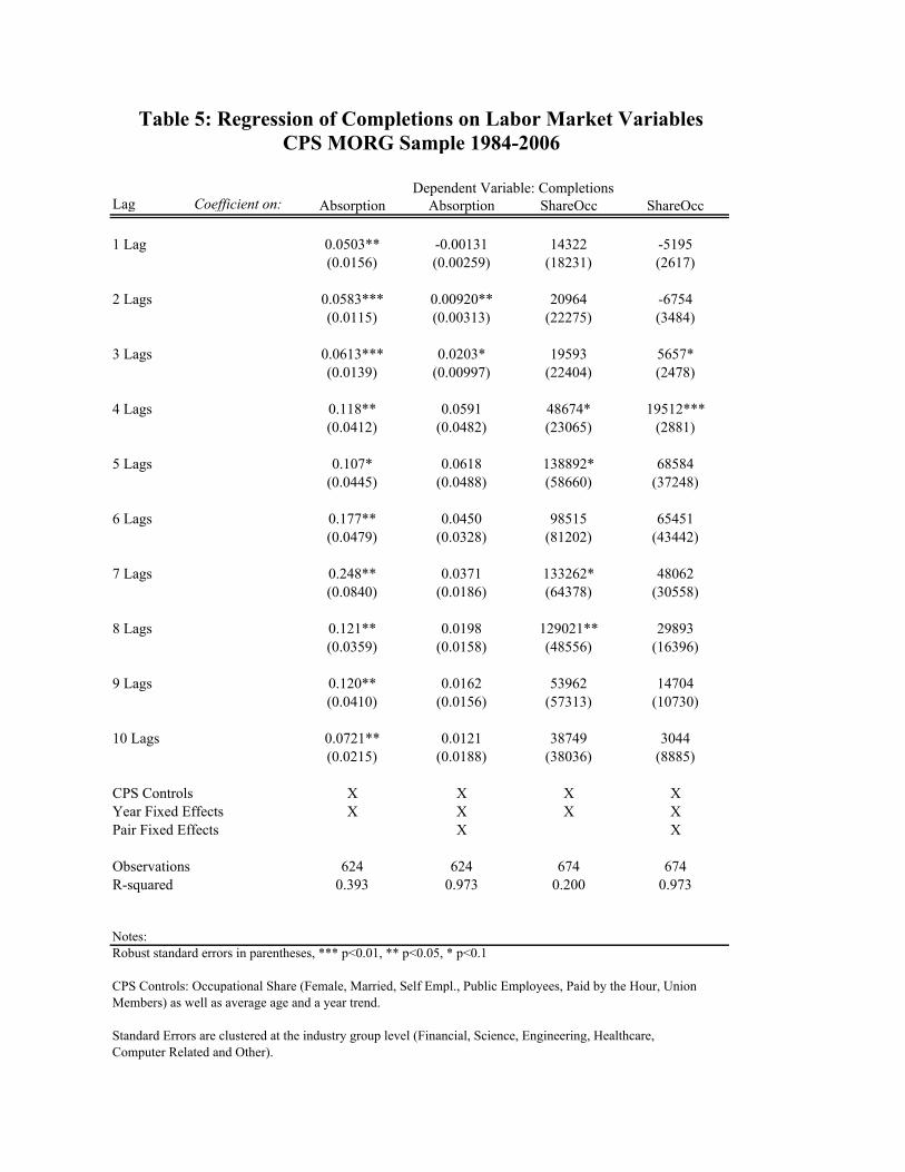
Lag Coefficient on: Absorption Absorption ShareOcc ShareOcc

1 Lag 0.0503** -0.00131 14322 -5195

(0.0156) (0.00259) (18231) (2617)

2 Lags 0.0583*** 0.00920** 20964 -6754

(0.0115) (0.00313) (22275) (3484)

3 Lags 0.0613*** 0.0203* 19593 5657*

(0.0139) (0.00997) (22404) (2478)

4 Lags 0.118** 0.0591 48674* 19512***

(0.0412) (0.0482) (23065) (2881)

5 Lags 0.107* 0.0618 138892* 68584

(0.0445) (0.0488) (58660) (37248)

6 Lags 0.177** 0.0450 98515 65451

(0.0479) (0.0328) (81202) (43442)

7 Lags 0.248** 0.0371 133262* 48062

(0.0840) (0.0186) (64378) (30558)

8 Lags 0.121** 0.0198 129021** 29893

(0.0359) (0.0158) (48556) (16396)

9 Lags 0.120** 0.0162 53962 14704

(0.0410) (0.0156) (57313) (10730)

10 Lags 0.0721** 0.0121 38749 3044

(0.0215) (0.0188) (38036) (8885)

CPS Controls X X X X

Year Fixed Effects X X X X

Pair Fixed Effects X X

Observations 624 624 674 674

R-squared 0.393 0.973 0.200 0.973

Notes:

Robust standard errors in parentheses, *** p<0.01, ** p<0.05, * p<0.1

CPS Controls: Occupational Share (Female, Married, Self Empl., Public Employees, Paid by the Hour, Union

Members) as well as average age and a year trend.

Standard Errors are clustered at the industry group level (Financial, Science, Engineering, Healthcare,

Computer Related and Other).

Table 5: Regression of Completions on Labor Market Variables

CPS MORG Sample 1984-2006

Dependent Variable: Completions

Variables: Comp Comp ln(Comp) ln(Comp) Comp Comp

Absorption 1 Lag 0.123*** 0.0181***

(0.0321) (0.00467)

Absorption 2 Lags 0.00871 0.00607

(0.0325) (0.00706)

Absorption 3 Lags -0.0450 -0.00496

(0.0648) (0.0134)

Wage Growth 1 Lag 2.983 0.276

(2.545) (0.357)

Wage Growth 2 Lags -0.827 0.285

(3.218) (0.308)

Wage Growth 3 Lags -2.138 -0.317

(2.316) (0.268)

Shareocc Chg 1 Lag 2612*** -263.2

(999.3) (684.5)

Shareocc Chg 2 Lags 1106* -52.00

(637.6) (116.3)

Shareocc Chg 3 Lags 1551** 70.80

(751.9) (224.8)

Pair Fixed Effects X X X

CPS Controls X X X X X X

Year Fixed Effects X X X X X X

Observations 391 391 518 518 518 518

R-squared 0.298 0.993 0.112 0.994 0.330 0.985

Notes:

Robust standard errors in parentheses, *** p<0.01, ** p<0.05, * p<0.1

CPS Controls: Occupational Share (Female, Married, Self Empl., Public Employees, Paid by the Hour, Union

Members) as well as average age and a year trend.

Table 6: Regression of Completions on Labor Market Variables

BLS Sample 2000-2006

Dependent Variable:

Variables: OLS OLS OLS WLS WLS WLS IV IV IV

Absorption 1 Lag 0.0953*** 0.0642*** 0.213**

(0.0227) (0.0239) (0.0758)

Absorption 4 Lags 0.250* 0.176*** 0.327*

(0.115) (0.0591) (0.129)

Absorption 7 Lags 0.344* 0.255*** 0.624*

(0.153) (0.0534) (0.256)

CPS Controls X X X X X X X X X

Year Fixed Effects X X X X X X X X X

Clustered S.E. X X X X X X X X X

Observations 1085 936 789 1085 936 789 679 679 679

R-squared 0.096 0.148 0.179 0.087 0.117 0.144 0.058 0.137 0.109

Notes:

Robust standard errors in parentheses, *** p<0.01, ** p<0.05, * p<0.1

CPS Controls: Occupational Share (Female, Married, Self Empl., Public Employees, Paid by the Hour, Union Members) as well as average age and a year trend.

Standard errors are clustered at the industry group level (Financial, Science, Engineering, Healthcare, Computer Related and Other).

Table 7: Alternative Specifications, WLS and IV

CPS MORG Sample 1984-2006

Dependent Variable: Completions

Variable (1) (2) (3)

Ln(Real Wage) 1 Lag 0.239 0.454*** 0.426**

(0.537) (0.100) (0.123)

Ln(Real Wage) 2 Lags -0.343 0.314** 0.253

(0.552) (0.119) (0.142)

Ln(Real Wage) 3 Lags 0.824** 0.217* 0.0547

(0.310) (0.107) (0.0662)

Ln(Real Wage) 4 Lags 0.616* 0.151 0.111

(0.255) (0.126) (0.181)

Ln(Real Wage) 5 Lags 0.666*** 0.0885 0.0274

(0.118) (0.120) (0.161)

Ln(Real Wage) 6 Lags 0.155

(0.148)

Ln(Real Wage) 7 Lags 0.0104

(0.0452)

Ln(Real Wage) 8 Lags 0.0831

(0.0676)

CPS Controls X X X

Year Fixed Effects X X X

Pair Fixed Effects X X

Observations 935 935 788

R-squared 0.241 0.958 0.967

Notes:

Robust standard errors in parentheses, *** p<0.01, ** p<0.05, * p<0.1

CPS Controls: Occupational Share (Female, Married, Self Empl., Public Employees, Paid by the Hour,

Union Members) as well as average age and a year trend.

Standard errors are clustered at the industry group level (Financial, Science, Engineering, Healthcare,

Computer Related and Other).

Table 8: Regression of Log Completions on Log WagesCPS MORG Sample 1984-2006

Variable (1) (2) (3) (4)

ShareOcc_Chg 1 Lag 1.586* 0.928 0.232* 0.312**

(0.690) (0.847) (0.108) (0.0879)

ShareOcc_Chg 2 Lags 1.813 1.211 0.216 0.240*

(0.927) (0.908) (0.163) (0.101)

ShareOcc_Chg 3 Lags 1.829* 0.956 0.230 0.206

(0.897) (0.670) (0.129) (0.126)

ShareOcc_Chg 4 Lags 1.738* 0.852 0.253* 0.257**

(0.828) (0.758) (0.102) (0.0905)

ShareOcc_Chg 5 Lags 3.969*** 0.916**

(0.763) (0.269)

ShareOcc_Chg 6 Lags 5.124** 0.953***

(1.383) (0.234)

ShareOcc_Chg 7 Lags 4.395** 0.936***

(1.349) (0.104)

ShareOcc_Chg 8 Lags 3.076** 0.475***

(1.144) (0.0651)

CPS Controls X X X X

Year Fixed Effects X X X X

Pair Fixed Effects X X

Observations 980 784 980 784

R-squared 0.225 0.257 0.955 0.967

Notes:

Robust standard errors in parentheses, *** p<0.01, ** p<0.05, * p<0.1

CPS Controls: Occupational Share (Female, Married, Self Empl., Public Employees, Paid by the Hour,

Union Members) as well as average age and a year trend.

Standard errors are clustered at the industry group level (Financial, Science, Engineering, Healthcare,

Computer Related and Other).

Dependent Variable: Ln(Completions)

Table 9: Regression of Log Completions on ShareOcc MeasureCPS MORG Sample 1984-2006

Figure 1: Education/Labor Market Linkage

LABOR MARKET

Labor demand: Occupation-specific Wage and Vacancies Signals

Student Body: Response Through No. of Applications to College; degree and field

of study corresponding to occupation

EDUCATION SECTOR

Fuzzy Response of Educational Sector Output:

Long Term Flexibilitybrought about by Surge in Apps and Funding Signals

from Pvt. And Public Sector

Sorting/matching

of

skills/capabilities

with interests

Acceptance

Ratio; Completion

Ratio

Immigration;

H1BRetirement

a) Linkages Between Labor Market and the Higher

Education Complex: Structure, Signals, Responses

D1

D2

S Responsive

S Unresponsive

Net Societal Gain

Wages

EmploymentERE0,U

WU

WR

W0

Figure 2: Welfare and Labor Supply Elasticity

Figure 3: Growth of Post-Secondary Completions

by Degree Level, 1984-2006

0.00%

2.00%

4.00%

6.00%

8.00%

10.00%

12.00%

14.00%

Award of <1

Year

Award of

>=1 but <2

Years

Associate Bachelor Masters Doctoral First

Professional

Degree

Total

Average Annual Growth Rate .

Source: Completions from IPEDS, 1999 excluded.

First Professional Degrees include specialty degrees such as M.D., D.M.D., D.V.M., and D.C..

Figure 4: Post-Secondary Degrees Conferred

by Broad Degree Program, 1984-2006

0

50,000

100,000

150,000

200,000

250,000

300,000

350,000

400,000

450,000

500,000

1985–86 1990–91 1995–96 2000–01 2005–06

Degrees

Humanities

Natural Sciences

Computer Scienceand Engineering

Business

Source: National Center for Economic Statistics, Digest of Education Statistics, Various Years

Figure 5: Annual Output of Post-Secondary Degrees, Net Change in

Employment and Wages, 1984-2006

-2,000,000

-1,000,000

0

1,000,000

2,000,000

3,000,000

4,000,000

5,000,000

1984

1985

1986

1987

1988

1989

1990

1991

1992

1993

1994

1995

1996

1997

1998

1999

2000

2001

2002

2003

2004

2005

2006

$-

$5,000

$10,000

$15,000

$20,000

$25,000

$30,000

$35,000

$40,000

$45,000

$50,000

Absorptions(Left Axis)

Completions(Left Axis)

Real Wage(Right Axis)

Source: Completions from IPEDS, 1999 linearly interpolated. Real wage and absorption data from CEPR CPS ORG

extracts. Absorptions are not smoothed.

Figure 6: Correlation of Degree Completions with Labor Market

Absorption Including Lags across all Paired Occupations

0

0.05

0.1

0.15

0.2

0.25

0.3

0.35

0 1 2 3 4 5 6 7 8 9 10

Absorption Lag (Years)

Unweighted

Employment Weighted

Figure 7: Computer ScientistsDegree Completions, Employment Changes, and Wages, 1984-2006

-100,000

-50,000

0

50,000

100,000

150,000

200,000

250,000

1984

1985

1986

1987

1988

1989

1990

1991

1992

1993

1994

1995

1996

1997

1998

1999

2000

2001

2002

2003

2004

2005

2006

$-

$10,000

$20,000

$30,000

$40,000

$50,000

$60,000

$70,000

$80,000

Absorptions(Left Axis)

Completions(Left Axis)

Real Wage(Right Axis)

Source: Completions from IPEDS, 1999 linearly interpolated. Real wage and absorption data from CEPR CPS ORG

extracts. Absorptions are a smoothed using a 3 year moving average.

Figure 8: ArchitectsDegree Completions, Employment Changes, and Wages, 1984-2006

-15,000

-10,000

-5,000

0

5,000

10,000

15,000

20,000

25,000

1984

1985

1986

1987

1988

1989

1990

1991

1992

1993

1994

1995

1996

1997

1998

1999

2000

2001

2002

2003

2004

2005

2006

$-

$10,000

$20,000

$30,000

$40,000

$50,000

$60,000

$70,000

$80,000

Absorptions(Left Axis)

Completions(Left Axis)

Real Wage(Right Axis)

Source: Completions from IPEDS, 1999 linearly interpolated. Real wage and absorption data from CEPR CPS ORG extracts.

Absorptions are a smoothed using a 3 year moving average.

Figure 9: PhysiciansDegree Completions, Employment Changes, and Wages, 1984-2002

-10,000

-5,000

0

5,000

10,000

15,000

20,000

25,000

30,000

35,000

40,000

1984

1985

1986

1987

1988

1989

1990

1991

1992

1993

1994

1995

1996

1997

1998

1999

2000

2001

2002

$-

$20,000

$40,000

$60,000

$80,000

$100,000

$120,000

$140,000

Absorptions(Left Axis)

Completions(Left Axis)

Real Wage(Right Axis)

Source: Completions from IPEDS, 1999 linearly interpolated. Real wage and absorption data from CEPR CPS ORG extracts.

Absorptions are a smoothed using a 3 year moving average.

Figure 10: Licensed Practical NurseDegree Completions, Employment Changes, and Wages, 1984-2006

-40,000

-30,000

-20,000

-10,000

0

10,000

20,000

30,000

40,000

50,000

60,000

1984

1985

1986

1987

1988

1989

1990

1991

1992

1993

1994

1995

1996

1997

1998

1999

2000

2001

2002

2003

2004

2005

2006

$-

$5,000

$10,000

$15,000

$20,000

$25,000

$30,000

$35,000

$40,000

Absorptions(Left Axis)

Completions(Left Axis)

Real Wage(Right Axis)

Source: Completions from IPEDS, 1999 linearly interpolated. Real wage and absorption data from CEPR CPS ORG extracts.

Absorptions are a smoothed using a 3 year moving average.