How to get bounds for distribution convolutions?

A simulation study and an application to risk management

V. Durrleman, A. Nikeghbali & T. Roncalli∗

Groupe de Recherche OperationnelleCredit Lyonnais

France

September 10, 2000

Abstract

In this paper, we consider the problem of bounds for distribution convolutions and we present someapplications to risk management. We show that the upper Frechet bound is not always the more riskydependence structure. It is in contradiction with the belief in finance that maximal risk correspond to thecase where the random variables are comonotonic.

1 Introduction

We consider here two problems applied to finance. The first one is the Kolmogorov problem and we show howMakarov inequalities could be used in risk management. The second one is based on the Kantorovich distancebetween two distributions. For this two problem, we show that maximal risk does not correspond to the casewhere the random variables are comonotonic.

2 Distribution convolutions and Makarov inequalities

In this section, we apply the Makarov inequalities to risk aggregation.

2.1 The triangle functions and σ−operations

We note ∆+ the space of probability distribution functions whose support is contained in R+. Schweizer[1991] gives the following definition for a triangle function:

Definition 1 Given a function τ : ∆+ ×∆+ −→ ∆+, τ is a triangle function if it satisfies1

1. τ (F, ε0) = F;

2. τ (F1,F2) = τ (F2,F1);

3. τ (F1,F2) ≤ τ (G1,G2) whenever F1 (x) ≤ G1 (x) and F2 (x) ≤ G2 (x) for x ∈ R+;

∗Corresponding author: Groupe de Recherche Operationnelle, Bercy-Expo — Immeuble Bercy Sud — 4e etage, 90 quai de Bercy— 75613 Paris Cedex 12 — France; E-mail adress: thierry.roncalli@creditlyonnais.fr

1ε0 is the unit step-function

ε0 (x) =

�0 if x ≤ 01 if x > 0

(1)

1

4. τ (τ (F1,F2) ,F3) = τ (F1, τ (F2,F3));

Schweizer and Sklar [1983] define also a probabilistic metric space as the ordered triple (S,z,τ) whereS is a set, z is a mapping from S × S into ∆+ and τ a triangle function. Schweizer [1991] does the followinginterpretation:

In short, probabilistic metric spaces are generalizations of ordinary metric spaces in which R+ isreplaced by the set ∆+ and the operation of addition on R+ is replaced by a triangle function.

Two triangle functions play a special role. Let B be the class of Borel-measurable two place functions. LetX1 and X2 be two random variables with distributions F1 and F2. We then consider the random variableX = L (X1, X2) with distribution G and L ∈ B. The supremal convolution τC,L (F1,F2) is

τC,L (F1,F2) (x) = supL(x1,x2)=x

C (F1 (x1) ,F2 (x2)) (2)

whereas the infimal convolution ρC,L (F1,F2) corresponds to

ρC,L (F1,F2) (x) = infL(x1,x2)=x

C (F1 (x1) ,F2 (x2)) (3)

with C the dual of the copula C. Another important function is the σ−convolution (Frank [1991]) defined by

σC,L (F1,F2) (x) =∫

L(x1,x2)<x

dC (F1 (x1) ,F2 (x2)) (4)

In general, we have

τC−,L (F1,F2) ≤ τC,L (F1,F2) ≤ σC,L (F1,F2) ≤ ρC,L (F1,F2) ≤ ρC−,L (F1,F2) (5)

2.2 The dependency bounds

Dependency bounds are related to a Kolmogorov’s problem (Makarov [1981]): find distribution function G∨and G∧ such that for all x in R, G∨ (x) = inf Pr {X1 + X2 < x} and G∧ (x) = sup Pr {X1 + X2 < x} wherethe infimum and supremum are taken over all possible joint distribution functions having margins F1 and F2.The solution is then G∨ = τC−,+ (F1,F2) and G∧ = ρC−,+ (F1,F2).

This solution has a long history (see the section eight of Schweizer [1991]). Note that it holds even for nonpositive random variables and moreover these bounds cannot be improved (Frank, Nelsen and Schweizer[1987]). Williamson [1989] extends this result when C− ≺ C and L denotes the four arithmetic operators (+,−, × and ÷).

Theorem 2 Let X1 and X2 be two positive random variables with distributions F1 and F2 and dependencestructure C such that C− ≺ C. Then, the distribution G of X = L (X1, X2) is contained within the boundsG∨ (x)≤ G (x)≤ G∧ (x) with G∨ (x) = τC−,L (F1,F2) (x) and G∧ (x) = ρC−,L (F1,F2) (x). These boundsare the pointwise best possible.

Williamson and Downs [1990] remark that knowing a tighter lower bound than the lower Frechet bound(C− ≺ C− ≺ C) provide tighter bounds G∨ and G∧, but knowing a tighter upper bound than the upperFrechet bound (C ≺ C+ ≺ C+) has curiously no effect on the dependency bounds!

2

2.3 Duality of infimal and supremal convolutions

Let F be a distribution. We note F(−1) the inverse of F, that is F(−1) (u) = sup {x | F (x) < u}. Frank andSchweizer [1979] show then that τC,L (F1,F2) = τ

(−1)C,L

(F(−1)

1 ,F(−1)2

)and ρC,L (F1,F2) = ρ

(−1)C,L

(F(−1)

1 ,F(−1)2

)

withτC,L

(F(−1)

1 ,F(−1)2

)(u) = inf

C(u1,u2)=uL

(F(−1)

1 (u1) ,F(−1)2 (u2)

)(6)

andρC,L

(F(−1)

1 ,F(−1)2

)(u) = sup

C(u1,u2)=u

L(F(−1)

1 (u1) ,F(−1)2 (u2)

)(7)

Williamson and Downs [1990] derive then numerical algorithms to compute the dependency bounds G∨ andG∧. For example, if C− = C− and L is the operation +, we have

G(−1)∨ (u) = inf

max(u1+u2−1,0)=uF(−1)

1 (u1) + F(−1)2 (u2)

= infv∈[u,1]

F(−1)1 (v) + F(−1)

2 (u− v + 1) (8)

and

G(−1)∧ (u) = sup

min(u1+u2,1)=u

F(−1)1 (u1) + F(−1)

2 (u2)

= supv∈[0,u]

F(−1)1 (v) + F(−1)

2 (u− v) (9)

2.4 Some simulations

Frank, Nelsen and Schweizer [1987] derive analytical expressions of the dependency bounds in the case ofgaussian, Cauchy and exponential distributions when C− = C− and L is the operation +. We present nowsome simulations based on the numerical algorithms of Williamson and Downs [1990].

We consider the example when X1 and X2 are two gaussian distributions N (µ1, σ1) and N (µ2, σ2). If thedependence structure is Normal with parameter ρ, it comes that the distribution G of X1 + X2 is gaussianand we have G = N

(µ1 + µ2,

√σ2

1 + 2ρσ1σ2 + σ22

). The lower and upper dependency bounds are given by

equations (8) and (9) when C− = C−. If C− = C⊥, G∨ and G∧ becomes

G(−1)∨ (u) = inf

v∈[0,1]F(−1)

1 (v) + F(−1)2

(u

v

)(10)

and

G(−1)∧ (u) = sup

v∈[0,1]

F(−1)1 (v) + F(−1)

2

(u− v

1− v

)(11)

In the case where C− = C+, we obtain the following results

G(−1)∨ (u) = inf

min(u1,u2)=uF(−1)

1 (u1) + F(−1)2 (u2)

= supmax(u1,u2)=u

F(−1)1 (u1) + F(−1)

2 (u2)

= supu1+u2−min(u1,u2)=u

F(−1)1 (u1) + F(−1)

2 (u2)

= G(−1)∧ (u) (12)

We have reported in the figure 1 the dependency bounds when µ1 = 1, µ2 = 2, σ1 = 2 and σ2 = 1 in the caseC− = C−. Moreover, we have represented the distribution G when the dependence structure is respectively

3

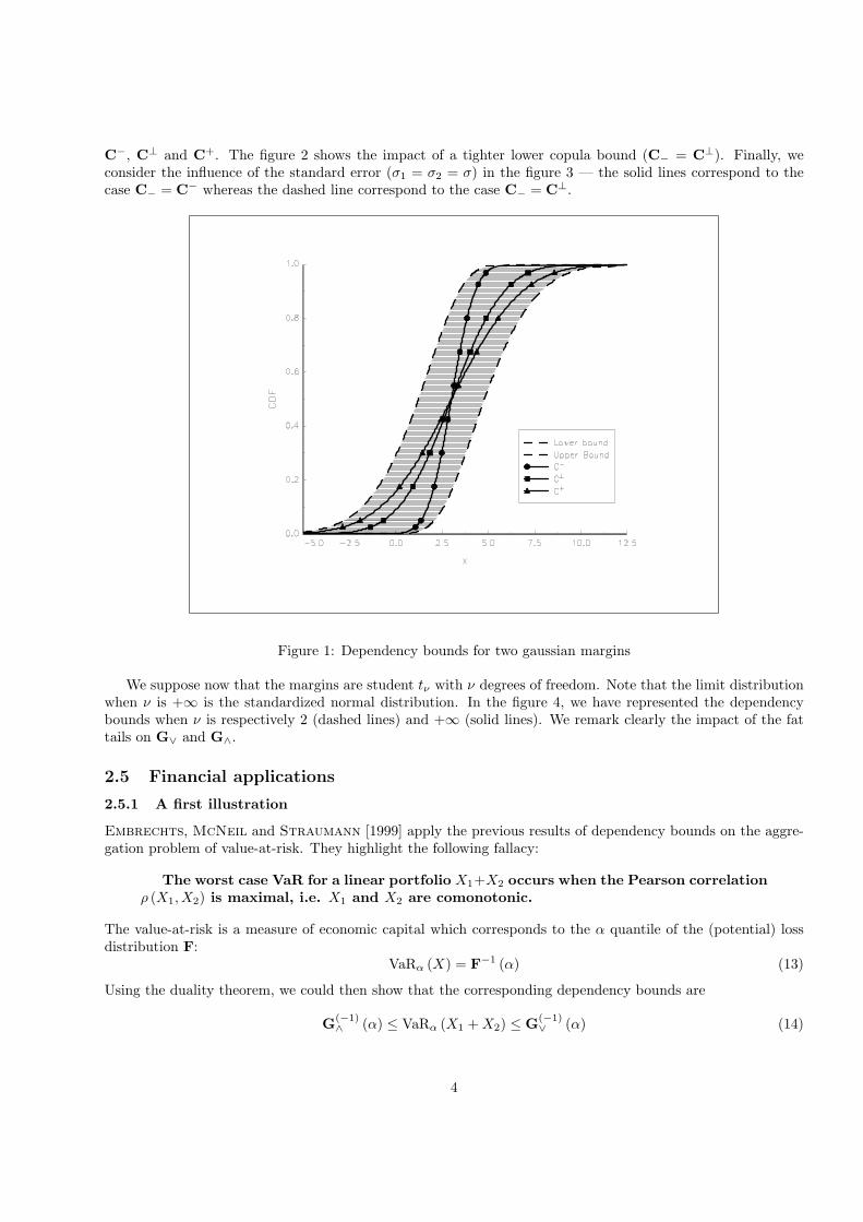
C−, C⊥ and C+. The figure 2 shows the impact of a tighter lower copula bound (C− = C⊥). Finally, weconsider the influence of the standard error (σ1 = σ2 = σ) in the figure 3 — the solid lines correspond to thecase C− = C− whereas the dashed line correspond to the case C− = C⊥.

Figure 1: Dependency bounds for two gaussian margins

We suppose now that the margins are student tν with ν degrees of freedom. Note that the limit distributionwhen ν is +∞ is the standardized normal distribution. In the figure 4, we have represented the dependencybounds when ν is respectively 2 (dashed lines) and +∞ (solid lines). We remark clearly the impact of the fattails on G∨ and G∧.

2.5 Financial applications

2.5.1 A first illustration

Embrechts, McNeil and Straumann [1999] apply the previous results of dependency bounds on the aggre-gation problem of value-at-risk. They highlight the following fallacy:

The worst case VaR for a linear portfolio X1+X2 occurs when the Pearson correlationρ (X1, X2) is maximal, i.e. X1 and X2 are comonotonic.

The value-at-risk is a measure of economic capital which corresponds to the α quantile of the (potential) lossdistribution F:

VaRα (X) = F−1 (α) (13)

Using the duality theorem, we could then show that the corresponding dependency bounds are

G(−1)∧ (α) ≤ VaRα (X1 + X2) ≤ G(−1)

∨ (α) (14)

4

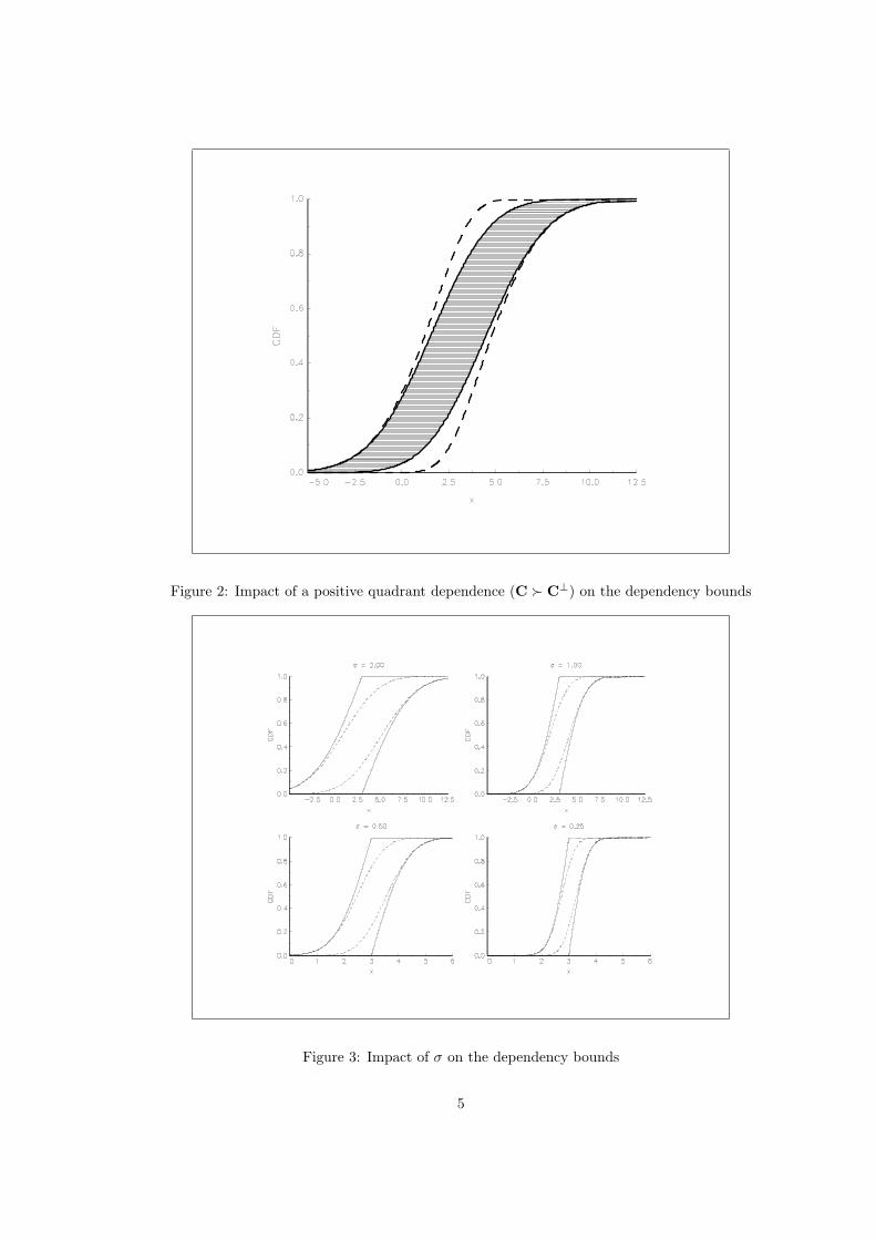
Figure 2: Impact of a positive quadrant dependence (C Â C⊥) on the dependency bounds

Figure 3: Impact of σ on the dependency bounds

5

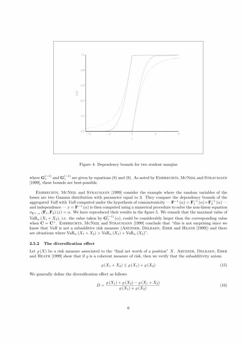
Figure 4: Dependency bounds for two student margins

where G(−1)∧ and G(−1)

∨ are given by equations (8) and (9). As noted by Embrechts, McNeil and Straumann[1999], these bounds are best-possible.

Embrechts, McNeil and Straumann [1999] consider the example where the random variables of thelosses are two Gamma distribution with parameter equal to 3. They compare the dependency bounds of theaggregated VaR with VaR computed under the hypothesis of comonotonicity — F−1 (α) = F−1

1 (α)+F−12 (α) —

and independence — x = F−1 (α) is then computed using a numerical procedure to solve the non-linear equationσC⊥,+ (F1,F2) (x) = α. We have reproduced their results in the figure 5. We remark that the maximal value ofVaRα (X1 + X2), i.e. the value taken by G(−1)

∨ (α), could be considerably larger than the corresponding valuewhen C = C+. Embrechts, McNeil and Straumann [1999] conclude that “this is not surprising since weknow that VaR is not a subadditive risk measure (Artzner, Delbaen, Eber and Heath [1999]) and thereare situations where VaRα (X1 + X2) > VaRα (X1) + VaRα (X2)”.

2.5.2 The diversification effect

Let % (X) be a risk measure associated to the “final net worth of a position” X. Artzner, Delbaen, Eberand Heath [1999] show that if % is a coherent measure of risk, then we verify that the subadditivity axiom

% (X1 + X2) ≤ % (X1) + % (X2) (15)

We generally define the diversification effect as follows

D =% (X1) + % (X2)− % (X1 + X2)

% (X1) + % (X2)(16)

6

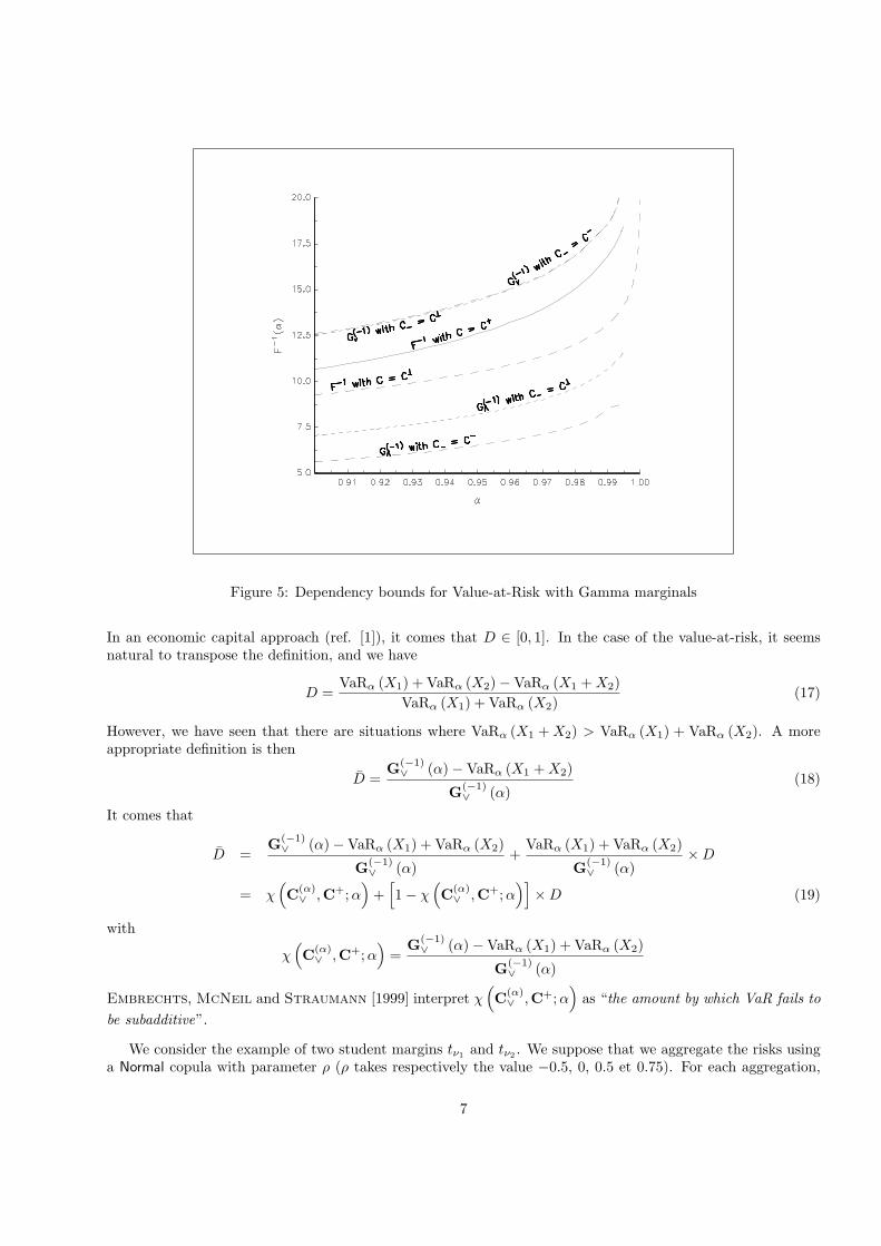
Figure 5: Dependency bounds for Value-at-Risk with Gamma marginals

In an economic capital approach (ref. [1]), it comes that D ∈ [0, 1]. In the case of the value-at-risk, it seemsnatural to transpose the definition, and we have

D =VaRα (X1) + VaRα (X2)−VaRα (X1 + X2)

VaRα (X1) + VaRα (X2)(17)

However, we have seen that there are situations where VaRα (X1 + X2) > VaRα (X1) + VaRα (X2). A moreappropriate definition is then

D =G(−1)∨ (α)−VaRα (X1 + X2)

G(−1)∨ (α)

(18)

It comes that

D =G(−1)∨ (α)−VaRα (X1) + VaRα (X2)

G(−1)∨ (α)

+VaRα (X1) + VaRα (X2)

G(−1)∨ (α)

×D

= χ(C(α)∨ ,C+;α

)+

[1− χ

(C(α)∨ ,C+; α

)]×D (19)

with

χ(C(α)∨ ,C+;α

)=

G(−1)∨ (α)−VaRα (X1) + VaRα (X2)

G(−1)∨ (α)

Embrechts, McNeil and Straumann [1999] interpret χ(C(α)∨ ,C+; α

)as “the amount by which VaR fails to

be subadditive”.

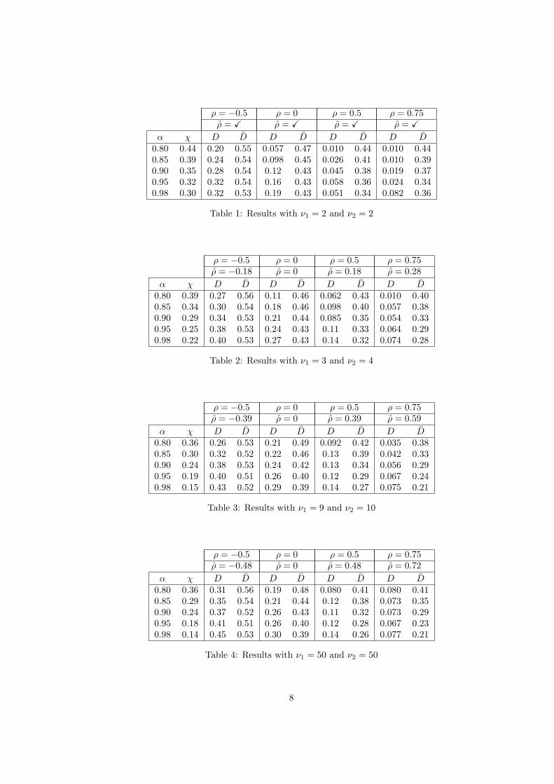
We consider the example of two student margins tν1 and tν2 . We suppose that we aggregate the risks usinga Normal copula with parameter ρ (ρ takes respectively the value −0.5, 0, 0.5 et 0.75). For each aggregation,

7

ρ = −0.5 ρ = 0 ρ = 0.5 ρ = 0.75ρ = X ρ = X ρ = X ρ = X

α χ D D D D D D D D0.80 0.44 0.20 0.55 0.057 0.47 0.010 0.44 0.010 0.440.85 0.39 0.24 0.54 0.098 0.45 0.026 0.41 0.010 0.390.90 0.35 0.28 0.54 0.12 0.43 0.045 0.38 0.019 0.370.95 0.32 0.32 0.54 0.16 0.43 0.058 0.36 0.024 0.340.98 0.30 0.32 0.53 0.19 0.43 0.051 0.34 0.082 0.36

Table 1: Results with ν1 = 2 and ν2 = 2

ρ = −0.5 ρ = 0 ρ = 0.5 ρ = 0.75ρ = −0.18 ρ = 0 ρ = 0.18 ρ = 0.28

α χ D D D D D D D D0.80 0.39 0.27 0.56 0.11 0.46 0.062 0.43 0.010 0.400.85 0.34 0.30 0.54 0.18 0.46 0.098 0.40 0.057 0.380.90 0.29 0.34 0.53 0.21 0.44 0.085 0.35 0.054 0.330.95 0.25 0.38 0.53 0.24 0.43 0.11 0.33 0.064 0.290.98 0.22 0.40 0.53 0.27 0.43 0.14 0.32 0.074 0.28

Table 2: Results with ν1 = 3 and ν2 = 4

ρ = −0.5 ρ = 0 ρ = 0.5 ρ = 0.75ρ = −0.39 ρ = 0 ρ = 0.39 ρ = 0.59

α χ D D D D D D D D0.80 0.36 0.26 0.53 0.21 0.49 0.092 0.42 0.035 0.380.85 0.30 0.32 0.52 0.22 0.46 0.13 0.39 0.042 0.330.90 0.24 0.38 0.53 0.24 0.42 0.13 0.34 0.056 0.290.95 0.19 0.40 0.51 0.26 0.40 0.12 0.29 0.067 0.240.98 0.15 0.43 0.52 0.29 0.39 0.14 0.27 0.075 0.21

Table 3: Results with ν1 = 9 and ν2 = 10

ρ = −0.5 ρ = 0 ρ = 0.5 ρ = 0.75ρ = −0.48 ρ = 0 ρ = 0.48 ρ = 0.72

α χ D D D D D D D D0.80 0.36 0.31 0.56 0.19 0.48 0.080 0.41 0.080 0.410.85 0.29 0.35 0.54 0.21 0.44 0.12 0.38 0.073 0.350.90 0.24 0.37 0.52 0.26 0.43 0.11 0.32 0.073 0.290.95 0.18 0.41 0.51 0.26 0.40 0.12 0.28 0.067 0.230.98 0.14 0.45 0.53 0.30 0.39 0.14 0.26 0.077 0.21

Table 4: Results with ν1 = 50 and ν2 = 50

8

we compute D, D and χ(C(α)∨ ,C+; α

)for different confidence levels. The results are given in the tables 1–

4. Moreover, we have reported also the Pearson correlation ρ. With this example, we could do the followingremarks:

1. the diversification effect does not depend only on the correlation, but also on marginal distributions;

2. the dependence structure (i.e. the copula used to perform the aggregation) plays a more important rolethan the correlation for determining the diversification effect;

3. a lower correlation does not imply systematically a greater diversification effect.

2.5.3 The ‘square root’ rule

In the finance industry, the aggregation is often done using the ‘square root’ rule

VaRα (X1 + X2) =√

[VaRα (X1)]2 + 2ρ (X1, X2)VaRα (X1)VaRα (X2) + [VaRα (X2)]

2 (20)

with ρ (X1, X2) the Pearson correlation between the two random variables X1 + X2. When ρ (X1, X2) = 1, weobtain of course VaRα (X1 + X2) = VaRα (X1) + VaRα (X2). Sometimes, risk managers have no ideas aboutthe value of ρ (X1, X2) and suppose ρ (X1, X2) = 0. This could be justified in operational risk measurement.For market risk measurement, the justification is more difficult in the case of the risk aggregation by desks.However, this rule is sometimes used when the aggregation is performed by markets (for example, bond, equityand commodities markets) because of the segmentation assumption.

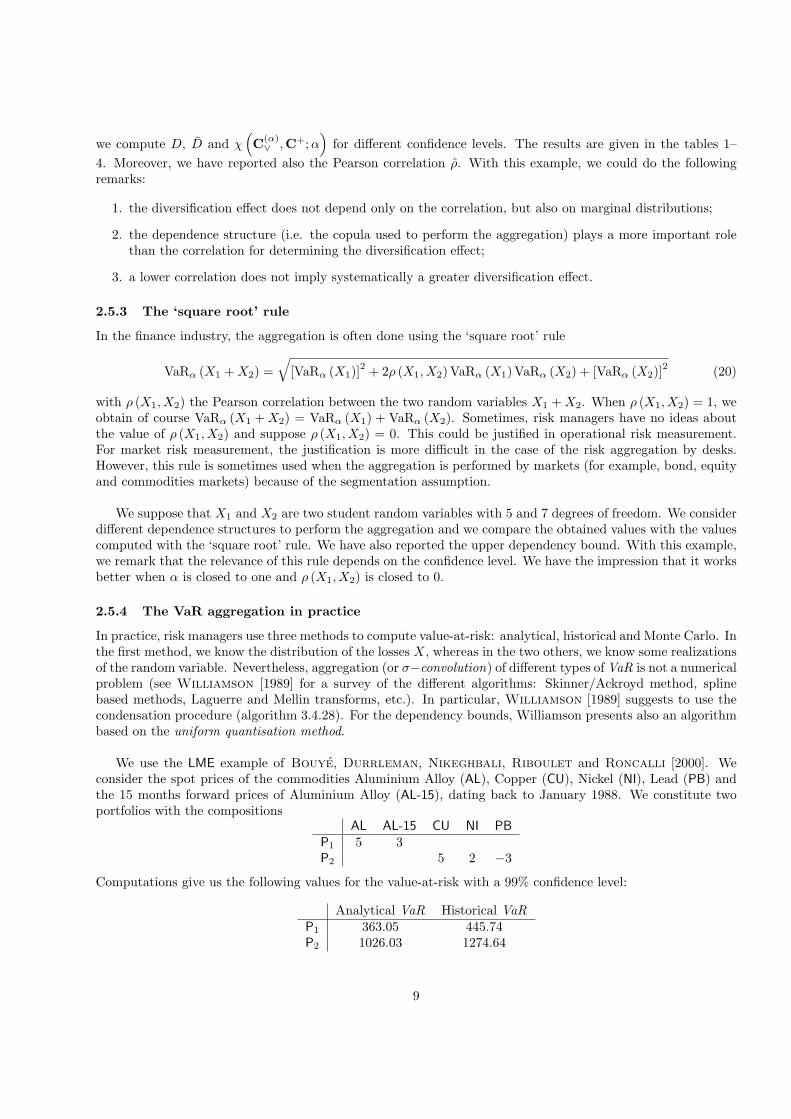
We suppose that X1 and X2 are two student random variables with 5 and 7 degrees of freedom. We considerdifferent dependence structures to perform the aggregation and we compare the obtained values with the valuescomputed with the ‘square root’ rule. We have also reported the upper dependency bound. With this example,we remark that the relevance of this rule depends on the confidence level. We have the impression that it worksbetter when α is closed to one and ρ (X1, X2) is closed to 0.

2.5.4 The VaR aggregation in practice

In practice, risk managers use three methods to compute value-at-risk: analytical, historical and Monte Carlo. Inthe first method, we know the distribution of the losses X, whereas in the two others, we know some realizationsof the random variable. Nevertheless, aggregation (or σ−convolution) of different types of VaR is not a numericalproblem (see Williamson [1989] for a survey of the different algorithms: Skinner/Ackroyd method, splinebased methods, Laguerre and Mellin transforms, etc.). In particular, Williamson [1989] suggests to use thecondensation procedure (algorithm 3.4.28). For the dependency bounds, Williamson presents also an algorithmbased on the uniform quantisation method.

We use the LME example of Bouye, Durrleman, Nikeghbali, Riboulet and Roncalli [2000]. Weconsider the spot prices of the commodities Aluminium Alloy (AL), Copper (CU), Nickel (NI), Lead (PB) andthe 15 months forward prices of Aluminium Alloy (AL-15), dating back to January 1988. We constitute twoportfolios with the compositions

AL AL-15 CU NI PBP1 5 3P2 5 2 −3

Computations give us the following values for the value-at-risk with a 99% confidence level:

Analytical VaR Historical VaRP1 363.05 445.74P2 1026.03 1274.64

9

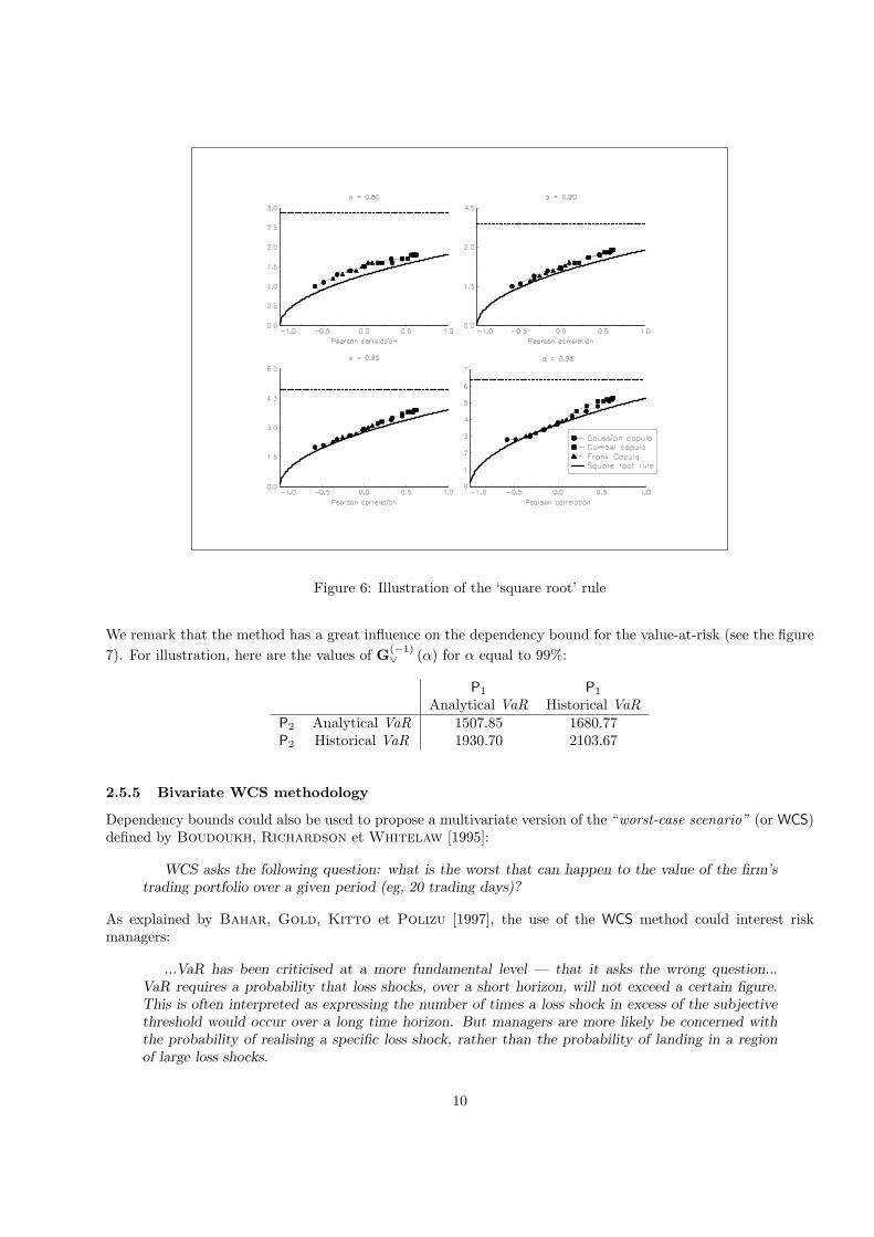
Figure 6: Illustration of the ‘square root’ rule

We remark that the method has a great influence on the dependency bound for the value-at-risk (see the figure7). For illustration, here are the values of G(−1)

∨ (α) for α equal to 99%:

P1 P1

Analytical VaR Historical VaRP2 Analytical VaR 1507.85 1680.77P2 Historical VaR 1930.70 2103.67

2.5.5 Bivariate WCS methodology

Dependency bounds could also be used to propose a multivariate version of the “worst-case scenario” (or WCS)defined by Boudoukh, Richardson et Whitelaw [1995]:

WCS asks the following question: what is the worst that can happen to the value of the firm’strading portfolio over a given period (eg, 20 trading days)?

As explained by Bahar, Gold, Kitto et Polizu [1997], the use of the WCS method could interest riskmanagers:

...VaR has been criticised at a more fundamental level — that it asks the wrong question...VaR requires a probability that loss shocks, over a short horizon, will not exceed a certain figure.This is often interpreted as expressing the number of times a loss shock in excess of the subjectivethreshold would occur over a long time horizon. But managers are more likely be concerned withthe probability of realising a specific loss shock, rather than the probability of landing in a regionof large loss shocks.

10

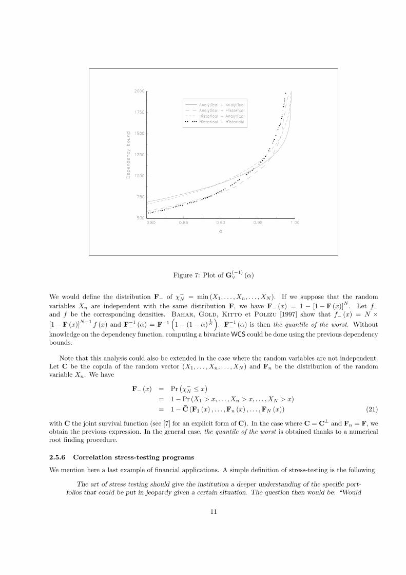
Figure 7: Plot of G(−1)∨ (α)

We would define the distribution F− of χ−N = min (X1, . . . , Xn, . . . , XN ). If we suppose that the randomvariables Xn are independent with the same distribution F, we have F− (x) = 1 − [1− F (x)]N . Let f−and f be the corresponding densities. Bahar, Gold, Kitto et Polizu [1997] show that f− (x) = N ×[1− F (x)]N−1

f (x) and F−1− (α) = F−1

(1− (1− α)

1N

). F−1

− (α) is then the quantile of the worst. Withoutknowledge on the dependency function, computing a bivariate WCS could be done using the previous dependencybounds.

Note that this analysis could also be extended in the case where the random variables are not independent.Let C be the copula of the random vector (X1, . . . , Xn, . . . , XN ) and Fn be the distribution of the randomvariable Xn. We have

F− (x) = Pr(χ−N ≤ x

)

= 1− Pr (X1 > x, . . . ,Xn > x, . . . ,XN > x)= 1− C (F1 (x) , . . . ,Fn (x) , . . . ,FN (x)) (21)

with C the joint survival function (see [7] for an explicit form of C). In the case where C = C⊥ and Fn = F, weobtain the previous expression. In the general case, the quantile of the worst is obtained thanks to a numericalroot finding procedure.

2.5.6 Correlation stress-testing programs

We mention here a last example of financial applications. A simple definition of stress-testing is the following

The art of stress testing should give the institution a deeper understanding of the specific port-folios that could be put in jeopardy given a certain situation. The question then would be: “Would

11

this be enough to bring down the firm?” That way, each institution can know exactly what scenarioit is they do not want to engage in (Michael Ong, ABN Amro, in Dunbar and Irving [1998]).

In a quantitative stress-testing program, one of the big difficulty is to stress the correlation and to measure itsimpact. The effect of the worst situation could then be computed with the dependency bounds.

3 The Kantorovich distance based method

3.1 The Dall’aglio problem

Barrio, Gine and Matran [1999] define the Kantorovich distance or L1-Wasserstein distance between twoprobability measures P1 and P2 as

d1 (P1,P2) := inf{∫∫

R2|x1 − x2| dµ (x1, x2) : µ ∈ P (

R2)

with marginals F1 and F2

}(22)

We can write it in another way:d1 (P1,P2) = inf

F∈F(F1,F2)E |X1 −X2| (23)

where F is taken on the set of all probability with marginals F1 and F2 — F belongs to the Frechet classF (F1,F2).Shorack and Wellner [1986] showed that if F1 and F2 are the distribution functions associated to P1 andP2, then we have

d1 (P1,P2) =∫ +∞

−∞|F2 (x)− F1 (x)| dx (24)

or

d1 (P1,P2) =∫ 1

0

∣∣F−12 (x)− F−1

1 (x)∣∣ dx (25)

We can remark that when P1 is equal to P2, the Frechet upper bound copula C+ is the solution of the problem.More generally, Dall’aglio [1991] showed that there is a set of minimizing joint distribution functions:

• the largest is F+ (x1, x2) = C+ (F1 (x1) ,F2 (x2));

• the smallest is

F− (x1, x2) = 1[x1≤x2]

[F1 (x1)−

(inf

x1≤x≤x2[F1 (x)− F2 (x)]

)+]

+

1[x1>x2]

[F2 (x2)−

(inf

x2≤x≤x1[F2 (x)− F1 (x)]

)+]

(26)

• any convex combination of F+ and F− is still a solution of (23).

3.2 Financial applications

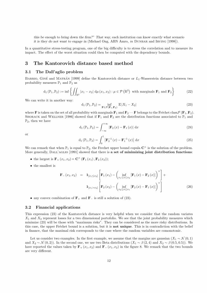
This expression (23) of the Kantorovich distance is very helpful when we consider that the random variatesX1 and X2 represent losses for a two dimensional portofolio. We see that the joint probability measures whichminimize (23) will be those with “maximum risks”. They can be considered as the more risky distributions. Inthis case, the upper Frechet bound is a solution, but it is not unique. This is in contradiction with the beliefin finance, that the maximal risk corresponds to the case where the random variables are comonotonic.

Let us consider two examples. In the first example, we assume that the margins are gaussian (X1 ∼ N (0, 1)and X2 ∼ N (0, 2)). In the second one, we use two Beta distributions (X1 ∼ β (2, 4) and X2 ∼ β (0.5, 0.5)). Wehave reported the values taken by F+ (x1, x2) and F− (x1, x2) in the figure 8. We remark that the two boundsare very different.

12

Figure 8: Illustration of the Dall’aglio problem

4 Conclusion

In this paper, we apply the dependency bounds to the value-at-risk problem, and show that the more riskydistribution is not always the upper Frechet copula.

References

[1] Amendment to the capital accord to incorporate market risks, Basle Committee on Banking Supervision,January 1996, N◦ 24

[2] Artzner, A., F. Delbaen, J-M. Eber and D. Heath [1999], Coherent measures of risk, MathematicalFinance, 9, 203-228

[3] Bahar, R., M. Gold, T. Kitto and C. Polizu [1997], Making the best of the worst, Risk Magazine, 10,August

[4] Barrio E. (del), E. Gine and C. Matran [1999], Central limit theorems for the Wasserstein distancebetween the empirical and the true distributions, Annals of Probability, 27, 1009-1071

[5] Barrio E. (del), J.A. Cuesta Albertos, C. Matran and J. Rodrıguez Rodrıguez [1999], Tests ofgoodness of fit based on the L2-Wasserstein distance, Annals of Statistics, 27, 1230-1239

[6] Boudoukh, J., M. Richardson et R. Whitelaw [1995], Expect the worst, Risk Magazine, 8, September

[7] Bouye, E., V. Durrleman, A. Nikeghbali, G. Riboulet and T. Roncalli [2000], Copulas for finance— A reading guide and some applications, Groupe de Recherche Operationnelle, Credit Lyonnais, WorkingPaper

13

[8] Dall’Aglio, G. [1991], Frechet classes: the beginnings, in G. Dall’Aglio, S. Kotz and G. Salinetti (Eds.),Advances in Probability Distributions with Given Marginals (Beyond the Copulas), Kluwer Academic Pub-lishers, Dordrecht

[9] Dall’Aglio, G., S. Kotz and G. Salinetti [1991], Advances in Probability Distributions with GivenMarginals (Beyond the Copulas), Kluwer Academic Publishers, Dordrecht

[10] Dunbar, N. and R. Irving [1998], This is the way the world ends, Risk Magazine, 11, December

[11] Embrechts, P., McNeil, A.J. and D. Straumann [1999], Correlation and dependency in risk manage-ment: properties and pitfalls, Departement of Mathematik, ETHZ, Zurich, Working Paper

[12] Frank, M.J. [1991], Convolutions for dependent random variables, in G. Dall’Aglio, S. Kotz and G.Salinetti (Eds.), Advances in Probability Distributions with Given Marginals (Beyond the Copulas), KluwerAcademic Publishers, Dordrecht

[13] Frank, M.J., R.B. Nelsen, and B. Schweizer [1987], Best-possible bounds for the distribution of a sum— a problem of Kolmogorov, Probability Theory and Related Fields, 74, 199-211

[14] Frank, M.J. and B. Schweizer [1979], On the duality of generalized infimal and supremal convolutions,Rendiconti di Matematica, 12, 1-23

[15] Hillali, Y. [1998], Analyse et Modelisation des Donnees Probabilistes : Capacites et Lois Multidimen-sionnelles, PhD Thesis, University of Paris IX-Dauphine

[16] Li, H., M. Scarsini and M. Shaked [1996], Bounds for the distribution of a multivariate sum, in L.Rushendorf, B. Schweizer and M.D. Taylor (Eds.), Distributions with Fixed Marginals and Related Topics,Institute of Mathematical Statistics, Hayward, CA

[17] Makarov, G. [1981], Estimates for the distribution function of a sum of two random variables when themarginal distributions are fixed, Theory of Probability and its Applications, 26, 803-806

[18] Nelsen, R.B. [1998], An Introduction to Copulas, Lectures Notes in Statistics, 139, Springer Verlag, NewYork

[19] Nelsen, R.B. and B. Schweizer [1991], Bounds for distribution functions of sums of squares and radialerrors, International Journal of Mathematics and Mathematical Sciences, 14, 561-570

[20] Rushendorf, L., B. Schweizer and M.D. Taylor [1993], Distributions with Fixed Marginals and RelatedTopics, Institute of Mathematical Statistics, Hayward, CA

[21] Schweizer, B. [1991], Thirty years of copulas, in G. Dall’Aglio, S. Kotz and G. Salinetti (Eds.), Advancesin Probability Distributions with Given Marginals (Beyond the Copulas), Kluwer Academic Publishers,Dordrecht

[22] Schweizer, B. and A. Sklar [1983], Probabilistic Metric Spaces, Elsevier North-Holland, New York

[23] Shorack, G. and J.A. Wellner [1986], Empirical Processes with Applications to Statistics, John Wiley& Sons, New York

[24] Williamson, R.C [1989], Probabilistic Arithmetic, PhD Thesis, University of Queensland

[25] Williamson, R.C. and T. Downs [1990], Probabilistic arithmetic I. — Numerical methods for calculatingconvolutions and dependency bounds, International Journal of Approximate Reasoning, 4, 89-158

14