TICAM Report 94-08April 1994

hp- Version Discontinuous Galerkin Methodsfor Hyperbolic Conservation Laws

Kim S. Bey & J. Tinsley Oden

hp-Version Discontinuous Galerkin Methodsfor Hyperbolic Conservation Laws

Kim S. Bey

NASA Langley Research Center

Hampton, VA 23681

and

J. Tinsley Oden

The Texas Institute for Computational and Applied Mathematics

Universi ty of Texas at Austin

Austin, TX 78712

April 1994

To appear in Computer Methods in Applied Mechanics and Engineering, a special

issue on hp-finite element methods

hp-Version Discontinuous Galerkin Methods forHyperbolic Conservation Laws

K.S. BeyNASA Langley Research Center

Hampton, VA 23681

J.T.OdenThe Texas Institute for Computational and Applied Mathematics

University of Texas at AustinAustin, TX 78712

April 1994

AbstractThe development of hp-version discontinuous Galerkin methods for hyper-

bolic conservation laws is presented in this work. A priori error estimates arederived for a model class of linear hyperbolic conservation laws. These estimatesare obtained using a new mesh-dependent norm that reflects the dependenceof the approximate solution on the local element size and the local order ofapproximation. ~The results generalize and extend previous results on mesh-dependent norms to hp-version discontinuous Galerkin methods. A posteriorierror estimates which provide bounds on the actual error are also developed inthis work. Numerical experiments verify the a priori estimates and demonstratethe effectiveness of the a posteriori estimates in providing reliable estimates ofthe actual error in the numerical solution.

1 Introduction

Both the practitioner using computational fluid dynamics in engineering design calcu-

lations and the scientist grappling with gaps in the theoretical foundations are aware

that much remains to be done before the subject can be put on firm ground. This is

1

and questions that have been under study for many years.

particularly true in the theory and numerical analysis of hyperbolic conservation laws,

vital in gas dynamics and compressible fluid mechanics and a fundamental compo-

nent in the solution of the Navier-Stokes equations for compressible flow. There the

numerical solution of hyperbolic systems is confronted with a list of major difficulties\

These include classical problems of numerically resolving shocks and discontinu-

ities, characteristic of solutions of hyperbolic problems, while simultaneously pro-

ducing high-order, non-oscillatory results near shocks and elsewhere in the solution

domain. Moreover, the basic issue of quality of numerical solutions is fundamentally

important: how accurate are the numerical simulations and how does one obtain the

most accurate results for a fixed computational resource? These questions lie at the

core of modern adaptive methods that aim to control the error in the computed so-

lution and to optimize the computational process. In addition, methodologies that

attempt to address these issues cannot be limited to one-dimensional cases; they

must be extendable to problems involving realistic geometries, boundary and initial

conditions in arbitrary domains in two- and three-dimensions. Finally, there is the

issue of computational efficiency. Modern numerical schemes for large-scale applica-

tions should be readily parallelizable for implementation in emerging multi-processor

architectures ..

This work addresses some of these issues for a model class of hyperbolic conser-

vation laws for which concrete mathematical results, methodologies, error estimates,

and convergence criteria can be developed.' The basic approach developed in this work

employs a new family of adaptive, hp-version, finite element methods based on a spe-

cial discontinuous Galerkin formulation for hyperbolic problems. The discontinuous

2

Galerkin formulation admits high-order local approximations on domains of quite

general geometry, while providing a natural framework for finite element approxima-

tions and for theoretical developments. The use of hp-versions of the finite element

method makes possible exponentially convergent schemes with very high accuracies

in certain cases. The use of adaptive hp-schemes allows h-refinemeht in regions of

low regularity and p-enrichment to deliver high accuracy in smooth regions, while

keeping problem sizes manageable and dramatically smaller than many conventional

approaches. The use of discontinuous Galerkin methods is uncommon in applications,

but the methods rest on a reasonable mathematical basis for low-order cases and have

local approximation features that can be exploited to produce very efficient schemes,

especially in a parallel, multi-processor environment.

Among the earliest work on finite element approximations of hyperbolic problems

is the classical paper of Lesaint and Raviart [14)which introduced the discontinuous

Galerkin method for linear scalar hyperbolic problems. This work contained the first

a priori error estimates for h-version methods based on elements of arbitrary, but

uniform, polynomial order p. In their work, sub-optimal error estimates, with a loss

in global accuracy of O(h) in the L2-norm, were obtained.

A detailed analysis of h-version discontinuous Galerkin methods for linear scalar

hyperbolic conservation laws was contributed by Johnson and his collaborators[12],[13].

There quasi-optimal a priori estimates showed a global accuracy of O(hP+t) in mesh-

dependent norms. This work provided a general approach to the mathematical anal-

ysis of these methods that proved to be invaluable in the present work. Among the

results established in the present study are developments of new a priori error esti-

mates for hp-version discontinuous Galerkin finite element approximations of linear,

3

scalar hyperbolic conservation laws. Thus. this study extends and generalizes the

results of Johnson and others to p- and hp- version finite elements.

Discontinuous Galerkin methods have also been extended to nonlinear hyperbolic

conservation laws. Cockburn. Shu. and collaborators [8],[9] use Runge-Kutta schemes

for advancing the solution in time and a local projection to guarantee that the total

variation of the solution remains bounded throughout the evolution process. The

emphasis of their work. howewr. trea.ts the discontinuous Galerkin methods as finite

volume methods. that is. focusing on the accuracy of the element mean values. In

recent work on p-a.daptive. paralleL discontinuous Galerkin methods. Biswas. Fla-

hern". a,nd Dpvine (6) define a broader class of projections for imposing total ,";U'iation

houndedness on the emire solution in an element by limi ting higher moments of rhe

solution. Prelimina.r~: work on parallelization strategies for hp-adaptive discontinuous

Galerkin methods as \vell as alternate local projection strategies are also investigated

by Bey [.3J.

The power of adaptivity to efficiently improve solution accuracy \vas recognized

early on in the development of unstructurecl grid methods for hyperbolic con5erv'1tion

laws. These h.-adaptive methods. based on refinement/derefinement of an initial mesh

[1.5], [10] or a complete remeshing of the domain [19], continue to be the preference

for realistic flow simulations. \Vith an emphasis on resolving certain features of

the solution. many refinement indicators have been proposed \vhich a.re based 011

some a. priori knowledge of thl' behavior of certain phenomena. Typically. these

indicators a.re loosely based on interpolation error estimates applied to key variables.

'While this approach may provide some relative measure of the local error in the

solution. it does not in general provide a. reliable pstimate of the actua.l error in the

4

approximate solution and can be grossly in error. In this \vork. the element residual

method is applied to the model hyperholic conservation 1m\' to derive (t posteriori

error estimates which are computed locally on a single element and contribute to

a glohal estimate which is accurate enough to provide a reliable assessment of the

qualit:v of the approximate solution.

FollO\ving this introduction. a new formulation of the discontinuous Galerkin

method is given for a model class of steady-state. scalar. linear hyperbolic prob-

lems in n\"o dimensions. There a notion of lip-dependent norms is introduced which

generalizes to lip-methods the idea of mesh-dependent norms used by Johnson and

Pitkaranta[13]. Conceptually. one considers a partition of a domain n ::: R2 into

finite elements and assigns to each elemenr !\" positive numbers h /, a.nd p[," which are

designed to appear in coefficients of a mesh-dependent norm in a way to optimize sub-

sequent estimated convergence rates. The numbers 11." are identified with the element

size and P /,- are identified with the maximum spectral orders of the shape functions

used in approximations over K. A priori error estimates are derived in these norms.

In section 3. the suhject of a posterior';' l~rror estimates for tile model problem is

investigated. An extension of the error residual method to hyperbolic conservation

laws is described. In the present investigations, two types of estimates are produced.

one which delivers an upper bound to the global error in a suitable mesh-dependent

norm and a lower bound in another related norm. Theorems are proven which es-

tahlish tha.t these estimates are indeed valid bounds on appropriate measures of the

approximation error.

Section -! is devoted to numerical experiments and testing of the theoretical results

devf'loped in earlier sections_ Several model problems in two dimensions are studied.

5

The numerical results exhibit significant features of the theory and the methodolo-

gies developed: 1) the asymptotic rates of convergence predicted by our theory of a

priori estimates are fully confirmed by the computed rates: 2) exponential rates of

convergence or super algebraic rates are observed, justifying finally the decision to

use nonuniform hp-meshes for these types of problems: 3) the a posteriori estima-

tion methods produce good estimates of the actual errol'. with effectivity indices near

unity in many cases. and ,vith rema.rkably good local error indicators in most of the

cases considered.

2 The Discontinuous Galerkin Method

The methods presented ill this chapter are "alid for hyperbolic systems of conser-

vation laws in multiple space dimensions. For clarity of presentation and for the

purposes of analysis, however, we limi t the discussion to a scalar linear hyperbolic

conservation la,v. \Ve begin with a detailed description of the method for ;t linear

model problem and prove some important properties. Next we describe a finite ele-

ment approximation and deriw a pri.or-; error estimates for lip-version discontinuous

Galerkin methods.

2.1 A Linear Model Problem

\Ve consider a linear scalar hyperbolic consermtion law on a convex polygona.l doma.in

fL. Let {3 = C3!.·h)T denote a constant unit wlocity vector. The domain boundary

of! with an outward unit normal vector n .consists of two parts: an inflow boundary'

f_ = {x E on I {3 . n(x) < O} and ,tIl outflow boundary r + = Df! \ r _. Let It

denote the quantity that is to be conserved in 0 and consider the follmving hyperbolic

6

boundary-value problem:

j3. Vu + au

/3· n 11

f in 0. c n2

j3 . n 9 on f_

(1)

( :2 )

where.f E L2(r2).!J E L:2([_). (( = a(x) is it bounded measurable function on n

such that 0 < au :::; (((x). \Vhile this is the simplest of hyperbolic conservaTion laws.

solutions to (1) mm· contain discontinuities along characteristic lines x( -'3) de tined In"

~~= (3. Solutions to (1) belong to the space of functions

.) .)

F(0.) = {v E £-(0.) I VB E L-(O)}

2. 2 Notation

Throughout this work. notations and conventions standard in the litera.ture on r he

mathematics and application of finite elements are used. Particularly. HS( r2) denotes

the usual Sobolev space of functions 'with distributional derivatives of order 8 in

£2(0.), equipped with the norm.

...I

Other notations and norms are defined in this section and where they first appear in

the text. Throughout C is used to denote a generic positive constant. not necessarily

the same at each occurence.

The starting point for the discontinuous Galerkin met hod is (1) defined on a

partition of n. Let Ph denote a partition of n into S = N(Ph) subdomains J,: with

boundaries D 1\' sllch tha.t

{iii} For an\" pair of elements J\'. L E Ph sllch that J{ i:- L. !\' n L = 0

(iy) J"': are Lipschitzian domains with piecewise smooth boundaries. The out-

\vard unit norm to {)l\' is denoted by ll,,".

(v) DI\._ = {x E DKi {3 . llI," < O} and DI\.+ = 01\' \ {)h'_ and no boundar~'

DJ{ coincides \vith a streamline. llK . {3 i= 0

(vi) r~ = U~~l ()1\' n [_ coincides ''lith r_ for every 11. > 0

(vii) r J\" L = 8 K n aL is an entire edge of both Ii." and L

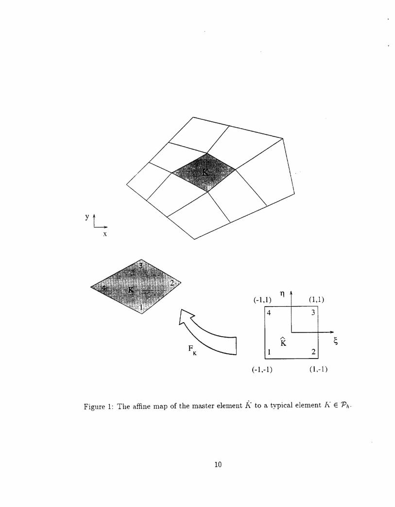
(viii) The elements !\' E Ph aTe affine maps of a master element k = [-1.1] x

[-1.1]. J\' = Ff,·(k) as illustra.ted in Fig;. 1.

(ix) Ph E F where F is a family of quasi-uniform refinements. Let hI.: =

diam(l\") and PI," denote the supremum of all spheres contained in K:

then for all Ph E F. there exist positive constants cr and T. independent

8

h d-<7 anhK -hE\' < aPK

(3)

The space of admissible solutions 1/(0.) is extended to the partition using the

broken space

II \/(K)T\'EPJ,

which admits discontinuities across element interfaces. The following notations are

used concerning functions t'. U' E \ .(Ph) :

t·- = lim v(x ± Ej3)!-o

(t', w).,.

9

x

(-1,1) 11 I (1,1)

4 3

1

(-1,-1)

A

K2

(1,-1)

Figure 1: The affine map of the master element 1\ to a typical element 1\: E 'Ph·

10

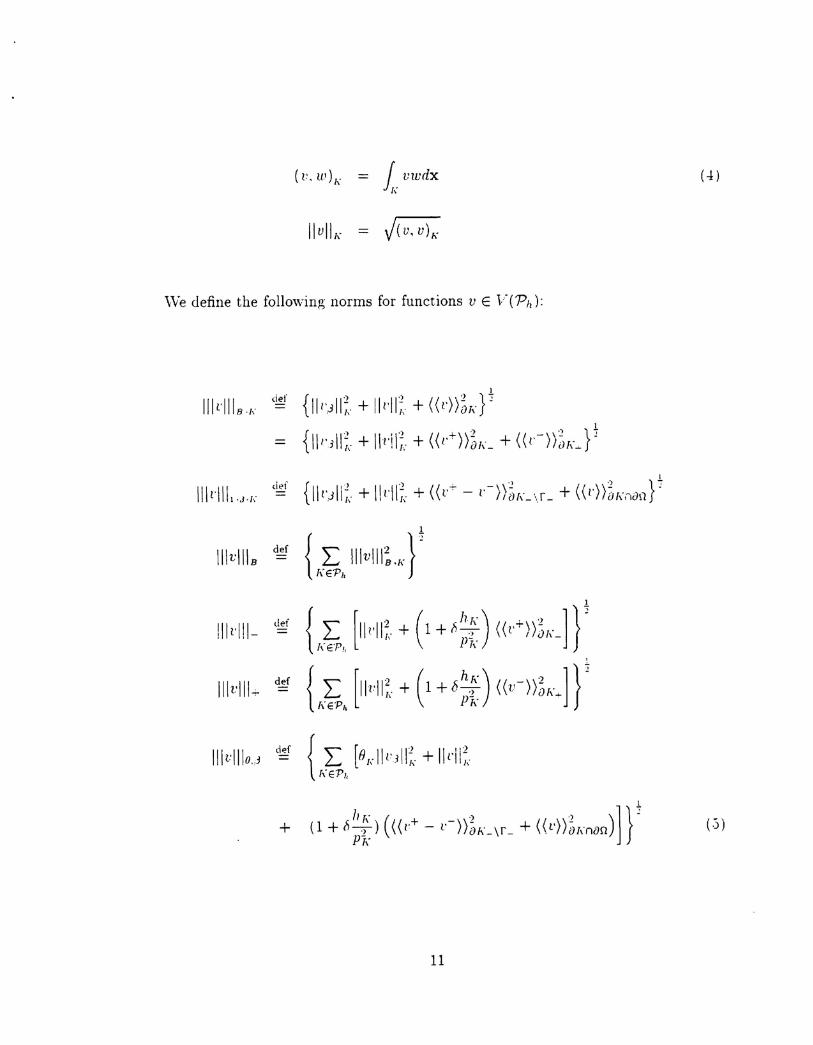
(V,W)I{ = j vwdx ( -± )I,

IIV 111\' = VCv, V)h'

\Ve define the followinl?; norms for functions v E l-(Ph):

I

Illt·llla.I" (~r {111·.311~, + 111'11;,+ ((I'))~I"rI

{II II·) II 'I'" (( +))2 (( _)\2 },- /' 3 ;,' + I'! ~: + I' iJL + l' / i)J,'~ -

I

1111'lllhJ.h <~' {1\1'.JI\;" + 111'1\;, + ((1'+ - 1'-));lL\r _ + ((1'))~I"I-liJl1r

1

111<111. ":' { L: IIIVIII~'K}'KeP"

,I.! { L [, ( hr, ) .,] r1111'111_ = " 11,-11;" + 1 + h )'2, ((vT))O!\'_I, eP"~ I I,

dd { L: [, ( h. ), ]rIllvlll.;. = 111"11;" + 1+b7 ((V-))Oh'-I-KePI. Ph

1 d., { L: [ II' I 'I'Ilvlllo.J == f11,,111'~ ~,+ \1'1 ;,'(,'eP"

11

(.j)

where D is a parameter and B is used to indicate the value of the parameter ()[\":

Iff)

Iff)

If 0

no

If I}

hKoh]) then f)r = b--:j, P"k

= hp then f) _ hI\"h" - --:jP"k

o then OK = 0

1 then H, = 1.\

The pa.rameter PI, a.ppea.ring in the definition of Of, in the mesh-dependent norm

(5) will later represent the spectral order of the polynomial approximation in I....., The

case in which the coefficient (}I, = 4p'."in (.j) plays an importa.nt role in the stahilityf{

and error of the method. as we show later.

2.3 Weak Formulation

Property (v) of the partition implies that solutions 1/ E 1/(r.!) to (1) are continuous

across element interfaces. Since the broken space a.dmits discontinuities along element

12

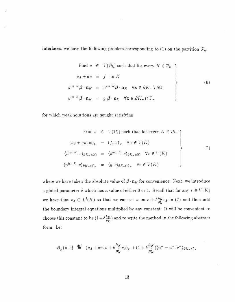
interfaces. we have the following problem corresponding to (1) on the partition Ph:

Find II E 1:'(Ph) such that for every K E Ph,

lid + all f in]{

lIextl{ f3 . Ill{ 'Vx E DIC \ DD.

q {3 . Il[, Vx E DIC n r_

(6)

for which weak solutions are sought sa.tisf~'illg

(g, V)tJLnL 'Vv E 1/( K)

\vhere we have taken the absolute value of {3. 11[," for com"enience. ::\"ext. we introduce

a global parameter c" "'hich has a value of either 0 or 1. Recall that for any l' E i"( !\")

we have that F} E L2(I\') so that \ve can set tr = l' + (s4p"L'3 in (7) and then add[,'

the boundary integral equations multiplied by any constant, It \vill be convenient to

choose this constant to be (1 + b!!.f ) and to write the method in the following abstractPl\

form. Let

13

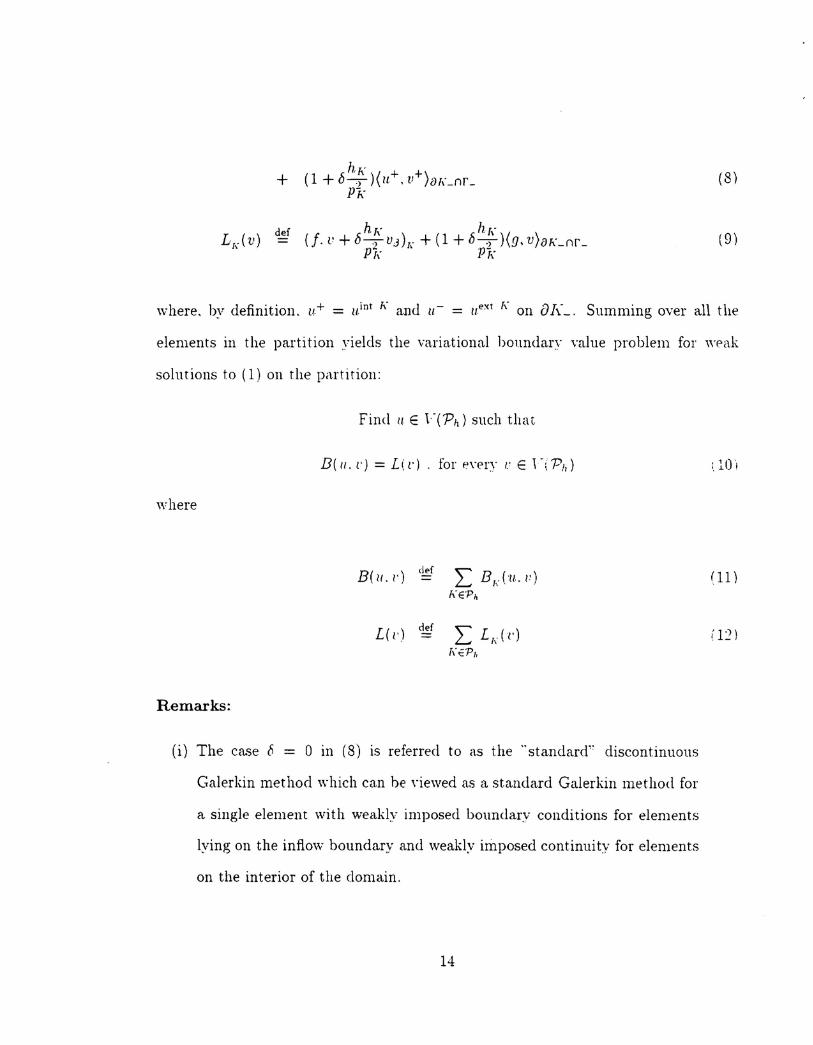
+ hTo:(1 + (j~)( u+, v+)i:JTo:_nL

P"j,:(8)

(9)

where, by definition. u+ = /lint To: and 1/- = I/ext K on fJ!\"_. Summing over all the

elements in the partition yields the variational boundary value problem for wpak

solutions to (1) on the partition:

find 1/ E F(Ph) such that.

B( II. (.) = Ii: 1') . for f:'wry c E i "(Ph)

where

:,10,

B( 1/. 1') dl'f L BiJu.· c) (11)h"EPh

I(1') dl'f L IiJd 112 )[\' ",-Ph

Remarks:

(i) The case {, = 0 in (8) is referred to as the .,standarcl" discontinuous

Galerkin method which can he "iewed as a st.andard Galerkin method for

a single element with wea.kly imposed boundary conditions for elements

lying on the inflo,v boundary and weakly irnposed continuity for elements

on the interior of the doma.in.

14

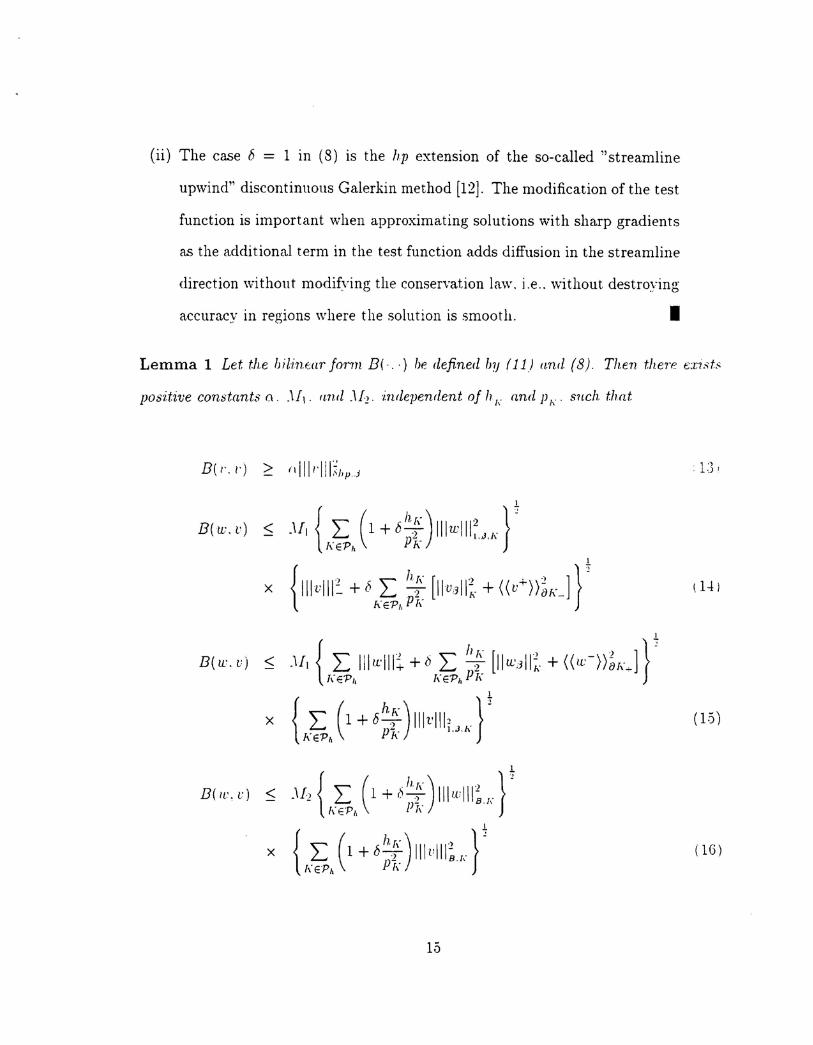
(ii) The case b = 1 in (8) is the hp ex.tension of the so-called "streamline

upwind" discontinuous Galerkin method [12]. The modification of the test

function is important when approx.imating solutions with sharp gradients

as the additional term in the test function adds diffusion in the streamline

direction without modifving the conservation law. i.e .. without destroying

accuracy in regions where the solution is smooth. •Lemma 1 Let the bilintar form B(· .. } be defined by (11) and (8), Then the7'e eruds

posdive constants (\" .\II" I/,nd -'h", i1ulepenrlent of IIF and jJ 1\' such that

B( 1". I') ~ 1I111"IIi:~hfJj • 13,

I

B(~·.t') ~ .\[, { L (1+0";')iIIWIII;,. r!\"EPh Ph

I

X {111v111: + 0 L ";'[IIUJII~+ ((V+))~I,J } , I. 1-1 j

h"EP},Ph

I

{ L' L ii, [I' ( )' ]}B(u:. vj ~ .\II IlltL'lll+ + () ""2 I tL',3II~·+ (/!.'- in'_KEPh KEPhPK

X { L (1+ o"n 111t'1I1, r (1.5)PK I.J,h

h'EPh

{ L ( /,'') I II' } jB( 1(.', v) ~ .\h 1 + (Sl":" II wi ~.I\"f\" E'P}, P f,

X { L (1 +0 ";')ill VIII~"r (16)f\" EPh P f\

15

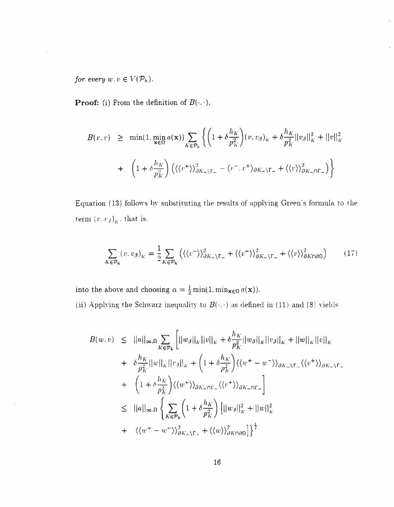
for every w.v E F(P,1).

Proof: (i) From the definition of B(·, .),

+ ( ,hT\') (( +)'2 (- +) (( ))'2 )}1 + (~pj\_ (I' )DT\'_\r_ - I' , L' iJT\'_\L + /. iJf\'_nr_

Eqnation (13) follows 1)\' substitntin~ the results of applying GrE'en's formula to r he

into the above and choosing Cl = ~min(LminxEfla(x)),

(ii) Applying the Schwarz inequality to B(·,·) as defined inl)1i and (8) ,-ields

B( w, v) ~ Iialloo,fl L [IIWJ 11K Ilvlln- + 0h~\:jlwe 11K 111',,111\' + IlwllK II vll/\!\E'Ph Ph

-h T\- I II ( 5 h T\-) (( + - )) ( ( +) )+ b ---:) IIIL' I /\ I k3 h' + 1+ (---:) Ii' - W a 1\' _ , r_ v ()L \r_Pk Pk

+ (1 + (~h~\')((n:+) )aLnr _((1'+) )aLnr_]P 1\'

< Ilal100.fl { L (1 + ohr) [llw3117\ + Ilw117,[\-E'Ph P T\

1

+ ((II'~ - 1/.' -) ) ~ L \ r_ + ((IV)) ~T\N)fl] r16

Equation (14) follows by selecting All = V2llalloo.n.

(iii) Equation (15) is obtained by applying Greens formula to the term (u:. 1:3)1{ and

(W3. U)I' in (11). and applying the Ca,llchy-Sclnvarz inequality.

(iv) Equation (16) is obraine(l by adding (1-1) and (1.5). applying the Cauchy-Schwarz

inequality to the rE"sult. and selecring -'h = 11Iallx.n.

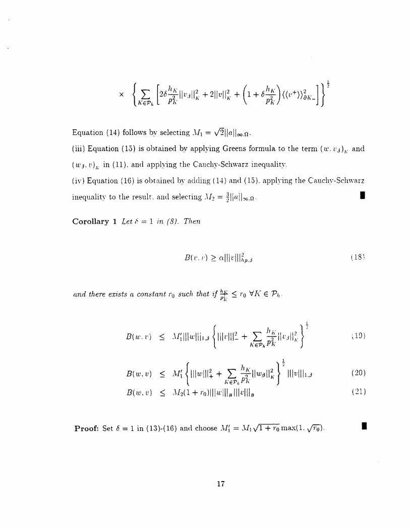
Corollary 1 Let i' = 1 in (8). Then

and there exists a constant 1'0 such that if 4p_- ~ /'0 VJ{ E Ph,I,·

•

B(w.t·) < ~la)

I

B(w,v) ~ AI~{IIIWIII~+ ?= h~IIW611~}::IIIVIII1.,3 (:20)T\ E.P" P T\

B(w, v) ~ Jh(1+ro)lllwIIIBIIIuIIIB (21)

Proof: Set {;= 1 in (13 )-( 16) and choose .M; = .\II /1 + TO max( 1. Fo)· •

17

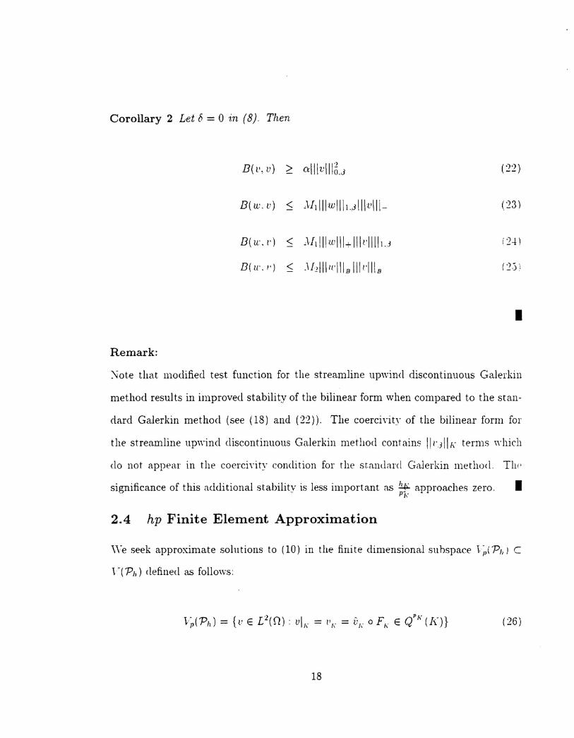
Corollary 2 Let 0 = 0 in (8). Then

B(t" u) ~ 0:11Ivlll~.3 (22)

B(w. v) ~ Jldllwlll1..3lllvlll- (23)

B(u', 1') ~ JI1!11,·ulll+llkllllu 12-!)

B(U'./·) ~ .Ihlll/['IIIBIIII·IIIB (.,. "'-') }

•Remark:

~ote that modified test function for the streamline upwind discontinuous Galerkin

method results in improved stability of the bilinear form when compared to the stan-

dard Galerkin method (see (18) and (22)). The coercivit~· of the bilinear form for

the streamline up,vind discontinuous Galerkin method contains Ik311K terms which

do not appear in the coercivity condition for the st,amlard Ga.lerkin method. Till'

significance of this additional stability is less important as 4p'_'approaches zero, •[,

2.4 hp Finite Element Approximation

\Ye seek approximate solutions to (10) in the finite dimensional suhspace 1~( Ph) C

F(Ph) defined as fo11O\\'s:

(26)

18

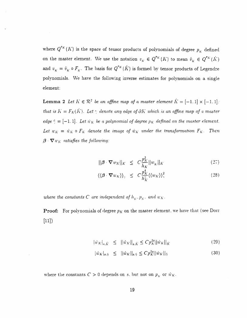
where QPr; (K) is the space of tensor products of polynomials of degree p[,' defined

on the master element. Vv'euse the notation UK E QPK (Ii..") to mean ill\ E QP[" (k)

and v 1\ = -VI,' 0 FK· The basis for QP 1\ (k) is formed by tensor products of Legendre

polynomials. vVe have the following inverse estimates for polynomials on a single

element:

Lemma 2 Let J( E R'1 be an affine map of a master element I~-= [-1. 1] x [-1. 1]:

that is !\' = F[\'(I\"). Let~, denote any edge of iJ!\' wh'ich is an affine rnap of 'I master

edge~· = [-1.1]. Let li'[\, be a polynomial of degree ]J[\' defined on the nW8ter dement.

(3 , V 1('[\' '~'at'isfies the following:

.)

11.8 . V Il'[\,11 A-Pr, P-\~ Cf-IIWh,III\' -, )tho

p-1((f3. Vwd)., l\' (( ))2 (::?8)~ CF WA- "

t'k

where the constants C are independent of hK, P,," awl U·[,'.

Proof: For polynomials of degree pr.: on the master element. we have tha.t (see Dorr

[11])

Ili·KI<.I~· ::; Ilth\·lIs.[~'::;cpk~llli~F\'lkIlh'ls.~1 ~ lith-lis.'), ~ cp*qI li'F\,II-i

where the constants C > 0 depends on .5. but not on PI; or U'''',

19

(29)

(30)

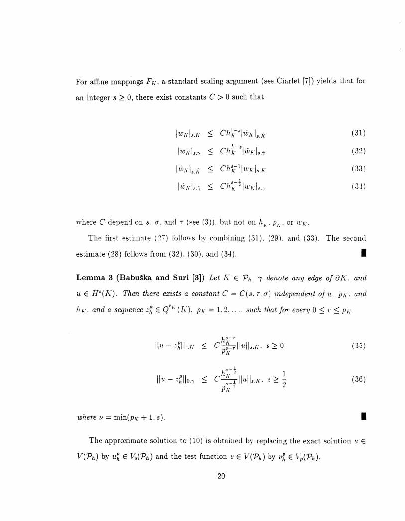
For affine mappings FK' a standard scaling argument (see Ciarlet [i]) yields that for

an integer s 2::0, there exist constants C > 0 such that

/WK!s.[,' < Ch k:-s IU'["ls.!'· (31)

!Wl\'!q 1-8< Ch},; IWh,ls.? (3:2)

l,i~[,'1 r < Ch,,-: I Ill! ["Is. I,' (33)$. \

I'l! I,'I,~,-;s-l< ChK! I n'[,' 1 .•. -,. (3-4)

\Vh!:'!'!:'C depend on s. CT. and j' (see (3)). hut not on h[". PI," or leI,'.

The first !:'stimate (~-;-) follo\\"s by combining (31), (29). and (33). The second

estimate (28) follo\vs from (32), (30), and (3-1). •Lemma 3 (Babuska and Suri [3]) Let I\- E 'Ph, , denote any edge of 81{. and

U E H8(R ..} Then there exists a constant C = C(s, T, CT) independent of u. p[,'. and

11.[,'. and a sequence .:~ E Qr[\, (K). PI\"= 1.2, . , .. such that for every 0 :::; [' :::;Pr,',

hv-r

lIlt - =::llr,K F:::; C 8~rllulls.K, 82::0Ph'

v-1I 2 1Ilu - =::110,., 1[,'

:::; C s-~ IIUlls.l\·' .s 2:: :2p f; -

where v = min(PK + 1. S).

(35)

(36)

•The approximate solution to (10) is obtained by replacing the exact solution /I. E

20

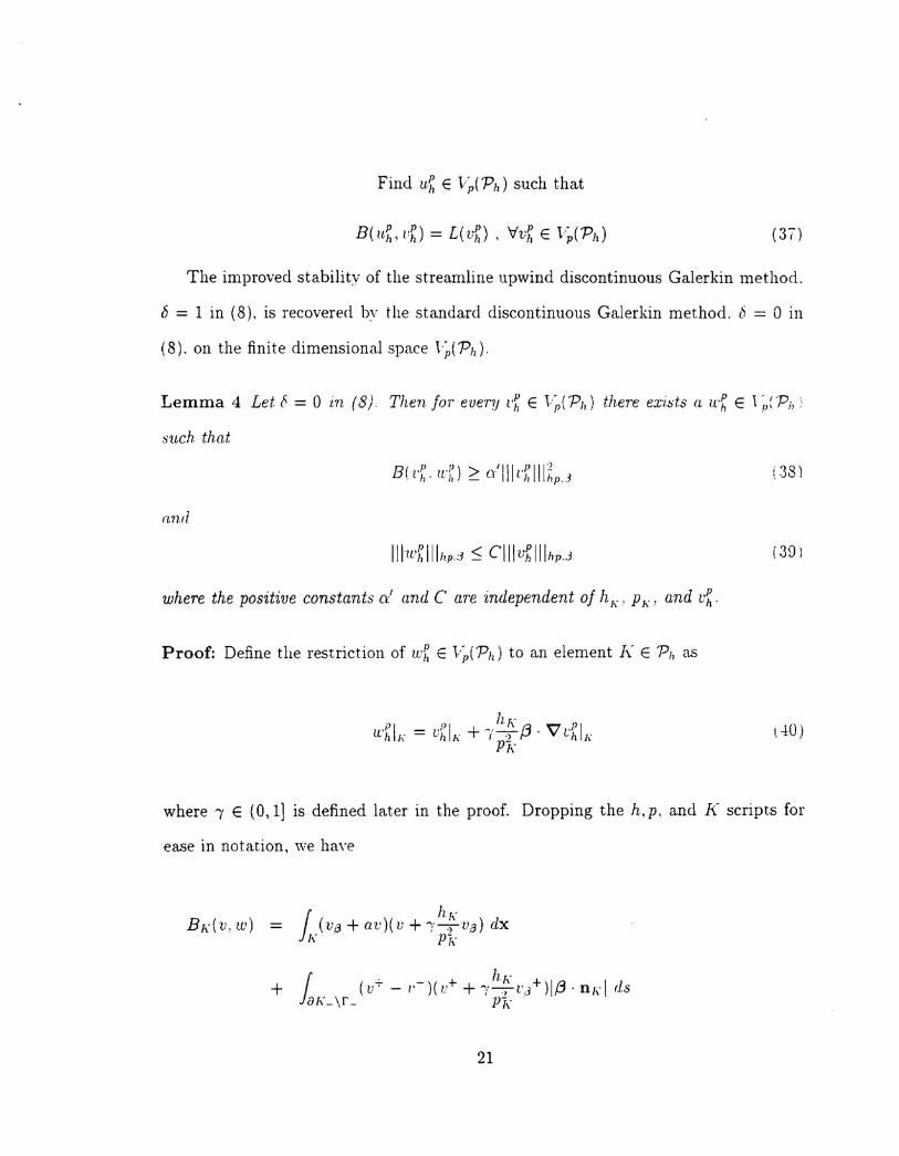
Find u~ E l'~(Ph) such that

(37)

The improved stability of the streamline upwind discontinuous Galerkin method.

b = 1 in (8), is recovered by t he standard discontinuous Galerkin method. b = 0 in

(8). on the finite dimensional space l'~(Ph).

Lemma 4 Let b = a in (8). Then for every t'f E 1;)( Ph) there ex';':;ts a It'~ E ,;)( 'Phi

stlch that

BCd:· I.L'O ~ o'llld:lllf,pj

(mil

Illw~ Illhp,] ~ C1llvh Illhp.]

where the positive constants a' and C aTe independent of hI{' PI{' and v~,

Proof: Define the restriction of w~ E l'~('Ph) to an element J{ E P'l as

(39)

\-10)

where I E (0,1] is defined later in the proof. Dropping the h, p, and !{ scripts for

ease in notation, '\ve have

B1Jv, tv) J h,,-(va + av)( v + "'(---:)va) dx

K Vk

21

I II') h{\" 1 12 1> aolv /.."+ 1-::;- Iv~1K + Vt'j3 dx

P'k h'

hI\" 1 + 2 (( .+))2+ :'-:) VVa dx + ((V ))aLnr _ + V 8K_\r_P"k K

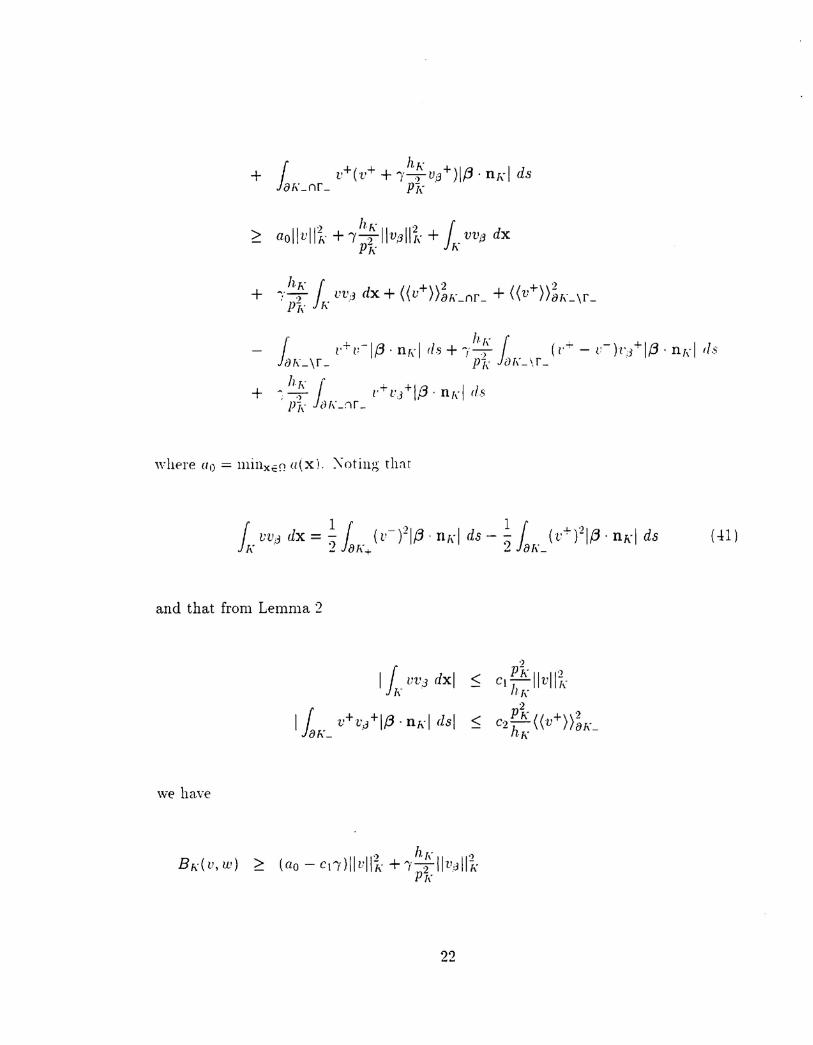
where 00 = minx.::0. u(X). \"Otillµ; th~r

and that from Lemma 2

(-11)

I r uv] dxliKI r v+v,J+I,6-nh'1 cis IJah'_

we have

22

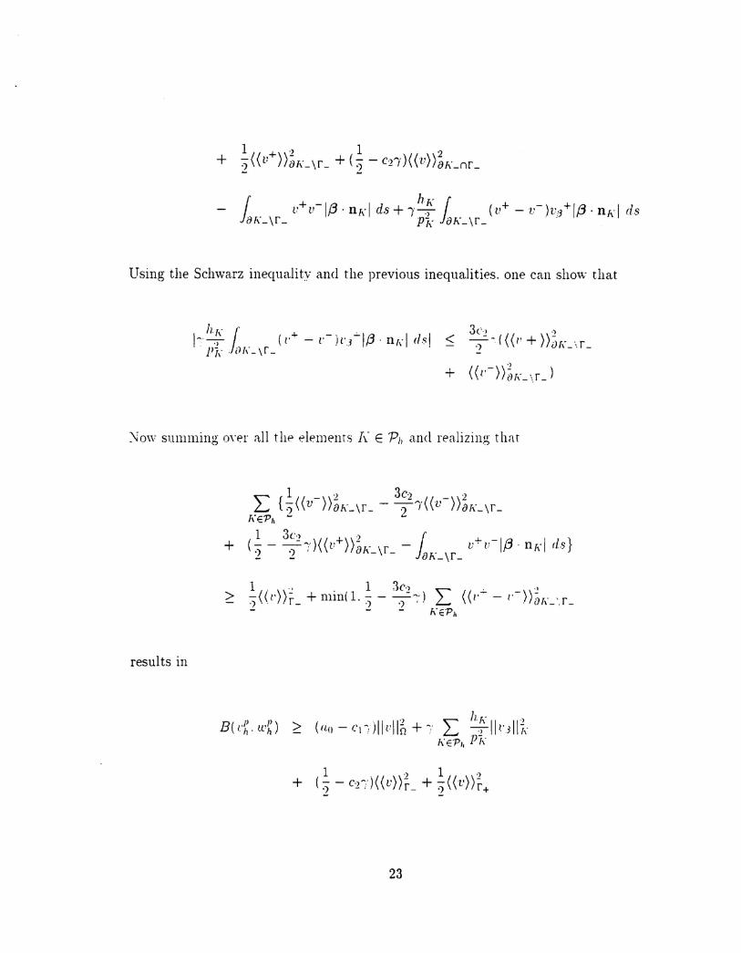
Using the Schwarz inequality and the previous inequalities. one can show that

3('·, ::!--=.-(((1' + ))iJL\r_.)

,)

+ ((I'-));:JL\f_)

:-Jow summing 0\'171' 11.11t he elements h" E Ph and realizing t har

results in

23

· 1 3C2 ~ (( + .-))2+ mlIl(L~-0;') L.. u -to D""_\L- ~ KE'Ph

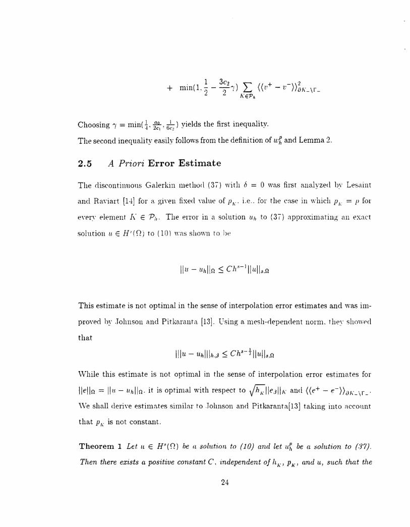
Choosing " = min( ~, ~, 6~'" ) yields the first inequality.

The second inequality easily follows from the definition of w~ and Lemma 2.

2.5 A Priori Error Estimate

The discontinuous Galerkin method (37) with () = 0 '.va.s first a,naJvzed ]n" Lesaint" ,

and Raviart [1-!] for a. giwn fixed "nIue of PI,' i.e .. for the ease in which Ph" = II for

ew'rv element X E Ph. The error in a solution 11" to (37) approxima.ting an exact

solution II E H"(D) to (10) ""as shown to Iw

This estimate is not optimal in the sense of interpolation error estimates and was im-

proved by Johnson and Pitkaranta [13]. l'sing a. mesh-dependent norm. they showpd

that

\Vhile this estima.te is not optimal in the sense of interpolation error estimates for

IJello = Ilu - 1Ihllo. it is optimal \vith respect to ~lle.3III\" and ((e+ - e-))OL\f _.

\Ve shall derive estim:1.tes simila.r to Johnson and Pitkaranta,[13] t.aking into account

that P 1, is not constant.

Theorem 1 Let II E H'«D) be rt sol1Ltion to (10) and let ui. be a solution to (.'17).

Then there exists a positive constant C, independent of hr.., PK, and u, such that the

24

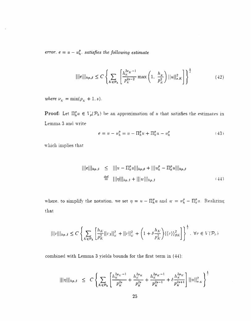
error. e = II - llft. satisfies the following estimate

where v[, = min(p i\' + 1. .s),

(42)

Proof: Let rr~II E l ;J( 'P,,) he a.n a.pproxima.tion of It. that sa.tisfies the estimat es in

Lemma 3 and write

P rrP rrp Pe = II - ll" = 11 - h II + "It - u"

"'hich implies that

Illelllhp,j ::;; Illu - rr~lllllhp.p + Illu~ - rr~lllllhp,Jdef 1111Jlllhp.J + IIlwlllhp.J

:43\

i44!

,yhere. to simplify the notation. we set '7 = 1/ - rr~It. and Ie = ([~~- rr~It. Realizing

that

combined wi th Lemma 3 yields bounds for the first term in (44):

25

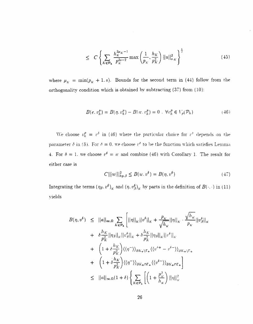
(-!5)

where µ/,_ = min(p/\. + 1. 8). Bounds for the second term in (4-1) foHmv from the

orthogonality condition which is obtained by subtracting (37) from (10):

\Ye choose uK = 1,6 in (-1.6)where the p:1,rtic1l1ar choice for 1',\ depends Oil the

parameter t~ in (8), For l~= 0, ,,-e choose 1'~ to he the functioIl which satisfies Lemllla

4. For ~ = 1. we choose (16 = Il' a.nd combine (-16) with Corollary 1. The result for

either case is

(47")

Integrating the terms ('713, u6)/\" and (1], v~)/\" by parts in the definition of B(·.·) in (11)

yields

26

11.[,' ( hE\') II 112+ 6---:') 1 + bT TJ.J KP-k PI\'

(hI\' ) .)] } ~ III 6111+ 1+ fJ pi,' (('1-))81\'+ V hp,S (-4:8)

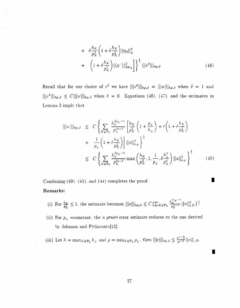
Recall that for our choice of v6 we haye IIIv6111hp,p = Illwlllhp.3 when b = 1 anel

1II1'6111hp,J ~ C1llwlllhp,3 when b = Q. Equations (48), (4';'). and the estimates in

Lemma. 3 imply that

III /('i Ilhp.3

(49)

Combining (49), ({.j). and (44) completes the proof.

Remarks:

(ii) For Pi,· =constant. the n. priori error estimate reduces to the one derived

by Johnson and Pitkar:tnta[13],

27

•

•

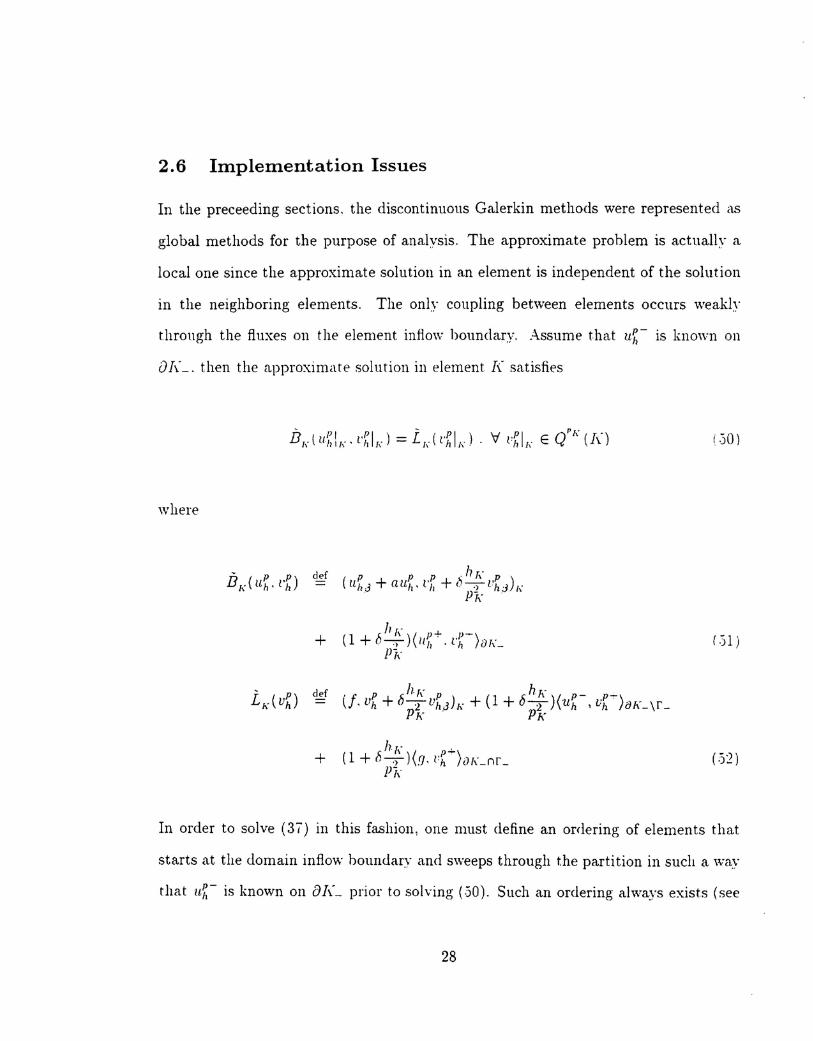
2.6 Implementation Issues

In the preceeding sections. the discontinuous Galerkin methods were represented as

global methods for the purpose of analysis. The approximate problem is actually a

local one since the approximate solution in an element is independent of the solution

in the neighboring elements. The only coupling bet\veen elements occurs weakly

through the fluxes on the element inflow boundary. Assume that lt~- is known on

01\.' __ then the approximate solution in element f{ satisfies

1.)0)

where

(.)1 )

+ ( ;52)

In order to solve (3 i') in this fashion, one must define an ordering of elements that

starts at the domain inflow boundary and sweeps through the parti tion in such a \'v'ay

that Il~- is known on DIe prior to solving (.50). Such an ordering always exists (see

28

[14]) and is fairly straightfonvard to construct. This is the optimal solution technique

for solving the linear model problem \vhere element inflow boundaries can be identified

a priori. However, an alternate approach is needed for solving nonlinear h:yperbolic

conservation laws where the fluxes depend on the solution, and thus. element inflow

boundaries cannot he identified a priori.

\Vith the aim of soh-ing more general problems in mind. the linear model proh-

lem is solved in a wav that is easily extendable to the nonlinear case. that ta.kes full

adv:Lntage of the discontinuous approxima.tion. a.nd is amenable to parallel compu-

tations: that is. by soh-ing the time-dependent conservation law for the stead,- state

solution, Sinee time aC(,1ll'al'V is not importa.nt in obtaininp; the stead~- solution. ,,-p

use the classical fon\-ard 01' backward Euler time marching \vith a truncation {'ITOI'

of O(~(!). Let 111l+1 = uf,(·.t,,+i) where tll+1 = (n + l)~t and ':::'t is the time step

increment. Assuming the solution at time tn is knov,,-n,then the fonvard Euler version

of the scheme is given by

L i lI,,-I_ 1')/, = L (uil. c),,- + ':::'t [L( l'i - I3( u" - I'l!

K ,=T'i, [,- ,=p!,

and the backward Euler version is given by

L (lI"-'-l·l')I,_ +~t L B/,(1l1l+1.1:) = L (UIl·L')I: +~t L i!,-(r) (.'5-1,)!,'E'P" !\'ET',. l,·EPI. KEPI,

To preserve the local character of the method. the inflo\v boundary terms a,ppearing

in the definition of Lr,-( 1') (see ,32) are evaluated at time level tn_

29

The initial data. ll~(" 0), needed to complete the initial-boundary-va.lue problem

IS taken to be a uniform field with a value associated with the inflow boundary

conditions.

3 A Posteriori Error Estimation

The a priori estimates derived in the previous section are useful for predicting; how

the error in numerical solutions behaws with h-refinement or p-enrichment. Cnfor-

tuna tel:\'. their usefulness in assessing the aCC1.1l'acvof ;1, gin'u numeric-al solution is

limited since the estimate involves unknown constants and the exa.ct solution we are

approxima,tinv;. :'-Jevenheless, a p.,..im"i (~nor estimates such as (·t2l and imerpolarion

errol' estimates SUell as (-1:.») have ]wen llsed ext.ensively as errol' indicators to drin'

adaptive methods for hyperholic problems [10],[19],[1::>]. Typicall,Y the unknown con-

stant is set to unity and some post-processing of the approximate solution is used in

place of the exact solution. \Vhile the element contributions to these global estimates

may provide some relative measure of the loca.l error. this approach in general fails to

provide a reliable estimate of the actual error in a particular numerical solution and

can be grossly in error.

In this section, we derive error estimates which are computed locally on a single

element and contribute to a global error estimate \....hich is a.ccurate enough to provide

a reliable assessment of the quality of the approximate solution.

3.1 Element Residual Method

The estimates derived here. based on the element residual method. are similiar to

those proposed by Bank and \Veiser [-1:] for elliptic problems and Odel1. Demkowicz,

30

Strouboulis. and Devloo [11] for solid and fluid mechanics problems, The element

residual method was extended to hp-approximations for elliptic problems by Oden.

Demkowicz, R.achowicz. and \Vesterman [16]. A global estimate of the error is ob-

tained by summing element indicators which are the solutions to a local problem with

the element residual as data. In references [17] and [16] . the local problem is of the

same form as the global problem.

For continuous finite element approximations. the element residual involves fluxes

on the boundary of an element. Since the fluxes are multi-valued. an an-raged tlux is

used. R.ecently. '-\'ins,,'orth and Oden [1]. [2] have shown that it is possible to use a

self-equilibrating ;werage flux that results in an error estimate which is equivalent to

the actua.l error :llld can be asymptotically exact for certain elliptic problems, For ;)

discontinuous approximation. the jump in the element houndary flux arises natura.lly

in the residual. eliminating the need for flux balancing,

The main difficult" with our formulation for hyperbolic conservation laws is that

the norms associated with the continuity and coercivity of the bilinear form are dif-

ferent. The use of different norms makes it impossible to construc( a single local

problem which results in an upper and lower bound of the error in the same \or an

equivalent) norm.

In the following sections. we show that it is possible. however. to construct one

local problem \vith a solution that provides a. lower bound all the actual error and

a.nother local problem with a solur.ion that provides a.n upper hound on the actual

error. \Ve a.lso show that a local problem based on the origina.l problem results in a

10callO\ver bound. \Ioreover. if the approximation of the solution to this local problem

is limited to a certain class. then the estimate is equivalent to another common Iv used

31

approach: estimating the error as the difference between a newly contructed (and

hopefully more accurate) solution and the approximate solution on hand.

3.2 A Global Lower Bound on the Error

A local problem is constructed which results in a lower bound on the error in a sense

to be defined precisely later. Letlt]\_ E QPK (K) denote the approximate solution in

an element I': and -; h- E 1'(1\') be the solution to the following local problem_

(.j,) )

and a > 0 is a constant. Then

induces a norm on F( Ph) which will be referred to as the A L -norm:

( ,58)

32

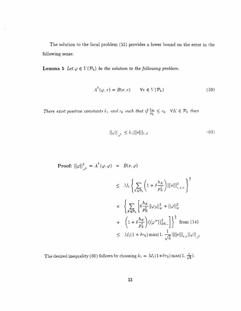
The solution to the local problem (55) provides a lower hound 011 the error in the

following sense.

Lemma 5 Let..p E F(Ph) be the solution to the following problem:

LA (;p, v) = B(e, l!) (59)

There exist positwe constants kl flnd"ll 81/ch that i] !!..K.pl~' -:; I'll V!\- E Ph then!\

IGO)

B(e, :p)

The desired inequali ty (60) follows hy choosing k 1 = :H] (1+6 fa) max( 1,*).33

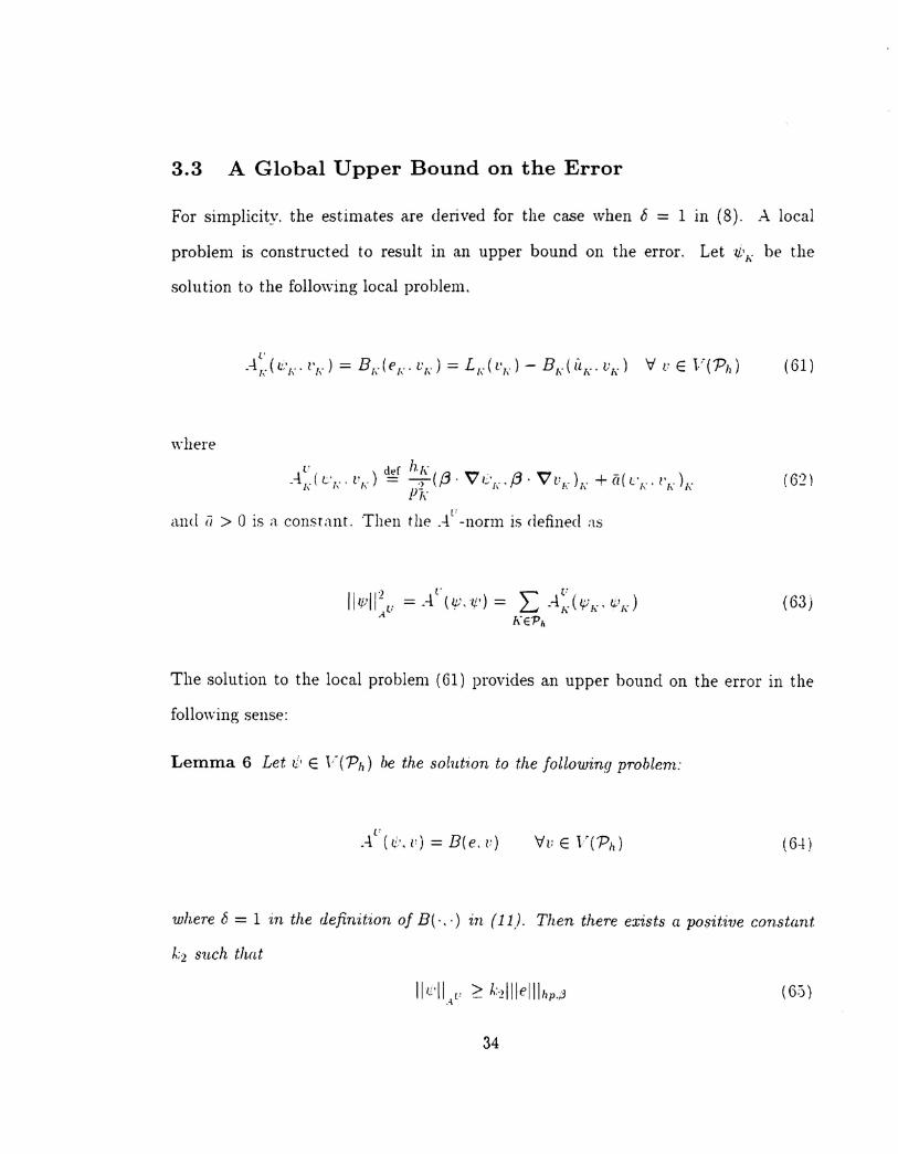
3.3 A Global Upper Bound on the Error

For simplicity. the estimates are derived for the case v,,-hen b = 1 in (8). A local

problem is constructed to result in an upper bound on the error. Let "/l'1\0 be the

solution to the follO\ving local problem,

where

F , ) d~f h h"" _A10( C·To. vlo = --:;-({3. VC·lo,{3. Vv/o )T" + a( CTo.I'To )1'\ \ \ j)]\" \ \ \ '\ \ \.

and i.i > 0 is a constant. Then the .-( -norm is defined as

(62)

(63)

The solution to the local problem (61) provides an upper bound on the error in the

follO\ving sense:

Lemma 6 Let Ii' E "(Ph) be the solution to the following problem:

('

A, (Ii', 1') = B( e. u) (6-l)

where b = 1 in the defindion of B(·,·) in (11). Then there exists a positive constant

1.:2 such that

(6:))

34

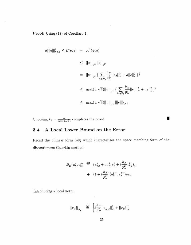
Proof: Using (18) of Corollary L

o:lllelll~p,;3 ~ B(e.e)u

A. ('~'. e)

< 111['11./; Ilell.4U

< max(l. JaHlcll,4u IIJelllhp.3

Choosing k.) = (():!'_' completes the proof.'.- - max .vQ)

3.4 A Local Lower Bound on the Error

•Recall the bilinear form (.30) which characterizes the space marching form of the

discontinuous Galerkin method:

Introducing a local norm.

35

(66)

and using Green's formula, it is easy to shmv that there exist a constant C > 0 sllch

that

:'-Jawconsider the following local problem:

B"k[" 1',,) = B[,(f[,.l'" ) . til'" E l'(h')h ' \ 1\' \ \ .\' .\

then.; [, provides a local lower bound on the error in the following sense,

(6;-)

(68)

Lemma 7 Let 'PK E V(K) be the solution to (68). Then there exists a constant

1.:3 > 0 such that

(69)

Proof: Setting 1'[, = y;,' in (68) and using (6;-) yields

(,0)

Setting ,11["= max( L Ilull?G,/,. ) and applying Young's inequality, ((f> :::; ta2+F.l)2, f > O.

to each term in BJ, ( e K . '?K) yields

(71)

36

Selecting E < 2.0[\ in (/l) and combining with (70) completes the proof.

3.5 Approximation of the Local Problems

•An approximate solution to the local problem measured in the corresponding norm

serves as a local error indicator for an element. Since the discontinuous Galerkin

solution satisfies the orthogonality condition.

(-;-2)

we must approximate the error indicator with a polynomial of (legreE' P;.: + rJ";,- whe!'l:'

tJ[,- ~ 1 in order for the discrete local problem to have a 1l00Hri\'ial solutiOl:. If a

complete polynomial of degree P [,'+ rJ" I,' (on the master element) is used to approximate

the solution to the local problem, then the discrete local problem requires the solution

of a system of order (PI\ + rJ"I, + 1)2 This system can be fairly large .compa.red to

the system of order (PK + 1)2 equations used to obtain the approximate solution for

which we are estimating the error_

Since (PI\" + 1)2 terms on the right hand side of the discrete local problem (cor-

responding to (.2)) are zero. we can make a simplification by approximating the

solution to the local problem in the space QP/\+O'/\ (K) \ QP/\ (K). In other words, the

solution to the local problem can be approximated with incomplete polynomials of

degree PI,' + rJ"[,' by neglecting the terms associated with polynomials of degree Ph--

This simplification results in a system of (Jl\( (J I\" + 2p K +2) equations for each element.

The size of the local problem can be further reduced by approximating its solution

using only the "]mhble" functions in the enriched space denoted hy Q~I,-+ITI'-(l\-) \

37

Q~/\ (K). These are the polynomials in QPr,-+u/\ (J{) \ QPr-.: (1() which are zero on

the boundary of an element. This additional simplification results in a system of

a!,' (a r-.: + 2p J\ - 2) equations which is smaller than system of equations used to obtain

the approximate solution.

3.6 Remarks Concerning an Alternate Approach

Suppose that an a.pproximation [- to the exact solution II can he constructed which

is more accura.te than the approximate solution on hand. u;~_Then a simple estimate

of the error. e = II - u~ = n - [: + C- - I/;~.is fI = II C - 1tf.11 \vhere II . II is any sui t ahle

norm. esing the triangle inequality. we have

Ilell - lIu - C11 ~ f} ~ llell + Ilu. - nl

or equivalentlyJJu - U11 B lIu - U1J

1- "" ~~~1+

If Ilu - U11 « lIell = lin - rl~lI· then e = jW - uf.11 is a. goon error estimatt>

with an effectivity index, 11:11' near unity. The main difficulty wit.h this approach

is to efficiently construct such aU. One obvious strategy for constructing a more

accurate approximation, U, is to re-solve the approximate boundary-value problem

on an enriched space.

For continuous finite element approximation~. t.his leads to a global system of

equations that is much larger, and therefore much more costly to solve. than the

original problem. For a discontinuous approximation. re-solving the problem on a.n

enriched space of complete polynomials is still more costly than the original problem.

38

but is no more costly than solving the local problems in section 3.2-3.4 on the complete

polynomial space.

The computational cost of this approach can be further reduced by "freezing" the

lower-order solution and re-solving the problem on an incomplete polynomial space

of bubble functions. In other \vords, let UI\ = 1l~11\ + wl\ v,,'here wI\' E Q61"+0"1\' (l\') \

Q6l\' (J{) satisfies

In this case. the error estimate is H = IIF - u~11= Illl'll, \Tote that this is equiya.lenr

to solving the local problpm (68) 011 the space of 1mbble functions. \Ye remark that

Peraire and ~\lorgan [20] simply post-process the a.pproximate solution to obtain the

degrees-of-freedom (higher-order derivatives) corresponding to the bubble functions,

4 Numerical Examples

The discontinuous Galerkin methorl is used to solw several examples to writ\- the (/.

priori error estimates derived in Section 2 and to investigate the performance of the

the a posteriori error estimates of Section 3. The performance of the error estimate

is measured by the effectivity index which is the ratio of the estimated error to the

actual error in the same norm. A reliable estimate is Olle for which the effectiyity

index is near unity.

R.esults are presented for the final mesh obtained using an hp-adaptive strategy

developed by Odell, Patra, and Feng [18] for a large class of elliptic problems and

extended to discontinuous solutions of hyperbolic problems by Bey [.j]. The II p-

39

adaptive strategy is based on a reliable a posterior£ error estimate for determining

the error in the approximate solution and an a priori error estimate for determining

hmv to modify the mesh to improve the solution accuracy to a specified level. The

goal of the hp-strategy is to deliver a solution with a specified error in only three

steps:

(i) Construct an initial partition Po containing N(Po) elements. The ele-

ments in Po can he of uniform P [,. = Po and essentially uniform in II. /\' = II 0)'

Solve the problem of interest on ,~)o(Po) and estimate the error.

(ii) Construct a pa,rtition PI hv suhdividing ea.ch element in Po into the num-

ber of elements required to equi-distrihute the error and relluce it to it

specified level. Solw the problem on l(~o(PI) and estimate the error.

(iii) Enrich the approximation space by increasing PI\" for every 1.....- E PI m

such a way to equi-distribute the error in smooth regions and reduce it to

the specified level. Solve the problem on the enriched space l'~l(PI) and

estimate the error.

Complete details of the IIp-adaptive strategy and other numerical results can be found

in reference [5].

4.1 Example 1

The linear model prohlem (1) is soh'ed with the following data:

(i) D = (-1. 1) x (-1.1)

(ii) {3 = (0.8, 0.6(

40

II!

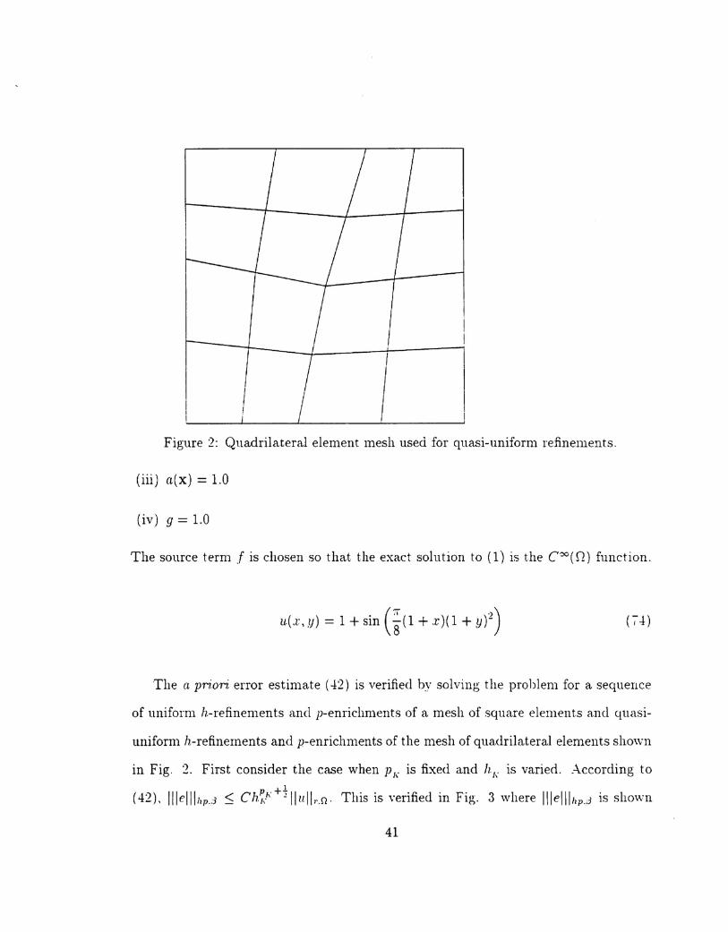
Figure 2: Quadrilateral element mesh used for quasi-uniform refinements.

(iii) a(x) = 1.0

(iv) 9 = 1.0

The source term .f is chosen so that the exact solution to (1) is the CX,( 0.) function.

u.(x,.1)) = 1+ sin (i(l + .r)(l + y)2)

The a priori error estimate (42) is verified by solving the problem for a sequence

of uniform h.-refinements and p-enrichments of a mesh of square elements and quasi-

uniform h-refinements and p-enrichments of the mesh of quadrilateral elements shown

in Fig. 2. First consider the case when PK is fixed and 11./\, is varied. According to

(42), 1IIeIIIIlP.:3 ::; Ch~f\+!llllllr.n. This is verified in Fig. 3 where 111e111hp.3 is shown

41

10"

10"

10'"

IIlelll....~

10~

10"

10"

--

- square elements

- - - - - . quad elements

/ _,'/14.5,,/ "LJ

•• ' 1

10'h

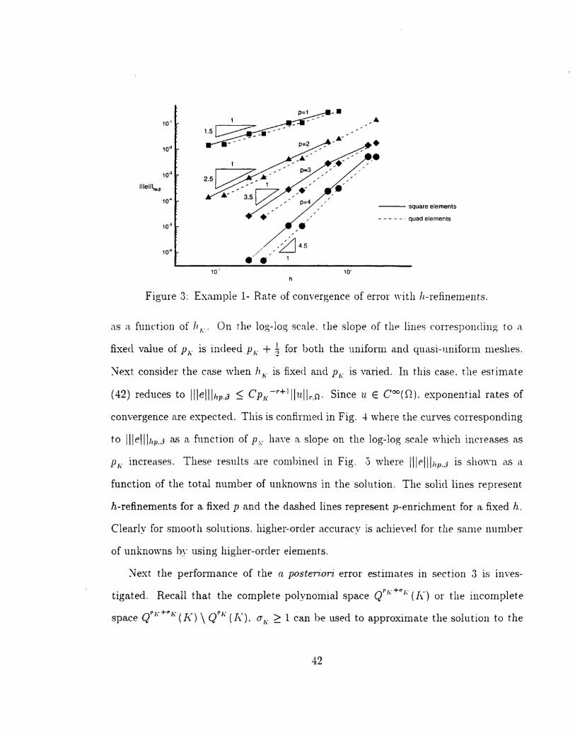
Figure 3: Example 1- Rate of convergence of error with !I-refinements.

as a function of II!,.. 011 the log-log scnle. the slope of the linE'Scorresponding to a

fixed value of Pf{ is indeed p!, + ~ for both the uniform and quasi-uniform meshes.

:'-Jext consider the case when 11f{ is fixed and Ph' is varied. In this case. the estimate

(42) reduces to Illelllhp.J ~ CPK-r+lll1t.llr,fl. Since u E COO(D}. exponential rates of

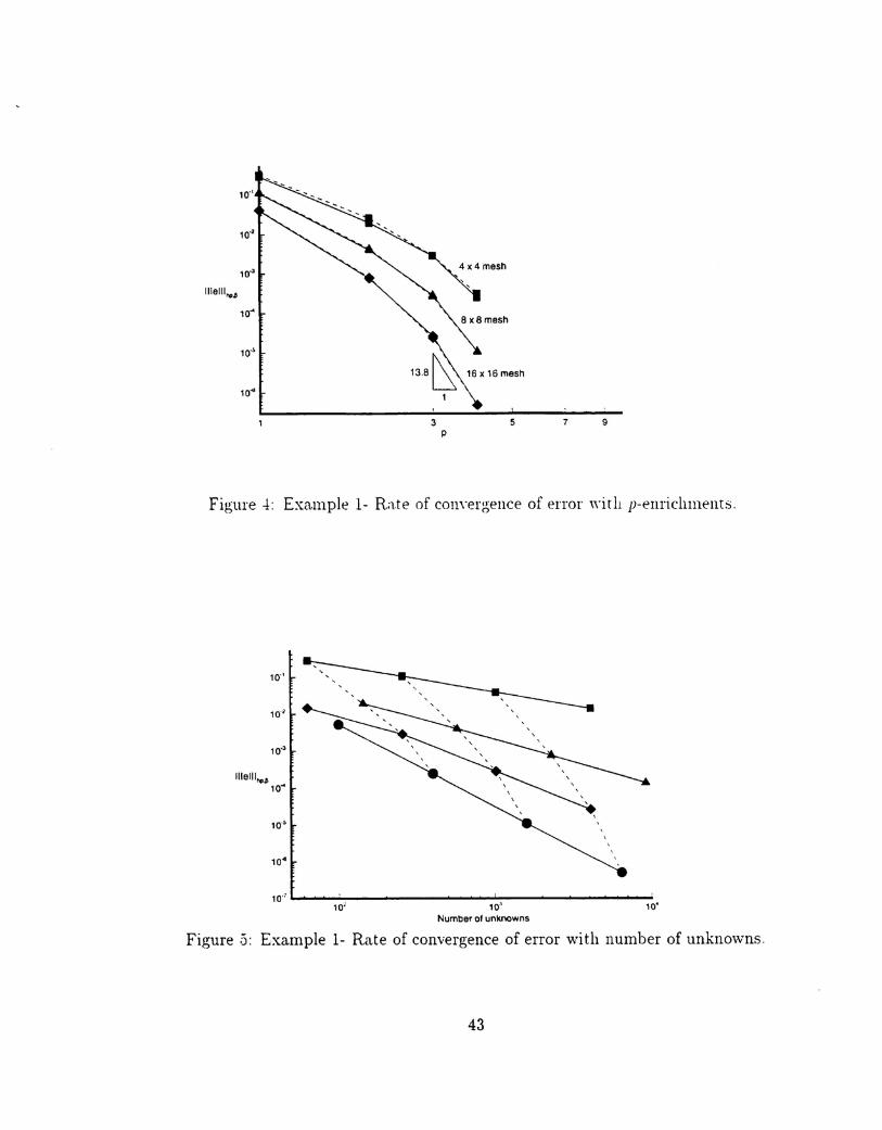
convergence a.re expected. This is confirmed in Fig. -! where the curves corresponding

to Illelllhp.J as a function of PI,' ha,\-e a slope on the log-log scale which increases as

Ph' increases. These results are combined in Fig. ;j where Illplllhp.J is 5110\\'11as a

function of the total number of unknowns in the solution. The solid lines represent

h-refinements for a fixed p and the dashed lines represent p-enrichment for a fixed h.

Clearly for smoot h sol utio11s. higher-order accuracy is achieved for the same number

of unknowns by using higher-order elements.

~ext the performance of the a posteriori error estimates in section 3 is inves-

tigated. Recall that the complete polynomial space QP!" +"K (1\-) or the incomplete

space Q"!"+"K (J{) \ QI'/,. (1\'). UK ~ 1 can be used to approximate the solution to the

42

IIlelll ....~

3P

7 9

Figure -!: Exa.mple 1- Rate of COll\-ergence of error \\'itll p-enriclnuents.

10"

lIIelll ....~ ..10

10"

10' 10'Number of unknowns

10'

Figure 5: Example 1- Ra.te of convergence of error with number of unknovms.

43

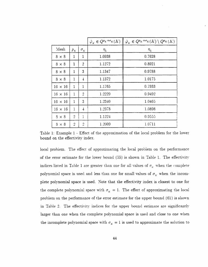
.; h' E QPh' +u K (K) .ph' E QP h' +u K ( K) \ QP h' (1{)

:\:Iesh Ph' aI, 'h, ''lL8 x 8 1 1 1.0938 0./628

8 x 8 1 2 1.1272 0.8921

8 x 8 1 3 1.1347 0,9/88

8 x 8 1 4 1.1372 1.017.j

16 x 16 1 1 1.1/65 0,'/933

16 x 16 1 .) 1.2220 0.0402 !

16 x 16 1 3 1.2340 1.046.)

16 x 16 1 4 1.23/8 1.0898i S x S .) 1 1.1224 0,0:)·).)I - I i

S x 8 .) .J 1.2000 1.0/11I,i

Table 1: Example 1 - Effect of the approximation of the local problem for the lowerbound on the effectivity index.

loca.l prohlem. The effect of approximating the local problem on the performa.nce

of the error estimate for the lo\ver bound (.35) is shmvn in Table 1. The effectivity

indices listed in Table 1 are greater than one for a.ll '"allieS of ai,' when the complete

polynomial space is used and less than one for small values of aI, when the incom-

plete polynomial space is used. Note that the effectivity index is closest to one for

the complete polynomial space \vith a/,' = 1. The effect of approximating the local

problem on the performance of the error estimate for the upper hound (61) is shown

in Table 2. The effectivity indices for the upper bound estimate are significantly

larger than one when the complete polynomial space is used and close to one vv"hen

the incomplete polynomial space with ah' = 1 is used to approximate the solution to

44

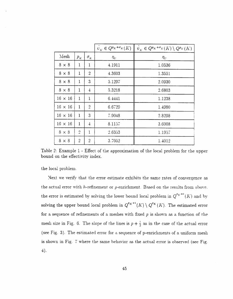
t:.~'KE QPK+O'/\ (1() J'K E QPK +"/\ (1\-) \ QP[, (1()

:vIesh Pi, U[," flu 'h,

8 x 8 1 1 4.1911 1.0536

8 x 8 1 2 4.3603 1.3551

8 x 8 1 3 5.1297 2.0930

8 x 8 1 4 .).3218 2,6803

16 x 16 1 1 6,-1441 1.1238

16 x 16 1 .) 6,6729 1.4980

16 x 16 1 3 7,9048 2,8298 !16 x 16 1 4 8. l1;j/, 3,6008 I8 x 8 I ~ 1 I :2 ,63.j3 1. H);) I !

!

8 x 8 .) 2 3,7052 1.401:2

Table 2: Example 1 - Effect of the approximation of the local problem for the upperbound on the effectivity index.

the local problem.

~ext we verify that the error estimate exhibits the same ra.tes of convergence as

the actual error with fl.-refinement or p-enrichment. Based on the results from abow.

the error is estimated by solving the lower bound local problem in QPl.;+1 (1\.") and by

solving the upper bound local problem in QPK+1 un \ QPl\" (]{). The estimated error

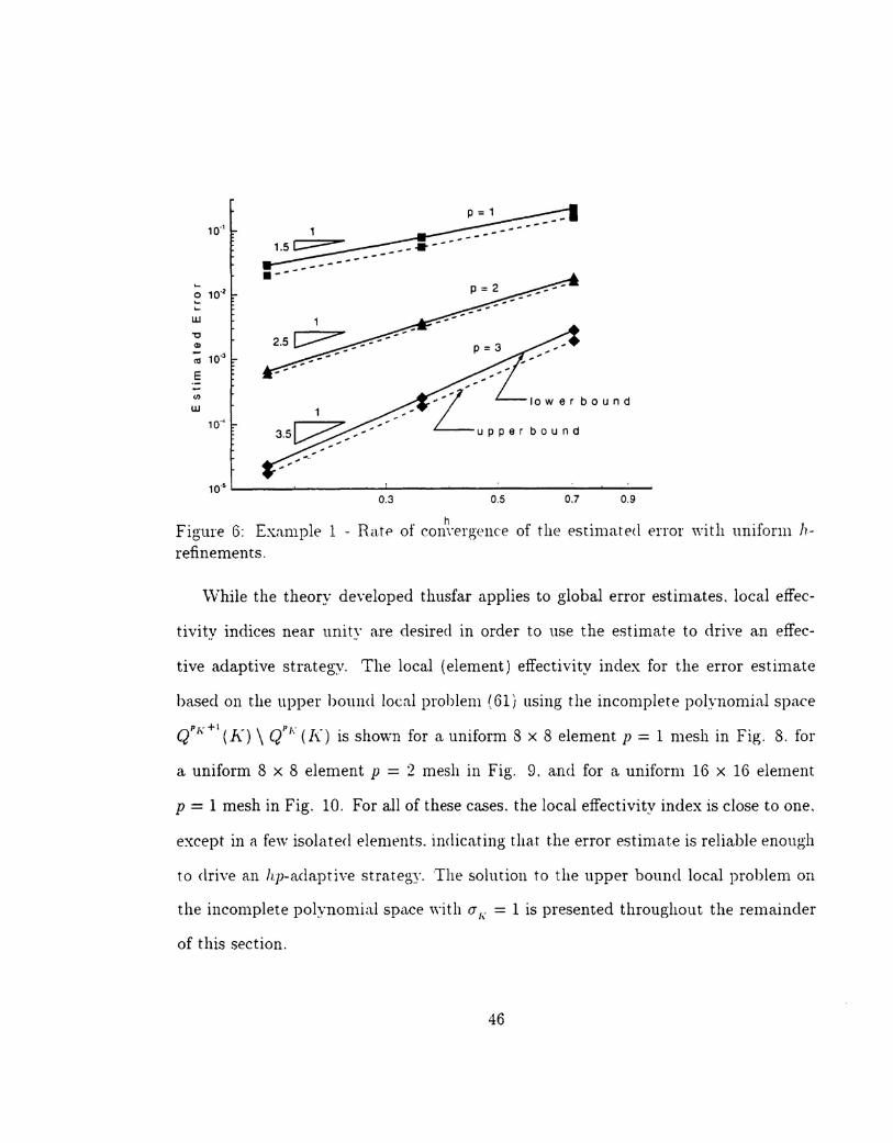
for a sequence of refinements of a meshes with fixed p is shown as a function of the

mesh size in Fig. 6. The slope of the lines is P + j a.<;in the ca.'3eof the actual error

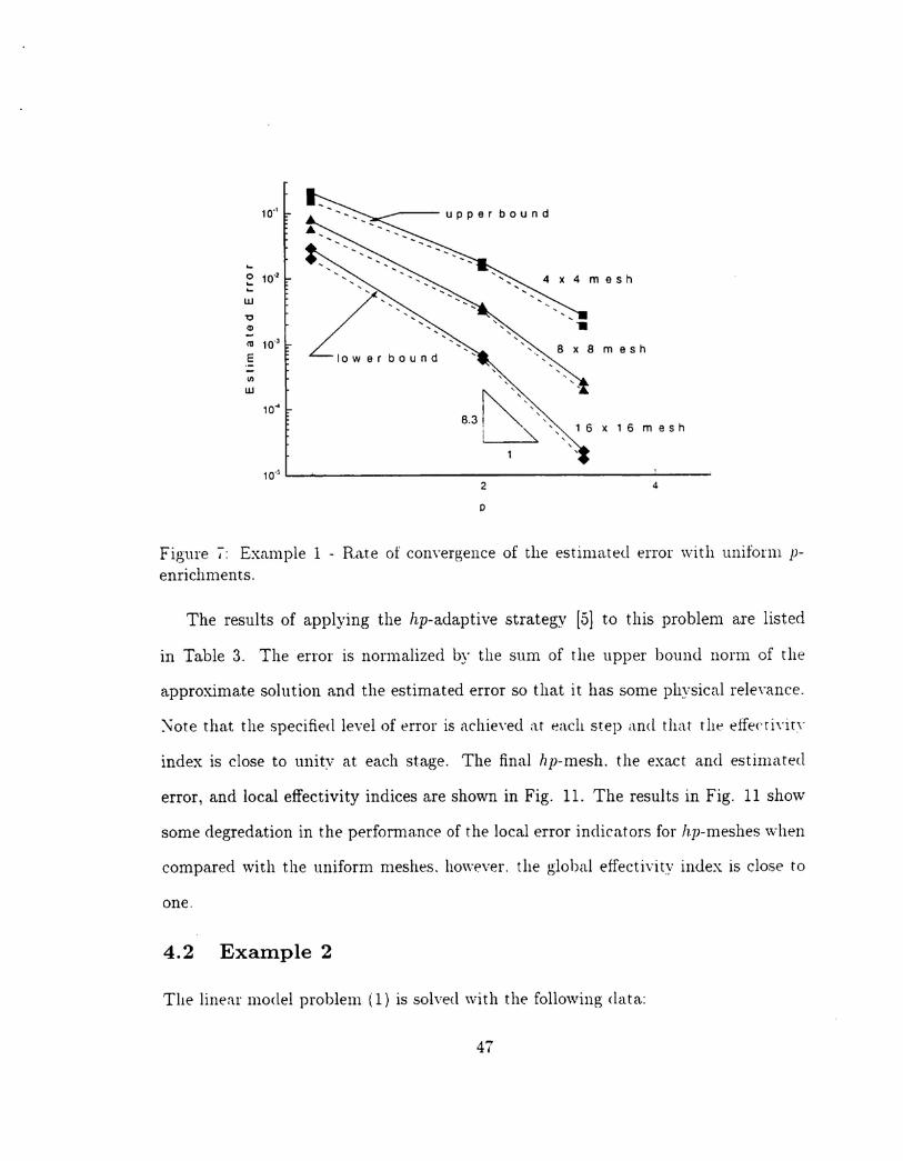
(see Fig. 3). The estimated error for a sequence of p-enrichmenrs of a uniform mesh

is shown in Fig. /' where the same behavior as the actual error is observed (see Fig,

4).

45

0.3 0.5 0.7 0.9

Figure 6: Example 1 - Rat!> of cOI~'ergellce of the estimated error with uniform h-refinements,

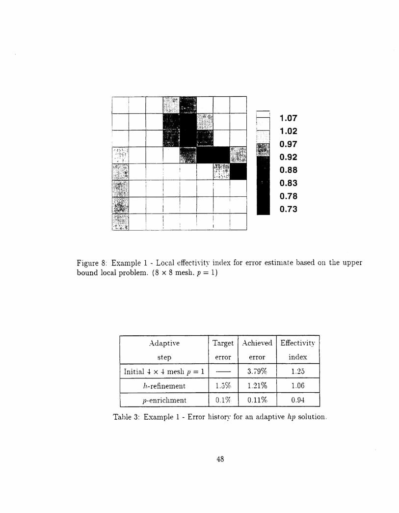
\Vhile the theory developed thusfar applies to global error estimates, local effec-

tivity indices near unity are desired in order to use the estimate to drive a.n effec-

tive adaptive strategy. The local (element) effectivity index for the error estimate

based on the upper bound local problem (61) using the incomplete polynomial spa.ce

QPb:+1

(K) \ QPj.: (K) is shown for a uniform 8 x 8 element p = 1 mesh in Fig. 8. for

a uniform 8 x 8 element p = 2 mesh in Fig. 9, and for a uniform 16 x 16 element

p = 1 mesh in Fig. 10. For all of these cases, the local effectivity index is close to one,

except in a fe,,,,isola ted elements. indicating tha.t t.he error estimat.e is reliable enough

to drive an hp-adaptive strategy. The solution to the upper bound local problem on

the incomplete polynomial space with (7/.; = 1 is presented throughout the remainder

of this section.

46

upper bound

w

EIII

W

10"

2

D

m e s h

m e s h

x16mesh

4

Figure 7: Example 1 - Rate of conyergence of the estimated error with uniform p-enrichments.

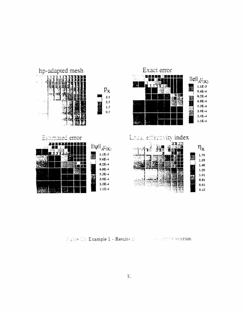
The results of applying the hp-adaptive strategy [5] to this problem are listed

III Table 3. The error is normalized by the sum of the upper bound norm of the

approximate solution and the estimated error so that it has some physical releyance.

~ote that the specified level of error is achieyed a.t each step and that the effeerivin"

index is close to unit:v at each stage. The final hp-mesh. the exact and estimated

error, and local effectivity indices are shown in Fig. 11. The results in Fig. 11 show

some degredation in the performa.nce of the local error indicators for hp-meshes \vhen

compared with the uniform meshes. however. the global effectivity index is close to

one.

4.2 Example 2

The linear model problem (1) is solved with the following data,:

47

I 1ni\1; .... I

1.071.020.970.920.880.830.780.73

Figure 8: Exa.mple 1 - Local effectivity index for error estimll,te based on the upperbound local problem. (8 x 8 mesh. p = 1)

Adaptive Target Achieved Effectivity

step error error index

Initial 4 x 4 mesh p = 1 - 3.79% 1.)-._v

h- refinemen t 1.5% 1.21% 1.06

p-enrichment O.ll~ 0.11% 0.94

Table 3: Example 1 - Error history for an adaptive hp solution.

48

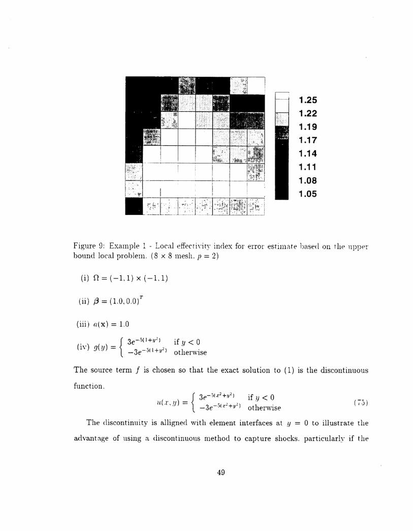
1.251.221.191.171.141.111.081.05

Figure 9: Example 1 - Local effecti\"ity index for error estimate hased on the upperbound local problem. (8 x 8 mesh. p = 2)

(i) O=(-l.l)x(-l.l)

(ii) f3 = (1.0, O.O{

(iii) a(x) = 1.0

{

3e-·,)(I+.,,~) ify<O(iv) g(y) = _3e-j(l+y2) otherwise

The source term f is chosen so that the exact solution to (1) is the discontinuous

function.

{3e-)( x2 +y") if ,1) < 0

1/.(.1', y) = -3e-)('1'~+Y") otherwise (-;-.j)

The discontinuity is alligned '''''ith element interfaces at ,lj = 0 to illustrate the

advantage of using a discontinuous method to capture shocks. particularly if the

49

'.

;:>,

.. '.. ". "':.; " .. ", "

<- ,.~;

, I .. ··. ~

I--

.-I

!.~ I,

I i I~~ I

I I I IJ I I I I I I

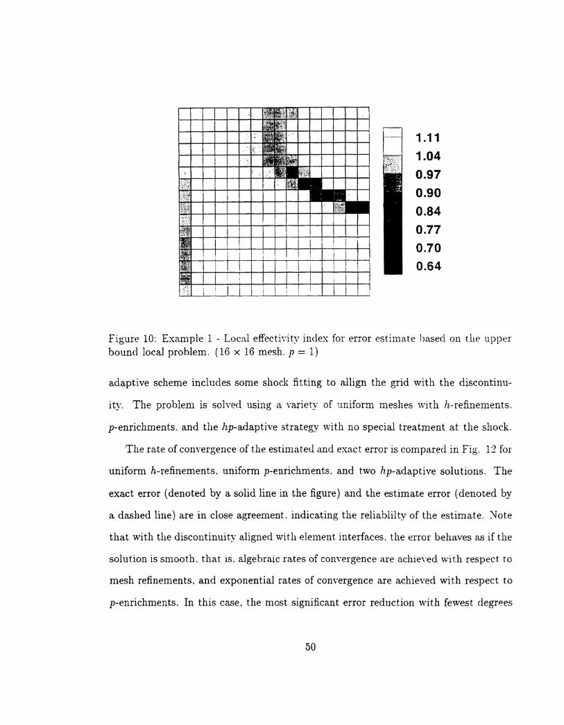
1.111.040.970.900.840.770.700.64

Figure 10: Example 1 - Local effectivity index for error estimate based on the upperbound local problem, (16 x 16 mesh. p = 1)

adaptive scheme includes some shock fitting to allign the grid with the discontinu-

ity. The problem is solved using a. variety of uniform meshes ,vith h-refinements.

p-enrichments. and the hp-adaptive strategy with no special treatment at the shock.

The rate of convergence of the estimated a.nd exact error is compared in Fig, 1:2 for

uniform h-refinements. uniform p-enrichments. and two hp-adaptive solutions. The

exact error (denoted by a solid line in the figure) and the estimate error (denoted by

a dashed line) are in close agreement. indicating the reliablilty of the estimate. :-lote

that with the discontinuity aligned with element interfaces. the error behaves a.s if the

solution is smooth. that is. algebraic rates of convergence are achieved with respect to

mesh refinements, and exponential rates of convergence are achieved with respect to

p-enrichments. In this case. the most significant error reduction with fewest degrees

50

hp-adapted mesh'1'1']'1 1T':i~:J1J1I1I1I

_ ;.nJJ 'Jl]lM:r.l~JJlJI.

"'1~~' ,~:s,,'II'S~.Jill' lZ~:' '~~~:',.". ~ .- . . ,I,.. ,.. ~ ., I -. ,,': ,- :t,t '] lJ••

i"'=" '''''~3,'- )I••

-j '.l~Y·~';:1··-i~-I" -I··I ;;1'I ~~1'

- ,--i '~i1:mD_:.:.,~?n"n

... J :;;J~.u

PK

"

3,=,

I~:;, 0 ..

IlellAU(K)

• 1.1E-3., 9.6E-~

8.:!E-~

6.8E-~=,,3E-~3,9E-42.5£-41.1E-4

1.1E·4

2.5E-4

1.791.59

1.40

1.20

1.01

0.81

0.61

0.42

1.1E-3

9.6E-48.2E·~6.8E-4

'fi"4 ='.3E-43.9£-4

.- ":',:~ .. ' Example 1 - Res1..:1t':: , -" ''-',l:tlon.

IIell"u 10.1

exact

estimate

h-refinement ; ~p;;;;3~

Number ot unknownsFigure 12: Example:2 - Rate of convergence of the error with respect to the totalnumber of unknowns.

of freedom will result by specifying a target error for the h-step which is closer to the

initial error than to the final target error. This is verified by two curves corresponding

to two hp-adaptive solutions in Fig. 12. The error history for the hp-adaptive solution

starting with an 8 x 8 mesh of p = 1 elements is listed in Table -1:. Results on the

final mesh are shown in Fig. 13. Poor local error estimates are observed in the two

parallel vertical regions indicated by the darker shades in Fig. 13. Moreover, the local

error is significantly underestimated in these regions. This under-estimation is also

present after the h.-refinement step of the adaptive strategy, This under-estimation

is possibl:v due to a failure of the procedure to adequately handle the very high

changes in gradients in these regions. The glohal effectivity indices. however. a.re

quite satisfactory with effectivity indices very near unity as listed in Table -1.

11'V11,.F(K)

I 3.SE-33.1E-32.6E-32.2E-31.8E-3l.3E-38.8E-44.4E--I

11K11.641.44

I I 1.23

1.030.830.630.430.23

53

Adaptive Target Achieved Effectivity

step error error index

Initial 8 x 8 mesh. p = 1 - 15.4% 0.998

h-refinement 7.5% 3.3% 0.996

p-enrichment 0.3% 0.55% 0.901

Table 4: Example 2 - Error history for an adaptive hp solution starting with a uniform8 x 8 mesh, p = 1.

4.3 Example 3

The following data is used in (1):

(i) O=(-1.1)x(-1.1)

(ii) f3 = ('v'2 V2)T:2 ' :2

(iii) a (x) = 1.0

The source term f in (1) is chosen so that the exact solution is a function ,,'hidl is

discontinuous along the domain diagonal:

(7G)

The global effectivity index for the estimate obtained by solving the upper bound

local problem in the space QP /,'+ I(I() \ QP/,· (I-() for several uniform hp meshes is listed

in Table ,) which shows that the global error is slightly under-estimated.

54

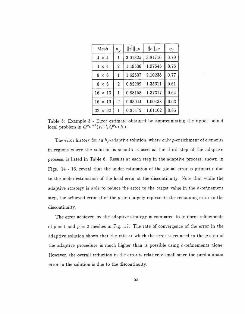
\Iesh p[" II·t· II.-tY IleliAu 1]['

"* x "* 1 3.01325 3.81716 0.79

"* x "* 2 1.49536 1.97645 0.76

8 x 8 1 1.62507 2.10238 0.77

8 x 8 2 0.82209 1.35611 0.61

16 x 16 1 0.88158 1.37317 0.64

16 x 16 'J 0,63044 1.00438 0.63

32 x 32 1 O.S;j4-;-2 1.01102 0.85

Table .S: Example 3 - Error estimate obtained by approximating the upper boundlocal problem in QP[,' ~I (1{) \ QP[,. (1\.'),

The error histon' for an hp-adaptiw solution. ,,,,here onl," p-enrichment of elements

in regions where the solution is smooth is used as the third step of the adaptive

process. is listed in Table 6. Results a.t each step in the a.daptive process. shown in

Figs. 14 - 16, reveal that the under-estimation of the global error is primarily due

to the under-estimation of the local error at the discontinuity. :-lote that while the

adaptive strat.egy is able to reduce the error to the target value in the h-refinement

step. the a.chieved error after the p step largely represents the remaining error in the

discontinui ty.

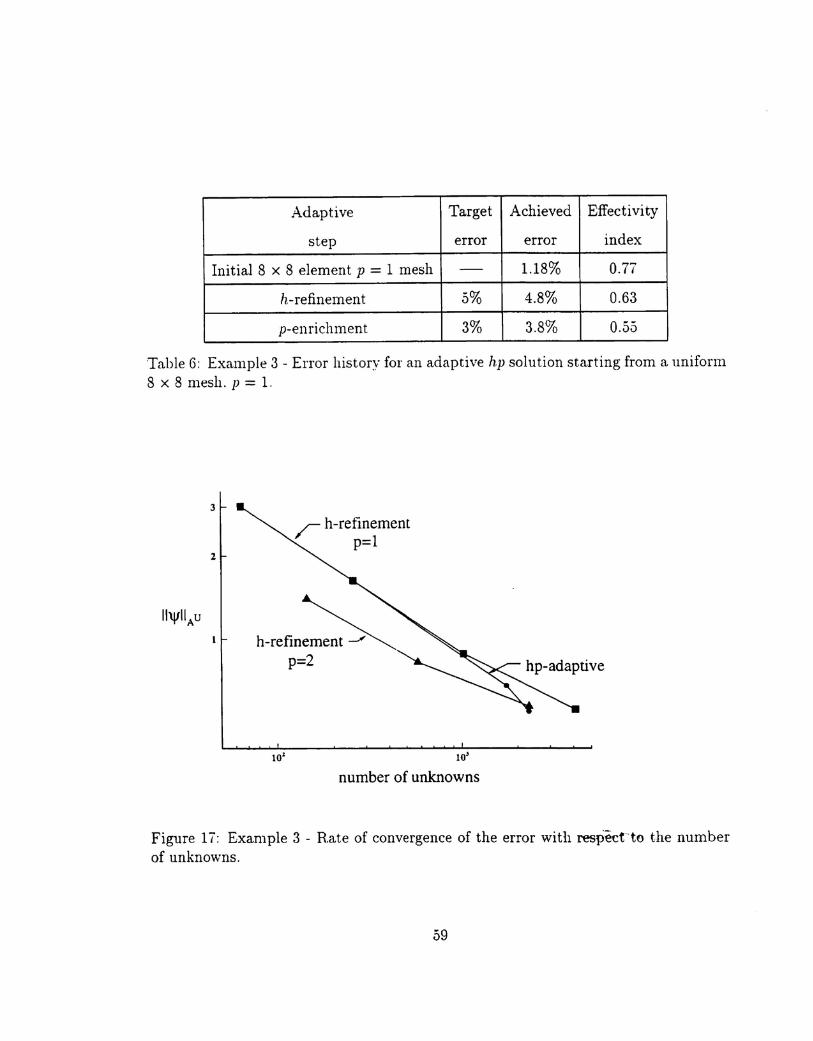
The error achieved by the ada.ptive strategy is compared to uniform refinements

of p = 1 and p = 2 meshes in Fig. 1-;-. The rate of convergence of the error in the

adaptive solution shows that the rate at which the error is reduced in the p-step of

the adaptive procedure is much higher than is possible using h.-refinements alone,

However, the overall reduction in the error is relatively small since the predominant

error in the solution is due to the discontinuity.

55

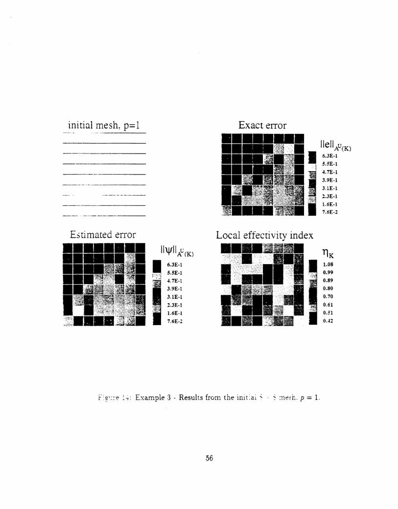
initial mesh~ p=l

Es rimmed error

1I\j111 AL' (K)

I,',,' 6.3E-l5.5E·lI':" ",

"," ~.7E·l

3.9E-l3.1E·12.3E-11.6E-17.6E-:

~.7E·13.9E·13.1E-12.3E-11.6E-1

7.6E·Z

11K1.08

0.990.890.800.100.610.51

0.42

f:g.l.::·e ~~: Example:3 - Results from the init:al";' ~ :ne5h. p = 1.

56

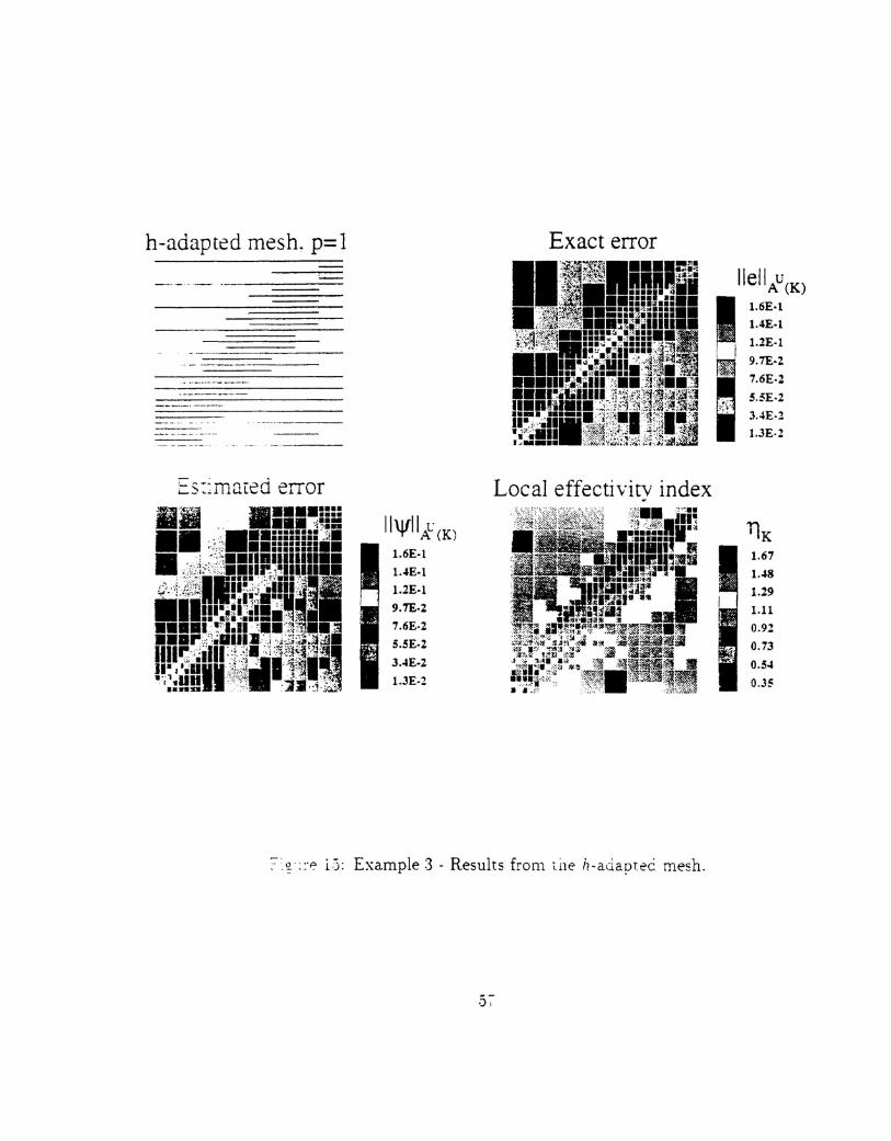
h-adapted mesh. p= 1'-- lIeIlAu(K)

!l.6E-l1.4E·l

,I l.2E-l

9,7E-2

I·7.6E·2

" S.5E·2,;;~ 3.4E-2

L3E·2

Es::mared errora'~ ••••• ::::-- ., ••• ':~:=•• " ••• :=:=:;=:J •. ~. ", ."",., 1•••

;':~':•• II•••IIIIII••

, ';-';,;:,t:~i;::~., •• 1r, i'!I, 11,1111.,""..'II···· '".,\...."';',":, ; "i:'~,' 11·" '0>11111<:"., ...'..", ......

~. ':,:",,;.1 .il~~••II!';' :'III·.~I·'~I.';,"'~1111..."•.....• ,.: •

••••• ,'~"I.II\ •• )F'?!•• ~••• r/\iUIII:.J.'.' ;,j;,n~;j~•1111" "'III" .". ····,"'··{,..,a'J.·'1_ ~-··;I _"'~,,.~.~,:~:.;....;:':~~J.....~ .,

JI. ';;~dll";L;j~I'':i~ll'"",•:;:~!i!!")''ij. :~j':1'%

11\Vlll(K)1.6E-l1.~E-l1.2E-l9.7E-27.6E-25.SE-23.~E-2L3E-2

Local effectivity index

1.671.48

1.291.11

0.920.730.540 ..35

,9,'::'-:' 1:"5:Example:3 - Results from tlle h-aciaptec: mesh .

.5-;-

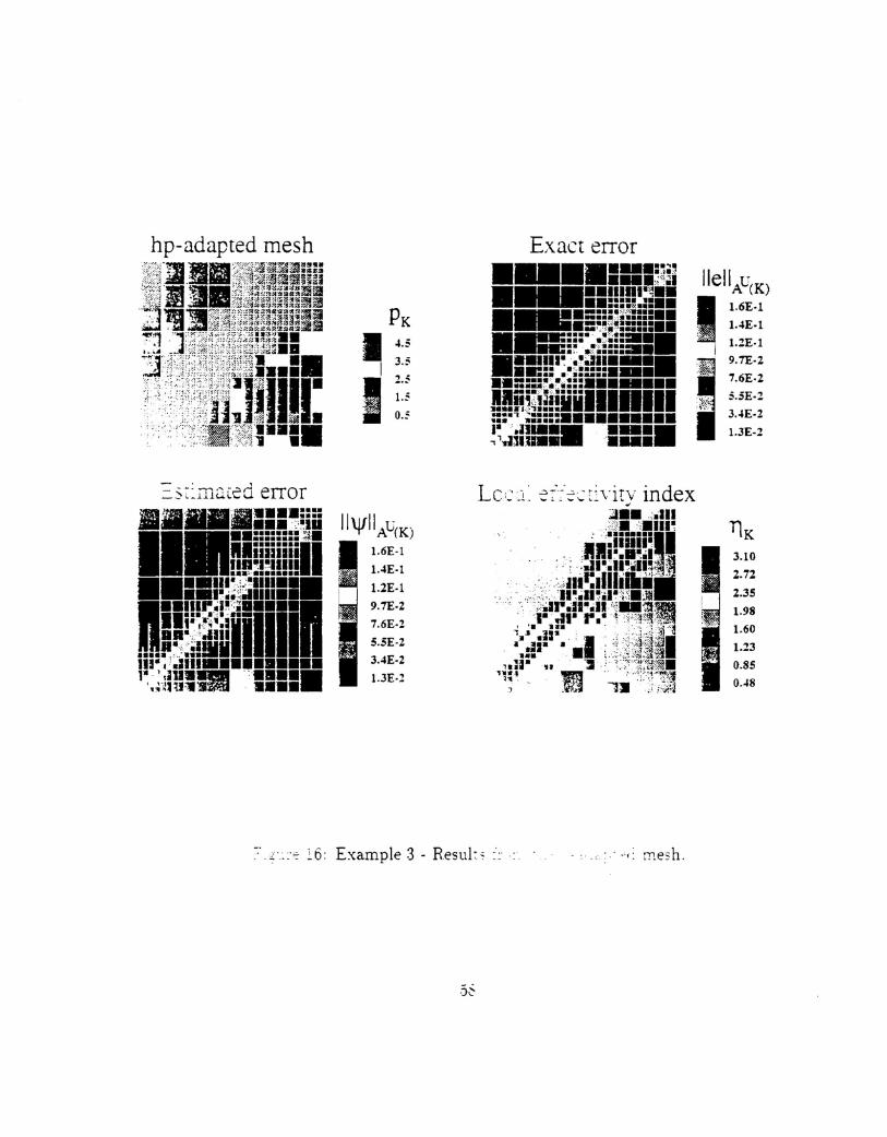
- -~.""",,,-~d error_.') L ....lllu..L"-

B!JI.8.' ;m•••• ::::__ •••• :'~Ia

IIII··::::===:~·IIliiiiiiiiIIn"'I~11111..., 11

•••• III·.:_:~IIII··11•• I~i.~"IIII••n··""I",I"""I"".. ",,'il,~':j·····n••

•••.• ',·:1-' •••

,. 1·~~~.1lin· .'.1111....!I~,;i_ldllm-. '.JlII ••••••••••1··',ID..... ':•••••

',~:~lU:w·S~ ••••

PKI ~.~

3.:-I ., ~

I',;:~. 0. .:'

11\VIIAlJ(K)1.6E-11.~E-11.2E-19.1£-27.6E-25.5£-23.4E-21.3E-2

Exact error-•...-.:,;'• _.,;·';~I•

_ •• lIlnl·~••..... ......... n ••••.-.-.,.,..,' " .- '.~ .II::~~~!=:::=:IIII._:::..~~::..•

••. .':;:11 ••••...",.....:..••• Inl~'.~dll._••.11::: .•~:::::._.•• :::-.:1"~~.:::••• _ •••.Jlii~7,'~ii..··11111111JI ••••• :.:. ., ••• !IIII:::., ~::::: .I·.n.... ._ .•.,'..J:'IIIIIIII',,_ •

3.10

2.722.351.981.60

1.230.850.~8

-"2'::"': 16: Example 3 - Resul:~ :':. :

Adaptive Target Achieved Effectivity

step error error index

Initial 8 x 8 element p = 1 mesh - 1.18% 0.77

h-refinement 5% 4.8% 0.63

p-enrichment 3% 3.8% 0.55

Table 6: Example 3 - Error history for an adaptive hp solution starting from a uniform8 x 8 mesh. p = 1,

3

2

10'

r h-refinementp=l

10'

number of unknowns

Figure 17: Example 3 - R.ate of convergence of the error with respect'to the numberof unknowns.

59

5 Concluding Remarks

The development of hp-version discontinuous Galerkin methods for hyperbolic conser-

vation laws is presented in this work. A priori error estimates are derived for a model

class of linear hyperbolic conservation laws. These estimates are obtained using a

new mesh-dependent norm that reflects the dependence of the approximate solution

on the local element size and the local order of approximation. The results generalize

and extend previous results on mesh-dependent norms to hp-version discontinuous

Galerkin methods.

A posteriori error estimates for the model problem are also developed. An exten-

sion of the element residual method to hvperbolic conservation la.ws result in estimates

which are proven to pro,-ide hounds on appropriate measures of the approxima.tion

error.

)l'umerical experiments verify the a priori estimates and demonstrate the effec-

tiveness of the a posteriori estimates in providing reliable estimates of the actual error

in the numerical solution. The numerical examples also illustrate the ability of an

hp-adaptive strategy to provide super-linear convergence rates with respect to the

number of unknowns in the problem, even for discontinuous solutions.

Among the major conclusions drawn from this work are the following:

1. The machinery of elliptic approximation theory can be extended to hp-finite

element approximations of hyperbolic equations using the not.ion of discontin-

uous Galerkin methods: this is made possible by the introduction of special

bilinear and linear forms which depend upon mesh parameters. the mesh size

h K of a element ]{ in the mesh and the spectral order P K of the shape functions

60

characterizing local approximations over the cell.

2. The use of the new mesh-dependent norms makes it possible to derive. for the

first time, a priori error estimates for non-uniform hp-approximations of linear

hyperbolic problems: these estimates are quasi-optimaL and the estimated rates

of convergence are fully confirmed by numerous numerical experiments.

3. Exponential and/or super-linear rates of convergence are obtained. even for

solutions with very 10\,,,' regularity: this justifies the llse of hp-methods and

demonstrates their superioritv over conventional methods for a model class of

problems,

.f, Rigorous Il po.·;fe1"iori eITor estimates are derived using a new version of the

element residual method: these estimates provide computa.ble measures of lora.!

(element,vise) error with remarkable accuracy in smooth regions and provide a.

reasonable basis for assessing solution quality and for adaptivity.

References

[1] Ainsworth. \1. and Oden . .1. T. ... A l'nified Approa.ch to A Posteriori Error

Estimation using Element Residual :vIethods." N~Lmerische Mathematik. Vol.

65, pp. 23-50, 1993.

[2] Ainsworth. \1. a.netOden. ,1. T. ..,A Procedure for A Posteriori Error Estimation

for h-p Finite Element \Iethods:' Computer lvfethods in Applied lvfechanics and

Engineering. Vol. 101. pp,73-96. 1992.

61

[3] Babuska, 1. and Suri. :'vI.."The hp- Version of the Finite Element :'vlethod with

Quasiuniform \Ieshes." Mathematical Modeling and Numerical Analysis. Vol.

21, pp. 199-238, 1987.

[4] Bank, R. E. and \Veiser. A., "Some A posteriori Error Estimates for Elliptic

Partial Differential Equations." Mathematics of Computations. Vol. 44. pp. 283-

301. 1985.

[;3] Bey, K, S..... \n hp-Adaptive Discontinuous Galerkin Met hod for Hyperbolic

Conservation La\vs," PhD Dissertation, The University of Texas a.t Austin.

Austin. TX, \Iav 1994.

[6] Biswas. R.. Devine. I~.. and Flaherty . .1,. '·Parallel. .\daptive Finite Element

\Iethou.s for Conservation La\vs." Department of Computer Science Technical

Report :-lo. 93-.5, R.enssela.er Polytechnic Institute, Troy, :-lew York, February:

1993.

[7] Ciarlet, P. G., The Finite Element Method for Elliptic Problems. :-lorth-

Holland. 1978,

[8] Cockburn, B., Hou. S., and Shu. C. \V., "The Runge-Kutta Local Projection

Discontinuous Galerkin ),ilethod for Conservation Laws IV: The Multidimen-

sional Case," Mathematics of Computations. Vol. 54. pp. 545-581, 1990.

[9] Cockburn. B, anu. Shu. C. \V .. "TVB Runge-Kutta Local Projection Discon-

tinuous Galerkin Finite Element :'vlethods for Conservation La'vs II: General

Framework," !vlathematics of Computations, Vol. 52, pp. 411-435, 1989,

62

[10] Demkowicz. L.. Devloo. P .. and Oden, .1. T .. "On an h.-type \'Iesh Refinement

Strategy based on \-Iinimization of Interpolation Errors,". Computer Methods

in Applied J..tfechanics and Engineering, Vol. 53, pp.6i-89. 1985.

[11] Dorr. \'1. R .. "The Approximation Theory for the p-Version of the Finite Ele-

ment Method," SIAM Journal of Numerical Analysis. Vol. 21, pp. 1180-1207,

1984.

[12] Johnson. c.. )laYert. C .. and Pitkaranta . .1 .. "Finite Element :\'Iethods for Linear

Hyperholic Prohlems." Computer lltfethods in Applied lvlechan:ics and Engineer-

ing. Vol. 45. pp. 28,)-312. 1984:.

[13] Johnson. C. and Pitkar;mta. L ...-\n Analysis of the Discontinuous Galerkin

\Iethod for a Scalar Hyperbolic Equation:' ]yfathematics of Comp1ltatioll~. Vol.

4:6, pp. 1-26. 1986.

[14] Lesaint, P. and Raviart, P.A., "On a Finite Element lvlethod for Solving the

:-leutron Transport Equation," Mathematical Aspects of Finite Elements

in Partial Differential Equations. Edited hy C. de Boor. Academic Press.

pp. 89-123. 1974:.

[15) Lohner, R., \-lorgan, K., and Zienkiewicz, O. C., .,Adaptive Grid Refinement

for the Compressible Euler Equations," Accuracy Estimates and Adaptive

Refinements in Finite Element Computations. Edited hy 1. Bahuska, O.

C. Zienkiewicz. J. Ga.go. and E. R.. de .-\, Oliviera. John \Viley and Sons, Ltd ..

Chichester. pp, 281-297, 1986,

63

[16] Oden,.T. T., Demkowicz. L .. Rachowicz, VV., and Westerman. T. A.. "Toward a

Universal II - P Adaptive Finite Element Strategy, Part 2: A Posteriori Error

Estimation," Computer Methods in Applied Mechanics and Engineering. Vol.

Ti, pp. 113-180. 1989.

[17] Oden . .T.T .. Demko"v-icz. L .. Strouboulis, T .. and Devloo. P ... ,Adaptive \Ieth-

ods for Problems in Solid and Fluid Mechanics," Accuracy Estimates and

Adaptive Refinements in Finite Element Computations. Edited b~.-1.

Bahuska. O. C. Zienkiewicz . .T. Gaga. and E, R. de A. Oliviera. John YViley and

Sons. Ltd .. Chichester. pp. 249-280. 1986.

[18] Oden . .T. T.. Patnt. A... and Feng, Y. S.. "An hp Adaptive Strategy". Adapti·ue.

Afultilevel. and Hierarch'leal Computational Strategies. A.. K. :'-Joor (fC'd.),_-\\ID-

Vol. 157, pp. 23-46. 1992.

[19] Peraire, J., Vahdati, \.J.. Morgan, K., and Zienkiewicz, O. C .. "Adaptive

Remeshing for Compressible Flow Computations:' Journal of Computational

Physics, VoL 72. pp. 449-466, 1987.

[20] Peraire, .T., \,Iorgan, I~.. aud Peiro . .T., "UnstructuredFinite Element \Iesh Gen-

eration and Adaptive Procedures for Computational Fluid Dynamics," AGARD

Conference Proceedings No. 464, pp. 18.1-18.12, 1990.

64