Harpur Hill, Buxton Derbyshire, SK17 9JN T: +44 (0)1298 218000 F: +44 (0)1298 218590 W: www.hsl.gov.uk

Assessment of Exposure to Light Mineral OilBased Metal Working Fluids

HSL/2000/22

Project Leader: Andrew Simpson

Author(s): Andrew Simpson BSc

Science Group: Environmental Measurement Group

© Crown copyright (2000)

Summary

Objectives

To investigate methods for measuring exposure to light mineral oil based metal working fluids.

Main Findings

The current HSE method cannot be used for measuring oil mist from metal working fluids based on light mineral oils. Standard filter sampling is unsuitable because volatile components in the oil collected on the filter may be lost by evaporation during sampling, resulting in an underestimation of the true mist concentration. During this work it was also found that;

w There can also be substantial losses during storage and in the equilibration period before gravimetric analysis.

w The loss of sample material can be reduced by refrigerating the filters during storage and reducing the equilibration time before gravimetric analysis.

w Immediate solvent desorption after sampling for subsequent analysis by Infra Red spectroscopy would also reduce losses.

Nevertheless evaporation during sampling is still likely to occur. Alternative methods were investigated for measuring total airborne oil (mist and vapour) and for measuring the vapour alone.

Total airborne oil can be sampled by a combination of a filter sampler (to collect mist) with a vapour sampler situated behind it (to sample original vapour and vaporised oil from the filter). The measurement of total oil should be more accurate than a measurement of only the mist as there should be little overall sample loss. It should be applicable to all mineral oil based metal working fluids. A number of types and combinations of samplers were considered, and the findings were;

w The conical inhalable sampler provides better splash protection for filters than the multi orifice sampler and is more compatible with the flow rates of commercially available sorbent tube vapour samplers.

w The preferred sorbent is XAD-2 because of its superior solvent desorption properties with perchloroethylene and, unlike charcoal, its capacity for sampling hydrocarbon vapour is not affected by humid atmospheres.

w In Germany the BIA (Berufsgenossenschaftliches Institut für Arbeitssicherheit) have a purpose designed system for sampling oil mist and vapour called the Gesamtsstaub-Gas-Probenahme (GGP) system. It has a conical inhalable sampler

combined with a large sorbent cartridge. The cartridge has a higher capacity for trapping analyte than commercial sorbent tubes but requires time consuming preparation involving much contact with perchloroethylene.

w The preferred sampling method is collection at 1 litre/min using a combination of the conical inhalable sampler with a 8 mm diameter XAD-2 sorbent tube, which can measure 8 hour samples between 0.1 and 33 mg/m³. An alternative arrangement, sampling at 2 litres/min using the more common multi orifice sampler connected to a 8 mm diameter charcoal tube is acceptable and can measure 0.1 to 83 mg/m³.

w Split flow pumped sorbent tubes were assessed as filter back up samplers but did not offer any advantages over full flow sorbent back up tubes for oil mist, being more complicated to set up and not performing as well.

w Diffusive Radiello samplers were assessed as filter back up samplers but were found to be not at all suitable due to the wide range in diffusive uptake rates of the various oil vapour components. Other diffusive samplers, such as Tenax ATD tubes may work as filter back up samplers but were not included in this work

Analytical methods for quantifying the sample material collected were also investigated;

w The preferred analytical method for both filters and sorbent is Infra Red spectroscopy using perchloroethylene as solvent. Gas chromatography can be used for sorbent samples and will provide some compositional information, separating components more or less by their boiling point, but it is not suitable for filter samples due to possible volatility problems with some potential components in metal working fluids.

w Any hydrocarbon solvent vapour sampled with the oil vapour will bias Infra Red measurements, and solvents with boiling points greater than ~170°C such as white spirit and kerosene will affect gas chromatographic analyses.

w Integral area or a combined peak absorbance of the methyl and methylene carbon - hydrogen bond stretches are better Infra Red measurements than the single methylene carbon - hydrogen bond stretch for quantifying oil.

Most of the methods considered for sampling total oil collected the inhalable fraction of the aerosol, ensuring that samples collected would be comparable with exposure limit values, and collected the mist and vapour separately. Consideration was also given to sampling both mist and vapour directly onto a pumped sorbent tube to see how well it compared, despite its poorer particle sampling characteristics;

w In limited circumstances pumped sorbent tubes could be used to indicate total airborne oil concentrations. Atmospheres would need to comprise of oil vapour concentrations considerably greater than the mist concentration. They are unlikely to be suitable for oils with viscosities much greater than 5 cSt at 40°C or flash points greater than 140°C.

w Samples were collected at 200 ml/min on 8 mm charcoal tubes and analysed by Infra Red spectroscopy. The substitution of XAD-2 for charcoal as sorbent would improve accuracy at low concentrations. Wider apertures and appropriate flow rates may improve their particle sampling characteristics.

Measurement of oil vapour was investigated as it was seen as a way of obtaining the true oil mist concentration from a total airborne oil concentration;

w Limited work suggested that oil vapour concentrations could be estimated in the presence of oil mist by standard diffusive sampling onto Tenax ATD tubes and analysis by thermal desorption - gas chromatography - flame ionisation detection. Tests found that although there was evidence that oil mist particles impacted, and oil vapour condensed on the internal walls, it may be possible to correct for the bias.

Two types of sampler were evaluated in field trials; the conical inhalable sampler with 8 mm XAD-2 sorbent back up tube, and lone pumped 8 mm charcoal tubes.

w The filter-XAD tube combination performed relatively well in the tests and generally gave higher results than the pumped charcoal tube.

w The presence of vapour from mineral spirits in the work place air invalidated some of the vapour samples. Whilst sampling for oil mist and vapour, it is important that the presence of interferents such as hydrocarbon solvent vapour are identified and avoided.

Main Recommendations

w Mineral oil mist and vapour should be sampled using pumped filter samples backed by sorbent tubes, the most appropriate combination being the conical inhalable sampler coupled with a 8 mm XAD-2 sorbent tube or alternatively the multi orifice sampler coupled to a 8 mm charcoal sorbent tube.

w Both filter and sorbent samples should be analysed by Fourier Transform Infra Red spectroscopy of the perchloroethylene extracts, measuring the combined peak absorbances of the methyl and methylene carbon - hydrogen bond stretches.

It would be useful to further characterise the method and its limitations by

w Determining the capacity of XAD-2 and charcoal sorbent tubes for oil vapour, and looking at the effect of high humidity on charcoal sorbent tube capacity.

w Looking at the effect of different base oils (e.g. naphthenic 60 solvent pale), additives (e.g. chlorinated paraffins), and mist types (i.e. condensation mists).

The applicability of the method could be further investigated by

w Looking at synthetic lubricants (e.g. poly-alpha-olefins and polybutenes) and mineral oil free non aqueous lubricants (e.g. esters such as rape seed oil).

w Further investigate the mist - vapour phase relationship, including filter sample losses, by sampling aerosols of oils with varying composition, and by investigating a wide range of potential additives.

Confidence in the quantification of diffusive samples of semi-volatile aliphatic hydrocarbons would be strengthened by

w Looking at naphthenic oils, non mineral oil lubricants and additives.

w Re-examining the problem of background subtraction for additional sampled oil, with the inclusion of work on condensation mists.

w Investigating the effect of multi component mixtures on uptake rates.

Further investigation of the effect of sampler design and flow rate on the particle sampling characteristics of sorbent tubes could provide simpler methods for sampling aerosols which contain significant quantities of volatile components, not just for a limited number of mineral oils but also for drilling muds and other semi-volatile compounds.

If measurement of total airborne oil is seen as an option to be explored further, it is recommended that HSE should aim to conduct a short survey to gain information on occupational exposure to oil mist and vapour from the light mineral oil metal working fluids not included in the recent Technical Development Survey.

Contents

1. INTRODUCTION . . . . . . . . . . . . . . . . . . . . . . . . . . . . . . . . . . . . . . . . . . . . . . . . . 1 2. EQUIPMENT . . . . . . . . . . . . . . . . . . . . . . . . . . . . . . . . . . . . . . . . . . . . . . . . . . . . 3 2.1. Samplers . . . . . . . . . . . . . . . . . . . . . . . . . . . . . . . . . . . . . . . . . . . . . . . . . . . . . 3 2.1.1. Reference Method - Conical Inhalable Sampler Connected to Three Impingers in Series . . . . . . . . . . . . . . . . . . . . . . . . . . . . . . . 4 2.1.2. Gesamtsstaub-Gas-Probenahme (GGP) Sampler . . . . . . . . . . . . . . . . . 5 2.1.3. Conical Inhalable Sampler Combined with Sorbent Tube . . . . . . . . . . . 5 2.1.4. Multi-Orifice Sampler Combined with Sorbent Tube . . . . . . . . . . . . . . . 5 2.1.5. Multi-Orifice Sampler Combined with Sorbent Tube in a Split Flow Configuration . . . . . . . . . . . . . . . . . . . . . . . . . . . . . . . . . . . . . . . . . . . . . 5 2.1.6. Conical Inhalable Sampler Combined with Radiello Tube Diffusive Sampler . . . . . . . . . . . . . . . . . . . . . . . . . . . . . . . . . . . . . . . . . . . . . . . . . . . 5 2.1.7. Pumped Charcoal Tube . . . . . . . . . . . . . . . . . . . . . . . . . . . . . . . . . . . . . . . 6 2.1.8. Diffusive Perkin Elmer ATD Tube . . . . . . . . . . . . . . . . . . . . . . . . . . . . . . . 6 2.2. Test Atmospheres . . . . . . . . . . . . . . . . . . . . . . . . . . . . . . . . . . . . . . . . . . . . . 6 2.2.1. Oil Mist Atmosphere . . . . . . . . . . . . . . . . . . . . . . . . . . . . . . . . . . . . . . . . . . . 6 2.2.2. Hydrocarbon Vapour Atmosphere . . . . . . . . . . . . . . . . . . . . . . . . . . . . . . . 6 3. METHOD DEVELOPMENT . . . . . . . . . . . . . . . . . . . . . . . . . . . . . . . . . . . . . . . 6 3.1. Investigation of Filter Sampling . . . . . . . . . . . . . . . . . . . . . . . . . . . . . . . . 6 3.1.1. Method . . . . . . . . . . . . . . . . . . . . . . . . . . . . . . . . . . . . . . . . . . . . . . . . . . . . . . 7 3.1.2. Results . . . . . . . . . . . . . . . . . . . . . . . . . . . . . . . . . . . . . . . . . . . . . . . . . . . . . . 8 3.1.3. Discussion . . . . . . . . . . . . . . . . . . . . . . . . . . . . . . . . . . . . . . . . . . . . . . . . . . . 8 3.1.4. Conclusion . . . . . . . . . . . . . . . . . . . . . . . . . . . . . . . . . . . . . . . . . . . . . . . . . . 12 3.2. Investigation of Analysis by Infra Red Spectroscopy . . . . . . . . . . . . 12 3.2.1. Method . . . . . . . . . . . . . . . . . . . . . . . . . . . . . . . . . . . . . . . . . . . . . . . . . . . . . 12 3.2.2. Results . . . . . . . . . . . . . . . . . . . . . . . . . . . . . . . . . . . . . . . . . . . . . . . . . . . . . 13 3.2.3. Discussion . . . . . . . . . . . . . . . . . . . . . . . . . . . . . . . . . . . . . . . . . . . . . . . . . . 13 3.2.4. Conclusion . . . . . . . . . . . . . . . . . . . . . . . . . . . . . . . . . . . . . . . . . . . . . . . . . . 19 3.3. Investigation of Analysis by Gas Chromatography -Flame Ionisation Detection . . . . . . . . . . . . . . . . . . . . . . . . . . . . . . . . . . . . . . . . 20 3.3.1. Method . . . . . . . . . . . . . . . . . . . . . . . . . . . . . . . . . . . . . . . . . . . . . . . . . . . . . 20 3.3.2. Results . . . . . . . . . . . . . . . . . . . . . . . . . . . . . . . . . . . . . . . . . . . . . . . . . . . . . 21 3.3.3. Discussion . . . . . . . . . . . . . . . . . . . . . . . . . . . . . . . . . . . . . . . . . . . . . . . . . . 21 3.3.4. Conclusion . . . . . . . . . . . . . . . . . . . . . . . . . . . . . . . . . . . . . . . . . . . . . . . . . . 27 3.4. Investigation of Diffusive Sampling . . . . . . . . . . . . . . . . . . . . . . . . . . . . 27 3.4.1. Method . . . . . . . . . . . . . . . . . . . . . . . . . . . . . . . . . . . . . . . . . . . . . . . . . . . . . 28 3.4.2. Results . . . . . . . . . . . . . . . . . . . . . . . . . . . . . . . . . . . . . . . . . . . . . . . . . . . . . 29 3.4.3. Discussion . . . . . . . . . . . . . . . . . . . . . . . . . . . . . . . . . . . . . . . . . . . . . . . . . . 29 3.4.4. Conclusion . . . . . . . . . . . . . . . . . . . . . . . . . . . . . . . . . . . . . . . . . . . . . . . . . . 34 3.5. Analysis of Factors Effecting Vapour Sampling on Sorbent Tubes . . . . . . . . . . . . . . . . . . . . . . . . . . . . . . . . . . . . . . . . . . . . . . . . . . . 35 3.5.1. Method . . . . . . . . . . . . . . . . . . . . . . . . . . . . . . . . . . . . . . . . . . . . . . . . . . . . . 35 3.5.2. Results . . . . . . . . . . . . . . . . . . . . . . . . . . . . . . . . . . . . . . . . . . . . . . . . . . . . . 36 3.5.3. Discussion . . . . . . . . . . . . . . . . . . . . . . . . . . . . . . . . . . . . . . . . . . . . . . . . . . 36 3.5.4. Conclusion . . . . . . . . . . . . . . . . . . . . . . . . . . . . . . . . . . . . . . . . . . . . . . . . . . 42

3.6. Investigation of Sampling Total Airborne Oil by Lone Pumped Sorbent Tubes . . . . . . . . . . . . . . . . . . . . . . . . . . . . . . . . . . . . . . . . . . . 44 3.6.1. Method . . . . . . . . . . . . . . . . . . . . . . . . . . . . . . . . . . . . . . . . . . . . . . . . . . . . . 44 3.6.2. Results . . . . . . . . . . . . . . . . . . . . . . . . . . . . . . . . . . . . . . . . . . . . . . . . . . . . . 45 3.6.3. Discussion . . . . . . . . . . . . . . . . . . . . . . . . . . . . . . . . . . . . . . . . . . . . . . . . . . 45 3.6.4. Conclusion . . . . . . . . . . . . . . . . . . . . . . . . . . . . . . . . . . . . . . . . . . . . . . . . . . 47 4. METHOD EVALUATION . . . . . . . . . . . . . . . . . . . . . . . . . . . . . . . . . . . . . . . . . 47 4.1. Laboratory Work . . . . . . . . . . . . . . . . . . . . . . . . . . . . . . . . . . . . . . . . . . . . . 47 4.1.1. Method . . . . . . . . . . . . . . . . . . . . . . . . . . . . . . . . . . . . . . . . . . . . . . . . . . . . . 48 4.1.2. Results . . . . . . . . . . . . . . . . . . . . . . . . . . . . . . . . . . . . . . . . . . . . . . . . . . . . . 48 4.1.3. Discussion . . . . . . . . . . . . . . . . . . . . . . . . . . . . . . . . . . . . . . . . . . . . . . . . . . 48 4.1.4. Conclusion . . . . . . . . . . . . . . . . . . . . . . . . . . . . . . . . . . . . . . . . . . . . . . . . . . 52 4.2. Method Selection . . . . . . . . . . . . . . . . . . . . . . . . . . . . . . . . . . . . . . . . . . . . . 53 4.3. Field Trial Visit 1 . . . . . . . . . . . . . . . . . . . . . . . . . . . . . . . . . . . . . . . . . . . . . 56 4.3.1. Sampling . . . . . . . . . . . . . . . . . . . . . . . . . . . . . . . . . . . . . . . . . . . . . . . . . . . 56 4.3.2. Analysis . . . . . . . . . . . . . . . . . . . . . . . . . . . . . . . . . . . . . . . . . . . . . . . . . . . . 59 4.3.3. Results . . . . . . . . . . . . . . . . . . . . . . . . . . . . . . . . . . . . . . . . . . . . . . . . . . . . . 59 4.3.4. Discussion . . . . . . . . . . . . . . . . . . . . . . . . . . . . . . . . . . . . . . . . . . . . . . . . . . 59 4.3.5. Conclusion . . . . . . . . . . . . . . . . . . . . . . . . . . . . . . . . . . . . . . . . . . . . . . . . . . 62 4.4. Field Trial Visit 2 . . . . . . . . . . . . . . . . . . . . . . . . . . . . . . . . . . . . . . . . . . . . . 62 4.4.1. Sampling . . . . . . . . . . . . . . . . . . . . . . . . . . . . . . . . . . . . . . . . . . . . . . . . . . . 62 4.4.2. Analysis . . . . . . . . . . . . . . . . . . . . . . . . . . . . . . . . . . . . . . . . . . . . . . . . . . . . 63 4.4.3. Results . . . . . . . . . . . . . . . . . . . . . . . . . . . . . . . . . . . . . . . . . . . . . . . . . . . . . 63 4.4.4. Discussion . . . . . . . . . . . . . . . . . . . . . . . . . . . . . . . . . . . . . . . . . . . . . . . . . . 63 4.4.5. Conclusion . . . . . . . . . . . . . . . . . . . . . . . . . . . . . . . . . . . . . . . . . . . . . . . . . . 65 5. REFERENCES . . . . . . . . . . . . . . . . . . . . . . . . . . . . . . . . . . . . . . . . . . . . . . . . . 66 6. APPENDIX A: INSTRUMENTAL CONDITIONS . . . . . . . . . . . . . . . . . . . . 69 7. APPENDIX B: ANALYTICAL RESULTS . . . . . . . . . . . . . . . . . . . . . . . . . . . 71 8. APPENDIX C: OIL MIST CHARACTERISTICS AND PROPERTIES . . . . . . . . . . . . . . . . . . . . . . . . . . . . . . . . . . . . . . . . . . . . . . . . . . . . 77 9. APPENDIX D: WIND TUNNEL RESULTS . . . . . . . . . . . . . . . . . . . . . . . . . 81 10. APPENDIX E: TEST SAMPLER FIGURES . . . . . . . . . . . . . . . . . . . . . . . 84

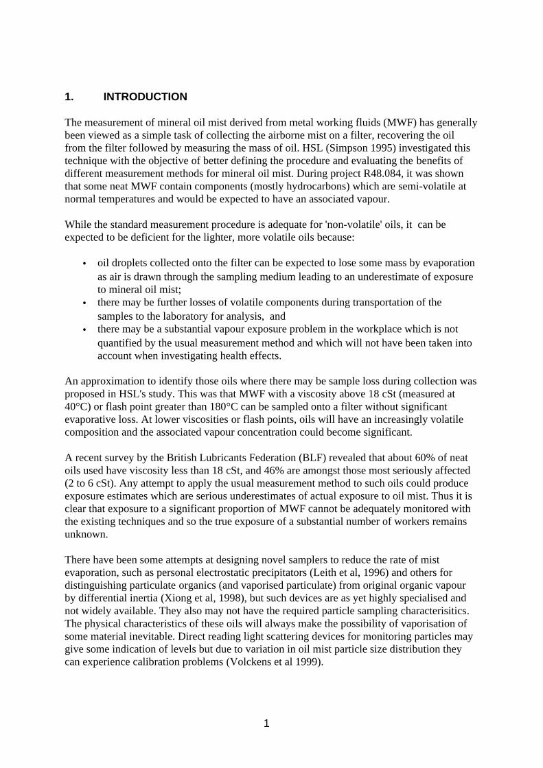
1. INTRODUCTION

The measurement of mineral oil mist derived from metal working fluids (MWF) has generally been viewed as a simple task of collecting the airborne mist on a filter, recovering the oil from the filter followed by measuring the mass of oil. HSL (Simpson 1995) investigated this technique with the objective of better defining the procedure and evaluating the benefits of different measurement methods for mineral oil mist. During project R48.084, it was shown that some neat MWF contain components (mostly hydrocarbons) which are semi-volatile at normal temperatures and would be expected to have an associated vapour.

While the standard measurement procedure is adequate for 'non-volatile' oils, it can be expected to be deficient for the lighter, more volatile oils because:

v oil droplets collected onto the filter can be expected to lose some mass by evaporation as air is drawn through the sampling medium leading to an underestimate of exposure to mineral oil mist;

v there may be further losses of volatile components during transportation of the samples to the laboratory for analysis, and

v there may be a substantial vapour exposure problem in the workplace which is not quantified by the usual measurement method and which will not have been taken into account when investigating health effects.

An approximation to identify those oils where there may be sample loss during collection was proposed in HSL's study. This was that MWF with a viscosity above 18 cSt (measured at 40°C) or flash point greater than 180°C can be sampled onto a filter without significant evaporative loss. At lower viscosities or flash points, oils will have an increasingly volatile composition and the associated vapour concentration could become significant.

A recent survey by the British Lubricants Federation (BLF) revealed that about 60% of neat oils used have viscosity less than 18 cSt, and 46% are amongst those most seriously affected (2 to 6 cSt). Any attempt to apply the usual measurement method to such oils could produce exposure estimates which are serious underestimates of actual exposure to oil mist. Thus it is clear that exposure to a significant proportion of MWF cannot be adequately monitored with the existing techniques and so the true exposure of a substantial number of workers remains unknown.

There have been some attempts at designing novel samplers to reduce the rate of mist evaporation, such as personal electrostatic precipitators (Leith et al, 1996) and others for distinguishing particulate organics (and vaporised particulate) from original organic vapour by differential inertia (Xiong et al, 1998), but such devices are as yet highly specialised and not widely available. They also may not have the required particle sampling characterisitics. The physical characteristics of these oils will always make the possibility of vaporisation of some material inevitable. Direct reading light scattering devices for monitoring particles may give some indication of levels but due to variation in oil mist particle size distribution they can experience calibration problems (Volckens et al 1999).

1

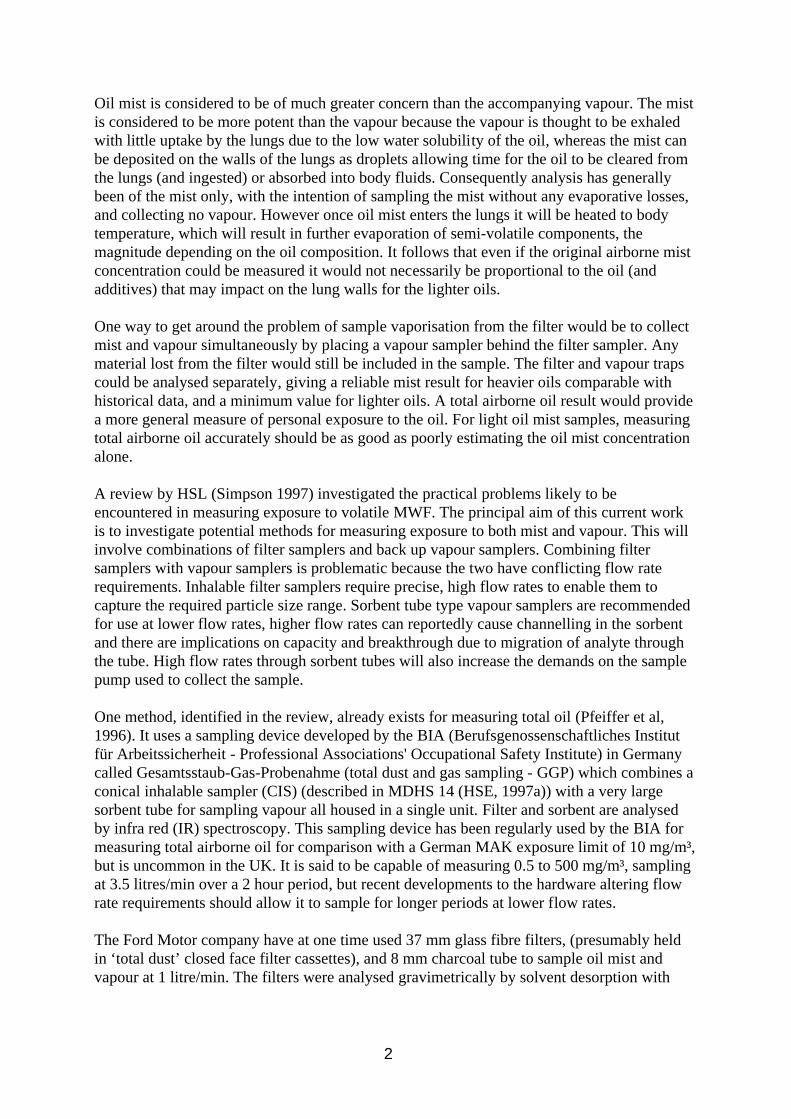
Oil mist is considered to be of much greater concern than the accompanying vapour. The mist is considered to be more potent than the vapour because the vapour is thought to be exhaled with little uptake by the lungs due to the low water solubility of the oil, whereas the mist can be deposited on the walls of the lungs as droplets allowing time for the oil to be cleared from the lungs (and ingested) or absorbed into body fluids. Consequently analysis has generally been of the mist only, with the intention of sampling the mist without any evaporative losses, and collecting no vapour. However once oil mist enters the lungs it will be heated to body temperature, which will result in further evaporation of semi-volatile components, the magnitude depending on the oil composition. It follows that even if the original airborne mist concentration could be measured it would not necessarily be proportional to the oil (and additives) that may impact on the lung walls for the lighter oils.

One way to get around the problem of sample vaporisation from the filter would be to collect mist and vapour simultaneously by placing a vapour sampler behind the filter sampler. Any material lost from the filter would still be included in the sample. The filter and vapour traps could be analysed separately, giving a reliable mist result for heavier oils comparable with historical data, and a minimum value for lighter oils. A total airborne oil result would provide a more general measure of personal exposure to the oil. For light oil mist samples, measuring total airborne oil accurately should be as good as poorly estimating the oil mist concentration alone.

A review by HSL (Simpson 1997) investigated the practical problems likely to be encountered in measuring exposure to volatile MWF. The principal aim of this current work is to investigate potential methods for measuring exposure to both mist and vapour. This will involve combinations of filter samplers and back up vapour samplers. Combining filter samplers with vapour samplers is problematic because the two have conflicting flow rate requirements. Inhalable filter samplers require precise, high flow rates to enable them to capture the required particle size range. Sorbent tube type vapour samplers are recommended for use at lower flow rates, higher flow rates can reportedly cause channelling in the sorbent and there are implications on capacity and breakthrough due to migration of analyte through the tube. High flow rates through sorbent tubes will also increase the demands on the sample pump used to collect the sample.

One method, identified in the review, already exists for measuring total oil (Pfeiffer et al, 1996). It uses a sampling device developed by the BIA (Berufsgenossenschaftliches Institut für Arbeitssicherheit - Professional Associations' Occupational Safety Institute) in Germany called Gesamtsstaub-Gas-Probenahme (total dust and gas sampling - GGP) which combines a conical inhalable sampler (CIS) (described in MDHS 14 (HSE, 1997a)) with a very large sorbent tube for sampling vapour all housed in a single unit. Filter and sorbent are analysed by infra red (IR) spectroscopy. This sampling device has been regularly used by the BIA for measuring total airborne oil for comparison with a German MAK exposure limit of 10 mg/m³, but is uncommon in the UK. It is said to be capable of measuring 0.5 to 500 mg/m³, sampling at 3.5 litres/min over a 2 hour period, but recent developments to the hardware altering flow rate requirements should allow it to sample for longer periods at lower flow rates.

The Ford Motor company have at one time used 37 mm glass fibre filters, (presumably held in ‘total dust’ closed face filter cassettes), and 8 mm charcoal tube to sample oil mist and vapour at 1 litre/min. The filters were analysed gravimetrically by solvent desorption with

2

trichloroethylene or perchloroethylene, the sorbent by solvent desorption with carbon disulphide and analysis by gas chromatography (GC). The sampler would not have collected the inhalable fraction required for comparison with UK limit values, and it is uncertain whether the procedure took precautions to minimise filter sample losses during storage and equilibration.

An alternative to the GGP sampler using more familiar and more common inhalable filter samplers (such as the Institute of Occupational Medicine (IOM) sampler or the multi-orifice sampler (MOS)) would be to combine them in series with commercially available sorbent tubes. Such combinations need to be tested to see quite what restrictions the problems mentioned will have on application and performance. One way to overcome these problems would be to reduce the flow rate through a sorbent tube whilst maintaining the required high flow rate through the filter sampler by splitting the air flow, so that only a portion of the air sampled through the filter also goes through the sorbent tube. Another strategy would be to use a diffusive sampler behind the filter sampler to sample the vapour. A diffusive sampler should present no problems associated with pumped sorbent tubes, but will have problems of its own, namely sensitivity and knowledge of the uptake rates of the analytes involved. An alternative to combining filter and vapour samplers may be to sample both using just a pumped sorbent tube, however such a method would not necessarily sample the inhalable fraction of the mist usually required for comparison with limit values.

If the vapour concentration could be accurately determined, it should be possible to calculate a mist concentration from the total oil concentration. Pumped sampling methods will sample some mist, however diffusive sampling methods may be unaffected by the presence of mist particles and offer a way of measuring the vapour only concentration.

Analytical methods for oil mist on filters are well established, but as yet no work has been done on the effect of potential evaporative losses from filters of light mineral oil mist samples during storage. The mist (and vapour) from these types of oils will differ in composition from the bulk oil and this may have implications on calibration of IR spectroscopic methods. Apart from IR spectroscopy, GC appears to be the only widely applicable alternative method for measuring the vapour, however sensitivity and choice of calibration material may cause problems.

Once estasblished, suitable sampling and analytical methods for measuring exposure to volatile mineral oil based MWF are to be evaluated by initially sampling artificial aerosols of a commercial MWF in the laboratory, and then by use in the field.

2. EQUIPMENT

2.1. Samplers

Most of the sampling devices tested were combinations of filter samplers to trap the mist connected in series with some type of vapour trap behind. The filter samplers used were ones which collect the inhalable fraction of the aerosol, ensuring that the samples collected will be comparable with exposure limit values. Such samplers are described in MDHS 14 (HSE 1997a), and include the IOM, MOS and CIS samplers. Table 1 illustrates some of the samplers characteristics.

3

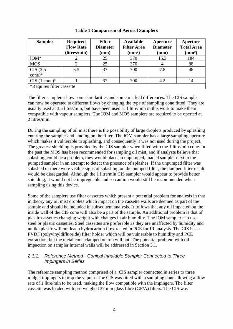
Table 1 Comparison of Aerosol Samplers

Sampler Required Flow Rate (litres/min)

Filter Diameter

(mm)

Available Filter Area

(mm²)

Aperture Diameter

(mm)

Aperture Total Area

(mm²) IOM* 2 25 370 15.3 184 MOS 2 25 370 4 88 CIS (3.5 cone)*

3.5 37 700 7.8 48

CIS (1 cone)* 1 37 700 4.2 14 *Requires filter cassette

The filter samplers show some similarities and some marked differences. The CIS sampler can now be operated at different flows by changing the type of sampling cone fitted. They are usually used at 3.5 litres/min, but have been used at 1 litre/min in this work to make them compatible with vapour samplers. The IOM and MOS samplers are required to be operted at 2 litres/min.

During the sampling of oil mist there is the possibility of large droplets produced by splashing entering the sampler and landing on the filter. The IOM sampler has a large sampling aperture which makes it vulnerable to splashing, and consequently it was not used during the project. The greatest shielding is provided by the CIS sampler when fitted with the 1 litre/min cone. In the past the MOS has been recommended for sampling oil mist, and if analysts believe that splashing could be a problem, they would place an unpumped, loaded sampler next to the pumped sampler in an attempt to detect the presence of splashes. If the unpumped filter was splashed or there were visible signs of splashing on the pumped filter, the pumped filter result would be disregarded. Although the 1 litre/min CIS sampler would appear to provide better shielding, it would not be impregnable and so caution would still be recommended when sampling using this device.

Some of the samplers use filter cassettes which present a potential problem for analysis in that in theory any oil mist droplets which impact on the cassette walls are deemed as part of the sample and should be included in subsequent analysis. It follows that any oil impacted on the inside wall of the CIS cone will also be a part of the sample. An additional problem is that of plastic cassettes changing weight with changes in air humidity. The IOM sampler can use steel or plastic cassettes. Steel cassettes are preferable as they are unaffected by humidity and unlike plastic will not leach hydrocarbon if extracted in PCE for IR analysis. The CIS has a PVDF (polyvinyldifluoride) filter holder which will be vulnerable to humidity and PCE extraction, but the metal cone clamped on top will not. The potential problem with oil impaction on sampler internal walls will be addressed in Section 3.1.

2.1.1. Reference Method - Conical Inhalable Sampler Connected to Three Impingers in Series

The reference sampling method comprised of a CIS sampler connected in series to three midget impingers to trap the vapour. The CIS was fitted with a sampling cone allowing a flow rate of 1 litre/min to be used, making the flow compatible with the impingers. The filter cassette was loaded with pre-weighed 37 mm glass fibre (GF/A) filters. The CIS was

4

connected to the impingers via inert glass or teflon tubing. The impingers were filled with 20 ml HPLC grade perchloroethylene (PCE), a solvent suitable for IR analysis for hydrocarbons, and also for use within impingers.

2.1.2. Gesamtsstaub-Gas-Probenahme (GGP) Sampler

This is a commercially available sampler which comprises of a CIS filter sampler with a built in cartridge, packed by the user with an appropriate sorbent (e.g. Figure E1, Appendix E). The filter cassette was loaded with pre-weighed 37 mm GF/A filters. The cartridge was loaded with 3g of pre-treated XAD-2 sorbent. The samplers were fitted with cones allowing a flow rate of 1 litre/min.

2.1.3. Conical Inhalable Sampler Combined with Sorbent Tube

A CIS sampler loaded with a pre-weighed 37 mm GF/A filter was combined via a short length of plastic tube to an 8 mm diameter sorbent back up tube (e.g. Figure E2, Appendix E). Both charcoal and XAD-2 sorbent tubes were used in tests as back up tubes. The sorbent tubes comprise a 400 mg sampling layer and a 200 mg back up layer to check for breakthrough. The 8 mm diameter tubes have a recommended maximum flow rate of 1 litre/min, compatible with the CIS samplers when fitted with the 1 litre/min cones.

2.1.4. Multi-Orifice Sampler Combined with Sorbent Tube

A MOS sampler loaded with a pre-weighed 25 mm GF/A filter was combined via a short length of plastic tube to an 8 mm diameter charcoal sorbent back up tube. The MOS samplers were operated at their required flow rate of 2 litres/min in order to test the perfomance of the sorbent tubes at above their recommended maximum flow rate.

2.1.5. Multi-Orifice Sampler Combined with Sorbent Tube in a Split Flow Configuration

A system was constructed whereby a MOS sampler loaded with a pre-weighed 25 mm GF/A filter was connected to a sorbent tube holder which allowed 0.4 litres/min through a 6 mm diameter charcoal tube and the remaining 1.6 litres/min through a by-pass tube (e.g. Figure E3, Appendix E). One critical orifice was used to set the charcoal tube flow, while a second critical orifice (fully open) on the by-pass side was needed to create sufficient back pressure for the first to work, allowing the whole to be operated by a single sampling pump. Total flow (sorbent tube and by-pass tube) was set at 2 litres/min via the pump. The CIS sampler was not used to test this configuration because it could already be combined with sorbent tubes at recommended flow rates. The 6 mm charcoal tubes contain 100 and 50 mg layers of sorbent and have a maximum recommended flow rate of 0.5 litres/min.

2.1.6. Conical Inhalable Sampler Combined with Radiello Tube Diffusive Sampler

A CIS sampler was used to collect the mist (at 1 litre/min), and the vapour passing through the filter was directed past a Radiello diffusive sampler held in a canister (manufactured at HSL), and loaded with ~210 mg of activated charcoal in a 3.9 mm diameter cartridge (e.g. Figure E4, Appendix E). The Radiello tube was chosen as the diffusive sampler because

5

its higher mass uptake rates would be more suited to sampling low levels of hydrocarbon vapour. It would also be possible to use the Radiello tube in combination with the MOS sampling at 2 litres/min, CIS samplers were used in order to make more appropriate comparisons with the reference method.

2.1.7. Pumped Charcoal Tube

Pumped charcoal tubes, widely used for sampling solvent vapours were used to sample both mist and vapour. The tubes used were either the standard 6 mm diameter tube or the larger 8 mm diameter tubes. Two sizes of tube were used to see if any effects on the sampling efficiency of the mist particles could be detected.

2.1.8. Diffusive Perkin Elmer ATD Tube

Standard Perkin Elmer ATD tube packed with Tenax TA sorbent was used to try and sample the vapour only, without any influence from the mist particles.

2.2. Test Atmospheres

2.2.1. Oil Mist Atmosphere

Atmospheres of oil mist were generated in a small wind tunnel. Air was driven down a tunnel of cross sectional area 0.5 m² at 0.8 m/s (24 m³/min). An aerosol of a relatively volatile oil based MWF was produced by the spinning disc method. Oil was dripped onto the centre of a disc spinning at approximately 1800 rps, which atomised the oil into an aerosol. The mist drifted 3.3 m down the tunnel to the samplers in ~4 seconds, during which a portion of the oil evaporated from the particles to produce an accompanying vapour. The samplers were placed centrally in the tunnel in a 3 x 3 array facing the oncoming mist. The particle size distribution produced was examined using a Climet Model CI208 Particle analyser. In terms of numbers, most of the particles produced were between 1 and 3 µm in diameter, but in terms of mass, the diameter range 3 to 5 µm was most abundant (Table D1 in Appendix D).

2.2.2. Hydrocarbon Vapour Atmosphere

Hydrocarbon vapour atmospheres were created in the standard atmosphere test rig described in project S20 065 96, (Unwin et al 1997). Samplers were exposed to the vapour inside a 14 litre temperature controlled glass chamber. The test air mixture was fed into the chamber at 20 litres/min, at a controlled temperature and humidity. A constant concentration of the analyte vapour was introduced into the air stream via a syringe injection system (HSE, 1990). Air temperature and relative humidity (RH) were monitored via a Vaisala HMI32 temperature-relative humidity meter.

3. METHOD DEVELOPMENT

3.1. Investigation of Filter Sampling

There are several problems associated with filter sampling of oil mist, principally vaporisation of components from trapped mist particles during sampling and vaporisation of material

6

during storage. Some of the samplers use filter cassettes, and any aerosol which impacts on the internal walls of the cassette is deemed a part of the sample. The CIS sampler comprises a filter held in a PVDF filter holder upon which is clamped a sampling cone, and in theory any oil impacted on the inside walls of the cone and the holder would constitute part of the sample which would not be accounted for if subsequent analysis was of the filter only. This complicates solvent extraction of the samples, not least because the PCE used in the IR analysis will extract hydrocarbon material from many polymers.

3.1.1. Method

Evaporative Losses During Sampling

In the preceding work (Simpson, 1995) the potential for sample loss by evaporation was estimated by pipetting oil onto filters and aspirating them with clean air in the same manner as occurs during sampling. The filters were then reweighed periodically to measure the rate of loss. The experiment gave an indication of the problem, but the method used to spike the filters was not ideal, giving a sample identical in composition to the bulk oil and having a much lower surface area. During work setting up the wind tunnel the opportunity was taken to repeat this work for the oil using more realistic samples. Nine MOS loaded with preweighed 25 mm GF/A filters were used to sample oil mist in the wind tunnel (described in Section 2.2.1, and using the conditions listed in Table A1 in Appendix A) for 105 minutes at 2 litres/min. After sampling the filters were immediately reweighed to determine the amount of oil loaded onto the filter. The filters were reloaded into the samplers and were then set to sample clean laboratory air at 2 litres/min for 4 hours, stopping and reweighing the filters after ½, 1, 2, 3 and 4 hours. Two reference samples (see Section 2.1.1) were taken during the first part of the experiment to measure the aerosol / vapour relationship. Three blank filters were run in parallel during the second section of the experiment to correct for effects of any airborne dust or humidity changes.

Filter Storage Trials

To investigate losses during storage, oil mist samples were collected on preweighed GF/A filters, re-weighed immediately after sampling and then again after a period of time in storage. Three situations were investigated; leaving the filters overnight in open sample tins at room temperature before reweighing (as recommended in MDHS 14 (HSE, 1997a), the general method for collecting particulate samples on filters), storing in sealed sample tins at room temperature and reweighing after 1, and 7 days, and storing in sealed tins in a refrigerator and reweighing after 1 and 7 days. This work was initially done with 25 mm filters collected in multi-orifice samplers at 2 litres/min during work setting up the tunnel. It was repeated during testing of the vapour samplers using 37 mm filters in CIS samplers operating at 1 litre/min. Filters collected in CIS filter holders were weighed separately from the holder due to errors introduced by weight changes to the holder caused by air humidity.

Sample Loss by Mist Impaction on Sampler Internal Walls

The problem of oil impaction on internal walls of the CIS samplers was investigated by analysis for oil after they had been used for sampling oil mist in the wind tunnel for 4 hours. The filter holder and cone were cleaned before sampling. After sampling the inside surface of

7

the filter holder was wiped with a glass fibre filter which was then extracted in 10 ml PCE for 1 hour. The inside surface of the cone was extracted initially by rinsing with 10 ml PCE, latterly by wiping with a glass fibre filter as per the filter holders. The PCE extracts were then analysed by FTIR using the method described in Table A2 in Appendix A.

3.1.2. Results

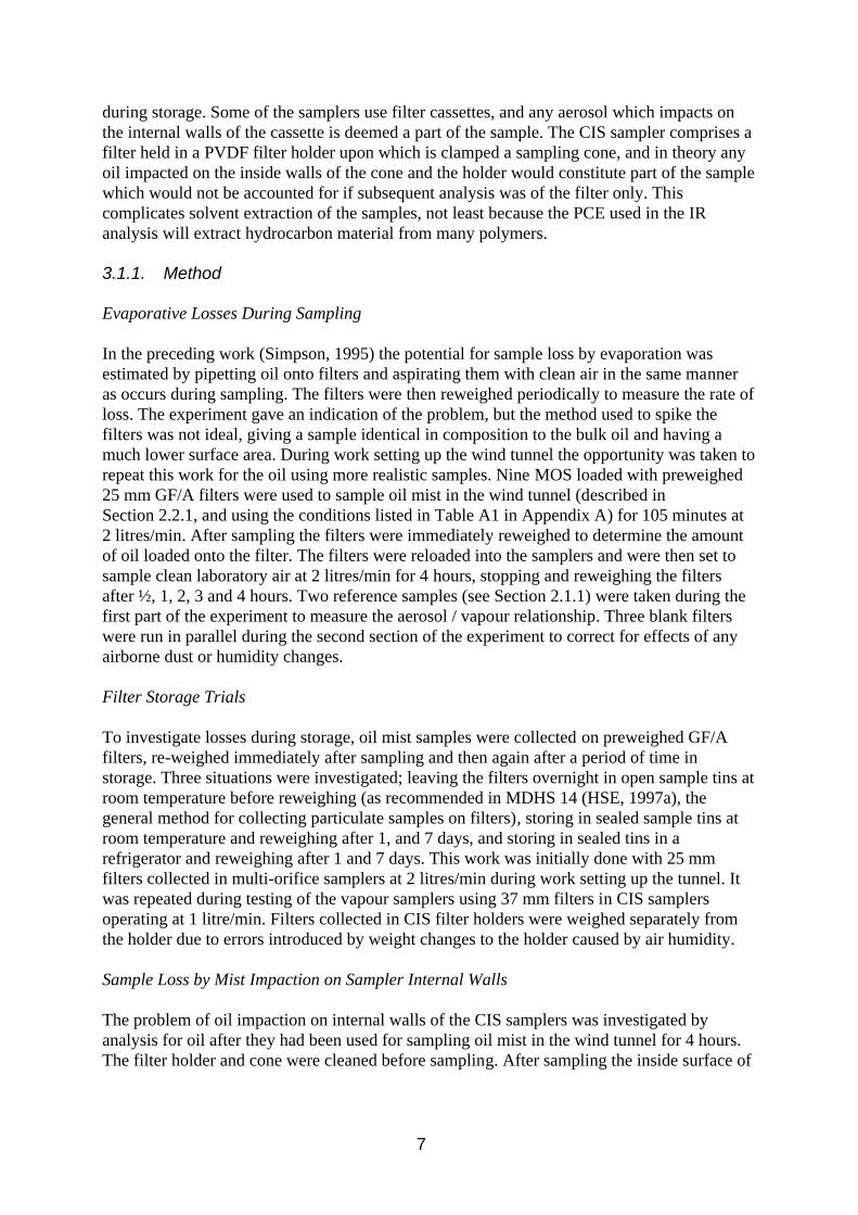
The results of the evaporative sample loss experiment are shown in Figure 1 and Table 2. The mean total inhalable particulate (TIP) concentration of the nine MOS samplers was 7.8 mg/m3. The reference method mean mist concentration was 7.9 mg/m3, and the mean vapour concentration was 15.3 mg/m3.

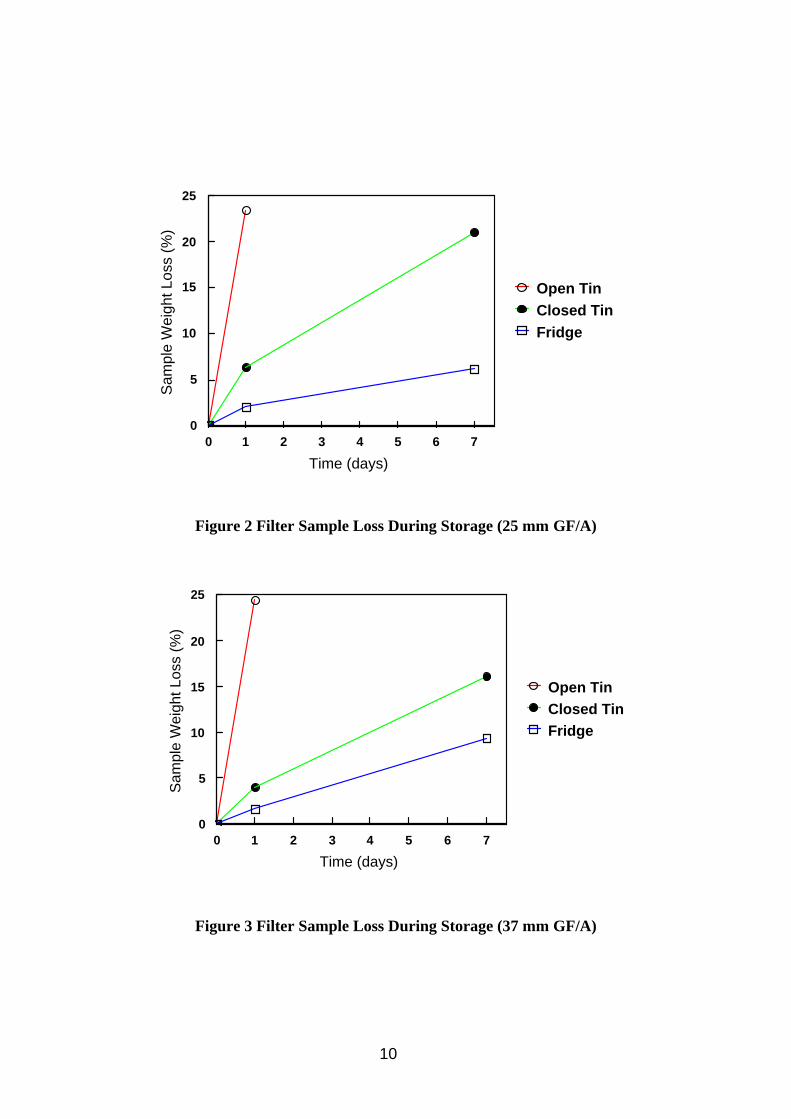
The results of the filter sample storage trials are presented in Table 3 and Figures 2 and 3.

The results of the work on oil impaction on sampler internal walls are presented in Table 4.

3.1.3. Discussion

Evaporative Losses During Sampling

Material was lost from the filter throughout the 4 hours. The rate of loss slowed down over time but was still quite noticeable. It can be estimated that the loss of sample rose above the 5% level in the first five or ten minutes. It is clear that filter samples taken of mist from this MWF will not be quantitative, however it would be desirable to maintain filter sampling using inhalable samplers so that a standardised fraction of the aerosol, linked to health based criteria can be collected.

70

60

50

40

30

20

10

0

Sam

ple

Wei

ght L

oss

(%)

0 60 120 180 240

Time (mins)

Figure 1 Rate of Loss of Material from the Sample Filter During Aspiration with Clean Air

8

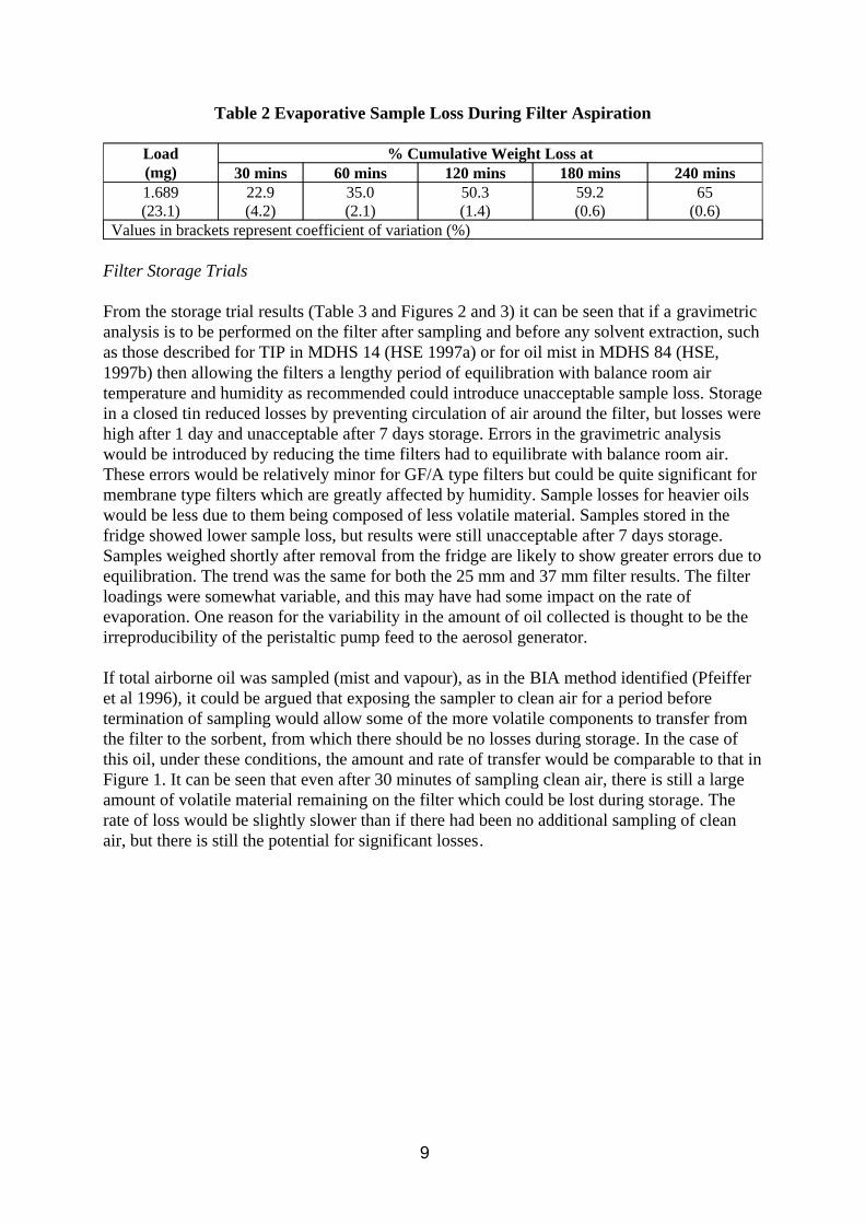
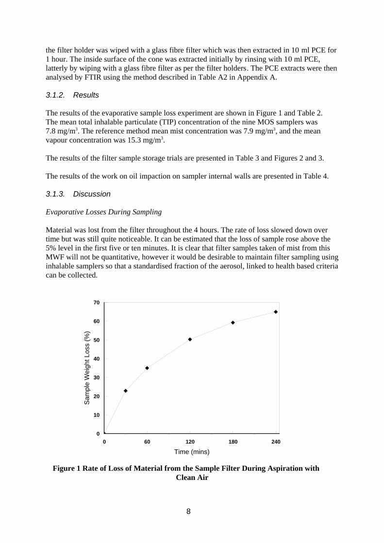
Table 2 Evaporative Sample Loss During Filter Aspiration

Load (mg)

% Cumulative Weight Loss at 30 mins 60 mins 120 mins 180 mins 240 mins

1.689 (23.1)

22.9 (4.2)

35.0 (2.1)

50.3 (1.4)

59.2 (0.6)

65 (0.6)

Values in brackets represent coefficient of variation (%)

Filter Storage Trials

From the storage trial results (Table 3 and Figures 2 and 3) it can be seen that if a gravimetric analysis is to be performed on the filter after sampling and before any solvent extraction, such as those described for TIP in MDHS 14 (HSE 1997a) or for oil mist in MDHS 84 (HSE, 1997b) then allowing the filters a lengthy period of equilibration with balance room air temperature and humidity as recommended could introduce unacceptable sample loss. Storage in a closed tin reduced losses by preventing circulation of air around the filter, but losses were high after 1 day and unacceptable after 7 days storage. Errors in the gravimetric analysis would be introduced by reducing the time filters had to equilibrate with balance room air. These errors would be relatively minor for GF/A type filters but could be quite significant for membrane type filters which are greatly affected by humidity. Sample losses for heavier oils would be less due to them being composed of less volatile material. Samples stored in the fridge showed lower sample loss, but results were still unacceptable after 7 days storage. Samples weighed shortly after removal from the fridge are likely to show greater errors due to equilibration. The trend was the same for both the 25 mm and 37 mm filter results. The filter loadings were somewhat variable, and this may have had some impact on the rate of evaporation. One reason for the variability in the amount of oil collected is thought to be the irreproducibility of the peristaltic pump feed to the aerosol generator.

If total airborne oil was sampled (mist and vapour), as in the BIA method identified (Pfeiffer et al 1996), it could be argued that exposing the sampler to clean air for a period before termination of sampling would allow some of the more volatile components to transfer from the filter to the sorbent, from which there should be no losses during storage. In the case of this oil, under these conditions, the amount and rate of transfer would be comparable to that in Figure 1. It can be seen that even after 30 minutes of sampling clean air, there is still a large amount of volatile material remaining on the filter which could be lost during storage. The rate of loss would be slightly slower than if there had been no additional sampling of clean air, but there is still the potential for significant losses.

9

0

5

10

15

20

25

Sam

ple

Wei

ght L

oss

(%)

Open Tin Closed Tin Fridge

0 1 2 3 4 5 6 7

Time (days)

Figure 2 Filter Sample Loss During Storage (25 mm GF/A)

25

Sam

ple

Wei

ght L

oss

(%)

20

15

10

5

0 0 1 2 3 4 5 6 7

Time (days)

Open Tin Closed Tin Fridge

Figure 3 Filter Sample Loss During Storage (37 mm GF/A)

10

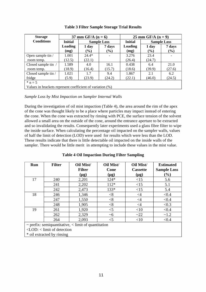
Table 3 Filter Sample Storage Trial Results

Storage Conditions

37 mm GF/A (n = 6) 25 mm GF/A (n = 9) Initial

Loading (mg)

Sample Loss Initial Loading

(mg)

Sample Loss 1 day (%)

7 days (%)

1 day (%)

7 days (%)

Open sample tin / 1.001 24.4* - 3.276 23.4 -room temp. (12.5) (22.1) (26.4) (24.7)

Closed sample tin / 1.589 4.0 16.1 0.438 6.4 21.0 room temp. (18.9) (16.4) (15.7) (18.6) (39.9) (27.6)

Closed sample tin / 1.021 1.7 9.4 1.867 2.1 6.2 fridge (5.9) (23.9) (24.2) (22.1) (46.0) (24.5) * n = 5 Values in brackets represent coefficient of variation (%)

Sample Loss by Mist Impaction on Sampler Internal Walls

During the investigation of oil mist impaction (Table 4), the area around the rim of the apex of the cone was thought likely to be a place where particles may impact instead of entering the cone. When the cone was extracted by rinsing with PCE, the surface tension of the solvent allowed a small area on the outside of the cone, around the entrance aperture to be extracted and so invalidating the results. Consequently later experiments used a glass fibre filter to wipe the inside surface. When calculating the percentage oil impacted on the sampler walls, values of half the limit of detection (LOD) were used for results which were less than the LOD. These results indicate that there is little detectable oil impacted on the inside walls of the sampler. There would be little merit in attempting to include these values in the mist value.

Table 4 Oil Impaction During Filter Sampling

Run Filter Oil Mist/ Filter (µg)

Oil Mist/ Cone (µg)

Oil Mist/ Cassette

(µg)

Estimated Sample Loss

(%) 17 240 2,201 124* <15 5.6

241 2,202 112* <15 5.1 242 2,473 133* <15 5.4

18 246 1,346 <8 <4 <0.4 247 1,550 <8 <4 <0.4 248 1,905 <8 <4 <0.3

19 261 1,920 <5 <10 <0.4 262 2,329 ~6 ~22 ~1.2 264 2,093 <5 <10 <0.4

~ prefix: semiquantitative, < limit of quantitation <LOD: < limit of detection * oil extracted by rinsing

11

3.1.4. Conclusion

w The amount of oil quantified on the filter represents a minimum estimate for the mist captured, as volatile components will evaporate from the filter. The degree of sample loss is dependant on the type of MWF sampled.

w Significant amounts of sample can be lost after sampling during storage. For oils such as that tested here it is recommended that analysis or solvent extraction for later analysis should take place within a day of sampling if not immediately after sampling. Samples in transit or storage should ideally be kept cold.

w Gravimetric analyses of filters recommend allowing the filters to equilibrate with balance room temperature and humidity overnight before analysis, however for oil mist samples a substantial portion may be lost by evaporation, and so it is recommended that the equilibration time is reduced and that glass fibre filters are more appropriate than membrane filters.

w Little of the total sample is impacted on the walls of the CIS sampler, and analysis of the filter alone will be sufficient.

3.2. Investigation of Analysis by Infra Red Spectroscopy

Infra red (IR) was considered the most appropriate spectroscopic method due to its applicability to all mineral oils, and its having a narrower range of sensitivities to different oils (however MWF contain both mineral oils and additives). Fourier Transform Infra Red (FTIR) was used for the analysis to improve accuracy and aid data handling. In the BIA method (Pfeiffer et al, 1996) the integral area of the carbon hydrogen bond stretch bands is measured, however NIOSH (NIOSH, 1994a) measure the largest peak absorbance (the methylene carbon hydrogen bond stretch). In this work the most appropriate criteria for measuring the oil was investigated by assessing a range of neat base oils and MWF, and by analysis of samples collected in the wind tunnel. Perchloroethylene (PCE) was used as the solvent for the work, used successfully in the previous work, it was chosen then because it is less toxic than carbon tetrachloride and likely to be cheaper and more widely available than the CFC 1,1,2 trichlorotrifluoroethane. It is also more suitable for use in the impingers of the reference method because of its higher boiling point. IR can be used to measure vapour and mist samples.

3.2.1. Method

The sensitivity range of a number of base oils and hydrocarbon solvents were investigated by analysing 100 µg/ml solutions of bulk fluid in PCE and analysing them using the conditions listed in Table A2 in Appendix A. The range of sensitivities of MWF was investigated by re-analysing spectra collected during previous work on MWF (Simpson, 1995)). The baseline corrected peak absorbances at 2957 cm-1 (methyl C-H stretch) and 2926 cm-1 (methylene C-H stretch), and the integral areas were measured and corrected for solution concentration differences by calculating response factors (Rf). A combined measurement of the sum of the absorptions at 2957 and 2926 cm-1 was also calculated. Extinction coefficients were not calculated due to the lack of an analyte molecular weight value.

12

Filter and impinger samples taken of aerosols generated in the wind tunnel were analysed by FTIR. The filters were weighed before and after sampling to determine the TIP (MDHS 14), but with no equilibration time before the second weighing. The filters were weighed a third time after they had been extracted in 10 ml PCE (>1 hour) so as to measure the amount of material extracted (analogous to MDHS 84 which uses 10 ml cyclohexane).

Desorption efficiency experiments for PCE extracting MWF from both charcoal and XAD-2 sorbents were performed by adding known concentrations of MWF in 30 ml PCE to the 400 mg front sections of 8 mm sorbent tubes and leaving them to stand overnight. Further work was done using 3 g XAD-2 in 10 ml PCE as per the BIA method (Pfeiffer et al 1996).

3.2.2. Results

The results of work comparing the IR method sensitivity to base oils, hydrocarbon solvents and MWF using peak absorbance and absorbance area are summarised in Table 5 and tabulated in Table B1 in the Appendix B. The results of work comparing IR quantification of oil mist with gravimetric methods for oil mist and TIP are summarised in Table 6 and tabulated in Table B2 in Appendix B. The results of the desorption efficiency work are presented in Tables 7 and 8.

3.2.3. Discussion

Comparison of Detector Response to Different Oils

For each of the four measurement methods the 15 MWF had lower mean Rf with a higher coefficient of variation (CV) than the 5 base oils and solvents (Table 5). The minimum and maximum values were also lower for the MWF, the minimum values being considerably smaller. This is thought to be due to the presence of additives such as chlorinated paraffins which absorb less IR light at these wavelengths. In previous work (Simpson 1995) it was found that MWF response could increase with use, and this was put down to loss of additive. The mean Rfs measured by total area and combined absorption band had lower CV than those measured by the single absorption bands, presumably because the affect of branching and chain length in the hydrocarbon molecules (and hence the relative amounts of methyl and methylene groups) of different types of fluid is compensated for. This was more evident for the base oils than the MWF.

13

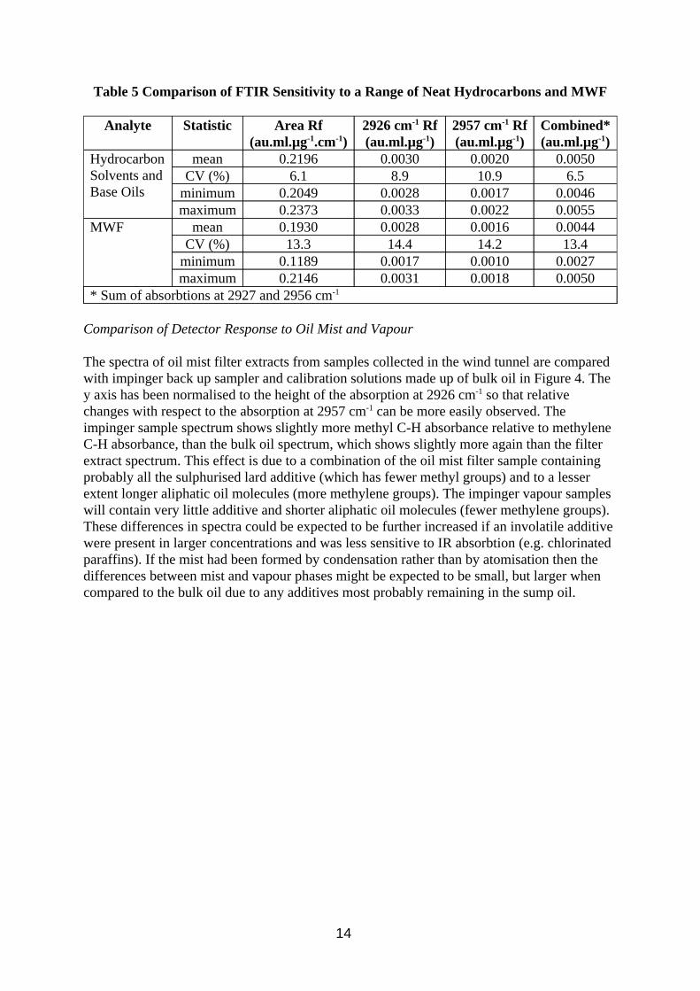
Table 5 Comparison of FTIR Sensitivity to a Range of Neat Hydrocarbons and MWF

Analyte Statistic Area Rf (au.ml.µg-1.cm-1)

2926 cm-1 Rf (au.ml.µg-1)

2957 cm-1 Rf (au.ml.µg-1)

Combined* (au.ml.µg-1)

Hydrocarbon Solvents and Base Oils

mean 0.2196 0.0030 0.0020 0.0050 CV (%) 6.1 8.9 10.9 6.5

minimum 0.2049 0.0028 0.0017 0.0046 maximum 0.2373 0.0033 0.0022 0.0055

MWF mean 0.1930 0.0028 0.0016 0.0044 CV (%) 13.3 14.4 14.2 13.4

minimum 0.1189 0.0017 0.0010 0.0027 maximum 0.2146 0.0031 0.0018 0.0050

* Sum of absorbtions at 2927 and 2956 cm-1

Comparison of Detector Response to Oil Mist and Vapour

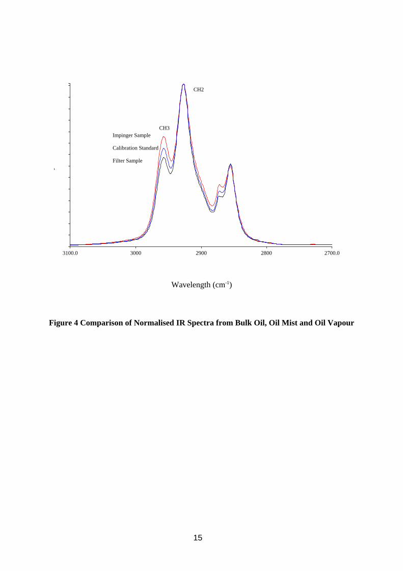
The spectra of oil mist filter extracts from samples collected in the wind tunnel are compared with impinger back up sampler and calibration solutions made up of bulk oil in Figure 4. The y axis has been normalised to the height of the absorption at 2926 cm-1 so that relative changes with respect to the absorption at 2957 cm-1 can be more easily observed. The impinger sample spectrum shows slightly more methyl C-H absorbance relative to methylene C-H absorbance, than the bulk oil spectrum, which shows slightly more again than the filter extract spectrum. This effect is due to a combination of the oil mist filter sample containing probably all the sulphurised lard additive (which has fewer methyl groups) and to a lesser extent longer aliphatic oil molecules (more methylene groups). The impinger vapour samples will contain very little additive and shorter aliphatic oil molecules (fewer methylene groups). These differences in spectra could be expected to be further increased if an involatile additive were present in larger concentrations and was less sensitive to IR absorbtion (e.g. chlorinated paraffins). If the mist had been formed by condensation rather than by atomisation then the differences between mist and vapour phases might be expected to be small, but larger when compared to the bulk oil due to any additives most probably remaining in the sump oil.

14

A

CH3

CH2

Impinger Sample

Calibration Standard

Filter Sample

3100.0 3000 2900 2800 2700.0

Wavelength (cm-1)

Figure 4 Comparison of Normalised IR Spectra from Bulk Oil, Oil Mist and Oil Vapour

15

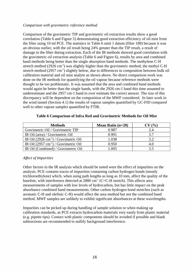
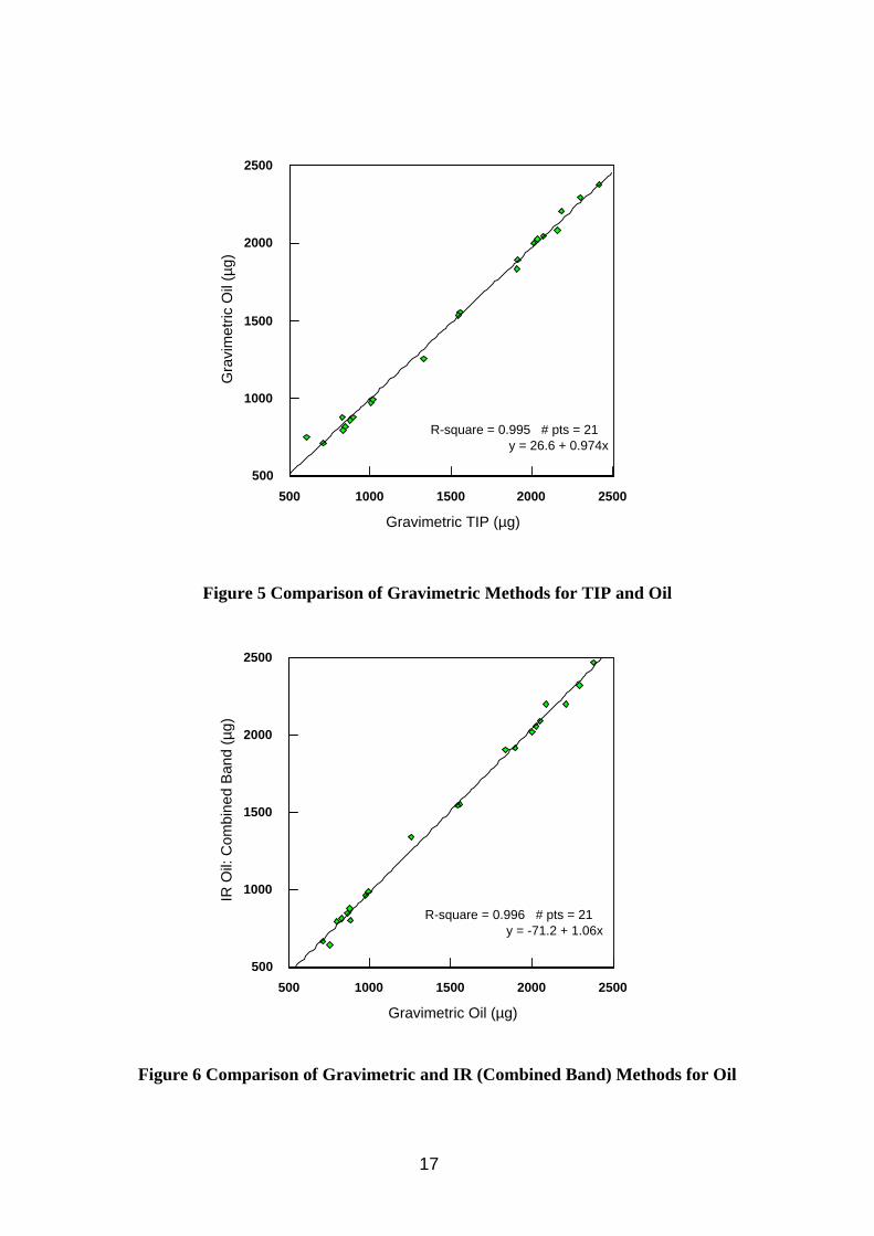
Comparison with gravimetric reference method

Comparison of the gravimetric TIP and gravimetric oil extraction results show a good correlation (Table 6 and Figure 5) demonstrating good extraction efficiency of oil mist from the filter using 10 ml PCE. The statistics in Table 6 omit 1 datum (filter 189) because it was an obvious outlier, with the oil result being 24% greater than the TIP result, a result of damage to the filter during extraction. Each of the IR methods showed good correlation with the gravimetric oil extraction analysis (Table 6 and Figure 6), results by area and combined band methods being better than the single absorption band methods. The methylene C-H stretch method (2926 cm-1) was slightly higher than the gravimetric method, the methyl C-H stretch method (2957 cm-1) slightly below, due to differences in composition between bulk oil calibration material and oil mist analyte as shown above. No direct comparison work was done on the IR methods for quantifying the oil vapour because reference methods were thought to be too problematic. It was assumed that the area and combined band methods would again be better than the single bands, with the 2926 cm-1 band this time assumed to underestimate and the 2957 cm-1 band to over estimate the correct answer. The size of this discrepancy will be dependent on the composition of the MWF considered. In later work in the wind tunnel (Section 4.1) the results of vapour samples quantified by GC-FID compared well to other vapour samples quantified by FTIR.

Table 6 Comparison of Infra Red and Gravimetric Methods for Oil Mist

Methods Mean Ratio (n=20) CV (%) Gravimetric Oil / Gravimetric TIP 0.987 2.4 IR Oil (area) / Gravimetric Oil 0.991 3.7 IR Oil (2926 cm-1) / Gravimetric Oil 1.038 3.2 IR Oil (2957 cm-1) / Gravimetric Oil 0.950 4.0 IR Oil (Combined) / Gravimetric Oil 1.005 3.5

Affect of Impurities

Other factors in the IR analysis which should be noted were the effect of impurities on the analysis. PCE contains traces of impurities containing carbon hydrogen bonds (mostly trichloroethylene) which, when using path lengths as long as 10 mm, affect the quality of the baseline, with interference detected at 2880 cm-1 (C=C-H stretch). This affects area measurements of samples with low levels of hydrocarbon, but has little impact on the peak absorbance combined band measurements. Other carbon hydrogen bond stretches (such as aromatic C-H and olefinic C-H) would affect the area method but not the combined band method. MWF samples are unlikely to exhibit significant absorbances at these wavelengths.

Impurities can be picked up during handling of sample solution or when making up calibration standards, as PCE extracts hydrocarbon materials very easily from plastic material (e.g. pipette tips). Contact with plastic components should be avoided if possible and blank subtractions are recommended to nullify background interference.

16

500

1000

1500

2000

2500

Gra

vim

etric

Oil

(µg)

R-square = 0.995 # pts = 21 y = 26.6 + 0.974x

500 1000 1500 2000 2500

Gravimetric TIP (µg)

Figure 5 Comparison of Gravimetric Methods for TIP and Oil

2500

IR O

il: C

ombi

ned

Ban

d (µ

g) 2000

1500

1000

500

R-square = 0.996 # pts = 21 y = -71.2 + 1.06x

500 1000 1500 2000 2500

Gravimetric Oil (µg)

Figure 6 Comparison of Gravimetric and IR (Combined Band) Methods for Oil

17

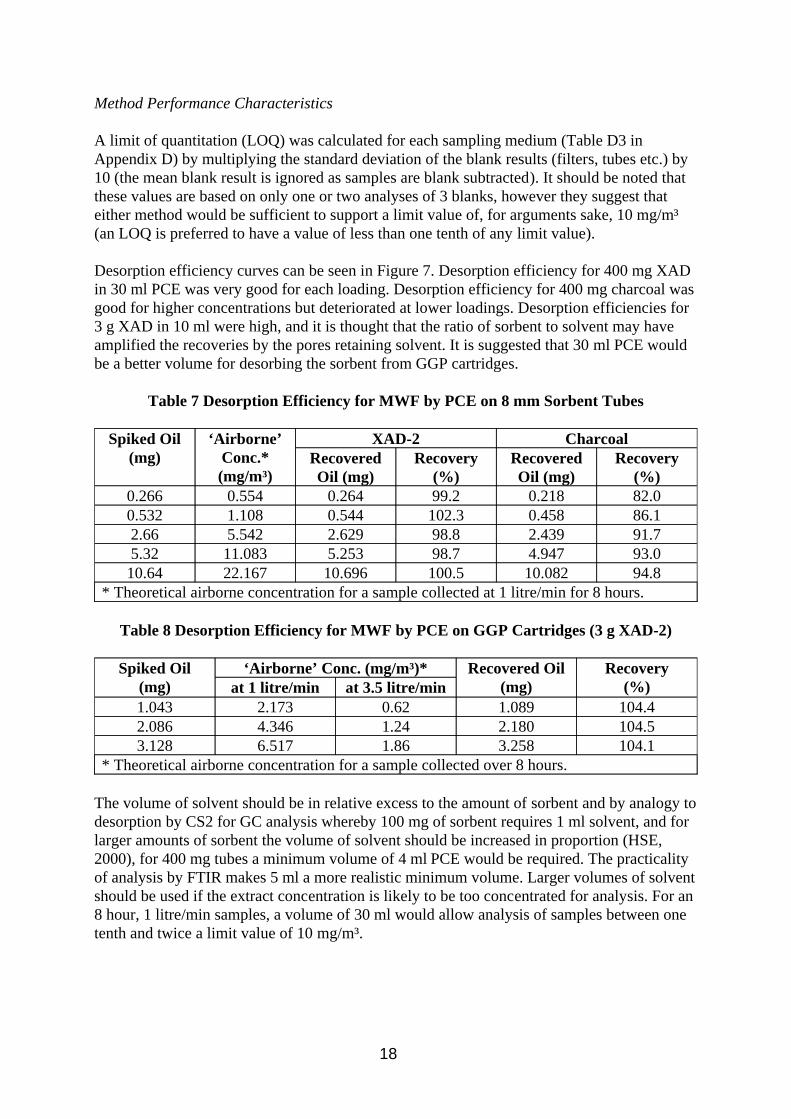
Method Performance Characteristics

A limit of quantitation (LOQ) was calculated for each sampling medium (Table D3 in Appendix D) by multiplying the standard deviation of the blank results (filters, tubes etc.) by 10 (the mean blank result is ignored as samples are blank subtracted). It should be noted that these values are based on only one or two analyses of 3 blanks, however they suggest that either method would be sufficient to support a limit value of, for arguments sake, 10 mg/m³ (an LOQ is preferred to have a value of less than one tenth of any limit value).

Desorption efficiency curves can be seen in Figure 7. Desorption efficiency for 400 mg XAD in 30 ml PCE was very good for each loading. Desorption efficiency for 400 mg charcoal was good for higher concentrations but deteriorated at lower loadings. Desorption efficiencies for 3 g XAD in 10 ml were high, and it is thought that the ratio of sorbent to solvent may have amplified the recoveries by the pores retaining solvent. It is suggested that 30 ml PCE would be a better volume for desorbing the sorbent from GGP cartridges.

Table 7 Desorption Efficiency for MWF by PCE on 8 mm Sorbent Tubes

Spiked Oil (mg)

‘Airborne’ Conc.* (mg/m³)

XAD-2 Charcoal Recovered Oil (mg)

Recovery (%)

Recovered Oil (mg)

Recovery (%)

0.266 0.554 0.264 99.2 0.218 82.0 0.532 1.108 0.544 102.3 0.458 86.1 2.66 5.542 2.629 98.8 2.439 91.7 5.32 11.083 5.253 98.7 4.947 93.0 10.64 22.167 10.696 100.5 10.082 94.8

* Theoretical airborne concentration for a sample collected at 1 litre/min for 8 hours.

Table 8 Desorption Efficiency for MWF by PCE on GGP Cartridges (3 g XAD-2)

Spiked Oil (mg)

‘Airborne’ Conc. (mg/m³)* Recovered Oil (mg)

Recovery (%)at 1 litre/min at 3.5 litre/min

1.043 2.173 0.62 1.089 104.4 2.086 4.346 1.24 2.180 104.5 3.128 6.517 1.86 3.258 104.1

* Theoretical airborne concentration for a sample collected over 8 hours.

The volume of solvent should be in relative excess to the amount of sorbent and by analogy to desorption by CS2 for GC analysis whereby 100 mg of sorbent requires 1 ml solvent, and for larger amounts of sorbent the volume of solvent should be increased in proportion (HSE, 2000), for 400 mg tubes a minimum volume of 4 ml PCE would be required. The practicality of analysis by FTIR makes 5 ml a more realistic minimum volume. Larger volumes of solvent should be used if the extract concentration is likely to be too concentrated for analysis. For an 8 hour, 1 litre/min samples, a volume of 30 ml would allow analysis of samples between one tenth and twice a limit value of 10 mg/m³.

18

110

100

105 R

ecov

ery

(%)

95

90

85

80

400 mg charcoal / 30 ml 400 mg XAD / 30 ml 3 g XAD / 10 ml

0 2 4 6 8 10 12

Oil Recovered (mg)

Figure 7 PCE Desorption Efficiency Curve

3.2.4. Conclusion

w FTIR can be used to quantify both mist and vapour phases of the airborne oil.

w FTIR was more sensitive to the base oils and other hydrocarbon solvents tested than to those MWF tested, due to the presence of the additives in the MWF.

w The range of detector response is wider for MWF than for the base oils due to the different types and amounts of additives present.

w The IR spectra of mist and vapour samples may vary from that of the bulk material due to the unequal distribution of material between the two phases, with additives and larger hydrocarbons being mostly in the mist phase, and the lighter hydrocarbons being in the vapour phase.

w It is recommended that calibration should ideally be against MWF from the sump of the machine in question.

w FTIR cannot distinguish between oil vapour and any other unrelated hydrocarbon material sampled (e.g. white spirit type solvents, ethyl acetate etc.).

w Measurement of oil mist from the total area of the C-H bond stretches or by combination of peak absorbances of the larger bands at ~2957 and 2926 cm-1

(methyl and methylene C-H stretches) was found to be more accurate than

19

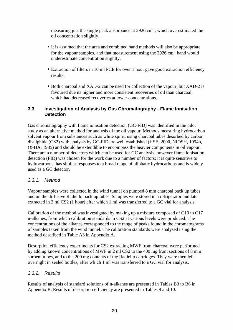
measuring just the single peak absorbance at 2926 cm-1, which overestimated the oil concentration slightly.

w It is assumed that the area and combined band methods will also be appropriate for the vapour samples, and that measurement using the 2926 cm-1 band would underestimate concentration slightly.

w Extraction of filters in 10 ml PCE for over 1 hour gave good extraction efficiency results.

w Both charcoal and XAD-2 can be used for collection of the vapour, but XAD-2 is favoured due its higher and more consistent recoveries of oil than charcoal, which had decreased recoveries at lower concentrations.

3.3. Investigation of Analysis by Gas Chromatography - Flame Ionisation Detection

Gas chromatography with flame ionisation detection (GC-FID) was identified in the pilot study as an alternative method for analysis of the oil vapour. Methods measuring hydrocarbon solvent vapour from substances such as white spirit, using charcoal tubes desorbed by carbon disulphide (CS2) with analysis by GC-FID are well established (HSE, 2000, NIOSH, 1994b, OSHA, 1985) and should be extendible to encompass the heavier components in oil vapour. There are a number of detectors which can be used for GC analysis, however flame ionisation detection (FID) was chosen for the work due to a number of factors; it is quite sensitive to hydrocarbons, has similar responses to a broad range of aliphatic hydrocarbons and is widely used as a GC detector.

3.3.1. Method

Vapour samples were collected in the wind tunnel on pumped 8 mm charcoal back up tubes and on the diffusive Radiello back up tubes. Samples were stored in a refrigerator and later extracted in 2 ml CS2 (1 hour) after which 1 ml was transferred to a GC vial for analysis.

Calibration of the method was investigated by making up a mixture composed of C10 to C17 n-alkanes, from which calibration standards in CS2 at various levels were produced. The concentrations of the alkanes corresponded to the range of peaks found in the chromatograms of samples taken from the wind tunnel. The calibration standards were analysed using the method described in Table A3 in Appendix A.

Desorption efficiency experiments for CS2 extracting MWF from charcoal were performed by adding known concentrations of MWF in 2 ml CS2 to the 400 mg front sections of 8 mm sorbent tubes, and to the 200 mg contents of the Radiello cartridges. They were then left overnight in sealed bottles, after which 1 ml was transferred to a GC vial for analysis.

3.3.2. Results

Results of analysis of standard solutions of n-alkanes are presented in Tables B3 to B6 in Appendix B. Results of desorption efficiency are presented in Tables 9 and 10.

20

3.3.3. Discussion

Method Calibration

Samples collected on back up tubes behind filters will comprise of material that easily vaporises, and so will present no problem for analysis by GC, however filter samples or samples collected on pumped sorbent tubes with no preceding filter may not be suitable for GC analysis. Such samples may contain involatile material such as high molecular weight oil components and MWF additives which will not be vaporised easily and so will not be detected by GC analysis. Enquiries to 3 MWF manufacturers revealed that, estimating from the flash points of the neat materials, additives are most likely to be in the particulate phase (Table C4, Appendix C). The common alkanes found in the oil vapour (C13 to C16) have flash points between 79 and 135°C, whereas the additives’ flash points are generally somewhat higher.

Oil vapour samples are expected to comprise mostly of aliphatic material between C12 and C17, however if hydrocarbon solvents are present, originating from either separate materials or from within the MWF, then the range may start at C8 or lower.

In other methods for hydrocarbon solvents, calibration has used the analyte sampled as calibration material, and the calibration has been on the summed areas of the peaks (NIOSH 1994b, OSHA, 1985). The OSHA method adds that if the material is coloured or is denser than 0.79 g/ml then it needs to be distilled to separate the solvent from pigments or heavier oil, but does not specify a boiling point cut off point. It suggests that as similar response to different hydrocarbons are observed for FIDs, a substitute solvent of the same type could be used for calibration. In MDHS 66, an analogous HSE method (HSE, 1994) for mixed hydrocarbons (C5 to C10) using thermal desorption, n-heptane (C7) is used for all aliphatic hydrocarbons and toluene for all aromatic hydrocarbons provided that relative response factors are within 15%.

For oil vapour samples, the vapour will represent only a fraction of the bulk material. The bulk material contains some components found only in the mist phase and other more volatile components found in both phases. Distillation would be an impracticable and lengthy (also costly) additional step in the analysis, especially if an acceptable alternative method was available. To simplify calibration, all peaks in the chromatogram were assumed to be aliphatic hydrocarbons and calibration was made on the sum of the peaks. Additives (e.g. fatty acid methyl esters) and aromatic compounds can be present in the vapour phase and will have differing detector responses, however these are likely to represent a very small proportion of vapour samples. Confirmation of the identity of peaks could be made by subsequent analysis by mass spectrometry if available. Components in the sample are likely to cover a wide range of boiling points and so internal standards were not used. Modern auto-injectors for gas chromatographs provide a high level of repeatability, and if care is taken to minimise the evaporation of CS2, then there should be only small errors in the analysis. The detector was found to be linear over a very wide range of concentrations for each analyte, as can be seen from the examples of calibration curves for tetradecane (nC14) in Figure 8 and 9. Response factors varied little between the alkanes tested, nC10 being slightly less than later eluting compounds due to small losses in the injection system. Response factors were also consistent

21

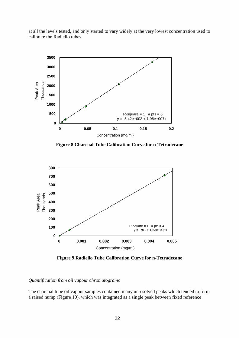
at all the levels tested, and only started to vary widely at the very lowest concentration used to calibrate the Radiello tubes.

0

500

1000

1500

2000

2500

3000

3500

Thou

sand

sP

eak

Are

a

R-square = 1 # pts = 6 y = -5.42e+003 + 1.98e+007x

0 0.05 0.1 0.15 0.2

Concentration (mg/ml)

Figure 8 Charcoal Tube Calibration Curve for n-Tetradecane

800

0 0.001 0.002 0.003 0.004 0.005

Concentration (mg/ml)

Figure 9 Radiello Tube Calibration Curve for n-Tetradecane

0

100

200

300

400

500

600

700

Thou

sand

sPe

ak A

rea

R-square = 1 # pts = 4 y = -701 + 1.53e+008x

Quantification from oil vapour chromatograms

The charcoal tube oil vapour samples contained many unresolved peaks which tended to form a raised hump (Figure 10), which was integrated as a single peak between fixed reference

22

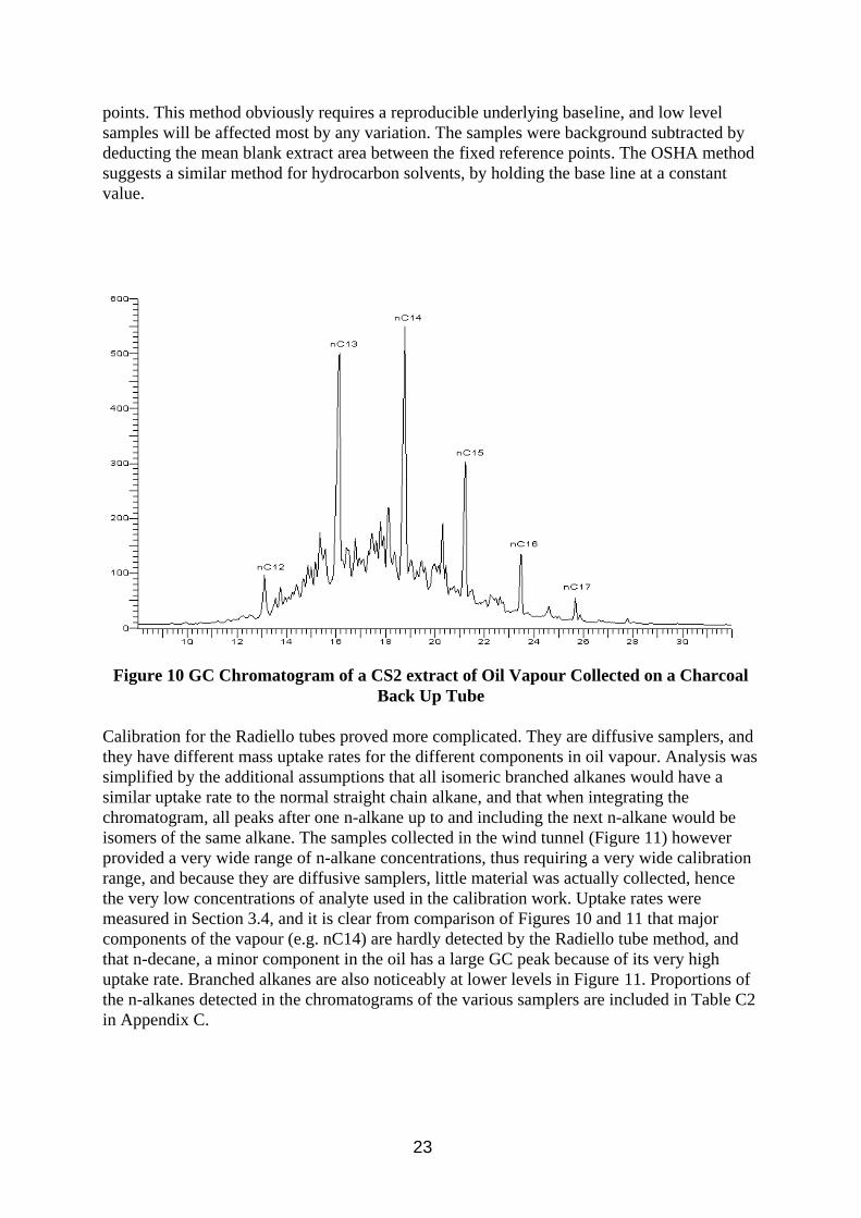
points. This method obviously requires a reproducible underlying baseline, and low level samples will be affected most by any variation. The samples were background subtracted by deducting the mean blank extract area between the fixed reference points. The OSHA method suggests a similar method for hydrocarbon solvents, by holding the base line at a constant value.

Figure 10 GC Chromatogram of a CS2 extract of Oil Vapour Collected on a Charcoal Back Up Tube

Calibration for the Radiello tubes proved more complicated. They are diffusive samplers, and they have different mass uptake rates for the different components in oil vapour. Analysis was simplified by the additional assumptions that all isomeric branched alkanes would have a similar uptake rate to the normal straight chain alkane, and that when integrating the chromatogram, all peaks after one n-alkane up to and including the next n-alkane would be isomers of the same alkane. The samples collected in the wind tunnel (Figure 11) however provided a very wide range of n-alkane concentrations, thus requiring a very wide calibration range, and because they are diffusive samplers, little material was actually collected, hence the very low concentrations of analyte used in the calibration work. Uptake rates were measured in Section 3.4, and it is clear from comparison of Figures 10 and 11 that major components of the vapour (e.g. nC14) are hardly detected by the Radiello tube method, and that n-decane, a minor component in the oil has a large GC peak because of its very high uptake rate. Branched alkanes are also noticeably at lower levels in Figure 11. Proportions of the n-alkanes detected in the chromatograms of the various samplers are included in Table C2 in Appendix C.

23

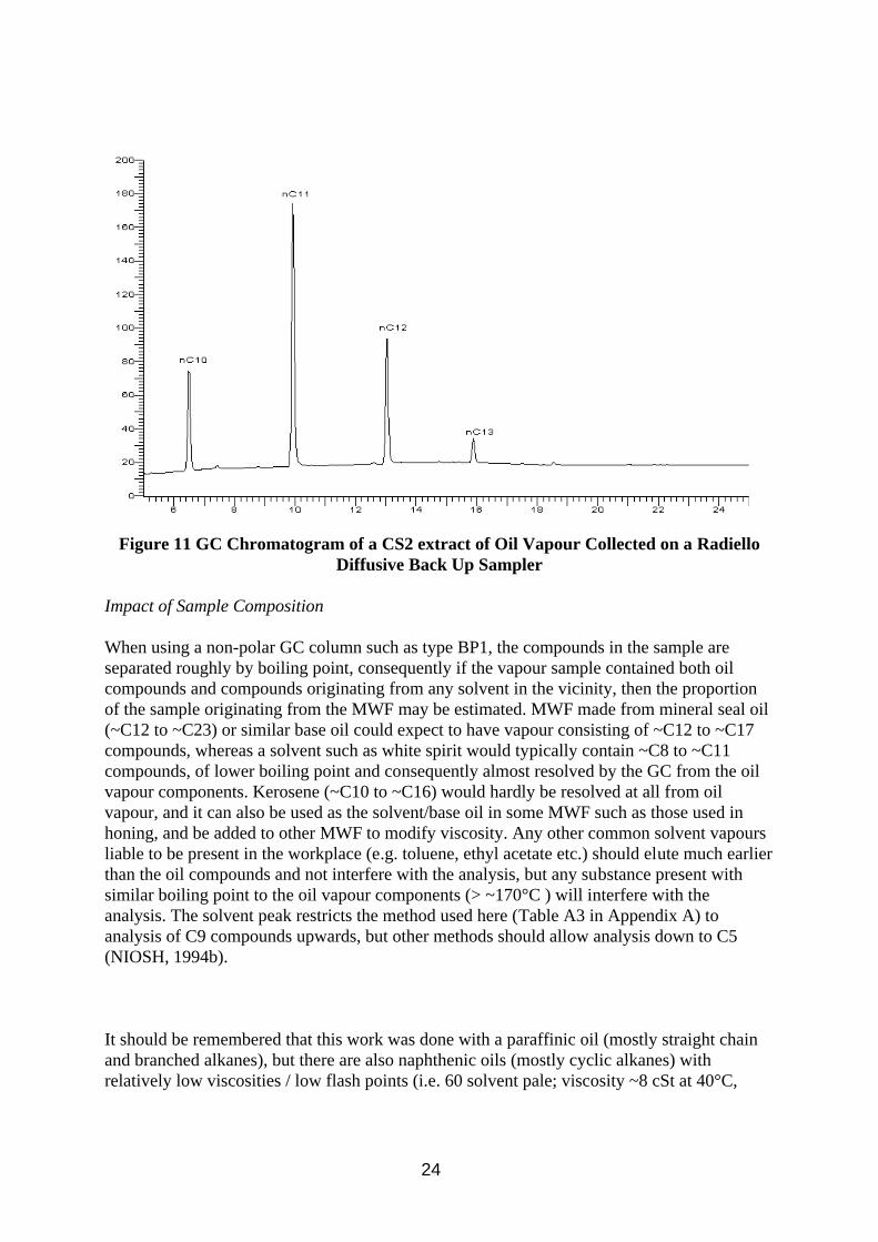
Figure 11 GC Chromatogram of a CS2 extract of Oil Vapour Collected on a Radiello Diffusive Back Up Sampler

Impact of Sample Composition

When using a non-polar GC column such as type BP1, the compounds in the sample are separated roughly by boiling point, consequently if the vapour sample contained both oil compounds and compounds originating from any solvent in the vicinity, then the proportion of the sample originating from the MWF may be estimated. MWF made from mineral seal oil (~C12 to ~C23) or similar base oil could expect to have vapour consisting of ~C12 to ~C17 compounds, whereas a solvent such as white spirit would typically contain ~C8 to ~C11 compounds, of lower boiling point and consequently almost resolved by the GC from the oil vapour components. Kerosene (~C10 to ~C16) would hardly be resolved at all from oil vapour, and it can also be used as the solvent/base oil in some MWF such as those used in honing, and be added to other MWF to modify viscosity. Any other common solvent vapours liable to be present in the workplace (e.g. toluene, ethyl acetate etc.) should elute much earlier than the oil compounds and not interfere with the analysis, but any substance present with similar boiling point to the oil vapour components (> ~170°C ) will interfere with the analysis. The solvent peak restricts the method used here (Table A3 in Appendix A) to analysis of C9 compounds upwards, but other methods should allow analysis down to C5 (NIOSH, 1994b).

It should be remembered that this work was done with a paraffinic oil (mostly straight chain and branched alkanes), but there are also naphthenic oils (mostly cyclic alkanes) with relatively low viscosities / low flash points (i.e. 60 solvent pale; viscosity ~8 cSt at 40°C,

24

flash point 145°C), which should have accompanying vapour when misting. Such oils have no resolved peaks such as in Figure 10, but a relatively featureless hydrocarbon envelope due to the number and relative quantities of the component compounds. They can be analysed by GC but the chromatograms will not be as easy to interpret as for paraffinic oils or to integrate. It is easier to integrate chromatograms with distinct peaks, and the n-alkane peaks in paraffinic oils help characterise the distribution of components in the sample by boiling point range.

Method Performance Characteristics

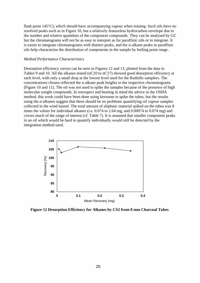
Desorption efficiency curves can be seen in Figures 12 and 13, plotted from the data in Tables 9 and 10. All the alkanes tested (nC10 to nC17) showed good desorption efficiency at each level, with only a small drop at the lowest level used for the Radiello samplers. The concentrations chosen reflected the n-alkane peak heights in the respective chromatograms (Figure 10 and 11). The oil was not used to spike the samples because of the presence of high molecular weight compounds. In retrospect and bearing in mind the advice in the OSHA method, this work could have been done using kerosene to spike the tubes, but the results using the n-alkanes suggest that there should be no problems quantifying oil vapour samples collected in the wind tunnel. The total amount of aliphatic material spiked on the tubes was 8 times the values for individual alkanes (i.e. 0.074 to 2.64 mg, and 0.00074 to 0.074 mg) and covers much of the range of interest (cf. Table 7). It is assumed that smaller component peaks in an oil which would be hard to quantify individually would still be detected by the integration method used.

Rec

over

y (%

)

110

105

100

95

90

85

80 0 0.1 0.2 0.3 0.4

Mean Recovery (mg)

Figure 12 Desorption Efficiency for Alkanes by CS2 from 8 mm Charcoal Tubes

25

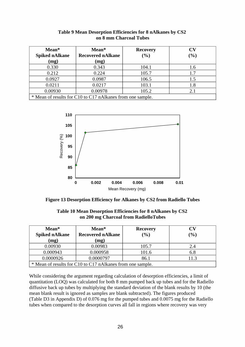
Table 9 Mean Desorption Efficiencies for 8 nAlkanes by CS2 on 8 mm Charcoal Tubes

Mean* Spiked nAlkane

(mg)

Mean* Recovered nAlkane

(mg)

Recovery (%)

CV (%)

0.330 0.343 104.1 1.6 0.212 0.224 105.7 1.7 0.0927 0.0987 106.5 1.5 0.0211 0.0217 103.1 1.8 0.00930 0.00978 105.2 2.1

* Mean of results for C10 to C17 nAlkanes from one sample.

0 0.002 0.004 0.006 0.008 0.01 Mean Recovery (mg)

Figure 13 Desorption Efficiency for Alkanes by CS2 from Radiello Tubes

Table 10 Mean Desorption Efficiencies for 8 nAlkanes by CS2 on 200 mg Charcoal from RadielloTubes

80

85

90

95

100

105

110

Rec

over

y (%

)

Mean* Spiked nAlkane

(mg)

Mean* Recovered nAlkane

(mg)

Recovery (%)

CV (%)

0.00930 0.00983 105.7 2.4 0.000943 0.000958 101.6 6.8 0.0000926 0.0000797 86.1 11.3

* Mean of results for C10 to C17 nAlkanes from one sample.

While considering the argument regarding calculation of desorption efficiencies, a limit of quantitation (LOQ) was calculated for both 8 mm pumped back up tubes and for the Radiello diffusive back up tubes by multiplying the standard deviation of the blank results by 10 (the mean blank result is ignored as samples are blank subtracted). The figures produced (Table D3 in Appendix D) of 0.076 mg for the pumped tubes and 0.0075 mg for the Radiello tubes when compared to the desorption curves all fall in regions where recovery was very

26

high. The pumped tube LOQ corresponds to an airborne figure of 0.158 mg/m³ for an 8 hour sample collected at 1 litre/min. It should be noted that this value is based on only one analysis of 3 blanks, however they suggest that the method would be sufficient to support a limit value such as 10 mg/m³. Converting the Radiello tube LOQ to an equivalent airborne concentration requires an uptake value for each compound. Assuming that all isomers of an alkane have similar uptake rates, then using the values calculated in Section 3.4 for C10 to C14 the airborne equivalent for an 8 hour exposure would be 9.01 mg/m³. This exceptionally high figure is mostly due to the low uptake rates at higher molecular weight; C13 and C14 make up 98% of the total. If C15 to C18 were included then the total would be even higher.

3.3.4. Conclusion

w GC-FID can be used to quantify oil vapour but not oil mist or total oil. MWF oil mist is likely to contain heavy oil components and additives which will not be sufficiently volatile to be vaporised and / or chromatographed effectively. Oils which do not contain such components may be able to be analysed by GC-FID.

w Calibration with the oil in question is unworkable unless a fraction roughly equivalent to the vapour is distilled off. Substitution with kerosene may prove to be possible.

w Paraffinic alkanes between C10 and C17 have similar response factors when analysed by FID. Aromatics and oil additives will have varying response factors, but they are likely to represent only a very small proportion of the vapour sample. Therefore calibration on the sum of the peak integrations is possible.

w Analysis could be calibrated by a single n-alkane (e.g. n-tetradecane), however it would be good practise to include other alkanes to ensure effective chromatography over a wide boiling point range.

w Desorption efficiency of alkanes between C10 and C17 from charcoal was effective with CS2.

w Most solvents captured during sampling should not interfere with the analysis, but any substance present with similar boiling point to the oil vapour components (> ~170°C) is likely to interfere interfere with the analysis (e.g. white spirit).

3.4. Investigation of Diffusive Sampling

Diffusive sampling was included in this work as it was seen as a potential method which could differentiate between mist and vapour. If a diffusive sampler method could measure vapour accurately and pumped samplers could measure total oil accurately then the difference would be due to the mist. Potential problems envisaged are low levels of sample collected due to the relatively low vapour concentrations present (when compared to solvent analysis), splashing from the oil during use, and possible diffusion of small particles into the sampler. Open face badge type diffusive samplers would be vulnerable to splashing, as would cylindrical Radiello samplers. Thus all work on separate diffusuve samplers was done on tube type samplers. Thermal desorption analysis was chosen over solvent desorption to increase

27

method sensitivity and Tenax was chosen as sorbent as it can withstand temperatures up to 300°C during desorption, thought desirable for good desorption efficiency of higher molecular weight components.

Diffusive samplers were also considered as back up samplers to filter sampling. There are concerns that commercially available sorbent tubes would be incompatible with the flow rates used for filter sampling due to potential problems with overloading or channelling in the sorbent, breakthrough of the analyte or high pump back pressure, and diffusive sampling was seen as a potential solution. There are no commercially available equipment for achieving this arrangement, but a design has been developed at HSE utilising a Radiello tube inside a metal canister (Section 2.2.4), and a similar arrangement with a Perkin Elmer ATD tube has been developed by other researchers (Lichtenstein et al, 1997). The Radiello tube arrangement was chosen for testing because it has a higher sampling rate (the quoted uptake rate for n-decane is 100 times higher than for the ATD tube). The sorbent chosen was charcoal, solvent desorbed by CS2 as per the manufacturer’s instructions. XAD-2 extracts contained impurities which obscured analyte peaks, and Tenax is said to be incompatible with CS2., although other solvents may have been suitable.

The diffusive uptake rate of a compound is required if its airborne concentration is to be calculated from the amount sampled. Although theoretical uptake rates can be calculated, ideally analyte concentrations should be determined using measured uptake rates. Published diffusive uptake rates for Tenax ATD tubes exist in the literature (HSE, 1994) for C7 to C10 n-alkanes but not for heavier compounds. Similarly Radiello tube uptake rates only exist for C6 to C8 and C10 n-alkanes. Oil vapour composition is likley to extend to at least C17 alkanes, and this work intends to investigate these heacier compounds.

A second aim for this work is to investigate the extent that the oil mist particles may interfere with the vapour analysis. Any mist sampled would contribute to and bias the vapour concentration calculated.

3.4.1. Method

Method calibration

The analysis of oil vapour samples by ATD-GC-FID was investigated by analysing spiked Tenax tubes. The tubes were spiked by injecting a solution composing equal parts of n-alkanes between C10 and C17 in methanol onto the tube and then evaporating the methanol by blowing nitrogen through the tube. The spiked tubes were used to develop a method and then investigate calibration and desorption efficiency.

Uptake Rates

The n-alkane mixture was used to create a standard atmosphere described in Section 2.2.2. Inside the atmosphere were placed 6 diffusive Tenax ATD tubes, 6 Radiello tubes (positioned behind multi-orifice samplers with GF/A filters pumped at 2 litres/min), and 6 pumped Tenax ATD tubes (10 ml/min) as a reference method. The test was run for 4 hours and 8 hours under the conditions described in Tabe A4 in Appendix A, after which the samples were stored in a refrigerator. The diffusive and pumped Tenax tubes were analysed by ATD-GC-FID using the

28

instrumental conditions in Table A5 in Appendix A. The diffusive tubes were analysed using a split of ~12% to get maximum sensitivity, the pumped tubes were analysed at a split of ~1%. The Radiello tubes were extracted in 2 ml CS2 and analysed by GC-FID using the instrumental conditions in Table A3 in Appendix A.

Effect of oil mist particles on vapour measurements

To investigate the effect of oil mist particles on the diffusive sampling of oil vapour, the tenax tubes were exposed in the wind tunnel using the conditions in Table A1, Appendix A. Six samplers were exposed with the sampling caps pointing upwards, and six more with the caps pointing downwards. An additional six empty tubes (apart from retaining metal gauze) were exposed facing upwards and six more facing downwards. Three filter samplers with back up impingers (described in Section 2.1.1) were present as reference method. Samples collected were stored in a refrigerator. The diffusive tubes plus 3 blank tubes were analysed by ATD-GC-FID as above, and the filters and impingers by FTIR (using conditions described in Table A2, Appendix A). The filters were extracted in 10 ml PCE over night alongside 3 blank filters. The blank filter extracts were used to background subtract the sample filters, and solvent blanks were used to background subtract the impinger samples.

3.4.2. Results

The results of work looking at analysis of oil vapour by ATD-GC-FID are presented in Tables B7 and B8 in Appendix B.

The results of the experiments to measure the uptake rates are presented in Table B9 in Appendix B and the calculated uptake rates summarised in Table 11.

The results of the wind tunnel work investigating particle effects are summarised in Table 12. The particle size characterisation results are included in Table D1, Appendix D.

3.4.3. Discussion

Method Calibration

Many of the considerations for analysis by GC-FID from Section 3.3 also apply to analysis by ATD-GC-FID. Samples should comprise of material that easily vaporises and thus present no problem to analysis by GC. However if mist has entered the ATD tube then involatile material such as high molecular weight oil components and MWF additives may be present. Some of this material will not be detected, but some will be detected (perhaps poorly) and be indistinguishable from the vapour components. The big difference for analysis by ATD-GC-FID is that the sample undergoes a two stage thermal desorption during which sample maybe lost. Calibration of the FID has exactly the same considerations as Section 3.3, and the intention was to calibrate on a single n-alkane as per MDHS 66, (HSE method for mixed hydrocarbons (C5 to C10) using thermal desorption (HSE, 1994)), assuming the bulk of the sample to be aliphatic hydrocarbons, and that isomers of the n-alkanes would have similar uptake rates.

29

Response factors were consistent over a wide range of concentrations for each alkane tested, indicating good recovery from the ATD tubes and chromatography on the GC. The GC peak shape started to deteriorate at nC17 and was hard to integrate accurately at the lower concentration level, and hence its higher and more varied mean response factor. Components heavier than nC17 are likely to be more greatly affected, but are likely to constitute a very small proportion of the sample. Analysis with a shorter GC column or one capable of higher GC oven temperatures may improve chromatography. Response factors did vary more at the lower calibration level due to the small size of the peaks, however little can be done to increase peak size as the instrument was already set for maximum sensitivity. Consequently a mean response factor used was calculated from the upper two concentration levels.

Uptake Rates

The experiments to measure sampler uptake rates experienced some problems. The standard atmospheres of the n-alkanes were created using a mixture of n-alkanes in equal proportion but because of the decreasing volatility of the compounds with molecular weight, the resulting atmosphere created showed a decline in concentration as the alkanes became less volatile (Table B9). The decreasing analyte concentration is accompanied by increasing variation of the means of the results, and when the calculated uptake values are plotted graphically (Figures 12 and 13), it is apparent that due to this drop in accuracy the trend which can be seen for lighter alkanes dissipates at higher molecular weight. Some values are quite clearly unsound, being anomalous with the earlier trend, higher than lighter compounds or even negative (due to blank subtraction) and it is clear that they are not sufficiently accurate and so appear in Table 11 only for the sake of completeness and have been crossed out. These compounds were present at low concentrations and were hard to measure with the same level of accuracy as other more concentrated alkanes. Decane (C10) is the only compound with published uptake values for comparison. The ATD tube experimental values are at 80 and 85 %, and the Radiello tube at 70 and 78 % of the respective published values. One possible reason for the decreased uptake rate could be the presence of the other alkanes in the sampled atmosphere. Both the 4 hour and 8 hour values are relatively consistent with each other and fit a trend with C11 to C13 alkanes (Figures 14 and 15).

30

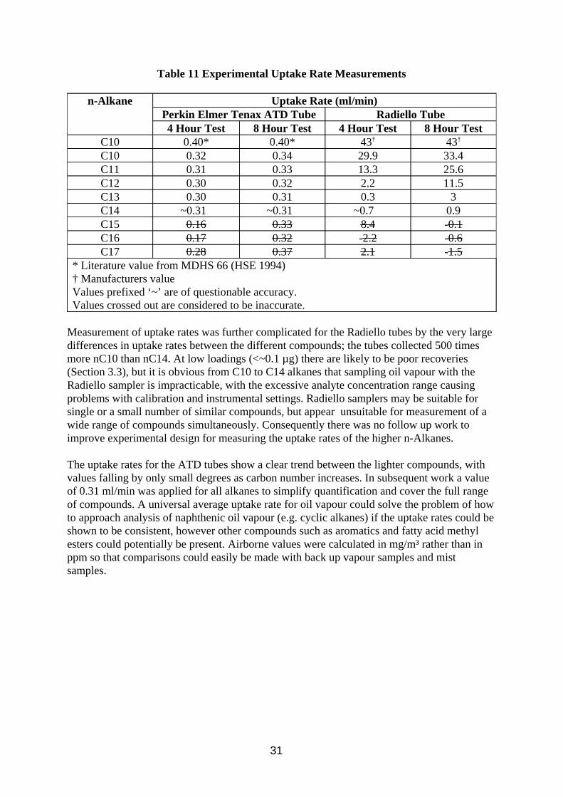
Table 11 Experimental Uptake Rate Measurements

n-Alkane Uptake Rate (ml/min) Perkin Elmer Tenax ATD Tube Radiello Tube 4 Hour Test 8 Hour Test 4 Hour Test 8 Hour Test

C10 0.40* 0.40* 43† 43†

C10 0.32 0.34 29.9 33.4 C11 0.31 0.33 13.3 25.6 C12 0.30 0.32 2.2 11.5 C13 0.30 0.31 0.3 3 C14 ~0.31 ~0.31 ~0.7 0.9 C15 0.16 0.33 8.4 -0.1 C16 0.17 0.32 -2.2 -0.6 C17 0.28 0.37 2.1 -1.5

* Literature value from MDHS 66 (HSE 1994) † Manufacturers value Values prefixed ‘~’ are of questionable accuracy. Values crossed out are considered to be inaccurate.

Measurement of uptake rates was further complicated for the Radiello tubes by the very large differences in uptake rates between the different compounds; the tubes collected 500 times more nC10 than nC14. At low loadings (<~0.1 µg) there are likely to be poor recoveries (Section 3.3), but it is obvious from C10 to C14 alkanes that sampling oil vapour with the Radiello sampler is impracticable, with the excessive analyte concentration range causing problems with calibration and instrumental settings. Radiello samplers may be suitable for single or a small number of similar compounds, but appear unsuitable for measurement of a wide range of compounds simultaneously. Consequently there was no follow up work to improve experimental design for measuring the uptake rates of the higher n-Alkanes.

The uptake rates for the ATD tubes show a clear trend between the lighter compounds, with values falling by only small degrees as carbon number increases. In subsequent work a value of 0.31 ml/min was applied for all alkanes to simplify quantification and cover the full range of compounds. A universal average uptake rate for oil vapour could solve the problem of how to approach analysis of naphthenic oil vapour (e.g. cyclic alkanes) if the uptake rates could be shown to be consistent, however other compounds such as aromatics and fatty acid methyl esters could potentially be present. Airborne values were calculated in mg/m³ rather than in ppm so that comparisons could easily be made with back up vapour samples and mist samples.

31

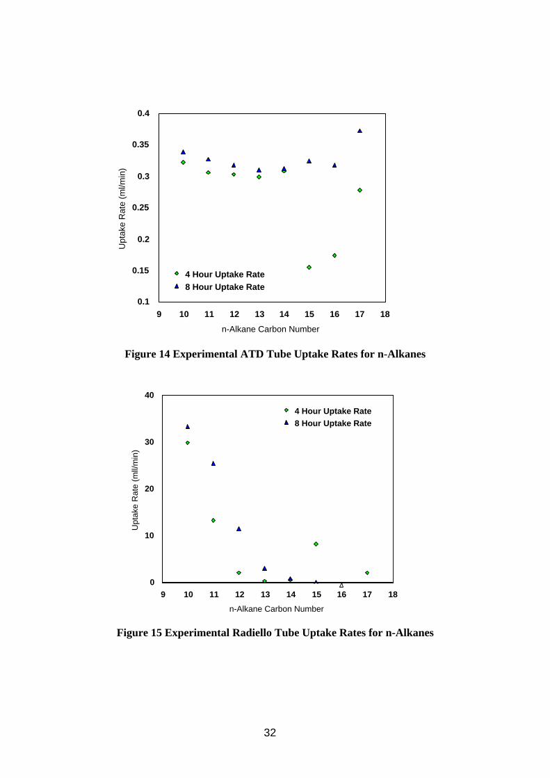
0.4

0.35

0.1 9 10 11 12 13 14 15 16 17 18

n-Alkane Carbon Number

0.15

0.2

0.25

0.3

Upt

ake

Rat

e (m

l/min

)

4 Hour Uptake Rate 8 Hour Uptake Rate

Figure 14 Experimental ATD Tube Uptake Rates for n-Alkanes

40

Upt

ake

Rat

e (m

ll/m

in)

30

20

10

0

4 Hour Uptake Rate 8 Hour Uptake Rate

9 10 11 12 13 14 15 16 17 18

n-Alkane Carbon Number

Figure 15 Experimental Radiello Tube Uptake Rates for n-Alkanes

32

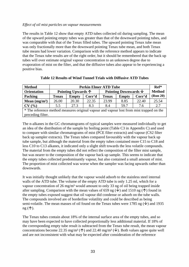
Effect of oil mist particles on vapour measurements

The results in Table 12 show that empty ATD tubes collected oil during sampling. The mean of the upward pointing empty tubes was greater than that of the downward pointing tubes, and was comparable with that of the Tenax filled tubes. The upward pointing Tenax tube mean was only fractionally more than the downward pointing Tenax tube mean, and both Tenax tube means had lower variation. Comparison with the reference method appears to indicate that the Tenax tube results are of the right order, but it should be remembered that the back up tubes will over estimate original vapour concentration to an unknown degree due to evaporation of mist on the filter, and that the diffusive tubes also appear to be experiencing a positive bias.

Table 12 Results of Wind Tunnel Trials with Diffusive ATD Tubes

Method Perkin Elmer ATD Tube Ref* Method (Run 20)

Orientation Pointing Upwards Ç Pointing Downwards È Packing Tenax Empty Corr’d Tenax Empty Corr’d Mean (mg/m³) 26.00 20.30 22.35 23.99 8.85 22.40 25.54 CV (%) 5.5 27.3 8.3 8.4 59.7 7.6 2.7 * The reference method measures original vapour and vapour lost from mist trapped on the preceding filter.

The n-alkanes in the GC chromatograms of typical samples were measured individually to get an idea of the distribution of the sample by boiling point (Table C3 in Appendix C) and used to compare with similar chromatograms of mist (PCE filter extracts) and vapour (CS2 filter back up sampler extracts). The Tenax tubes compared favourably with the vapour back up tube sample, but although the material from the empty tubes contained more C15 to C18 and less C10 to C13 alkanes, it indicated only a slight shift towards the less volatile compounds. The material from the empty tubes did not reflect the composition of the filter mist sample, but was nearer to the composition of the vapour back up sample. This seems to indicate that the empty tubes collected predominantly vapour, but also contained a small amount of mist. The proportion of mist collected was worse when the sampler was facing upwards rather than downwards.

It was initially thought unlikely that the vapour would adsorb to the stainless steel internal walls of the ATD tube. The volume of the empty ATD tube is only 1.25 ml, which for a vapour concentration of 26 mg/m³ would amount to only 33 ng of oil being trapped inside after sampling. Comparison with the mean values of 659 ng (È) and 1510 ng (Ç) found in the empty tubes exposed suggest that oil vapour did condense or adsorb on the tube walls. The compounds involved are of borderline volatility and could be described as being semi-volatile. The mean masses of oil found on the Tenax tubes were 1785 ng (È) and 1935 ng (Ç).

The Tenax tubes contain about 18% of the internal surface area of the empty tubes, and so may have been expected to have collected proportionally less additional material. If 18% of the corresponding empty tube result is subtracted from the Tenax tube result, the mean vapour concentrations become 22.35 mg/m³ (Ç) and 22.40 mg/m³ (È). Both values agree quite well and are not inconsistent with what may be expected after consideration of the reference

33

method result (the true vapour concentration is expected to be slightly less than the reference method result due to the presence of additional oil vapour originating from the mist trapped on the preceding filter).

An instrumental LOQ was calculated based on the analysis of 3 blank tenax tubes and was found to be 59 ng (corresponding to 0.39 mg/m³ over an 8 hour exposure period), suggesting that diffusive ATD tubes may have adequate sensitivity for oil vapour despite their relativley low uptake rates. This contains no contribution from analysis of empty tubes (which were themselves highly variable), if background subtraction for oil collection on internal walls was to be used.

Using diffusive sampling to differentiate oil mist / vapour mixtures looks like it could be possible but would complicate the analysis somewhat by requiring several checks. Like filter samples they would be vulnerable to splashing from the machining operation, and it would be hoped that any splashed tubes would be easy to identify. Ideally a redesigned empty tube would need to be worn next to the Tenax tube to account for additional oil collected on internal walls. After two levels of background subtraction, the accuracy of the resulting mist concentration maybe too adversely affected. More work is required on uptake rates (mixtures of compounds and naphthenic compounds) and condensation of oil vapour on internal walls before the potential for diffusive sampling can be determined. Diffusive sampling may provide a way of quantifying white spirit vapour present with the oil vapour by offering the chance to analyse the full range of compounds likely to be present (analysis of samples in PCE would be unable to quantify C8 to C10 hydrocarbons due to the high boiling point of PCE causing the solvent peak to swamp the analyte peaks).

3.4.4. Conclusion

w ATD-GC-FID can be used to quantify C7 to C17 n-alkanes on Tenax ATD tubes.

w Uptake rate measurements of mixtures of C10 to C17 n-alkanes showed that for Tenax tubes the uptake rates were similar but gradually diminishing as molecular weight increased. A value of 0.31 ml/min could be applied to compounds between C10 and C17.

w The uptake rate determined for n-decane was somewhat smaller than the literature value suggesting that there may be some complicating factor involved, such as the presence of numerous other compounds.

w No work was done on the uptake rates of branched or cyclic alkanes, or the effect on uptake rates of high humidity.

w Uptake rates for Radiello tubes varied greatly over the range studied, with large decreases as molecular weight increased. This resulted in lower sample loadings and consequently poorer measurement accuracy of components which were actually major constituents of the vapour. Radiello tubes are not suitable for collection of oil vapour.

34

w Tenax tubes exposed to both oil mist and vapour collected additional material on the internal walls. The composition of the additional material was more consistent with oil vapour, but the presence of higher molecular weight compounds suggest the presence of small amounts of mist as well.

w Background subtracted samples compared well to the reference method result, however the degree of bias experienced by the reference method as a result of material evaporating from the proceeding filter is unknown.

w Using diffusive sampling to differentiate oil mist / vapour mixtures shows some promise but more development work is required.

3.5. Analysis of Factors Effecting Vapour Sampling on Sorbent Tubes

Pumped sorbent tubes are the principal method for sampling vapours in the workplace. They are easier to use and more practical than impingers, and can contain a range of different sorbents, however there are a number of restraints on their use. The sorbent has capacity to only capture a limited amount of analyte before additional material passes through unretained. Water vapour may decrease the capacity of the tube by also being adsorbed. If the sorbent is relatively weak at retaining the analyte, it can migrate through the tube at a rate proportional to the air flow rate. The commercially available tubes have recommended maximum flow rates which are adequate for vapour sampling but which are not compatible with inhalable particulate samplers if one were to be used as a back up tube. Higher flow rates can reportedly cause channelling in the sorbent, and will also have implications on capacity and breakthrough. Higher flow rates also increase the demands on the sample pump.

3.5.1. Method

A literature study was conducted to determine the likely concentrations of vapour encountered when sampling oil mists, and also to compare the use of different sorbents for sampling hydrocarbon vapours.

The compatibility of commercially available tubes with inhalable particulate samplers was investigated by testing combinations of sorbant tubes with inhalable samplers and looking for signs of sample breakthrough due to low capacity, sample migration through the tube and channelling through the sorbent. Measurements were made of back pressures created by sampler combinations in order to gauge demand on the sample pump.

The effect of water vapour was investigated by pumping air (20°C, ~80% relative humidity) through preweighed 8 mm diameter charcoal and XAD-2 tubes (3 of each) at 1 litre/min, and reweighing the tubes after set periods of time. The atmospheric conditions were controlled by the standard atmosphere (Section 2.2.2). The tubes contain 600 mg of sorbent in two sections; a 400 mg front section and a 200 mg rear section. A second experiment was performed with charcoal tubes only, with more regular stoppages to reweigh the tubes and with a reduction in humidity after two hours.

35

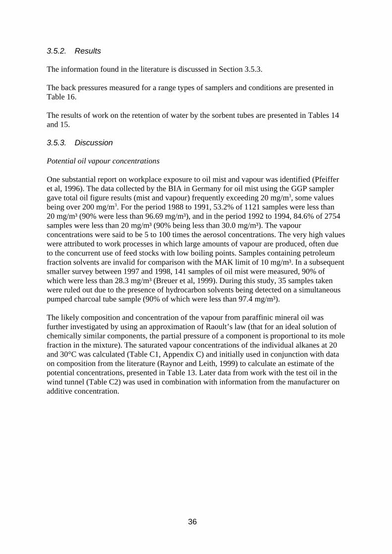
3.5.2. Results

The information found in the literature is discussed in Section 3.5.3.

The back pressures measured for a range types of samplers and conditions are presented in Table 16.

The results of work on the retention of water by the sorbent tubes are presented in Tables 14 and 15.

3.5.3. Discussion

Potential oil vapour concentrations

One substantial report on workplace exposure to oil mist and vapour was identified (Pfeiffer et al, 1996). The data collected by the BIA in Germany for oil mist using the GGP sampler gave total oil figure results (mist and vapour) frequently exceeding 20 mg/m3, some values being over 200 mg/m3. For the period 1988 to 1991, 53.2% of 1121 samples were less than 20 mg/m³ (90% were less than 96.69 mg/m³), and in the period 1992 to 1994, 84.6% of 2754 samples were less than 20 mg/m³ (90% being less than 30.0 mg/m³). The vapour concentrations were said to be 5 to 100 times the aerosol concentrations. The very high values were attributed to work processes in which large amounts of vapour are produced, often due to the concurrent use of feed stocks with low boiling points. Samples containing petroleum fraction solvents are invalid for comparison with the MAK limit of 10 mg/m³. In a subsequent smaller survey between 1997 and 1998, 141 samples of oil mist were measured, 90% of which were less than 28.3 mg/m³ (Breuer et al, 1999). During this study, 35 samples taken were ruled out due to the presence of hydrocarbon solvents being detected on a simultaneous pumped charcoal tube sample (90% of which were less than 97.4 mg/m³).

The likely composition and concentration of the vapour from paraffinic mineral oil was further investigated by using an approximation of Raoult’s law (that for an ideal solution of chemically similar components, the partial pressure of a component is proportional to its mole fraction in the mixture). The saturated vapour concentrations of the individual alkanes at 20 and 30°C was calculated (Table C1, Appendix C) and initially used in conjunction with data on composition from the literature (Raynor and Leith, 1999) to calculate an estimate of the potential concentrations, presented in Table 13. Later data from work with the test oil in the wind tunnel (Table C2) was used in combination with information from the manufacturer on additive concentration.

36

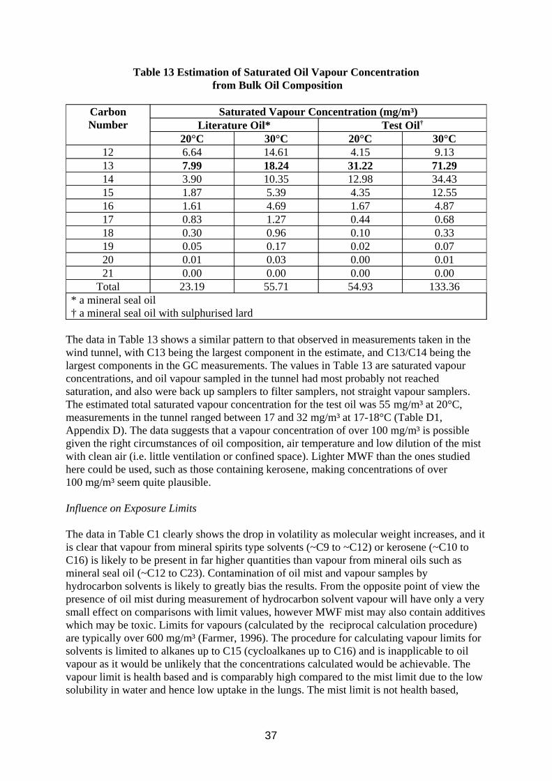
Table 13 Estimation of Saturated Oil Vapour Concentration from Bulk Oil Composition

Carbon Number

Saturated Vapour Concentration (mg/m³) Literature Oil* Test Oil†

20°C 30°C 20°C 30°C 12 6.64 14.61 4.15 9.13 13 7.99 18.24 31.22 71.29 14 3.90 10.35 12.98 34.43 15 1.87 5.39 4.35 12.55 16 1.61 4.69 1.67 4.87 17 0.83 1.27 0.44 0.68 18 0.30 0.96 0.10 0.33 19 0.05 0.17 0.02 0.07 20 0.01 0.03 0.00 0.01 21 0.00 0.00 0.00 0.00

Total 23.19 55.71 54.93 133.36 * a mineral seal oil † a mineral seal oil with sulphurised lard

The data in Table 13 shows a similar pattern to that observed in measurements taken in the wind tunnel, with C13 being the largest component in the estimate, and C13/C14 being the largest components in the GC measurements. The values in Table 13 are saturated vapour concentrations, and oil vapour sampled in the tunnel had most probably not reached saturation, and also were back up samplers to filter samplers, not straight vapour samplers. The estimated total saturated vapour concentration for the test oil was 55 mg/m³ at 20°C, measurements in the tunnel ranged between 17 and 32 mg/m³ at 17-18°C (Table D1, Appendix D). The data suggests that a vapour concentration of over 100 mg/m³ is possible given the right circumstances of oil composition, air temperature and low dilution of the mist with clean air (i.e. little ventilation or confined space). Lighter MWF than the ones studied here could be used, such as those containing kerosene, making concentrations of over 100 mg/m³ seem quite plausible.

Influence on Exposure Limits

The data in Table C1 clearly shows the drop in volatility as molecular weight increases, and it is clear that vapour from mineral spirits type solvents (~C9 to ~C12) or kerosene (~C10 to C16) is likely to be present in far higher quantities than vapour from mineral oils such as mineral seal oil (~C12 to C23). Contamination of oil mist and vapour samples by hydrocarbon solvents is likely to greatly bias the results. From the opposite point of view the presence of oil mist during measurement of hydrocarbon solvent vapour will have only a very small effect on comparisons with limit values, however MWF mist may also contain additives which may be toxic. Limits for vapours (calculated by the reciprocal calculation procedure) are typically over 600 mg/m³ (Farmer, 1996). The procedure for calculating vapour limits for solvents is limited to alkanes up to C15 (cycloalkanes up to C16) and is inapplicable to oil vapour as it would be unlikely that the concentrations calculated would be achievable. The vapour limit is health based and is comparably high compared to the mist limit due to the low solubility in water and hence low uptake in the lungs. The mist limit is not health based,

37

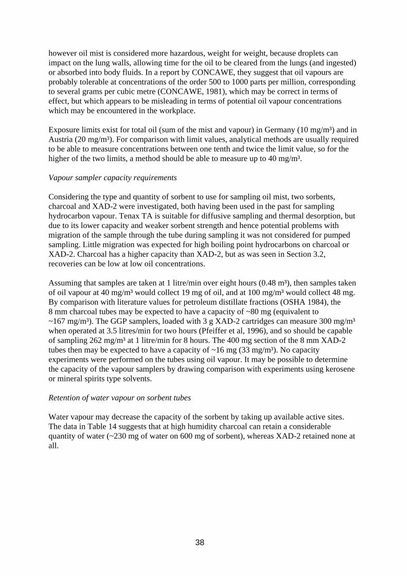
however oil mist is considered more hazardous, weight for weight, because droplets can impact on the lung walls, allowing time for the oil to be cleared from the lungs (and ingested) or absorbed into body fluids. In a report by CONCAWE, they suggest that oil vapours are probably tolerable at concentrations of the order 500 to 1000 parts per million, corresponding to several grams per cubic metre (CONCAWE, 1981), which may be correct in terms of effect, but which appears to be misleading in terms of potential oil vapour concentrations which may be encountered in the workplace.

Exposure limits exist for total oil (sum of the mist and vapour) in Germany (10 mg/m³) and in Austria (20 mg/m³). For comparison with limit values, analytical methods are usually required to be able to measure concentrations between one tenth and twice the limit value, so for the higher of the two limits, a method should be able to measure up to 40 mg/m³.

Vapour sampler capacity requirements

Considering the type and quantity of sorbent to use for sampling oil mist, two sorbents, charcoal and XAD-2 were investigated, both having been used in the past for sampling hydrocarbon vapour. Tenax TA is suitable for diffusive sampling and thermal desorption, but due to its lower capacity and weaker sorbent strength and hence potential problems with migration of the sample through the tube during sampling it was not considered for pumped sampling. Little migration was expected for high boiling point hydrocarbons on charcoal or XAD-2. Charcoal has a higher capacity than XAD-2, but as was seen in Section 3.2, recoveries can be low at low oil concentrations.

Assuming that samples are taken at 1 litre/min over eight hours (0.48 m³), then samples taken of oil vapour at 40 mg/m³ would collect 19 mg of oil, and at 100 mg/m³ would collect 48 mg. By comparison with literature values for petroleum distillate fractions (OSHA 1984), the 8 mm charcoal tubes may be expected to have a capacity of ~80 mg (equivalent to ~167 mg/m³). The GGP samplers, loaded with 3 g XAD-2 cartridges can measure 300 mg/m³ when operated at 3.5 litres/min for two hours (Pfeiffer et al, 1996), and so should be capable of sampling 262 mg/m³ at 1 litre/min for 8 hours. The 400 mg section of the 8 mm XAD-2 tubes then may be expected to have a capacity of ~16 mg (33 mg/m³). No capacity experiments were performed on the tubes using oil vapour. It may be possible to determine the capacity of the vapour samplers by drawing comparison with experiments using kerosene or mineral spirits type solvents.

Retention of water vapour on sorbent tubes

Water vapour may decrease the capacity of the sorbent by taking up available active sites. The data in Table 14 suggests that at high humidity charcoal can retain a considerable quantity of water (~230 mg of water on 600 mg of sorbent), whereas XAD-2 retained none at all.

38

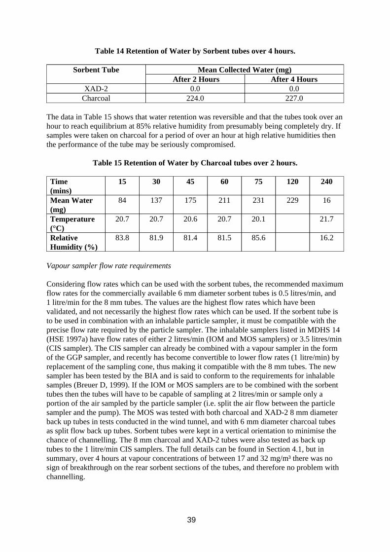
Table 14 Retention of Water by Sorbent tubes over 4 hours.

Sorbent Tube Mean Collected Water (mg) After 2 Hours After 4 Hours

XAD-2 0.0 0.0 Charcoal 224.0 227.0

The data in Table 15 shows that water retention was reversible and that the tubes took over an hour to reach equilibrium at 85% relative humidity from presumably being completely dry. If samples were taken on charcoal for a period of over an hour at high relative humidities then the performance of the tube may be seriously compromised.

Table 15 Retention of Water by Charcoal tubes over 2 hours.

Time (mins)

15 30 45 60 75 120 240

Mean Water (mg)

84 137 175 211 231 229 16

Temperature (°C)

20.7 20.7 20.6 20.7 20.1 21.7

Relative Humidity (%)

83.8 81.9 81.4 81.5 85.6 16.2

Vapour sampler flow rate requirements

Considering flow rates which can be used with the sorbent tubes, the recommended maximum flow rates for the commercially available 6 mm diameter sorbent tubes is 0.5 litres/min, and 1 litre/min for the 8 mm tubes. The values are the highest flow rates which have been validated, and not necessarily the highest flow rates which can be used. If the sorbent tube is to be used in combination with an inhalable particle sampler, it must be compatible with the precise flow rate required by the particle sampler. The inhalable samplers listed in MDHS 14 (HSE 1997a) have flow rates of either 2 litres/min (IOM and MOS samplers) or 3.5 litres/min (CIS sampler). The CIS sampler can already be combined with a vapour sampler in the form of the GGP sampler, and recently has become convertible to lower flow rates (1 litre/min) by replacement of the sampling cone, thus making it compatible with the 8 mm tubes. The new sampler has been tested by the BIA and is said to conform to the requirements for inhalable samples (Breuer D, 1999). If the IOM or MOS samplers are to be combined with the sorbent tubes then the tubes will have to be capable of sampling at 2 litres/min or sample only a portion of the air sampled by the particle sampler (i.e. split the air flow between the particle sampler and the pump). The MOS was tested with both charcoal and XAD-2 8 mm diameter back up tubes in tests conducted in the wind tunnel, and with 6 mm diameter charcoal tubes as split flow back up tubes. Sorbent tubes were kept in a vertical orientation to minimise the chance of channelling. The 8 mm charcoal and XAD-2 tubes were also tested as back up tubes to the 1 litre/min CIS samplers. The full details can be found in Section 4.1, but in summary, over 4 hours at vapour concentrations of between 17 and 32 mg/m³ there was no sign of breakthrough on the rear sorbent sections of the tubes, and therefore no problem with channelling.

39

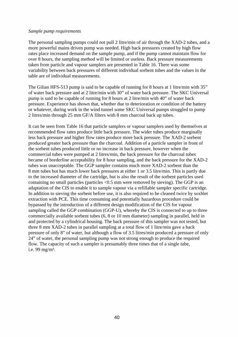
Sample pump requirements

The personal sampling pumps could not pull 2 litre/min of air through the XAD-2 tubes, and a more powerful mains driven pump was needed. High back pressures created by high flow rates place increased demand on the sample pump, and if the pump cannot maintain flow for over 8 hours, the sampling method will be limited or useless. Back pressure measurements taken from particle and vapour samplers are presented in Table 16. There was some variability between back pressures of different individual sorbent tubes and the values in the table are of individual measurements.

The Gilian HFS-513 pump is said to be capable of running for 8 hours at 1 litre/min with 35” of water back pressure and at 2 litre/min with 30” of water back pressure. The SKC Universal pump is said to be capable of running for 8 hours at 2 litre/min with 40” of water back pressure. Experience has shown that, whether due to deterioration or condition of the battery or whatever, during work in the wind tunnel some SKC Universal pumps struggled to pump 2 litres/min through 25 mm GF/A filters with 8 mm charcoal back up tubes.

It can be seen from Table 16 that particle samplers or vapour samplers used by themselves at recommended flow rates produce little back pressure. The wider tubes produce marginally less back pressure and higher flow rates produce more back pressure. The XAD-2 sorbent produced greater back pressure than the charcoal. Addition of a particle sampler in front of the sorbent tubes produced little or no increase in back pressure, however when the commercial tubes were pumped at 2 litres/min, the back pressure for the charcoal tubes became of borderline acceptability for 8 hour sampling, and the back pressure for the XAD-2 tubes was unacceptable. The GGP sampler contains much more XAD-2 sorbent than the 8 mm tubes but has much lower back pressures at either 1 or 3.5 litre/min. This is partly due to the increased diameter of the cartridge, but is also the result of the sorbent particles used containing no small particles (particles <0.5 mm were removed by sieving). The GGP is an adaptation of the CIS to enable it to sample vapour via a refillable sampler specific cartridge. In addition to sieving the sorbent before use, it is also required to be cleaned twice by soxhlet extraction with PCE. This time consuming and potentially hazardous procedure could be bypassed by the introduction of a different design modification of the CIS for vapour sampling called the GGP combination (GGP-U), whereby the CIS is connected to up to three commercially available sorbent tubes (6, 8 or 10 mm diameter) sampling in parallel, held in and protected by a cylindrical housing. The back pressure of this sampler was not tested, but three 8 mm XAD-2 tubes in parallel sampling at a total flow of 1 litre/min gave a back pressure of only 8” of water, but although a flow of 3.5 litres/min produced a pressure of only 24” of water, the personal sampling pump was not strong enough to produce the required flow. The capacity of such a sampler is presumably three times that of a single tube, i.e. 99 mg/m³.

40

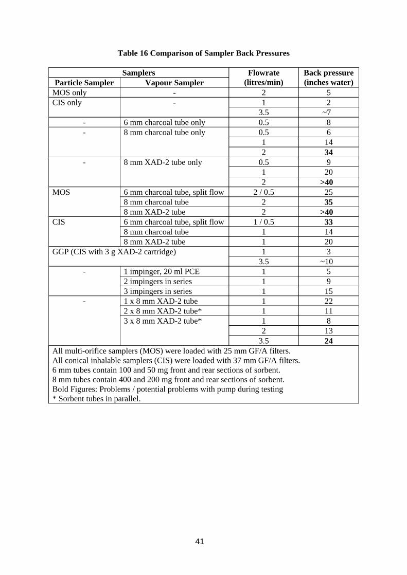
Table 16 Comparison of Sampler Back Pressures

Samplers Flowrate (litres/min)

Back pressure (inches water)Particle Sampler Vapour Sampler

MOS only - 2 5 CIS only - 1 2

3.5 ~7 - 6 mm charcoal tube only 0.5 8 - 8 mm charcoal tube only 0.5 6

1 14 2 34

- 8 mm XAD-2 tube only 0.5 9 1 20 2 >40

MOS 6 mm charcoal tube, split flow 2 / 0.5 25 8 mm charcoal tube 2 35 8 mm XAD-2 tube 2 >40

CIS 6 mm charcoal tube, split flow 1 / 0.5 33 8 mm charcoal tube 1 14 8 mm XAD-2 tube 1 20

GGP (CIS with 3 g XAD-2 cartridge) 1 3 3.5 ~10

- 1 impinger, 20 ml PCE 1 5 2 impingers in series 1 9 3 impingers in series 1 15

- 1 x 8 mm XAD-2 tube 1 22 2 x 8 mm XAD-2 tube* 1 11 3 x 8 mm XAD-2 tube* 1 8

2 13 3.5 24

All multi-orifice samplers (MOS) were loaded with 25 mm GF/A filters. All conical inhalable samplers (CIS) were loaded with 37 mm GF/A filters. 6 mm tubes contain 100 and 50 mg front and rear sections of sorbent. 8 mm tubes contain 400 and 200 mg front and rear sections of sorbent. Bold Figures: Problems / potential problems with pump during testing * Sorbent tubes in parallel.

41

3.5.4. Conclusion

w There is limited information available on occupational exposures to oil vapour, however guidance can be taken from exposure limits set for total airborne oil in Germany (10 mg/m³) and Austria (20 mg/m³).

w Oil vapour methods should be able to measure up to 40 mg/m³, however for more volatile fluids (e.g. background or added kerosene or mineral spirits) in conditions of high temperatures and with poor ventilation, concentrations of over 100 mg/m³ could be encountered.

w Oil vapour concentrations will be lower than those of hydrocarbon solvents, and any exposure limit calculated by the reciprocal method would be inappropriate.

w Charcoal and XAD-2 are suitable sorbents for sampling oil vapour. Charcoal has a higher capacity than XAD-2, however the capacity of XAD-2, unlike charcoal, should not be affected by high humidity during sampling. Both sorbents should be sufficiently strong for high boiling point hydrocarbons to not suffer from any significant migration.

w The 8 mm charcoal tube is estimated as capable of sampling up to 167 mg/m³ over 8 hours at 1 litre/min, the equivalent XAD-2 tube only 33 mg/m³. The GGP sampler packed with XAD-2 is said to be capable of measuring 300 mg/m³ over two hours (at 3.5 litres/min) and it follows that it should be capable of sampling 262 mg/m³ over 8 hours at 1 litre/min.

w A new sampler (GGP-U) combining the CIS with up to 3 commercially available 8 mm XAD-2 tubes would have an estimated capacity of 99 mg/m³ (over 8 hours at 1 litre/min). Such a sampler would not require lengthy and potentially hazardous preparation of sorbent by the analyst (as would be the case with the GGP sampler).

w No actual capacity measurements were made with oil vapour during this project. It should be possible to measure capacity by substituting the more easily vaporised kerosene during the measurement experiment.

w Alternatives to the GGP type combination sampler can be constructed by connecting existing inhalable samplers with 8 mm sorbent tubes. The CIS can be modified to sample at 1 litre/min making it compatible with the sorbent tubes’ recommended maximum flow rate. The MOS sampler can be combined with 8 mm charcoal tubes and operated at 2 litre/min. Care however should be taken that connections are secure and that tubing cannot be easily crimped.

w Flow rates of 2 litres/min can be used satisfactorily with 8 mm sorbent tubes. Tests at vapour concentrations of between 17 and 32 mg/m³ over 4 hours showed no sign of sample breakthrough. The back pressure required for charcoal tubes

42

could be quite demanding for many personal sampling pumps, and impossible XAD-2 tubes.

w It is possible to split the air flow behind the filter in two, one of which leads to a sorbent sampler, in order to lower the amount of vapour sample collected, however such a procedure would not be recommended. No commercially available unit is available and a self made device is likely to be relatively large and awkward to set up in the field.

43

3.6. Investigation of Sampling Total Airborne Oil by Lone Pumped Sorbent Tubes

The Industrial Hygiene subgroup of CONCAWE (the oil companies international study group for conservation of clean air and water- Europe) recognised the problem of sample loss from filters during collection of mist from low boiling range oils in their report on determination of oil mist (CONCAWE 1981), and suggested that vapour concentrations were more likely to be appropriate criteria for assessing exposure. No method is described but it is assumed that it infers sampling via a pumped sorbent tube. The common method for analysis of organic solvents is via sampling onto a 6 mm diameter charcoal tube, solvent desorption in CS2 and analysis by GC-FID. There are two potential problems with this approach. Firstly a lone sorbent tube will have different particle sampling characteristics compared to the inhalable samplers recommended in MDHS 14 (HSE 1997a), and as discussed in Section 3.3, it is possible that not all the components of the MWF sampled will volatilize and be detected when analysed by GC. This approach was investigated however, with a few modifications, to see how well it could reflect exposure to total airborne oil (mist and vapour) if it were used. The effect of different flow rates and charcoal tube sizes on sampling efficiency were studied, but the tubes were analysed by FTIR rather than GC-FID.

Although lone pumped tubes under sample particles, the fact that they do sample some particles would make them unsuitable for accurate estimation of oil vapour only concentrations. In atmospheres where the mist phase was negligible compared to the vapour phase the tubes should give good estimates of the vapour.

3.6.1. Method

The effect of flow rate was investigated by sampling oil mist and vapour in the wind tunnel using 8 mm charcoal tubes over a period of 4 hours. Three replicate tubes were taken each at 0.1 and 0.5 litre/min, and 6 replicates at 0.2 litre/min. The tubes were orientated downwards and flows were controlled via a critical orifice. None of the tubes were fitted with protective covers in case it affected sampling of the mist particles. Three reference samplers were run in parallel, the filter and impinger results being summed for comparison with the pumped sorbent tubes. The samples were stored in a refrigerator until analysis. The 0.1 litre/min samples were extracted in 5 ml PCE, the 0.2 litre/min in 10 ml PCE and the 0.5 litre/min in 20 ml PCE for over 24 hours. The glass wool plugs and the internal glass walls were included in the extraction so that impacted mist particles would not be excluded. The outside surfaces of the tubes were wiped with a PCE soaked tissue before extraction to prevent non-sampled oil from contaminating the extracts. The reference method filters were extracted in 10 ml PCE over night.

Three small (6 mm outside diameter) and three medium (8 mm outside diameter) sized charcoal tubes were compared in a test similar to the work on flow rates. An additional three 8 mm tubes were included which had the sealed ends broken at the widest extent to see the effect of lowering the entrance air velocity. All other tubes were conventionally broken open at approximately two thirds of the distance from the tip to the shoulder of the tube. Samples of all tube types were taken at 200 ml/min over a 4 hour period. Tubes were extracted as above in 10 ml PCE.

44

The tube and filter extracts and impinger samples were analysed by FTIR using the conditions in Table A2 in Appendix A, calibrating on the combined peak absorbencies at 2957 and 2927 cm-1. The sorbent tube and filter extracts were background subtracted using the mean of extracts from blank tubes and filters, and solvent blanks were used to background subtract the impinger samples. The tube extract results were corrected for desorption efficiency.

3.6.2. Results

The results are summarised in Table 17. The particle size characterisation results are included in Table D1 in Appendix D.

3.6.3. Discussion

In the NIOSH method for naphthas (NIOSH, 1994b), 6 mm diameter charcoal tubes are used at flow rates between 0.01 and 0.2 litres/min for a total sample size of between 0.5 and 8 mg. For hydrocarbon solvents such as these a typical maximum sampling volume would be 20 litres of a vapour at concentration 400 mg/m³. The OSHA method (OSHA 1984) recommends collecting 3 litres at 0.2 litres/min (i.e. over fifteen minutes) on 6 mm diameter charcoal tubes. Sampling times are short and flow rates low in order that the tubes are not overloaded by analyte, however it would be desirable to be able to measure a full 8 hour shift. Due to their high volatility, solvent vapour concentrations can be very high. Although lower concentrations may be expected for oil vapour, it is known that some formulations are based on kerosene, and that there is the possibility of the tube sampling other organic compounds or retaining water thus reducing the capacity of the charcoal. If samples are limited to an 8 mg loading as suggested by NIOSH then a 6 mm tube should be able to measure 80 mg/m³ over 8 hours at 0.2 litres/min. The 8 mg limit (8% of sorbent weight) is a recommended limit, presumably set at a level with a safety margin as OSHA have found the capacity of 100 mg of charcoal for a mineral spirits type solvent vapour to be ~20 mg. No work was included here on breakthrough volumes or the effects of humidity.

The 8 mm tubes contain 4 times the amount of charcoal as the 6 mm tubes and so have a larger capacity. They should also have different sampling characteristics to the 6 mm tubes. The sampling apertures of the 6 mm, 8 mm and sectioned (fully opened) 8 mm tubes are approximately 2, 3 and 6 mm in diameter respectively. For identical flow rates, the air velocity will decrease as the size of the aperture increases, and lower air velocities should favour better collection efficiency of larger particles. Increasing flow rates will increase the air velocity and although the collection efficiency for larger particles may decrease, the size of the sample will increase and consequently detection limits decrease.

The results presented in Table 17 indicate that for the conditions present in the wind tunnel, the lone sorbent tubes compared quite well to the reference samples. Flow rate had little effect and although tube type appears to show the expected trend, when the CVs are considered their significance is diminished somewhat.

45

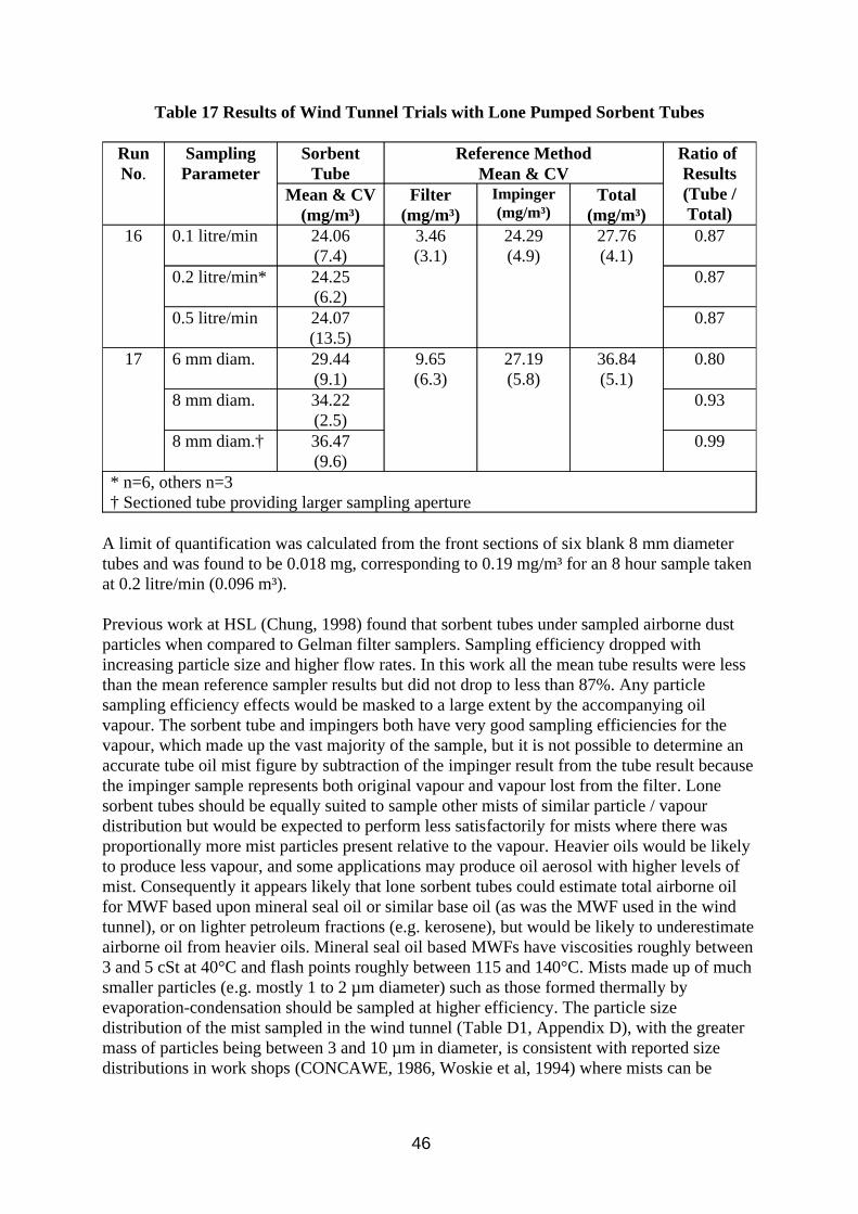
Table 17 Results of Wind Tunnel Trials with Lone Pumped Sorbent Tubes

Run No.

Sampling Parameter

Sorbent Tube

Reference Method Mean & CV

Ratio of Results (Tube / Total)

Mean & CV (mg/m³)

Filter (mg/m³)

Impinger (mg/m³)

Total (mg/m³)

16 0.1 litre/min 24.06 (7.4)

3.46 (3.1)

24.29 (4.9)

27.76 (4.1)

0.87

0.2 litre/min* 24.25 (6.2)

0.87

0.5 litre/min 24.07 (13.5)

0.87

17 6 mm diam. 29.44 (9.1)

9.65 (6.3)

27.19 (5.8)

36.84 (5.1)

0.80

8 mm diam. 34.22 (2.5)

0.93

8 mm diam.† 36.47 (9.6)

0.99

* n=6, others n=3 † Sectioned tube providing larger sampling aperture

A limit of quantification was calculated from the front sections of six blank 8 mm diameter tubes and was found to be 0.018 mg, corresponding to 0.19 mg/m³ for an 8 hour sample taken at 0.2 litre/min (0.096 m³).

Previous work at HSL (Chung, 1998) found that sorbent tubes under sampled airborne dust particles when compared to Gelman filter samplers. Sampling efficiency dropped with increasing particle size and higher flow rates. In this work all the mean tube results were less than the mean reference sampler results but did not drop to less than 87%. Any particle sampling efficiency effects would be masked to a large extent by the accompanying oil vapour. The sorbent tube and impingers both have very good sampling efficiencies for the vapour, which made up the vast majority of the sample, but it is not possible to determine an accurate tube oil mist figure by subtraction of the impinger result from the tube result because the impinger sample represents both original vapour and vapour lost from the filter. Lone sorbent tubes should be equally suited to sample other mists of similar particle / vapour distribution but would be expected to perform less satisfactorily for mists where there was proportionally more mist particles present relative to the vapour. Heavier oils would be likely to produce less vapour, and some applications may produce oil aerosol with higher levels of mist. Consequently it appears likely that lone sorbent tubes could estimate total airborne oil for MWF based upon mineral seal oil or similar base oil (as was the MWF used in the wind tunnel), or on lighter petroleum fractions (e.g. kerosene), but would be likely to underestimate airborne oil from heavier oils. Mineral seal oil based MWFs have viscosities roughly between 3 and 5 cSt at 40°C and flash points roughly between 115 and 140°C. Mists made up of much smaller particles (e.g. mostly 1 to 2 µm diameter) such as those formed thermally by evaporation-condensation should be sampled at higher efficiency. The particle size distribution of the mist sampled in the wind tunnel (Table D1, Appendix D), with the greater mass of particles being between 3 and 10 µm in diameter, is consistent with reported size distributions in work shops (CONCAWE, 1986, Woskie et al, 1994) where mists can be

46

formed thermally or mechanically. Further work would be required to identify the sampling methods true limitations. A more all encompassing method would be desirable but this method may provide a simple solution for the most problematical MWF types. If hydrocarbon solvents were present with the airborne oil then as with the pumped sorbent tubes used as back up tube to filters, the IR analytical method could not distinguish the solvent from the oil vapour.

3.6.4. Conclusion

w The use of lone pumped sorbent tubes to estimate airborne oil concentrations shows some promise for some types of MWF, but its use would be restricted and further evaluation is needed.

w The sorbent tube sampler is not ideal for sampling particles and is likely to seriously under sample larger particles, however if the aerosol contains a large proportion of vapour then the particle effects become less influential on the accuracy of the method.

w Lone pumped sorbent tubes may prove possible to sample mist and vapour from those MWF based upon kerosene, mineral seal oil or similar materials. It seems likely that they would be unsuitable to sample oil mist from heavier oils. Greater knowledge on likely vapour / mist concentrations of different types of oils is required, as well as sample breakthrough.

4. METHOD EVALUATION

4.1. Laboratory Work

The sampling methods described in Section 2.1 were tested using artificially generated oil mists created in a wind tunnel as described in Section 2.2.1. The experiments were primarily to compare the filter back-up methods for sampling and analysing the vapour, but they also allowed an opportunity for limited comparison of filter samplers, diffusive samplers and lone pumped sorbent tubes (the later two being described fully in Sections 3.4 and 3.5 respectively).

The reference method used a conical inhalable sampler (CIS) fitted with a 1 litre/min cone to sample the mist. Higher flow rates could not be used as they were incompatible with the midget impingers connected in line, thus excluding other inhalable samplers such as the multi-orifice sampler (MOS). The CIS sampler was consequently used as the particle sampler in many of the tests so that direct comparisons between vapour samplers could be made without any interference originating from possible differences in sampling characteristics or sample evaporation rates from the filter as may be the case if a different sampler was used. In addition to the impingers, the 8 mm diameter commercially available sorbent tubes also have a maximum recommended flow rate of 1 litre/min, although in this case it is thought that this restriction is the limit to which they have been validated and rather than one which is necessarily due to problems such as tube load capacity, safe sampling volumes or channelling within the sorbent. However increased back pressure caused by higher flow rates may be too large for sampling pumps to maintain flow for prolonged periods. Nevertheless CIS samplers

47

are thought relatively uncommon in the UK and it would be desirable to include some tests which used vapour samplers which were compatible with the MOS or IOM samplers. Although the GGP sampler is usually operated at higher flow rates for shorter periods (3.5 litres/min for 2 hours is recommended), it was used in this work with a 1 litre/min cone fitted in the CIS sampler portion of the assembly.

4.1.1. Method

Six samplers of the test method were tested next to three reference samplers for a period of 4 hours. The air temperature and humidity was measured before and after sampling, and the particle size distribution was measured during sampling.

A summary of the different combinations of filter samplers, vapour samplers, analytical methods and sorbent types tested can be found in Table D2 in Appendix D.

The reference method filters were immediately extracted in 10 ml PCE for over 1 hour and analysed by FTIR using the method in Table A2, calibrating on the combined peak absorbencies at 2957 and 2928 cm-1, and subtracting the mean response of three blank filter extracts. The reference method impingers (three in series) were analysed separately using the same method as the filters, subtracting the mean of the solvent blanks to compensate for additional hydrocarbon in the calibration standards. The volume of PCE remaining in the impingers after sampling was determined gravimetricaly.

Radiello tubes and charcoal back up tubes analysed by GC-FID were extracted in 2 ml CS2 and analysed by the method described in Section 3.3. Commercial 8 mm diameter charcoal and XAD back up tubes and GGP cartridges analysed by FTIR were extracted in 30 ml PCE and analysed by the method described in Section 3.2. Commercial 6 mm diameter charcoal back up tubes collected in the split flow apparatus were extracted in 10 ml PCE and analysed by FTIR by the method described in Section 3.2. Diffusive Tenax ATD tube and lone pumped sorbent tube analyses are described in Sections 3.4 and 3.6 respectively. In each case samples were stored in a refrigerator and when analysed were corrected for desorption efficiency and background material.

4.1.2. Results

A summary of the test conditions (temperature, relative humidity, particle size distribution and reference method results) are presented in Table D1, and of the test results in Table D2 in Appendix D.

4.1.3. Discussion

Artificial Oil Aerosol

The artificial oil mists formed in the wind tunnel were reasonably consistent in terms of particle size distribution but were more varied than anticipated in terms of levels of oil mist and vapour and total airborne oil. As discussed in Section 3.5.3, it is thought that the oil mist particle sizes produced were similar to those from actual oil mists formed mechanically. The principle reason for the variability of the oil concentrations measured was thought to be due

48

to variability in the rate the peristaltic pump supplied oil to the aerosol generator, caused partly by the oil leaching plasticisers from the tubing, and partly by inconsistent tautness of the tubing within the pump. The levels of oil mist and vapour attained were considered satisfactory, the total oil concentrations varied between 21 and 41 mg/m³ over 4 hours, equating to 10 to 20 mg/m³ as 8 hour time weighted averages. Oil mist levels varied between 3 and 10 mg/m³ (equating to 2 to 5 mg/m³ as 8 hour time weighted averages). Although there were no controls on air temperature or humidity due to the large volume of air travelling through the tunnel, and considering that it originated from outside the building, the atmospheric conditions were relatively stable during runs and between runs. Humidity was more varied than temperature but was never excessively wet.

Sample Integrity

The reference method impingers were effective at capturing the oil vapour. The first impinger of the series of three generally captured around 90% of the total sample, the third impinger contained less than 1% indicating good efficiency at sampling the vapour. Over the four hour sampling period the PCE in the first impinger steadily evaporated, reducing efficiency, but the second and third impingers trapped any oil vapour which remained in the air.

The commercially available sorbent tubes contain a front section of sorbent for sampling, and a rear section for checking for sample breakthrough. Over the 4 hours at the concentrations encountered none of the commercial tubes showed significant levels of oil on the rear sections. The NIOSH method for naphthas (NIOSH, 1994b), requires the back section to contain less than one tenth the amount of analyte found on the front to guard against sample loss. The rear sections of both the charcoal and XAD back up tubes collected in Run 12 and 14 respectively (both at 1 litre/min) all contained less than 1%, as did the charcoal tubes collected at 2 litre/min in run18. During the tests, two single samples were taken using XAD-2 back up tubes at 2 litres/min (runs 14 and 19) using a mains driven pump to sustain the air flow at a very high back pressure. The run 14 normalised result was 0.94, the rear section contained 1.5% of the front section, the run 19 normalised result was 0.89 and the rear section contained 2.6% of the front section, suggesting that although there was no serious breakthrough of oil, the test may have been approaching the limit of the tube capacity (~15 mg, or 3.8% of 400 mg). No oil was detected on the rear sections of the 6 mm tubes used for split sampling in run 19. There is no way of checking for breakthrough on the Radiello tubes or GGP samplers. The Radiello tubes being diffusive samplers it was assumed that the small quantities of analyte involved would not cause any problems. The GGP sampler, packed with 3 g of XAD-2, should be well within its capacity for oil vapour. It is said to be capable of sampling 126 mg of vapour (Pfeiffer et al, 1996) (4.2% of 3 g), and here only ~6 mg was collected. The BIA method requires that the XAD-2 used in the GGP sampler has less than 0.1 mg hydrocarbon per 3 g blank sample. The XAD-2 blank samples used here contained 0.048 mg (and the commercially available 8 mm diameter XAD-2 tubes contained 0.114 mg per 400 mg of sorbent).

All the samplers (with the exception of the Radiello tubes) collected sufficient analyte for the analytical methods to make acceptable measurements. The analytical method LOQs are listed in Table D3 in Appendix D for comparison. It should be pointed out that the test method LOQs are from a limited number of analyses of a limited number of blank sampling media, but generally it can be said that all the non-diffusive methods were quite sensitive and capable

49

of quantifying any significant oil vapour concentration. Methods are usually required to be capable of quantifying one tenth of a limit value; all the pumped methods here can quantify one tenth of 2 mg/m³. It can be seen that sampling at higher flow rates (e.g. 2 litre/min during runs 18 and 19) and thus collecting more sample lowers the LOQ, however other considerations such as sampler capacity and hardware limitations also appertain. The limitations of the diffusive methods were determined and more fully described in Section 3.4 The LOQ calculated for the lone charcoal tube analysis is quite low, especially when compared to the analysis of the charcoal back up tube analysed by FTIR. This figure (from a single analysis) however was calculated with no contribution from desorption efficiency. Charcoal has decreasing recovery at lower concentrations (Figure 7) and if recovery falls below 75% then the accuracy of the results would suffer. From the graph it can be estimated that the charcoal tube LOQ is still likely to be below 1 mg/m³ (for a 8 hour 0.2 litre/min sample), however at low concentrations XAD-2, which has high recoveries at low concentrations could be a more appropriate sorbent for sampling with lone tubes.

Comparison of Results

A summary of the results is presented in Table D2. The results have been normalised by dividing the mean test method result by the mean reference method result to facilitate comparison of the data. It can be seen that those methods using simple pumped sorbent back up tubes (run Nos 12, 13, 14 and 18) had good accuracy (all within 3% of the reference method), but those using the split system and the diffusive Radiello tube gave relatively low results. The Radiello tube underestimated the vapour concentration due to its poor uptake of significant heavier components. The most likely reasons for the low sample collected by the split systems are likely to be either an overestimate of the air flow through the sorbent tube (setting the flows on the split flow system was a relatively awkward and sensitive task) and/or loss of analyte by adsorption on the walls of the connecting tubing. The split flow system utilised a MOS sampler rather than the CIS type sampler used with the reference method. The smaller filter and higher flow rate used may have caused increased coalescence of droplets on the filter, reducing the sample surface area and slowing volatilisation. If this was the case then less vapour would have been available to the charcoal tube, and more oil would have been retained on the filter. TIP gravimetric filter measurements showed slightly lower concentrations from the MOS samplers than the CIS samplers (Table 18) as was also the case for the MOS and CIS filters from run 18, which showed good correlation between vapour measurements. It should be remembered from Section 3.1 however that measurement of volatile mist is subject to bias which may vary between filter sizes and loadings.

The two types of sampler used may not have exactly the same sampling characteristics, but statistically there is little difference between the weights of oil collected in runs 18 and 19. In the other runs the reference and test back up vapour samplers were both behind the CIS samplers.

50

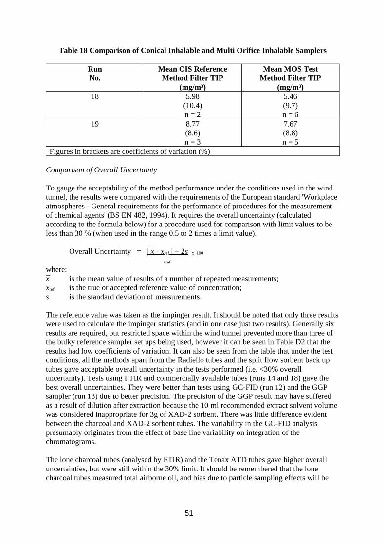
Table 18 Comparison of Conical Inhalable and Multi Orifice Inhalable Samplers

Run No.

Mean CIS Reference Method Filter TIP

(mg/m³)

Mean MOS Test Method Filter TIP

(mg/m³) 18 5.98

(10.4) n = 2

5.46 (9.7) n = 6

19 8.77 (8.6) n = 3

7.67 (8.8) n = 5

Figures in brackets are coefficients of variation (%)

Comparison of Overall Uncertainty

To gauge the acceptability of the method performance under the conditions used in the wind tunnel, the results were compared with the requirements of the European standard 'Workplace atmospheres - General requirements for the performance of procedures for the measurement of chemical agents' (BS EN 482, 1994). It requires the overall uncertainty (calculated according to the formula below) for a procedure used for comparison with limit values to be less than 30 % (when used in the range 0.5 to 2 times a limit value).

Overall Uncertainty = | x̄ - xref | + 2s x 100

xref

where: x̄ is the mean value of results of a number of repeated measurements; xref is the true or accepted reference value of concentration; s is the standard deviation of measurements.

The reference value was taken as the impinger result. It should be noted that only three results were used to calculate the impinger statistics (and in one case just two results). Generally six results are required, but restricted space within the wind tunnel prevented more than three of the bulky reference sampler set ups being used, however it can be seen in Table D2 that the results had low coefficients of variation. It can also be seen from the table that under the test conditions, all the methods apart from the Radiello tubes and the split flow sorbent back up tubes gave acceptable overall uncertainty in the tests performed (i.e. <30% overall uncertainty). Tests using FTIR and commercially available tubes (runs 14 and 18) gave the best overall uncertainties. They were better than tests using GC-FID (run 12) and the GGP sampler (run 13) due to better precision. The precision of the GGP result may have suffered as a result of dilution after extraction because the 10 ml recommended extract solvent volume was considered inappropriate for 3g of XAD-2 sorbent. There was little difference evident between the charcoal and XAD-2 sorbent tubes. The variability in the GC-FID analysis presumably originates from the effect of base line variability on integration of the chromatograms.

The lone charcoal tubes (analysed by FTIR) and the Tenax ATD tubes gave higher overall uncertainties, but were still within the 30% limit. It should be remembered that the lone charcoal tubes measured total airborne oil, and bias due to particle sampling effects will be

51

heavily dependant on the ratio of particles to vapour. The Tenax tube overall uncertainties were calculated using the impingers as reference method, however they were not measuring identical atmospheres because the impingers also sampled oil evaporated from the preceding filters, and both the bias and consequently the overall uncertainty are likely to be lower by a few percent. The data however needed correcting for oil vapour and mist collecting on the walls.

4.1.4. Conclusion

w All the vapour method measurements (with the exception of the Radiello tubes) have limits of quantification which show them to be capable of quantifying significant oil concentrations. They can quantify 8 hour samples as low as 0.2 mg/m³, and so could support a limit value as low as 2 mg/m³.

w The limit of quantification for total oil measured by lone pumped sorbent tube was calculated to be 0.2 mg/m³, however for charcoal this is likely to be higher due to lower recoveries at low concentrations, but is estimated to be less than 1 mg/m³.

w At the concentrations encountered in the wind tunnel, sorbent back up tubes give accurate results; tubes analysed by FTIR give greater precision than those analysed by GC-FID and there is little difference in accuracy or precision between results from charcoal or XAD-2 tubes.

w The Radiello diffusive back up sampler underestimates oil vapour concentration, due to low sensitivity to higher molecular weight components.

w The split flow sorbent back up tube design used underestimates oil vapour, possibly due to sample loss by adsorption on the internal walls of the sampler or due to less accurate flow rates.

w Under the test conditions the lone pumped sorbent tubes and the diffusive Tenax ATD tubes perform adequately. Under conditions of lower vapour and / or higher mist concentrations the accuracy of the lone tube could be expected to deteriorate due to its particle sampling characteristics. The Tenax ATD tube data needs correcting for oil vapour and mist collecting on the walls.

w Collection on sorbent back up tubes and analysis by FTIR give the most reliable results, having lowest overall uncertainty values.

4.2. Method Selection

Tables 19 to 21 summarise many of the outcomes of the work comparing analytical methods, sampler combinations and different sorbents. From this work the most suitable method for

52

measuring total oil would be sampling at 1 litre/min on a CIS sampler coupled to 8 mm XAD-2 sorbent tube(s), and analysis by FTIR. That is not to say that sampling on the more common MOS sampler at 2 litre/min with a 8 mm charcoal back up tube would be unsuitable, but the better protection of the filter from splashes, the lower sample pump back pressure and the higher desorption efficiency of XAD-2 make the CIS-XAD tube combination better. Either method could be recommended. Analysis by FTIR is favoured over GC because it can analyse both mist and vapour samples, and performs moderately better. Analysis by GC is more automated and so requires less staff time, however some of this time would be used up analysing the filter samples. The filters would presumably be analysed gravimetrically, which would suffer from requirements to reduce evaporative losses in storage and during equilibration. Both PCE and CS2 are toxic (50 ppm 8 hour TWA (time weighted average) occupational exposure standard and 10 ppm 8 hour TWA maximum exposure limit respectively), but CS2 is also highly volatile which affects sample solution concentration accuracy. Analysis by GC would not be affected by solvents like ethyl acetate however solvents such as white spirit would be detectable but not necessarily fully distinguishable from the oil. The two could be crudely differentiated by boiling point, but by either method, the presence of hydrocarbon solvents should be avoided.

53

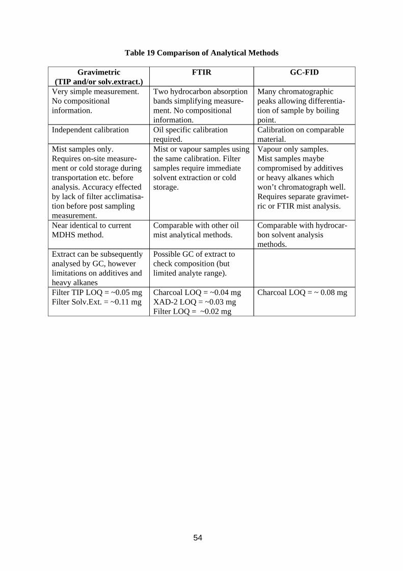
Table 19 Comparison of Analytical Methods

Gravimetric (TIP and/or solv.extract.)

FTIR GC-FID

Very simple measurement. No compositional information.

Two hydrocarbon absorption bands simplifying measure­ment. No compositional information.

Many chromatographic peaks allowing differentia­tion of sample by boiling point.

Independent calibration Oil specific calibration required.

Calibration on comparable material.

Mist samples only. Requires on-site measure­ment or cold storage during transportation etc. before analysis. Accuracy effected by lack of filter acclimatisa­tion before post sampling measurement.

Mist or vapour samples using the same calibration. Filter samples require immediate solvent extraction or cold storage.

Vapour only samples. Mist samples maybe compromised by additives or heavy alkanes which won’t chromatograph well. Requires separate gravimet­ric or FTIR mist analysis.

Near identical to current MDHS method.

Comparable with other oil mist analytical methods.

Comparable with hydrocar­bon solvent analysis methods.

Extract can be subsequently analysed by GC, however limitations on additives and heavy alkanes

Possible GC of extract to check composition (but limited analyte range).

Filter TIP LOQ = ~0.05 mg Filter Solv.Ext. = ~0.11 mg

Charcoal LOQ = ~0.04 mg XAD-2 LOQ = ~0.03 mg Filter LOQ = ~0.02 mg

Charcoal LOQ = ~ 0.08 mg

54

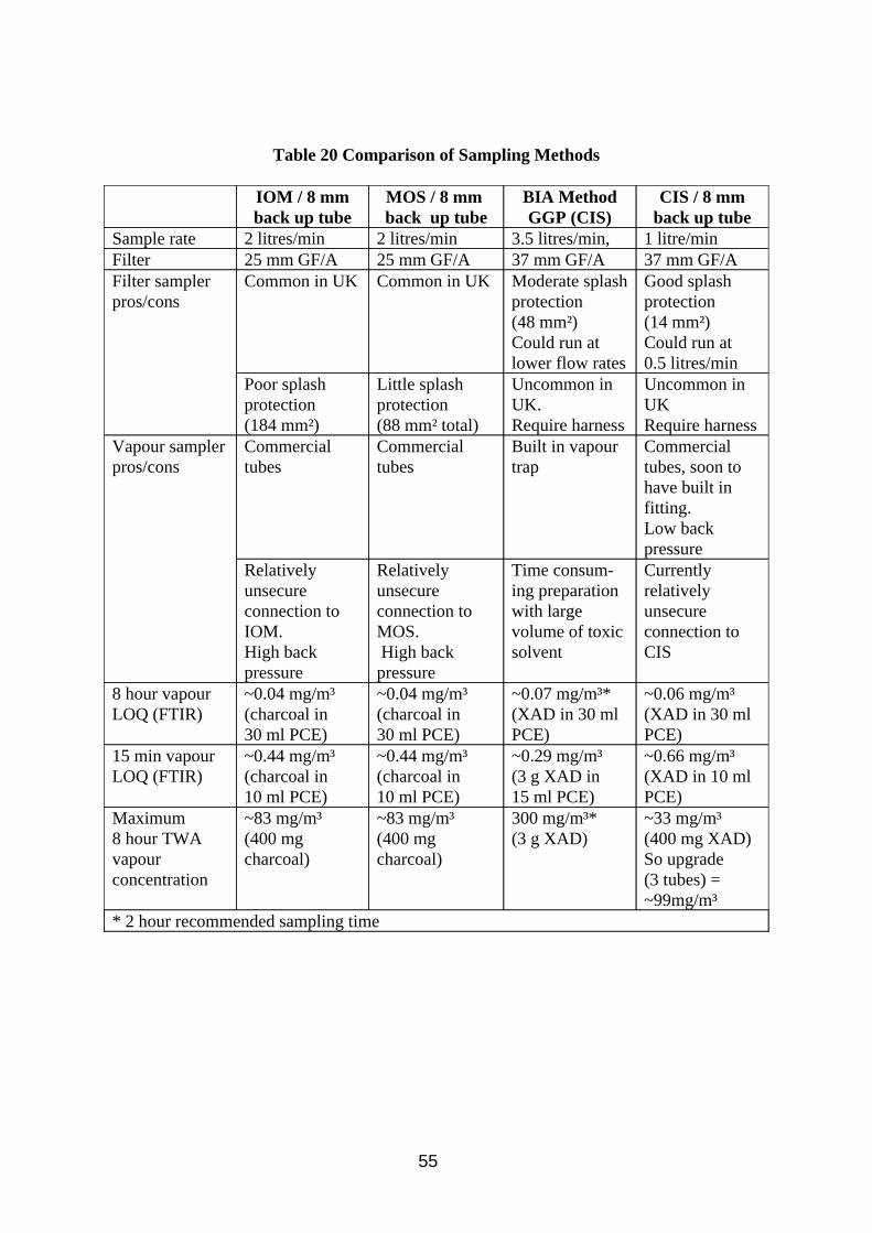
Table 20 Comparison of Sampling Methods

IOM / 8 mm MOS / 8 mm BIA Method CIS / 8 mm back up tube back up tube GGP (CIS) back up tube

Sample rate 2 litres/min 2 litres/min 3.5 litres/min, 1 litre/min Filter 25 mm GF/A 25 mm GF/A 37 mm GF/A 37 mm GF/A Filter sampler pros/cons

Common in UK Common in UK Moderate splash protection (48 mm²) Could run at

Good splash protection (14 mm²) Could run at

lower flow rates 0.5 litres/min Poor splash Little splash Uncommon in Uncommon in protection protection UK. UK (184 mm²) (88 mm² total) Require harness Require harness

Vapour sampler pros/cons

Commercial tubes

Commercial tubes

Built in vapour trap

Commercial tubes, soon to have built in fitting. Low back pressure

Relatively Relatively Time consum- Currently unsecure unsecure ing preparation relatively connection to connection to with large unsecure IOM. MOS. volume of toxic connection to High back High back solvent CIS pressure pressure

8 hour vapour ~0.04 mg/m³ ~0.04 mg/m³ ~0.07 mg/m³* ~0.06 mg/m³ LOQ (FTIR) (charcoal in (charcoal in (XAD in 30 ml (XAD in 30 ml

30 ml PCE) 30 ml PCE) PCE) PCE) 15 min vapour ~0.44 mg/m³ ~0.44 mg/m³ ~0.29 mg/m³ ~0.66 mg/m³ LOQ (FTIR) (charcoal in (charcoal in (3 g XAD in (XAD in 10 ml

10 ml PCE) 10 ml PCE) 15 ml PCE) PCE) Maximum ~83 mg/m³ ~83 mg/m³ 300 mg/m³* ~33 mg/m³ 8 hour TWA (400 mg (400 mg (3 g XAD) (400 mg XAD) vapour charcoal) charcoal) So upgrade concentration (3 tubes) =

~99mg/m³ * 2 hour recommended sampling time

55

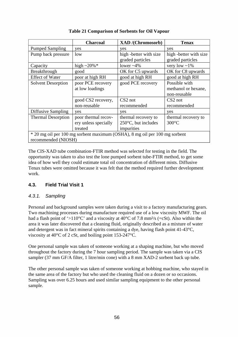
Table 21 Comparison of Sorbents for Oil Vapour

Charcoal XAD /(Chromosorb) Tenax Pumped Sampling yes yes yes Pump back pressure low high -better with size

graded particles high -better with size graded particles

Capacity high ~20%* lower ~4% very low ~1% Breakthrough good OK for C5 upwards OK for C8 upwards Effect of Water poor at high RH good at high RH good at high RH Solvent Desorption poor PCE recovery

at low loadings good PCE recovery Possible with

methanol or hexane, non-reusable

good CS2 recovery, non-reusable

CS2 not recommended

CS2 not recommended

Diffusive Sampling yes yes yes Thermal Desorption poor thermal recov­

ery unless specially treated

thermal recovery to 250°C, but includes impurities

thermal recovery to 300°C

* 20 mg oil per 100 mg sorbent maximum (OSHA), 8 mg oil per 100 mg sorbent recommended (NIOSH)

The CIS-XAD tube combination-FTIR method was selected for testing in the field. The opportunity was taken to also test the lone pumped sorbent tube-FTIR method, to get some idea of how well they could estimate total oil concentration of different mists. Diffusive Tenax tubes were omitted because it was felt that the method required further development work.

4.3. Field Trial Visit 1

4.3.1. Sampling

Personal and background samples were taken during a visit to a factory manufacturing gears. Two machining processes during manufacture required use of a low viscosity MWF. The oil had a flash point of ‘>110°C’ and a viscosity at 40°C of 7.8 mm²/s (=cSt). Also within the area it was later discovered that a cleaning fluid, originally described as a mixture of water and detergent was in fact mineral spirits containing a dye, having flash point 41-43°C, viscosity at 40°C of 2 cSt, and boiling point 153-247°C.

One personal sample was taken of someone working at a shaping machine, but who moved throughout the factory during the 7 hour sampling period. The sample was taken via a CIS sampler (37 mm GF/A filter, 1 litre/min cone) with a 8 mm XAD-2 sorbent back up tube.

The other personal sample was taken of someone working at hobbing machine, who stayed in the same area of the factory but who used the cleaning fluid on a dozen or so occasions. Sampling was over 6.25 hours and used similar sampling equipment to the other personal sample.

56

Three sets of static background samplers were positioned in the area around four working hobbing machines for periods of 4 hours. Air temperature and humidity during sampling were approximately 21°C and 35% respectively. Each set of background samplers (Figure 16) comprised two CIS samplers (37 mm GF/A filter, 1 litre/min cone) and one lone pumped 8 mm diameter charcoal tube (0.2 ml/min). One of the CIS samplers had a 8 mm XAD-2 sorbent back up tube, the other was connected to the reference method impingers. The impingers were connected to an L2SF sampling pump via a sorbent trap filled with charcoal.

After sampling the filters were immediately desorbed in 10 ml PCE, and the sorbent tubes sealed with plastic caps. Impinger samples were decanted into individual 30 ml bottles. Bulk samples of unused oil, used oil from the hobbing and shaping machines and of the cleaning solvent were taken.

57

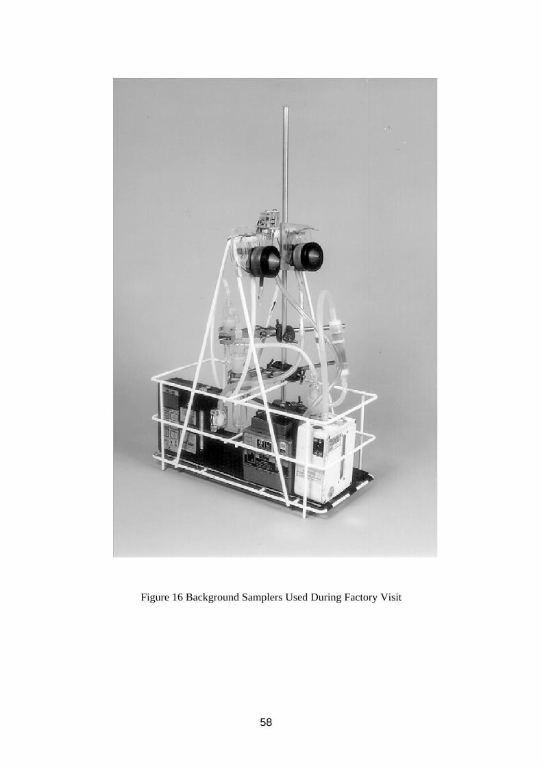
Figure 16 Background Samplers Used During Factory Visit

58

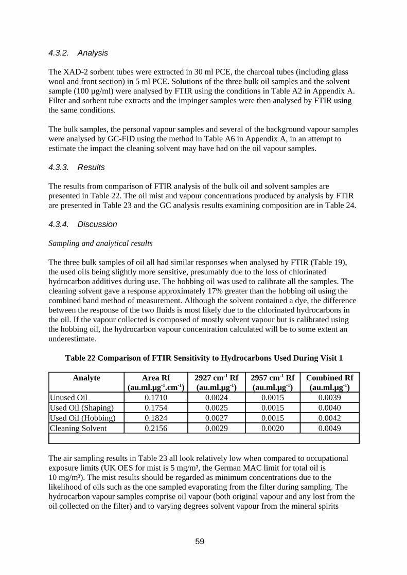
4.3.2. Analysis

The XAD-2 sorbent tubes were extracted in 30 ml PCE, the charcoal tubes (including glass wool and front section) in 5 ml PCE. Solutions of the three bulk oil samples and the solvent sample (100 µg/ml) were analysed by FTIR using the conditions in Table A2 in Appendix A. Filter and sorbent tube extracts and the impinger samples were then analysed by FTIR using the same conditions.

The bulk samples, the personal vapour samples and several of the background vapour samples were analysed by GC-FID using the method in Table A6 in Appendix A, in an attempt to estimate the impact the cleaning solvent may have had on the oil vapour samples.

4.3.3. Results

The results from comparison of FTIR analysis of the bulk oil and solvent samples are presented in Table 22. The oil mist and vapour concentrations produced by analysis by FTIR are presented in Table 23 and the GC analysis results examining composition are in Table 24.

4.3.4. Discussion

Sampling and analytical results

The three bulk samples of oil all had similar responses when analysed by FTIR (Table 19), the used oils being slightly more sensitive, presumably due to the loss of chlorinated hydrocarbon additives during use. The hobbing oil was used to calibrate all the samples. The cleaning solvent gave a response approximately 17% greater than the hobbing oil using the combined band method of measurement. Although the solvent contained a dye, the difference between the response of the two fluids is most likely due to the chlorinated hydrocarbons in the oil. If the vapour collected is composed of mostly solvent vapour but is calibrated using the hobbing oil, the hydrocarbon vapour concentration calculated will be to some extent an underestimate.

Table 22 Comparison of FTIR Sensitivity to Hydrocarbons Used During Visit 1

Analyte Area Rf (au.ml.µg-1.cm-1)

2927 cm-1 Rf (au.ml.µg-1)

2957 cm-1 Rf (au.ml.µg-1)

Combined Rf (au.ml.µg-1)

Unused Oil 0.1710 0.0024 0.0015 0.0039 Used Oil (Shaping) 0.1754 0.0025 0.0015 0.0040 Used Oil (Hobbing) 0.1824 0.0027 0.0015 0.0042 Cleaning Solvent 0.2156 0.0029 0.0020 0.0049

The air sampling results in Table 23 all look relatively low when compared to occupational exposure limits (UK OES for mist is 5 mg/m³, the German MAC limit for total oil is 10 mg/m³). The mist results should be regarded as minimum concentrations due to the likelihood of oils such as the one sampled evaporating from the filter during sampling. The hydrocarbon vapour samples comprise oil vapour (both original vapour and any lost from the oil collected on the filter) and to varying degrees solvent vapour from the mineral spirits

59

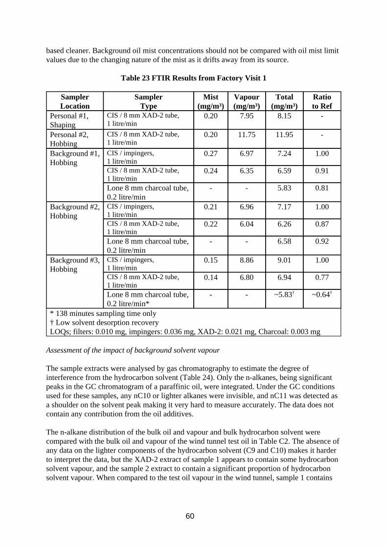
based cleaner. Background oil mist concentrations should not be compared with oil mist limit values due to the changing nature of the mist as it drifts away from its source.

Table 23 FTIR Results from Factory Visit 1

Sampler Location

Sampler Type

Mist (mg/m³)

Vapour (mg/m³)

Total (mg/m³)

Ratio to Ref

Personal #1, Shaping

CIS / 8 mm XAD-2 tube, 1 litre/min

0.20 7.95 8.15 -

Personal #2, Hobbing

CIS / 8 mm XAD-2 tube, 1 litre/min

0.20 11.75 11.95 -

Background #1, Hobbing

CIS / impingers, 1 litre/min

0.27 6.97 7.24 1.00

CIS / 8 mm XAD-2 tube, 1 litre/min

0.24 6.35 6.59 0.91

Lone 8 mm charcoal tube, 0.2 litre/min

- - 5.83 0.81

Background #2, Hobbing

CIS / impingers, 1 litre/min

0.21 6.96 7.17 1.00

CIS / 8 mm XAD-2 tube, 1 litre/min

0.22 6.04 6.26 0.87

Lone 8 mm charcoal tube, 0.2 litre/min

- - 6.58 0.92

Background #3, Hobbing

CIS / impingers, 1 litre/min

0.15 8.86 9.01 1.00

CIS / 8 mm XAD-2 tube, 1 litre/min

0.14 6.80 6.94 0.77

Lone 8 mm charcoal tube, 0.2 litre/min*

- - ~5.83† ~0.64†

* 138 minutes sampling time only † Low solvent desorption recovery LOQs; filters: 0.010 mg, impingers: 0.036 mg, XAD-2: 0.021 mg, Charcoal: 0.003 mg

Assessment of the impact of background solvent vapour

The sample extracts were analysed by gas chromatography to estimate the degree of interference from the hydrocarbon solvent (Table 24). Only the n-alkanes, being significant peaks in the GC chromatogram of a paraffinic oil, were integrated. Under the GC conditions used for these samples, any nC10 or lighter alkanes were invisible, and nC11 was detected as a shoulder on the solvent peak making it very hard to measure accurately. The data does not contain any contribution from the oil additives.

The n-alkane distribution of the bulk oil and vapour and bulk hydrocarbon solvent were compared with the bulk oil and vapour of the wind tunnel test oil in Table C2. The absence of any data on the lighter components of the hydrocarbon solvent (C9 and C10) makes it harder to interpret the data, but the XAD-2 extract of sample 1 appears to contain some hydrocarbon solvent vapour, and the sample 2 extract to contain a significant proportion of hydrocarbon solvent vapour. When compared to the test oil vapour in the wind tunnel, sample 1 contains

60

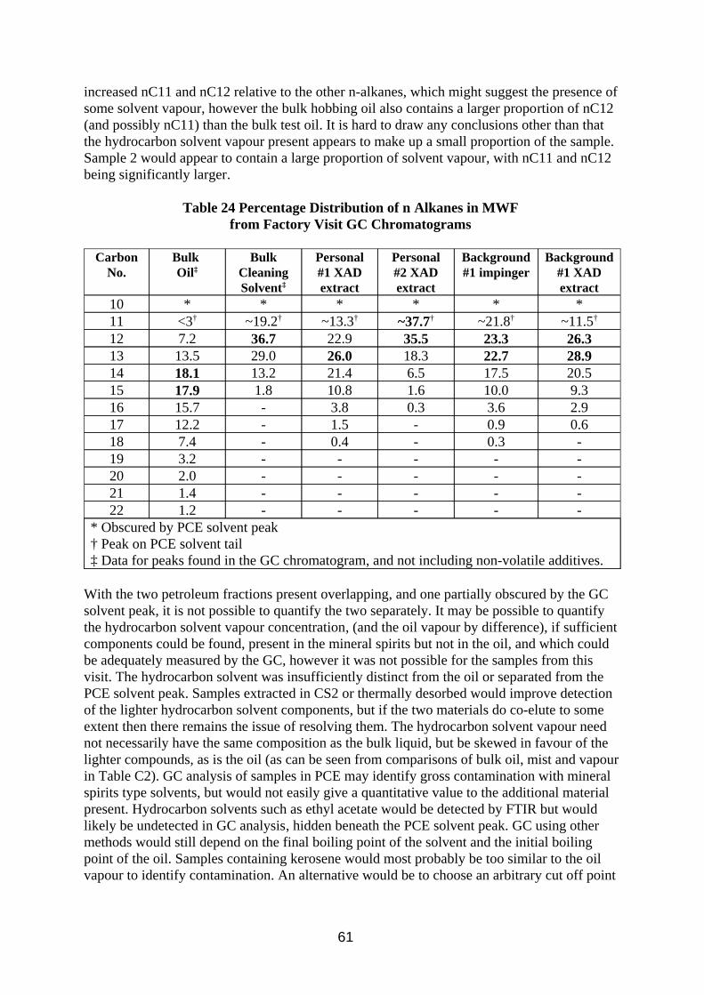
increased nC11 and nC12 relative to the other n-alkanes, which might suggest the presence of some solvent vapour, however the bulk hobbing oil also contains a larger proportion of nC12 (and possibly nC11) than the bulk test oil. It is hard to draw any conclusions other than that the hydrocarbon solvent vapour present appears to make up a small proportion of the sample. Sample 2 would appear to contain a large proportion of solvent vapour, with nC11 and nC12 being significantly larger.

Table 24 Percentage Distribution of n Alkanes in MWF from Factory Visit GC Chromatograms

Carbon No.

Bulk Oil‡

Bulk Cleaning Solvent‡

Personal #1 XAD extract

Personal #2 XAD extract

Background #1 impinger

Background #1 XAD extract

10 * * * * * * 11 <3† ~19.2† ~13.3† ~37.7† ~21.8† ~11.5†

12 7.2 36.7 22.9 35.5 23.3 26.3 13 13.5 29.0 26.0 18.3 22.7 28.9 14 18.1 13.2 21.4 6.5 17.5 20.5 15 17.9 1.8 10.8 1.6 10.0 9.3 16 15.7 - 3.8 0.3 3.6 2.9 17 12.2 - 1.5 - 0.9 0.6 18 7.4 - 0.4 - 0.3 -19 3.2 - - - - -20 2.0 - - - - -21 1.4 - - - - -22 1.2 - - - - -

* Obscured by PCE solvent peak † Peak on PCE solvent tail ‡ Data for peaks found in the GC chromatogram, and not including non-volatile additives.

With the two petroleum fractions present overlapping, and one partially obscured by the GC solvent peak, it is not possible to quantify the two separately. It may be possible to quantify the hydrocarbon solvent vapour concentration, (and the oil vapour by difference), if sufficient components could be found, present in the mineral spirits but not in the oil, and which could be adequately measured by the GC, however it was not possible for the samples from this visit. The hydrocarbon solvent was insufficiently distinct from the oil or separated from the PCE solvent peak. Samples extracted in CS2 or thermally desorbed would improve detection of the lighter hydrocarbon solvent components, but if the two materials do co-elute to some extent then there remains the issue of resolving them. The hydrocarbon solvent vapour need not necessarily have the same composition as the bulk liquid, but be skewed in favour of the lighter compounds, as is the oil (as can be seen from comparisons of bulk oil, mist and vapour in Table C2). GC analysis of samples in PCE may identify gross contamination with mineral spirits type solvents, but would not easily give a quantitative value to the additional material present. Hydrocarbon solvents such as ethyl acetate would be detected by FTIR but would likely be undetected in GC analysis, hidden beneath the PCE solvent peak. GC using other methods would still depend on the final boiling point of the solvent and the initial boiling point of the oil. Samples containing kerosene would most probably be too similar to the oil vapour to identify contamination. An alternative would be to choose an arbitrary cut off point

61

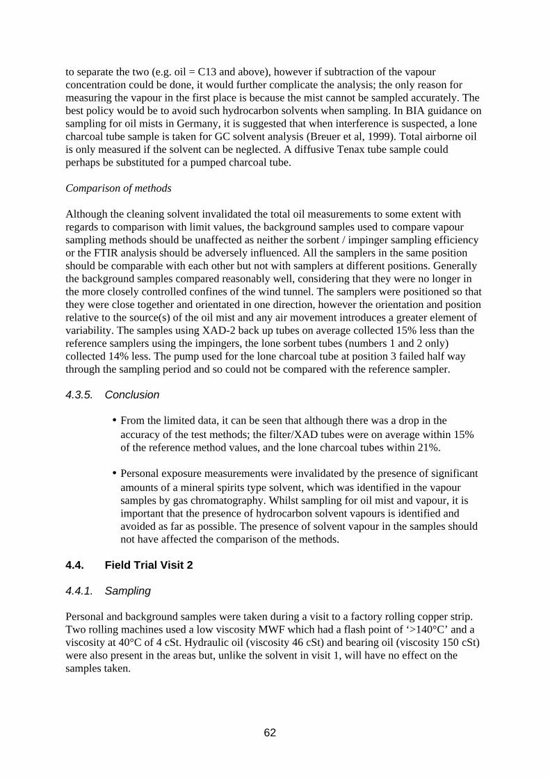
to separate the two (e.g. oil = C13 and above), however if subtraction of the vapour concentration could be done, it would further complicate the analysis; the only reason for measuring the vapour in the first place is because the mist cannot be sampled accurately. The best policy would be to avoid such hydrocarbon solvents when sampling. In BIA guidance on sampling for oil mists in Germany, it is suggested that when interference is suspected, a lone charcoal tube sample is taken for GC solvent analysis (Breuer et al, 1999). Total airborne oil is only measured if the solvent can be neglected. A diffusive Tenax tube sample could perhaps be substituted for a pumped charcoal tube.

Comparison of methods

Although the cleaning solvent invalidated the total oil measurements to some extent with regards to comparison with limit values, the background samples used to compare vapour sampling methods should be unaffected as neither the sorbent / impinger sampling efficiency or the FTIR analysis should be adversely influenced. All the samplers in the same position should be comparable with each other but not with samplers at different positions. Generally the background samples compared reasonably well, considering that they were no longer in the more closely controlled confines of the wind tunnel. The samplers were positioned so that they were close together and orientated in one direction, however the orientation and position relative to the source(s) of the oil mist and any air movement introduces a greater element of variability. The samples using XAD-2 back up tubes on average collected 15% less than the reference samplers using the impingers, the lone sorbent tubes (numbers 1 and 2 only) collected 14% less. The pump used for the lone charcoal tube at position 3 failed half way through the sampling period and so could not be compared with the reference sampler.

4.3.5. Conclusion

w From the limited data, it can be seen that although there was a drop in the accuracy of the test methods; the filter/XAD tubes were on average within 15% of the reference method values, and the lone charcoal tubes within 21%.

w Personal exposure measurements were invalidated by the presence of significant amounts of a mineral spirits type solvent, which was identified in the vapour samples by gas chromatography. Whilst sampling for oil mist and vapour, it is important that the presence of hydrocarbon solvent vapours is identified and avoided as far as possible. The presence of solvent vapour in the samples should not have affected the comparison of the methods.

4.4. Field Trial Visit 2

4.4.1. Sampling

Personal and background samples were taken during a visit to a factory rolling copper strip. Two rolling machines used a low viscosity MWF which had a flash point of ‘>140°C’ and a viscosity at 40°C of 4 cSt. Hydraulic oil (viscosity 46 cSt) and bearing oil (viscosity 150 cSt) were also present in the areas but, unlike the solvent in visit 1, will have no effect on the samples taken.

62

Personal samples were taken via CIS samplers (37 mm GF/A filter, 1 litre/min cone) with 8 mm XAD-2 sorbent back up tubes over ~6 hours. Two personal samples were taken of people working at a Schmitz MDS rolling machine, and one personal sample of someone working at a Frohling rolling machine. The MDS machine formed much visible mist which was mostly captured by an extract system. However behind the machine three sets of static background samplers were positioned in an area where some mist escaped. The static samplers were identical to those used in visit 1 (Section 4.3.1) and sampled for periods of 4 hours. Air temperature and relative humidity during sampling was 23-24°C and 56-63% respectively.

After sampling the filters were immediately desorbed in 10 ml PCE, and the sorbent tubes sealed with plastic caps. Impinger samples were decanted into individual 30 ml bottles. Bulk samples of unused and used oil were taken.

4.4.2. Analysis

Air and bulk samples were analysed as per Section 4.3.2, with the exception that there was no GC analysis.

4.4.3. Results

The results from comparison of FTIR analysis of the bulk oil and solvent samples are presented in Table 25. The oil mist and vapour concentrations produced by analysis by FTIR are presented in Table 26.

4.4.4. Discussion

Sampling and analytical results

The comments arising from sampling was more or less similar to those found in visit 1. Rucksack style harnesses were used to mount the personal samplers on visit 2, and these were found to be more satisfactory than the more traditional ‘Sam Browne’ style belts used in visit 1. The higher air temperatures encountered on the second visit resulted in more PCE evaporation from the impingers, however capture efficiency was not affected.

The three bulk samples of oil all had similar responses when analysed by FTIR (Table 25). The used MDS oil was used to calibrate all the samples. No other hydrocarbon solvents were used in the vicinity of sampling, however the person sampled operating the Frohling machine was a smoker, and the filter sample collected was clearly different from the others, being a deep yellow colour. Cigarette smoke contains hydrocarbons which will to some extent, be detected by FTIR.

63

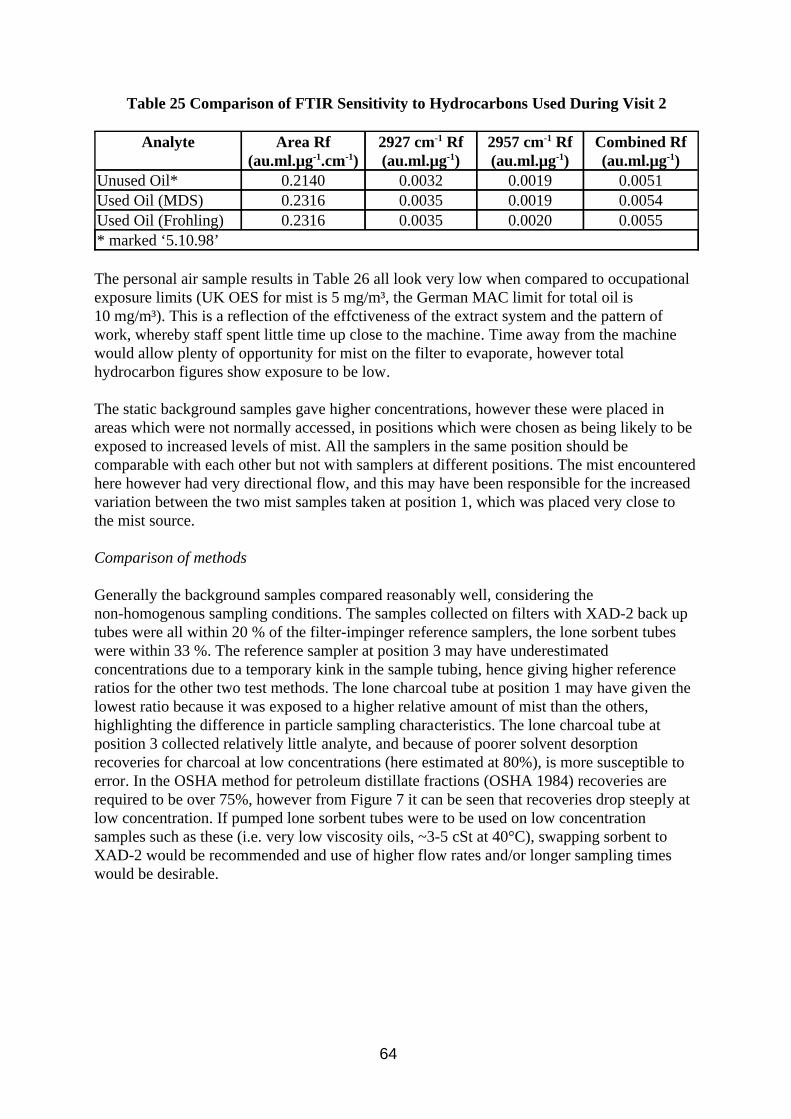
Table 25 Comparison of FTIR Sensitivity to Hydrocarbons Used During Visit 2

Analyte Area Rf (au.ml.µg-1.cm-1)

2927 cm-1 Rf (au.ml.µg-1)

2957 cm-1 Rf (au.ml.µg-1)

Combined Rf (au.ml.µg-1)

Unused Oil* 0.2140 0.0032 0.0019 0.0051 Used Oil (MDS) 0.2316 0.0035 0.0019 0.0054 Used Oil (Frohling) 0.2316 0.0035 0.0020 0.0055 * marked ‘5.10.98’

The personal air sample results in Table 26 all look very low when compared to occupational exposure limits (UK OES for mist is 5 mg/m³, the German MAC limit for total oil is 10 mg/m³). This is a reflection of the effctiveness of the extract system and the pattern of work, whereby staff spent little time up close to the machine. Time away from the machine would allow plenty of opportunity for mist on the filter to evaporate, however total hydrocarbon figures show exposure to be low.

The static background samples gave higher concentrations, however these were placed in areas which were not normally accessed, in positions which were chosen as being likely to be exposed to increased levels of mist. All the samplers in the same position should be comparable with each other but not with samplers at different positions. The mist encountered here however had very directional flow, and this may have been responsible for the increased variation between the two mist samples taken at position 1, which was placed very close to the mist source.

Comparison of methods

Generally the background samples compared reasonably well, considering the non-homogenous sampling conditions. The samples collected on filters with XAD-2 back up tubes were all within 20 % of the filter-impinger reference samplers, the lone sorbent tubes were within 33 %. The reference sampler at position 3 may have underestimated concentrations due to a temporary kink in the sample tubing, hence giving higher reference ratios for the other two test methods. The lone charcoal tube at position 1 may have given the lowest ratio because it was exposed to a higher relative amount of mist than the others, highlighting the difference in particle sampling characteristics. The lone charcoal tube at position 3 collected relatively little analyte, and because of poorer solvent desorption recoveries for charcoal at low concentrations (here estimated at 80%), is more susceptible to error. In the OSHA method for petroleum distillate fractions (OSHA 1984) recoveries are required to be over 75%, however from Figure 7 it can be seen that recoveries drop steeply at low concentration. If pumped lone sorbent tubes were to be used on low concentration samples such as these (i.e. very low viscosity oils, ~3-5 cSt at 40°C), swapping sorbent to XAD-2 would be recommended and use of higher flow rates and/or longer sampling times would be desirable.

64

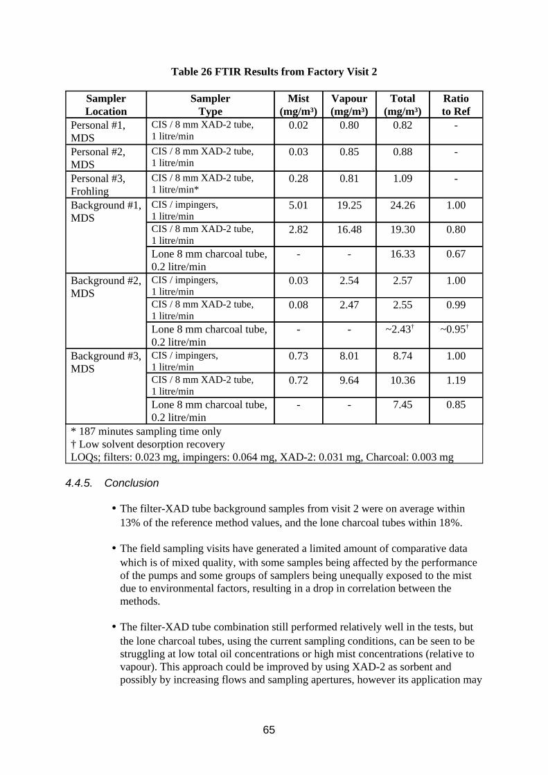
Table 26 FTIR Results from Factory Visit 2

Sampler Location

Sampler Type

Mist (mg/m³)

Vapour (mg/m³)

Total (mg/m³)

Ratio to Ref

Personal #1, MDS

CIS / 8 mm XAD-2 tube, 1 litre/min

0.02 0.80 0.82 -

Personal #2, MDS

CIS / 8 mm XAD-2 tube, 1 litre/min

0.03 0.85 0.88 -

Personal #3, Frohling

CIS / 8 mm XAD-2 tube, 1 litre/min*

0.28 0.81 1.09 -

Background #1, MDS

CIS / impingers, 1 litre/min

5.01 19.25 24.26 1.00

CIS / 8 mm XAD-2 tube, 1 litre/min

2.82 16.48 19.30 0.80

Lone 8 mm charcoal tube, 0.2 litre/min

- - 16.33 0.67

Background #2, MDS

CIS / impingers, 1 litre/min

0.03 2.54 2.57 1.00

CIS / 8 mm XAD-2 tube, 1 litre/min

0.08 2.47 2.55 0.99

Lone 8 mm charcoal tube, 0.2 litre/min

- - ~2.43† ~0.95†

Background #3, MDS

CIS / impingers, 1 litre/min

0.73 8.01 8.74 1.00

CIS / 8 mm XAD-2 tube, 1 litre/min

0.72 9.64 10.36 1.19

Lone 8 mm charcoal tube, 0.2 litre/min

- - 7.45 0.85

* 187 minutes sampling time only † Low solvent desorption recovery LOQs; filters: 0.023 mg, impingers: 0.064 mg, XAD-2: 0.031 mg, Charcoal: 0.003 mg

4.4.5. Conclusion

w The filter-XAD tube background samples from visit 2 were on average within 13% of the reference method values, and the lone charcoal tubes within 18%.

w The field sampling visits have generated a limited amount of comparative data which is of mixed quality, with some samples being affected by the performance of the pumps and some groups of samplers being unequally exposed to the mist due to environmental factors, resulting in a drop in correlation between the methods.

w The filter-XAD tube combination still performed relatively well in the tests, but the lone charcoal tubes, using the current sampling conditions, can be seen to be struggling at low total oil concentrations or high mist concentrations (relative to vapour). This approach could be improved by using XAD-2 as sorbent and possibly by increasing flows and sampling apertures, however its application may

65

be limited to the lowest viscosity oils, and not be applicable to other ‘volatile’ oils.

w Experience of interferents was gained during the factory visits. Hydrocarbon solvent vapour present in the workplace air will invalidate oil vapour samples.

5. REFERENCES

Breuer D (1999) ‘Measurement of Vapour-Aersol Mixtures’ J. Environ. Monit., 1, 299-305

Breuer D, Pfeiffer W, Berges M, Hennig M, Lichtenstein N, Pflaumbaum W and Stockmann R (1999) ‘BIA Report 5/99 Messen, Beurteilen un Schutzmassnahmen beim Umgang mit komplexen kohlenwasserstoffhaltigen Gemischen’ (Measurement, evaluation and safety measures in the handling of complex hydrocarbon containing mixtures) BIA, Sankt Augustin, Germany ISBN 3 88383 549 8 (available from HSE Translation Services, HSE Transl. No.: 16243)

BS EN 482 (1994) 'Workplace atmospheres - General requirements for the performance of procedures for the measurement of chemical agents' British Standards Institution ISBN 0 580 23644 7

Chung K Y K (1998) ‘Collection Efficiencies of Sorbing Tubes for Larger Particles’ Health and Safety Laboratory Aerosol Section. Internal report IR/A/98/06

CONCAWE (1981) 'Guidelines for the Determination of Atmospheric Concentrations of Oil Mists' Report no. 1/81. CONCAWE, Madouplein 1, B-1030, Brussel, Belgium

CONCAWE (1986) 'Health Aspects of Worker Exposure to Oil Mists' Report no. 86/69. CONCAWE, Madouplein 1, B-1030, Brussel, Belgium

Farmer T H (1996) ‘Occupational Hygiene Limits for Hydrocarbon Solvents’ Ann. occup. Hyg., 40, 237-242

HSE (1990) Methods for the Determination of Hazardous Substances MDHS 3 'Generation of test atmospheres of organic vapours by the syringe injection technique.' HSE Books ISBN 0 7176 0228 1

HSE (1994)

66

Methods for the Determination of Hazardous Substances MDHS 66 ‘Mixed Hydrocarbons (C5 to C10) in air’ HSE Books ISBN 0-7176-0867-0

HSE (1997a) Methods for the Determination of Hazardous Substances MDHS 14 ‘General methods for sampling and gravimetric analysis of respirable and total inhalable dust’ HSE Books ISBN 0 7176 1295 3

HSE (1997b) Methods for the Determination of Hazardous Substances MDHS 84 ‘Measurement of oil mist from mineral oil based metalworking fluids’ HSE Books ISBN 0 7176 1382 8

HSE (2000) Methods for the Determination of Hazardous Substances MDHS 96 ‘Volatile organic compounds in air (4) Laboratory method using pumped solid sorbent tubes, solvent desorption and gas chromatography’ HSE Books ISBN 0-7176-1756-4

Leith D, Leith F A and Boundby M G (1996) ‘Laboratory measurements of oil mist concentrations using filters and an electrostatic precipitator’ Am.Ind.Hyg.Assoc.J., 57, 1137-1141

Lichtenstein N, Hennig M, Friedrich J, Auffarth J, Hebisch R, Rentel K-H, Fricke H H, Möcklinghoff K and Dahmann D (1997) ‘Methods for Determining Exposure to Lacquer Aerosols and Solvent Vapours During Spray Painting’ Gefahrstoffe - Reinhaltung der Luft, 57, 39-45

NIOSH (1994a) Method 5026 ‘Mineral Oil Mist’ Manual of Analytical Methods, 4th Ed. National Institute of Occupational Safety and Health, Cincinnati, Ohio, USA

NIOSH (1994b) Method 1550 ‘Naphthas’ Manual of Analytical Methods, 4th Ed. National Institute of Occupational Safety and Health, Cincinnati, Ohio, USA

OSHA (1984) Method No. 48: ‘Petroleum Distillate Fractions (PDF)’ Analytical Methods Manual 1985, ISBN 0 936712 66 X OSHA Analytical Laboratory, Salt Lake City, Utah, USA

Pfeiffer W, Breuer D, Blome H, Deininger C, Hahn J, Kleine H, Nies E, Pflaumbaum W, Stockmann R, Willert G, and Sonnenschein G (1996)

67

‘BIA Report 7/96 Kuhlschmierstoffe’ (Cooling Lubricants) BIA, Sankt Augustin, Germany (available from HSE Translation Services, HSE Transl. No.: 97/17)

Raynor P C and Leith D (1999) ‘Evaporation of Accumulated Multicomponent Liquids from Fibrous Filters’ Ann. occup. Hyg., 43, 181-192

Simpson A T (1995) ‘Evaluation of Methods for Sampling and Analysis of Mineral Oil Metal Working Fluid Airborne Aerosol’ Health and Safety Laboratory Complex Substances and Fume Section. Internal report IR/L/SP/95/04

Simpson A T (1997) ‘Measurement of Volatile Metal Working Fluid Aerosol - Pilot Study’ Health and Safety Laboratory Complex Substances and Fume Section. Internal Report IR/L/SP/97/10

Unwin J, Dabill D, Simpson A, Groves J and Keen C (1997) 'On Site Measurement of Exposure to Chemicals' Health and Safety Laboratory Complex Substances and Fume Section. Internal report IR/L/SP/97/11

Volckens J, Boundy M, Leith D and Hands D (1999) ‘Oil Mist Concentration: A Comparison of Sampling Methods’ Am.Ind.Hyg.Assoc.J., 60, 684-689

Woskie S R, Smith T J, Hallock M F, Hammond S K, Rosenthal F, Eisen E A, Kriebal D and Greaves I A (1994) ‘Size Selective Pulmonary Dose Indices for Meatl-Working Fluid Aerosols in Machining and Grinding Operations in the Automobile Manufacturing Industry’ Am.Ind.Hyg.Assoc.J., 55, 20-29

Xiong J Q, Fang C and Cohen B S (1998) ‘A Portable Vapour Particle Sampler’ Am.Ind.Hyg.Assoc.J., 59, 614-621

68

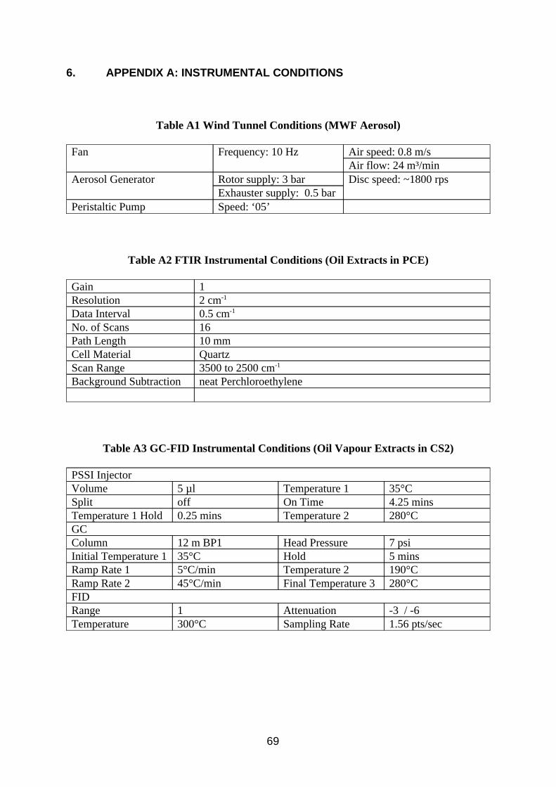
6. APPENDIX A: INSTRUMENTAL CONDITIONS

Table A1 Wind Tunnel Conditions (MWF Aerosol)

Fan Frequency: 10 Hz Air speed: 0.8 m/s Air flow: 24 m³/min

Aerosol Generator Rotor supply: 3 bar Disc speed: ~1800 rps Exhauster supply: 0.5 bar

Peristaltic Pump Speed: ‘05’

Table A2 FTIR Instrumental Conditions (Oil Extracts in PCE)

Gain 1 Resolution 2 cm-1

Data Interval 0.5 cm-1

No. of Scans 16 Path Length 10 mm Cell Material Quartz Scan Range 3500 to 2500 cm-1

Background Subtraction neat Perchloroethylene

Table A3 GC-FID Instrumental Conditions (Oil Vapour Extracts in CS2)

PSSI Injector Volume 5 µl Temperature 1 35°C Split off On Time 4.25 mins Temperature 1 Hold 0.25 mins Temperature 2 280°C GC Column 12 m BP1 Head Pressure 7 psi Initial Temperature 1 35°C Hold 5 mins Ramp Rate 1 5°C/min Temperature 2 190°C Ramp Rate 2 45°C/min Final Temperature 3 280°C FID Range 1 Attenuation -3 / -6 Temperature 300°C Sampling Rate 1.56 pts/sec

69

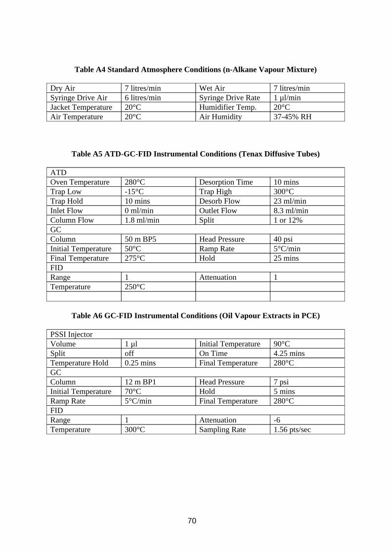
Table A4 Standard Atmosphere Conditions (n-Alkane Vapour Mixture)

Dry Air 7 litres/min Wet Air 7 litres/min Syringe Drive Air 6 litres/min Syringe Drive Rate 1 µl/min Jacket Temperature 20°C Humidifier Temp. 20°C Air Temperature 20°C Air Humidity 37-45% RH

Table A5 ATD-GC-FID Instrumental Conditions (Tenax Diffusive Tubes)

ATD Oven Temperature 280°C Desorption Time 10 mins Trap Low -15°C Trap High 300°C Trap Hold 10 mins Desorb Flow 23 ml/min Inlet Flow 0 ml/min Outlet Flow 8.3 ml/min Column Flow 1.8 ml/min Split 1 or 12% GC Column 50 m BP5 Head Pressure 40 psi Initial Temperature 50°C Ramp Rate 5°C/min Final Temperature 275°C Hold 25 mins FID Range 1 Attenuation 1 Temperature 250°C

Table A6 GC-FID Instrumental Conditions (Oil Vapour Extracts in PCE)

PSSI Injector Volume 1 µl Initial Temperature 90°C Split off On Time 4.25 mins Temperature Hold 0.25 mins Final Temperature 280°C GC Column 12 m BP1 Head Pressure 7 psi Initial Temperature 70°C Hold 5 mins Ramp Rate 5°C/min Final Temperature 280°C FID Range 1 Attenuation -6 Temperature 300°C Sampling Rate 1.56 pts/sec

70

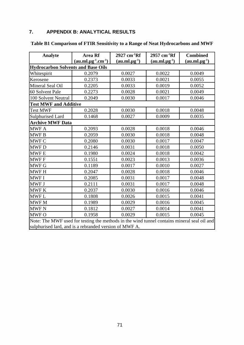
7. APPENDIX B: ANALYTICAL RESULTS

Table B1 Comparison of FTIR Sensitivity to a Range of Neat Hydrocarbons and MWF

Analyte Area Rf (au.ml.µg-1.cm-1)

2927 cm-1Rf (au.ml.µg-1)

2957 cm-1Rf (au.ml.µg-1)

Combined (au.ml.µg-1)

Hydrocarbon Solvents and Base Oils Whitespirit 0.2079 0.0027 0.0022 0.0049 Kerosene 0.2373 0.0033 0.0021 0.0055 Mineral Seal Oil 0.2205 0.0033 0.0019 0.0052 60 Solvent Pale 0.2273 0.0028 0.0021 0.0049 100 Solvent Neutral 0.2049 0.0030 0.0017 0.0046 Test MWF and Additive Test MWF 0.2028 0.0030 0.0018 0.0048 Sulphurised Lard 0.1468 0.0027 0.0009 0.0035 Archive MWF Data MWF A 0.2093 0.0028 0.0018 0.0046 MWF B 0.2059 0.0030 0.0018 0.0048 MWF C 0.2080 0.0030 0.0017 0.0047 MWF D 0.2146 0.0031 0.0018 0.0050 MWF E 0.1980 0.0024 0.0018 0.0042 MWF F 0.1551 0.0023 0.0013 0.0036 MWF G 0.1189 0.0017 0.0010 0.0027 MWF H 0.2047 0.0028 0.0018 0.0046 MWF I 0.2085 0.0031 0.0017 0.0048 MWF J 0.2111 0.0031 0.0017 0.0048 MWF K 0.2037 0.0030 0.0016 0.0046 MWF L 0.1808 0.0026 0.0015 0.0041 MWF M 0.1989 0.0029 0.0016 0.0045 MWF N 0.1812 0.0027 0.0014 0.0041 MWF O 0.1958 0.0029 0.0015 0.0045 Note: The MWF used for testing the methods in the wind tunnel contains mineral seal oil and sulphurised lard, and is a rebranded version of MWF A.

71

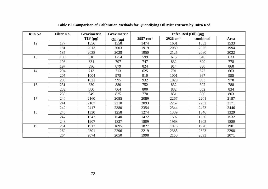
Table B2 Comparison of Calibration Methods for Quantifying Oil Mist Extracts by Infra Red

Run No. Filter No. Gravimetric Gravimetric Infra Red (Oil) (µg) TIP (µg) Oil (µg) 2957 cm-1 2926 cm-1 combined Area

12 177 1556 1558 1474 1601 1553 1533 181 2013 2003 1919 2089 2025 1994 185 2038 2028 1950 2125 2060 2022

13 189 610 <754 599 675 646 633 193 834 797 747 832 800 778 197 896 879 824 914 880 868

14 204 713 713 625 701 672 663 205 1004 975 910 1001 967 955 206 1021 995 932 1029 993 978

16 231 830 880 752 832 802 788 232 880 864 800 882 852 834 233 849 825 770 851 820 803

17 240 2160 2085 2089 2267 2201 2187 241 2187 2210 2093 2267 2202 2171 242 2417 2380 2354 2544 2473 2446

18 246 1330 1258 1274 1389 1346 1329 247 1547 1540 1472 1597 1550 1532 248 1907 1837 1809 1963 1905 1880

19 261 1913 1895 1827 1975 1920 1901 262 2301 2296 2219 2385 2323 2298 264 2074 2050 1998 2150 2093 2071

72

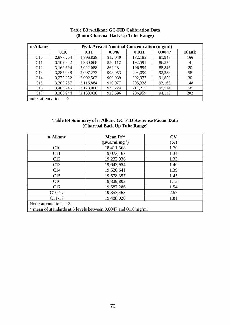
Table B3 n-Alkane GC-FID Calibration Data (8 mm Charcoal Back Up Tube Range)

n-Alkane Peak Area at Nominal Concentration (mg/ml) 0.16 0.11 0.046 0.011 0.0047 Blank

C10 2,977,204 1,896,828 812,040 182,185 81,945 166 C11 3,102,342 1,980,068 850,112 192,591 86,576 4 C12 3,169,694 2,022,088 869,231 196,599 88,846 20 C13 3,285,948 2,097,273 903,053 204,090 92,283 58 C14 3,275,352 2,092,563 900,039 202,977 91,850 30 C15 3,309,287 2,116,884 910,077 205,338 93,163 148 C16 3,403,746 2,178,000 935,224 211,215 95,514 58 C17 3,366,944 2,153,028 923,696 206,959 94,132 202

note: attenuation = -3

Table B4 Summary of n-Alkane GC-FID Response Factor Data (Charcoal Back Up Tube Range)

n-Alkane Mean Rf* (µv.s.ml.mg-1)

CV (%)

C10 18,411,568 1.70 C11 19,022,162 1.34 C12 19,233,936 1.32 C13 19,643,954 1.40 C14 19,520,641 1.39 C15 19,578,357 1.45 C16 19,829,803 1.15 C17 19,587,286 1.54

C10-17 19,353,463 2.57 C11-17 19,488,020 1.81

Note: attenuation = -3 * mean of standards at 5 levels between 0.0047 and 0.16 mg/ml

73

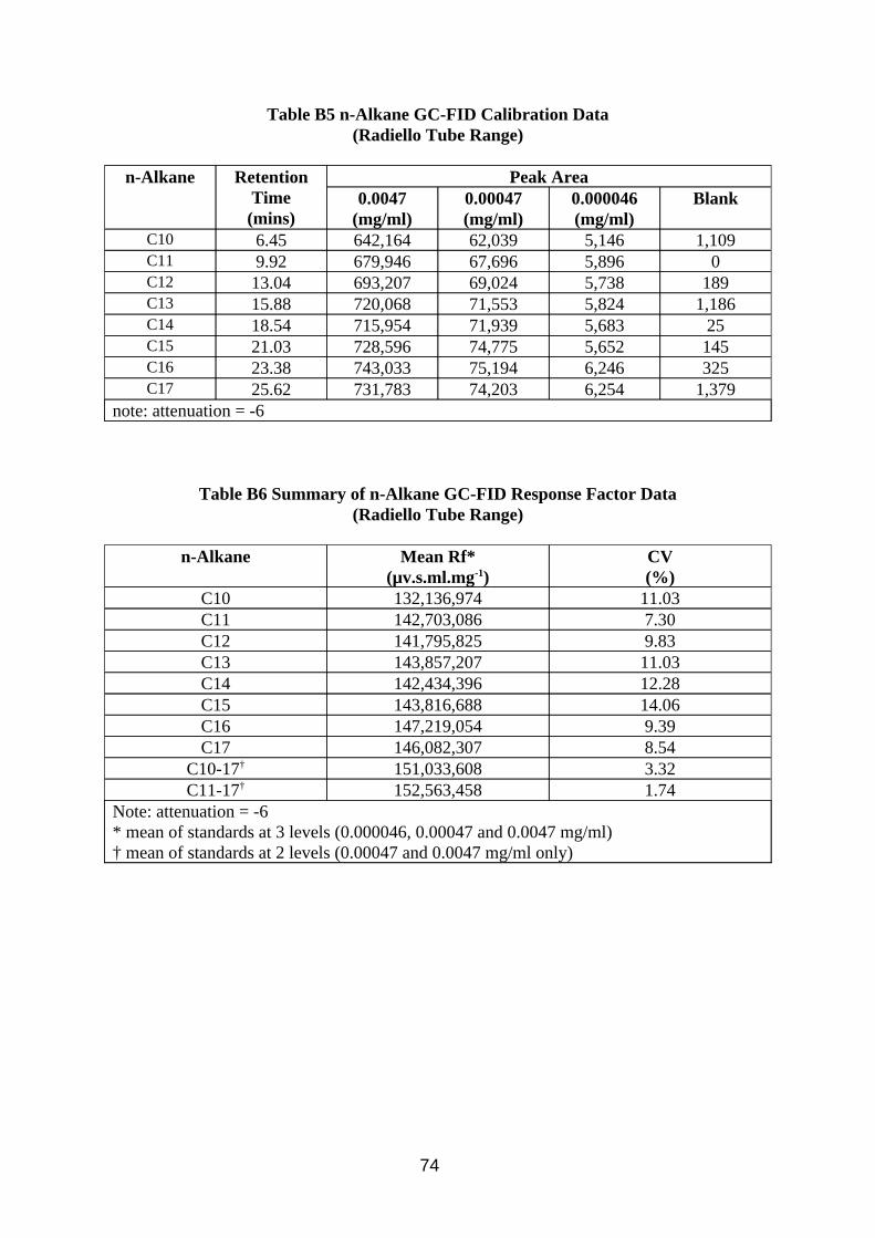
Table B5 n-Alkane GC-FID Calibration Data (Radiello Tube Range)

n-Alkane Retention Time (mins)

Peak Area 0.0047

(mg/ml) 0.00047 (mg/ml)

0.000046 (mg/ml)

Blank

C10 6.45 642,164 62,039 5,146 1,109 C11 9.92 679,946 67,696 5,896 0 C12 13.04 693,207 69,024 5,738 189 C13 15.88 720,068 71,553 5,824 1,186 C14 18.54 715,954 71,939 5,683 25 C15 21.03 728,596 74,775 5,652 145 C16 23.38 743,033 75,194 6,246 325 C17 25.62 731,783 74,203 6,254 1,379

note: attenuation = -6

Table B6 Summary of n-Alkane GC-FID Response Factor Data (Radiello Tube Range)

n-Alkane Mean Rf* (µv.s.ml.mg-1)

CV (%)

C10 132,136,974 11.03 C11 142,703,086 7.30 C12 141,795,825 9.83 C13 143,857,207 11.03 C14 142,434,396 12.28 C15 143,816,688 14.06 C16 147,219,054 9.39 C17 146,082,307 8.54

C10-17† 151,033,608 3.32 C11-17† 152,563,458 1.74

Note: attenuation = -6 * mean of standards at 3 levels (0.000046, 0.00047 and 0.0047 mg/ml) † mean of standards at 2 levels (0.00047 and 0.0047 mg/ml only)

74

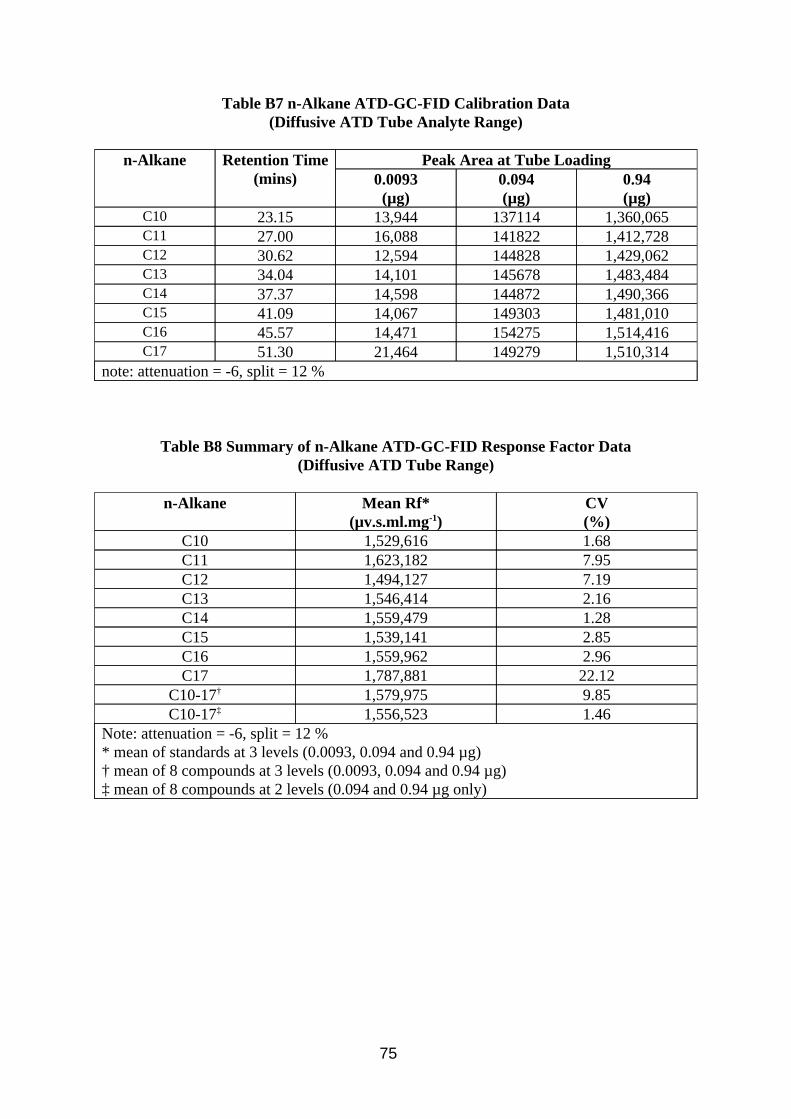
Table B7 n-Alkane ATD-GC-FID Calibration Data (Diffusive ATD Tube Analyte Range)

n-Alkane Retention Time (mins)

Peak Area at Tube Loading 0.0093 (µg)

0.094 (µg)

0.94 (µg)

C10 23.15 13,944 137114 1,360,065 C11 27.00 16,088 141822 1,412,728 C12 30.62 12,594 144828 1,429,062 C13 34.04 14,101 145678 1,483,484 C14 37.37 14,598 144872 1,490,366 C15 41.09 14,067 149303 1,481,010 C16 45.57 14,471 154275 1,514,416 C17 51.30 21,464 149279 1,510,314

note: attenuation = -6, split = 12 %

Table B8 Summary of n-Alkane ATD-GC-FID Response Factor Data (Diffusive ATD Tube Range)

n-Alkane Mean Rf* (µv.s.ml.mg-1)

CV (%)

C10 1,529,616 1.68 C11 1,623,182 7.95 C12 1,494,127 7.19 C13 1,546,414 2.16 C14 1,559,479 1.28 C15 1,539,141 2.85 C16 1,559,962 2.96 C17 1,787,881 22.12

C10-17† 1,579,975 9.85 C10-17‡ 1,556,523 1.46

Note: attenuation = -6, split = 12 % * mean of standards at 3 levels (0.0093, 0.094 and 0.94 µg) † mean of 8 compounds at 3 levels (0.0093, 0.094 and 0.94 µg) ‡ mean of 8 compounds at 2 levels (0.094 and 0.94 µg only)

75

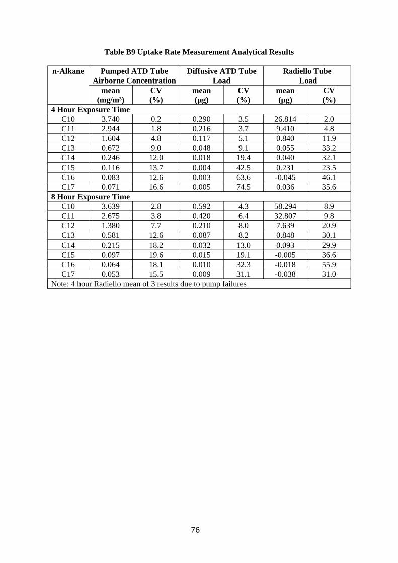
Table B9 Uptake Rate Measurement Analytical Results

n-Alkane Pumped ATD Tube Airborne Concentration

Diffusive ATD Tube Load

Radiello Tube Load

mean (mg/m³)

CV (%)

mean (µg)

CV (%)

mean (µg)

CV (%)

4 Hour Exposure Time C10 3.740 0.2 0.290 3.5 26.814 2.0 C11 2.944 1.8 0.216 3.7 9.410 4.8 C12 1.604 4.8 0.117 5.1 0.840 11.9 C13 0.672 9.0 0.048 9.1 0.055 33.2 C14 0.246 12.0 0.018 19.4 0.040 32.1 C15 0.116 13.7 0.004 42.5 0.231 23.5 C16 0.083 12.6 0.003 63.6 -0.045 46.1 C17 0.071 16.6 0.005 74.5 0.036 35.6

8 Hour Exposure Time C10 3.639 2.8 0.592 4.3 58.294 8.9 C11 2.675 3.8 0.420 6.4 32.807 9.8 C12 1.380 7.7 0.210 8.0 7.639 20.9 C13 0.581 12.6 0.087 8.2 0.848 30.1 C14 0.215 18.2 0.032 13.0 0.093 29.9 C15 0.097 19.6 0.015 19.1 -0.005 36.6 C16 0.064 18.1 0.010 32.3 -0.018 55.9 C17 0.053 15.5 0.009 31.1 -0.038 31.0

Note: 4 hour Radiello mean of 3 results due to pump failures

76

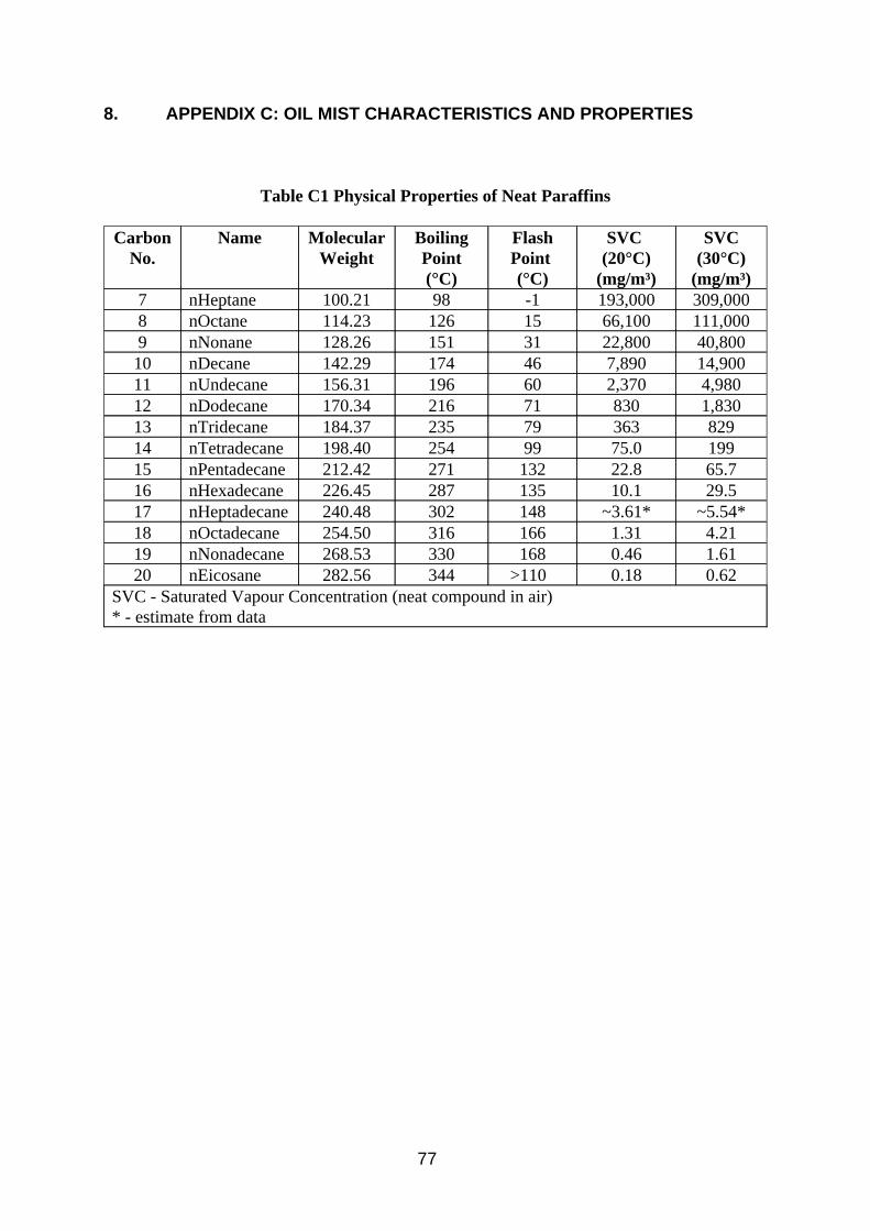
8. APPENDIX C: OIL MIST CHARACTERISTICS AND PROPERTIES

Table C1 Physical Properties of Neat Paraffins

Carbon No.

Name Molecular Weight

Boiling Point (°C)

Flash Point (°C)

SVC (20°C)

(mg/m³)

SVC (30°C)

(mg/m³) 7 nHeptane 100.21 98 -1 193,000 309,000 8 nOctane 114.23 126 15 66,100 111,000 9 nNonane 128.26 151 31 22,800 40,800

10 nDecane 142.29 174 46 7,890 14,900 11 nUndecane 156.31 196 60 2,370 4,980 12 nDodecane 170.34 216 71 830 1,830 13 nTridecane 184.37 235 79 363 829 14 nTetradecane 198.40 254 99 75.0 199 15 nPentadecane 212.42 271 132 22.8 65.7 16 nHexadecane 226.45 287 135 10.1 29.5 17 nHeptadecane 240.48 302 148 ~3.61* ~5.54* 18 nOctadecane 254.50 316 166 1.31 4.21 19 nNonadecane 268.53 330 168 0.46 1.61 20 nEicosane 282.56 344 >110 0.18 0.62

SVC - Saturated Vapour Concentration (neat compound in air) * - estimate from data

77

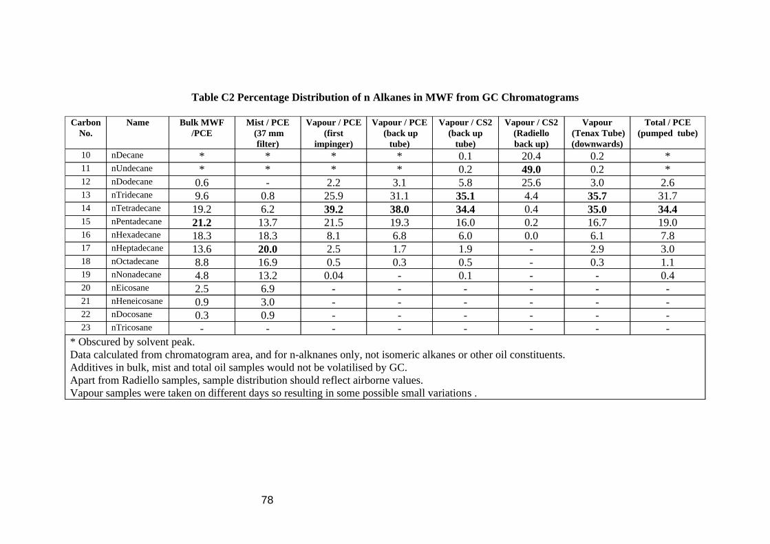
Table C2 Percentage Distribution of n Alkanes in MWF from GC Chromatograms

Carbon No.

Name Bulk MWF /PCE

Mist / PCE (37 mm

filter)

Vapour / PCE (first

impinger)

Vapour / PCE (back up

tube)

Vapour / CS2 (back up

tube)

Vapour / CS2 (Radiello back up)

Vapour (Tenax Tube) (downwards)

Total / PCE (pumped tube)

10 nDecane * * * * 0.1 20.4 0.2 * 11 nUndecane * * * * 0.2 49.0 0.2 * 12 nDodecane 0.6 - 2.2 3.1 5.8 25.6 3.0 2.6 13 nTridecane 9.6 0.8 25.9 31.1 35.1 4.4 35.7 31.7 14 nTetradecane 19.2 6.2 39.2 38.0 34.4 0.4 35.0 34.4 15 nPentadecane 21.2 13.7 21.5 19.3 16.0 0.2 16.7 19.0 16 nHexadecane 18.3 18.3 8.1 6.8 6.0 0.0 6.1 7.8 17 nHeptadecane 13.6 20.0 2.5 1.7 1.9 - 2.9 3.0 18 nOctadecane 8.8 16.9 0.5 0.3 0.5 - 0.3 1.1 19 nNonadecane 4.8 13.2 0.04 - 0.1 - - 0.4 20 nEicosane 2.5 6.9 - - - - - -21 nHeneicosane 0.9 3.0 - - - - - -22 nDocosane 0.3 0.9 - - - - - -23 nTricosane - - - - - - - -

* Obscured by solvent peak. Data calculated from chromatogram area, and for n-alknanes only, not isomeric alkanes or other oil constituents. Additives in bulk, mist and total oil samples would not be volatilised by GC. Apart from Radiello samples, sample distribution should reflect airborne values. Vapour samples were taken on different days so resulting in some possible small variations .

78

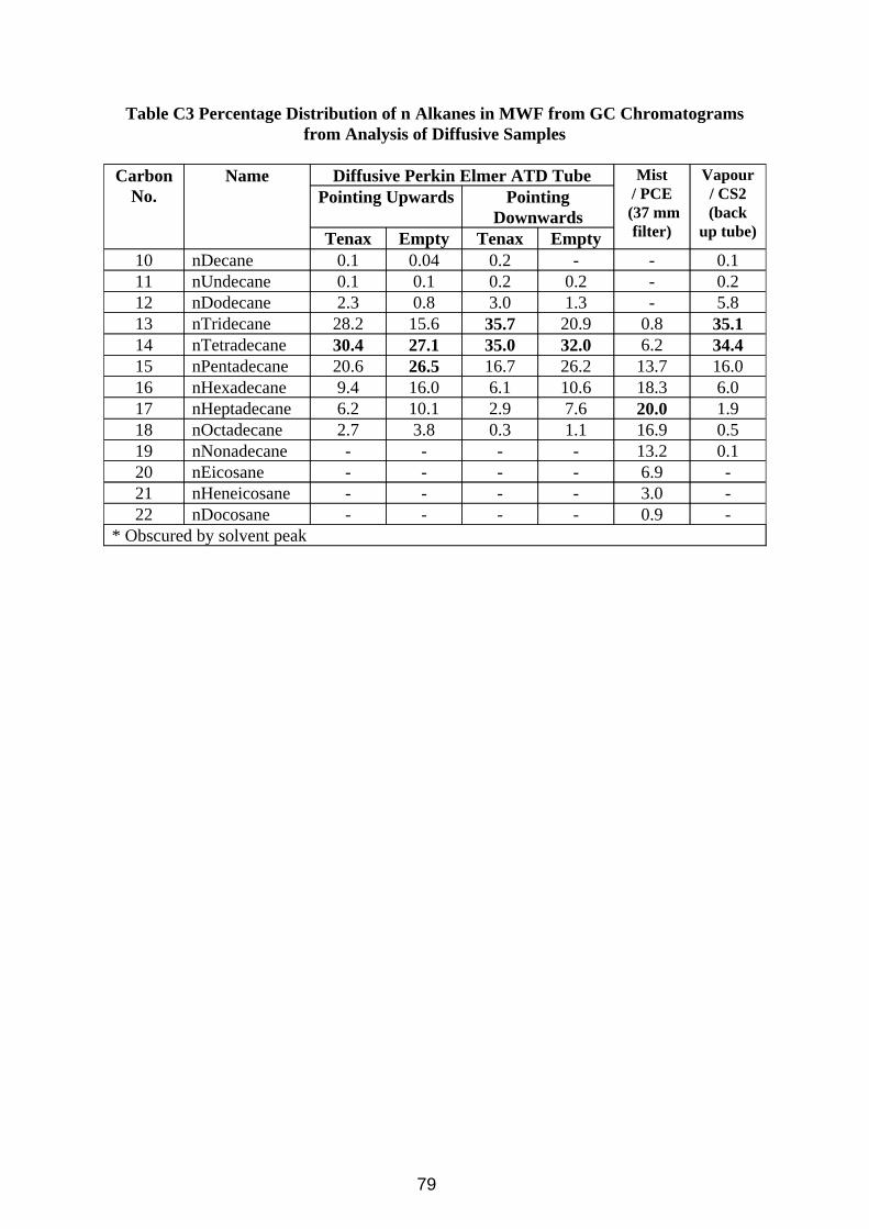
Table C3 Percentage Distribution of n Alkanes in MWF from GC Chromatograms from Analysis of Diffusive Samples

Carbon No.

Name Diffusive Perkin Elmer ATD Tube Mist / PCE

(37 mm filter)

Vapour / CS2 (back

up tube)

Pointing Upwards Pointing Downwards

Tenax Empty Tenax Empty 10 nDecane 0.1 0.04 0.2 - - 0.1 11 nUndecane 0.1 0.1 0.2 0.2 - 0.2 12 nDodecane 2.3 0.8 3.0 1.3 - 5.8 13 nTridecane 28.2 15.6 35.7 20.9 0.8 35.1 14 nTetradecane 30.4 27.1 35.0 32.0 6.2 34.4 15 nPentadecane 20.6 26.5 16.7 26.2 13.7 16.0 16 nHexadecane 9.4 16.0 6.1 10.6 18.3 6.0 17 nHeptadecane 6.2 10.1 2.9 7.6 20.0 1.9 18 nOctadecane 2.7 3.8 0.3 1.1 16.9 0.5 19 nNonadecane - - - - 13.2 0.1 20 nEicosane - - - - 6.9 -21 nHeneicosane - - - - 3.0 -22 nDocosane - - - - 0.9 -

* Obscured by solvent peak

79

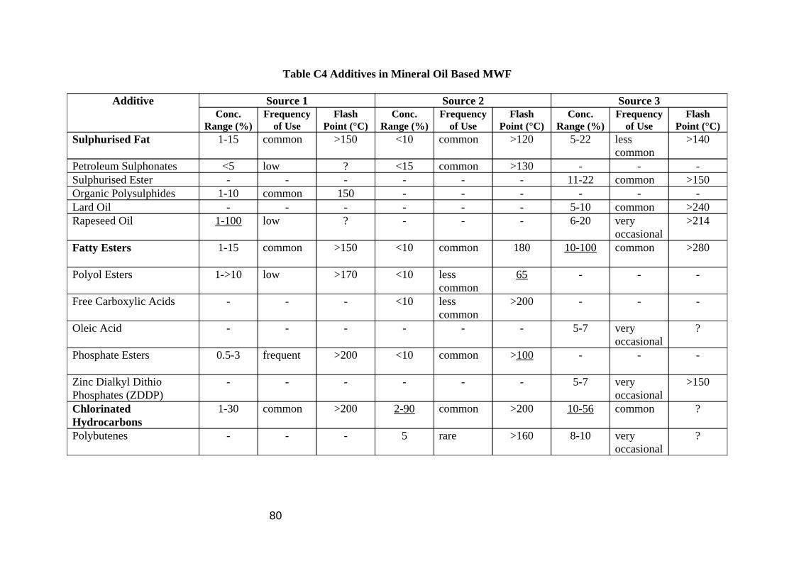
Table C4 Additives in Mineral Oil Based MWF

Additive Source 1 Source 2 Source 3 Conc. Frequency Flash Conc. Frequency Flash Conc. Frequency Flash

Range (%) of Use Point (°C) Range (%) of Use Point (°C) Range (%) of Use Point (°C) Sulphurised Fat 1-15 common >150 <10 common >120 5-22 less >140

common Petroleum Sulphonates <5 low ? <15 common >130 - - -Sulphurised Ester - - - - - - 11-22 common >150 Organic Polysulphides 1-10 common 150 - - - - - -Lard Oil - - - - - - 5-10 common >240 Rapeseed Oil 1-100 low ? - - - 6-20 very

occasional >214

Fatty Esters 1-15 common >150 <10 common 180 10-100 common >280

Polyol Esters 1->10 low >170 <10 less common

65 - - -

Free Carboxylic Acids - - - <10 less common

>200 - - -

Oleic Acid - - - - - - 5-7 very occasional

?

Phosphate Esters 0.5-3 frequent >200 <10 common >100 - - -

Zinc Dialkyl Dithio Phosphates (ZDDP)

- - - - - - 5-7 very occasional

>150

Chlorinated 1-30 common >200 2-90 common >200 10-56 common ? Hydrocarbons Polybutenes - - - 5 rare >160 8-10 very

occasional ?

80

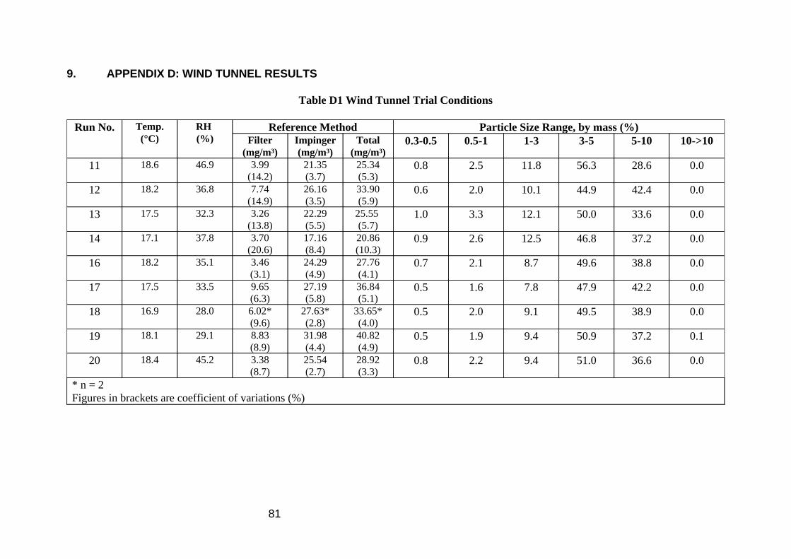
9. APPENDIX D: WIND TUNNEL RESULTS

Table D1 Wind Tunnel Trial Conditions

Run No. Temp. (°C)

RH (%)

Reference Method Particle Size Range, by mass (%) Filter Impinger Total 0.3-0.5 0.5-1 1-3 3-5 5-10 10->10

(mg/m³) (mg/m³) (mg/m³) 11 18.6 46.9 3.99 21.35 25.34 0.8 2.5 11.8 56.3 28.6 0.0

(14.2) (3.7) (5.3) 12 18.2 36.8 7.74 26.16 33.90 0.6 2.0 10.1 44.9 42.4 0.0

(14.9) (3.5) (5.9) 13 17.5 32.3 3.26 22.29 25.55 1.0 3.3 12.1 50.0 33.6 0.0

(13.8) (5.5) (5.7) 14 17.1 37.8 3.70 17.16 20.86 0.9 2.6 12.5 46.8 37.2 0.0

(20.6) (8.4) (10.3) 16 18.2 35.1 3.46 24.29 27.76 0.7 2.1 8.7 49.6 38.8 0.0

(3.1) (4.9) (4.1) 17 17.5 33.5 9.65 27.19 36.84 0.5 1.6 7.8 47.9 42.2 0.0

(6.3) (5.8) (5.1) 18 16.9 28.0 6.02* 27.63* 33.65* 0.5 2.0 9.1 49.5 38.9 0.0

(9.6) (2.8) (4.0) 19 18.1 29.1 8.83 31.98 40.82 0.5 1.9 9.4 50.9 37.2 0.1

(8.9) (4.4) (4.9) 20 18.4 45.2 3.38 25.54 28.92 0.8 2.2 9.4 51.0 36.6 0.0

(8.7) (2.7) (3.3) * n = 2 Figures in brackets are coefficient of variations (%)

81

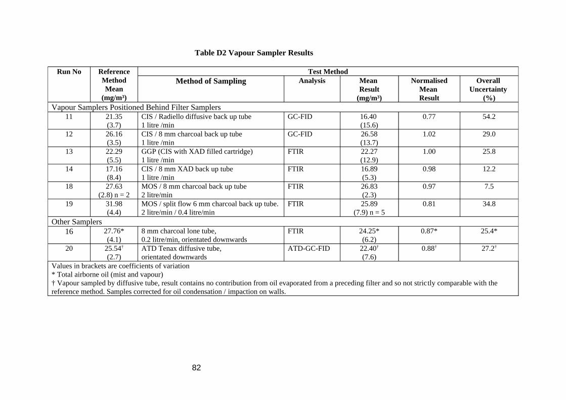
Table D2 Vapour Sampler Results

Run No Reference Method Mean

(mg/m³)

Test Method Method of Sampling Analysis Mean

Result (mg/m³)

Normalised Mean Result

Overall Uncertainty

(%) Vapour Samplers Positioned Behind Filter Samplers

11 21.35 (3.7)

CIS / Radiello diffusive back up tube 1 litre /min

GC-FID 16.40 (15.6)

0.77 54.2

12 26.16 (3.5)

CIS / 8 mm charcoal back up tube 1 litre /min

GC-FID 26.58 (13.7)

1.02 29.0

13 22.29 (5.5)

GGP (CIS with XAD filled cartridge) 1 litre /min

FTIR 22.27 (12.9)

1.00 25.8

14 17.16 (8.4)

CIS / 8 mm XAD back up tube 1 litre /min

FTIR 16.89 (5.3)

0.98 12.2

18 27.63 (2.8) n = 2

MOS / 8 mm charcoal back up tube 2 litre/min

FTIR 26.83 (2.3)

0.97 7.5

19 31.98 (4.4)

MOS / split flow 6 mm charcoal back up tube. 2 litre/min / 0.4 litre/min

FTIR 25.89 (7.9) n = 5

0.81 34.8

Other Samplers 16 27.76*

(4.1) 8 mm charcoal lone tube, 0.2 litre/min, orientated downwards

FTIR 24.25* (6.2)

0.87* 25.4*

20 25.54†

(2.7) ATD Tenax diffusive tube, orientated downwards

ATD-GC-FID 22.40†

(7.6) 0.88† 27.2†

Values in brackets are coefficients of variation * Total airborne oil (mist and vapour) † Vapour sampled by diffusive tube, result contains no contribution from oil evaporated from a preceding filter and so not strictly comparable with the reference method. Samples corrected for oil condensation / impaction on walls.

82

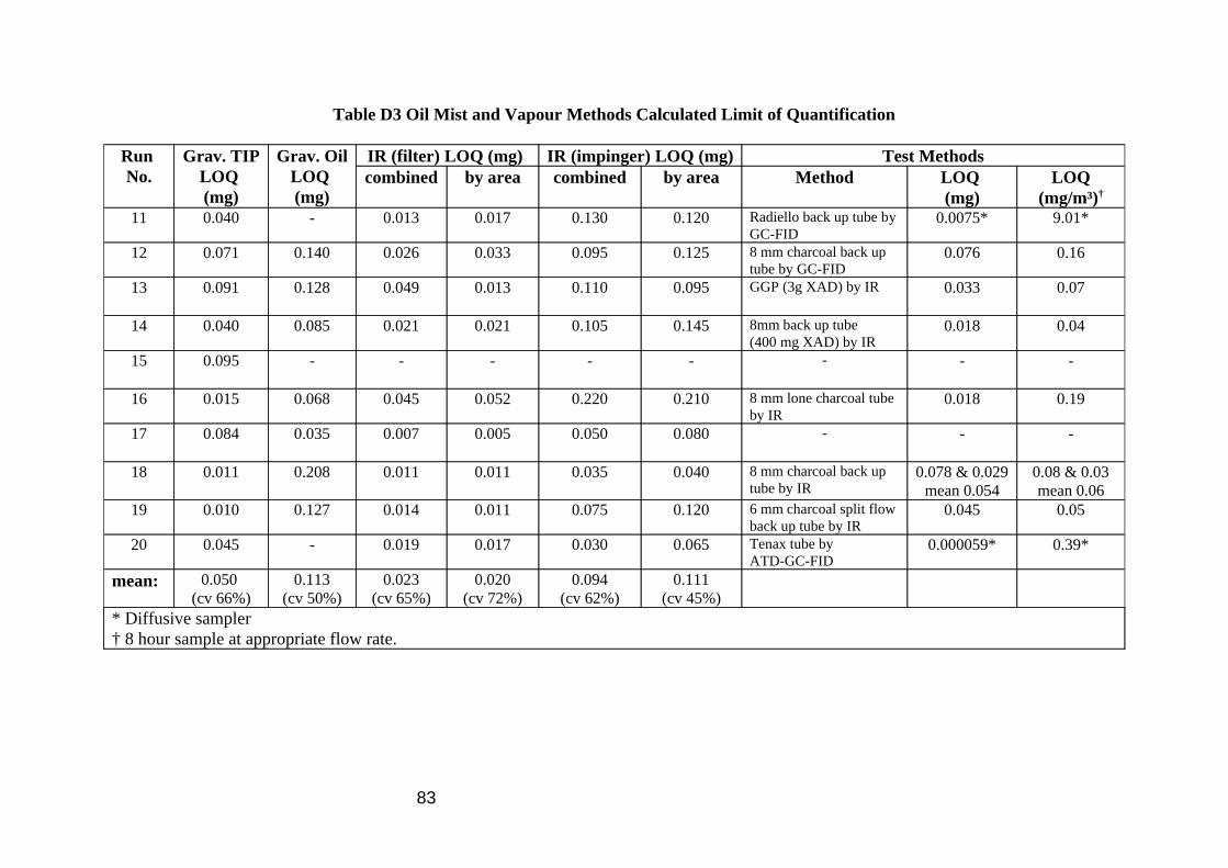
Table D3 Oil Mist and Vapour Methods Calculated Limit of Quantification

Run No.

Grav. TIP LOQ (mg)

Grav. Oil LOQ (mg)

IR (filter) LOQ (mg) IR (impinger) LOQ (mg) Test Methods combined by area combined by area Method LOQ

(mg) LOQ

(mg/m³)†

11 0.040 - 0.013 0.017 0.130 0.120 Radiello back up tube by GC-FID

0.0075* 9.01*

12 0.071 0.140 0.026 0.033 0.095 0.125 8 mm charcoal back up tube by GC-FID

0.076 0.16

13 0.091 0.128 0.049 0.013 0.110 0.095 GGP (3g XAD) by IR 0.033 0.07

14 0.040 0.085 0.021 0.021 0.105 0.145 8mm back up tube (400 mg XAD) by IR

0.018 0.04

15 0.095 - - - - - - - -

16 0.015 0.068 0.045 0.052 0.220 0.210 8 mm lone charcoal tube by IR

0.018 0.19

17 0.084 0.035 0.007 0.005 0.050 0.080 - - -

18 0.011 0.208 0.011 0.011 0.035 0.040 8 mm charcoal back up tube by IR

0.078 & 0.029 mean 0.054

0.08 & 0.03 mean 0.06

19 0.010 0.127 0.014 0.011 0.075 0.120 6 mm charcoal split flow back up tube by IR

0.045 0.05

20 0.045 - 0.019 0.017 0.030 0.065 Tenax tube by ATD-GC-FID

0.000059* 0.39*

mean: 0.050 (cv 66%)

0.113 (cv 50%)

0.023 (cv 65%)

0.020 (cv 72%)

0.094 (cv 62%)

0.111 (cv 45%)

* Diffusive sampler † 8 hour sample at appropriate flow rate.

83

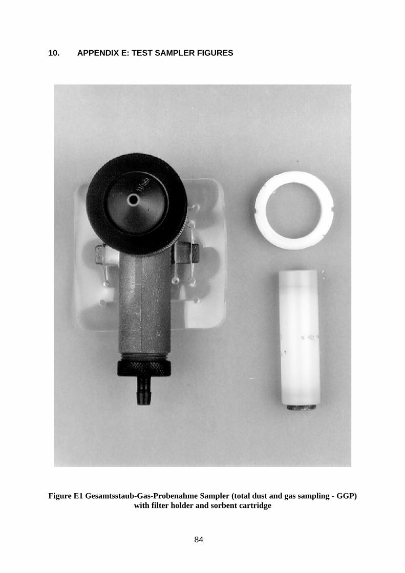
10. APPENDIX E: TEST SAMPLER FIGURES

Figure E1 Gesamtsstaub-Gas-Probenahme Sampler (total dust and gas sampling - GGP) with filter holder and sorbent cartridge

84

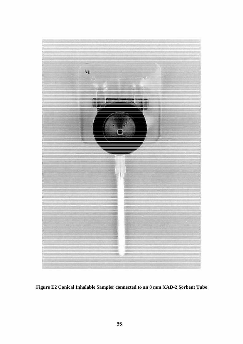
Figure E2 Conical Inhalable Sampler connected to an 8 mm XAD-2 Sorbent Tube

85

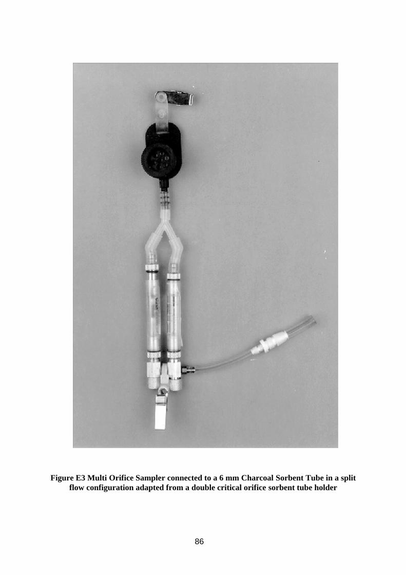
Figure E3 Multi Orifice Sampler connected to a 6 mm Charcoal Sorbent Tube in a split flow configuration adapted from a double critical orifice sorbent tube holder

86

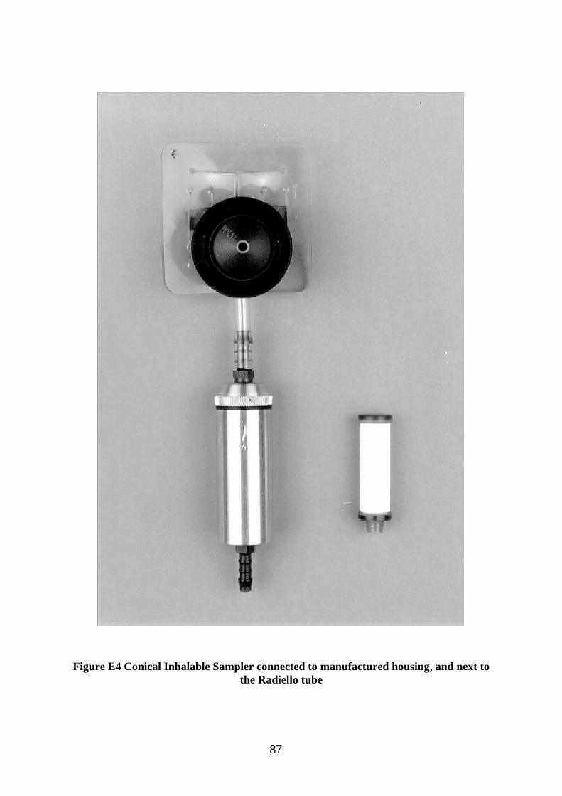
Figure E4 Conical Inhalable Sampler connected to manufactured housing, and next to the Radiello tube

87