arX

iv:1

206.

3704

v1 [

mat

h.C

T]

16

Jun

2012

Lax Diagrams and Enrichment

Hugo V. Bacard ∗

Laboratoire J.-A. Dieudonné, UNS

Abstract

We introduce a new type of weakly enriched categories over a given symmetric monoidalmodel category M ; these are called Co-Segal categories. Their definition derives from thephilosophy of classical (enriched) Segal categories. We study their homotopy theory by givinga model structure on them. One of the motivations of introducing these structure was to havean alternative definition of higher linear categories following Segal-like methods.

Contents

1 Introduction 2

2 Lax Diagrams 5

3 Operads and Lax morphisms 6

4 Co-Segal Categories 17

5 Properties of MS(C) 28

6 Locally Reedy 2-categories 32

7 A model structure on MS(X) 45

8 Variation of the set of objects 53

9 Co-Segalification of S-diagrams 60

10 A model structure for M -Cat for a 2-category M 90

A Some classical lemma 94

B Adjunction Lemma 98

C MS(X) is cocomplete if M is so 107

D LaxO-alg(C.,M.) is locally presentable 112

∗This research is supported in part by the Agence Nationale de la Recherche grant ANR-09-BLAN-0151-02(HODAG)

1

E Pushout in LaxO-alg(C.,M.) 122

1 Introduction

In this paper we pursue the idea initiated in [3], of having a theory of weakly enriched categoriesover a symmetric monoidal model category M = (M,⊗, I). We introduce the notion of Co-SegalM -category. Before going to what motivated the consideration of these ‘categories’ we present verybriefly hereafter the main philosophy.

In a classical M -category C, for every triple (A,B,C) of objects of C, the composition is givenby a map of M :

C(A,B)⊗ C(B,C) −→ C(A,C).

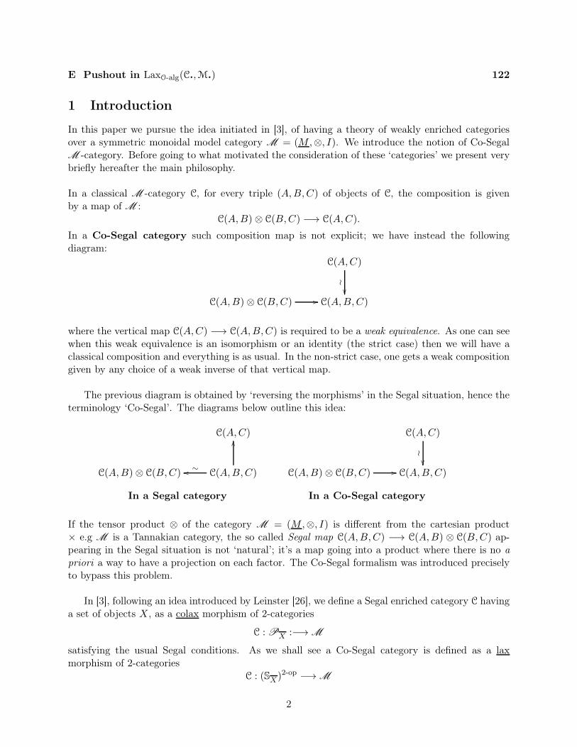
In a Co-Segal category such composition map is not explicit; we have instead the followingdiagram:

C(A,B)⊗ C(B,C) C(A,B,C)

C(A,C)

//

≀

��

where the vertical map C(A,C) −→ C(A,B,C) is required to be a weak equivalence. As one can seewhen this weak equivalence is an isomorphism or an identity (the strict case) then we will have aclassical composition and everything is as usual. In the non-strict case, one gets a weak compositiongiven by any choice of a weak inverse of that vertical map.

The previous diagram is obtained by ‘reversing the morphisms’ in the Segal situation, hence theterminology ‘Co-Segal’. The diagrams below outline this idea:

C(A,B)⊗ C(B,C) C(A,B,C)

C(A,C)

∼oo

OO

In a Segal category

C(A,B)⊗ C(B,C) C(A,B,C)

C(A,C)

//

≀

��

In a Co-Segal category

If the tensor product ⊗ of the category M = (M,⊗, I) is different from the cartesian product× e.g M is a Tannakian category, the so called Segal map C(A,B,C) −→ C(A,B) ⊗ C(B,C) ap-pearing in the Segal situation is not ‘natural’; it’s a map going into a product where there is no apriori a way to have a projection on each factor. The Co-Segal formalism was introduced preciselyto bypass this problem.

In [3], following an idea introduced by Leinster [26], we define a Segal enriched category C havinga set of objects X, as a colax morphism of 2-categories

C : PX :−→M

satisfying the usual Segal conditions. As we shall see a Co-Segal category is defined as a laxmorphism of 2-categories

C : (SX)2-op −→M

2

satisfying the Co-Segal conditions (Definition 4.7 ). Here PX is a 2-category over ∆ while SX ⊂PX

is over ∆epi. These 2-categories are probably example of what should be a locally Reedy 2-category,that is a 2-category such that each category of 1-morphisms is a Reedy category and the compositionis coherent with the Reedy structures.

To develop a homotopy theory of these Co-Segal categories we follow the same philosophyas for Segal categories, that is we consider the more general objects consisting of lax morphismsC : (SX)

2-op −→M without demanding the Co-Segal conditions yet; these are called Pre-Co-Segalcategories.

As X runs through Set we have a category MS(Set) of all Pre-Co-Segal categories with mor-phisms between them. We have a natural Grothendieck bifibration Ob : MS(Set) −→ Set.

The main result of this paper is the following

Theorem. Let M be a symmetric monoidal model category which is cofibrantly generated and suchthat all the objects are cofibrant. Then the following holds.

1. the category MS(Set), of Pre-Co-Segal categories admits a model structure which is cofibrantlygenerated,

2. fibrant objects are Co-Segal categories,

3. If M is combinatorial then so is MS(Set).

Plan of the paper

We begin the paper by the definition of a lax diagram in a 2-category M , which are simply laxfunctors of 2-category in the sense of Bénabou [5]. We point out that M -categories are special casesof lax diagrams as earlier observed by Street [38].

Then in section 3 we recall some basic definitions about multisorted operads or colored operads.The idea is to use the powerful language of operads to treat 2-categories and lax morphisms interms of O-algebras and lax morphisms of O-algebras for some suitable operad. The operads we’reworking with are the ones enriched in Cat.

Given two O-algebras C. and M. there is a category LaxO-alg(C.,M.) of lax morphisms andmorphism of lax morphisms. After setting up some definitions we prove that:

• for a locally presentable O-algebra M. the category LaxO-alg(C.,M.) is also locally presentable(Theorem 3.8);

• If M. is a special Quillen O-algebra (Definition 3.9) and under some hypothesis, the categoryLaxO-alg(C.,M.) carries a model structure (Theorem 3.12).

In section 4 we introduce the language of Co-Segal categories starting with an overview of theone-object case. We’ve tried as much as possible to make this section independent from the previousones. We only use the language of lax functor between 2-categories rather than lax morphisms ofO-algebras. We introduce first the notion of an S-diagram in M which correspond to Pre-Co-Segalcategories (Definition 4.6). Then we define a Co-Segal category to be an S-diagram satisfying theCo-Segal conditions (Definition 4.8). After giving some definitions we show that

• A strict Co-Segal M -category is the same thing as a strict (semi) M -category (Proposition4.11);

3

• The Co-Segal conditions are stable under weak equivalences (Proposition 4.14).

In section 5 we show that the category MS(X) of Pre-Co-Segal categories with a fixed set ofobjects X is:

• is cocomplete if M is so (Theorem 5.2) ; and

• locally presentable if M is so (Theorem 5.1).

For both of these two theorems, we’ve presented a ‘direct proof’ i.e which doesn’t make use of thelanguage of operads; the idea is to make the content accessible for a reader who is not familiar withoperads.

In section 6 we consider the notion of locally Reedy 2-category. The main idea is to provide adirect model structure on the category MS(X) (Corollary 6.15).

In section 7 we give two type of model structures on MS(X), using a different method. Thesemodel structures play an important role in the later sections. We show precisely that if M is asymmetric monoidal model category, which is cofibrantly generated and such that all the objectsare cofibrant, then we have:

• a projective model structure on MS(X) denoted MS(X)proj (Theorem 7.6);

• an injective model structure on MS(X) denoted MS(X)inj (Theorem 7.7);

• the identity functor Id : MS(X)proj ⇄MS(X)inj : Id is a Quillen equivalence (Corollary 7.8);

These model structures are both cofibrantly generated (and combinatorial if M is so). The projec-tive model structure is the same as the one given by Corollary 6.15.

The section 8 is dedicated to study of the category MS(Set) of all Pre-Co-Segal categories. Weshow that:

• MS(Set) inherits the cocompleteness and local presentability of M (Theorem 8.2); and

• that MS(Set) carries a fibered projective model strucuture which is cofibrantly generated. Andif M is combinatorial then so is MS(Set) (Theorem 8.8 and Corollary 8.11).

In section 9, we begin by constructing for each set X, an endofunctor S : MS(X) −→MS(X),called ‘Co-Segalifcation’ which takes any Pre-Co-Segal category to a Co-Segal category (Proposition9.7). Assuming that MS(X) is left proper if M is so (Hypothesis 9.2.3.1) we prove that:

• There exists a new injective model structure on MS(X) denoted MS(X)+inj which is combina-

torial and such that the fibrant objects are Co-Segal categories. MS(X)+inj is the left Bousfield

localization of MS(X)inj with respect to some set of maps Kinj (Theorem 9.12).

• There is also a new projective model structure on MS(X) denoted MS(X)+proj which is com-

binatorial and such that the fibrant objects are Co-Segal categories. The model categoryMS(X)

+proj is the left Bousfield localization of MS(X)proj with respect to some set of maps

Kproj (Theorem 9.21).

4

• We have also a new fibered projective model structure on MS(Set) denoted MS(Set)+proj whichis combinatorial and such that the fibrant objects are Co-Segal categories (Theorem 9.24).

In section 10 we reviewed the basics about M -categories for a 2-category M . For a fixed setof objects X, we show that if M is locally a model category (Definition 10.1) and all the objectsare cofibrant, then the category M -Cat(X) has a model structure which is cofibrantly generatedand combinatorial if M is so. We leave the reader who might be interested to give a fibered modelstructure on M -Cat and even the ‘canonical model structure’ in the sense of Berger-Moedijk [7].

It seems clear that all the previous results on Co-Segal categories should hold if we replace themonoidal model category M by a 2-category which is locally a model category.

Acknowledgments. I would like to warmly thank my supervisor Carlos Simpson for his supportand encouragement. This work owes him a lot. This paper is an extension of a previous workoriginally motivated by a question of Julie Bergner and Tom Leinster; their ideas have undoubtedlyinfluenced this work. I would like to thank Jacob Lurie for helpful conversations. I would also liketo thank Bertrand Toën for helpful comments.

2 Lax Diagrams

In the following we fix M a bicategory (or 2-category). For a sufficiently large universe V we willassume that all the 2-categories we will consider (including M ) have a V-small set of 2-morphisms.

Definition 2.1. A lax diagram in M is a lax morphism F : D −→ M , where D is a strict2-category.

For each D we will consider Lax(D,M ) the 1-category of lax morphisms from D to M andicons in the sense of Lack [24].

− The objects of Lax(D,M ) are lax morphisms,− the morphisms are icons (see [24]) .

Icons are what we call later simple transformations (Definition 4.12). The reader can find forexample in [24, 25] these definitions.

Warning. Note that in general there is only a bicategory and (not a 2-category) of lax morphisms.This bicategory is described as follows

− The objects of are lax morphisms,− the 1-morphisms are transformations of lax morphisms,− the 2-morphisms are modifications of transformations.

By definition of a lax morphism F : D −→ M we have a function between the correspondingset of objects

Ob(F ) : Ob(D) −→ Ob(M ).

This defines a function Ob : Ob[Lax(D,M )] −→ Hom[Ob(D),Ob(M )] which sends F to Ob(F ).

Given a function φ from Ob(D) to Ob(M ) we will say that F ∈ Lax(D,M ) is over φ ifOb(F ) = φ. We will denote by Lax/φ(D,M ) be the full subcategory of Lax(D,M ) consisting ofobjects over φ and transformations of lax morphisms.

5

M -categories are lax morphisms Given an M -category C having a set of objects X, then wecan define a lax morphism denoted again C : X −→M . Here X is the universal nontrivial groupoidassociated to X; we refer it as the undiscrete or coarse category associated to X. In this contextone interprets the lax morphism as the nerve of the enriched category.

This identification of M -categories as lax morphisms goes back to Bénabou [5] as pointed outby Street [38]. Bénabou defined them as polyads as the plural form of monad.

We pursue the spirit of this identification which is somehow the ‘universal lax situation’.

3 Operads and Lax morphisms

In the following we use the language of multisorted operads also called ‘colored operads’ to treatthe theory of 2-categories and lax functors as O-algebras and morphism of O-algebras of a certainmultisorted operad O. When there is no confusion we will simply say operads to mean multisortedoperads.

Although the results of this section will be stated for a general operad O, one should keep inmind the special case where O is the operad we will see in the Example 3.1 below.

We recall briefly hereafter the definition of the type of operad we will consider. For a detaileddefinition of these one can see, for example, [8] or [27]. In the later reference multisorted operadsare called multicategories.

Let C be a nonempty set (thought as a set of coulors or sorts).

A C-multisorted operad O in Cat, or a Cat-operad, consists of the following data.

1. For all n ≥ 0 and each (n + 1)-tuple (i1, ..., in; j) of elements of C there is a categoryO(i1, ..., in; j).

2. For each i ∈ C, we have an identity operation expressed as a functor 11i−→ O(i; i), where 1 is

the unit category.

3. There is a composition operation:

O(i1, ..., in; j)× O(h1,1, ..., h1,k1 ; i1)× · · · × O(hn,1, ..., hn,kn ; in) −→ O(h1,1, ..., hn,kn ; j)

(θ, θ1, ..., θn) 7→ θ ◦ (θ1, ..., θn).

4. The composition satisfies associativity and unity conditions. The reader can find all the detailsin [27, Chap.2] or in [23, Part I].

When the set C has only one element (one colour) we recover the definition of an operad.

Remark 3.1. In the condition (1) above, when n = 0 we have no colour in ‘input’, so we willdenote by O(0, i) this category. Here the ‘0’ means zero input.

This category O(0, i) allows us to have an ‘identity’ or ‘unity object’ when we want to have thenotion of unital O-algebra. For this reason we will always set O(0, i) = 1.

6

For a fixed set of colors C, we have a category of C-multisorted operads in Cat with the ob-vious notion of morphism. The reader can find a definition in [8]. We follow the same notationas in [8] and will denote by OperC(Cat)the category of C-multisorted operads in Cat. Similarilyif E is a monoidal category, we will denote by OperC(E ) the category of C-multisorted operads in E .

Below we give an example of a multi-sorted operad which will play an important role in the upcom-ing sections. This is the multi-sorted operad whose algebras are 2-categories i.e enriched categoriesover Cat. The construction we present here is equivalent to the one given in [8, Section 1.5.4].

Example 3.1. Let X be a nonempty set and X be the associated indiscrete or coarse category.Recall that X is the category with X as the set objects and such that there is exactly one morphismbetween any pair of elements.

Let C = X ×X be the set of pairs of elements of X. There is a one-to-one corespondance be-tween C and the set of morphisms of X. We will denote by N (X) the nerve of X and by N (X)nits set of n-simplices.

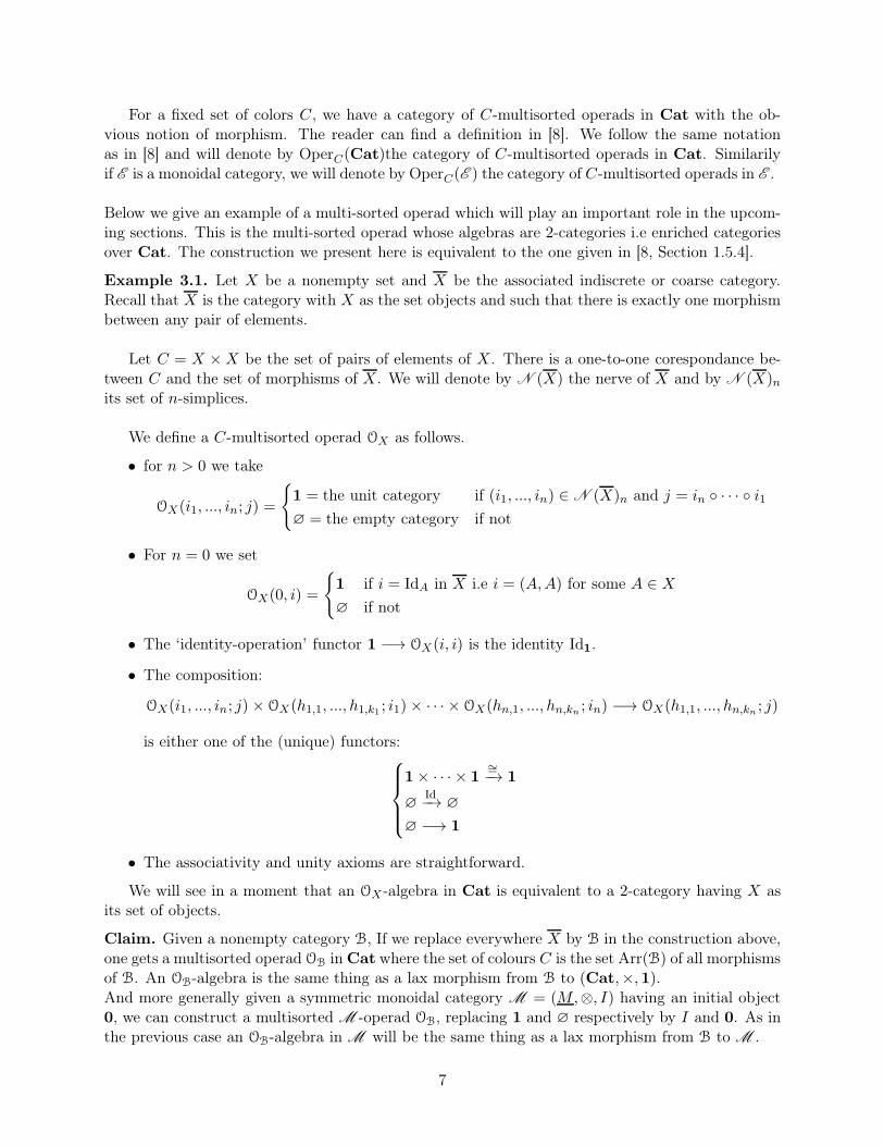
We define a C-multisorted operad OX as follows.

• for n > 0 we take

OX(i1, ..., in; j) =

{1 = the unit category if (i1, ..., in) ∈ N (X)n and j = in ◦ · · · ◦ i1

∅ = the empty category if not

• For n = 0 we set

OX(0, i) =

{1 if i = IdA in X i.e i = (A,A) for some A ∈ X

∅ if not

• The ‘identity-operation’ functor 1 −→ OX(i, i) is the identity Id1.

• The composition:

OX(i1, ..., in; j) × OX(h1,1, ..., h1,k1 ; i1)× · · · × OX(hn,1, ..., hn,kn ; in) −→ OX(h1,1, ..., hn,kn ; j)

is either one of the (unique) functors:

1× · · · × 1∼=−→ 1

∅Id−→ ∅

∅ −→ 1

• The associativity and unity axioms are straightforward.

We will see in a moment that an OX -algebra in Cat is equivalent to a 2-category having X asits set of objects.

Claim. Given a nonempty category B, If we replace everywhere X by B in the construction above,one gets a multisorted operad OB in Cat where the set of colours C is the set Arr(B) of all morphismsof B. An OB-algebra is the same thing as a lax morphism from B to (Cat,×,1).And more generally given a symmetric monoidal category M = (M,⊗, I) having an initial object0, we can construct a multisorted M -operad OB, replacing 1 and ∅ respectively by I and 0. As inthe previous case an OB-algebra in M will be the same thing as a lax morphism from B to M .

7

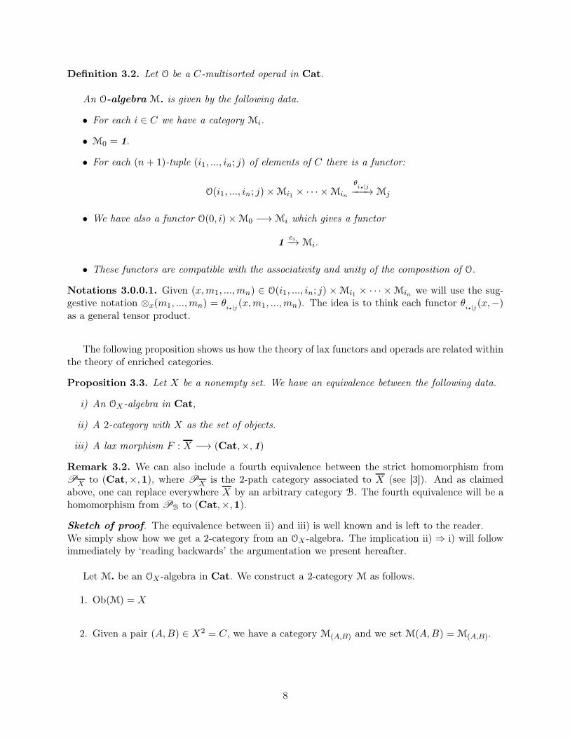
Definition 3.2. Let O be a C-multisorted operad in Cat.

An O-algebra M. is given by the following data.

• For each i ∈ C we have a category Mi.

• M0 = 1.

• For each (n + 1)-tuple (i1, ..., in; j) of elements of C there is a functor:

O(i1, ..., in; j) ×Mi1 × · · · ×Min

θi.|j−−−→Mj

• We have also a functor O(0, i) ×M0 −→Mi which gives a functor

1ei−→Mi.

• These functors are compatible with the associativity and unity of the composition of O.

Notations 3.0.0.1. Given (x,m1, ...,mn) ∈ O(i1, ..., in; j) ×Mi1 × · · · ×Min we will use the sug-gestive notation ⊗x(m1, ...,mn) = θ

i.|j (x,m1, ...,mn). The idea is to think each functor θi.|j(x,−)

as a general tensor product.

The following proposition shows us how the theory of lax functors and operads are related withinthe theory of enriched categories.

Proposition 3.3. Let X be a nonempty set. We have an equivalence between the following data.

i) An OX -algebra in Cat,

ii) A 2-category with X as the set of objects.

iii) A lax morphism F : X −→ (Cat,×,1)

Remark 3.2. We can also include a fourth equivalence between the strict homomorphism fromPX to (Cat,×,1), where PX is the 2-path category associated to X (see [3]). And as claimedabove, one can replace everywhere X by an arbitrary category B. The fourth equivalence will be ahomomorphism from PB to (Cat,×,1).

Sketch of proof. The equivalence between ii) and iii) is well known and is left to the reader.We simply show how we get a 2-category from an OX -algebra. The implication ii)⇒ i) will followimmediately by ‘reading backwards’ the argumentation we present hereafter.

Let M. be an OX -algebra in Cat. We construct a 2-category M as follows.

1. Ob(M) = X

2. Given a pair (A,B) ∈ X2 = C, we have a category M(A,B) and we set M(A,B) = M(A,B).

8

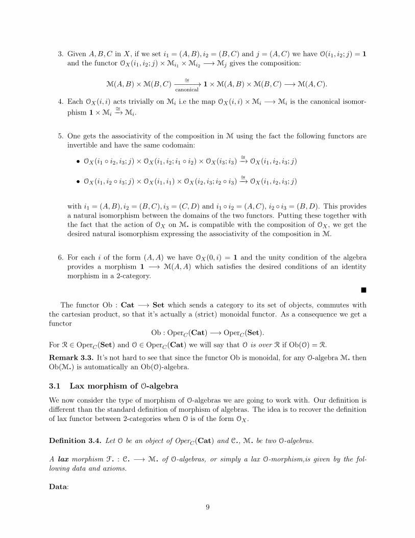
3. Given A,B,C in X, if we set i1 = (A,B), i2 = (B,C) and j = (A,C) we have O(i1, i2; j) = 1and the functor OX(i1, i2; j)×Mi1 ×Mi2 −→Mj gives the composition:

M(A,B)×M(B,C)∼=

−−−−−→canonical

1×M(A,B)×M(B,C) −→M(A,C).

4. Each OX(i, i) acts trivially on Mi i.e the map OX(i, i) ×Mi −→ Mi is the canonical isomor-

phism 1×Mi∼=−→Mi.

5. One gets the associativity of the composition in M using the fact the following functors areinvertible and have the same codomain:

• OX(i1 ◦ i2, i3; j)× OX(i1, i2; i1 ◦ i2)× OX(i3; i3)∼=−→ OX(i1, i2, i3; j)

• OX(i1, i2 ◦ i3; j)× OX(i1, i1)× OX(i2, i3; i2 ◦ i3)∼=−→ OX(i1, i2, i3; j)

with i1 = (A,B), i2 = (B,C), i3 = (C,D) and i1 ◦ i2 = (A,C), i2 ◦ i3 = (B,D). This providesa natural isomorphism between the domains of the two functors. Putting these together withthe fact that the action of OX on M. is compatible with the composition of OX , we get thedesired natural isomorphism expressing the associativity of the composition in M.

6. For each i of the form (A,A) we have OX(0, i) = 1 and the unity condition of the algebraprovides a morphism 1 −→ M(A,A) which satisfies the desired conditions of an identitymorphism in a 2-category.

�

The functor Ob : Cat −→ Set which sends a category to its set of objects, commutes withthe cartesian product, so that it’s actually a (strict) monoidal functor. As a consequence we get afunctor

Ob : OperC(Cat) −→ OperC(Set).

For R ∈ OperC(Set) and O ∈ OperC(Cat) we will say that O is over R if Ob(O) = R.

Remark 3.3. It’s not hard to see that since the functor Ob is monoidal, for any O-algebra M. thenOb(M.) is automatically an Ob(O)-algebra.

3.1 Lax morphism of O-algebra

We now consider the type of morphism of O-algebras we are going to work with. Our definition isdifferent than the standard definition of morphism of algebras. The idea is to recover the definitionof lax functor between 2-categories when O is of the form OX .

Definition 3.4. Let O be an object of OperC(Cat) and C., M. be two O-algebras.

A lax morphism F. : C. −→ M. of O-algebras, or simply a lax O-morphism,is given by the fol-lowing data and axioms.

Data:

9

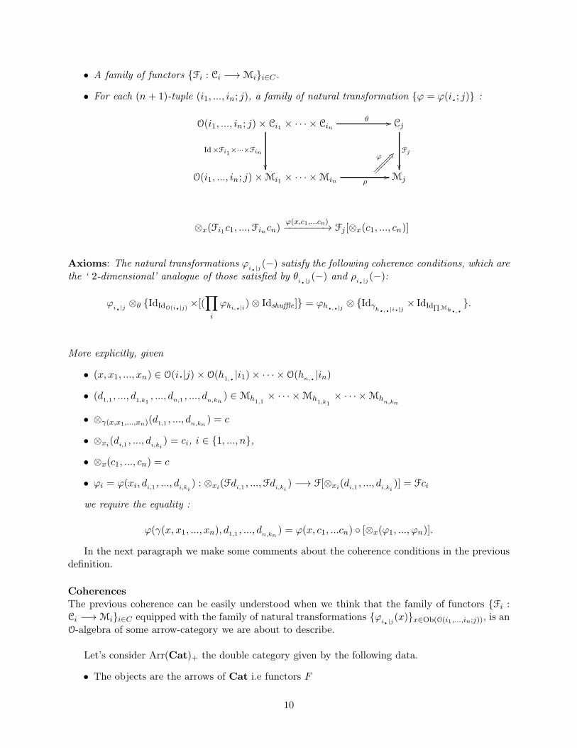
• A family of functors {Fi : Ci −→Mi}i∈C .

• For each (n + 1)-tuple (i1, ..., in; j), a family of natural transformation {ϕ = ϕ(i.; j)} :

O(i1, ..., in; j)× Ci1 × · · · × Cin Cj

O(i1, ..., in; j) ×Mi1 × · · · ×Min Mj

θ //

ρ//

Fj

��

Id×Fi1×···×Fin

��ϕ

;C⑧⑧⑧⑧⑧⑧

⑧⑧⑧⑧⑧⑧

⊗x(Fi1c1, ...,Fincn)ϕ(x,c1,...cn)−−−−−−−→ Fj [⊗x(c1, ..., cn)]

Axioms: The natural transformations ϕi.|j(−) satisfy the following coherence conditions, which are

the ‘ 2-dimensional’ analogue of those satisfied by θi.|j(−) and ρ

i.|j(−):

ϕi.|j⊗θ {IdIdO(i.|j)

×[(∏

i

ϕhi,.|i)⊗ Idshuffle]} = ϕh.,.|j⊗ {Idγ

h.,.|i.|j

× IdId∏Mh.,.}.

More explicitly, given

• (x, x1, ..., xn) ∈ O(i.|j)× O(h1,. |i1)× · · · × O(hn,. |in)

• (d1,1 , ..., d1,k1, ..., dn,1 , ..., dn,kn

) ∈Mh1,1× · · · ×Mh

1,k1× · · · ×Mh

n,kn

• ⊗γ(x,x1,...,xn)(d1,1 , ..., dn,kn) = c

• ⊗xi(di,1 , ..., di,ki) = ci, i ∈ {1, ..., n},

• ⊗x(c1, ..., cn) = c

• ϕi = ϕ(xi, di,1 , ..., di,ki) : ⊗xi(Fdi,1 , ...,Fdi,ki

) −→ F[⊗xi(di,1 , ..., di,ki)] = Fci

we require the equality :

ϕ(γ(x, x1, ..., xn), d1,1 , ..., dn,kn) = ϕ(x, c1, ...cn) ◦ [⊗x(ϕ1, ..., ϕn)].

In the next paragraph we make some comments about the coherence conditions in the previousdefinition.

CoherencesThe previous coherence can be easily understood when we think that the family of functors {Fi :Ci −→Mi}i∈C equipped with the family of natural transformations {ϕ

i. |j(x)}x∈Ob(O(i1,...,in;j)), is anO-algebra of some arrow-category we are about to describe.

Let’s consider Arr(Cat)+ the double category given by the following data.

• The objects are the arrows of Cat i.e functors F

10

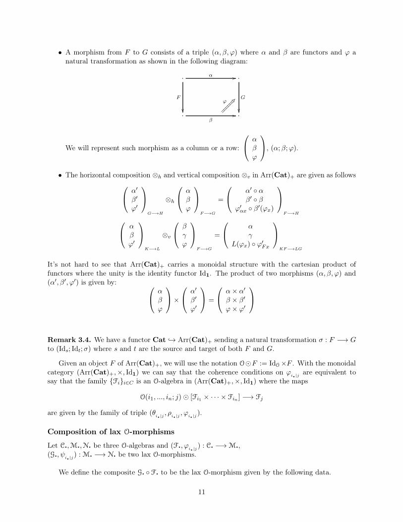
• A morphism from F to G consists of a triple (α, β, ϕ) where α and β are functors and ϕ anatural transformation as shown in the following diagram:

· ·

· ·

α //

β//

G

��

F

��

ϕ;C

⑧⑧⑧⑧⑧⑧

⑧⑧⑧⑧⑧⑧

We will represent such morphism as a column or a row:

αβϕ

, (α;β;ϕ).

• The horizontal composition ⊗h and vertical composition ⊗v in Arr(Cat)+ are given as follows

α′

β′

ϕ′

G−→H

⊗h

αβϕ

F−→G

=

α′ ◦ αβ′ ◦ β

ϕ′αx ◦ β

′(ϕx)

F−→H

αβϕ′

K−→L

⊗v

βγϕ

F−→G

=

αγ

L(ϕx) ◦ ϕ′Fx

KF−→LG

It’s not hard to see that Arr(Cat)+ carries a monoidal structure with the cartesian product offunctors where the unity is the identity functor Id1. The product of two morphisms (α, β, ϕ) and(α′, β′, ϕ′) is given by:

αβϕ

×

α′

β′

ϕ′

=

α× α′

β × β′

ϕ× ϕ′

Remark 3.4. We have a functor Cat → Arr(Cat)+ sending a natural transformation σ : F −→ Gto (Ids; Idt;σ) where s and t are the source and target of both F and G.

Given an object F of Arr(Cat)+, we will use the notation O⊙F := IdO×F . With the monoidalcategory (Arr(Cat)+,×, Id1) we can say that the coherence conditions on ϕ

i.|j are equivalent tosay that the family {Fi}i∈C is an O-algebra in (Arr(Cat)+,×, Id1) where the maps

O(i1, ..., in; j) ⊙ [Fi1 × · · · × Fin ] −→ Fj

are given by the family of triple (θi.|j , ρi.|j , ϕi.|j ).

Composition of lax O-morphisms

Let C.,M.,N. be three O-algebras and (F., ϕi.|j ) : C. −→M.,

(G., ψi. |j) : M. −→ N. be two lax O-morphisms.

We define the composite G. ◦ F. to be the lax O-morphism given by the following data.

11

• The family of functors {Gi ◦ Fi : Ci −→ Ni}i∈C .

• For each (n+1)-tuple (i1, ..., in; j), the family of natural transformation {χi.|j (x)}x∈Ob(O(i1,...,in;j))

where:χ

i.|j (x) = Gj [ϕi. |j(x)] ◦ ψi.|j(x)∏Fi(−).

• More precisely the component of χi.|j (x) at (c1, ..., cn) ∈ Ci1 × · · · × Cin is the morphism:

χi.|j (x)(c1,...,cn) = Gj [ϕi.|j (x)(c1,...,cn)] ◦ ψi.|j(x)(Fi1

c1,...,Fincn).

We leave the reader to check that these data satisfy the coherence conditions of the Definition 3.4.

Remark 3.5.The identity O-morphims of an algebra (M., θ

i.|j ) is given by the family of functors {IdMi}i∈C and

natural transformations {Idθi.|j (x)

}x∈Ob(O(i1,...,in;j)).

3.2 Morphisms of lax O-morphisms

O-algebras and lax O-morphisms form naturally a category. But there is an obvious notion of2-morphism we now describe. A 2-morphism is the analogue of the transformations of lax functors.

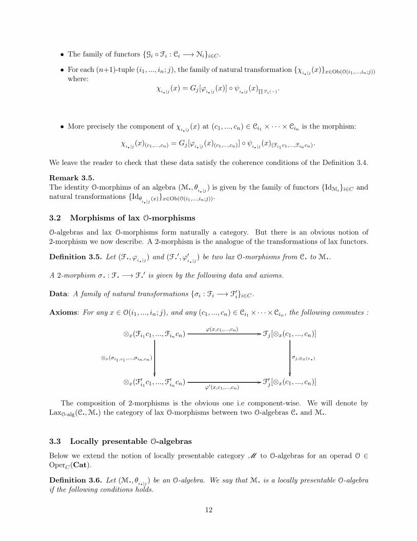
Definition 3.5. Let (F., ϕi.|j) and (F.′, ϕ′

i.|j) be two lax O-morphisms from C. to M..

A 2-morphism σ. : F. −→ F.′ is given by the following data and axioms.

Data: A family of natural transformations {σi : Fi −→ F′i}i∈C .

Axioms: For any x ∈ O(i1, ..., in; j), and any (c1, ..., cn) ∈ Ci1 ×· · ·×Cin, the following commutes :

⊗x(Fi1c1, ...,Fincn) Fj [⊗x(c1, ..., cn)]

⊗x(F′i1c1, ...,F

′incn) F′

j [⊗x(c1, ..., cn)]

ϕ(x,c1,...,cn) //

ϕ′(x,c1,...,cn)//

σj,⊗x(c.)

��

⊗x(σi1,c1 ,...,σin,cn)

��

The composition of 2-morphisms is the obvious one i.e component-wise. We will denote byLaxO-alg(C.,M.) the category of lax O-morphisms between two O-algebras C. and M..

3.3 Locally presentable O-algebras

Below we extend the notion of locally presentable category M to O-algebras for an operad O ∈OperC(Cat).

Definition 3.6. Let (M., θi.|j

) be an O-algebra. We say that M. is a locally presentable O-algebraif the following conditions holds.

12

• For every i ∈ C the category Mi is a locally presentable category in the usual sense.

• For every (i1, ..., in; j) the functor θi.|j

preserves the colimits on each factor ‘ik’ (1 ≤ k ≤ n)that is for every (ml)l 6=k ∈

∏l,l 6=kMil and every x ∈ O(i1, ..., in; j) the functor

θi.|j

(x; (ml)) := θi.|j

(x; ...,ml, ...mk−1,−,mk+1, ...) : Mik −→Mj

preserves all colimits.

Example 3.7.

1. If O is the operad of enriched categories, then any symmetric closed monoidal category M

which is locally presentable is automatically a locally presentable O-algebra. The secondcondition of the definition follows from the fact that being closed monoidal imply that thetensor product of M (which is a left adjoint) preserves colimits on each factor.

2. More generally any biclosed monoidal category M (see [20, 1.5]), not necessarily symmetric,which is locally presentable is a locally presentable O-algebra.

3. Any 2-category (or bicategory) such that the composition preserves the colimits on each factorand all the category of morphisms are locally presentable, is a locally presentable OX -algebrafor the operad OX of the Example 3.1.

Remark 3.6. In the same fashion way we will say that M. is a cocomplete O-algebra if all the Mi

are cocomplete and if the second condition of the previous definition holds.

The main result in this section is the following.

Theorem 3.8. Let M. be a locally presentable O-algebra. For any O-algebra C. the category of laxO-morphisms LaxO-alg(C.,M.) is locally presentable.

Proof. See Appendix D �

3.4 Special Quillen O-algebra

In the following we consider an ad-hoc notion of Quillen O-algebra.

Definition 3.9. Let (M., θi.|j

) be an O-algebra. We say that M. is a special Quillen O-algebra

if the following conditions holds.

1. M. is complete and cocomplete,

2. For every i ∈ C the category Mi is a Quillen closed model category in the usual sense.

3. For every x ∈ O(i1, ..., in; j), the functor ⊗x preserves (trivial) cofibrations with cofibrantdomain. This means that for every n-tuple of morphisms (gk)k in Mi1 × · · · × Min , suchthat each gk has a cofibrant domain, then ⊗x(g1, ..., gn) is a (trivial) cofibration in Mj if allg1, ..., gn are (trivial) cofibrations.

Say that M. is cofibrantly generated if all the Mi are cofibrantly generated. Similarly if each Mi iscombinatorial we will say that M. is combinatorial.

Example 3.10.

13

• Any model category is obviously a special Quillen O-algebra with the tautological operad (nooperations except the 1-ary identity operation).

• Another example of special Quillen algebra is a symmetric monoidal model category. In factusing the pushout-product axiom one has that (trivial) cofibrations with cofibrant domain areclosed by tensor product.

Remark 3.7. Note that in our definition we did not include a generalized pushout product axiom;it doesn’t seem relevant, for our purposes, to impose this axioms in general. But if one is interestedof having such axiom, a first approximation will be of course to mimic the monoidal situation. Belowwe give a sketchy one.

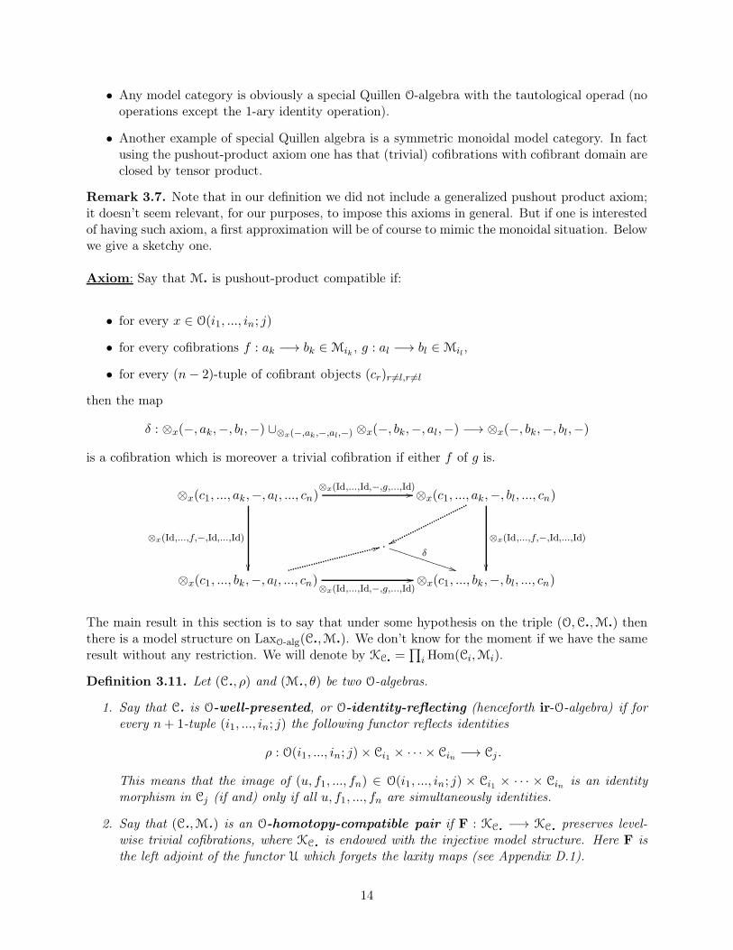
Axiom: Say that M. is pushout-product compatible if:

• for every x ∈ O(i1, ..., in; j)

• for every cofibrations f : ak −→ bk ∈Mik , g : al −→ bl ∈Mil ,

• for every (n− 2)-tuple of cofibrant objects (cr)r 6=l,r 6=l

then the map

δ : ⊗x(−, ak,−, bl,−) ∪⊗x(−,ak ,−,al,−) ⊗x(−, bk,−, al,−) −→ ⊗x(−, bk,−, bl,−)

is a cofibration which is moreover a trivial cofibration if either f of g is.

⊗x(c1, ..., ak,−, al, ..., cn) ⊗x(c1, ..., ak,−, bl, ..., cn)

⊗x(c1, ..., bk,−, al, ..., cn) ⊗x(c1, ..., bk,−, bl, ..., cn)

⊗x(Id,...,Id,−,g,...,Id)//

⊗x(Id,...,Id,−,g,...,Id)//

⊗x(Id,...,f,−,Id,...,Id)

��

⊗x(Id,...,f,−,Id,...,Id)

��

. ww33δ

**❚❚❚❚❚❚

❚❚❚❚❚❚

The main result in this section is to say that under some hypothesis on the triple (O,C.,M.) thenthere is a model structure on LaxO-alg(C.,M.). We don’t know for the moment if we have the sameresult without any restriction. We will denote by KC. =

∏iHom(Ci,Mi).

Definition 3.11. Let (C., ρ) and (M., θ) be two O-algebras.

1. Say that C. is O-well-presented, or O-identity-reflecting (henceforth ir-O-algebra) if forevery n+ 1-tuple (i1, ..., in; j) the following functor reflects identities

ρ : O(i1, ..., in; j)× Ci1 × · · · × Cin −→ Cj .

This means that the image of (u, f1, ..., fn) ∈ O(i1, ..., in; j) × Ci1 × · · · × Cin is an identitymorphism in Cj (if and) only if all u, f1, ..., fn are simultaneously identities.

2. Say that (C.,M.) is an O-homotopy-compatible pair if F : KC. −→ KC. preserves level-wise trivial cofibrations, where KC. is endowed with the injective model structure. Here F isthe left adjoint of the functor U which forgets the laxity maps (see Appendix D.1).

14

The motivation of these definitions is explained in the Appendix E.With the previous material we have

Theorem 3.12. For an ir-O-algebra C., and a special Quillen O-algebra M. assume that

• (C.,M.) is an O-homotopy compatible pair,

• all objects of M. are cofibrant,

• M is cofibrantly generated with I. (resp. J.) the generating set of (trivial) cofibrations

then there is a model structure on LaxO-alg(C.,M.) which is cofibrantly generated. A map σ : F −→ G

is

• a weak equivalence if Uσ is a weak equivalence in KC.,

• a fibration if Uσ is a fibration in KC.,

• a cofibration if it has the LLP with respect to all maps which are both fibrations and weakequivalences,

• a trivial cofibration if it has the LLP with respect to all fibrations.

• the set F(I.) and F(J.) constitute respectively the set of generating cofibrations and trivialcofibrations in LaxO-alg(C.,M.).

The pair

U : LaxO-alg(C.,M.)⇆∏

i

Hom(Ci,Mi) : F

is a Quillen pair, where F is left Quillen and U right Quillen.

Proof. The idea is to transfer the (product) model structure on KC. =∏iHom(Ci,Mi) through

the monadic adjunction F ⊣ U using a lemma of Schwede-Shipley [34]. In fact LaxO-alg(C.,M.) isequivalent to T-alg for the monad T = UF. The method is exactly the same as in the proof oftheorem 7.6.All we have to check is that the pushout of Fσ is a weak equivalence for every generating trivialcofibration σ in KC.. This is exposed in the Appendix E. �

An alternative description of LaxO-alg(C.,M.)

In the following we fix a multi-sorted operad O and an O-algebra C.. Our goal is to describe thecategory LaxO-alg(C.,M.) as subcategory of LaxO’-alg(1.,M.) for some operad O′ = OC. =

∫C.; here

1. is the terminal algebra. This will simplify many construction such as pushouts and colimit ingeneral.

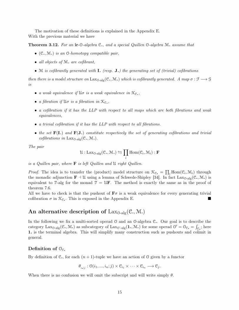
Definition of OC.

By definition of C., for each (n+ 1)-tuple we have an action of O given by a functor

θi.|j : O(i1, ..., in; j) × Ci1 × · · · × Cin −→ Cj.

When there is no confusion we will omit the subscript and will write simply θ.

15

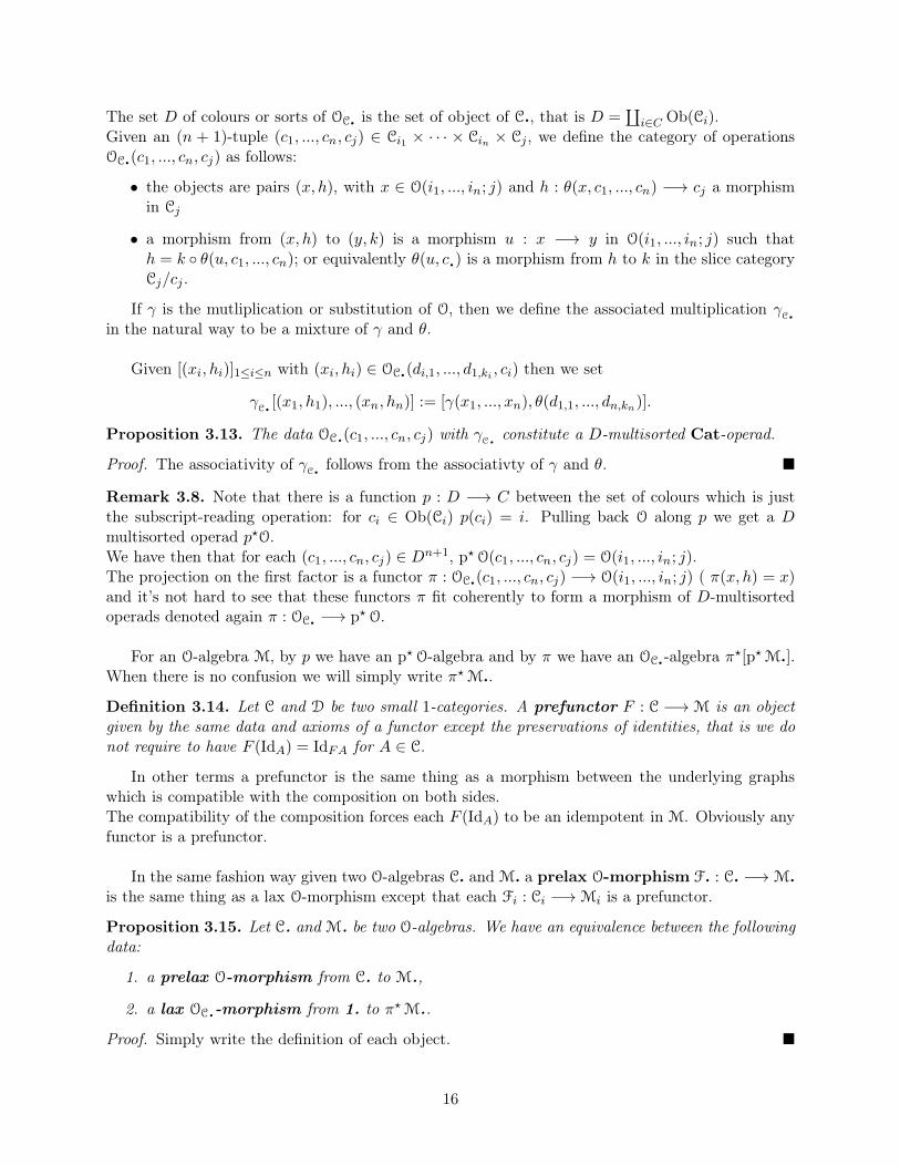
The set D of colours or sorts of OC. is the set of object of C., that is D =∐i∈C Ob(Ci).

Given an (n + 1)-tuple (c1, ..., cn, cj) ∈ Ci1 × · · · × Cin × Cj, we define the category of operationsOC.(c1, ..., cn, cj) as follows:

• the objects are pairs (x, h), with x ∈ O(i1, ..., in; j) and h : θ(x, c1, ..., cn) −→ cj a morphismin Cj

• a morphism from (x, h) to (y, k) is a morphism u : x −→ y in O(i1, ..., in; j) such thath = k ◦ θ(u, c1, ..., cn); or equivalently θ(u, c.) is a morphism from h to k in the slice categoryCj/cj .

If γ is the mutliplication or substitution of O, then we define the associated multiplication γC.

in the natural way to be a mixture of γ and θ.

Given [(xi, hi)]1≤i≤n with (xi, hi) ∈ OC.(di,1, ..., d1,ki , ci) then we set

γC. [(x1, h1), ..., (xn, hn)] := [γ(x1, ..., xn), θ(d1,1, ..., dn,kn)].

Proposition 3.13. The data OC.(c1, ..., cn, cj) with γC.

constitute a D-multisorted Cat-operad.

Proof. The associativity of γC. follows from the associativty of γ and θ. �

Remark 3.8. Note that there is a function p : D −→ C between the set of colours which is justthe subscript-reading operation: for ci ∈ Ob(Ci) p(ci) = i. Pulling back O along p we get a Dmultisorted operad p⋆O.We have then that for each (c1, ..., cn, cj) ∈ D

n+1, p⋆O(c1, ..., cn, cj) = O(i1, ..., in; j).The projection on the first factor is a functor π : OC.(c1, ..., cn, cj) −→ O(i1, ..., in; j) ( π(x, h) = x)and it’s not hard to see that these functors π fit coherently to form a morphism of D-multisortedoperads denoted again π : OC. −→ p⋆ O.

For an O-algebra M, by p we have an p⋆ O-algebra and by π we have an OC.-algebra π⋆[p⋆M.].When there is no confusion we will simply write π⋆M..

Definition 3.14. Let C and D be two small 1-categories. A prefunctor F : C −→M is an objectgiven by the same data and axioms of a functor except the preservations of identities, that is we donot require to have F (IdA) = IdFA for A ∈ C.

In other terms a prefunctor is the same thing as a morphism between the underlying graphswhich is compatible with the composition on both sides.The compatibility of the composition forces each F (IdA) to be an idempotent in M. Obviously anyfunctor is a prefunctor.

In the same fashion way given two O-algebras C. and M. a prelax O-morphism F. : C. −→M.is the same thing as a lax O-morphism except that each Fi : Ci −→Mi is a prefunctor.

Proposition 3.15. Let C. and M. be two O-algebras. We have an equivalence between the followingdata:

1. a prelax O-morphism from C. to M.,

2. a lax OC.-morphism from 1. to π⋆M..

Proof. Simply write the definition of each object. �

16

4 Co-Segal Categories

4.1 The one-object case

Conventions.

• By semi-monoidal category we mean the same structure as a monoidal category exceptthat no unit object is required. Obviously any monoidal category has an underlying semi-monoidal category.

• A lax functor between semi-monoidal categories is the same thing as a lax functor betweenmonoidal categories without the data involving the units. A strict lax functor will be call aswell ‘monoidal functor’.

• More generally we will say semi-bicategory (resp. semi-2-category) to be the same thing asbicategory (resp. 2-category) except that we don’t require the identities 1-morphisms.

• We have also the notion of lax morphism, transformation of lax morphisms, between semi-bicategories in the natural way.

• For a semi-bicategory A and a bicategory B, a lax morphism from A to B will be a morphismfrom A to the underlying semi-bicategory of B which will be denoted again B.

In the following we fix M = (M,⊗, I) a monoidal category.

4.2 Overview

As we identify M -categories with one object and monoids of M , we shall expect that a Co-Segal category with one object will be a kind of homotopical semi-monoid1 of M . We will call themCo-Segal semi-monoids.

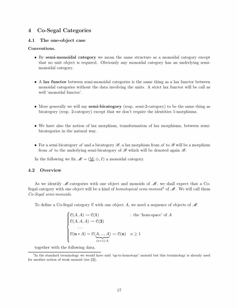
To define a Co-Segal category C with one object A, we need a sequence of objects of M

C(A,A) C(1) : the ‘hom-space’ of A

C(A,A,A) C(2)

· · ·

C(n ∗ A) = C(A, ..., A︸ ︷︷ ︸(n+1)-A

) C(n) n ≥ 1

together with the following data.

1In the standard terminology we would have said ‘up-to-homotopy’ monoid but this terminology is already usedfor another notion of weak monoid (see [3]).

17

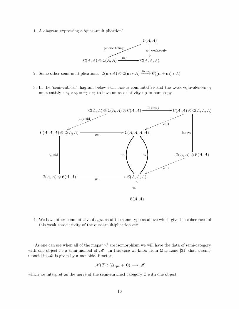
1. A diagram expressing a ‘quasi-multiplication’

C(A,A) ⊗ C(A,A) C(A,A,A)

C(A,A)

µ1,1 //

weak.equivγ0

��

generic lifting

55

2. Some other semi-multiplications: C(n ∗A)⊗ C(m ∗ A)µn,m−−−→ C((n + m) ∗ A)

3. In the ‘semi-cubical’ diagram below each face is commutative and the weak equivalences γimust satisfy : γ1 ◦ γ0 = γ2 ◦ γ0 to have an associativity up-to homotopy.

C(A,A)⊗ C(A,A) ⊗ C(A,A) C(A,A)⊗ C(A,A,A)

C(A,A,A) ⊗ C(A,A) C(A,A,A,A)

Id⊗µ1,1 //

µ1,1⊗Id

uu❧❧❧❧❧❧

❧❧❧❧❧❧

❧❧❧❧❧❧

❧❧❧❧

µ1,2

uu❧❧❧❧❧❧

❧❧❧❧❧❧

❧❧❧❧❧❧

❧❧❧❧

µ2,1//

C(A,A) ⊗ C(A,A)

C(A,A) ⊗ C(A,A) C(A,A,A)

µ1,1

uu❧❧❧❧❧❧

❧❧❧❧❧❧

❧❧❧❧❧❧

❧❧❧❧

γ0⊗Id

OOId⊗γ0

OO

µ1,1//

γ2

\\

γ1

BB

C(A,A)

γ0

OO

4. We have other commutative diagrams of the same type as above which give the coherences ofthis weak associativity of the quasi-multiplication etc.

As one can see when all of the maps ‘γi’ are isomorphism we will have the data of semi-categorywith one object i.e a semi-monoid of M . In this case we know from Mac Lane [31] that a semi-monoid in M is given by a monoidal functor:

N (C) : (∆epi,+,0) −→M

which we interpret as the nerve of the semi-enriched category C with one object.

18

Remark 4.1. The object 0 doesn’t play any role here since there is no morphism from any anotherobject to it. So we can restrict this functor to the underlyinng semi-monoidal categories (seeDefinition 4.2 below).

4.3 Definitions

Notations 4.3.0.2.

• We will denote by n the set {0, · · · , n− 1} with the natural order on it.

• The objects of ∆ will be identified with those n and the morphisms will be the nondecreasingfunctions. The object 0 corresponds to the empty set.

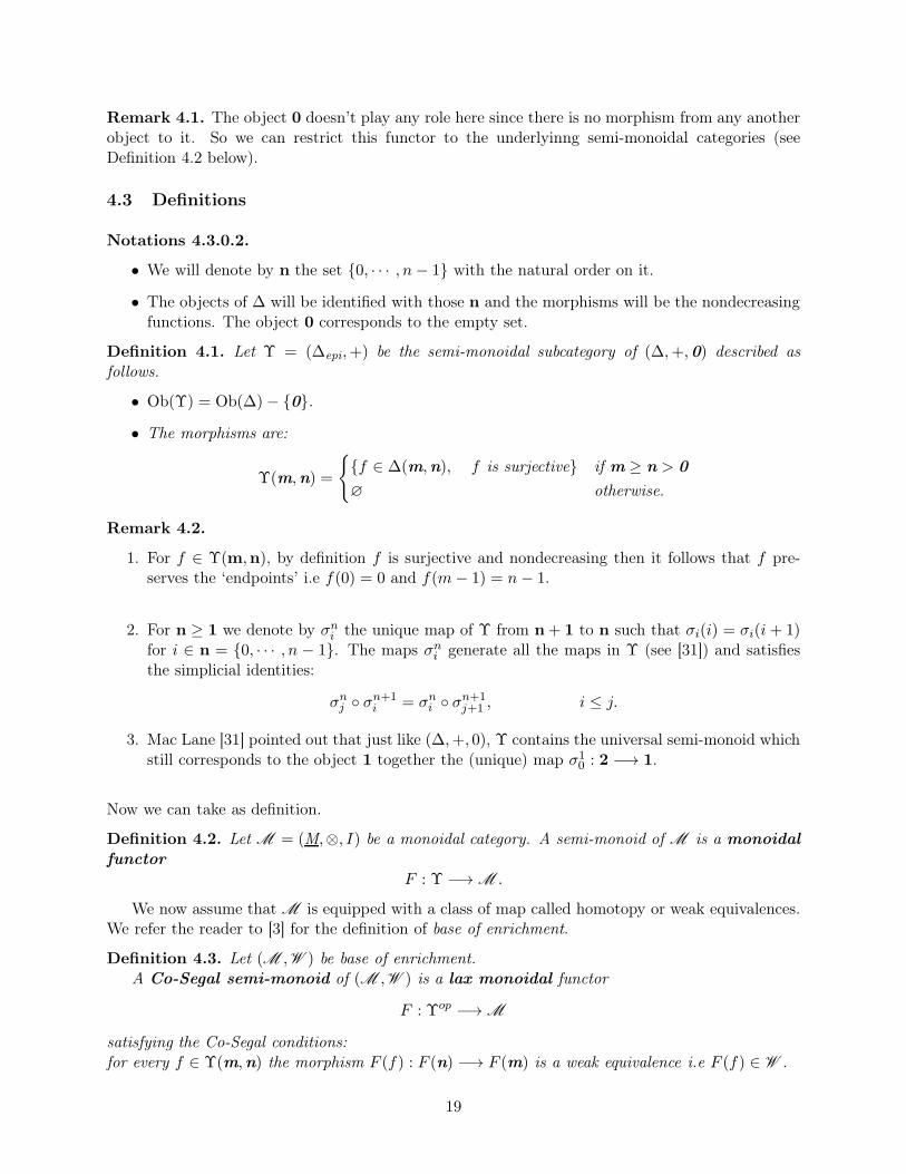
Definition 4.1. Let Υ = (∆epi,+) be the semi-monoidal subcategory of (∆,+,0) described asfollows.

• Ob(Υ) = Ob(∆)− {0}.

• The morphisms are:

Υ(m,n) =

{{f ∈ ∆(m,n), f is surjective} if m ≥ n > 0

∅ otherwise.

Remark 4.2.

1. For f ∈ Υ(m,n), by definition f is surjective and nondecreasing then it follows that f pre-serves the ‘endpoints’ i.e f(0) = 0 and f(m− 1) = n− 1.

2. For n ≥ 1 we denote by σni the unique map of Υ from n + 1 to n such that σi(i) = σi(i+ 1)for i ∈ n = {0, · · · , n − 1}. The maps σni generate all the maps in Υ (see [31]) and satisfiesthe simplicial identities:

σnj ◦ σn+1i = σni ◦ σ

n+1j+1 , i ≤ j.

3. Mac Lane [31] pointed out that just like (∆,+, 0), Υ contains the universal semi-monoid whichstill corresponds to the object 1 together the (unique) map σ10 : 2 −→ 1.

Now we can take as definition.

Definition 4.2. Let M = (M,⊗, I) be a monoidal category. A semi-monoid of M is a monoidal

functor

F : Υ −→M .

We now assume that M is equipped with a class of map called homotopy or weak equivalences.We refer the reader to [3] for the definition of base of enrichment.

Definition 4.3. Let (M ,W ) be base of enrichment.A Co-Segal semi-monoid of (M ,W ) is a lax monoidal functor

F : Υop −→M

satisfying the Co-Segal conditions:for every f ∈ Υ(m,n) the morphism F (f) : F (n) −→ F (m) is a weak equivalence i.e F (f) ∈ W .

19

Remark 4.3.

1. It’s important to notice that in the first definition we use Υ = (∆epi,+) while in the secondwe use Υop = (∆epi

op,+).

2. Here as usual, the underlying semi-monoid is the object F (1).

3. Finally it’s important to notice that since the morphism of Υ are generated by the maps σniand because W is stable by composition, it suffices to require the Co-Segal conditions onlyfor the maps F (σni ).

To understand the definition one needs to see the data that F carries.

Observations 1.

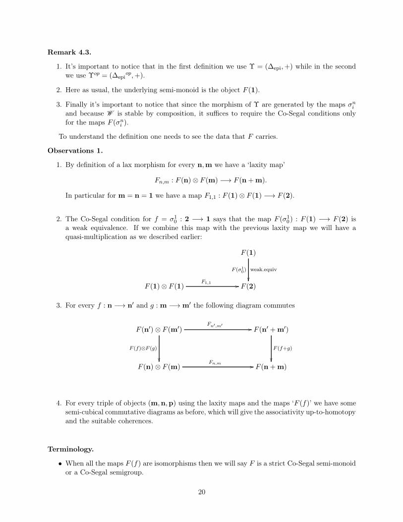
1. By definition of a lax morphism for every n,m we have a ‘laxity map’

Fn,m : F (n)⊗ F (m) −→ F (n + m).

In particular for m = n = 1 we have a map F1,1 : F (1)⊗ F (1) −→ F (2).

2. The Co-Segal condition for f = σ10 : 2 −→ 1 says that the map F (σ10) : F (1) −→ F (2) isa weak equivalence. If we combine this map with the previous laxity map we will have aquasi-multiplication as we described earlier:

F (1)⊗ F (1) F (2)

F (1)

F1,1 //

weak.equivF (σ10)

��

3. For every f : n −→ n′ and g : m −→m′ the following diagram commutes

F (n′)⊗ F (m′) F (n′ + m′)

F (n)⊗ F (m) F (n + m)

Fn′,m′//

F (f)⊗F (g)

��

F (f+g)

��Fn,m //

4. For every triple of objects (m,n,p) using the laxity maps and the maps ‘F (f)’ we have somesemi-cubical commutative diagrams as before, which will give the associativity up-to-homotopyand the suitable coherences.

Terminology.

• When all the maps F (f) are isomorphisms then we will say F is a strict Co-Segal semi-monoidor a Co-Segal semigroup.

20

• Without the Co-Segal conditions in the Definition 4.3 we will say that F is a pre-semi-monoid.

Proposition 4.4. We have an equivalence between the following data:

• a classical semi-monoid or semigroup of M

• a strict Co-Segal semi-monoid of M .

When we will define the morphisms between Co-Segal semi-monoids, this equivalence will auto-matically be an equivalence of categories.

Sketch of proof.

a) Let F : Υ −→ M be a semi-monoid. We define the corresponding Co-Segal semi-monoid Fas follows.

• We set F (n) = F (1) := F (1) for every n, and for every f : m −→ n we set F (f) :=IdF (1).

• Finally the laxity maps correspond to the multiplication of the semi-monoid F (1) i.eFn,m is the composite:

F (1)⊗ F (1)Id−→ F (2)

F (σ10)−−−→ F (1)

for m ≥ 1,n ≥ 1.

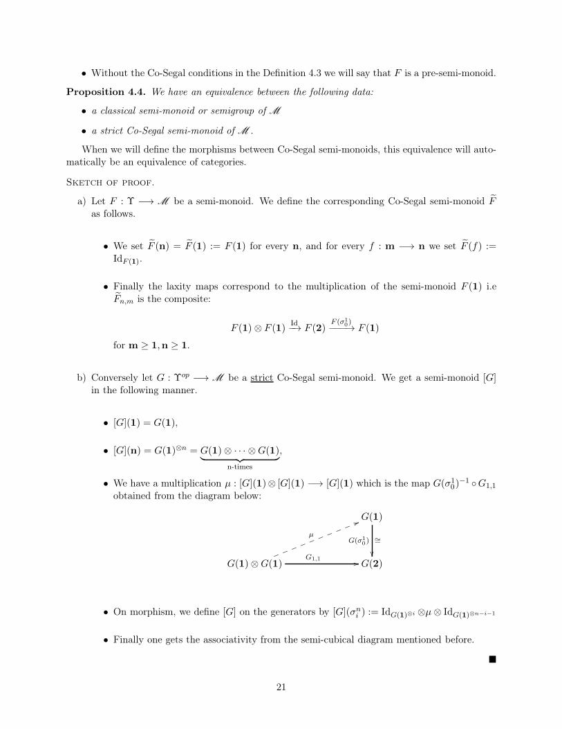
b) Conversely let G : Υop −→M be a strict Co-Segal semi-monoid. We get a semi-monoid [G]in the following manner.

• [G](1) = G(1),

• [G](n) = G(1)⊗n = G(1)⊗ · · · ⊗G(1)︸ ︷︷ ︸n-times

,

• We have a multiplication µ : [G](1)⊗ [G](1) −→ [G](1) which is the map G(σ10)−1 ◦G1,1

obtained from the diagram below:

G(1)⊗G(1) G(2)

G(1)

G1,1 //

∼=G(σ10)

��

µ

55❧❧❧❧❧❧❧❧❧❧

• On morphism, we define [G] on the generators by [G](σni ) := IdG(1)⊗i ⊗µ⊗ IdG(1)⊗n−i−1

• Finally one gets the associativity from the semi-cubical diagram mentioned before.

�

21

4.4 The General case: Co-Segal Categories

4.5 S-Diagrams

In addition to the notations of the previous section, we will also use the following ones.

Notations 4.5.0.3.Cat≤1 = the 1-category of small categories with functors.Bicat2= the 2-category of bicategories, lax morphisms and icons ([24, Thm 3.2]). 2

12 Bicat2 = the category of semi-bicategories, lax morphisms and icons.PC = the 2-path-category associated to a small category C (see [3]) .∆+ = the category ∆ without the object 0 i.e the category of finite nonempty ordinals.Υ+ = the category Υ without the object 0.

1 = {O,OIdO−−→ O} = the unit category.

X = the coarse category associated to a nonempty set X (see [3]).(B)2-op = the 2-opposite (semi) bicategory of B. We keep the same 1-cells but reverse the 2-cellsi.e

(B)2-op(A,B) := B(A,B)op.

(M ,W ) = a base of enrichment, with M is a general bicategory.2-Iso(M ) = the class of invertible 2-morphisms of M . Recall that (M , 2-Iso) is the smallest baseof enrichment.

Note. We will freely identify bicategories and 2-categories. And as usual monoidal categories willbe identified with bicategories with one object.

Recall that the 2-path category PC is a generalized version of the monoidal category (∆,+,0)in the sense that when C ∼= 1 then PC

∼= (∆,+,0). It has been shown in [3] that a classical enrichedcategory with a small set of objects was the same thing as a homomorphism in the sense of Bénaboufrom PX to M , for some set X.

In what follows we introduce a generalized version of the semi-monoidal category Υ = (∆epi,+)just like we did for (∆,+,0). For C a small category, we consider SC, a semi-2-category containedin PC, such that S1 ‘is’ Υ.

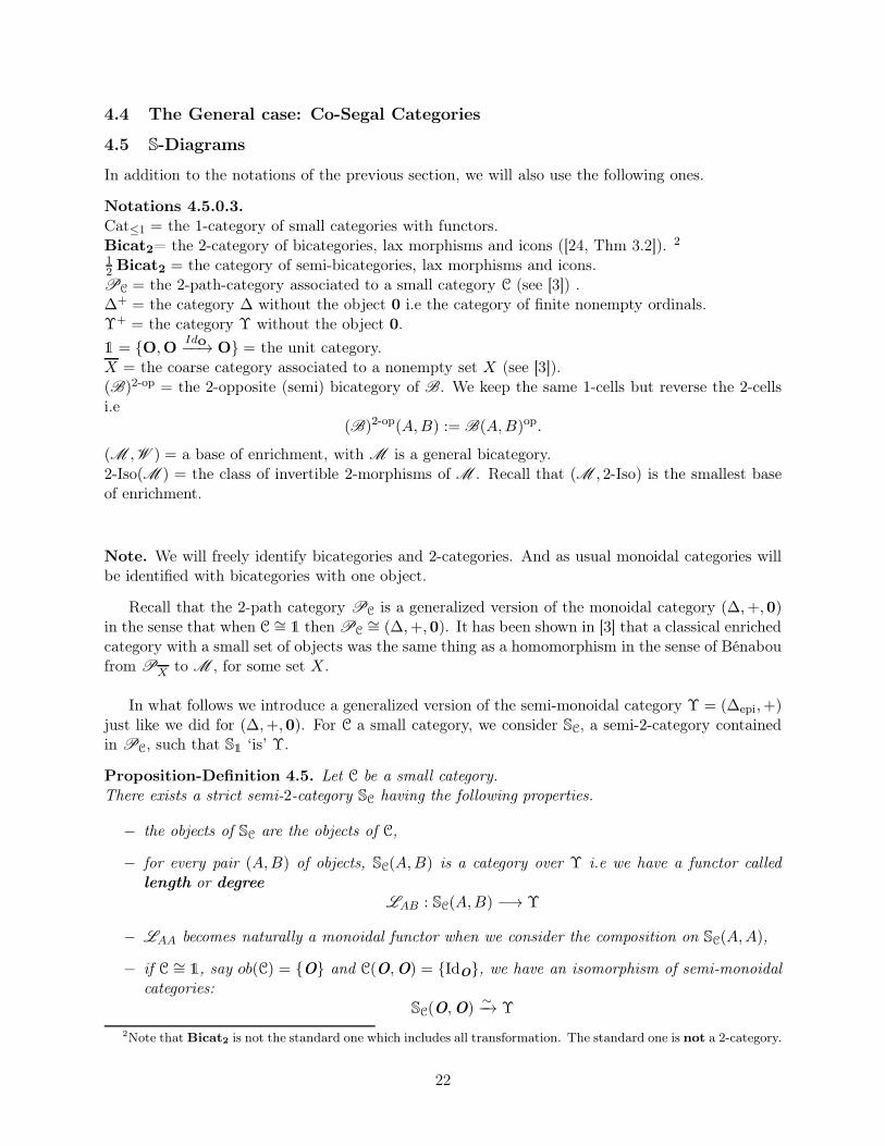
Proposition-Definition 4.5. Let C be a small category.There exists a strict semi-2-category SC having the following properties.

− the objects of SC are the objects of C,

− for every pair (A,B) of objects, SC(A,B) is a category over Υ i.e we have a functor calledlength or degree

LAB : SC(A,B) −→ Υ

− LAA becomes naturally a monoidal functor when we consider the composition on SC(A,A),

− if C ∼= 1, say ob(C) = {O} and C(O,O) = {IdO}, we have an isomorphism of semi-monoidalcategories:

SC(O,O)∼−→ Υ

2Note that Bicat2 is not the standard one which includes all transformation. The standard one is not a 2-category.

22

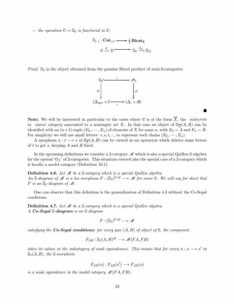
− the operation C 7→ SC is functorial in C:

S[−] : Cat≤112 Bicat2

CF−→ D SC

SF−−→ SD

//

✤ //

Proof. SC is the object obtained from the genuine fibred product of semi-2-categories:

SC PC

(∆epi,+) (∆,+,0)

� � i //

L

��� �

i//

L

��

�

Note. We will be interested in particular to the cases where C is of the form X, the indiscreteor coarse category associated to a nonempty set X. In that case an object of SX(A,B) can beidentified with an (n+1)-tuple (E0, · · · , En) of elements of X for some n, with E0 = A and En = B.For simplicity we will use small letters: r, s, t,..., to represent such chains (E0, · · · , En).

A morphism u : t −→ s of SX(A,B) can be viewed as an operation which deletes some lettersof t to get s, keeping A and B fixed.

In the upcoming definitions we consider a 2-category M which is also a special Quillen O-algebrafor the operad ‘OX ’ of 2-categories. This situation covered also the special case of a 2-category whichis locally a model category (Definition 10.1).

Definition 4.6. Let M be a 2-category which is a special Quillen algebra.An S-diagram of M is a lax morphism F : (SC)

2-op −→M for some C. We will say for short thatF is an SC-diagram of M .

One can observe that this definition is the generalization of Definition 4.3 without the Co-Segalconditions.

Definition 4.7. Let M be a 2-category which is a special Quillen algebra.A Co-Segal S-diagram is an S-diagram

F : (SC)2-op −→M

satisfying the Co-Segal conditions: for every pair (A,B) of object of C, the component

FAB : SC(A,B)op −→M (FA,FB)

takes its values in the subcategory of weak equivalences. This means that for every u : s −→ s′ inSC(A,B), the 2-morphism

FAB(u) : FAB(s′) −→ FAB(s)

is a weak equivalence in the model category M (FA,FB).

23

Terminology. When all the maps FAB(u) are 2-isomorphisms , then we will say that F is as strictCo-Segal SC-diagram of M .

Observations 2. By construction of SC for every pair of objects (A,B) and for every t ∈ SC(A,B)we have a unique element f ∈ C(A,B) and a unique morphism ut : t −→ [1, f ].Concretely t is a chain of composable morphisms such that the composite is f , or equivalently tis a ‘presentation’ (or factorization) of f with respect to the composition. It follows that for anymorphism v : t −→ s we have that ut = us ◦ v.

Since in each M (FA,FB) the weak equivalence have the 3-out-of-2 property and are closed bycomposition, it’s easy to see that F satisfies the Co-Segal conditions if and only if F (ut) is a weakequivalence for all t and all pair (A,B).

Definition 4.8. A Co-Segal M -category is a Co-Segal SX-diagram for some set X.

4.5.1 Weak unity in Co-Segal M -categories

The definition of a Co-Segal M -category gives rise to a weakly enriched semi-category, which meansthat there is no identity morphism. But there is a natural notion of weak unity we are going toexplain very briefly. This is the same situation as for A∞-categories which arised with weak identitymorphisms (see [15, 16]). If C is a Co-Segal M -category denote by [C] the Co-Segal ho(M )-categorywe get by the change of enrichment (=base change) L : M −→ ho(M ). [C] is a strict Co-Segalcategory which means that it’s a semi-enriched ho(M )-category. Then we can define

Definition 4.9. Say that a Co-Segal M -category C has weak identity morphisms if [C] is a classicalenriched category over ho(M ) (with identity morphisms) .

There is a natural question which is to find out whether or not it’s relevant to consider a “direct”identity morphism i.e without using the base change L : M −→ ho(M ). At this level we don’tknow for the moment if such consideration is ‘natural’. Below we give alternative definition.

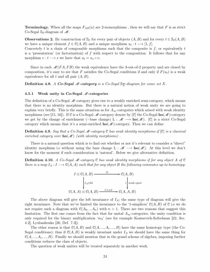
Definition 4.10. A Co-Segal M -category C has weak identity morphisms if for any object A of Cthere is a map IA : I −→ C(A,A) such that for any object B the following commutes up-to-homotopy:

I ⊗ C(A,B)

C(A,A)⊗ C(A,B) C(A,A,B)

C(A,B)

ϕAAB //

weak.equiv≀

��

∼= //

IA⊗Id

��

The above diagram will give the left invariance of IA; the same type of diagram will give theright invariance. Note that we’ve limited the invariance to the ‘1-simplices’ C(A,B) of C i.e we donot require such a diagram with C(A0, ...An) with n > 1. There are two reasons that suggest thislimitation. The first one comes from the fact that for unital A∞-categories, the unity condition isonly required for the binary multiplication ‘m2’ (see for example Kontsevich-Soibelman [22, Sec.4.2], Lyubashenko [30, Def. 7.3]).

The other reason is that C(A,B) and C(A, ..., Ai, ..., B) have the same homotopy type (the Co-Segal conditions); thus if C(A,B) is weakly invariant under IA we should have the same thing forC(A, ..., Ai, ..., B). Finally we should mention that in the grand scheme of algebra, imposing furtherconditions reduces the class of objects.

The question of weak unities will be treated separately in another work.

24

4.5.2 The classical examples

In the following discussion we will use the following conventions.

− By semi-enriched category we mean a structure given by the same data and axioms of anenriched category without the identities . We will say as well M -semi-category to mentionthe base M which contains the ‘Hom’. This is the generalized version of semi-monoids.

− As for M -categories, we have the morphism between M -semi-categories by simply ignoringthe data involving the identities.

− Our M -categories and M -semi-categories will always have a small set of objects.

The following proposition is the generalized version of Proposition 4.4.

Proposition 4.11. We have an equivalence between the following data:

1. an M -semi-category

2. a strict Co-Segal SX-diagram of M .

The proof is very similar and is straightforward. We give hereafter an outline for the case whereM is a monoidal category.

Sketch of proof. Let A be an M -semi-category with X = Ob(A ). We define the correspondingstrict Co-Segal SX-diagram F = (F,ϕ) as follows:

∗ each component FAB : SX(A,B) −→M is a constant functor :

{FAB([n, s]) = FAB([1, (A,B)]) := A (A,B) for all [n, s]

FAB(f) := IdA (A,B) for all f : [n, s] −→ [n′, s′] in SX(A,B)

∗ the laxity maps are given by the composition:

ϕs,t := cABC : A (B,C)⊗A (A,B) −→ A (A,C)

Conversely let F : (SX)2-op −→M be a strict Co-Segal SX-diagram. We simply show how we get

the composition of the M -semi-category which is denoted by MXF .

∗ First we have Ob(MXF ) = X.

∗ We take MXF (A,B) := FAB([1, (A,B)], for every A,B ∈ X.

∗ The laxity map ϕs,t for s = [1, (A,B)], t = [1, (B,C)] is a map of M

ϕs,t : MXF (B,C)⊗M

XF (A,B) −→M

XF (A,B,C)

where MXF (A,B,C) := FAC([2, (A,B,C)]).

25

∗ Now in SX(A,C) we have a unique map [2, (A,B,C)]σ10−→ [1, (A,C)] parametrized by the map

σ10 : 2 −→ 1 of Υ. The image of this map by FAC is a map

F (σ10) : MXF (A,C) −→M

XF (A,B,C)

which is invertible by hypothesis.

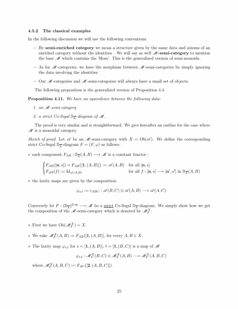
∗ And we take the composition cABC = F (σ10)−1 ◦ ϕs,t as illustrated in the the diagram below:

MXF (B,C)⊗MX

F (A,B) MXF (A,B,C)

MXF (A,C)

ϕs,t //

∼=F (σ10)

��

cABC

55❧❧❧❧❧❧❧❧❧

�

Remark 4.4. The previous equivalence will turn to be an equivalence of categories when we willhave the morphisms of S-diagrams.

4.6 Morphism of S-Diagrams

As our S-diagrams are lax morphisms of semi-bicategories, one can guess that a morphism of S-diagrams will be a transformations of lax morphisms in the sense of Bénabou. This is the sameapproach as in [3] where the morphism of path-objects were defined as transformations of colaxmorphisms.

But just like in [3] not every transformation will give a morphism of semi-enriched categories.In [3], a general transformation is called ‘M -premorphism’ and an M -morphism was defined asspecial M -premorphism.

Warning. In the following, we will only consider the transformations which will give the classicalnotion of morphism between semi-enriched categories. We decide not to mention ‘M -premorphisms’between S-diagrams.

We recall hereafter the definition of the transformations of morphisms of semi-bicategories weare going to work with. The following definition is slightly different from the standard one, eventhough in the monoidal case, it is the standard one.

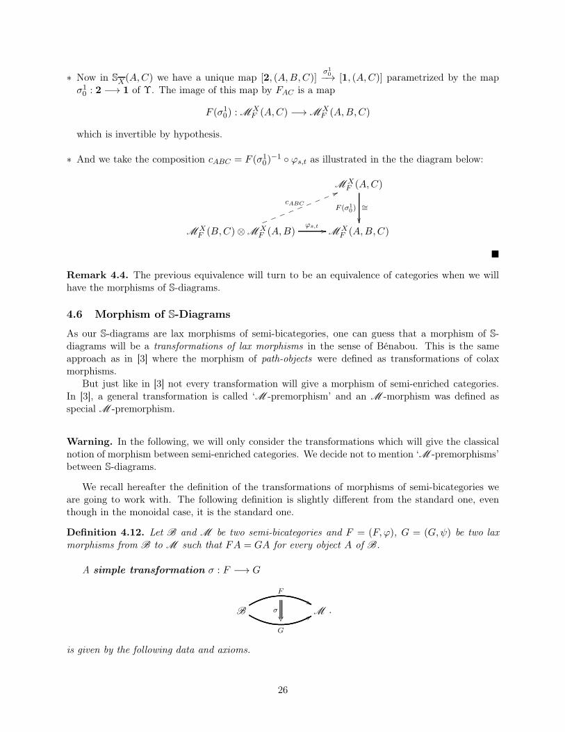
Definition 4.12. Let B and M be two semi-bicategories and F = (F,ϕ), G = (G,ψ) be two laxmorphisms from B to M such that FA = GA for every object A of B.

A simple transformation σ : F −→ G

B M

G

88

F

&&σ��

.

is given by the following data and axioms.

26

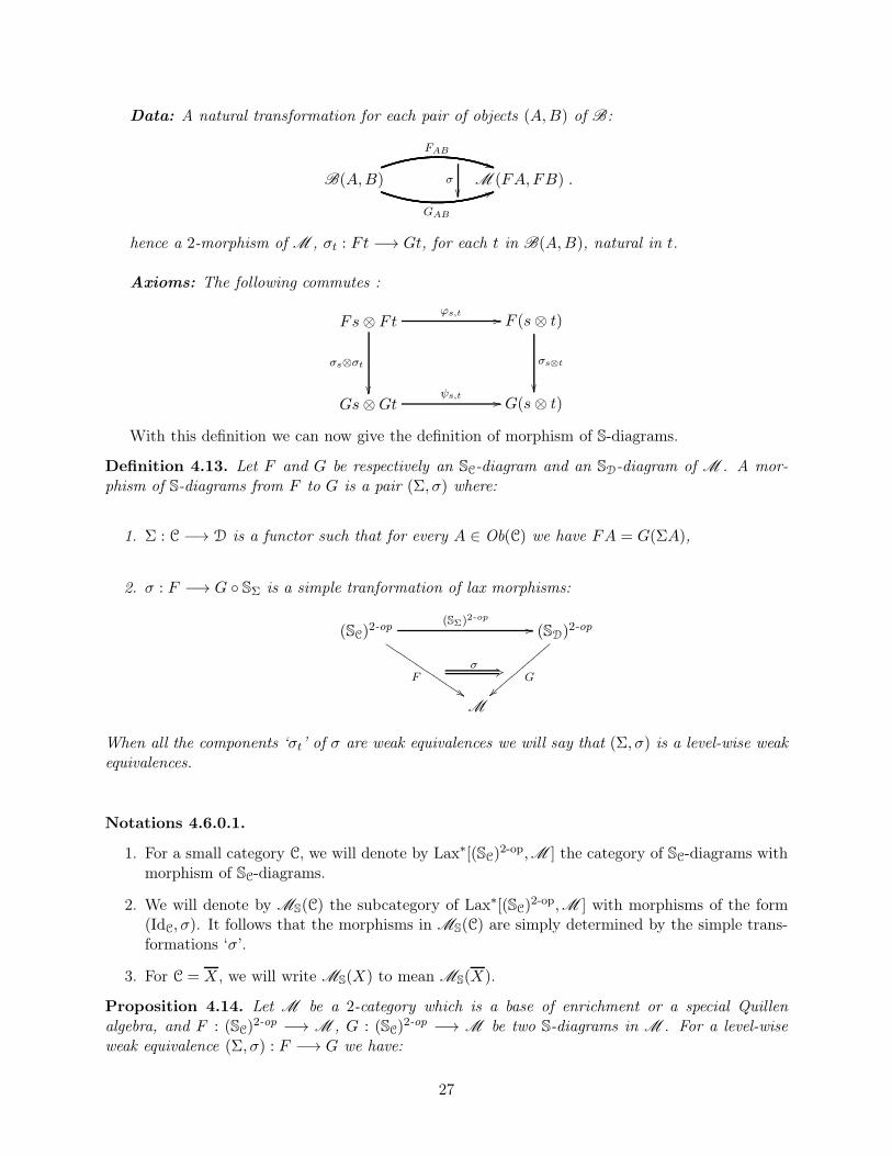
Data: A natural transformation for each pair of objects (A,B) of B:

B(A,B) M (FA,FB)

GAB

55

FAB

))σ��

.

hence a 2-morphism of M , σt : Ft −→ Gt, for each t in B(A,B), natural in t.

Axioms: The following commutes :

Fs⊗ Ft F (s⊗ t)

Gs⊗Gt G(s⊗ t)

ϕs,t //

σs⊗σt

��

σs⊗t

��ψs,t //

With this definition we can now give the definition of morphism of S-diagrams.

Definition 4.13. Let F and G be respectively an SC-diagram and an SD-diagram of M . A mor-phism of S-diagrams from F to G is a pair (Σ, σ) where:

1. Σ : C −→ D is a functor such that for every A ∈ Ob(C) we have FA = G(ΣA),

2. σ : F −→ G ◦ SΣ is a simple tranformation of lax morphisms:

(SC)2-op (SD)

2-op

M

(SΣ)2-op //

F

$$❏❏❏

❏❏❏❏

❏❏❏❏

❏❏

G

}}③③③③③③③③③③③

σ +3

When all the components ‘σt’ of σ are weak equivalences we will say that (Σ, σ) is a level-wise weakequivalences.

Notations 4.6.0.1.

1. For a small category C, we will denote by Lax∗[(SC)2-op,M ] the category of SC-diagrams with

morphism of SC-diagrams.

2. We will denote by MS(C) the subcategory of Lax∗[(SC)2-op,M ] with morphisms of the form

(IdC, σ). It follows that the morphisms in MS(C) are simply determined by the simple trans-formations ‘σ’.

3. For C = X , we will write MS(X) to mean MS(X).

Proposition 4.14. Let M be a 2-category which is a base of enrichment or a special Quillenalgebra, and F : (SC)

2-op −→ M , G : (SC)2-op −→ M be two S-diagrams in M . For a level-wise

weak equivalence (Σ, σ) : F −→ G we have:

27

1. If G is a Co-Segal S-diagram then so is F ,

2. If F is a Co-Segal S-diagram and if Σ is surjective on objects and full then G is also a Co-SegalS-diagram.

Remark 4.5. In the category MS(C) the condition required in (2) is automatically fulfilled becausethe morphism in MS(C) are of the form (IdC, σ).

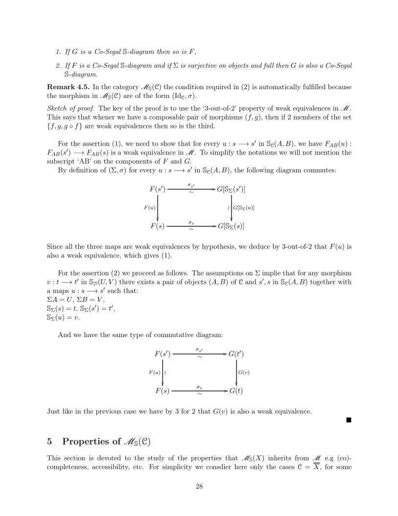
Sketch of proof. The key of the proof is to use the ‘3-out-of-2’ property of weak equivalences in M .This says that whener we have a composable pair of morphisms (f, g), then if 2 members of the set{f, g, g ◦ f} are weak equivalences then so is the third.

For the assertion (1), we need to show that for every u : s −→ s′ in SC(A,B), we have FAB(u) :FAB(s

′) −→ FAB(s) is a weak equivalence in M . To simplify the notations we will not mention thesubscript ‘AB’ on the components of F and G.

By definition of (Σ, σ) for every u : s −→ s′ in SC(A,B), the following diagram commutes:

F (s′) G[SΣ(s′)]

F (s) G[SΣ(s)]

σs′

∼//

F (u)

��

G[SΣ(u)]≀

��σs∼

//

Since all the three maps are weak equivalences by hypothesis, we deduce by 3-out-of-2 that F (u) isalso a weak equivalence, which gives (1).

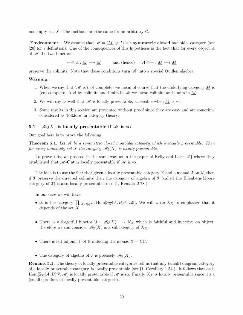
For the assertion (2) we proceed as follows. The assumptions on Σ implie that for any morphismv : t −→ t′ in SD(U, V ) there exists a pair of objects (A,B) of C and s′, s in SC(A,B) together witha maps u : s −→ s′ such that:ΣA = U , ΣB = V ,SΣ(s) = t, SΣ(s

′) = t′,SΣ(u) = v.

And we have the same type of commutative diagram:

F (s′) G(t′)

F (s) G(t)

σs′

∼//

F (u) ≀

��

G(v)

��σs∼

//

Just like in the previous case we have by 3 for 2 that G(v) is also a weak equivalence.�

5 Properties of MS(C)

This section is devoted to the study of the properties that MS(X) inherits from M e.g (co)-completeness, accessibility, etc. For simplicity we consdier here only the cases C = X , for some

28

nonempty set X. The methods are the same for an arbitrary C.

Environment: We assume that M = (M,⊗, I) is a symmetric closed monoidal category (see[20] for a definition). One of the consequences of this hypothesis is the fact that for every object Aof M the two functors

−⊗A :M −→M and (hence) A⊗− :M −→M

preserve the colimits. Note that these conditions turn M into a special Quillen algebra.

Warning.

1. When we say that ‘M is (co)-complete’ we mean of course that the underlying category M is(co)-complete. And by colimits and limits in M we mean colimits and limits in M .

2. We will say as well that M is locally presentable, accessible when M is so.

3. Some results in this section are presented without proof since they are easy and are sometimeconsidered as ‘folklore’ in category theory.

5.1 MS(X) is locally presentable if M is so

Our goal here is to prove the following

Theorem 5.1. Let M be a symmetric closed monoidal category which is locally presentable. Thenfor every nonempty set X the category MS(X) is locally presentable.

To prove this, we proceed in the same way as in the paper of Kelly and Lack [21] where theyestablished that M -Cat is locally presentable if M is so.

The idea is to use the fact that given a locally presentable category K and a monad T on K, thenif T preserve the directed colimits then the category of algebra of T (called the Eilenberg-Moorecategory of T) is also locally presentable (see [1, Remark 2.78]).

In our case we will have:

• K is the category∏

(A,B)∈X2 Hom[SX(A,B)op,M ]. We will write KX to emphasize that itdepends of the set X

• There is a forgetful functor U : MS(X) −→ KX which is faithful and injective on object,therefore we can consider MS(X) is a subcategory of KX .

• There is left adjoint Γ of U inducing the monad T = UΓ.

• The category of algebra of T is precisely MS(X).

Remark 5.1. The theory of locally presentable categories tell us that any (small) diagram categoryof a locally presentable category, is locally presentable (see [1, Corollary 1.54]). It follows that eachHom[SX(A,B)op,M ] is locally presentable if M is so. Finally KX is locally presentable since it’s a(small) product of locally presentable categories.

29

But before proving the Theorem 5.1 we must first show that MS(X) is co-complete to be ableto consider (filtered) colimits. This is given by the following

Theorem 5.2. Given a co-complete symmetric monoidal category M , for any nonempty set X thecategory MS(X) is co-complete.

Proof of Theorem 5.2. See Appendix C �

Proposition 5.3. The monad T = UΓ : KX −→ KX is finitary, that is, it preserves filtered colimits.

Proof of the proposition. Filtered and directed colimits are essentially the same and it’s known thata functor preserves filtered colimits if and only if it preserves directed colimits (see [1, Chap. 1,Thm 1.5 and Cor ]). This allows us to reduce the proof to directed colimits.

Recall that colimits in KX =∏

(A,B)∈X2 Hom[SX(A,B)op,M ] are computed factor-wise.

For F = (FAB) recall that TF = ([ΓF]AB) where Γ is the left adjoint of U (see AppendixB.1).3 To simplify the notation we will not mention the subscript ‘AB’. For each pair (A,B) theAB-component of ΓF is ΓF : SX(A,B)op −→M the functor given by:

• for t ∈ SX(A,B) we have

ΓF(t) =∐

(t0,··· ,tl)∈Dec(t)

F(t0)⊗ · · · ⊗ F(tl).

• for u : t −→ t′ , we have

ΓF(u) =∐

(u0,··· ,ul)∈Dec(u)

F(u0)⊗ · · · ⊗ F(ul)

where ui : ti −→ t′i.

Let λ < κ be an ordinal and (Fk)k∈λ be a λ-directed diagram in KX whose colimit is denotedby F∞.

For any l the diagonal functor d : λ −→∏i=0...l λ is cofinal therefore the following colimits are

the same

colim(k0,...,kl)∈λl+1{Fk0(t0)⊗ · · · ⊗ Fkl(tl)}

colimk∈λ{Fk(t0)⊗ · · · ⊗ Fk(tl)}

The first colimit is easy to compute as M is symmetric closed and we have

colim(k0,...,kl)∈λl+1{Fk0(t0)⊗ · · · ⊗ Fkntl} = F∞(t0)⊗ · · · ⊗ F∞

tl.

Consequently colimk∈λ{Fk(t0)⊗ · · · ⊗ Fktl} = F∞(t0)⊗ · · · ⊗ F∞(tl).

3Note that actually TF = ([UΓF]AB) but since U consists to forget the laxity maps it’s not necessary to mentionit.

30

From this we deduce successively that:

colimk∈λΓFk(t) = colimk∈λ{

∐

(t0,··· ,tl)∈Dec(t)

Fk(t0)⊗ · · · ⊗ Fk(tl)}

=∐

(t0,··· ,tl)∈Dec(t)

colimk∈λ{Fk(t0)⊗ · · · ⊗ Fk(tl)}

=∐

(t0,··· ,tl)∈Dec(t)

F∞(t0)⊗ · · · ⊗ F∞(tl)

= ΓF∞(t)

which shows that T = UΓ preserves directed colimits as desired. �

Now we can give the proof of Theorem 5.1 as follows.

Proof of Theorem 5.1. Thanks to Theorem C.9 we know that U : MS(X) −→ KX is monadictherefore MS(X) is equivalent to the category T-alg of T-algebra. Now since T is a finitary monadon the locally presentable category KX , we know from a classical result that T-alg (hence MS(X))is also locally presentable (see [1, Remark 2.78]). �

31

6 Locally Reedy 2-categories

In the following we give an ad hoc definition of a locally Reedy 2-category. One can generalize thisnotion to O-algebra but we will not go through that here. The horizontal composition in 2-categorieswill be denoted by ⊗.

Definition 6.1. A small 2-category C is called a locally Reedy 2-category if the following holds.

1. For each pair (A,B) of objects, the category C(A,B) is a classical Reedy 1-category;

2. The composition ⊗ : C(A,B)× C(B,C) −→ C(A,C) is a functor of Reedy categories i.e takesdirect (resp. inverse) morphisms to direct (resp. inverse) morphism.

Example 6.2. 1. The examples that motivated the above definition are of course the 2-categories,PD and SD, and their respective 1-opposite and 2-opposite 2-categories: (PD)

op, (SD)2-op,

etc. In particular (∆,+, 0) is a monoidal Reedy category (a locally Reedy 2-category with oneobject).

2. Any classical Reedy 1-category D can be considered as a 2-category with two objects 0 and1 with Hom(0, 1) = D, Hom(1, 0) = ∅; Hom(0, 0) = Hom(1, 1) = 1 (the unit category); thecomposition is the obvious one (left and right isomorphism of the cartesian product). It followthat any classical category is also a locally Reedy 2-category.

3. As any set is a (discrete) Reedy category, it follows that any 1-category viewed as a 2-categorywith only identity 2-morphisms is a locally Reedy 2-category. In that case the linear extensionare constant functor.

Warning. It’s important to notice that we’ve chosen to say ‘locally Reedy 2-category’ rather than‘Reedy 2-category’. The reason is that the later terminology may refer to the notion of ‘ReedyM-category’ (=enriched Reedy category) introduced by Angeltveit [2] when M = (Cat,×,1).

In our definition we’ve implicitly used the fact that if A and B are two classical Reedy categories,then there is a natural Reedy structure on the cartesian product A × B (see [17, Prop. 15.1.6]).This way we form a monoidal category of Reedy categories and morphisms of Reedy categories withthe cartesian product; the unit is the same i.e 1. We will denote by Cat×Reedy this monoidal category.

Our definition is equivalent to say that

Definition 6.3. A locally Reedy 2-category is a category enriched over Cat×Reedy.

Remark 6.1. 1. This definition can be generalized to locally Reedy n-categories, but we won’tconsider it, since the spirit of this paper is to use lower dimensional objects to define higherdimensional ones.

2. One can replace Cat×Reedy by a suitable monoidal category M -CatReedy⊗ of Reedy M -

categories in the sense of Angeltveit [2]; but we don’t know how relevant this would be.

3. We can also enrich over the category of generalized Reedy categories in the sense of Berger-Moerdijk [6] and in the sense of Cisinski [10, Chap. 8].

4. We can also push the definition far by considering not only Reedy O-algebras, but defining firsta Reedy multisorted operad as being multicategory enriched over Cat×Reedy,M -CatReedy

⊗, etc.

32

6.1 (Co)lax-latching and (Co)lax-matching objects

Let C be a locally Reedy 2-category (henceforth lr-category). Given a lax morphism or colaxmorphism F : C −→ M we would like to define the corresponding latching and matching objectsof F at a 1-morphism z of C. We will concentrate our discussion to the lax-latching object; leavingthe other cases to the reader. Our definitions are restricted to the case where C is equipped with aglobal linear extension which respects the composition. This means that we have an ordinal λsuch that the linear extension deg : C(A,B) −→ λ satisfies deg(g ⊗ f) = deg(g) + deg(f).

Note. We don’t know many examples other than the 2-categories that motivated this consideration,but we choose to have a common language for both PX , SX and the others 2-categories we can con-struct out of them. However it’s clear to see that for a classical Reedy 1-category D, if we view D asan lr-category with two objects (see Example 6.2) and if we declare both deg(Id0) = deg(Id1) = 0then D has this property.

We will consider lax morphism F : C −→ M which are unitary in the sense of Bénabou i.esuch that F(Id) = Id and the laxity maps F Id⊗Ff −→ F(Id⊗f) are the natural left and rightisomorphisms.

Let λ be an infinite ordinal containing ω. We can make λ into a monoidal category with theaddition; and we can consider it a usual as a 2-category with one object having as hom-category λ.

Definition 6.4. A locally Reedy 2-category C is simple if there exist an infinite ordinal λ such thatthe linear extension form a strict 2-functor deg : C −→ λ. Here on object deg : Ob(C) −→ {∗}

From this definition we have the following consequences:

− First if C is a simple lr-category then the composition reflects the identies; thus C is anir-O-algebra for the operad of 2-categories.

− For any object A ∈ C, we have deg(IdA) = 0 since deg(IdA) = deg(IdA⊗ IdA) = deg(IdA)+deg(IdA).

− Another important consequence is that a 1-morphism z, cannot appear in the set

⊗−1(z) =∐

l>1

{(s1, ..., sl);⊗(s1, ..., sl) = z}

if deg(si) > 0 for all i.

Using the Grothendieck construction For each pair (A,B) we have a composition diagramwhich is organized into a functor c : ∆epi −→ Cat and represented as:

C(A,B)∐

C(A,A1)× C(A1, B)∐

C(A,A1)× C(A1, A2)× C(A2, B) · · ·oo oooo

More precisely one defines:

− c(1) = C(A,B),

− c(n) =∐

(A,...,B) C(A,A1)× C(A,A1)× · · · × C(An−1, B).

33

Note that the morphisms in ∆epi are generated by the maps σni : n + 1 −→ n which are char-acterized by σni (i) = σni (i + 1) for i ∈ n = {0, · · · , n − 1} (see [31, p.177]). Then the functorc(σni ) : c(n + 1) −→ c(n) is the functor which consists to compose at the vertex Ai+1.

Let∫c be the category we obtained by the Grothendieck construction:

− the objects are pairs (n, a) with a ∈ Ob(c(n)). Such object (n, a) can be identified with ann-tuple of 1-morphisms (s1, ..., sn) with si ∈ C(Ai−1, Ai).

− a morphism γ : (n, a) −→ (m, b) is a pair γ = (f, u) where f : n −→ m is a morphism of ∆epi

and u : c(f)a −→ b is a morphism in c(m). Here c(f) : c(n) −→ c(m) is a functor (image off by c).

− the composite of γ = (f, u) and γ′ = (g, v) is γ′ ◦ γ := (g ◦ f, v ◦ c(g)u).

One can easily check that these data define a category. Note that for each n ∈ ∆epi the subcategoryof objects over n is isomorphic to c(n).

Claim. For a simple lr-category C and for each pair (A,B) there is a natural Reedy structure on∫c.

In fact one has a linear extension by setting deg(n, a) = deg(a) = deg(s1) + · · ·+ deg(sn) fora = (s1, ..., sn). A morphism γ = (f, u) : (n, a) −→ (m, b) is said to be a direct (resp. inverse) ifu is a direct (resp. inverse) morphism in c(m). The factorization axiom follows from the fact thatc(m) is a Reedy category.

Remark 6.2.

1. There is a general statement for the category∫F associated to any functor

F : D −→ Cat×Reedy.

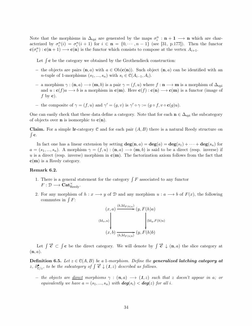
2. For any morphism of h : x −→ y of D and any morphism u : a −→ b of F (x), the followingcommutes in

∫F :

(x, a) (y, F (h)a)

(x, b) (y, F (h)b)

(h,IdF (h)a) //

(Idx,u)

��

(Idy,F (h)u)

��

(h,IdF (h)b)//

Let∫ −→

c ⊂∫c be the direct category. We will denote by

∫ −→c ↓ (n, a) the slice category at

(n, a).

Definition 6.5. Let z ∈ C(A,B) be a 1-morphism. Define the generalized latching category at

z, ∂•C/z, to be the subcategory of

∫ −→c ↓ (1, z) described as follows.

− the objects are direct morphisms γ : (n, a) −→ (1, z) such that z doesn’t appear in a; orequivalently we have a = (s1, ..., sn) with deg(si) < deg(z) for all i.

34

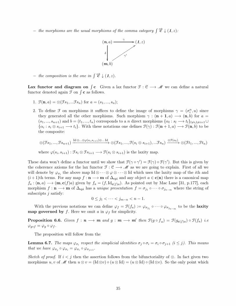
− the morphisms are the usual morphisms of the comma category∫ −→c ↓ (1, z):

(n, a) (1, z)

(m, b)

γ //

δ

��γ′

::ttttttttttttttt

− the composition is the one in∫ −→

c ↓ (1, z).

Lax functor and diagram on∫c Given a lax functor F : C −→ M we can define a natural

functor denoted again F on∫c as follows.

1. F(n, a) = ⊗(Fs1, ...Fsn) for a = (s1, ..., sn);

2. To define F on morphisms it suffices to define the image of morphisms γ = (σni , u) sincethey generated all the other morphisms. Such morphism γ : (n + 1, a) −→ (n, b) for a =(s1, ..., sn+1) and b = (t1, ..., tn) corresponds to a n direct morphisms {αl : sl −→ tl}l 6=i,l 6=i+1∪{αi : si ⊗ si+1 −→ ti}. With these notations one defines F(γ) : F(n + 1, a) −→ F(n, b) to bethe composite:

⊗(Fs1, ...,Fsn+1)Id⊗...⊗ϕ(si,si+1)⊗... Id−−−−−−−−−−−−−−−→ ⊗(Fs1, ...,F(si ⊗ si+1), ...Fsn)

⊗F(αl)−−−−→ ⊗(Ft1, ...,Ftn)

where ϕ(si, si+1) : Fsi ⊗ Fsi+1 −→ F(si ⊗ si+1) is the laxity map.

These data won’t define a functor until we show that F(γ ◦ γ′) = F(γ) ◦ F(γ′). But this is given bythe coherence axioms for the lax functor F : C −→ M as we are going to explain. First of all wewill denote by ϕσi the above map Id⊗ · · · ⊗ ϕ⊗ · · · ⊗ Id which uses the laxity map of the ith and(i+1)th terms. For any map f : n −→m of ∆epi and any object a ∈ c(n) there is a canonical mapfa : (n, a) −→ (m, c(f)a) given by fa = (f, Idc(f)a). As pointed out by Mac Lane [31, p.177], eachmorphism f : n −→ m of ∆epi has a unique presentation f = σj1 ◦ · · · ◦ σjn−m where the string ofsubscripts j satisfy:

0 ≤ j1 < · · · < jm−n < n− 1.

With the previous notations we can define ϕf = F(fa) := ϕσj1 ◦ · · · ◦ ϕσjn−mto be the laxity

map governed by f . Here we omit a in ϕf for simplicity.

Proposition 6.6. Given f : n −→ m and g : m −→ m′ then F(g ◦ fa) = F(gc(f)a) ◦ F(fa) i.eϕg◦f = ϕg ◦ ϕf .

The proposition will follow from the

Lemma 6.7. The maps ϕσi respect the simplicial identities σj ◦σi = σi ◦σj+1 (i ≤ j). This meansthat we have ϕσj ◦ ϕσi = ϕσi ◦ ϕσj+1 .

Sketch of proof. If i < j then the assertion follows from the bifunctoriality of ⊗. In fact given twomorphisms u, v of M then u⊗ v = (Id⊗v) ◦ (u⊗ Id) = (u⊗ Id) ◦ (Id⊗v). So the only point which

35

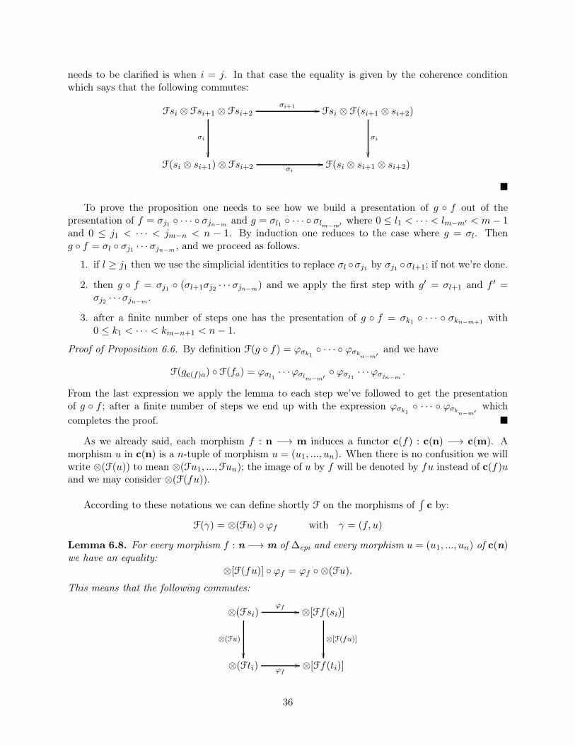
needs to be clarified is when i = j. In that case the equality is given by the coherence conditionwhich says that the following commutes:

Fsi ⊗ Fsi+1 ⊗ Fsi+2 Fsi ⊗ F(si+1 ⊗ si+2)

F(si ⊗ si+1)⊗ Fsi+2 F(si ⊗ si+1 ⊗ si+2)

σi+1 //

σi

��

σi

��

σi//

�

To prove the proposition one needs to see how we build a presentation of g ◦ f out of thepresentation of f = σj1 ◦ · · · ◦ σjn−m and g = σl1 ◦ · · · ◦ σlm−m′ where 0 ≤ l1 < · · · < lm−m′ < m− 1and 0 ≤ j1 < · · · < jm−n < n − 1. By induction one reduces to the case where g = σl. Theng ◦ f = σl ◦ σj1 · · · σjn−m , and we proceed as follows.

1. if l ≥ j1 then we use the simplicial identities to replace σl ◦σj1 by σj1 ◦σl+1; if not we’re done.

2. then g ◦ f = σj1 ◦ (σl+1σj2 · · · σjn−m) and we apply the first step with g′ = σl+1 and f ′ =σj2 · · · σjn−m .

3. after a finite number of steps one has the presentation of g ◦ f = σk1 ◦ · · · ◦ σkn−m+1 with0 ≤ k1 < · · · < km−n+1 < n− 1.

Proof of Proposition 6.6. By definition F(g ◦ f) = ϕσk1 ◦ · · · ◦ ϕσkn−m′and we have

F(gc(f)a) ◦ F(fa) = ϕσl1 · · ·ϕσlm−m′◦ ϕσj1 · · ·ϕσjn−m

.

From the last expression we apply the lemma to each step we’ve followed to get the presentationof g ◦ f ; after a finite number of steps we end up with the expression ϕσk1 ◦ · · · ◦ ϕσkn−m′

which

completes the proof. �

As we already said, each morphism f : n −→ m induces a functor c(f) : c(n) −→ c(m). Amorphism u in c(n) is a n-tuple of morphism u = (u1, ..., un). When there is no confusition we willwrite ⊗(F(u)) to mean ⊗(Fu1, ...,Fun); the image of u by f will be denoted by fu instead of c(f)uand we may consider ⊗(F(fu)).

According to these notations we can define shortly F on the morphisms of∫c by:

F(γ) = ⊗(Fu) ◦ ϕf with γ = (f, u)

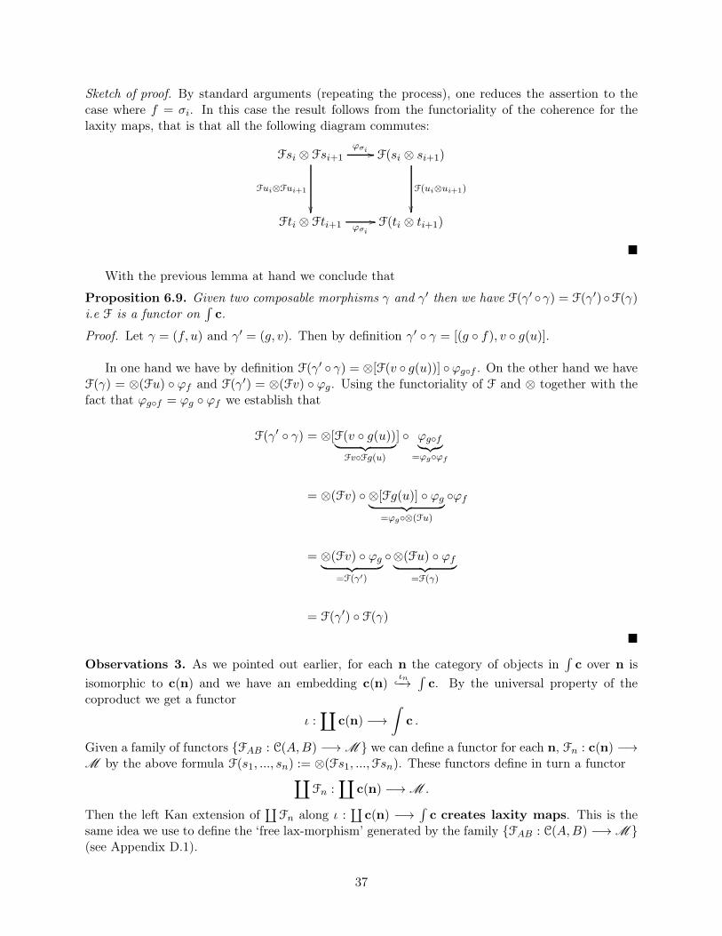
Lemma 6.8. For every morphism f : n −→ m of ∆epi and every morphism u = (u1, ..., un) of c(n)we have an equality:

⊗[F(fu)] ◦ ϕf = ϕf ◦ ⊗(Fu).

This means that the following commutes:

⊗(Fsi) ⊗[Ff(si)]

⊗(Fti) ⊗[Ff(ti)]

ϕf //

⊗(Fu)

��

⊗[F(fu)]

��

ϕf

//

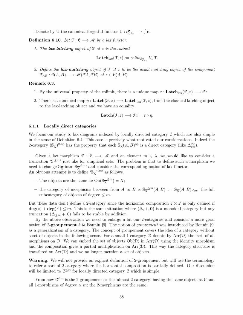
36

Sketch of proof. By standard arguments (repeating the process), one reduces the assertion to thecase where f = σi. In this case the result follows from the functoriality of the coherence for thelaxity maps, that is that all the following diagram commutes:

Fsi ⊗ Fsi+1 F(si ⊗ si+1)

Fti ⊗ Fti+1 F(ti ⊗ ti+1)

ϕσi //

Fui⊗Fui+1

��

F(ui⊗ui+1)

��

ϕσi

//

�

With the previous lemma at hand we conclude that

Proposition 6.9. Given two composable morphisms γ and γ′ then we have F(γ′ ◦γ) = F(γ′)◦F(γ)i.e F is a functor on

∫c.

Proof. Let γ = (f, u) and γ′ = (g, v). Then by definition γ′ ◦ γ = [(g ◦ f), v ◦ g(u)].

In one hand we have by definition F(γ′ ◦ γ) = ⊗[F(v ◦ g(u))] ◦ϕg◦f . On the other hand we haveF(γ) = ⊗(Fu) ◦ ϕf and F(γ′) = ⊗(Fv) ◦ ϕg. Using the functoriality of F and ⊗ together with thefact that ϕg◦f = ϕg ◦ ϕf we establish that

F(γ′ ◦ γ) = ⊗[F(v ◦ g(u))︸ ︷︷ ︸Fv◦Fg(u)

] ◦ ϕg◦f︸︷︷︸=ϕg◦ϕf

= ⊗(Fv) ◦ ⊗[Fg(u)] ◦ ϕg︸ ︷︷ ︸=ϕg◦⊗(Fu)

◦ϕf

= ⊗(Fv) ◦ ϕg︸ ︷︷ ︸=F(γ′)

◦⊗(Fu) ◦ ϕf︸ ︷︷ ︸=F(γ)

= F(γ′) ◦ F(γ)

�

Observations 3. As we pointed out earlier, for each n the category of objects in∫c over n is

isomorphic to c(n) and we have an embedding c(n)ιn−→

∫c. By the universal property of the

coproduct we get a functor

ι :∐

c(n) −→

∫c .

Given a family of functors {FAB : C(A,B) −→M } we can define a functor for each n, Fn : c(n) −→M by the above formula F(s1, ..., sn) := ⊗(Fs1, ...,Fsn). These functors define in turn a functor

∐Fn :

∐c(n) −→M .

Then the left Kan extension of∐

Fn along ι :∐

c(n) −→∫c creates laxity maps. This is the

same idea we use to define the ‘free lax-morphism’ generated by the family {FAB : C(A,B) −→M }(see Appendix D.1).

37

Denote by U the canonical forgetful functor U : ∂•C/z −→

∫c.

Definition 6.10. Let F : C −→M be a lax functor.

1. The lax-latching object of F at z is the colimit

Latchlax(F, z) := colim∂•C/z

U⋆ F.

2. Define the lax-matching object of F at z to be the usual matching object of the componentFAB : C(A,B) −→M (FA,FB) at z ∈ C(A,B).

Remark 6.3.

1. By the universal property of the colimit, there is a unique map ε : Latchlax(F, z) −→ Fz.

2. There is a canonical map η : Latch(F, z) −→ Latchlax(F, z), from the classical latching objectto the lax-latching object and we have an equality

Latch(F, z) −→ Fz = ε ◦ η.

6.1.1 Locally direct categories

We focus our study to lax diagrams indexed by locally directed category C which are also simplein the sense of Definition 6.4. This case is precisely what motivated our considerations. Indeed the2-category (SX)

2-op has the property that each SX(A,B)op is a direct category (like ∆opepi).

Given a lax morphism F : C −→ M and an element m ∈ λ, we would like to consider atruncation ‘F≤m’ just like for simplicial sets. The problem is that to define such a morphism weneed to change SX into ‘SX

≤m’ and consider the corresponding notion of lax functor.An obvious attempt is to define ‘SX

≤m’ as follows.

− The objects are the same i.e Ob(SX≤m) = X;

− the category of morphisms between from A to B is SX≤m(A,B) := SX(A,B)≤m, the full

subcategory of objects of degree ≤ m.

But these data don’t define a 2-category since the horizontal composition z ⊗ z′ is only defined ifdeg(z) + deg(z′) ≤ m. This is the same situation where (∆,+,0) is a monoidal category but anytruncation (∆≤n,+, 0) fails to be stable by addition.

By the above observation we need to enlarge a bit our 2-categories and consider a more geralnotion of 2-groupement à la Bonnin [9]. The notion of groupement was introduced by Bonnin [9]as a generalization of a category. The concept of groupement covers the idea of a category withouta set of objects in the following sense. For a small 1-category D denote by Arr(D) the ‘set’ of allmorphisms on D. We can embed the set of objects Ob(D) in Arr(D) using the identity morphismand the composition gives a partial multiplication on Arr(D). This way the category structure istransfered on Arr(D) and we no longer mention a set of objects.

Warning. We will not provide an explicit definition of 2-groupement but will use the terminologyto refer a sort of 2-category where the horizontal composition is partially defined. Our discussionwill be limited to C≤m for locally directed category C which is simple.

From now C≤m is the 2-groupement or the ‘almost 2-category’ having the same objects as C andall 1-morphisms of degree ≤ m; the 2-morphisms are the same.

38

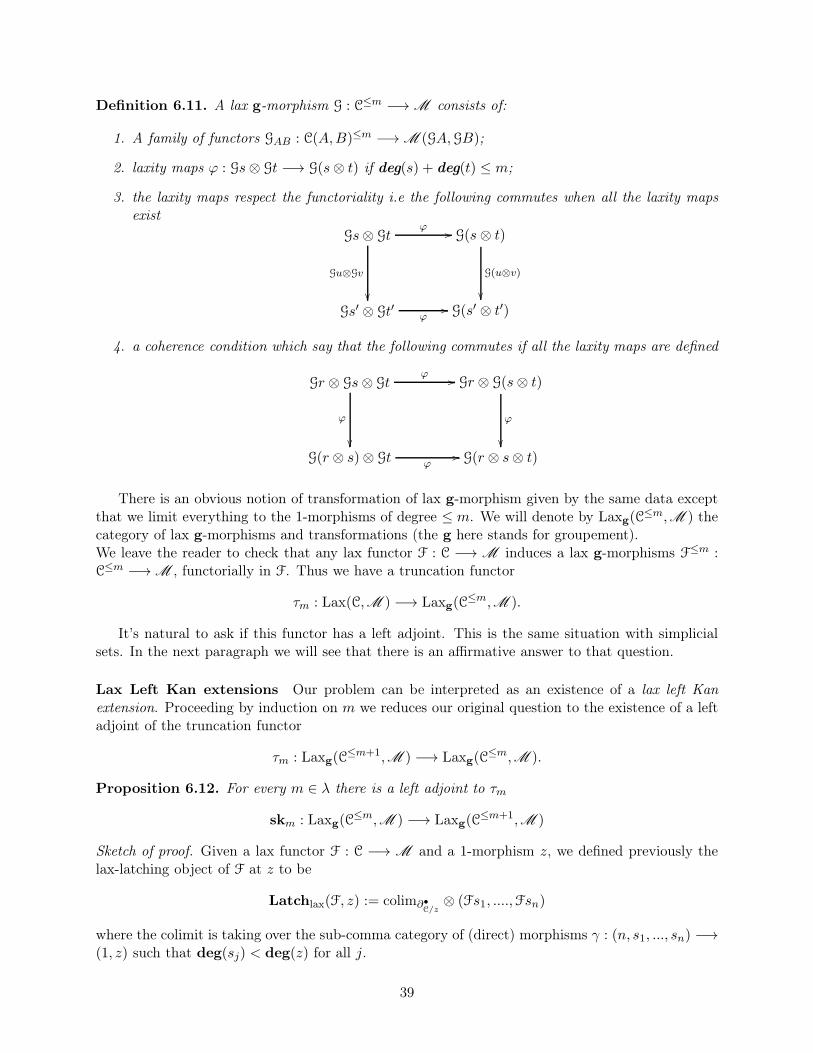
Definition 6.11. A lax g-morphism G : C≤m −→M consists of:

1. A family of functors GAB : C(A,B)≤m −→M (GA,GB);

2. laxity maps ϕ : Gs⊗ Gt −→ G(s⊗ t) if deg(s) + deg(t) ≤ m;

3. the laxity maps respect the functoriality i.e the following commutes when all the laxity mapsexist

Gs⊗ Gt G(s ⊗ t)

Gs′ ⊗ Gt′ G(s′ ⊗ t′)

ϕ //

Gu⊗Gv

��

G(u⊗v)

��

ϕ//

4. a coherence condition which say that the following commutes if all the laxity maps are defined

Gr ⊗ Gs⊗ Gt Gr ⊗ G(s⊗ t)

G(r ⊗ s)⊗ Gt G(r ⊗ s⊗ t)

ϕ //

ϕ

��

ϕ

��

ϕ//

There is an obvious notion of transformation of lax g-morphism given by the same data exceptthat we limit everything to the 1-morphisms of degree ≤ m. We will denote by Laxg(C

≤m,M ) thecategory of lax g-morphisms and transformations (the g here stands for groupement).We leave the reader to check that any lax functor F : C −→M induces a lax g-morphisms F≤m :C≤m −→M , functorially in F. Thus we have a truncation functor

τm : Lax(C,M ) −→ Laxg(C≤m,M ).

It’s natural to ask if this functor has a left adjoint. This is the same situation with simplicialsets. In the next paragraph we will see that there is an affirmative answer to that question.

Lax Left Kan extensions Our problem can be interpreted as an existence of a lax left Kanextension. Proceeding by induction on m we reduces our original question to the existence of a leftadjoint of the truncation functor

τm : Laxg(C≤m+1,M ) −→ Laxg(C

≤m,M ).

Proposition 6.12. For every m ∈ λ there is a left adjoint to τm

skm : Laxg(C≤m,M ) −→ Laxg(C

≤m+1,M )

Sketch of proof. Given a lax functor F : C −→ M and a 1-morphism z, we defined previously thelax-latching object of F at z to be

Latchlax(F, z) := colim∂•C/z⊗ (Fs1, ....,Fsn)

where the colimit is taking over the sub-comma category of (direct) morphisms γ : (n, s1, ..., sn) −→(1, z) such that deg(sj) < deg(z) for all j.

39

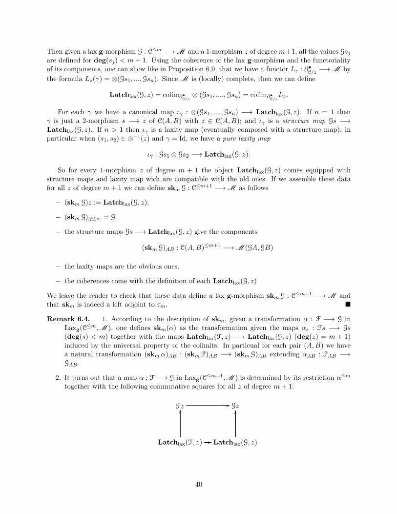
Then given a lax g-morphism G : C≤m −→M and a 1-morphism z of degree m+1, all the values Gsjare defined for deg(sj) < m+ 1. Using the coherence of the lax g-morphism and the functorialityof its components, one can show like in Proposition 6.9, that we have a functor Lz : ∂

•C/z −→M by

the formula Lz(γ) = ⊗(Gs1, ...,Gsn). Since M is (locally) complete, then we can define

Latchlax(G, z) = colim∂•C/z⊗ (Gs1, ....,Gsn) = colim∂•

C/zLz.

For each γ we have a canonical map ιγ : ⊗(Gs1, ....,Gsn) −→ Latchlax(G, z). If n = 1 thenγ is just a 2-morphism s −→ z of C(A,B) with z ∈ C(A,B); and ιγ is a structure map Gs −→Latchlax(G, z). If n > 1 then ιγ is a laxity map (eventually composed with a structure map); inparticular when (s1, s2) ∈ ⊗

−1(z) and γ = Id, we have a pure laxity map

ιγ : Gs1 ⊗ Gs2 −→ Latchlax(G, z).

So for every 1-morphism z of degree m + 1 the object Latchlax(G, z) comes equipped withstructure maps and laxity map wich are compatible with the old ones. If we assemble these datafor all z of degree m+ 1 we can define skm G : C≤m+1 −→M as follows

− (skm G)z := Latchlax(G, z);

− (skm G)|C≤m = G

− the structure maps Gs −→ Latchlax(G, z) give the components

(skm G)AB : C(A,B)≤m+1 −→M (GA,GB)

− the laxity maps are the obvious ones.

− the coherences come with the definition of each Latchlax(G, z)

We leave the reader to check that these data define a lax g-morphism skm G : C≤m+1 −→M andthat skm is indeed a left adjoint to τm. �

Remark 6.4. 1. According to the description of skm, given a transformation α : F −→ G inLaxg(C

≤m,M ), one defines skm(α) as the transformation given the maps αs : Fs −→ Gs(deg(s) < m) together with the maps Latchlax(F, z) −→ Latchlax(G, z) (deg(z) = m + 1)induced by the universal property of the colimits. In particual for each pair (A,B) we havea natural transformation (skm α)AB : (skm F)AB −→ (skm G)AB extending αAB : FAB −→GAB .

2. It turns out that a map α : F −→ G in Laxg(C≤m+1,M ) is determined by its restriction α≤m

together with the following commutative squares for all z of degree m+ 1:

Fz Gz

Latchlax(F, z) Latchlax(G, z)

//OO OO

//

40

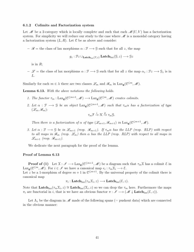
6.1.2 Colimits and Factorization system

Let M be a 2-category which is locally complete and such that each M (U, V ) has a factorizationsystem. For simplicity we will reduce our study to the case where M is a monoidal category havinga factorization system (L,R). Let C be as above and consider:

− R = the class of lax morphisms α : F −→ G such that for all z, the map

gz : Fz ∪Latchlax(F,z) Latchlax(G, z) −→ Gz

is in R;

− L = the class of lax morphisms α : F −→ G such that for all z the map αz : Fz −→ Gz is inL.

Similarly for each m ∈ λ there are two classes Lm and Rm in Laxg(C≤m,M ).

Lemma 6.13. With the above notations the following holds.

1. The functor τm : Laxg(C≤m+1,M ) −→ Laxg(C

≤m,M ) creates colimits.

2. Let α : F −→ G be an object Laxg(C≤m+1,M ) such that τmα has a factorization of type

(Lm,Rm):

τmFi−→ K

p−→ τmG.

Then there is a factorization of α of type (Lm+1,Rm+1) in Laxg(C≤m+1,M ).

3. Let α : F −→ G be in Lm+1 (resp. Rm+1). If τmα has the LLP (resp. RLP) with respectto all maps in Rm (resp. Lm) then α has the LLP (resp. RLP) with respect to all maps inLm+1 (resp. Rm+1).

We dedicate the next paragraph for the proof of the lemma.

Proof of Lemma 6.13

Proof of (1) Let X : I −→ Laxg(C≤m+1,M ) be a diagram such that τmX has a colimit E in

Laxg(C≤m,M ). For i ∈ I we have a canonical map ei : τmXi −→ E.

Let z be a 1-morphism of degree m+ 1 in C≤m+1. By the universal property of the colimit there iscanonical map

πi : Latchlax(τmXi, z) −→ Latchlax(E, z).

Note that Latchlax(τmXi, z) ∼= Latchlax(Xi, z) so we can drop the τm here. Furthermore the mapsπi are functorial in i, that is we have an obvious functor π : I −→ (M ↓ Latchlax(E, z)).

Let Λz be the diagram in M made of the following spans (= pushout data) which are connectedin the obvious manner:

41

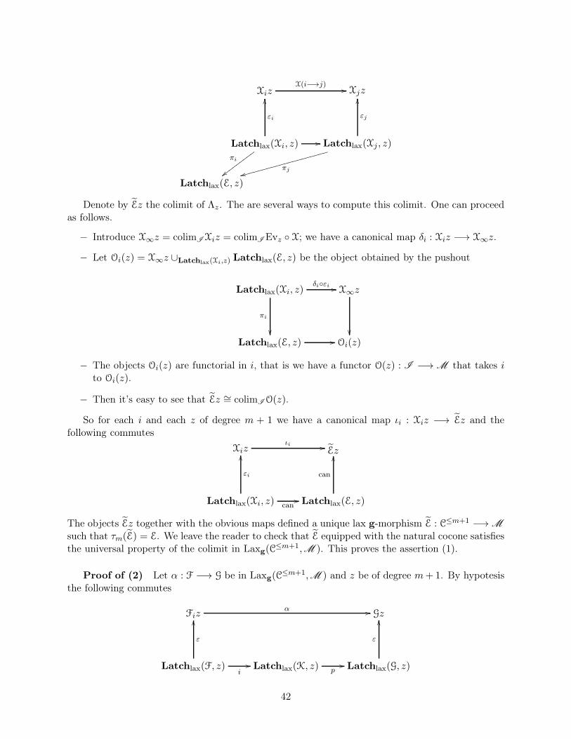
Xiz Xjz

Latchlax(Xi, z) Latchlax(Xj , z)

X(i−→j) //

εi

OO

εj

OO

//

Latchlax(E, z)

πi

{{✇✇✇✇✇✇✇✇✇

πjss❤❤❤❤❤❤❤❤❤

❤❤❤❤❤❤❤❤

❤❤❤

Denote by Ez the colimit of Λz. The are several ways to compute this colimit. One can proceedas follows.

− Introduce X∞z = colimIXiz = colimI Evz ◦ X; we have a canonical map δi : Xiz −→ X∞z.

− Let Oi(z) = X∞z ∪Latchlax(Xi,z) Latchlax(E, z) be the object obtained by the pushout

Latchlax(Xi, z) X∞z

Latchlax(E, z) Oi(z)

δi◦εi //

πi

�� ��//

− The objects Oi(z) are functorial in i, that is we have a functor O(z) : I −→M that takes ito Oi(z).

− Then it’s easy to see that Ez ∼= colimIO(z).

So for each i and each z of degree m + 1 we have a canonical map ιi : Xiz −→ Ez and thefollowing commutes

Xiz Ez

Latchlax(Xi, z) Latchlax(E, z)

ιi //

εi

OO

can

OO

can//

The objects Ez together with the obvious maps defined a unique lax g-morphism E : C≤m+1 −→M

such that τm(E) = E. We leave the reader to check that E equipped with the natural cocone satisfiesthe universal property of the colimit in Laxg(C

≤m+1,M ). This proves the assertion (1).

Proof of (2) Let α : F −→ G be in Laxg(C≤m+1,M ) and z be of degree m+1. By hypotesis

the following commutes

Fiz Gz

Latchlax(F, z) Latchlax(G, z)Latchlax(K, z)

α //

ε

OO

ε

OO

i//

p//

42

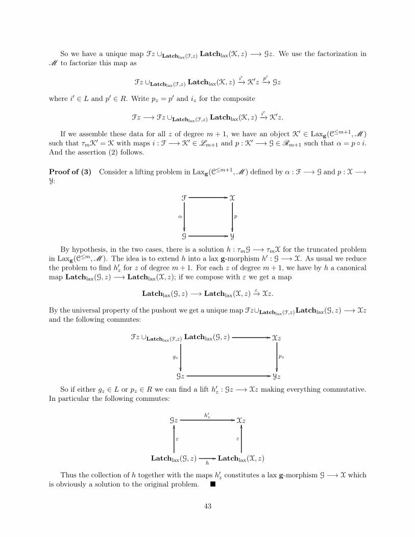
So we have a unique map Fz ∪Latchlax(F,z) Latchlax(K, z) −→ Gz. We use the factorization inM to factorize this map as

Fz ∪Latchlax(F,z) Latchlax(K, z)i′−→ K′z

p′−→ Gz

where i′ ∈ L and p′ ∈ R. Write pz = p′ and iz for the composite

Fz −→ Fz ∪Latchlax(F,z) Latchlax(K, z)i′−→ K′z.

If we assemble these data for all z of degree m + 1, we have an object K′ ∈ Laxg(C≤m+1,M )

such that τmK′ = K with maps i : F −→ K′ ∈ Lm+1 and p : K′ −→ G ∈ Rm+1 such that α = p ◦ i.

And the assertion (2) follows.

Proof of (3) Consider a lifting problem in Laxg(C≤m+1,M ) defined by α : F −→ G and p : X −→

Y:

F X

G Y

//

α

��

p

��//

By hypothesis, in the two cases, there is a solution h : τmG −→ τmX for the truncated problemin Laxg(C

≤m,M ). The idea is to extend h into a lax g-morphism h′ : G −→ X. As usual we reducethe problem to find h′z for z of degree m+1. For each z of degree m+ 1, we have by h a canonicalmap Latchlax(G, z) −→ Latchlax(X, z); if we compose with ε we get a map

Latchlax(G, z) −→ Latchlax(X, z)ε−→ Xz.

By the universal property of the pushout we get a unique map Fz∪Latchlax(F,z)Latchlax(G, z) −→ Xzand the following commutes:

Fz ∪Latchlax(F,z) Latchlax(G, z) Xz

Gz Yz

//

gz

��

pz

��//

So if either gz ∈ L or pz ∈ R we can find a lift h′z : Gz −→ Xz making everything commutative.In particular the following commutes:

Gz Xz

Latchlax(G, z) Latchlax(X, z)

h′z //

ε

OO

ε

OO

h//

Thus the collection of h together with the maps h′z constitutes a lax g-morphism G −→ X whichis obviously a solution to the original problem. �

43

6.2 Application: a model structure

We apply the previous material to establish the following

Theorem 6.14. Let M be a 2-category which is a locally model category and C be a locally Reedycategory which is simple and such that the degree deg : C −→ λ has a minimal value m0.

Then there is a model structure on the category Lax(C,M )u of all unitary lax morphisms; wherea morphism α : F −→ G is:

1. a weak equivalence if for all 1-morphism z, αz : Fz −→ Gz is a weak equivalence.

2. a fibration if for all 1-morphism z, αz : Fz −→ Gz is a fibration.

3. a cofibration if for all z the canonical map

gz : Fz ∪Latchlax(F,z) Latchlax(G, z) −→ Gz

is a cofibration

Corollary 6.15. For a monoidal model category M , the category MS(X) has a model structure,called the projective model structure, with the above three classes of weak equivalences, fibration,cofibration.

Proof of Theorem 6.14. The proof is very similar to the one given by Hovey [18, Thm 5.1.3] forclassical directed diagrams.An easy exercise shows that the above three classes of maps are closed under retracts. FollowingHovey, we will say that α is a good trivial cofibration if for all z

gz : Fz ∪Latchlax(F,z) Latchlax(G, z) −→ Gz

is a trivial cofibration.

Let deg−1(m0) be the set of all 1-morphisms of degree m0. For F ∈ Lax(C,M )u, since m0 isminimal then for any 1-morphism z ∈ deg−1(m0), there is no laxity maps Fs1 ⊗ Fs2 −→ Fz otherthan the isomorphism:

F Id⊗Fz∼=−→ Fz (F Id = Id).

Consequently it’s not hard to see that the category Laxg(C≤m0 ,M )u is just a product of copies

of M , i.e we have an isomorphism:

Laxg(C≤m0 ,M )u

∼=−→

∏

deg−1(m0)

M .

The above functor is the product of the evaluation functor at each z ∈ deg−1(m0). From theprevious isomorphism we deduce that Laxg(C

≤m0 ,M )u is cocomplete, and by Lemma 6.13 weestablish (by induction) that:

− Lax(C,M )u is cocomplete; it’s also complete since lax morphisms behave nicely with limits.

− Any map α can be factorized as a cofibration followed by a trivial fibration.

− Any map α can be factorized as a good trivial cofibration followed by a fibration.

44

− Good trivial cofibrations have the LLP with respect to all fibrations; and trivial fibrationshave the RLP with respect to all cofibrations.

Finally following the same method as Hovey one shows using a retract argument that every mapwhich is both a weak equivalence and a cofibration is a good trivial cofibration. �

Remark 6.5. For a classical Reedy 1-category D, if we view it as an lr-category which is simple,then the previous theorem gives the same model structure for diagrams in M indexed by D (see[18, Thm 5.1.3]).

7 A model structure on MS(X)

In this section we want to show, with a different method that for a fixed set X, the category SX-diagrams whose objects are called pre-cosegal categories has a model structure when M is monoidalmodel category. In the first case we will assume that M is cofibrantly generated model categorywith a set I (resp. J) of generating cofibrations (resp. acyclic cofibrations).

The model structure will be obtained by transfer of the model structure on the categoryKX =

∏(A,B)∈X2 Hom[SX(A,B)op,M ] along the monadic adjunction MS(X)⇆ KX .

On KX we will consider for our purposes the projective and injective model structure. Each ofthese model stuctures is the product of the one on each factor KX,AB = Hom[SX(A,B)op,M ]. Sinceeach SX(A,B) is an inverse category (like ∆epi) the projective and Reedy model structure on thepresheaf category KX,AB are the same. In fact the identity is an isomorphism of model categoriesbetween (KX,AB)proj and (KX,AB)Reedy see [4, 3.17], [18, Ch. 5]. In the last reference one viewsKX,AB as a functor category where the source is the directed category SX(A,B)op.The reader can find in [4, Prop 3.3], [17, Ch. 11.6; Ch.15 ],[18, Ch. 5], [29, A.3.3] [35, Ch. 7.6.2], adescription of these model structures on diagram categories.

Denote by KX-proj (resp. KX-inj) the projective (resp. injective) model structure on KX .These are cofibrantly generated model categories as (small) product of such model categories.The generating cofibrations and acyclic cofibration are respectively I• =

∏(A,B)∈X2 IAB and J• =∏

(A,B)∈X2 JAB, where IAB (resp. JAB) is the corresponding set of cofibration (resp. acyclic cofi-brations) in Hom[SX(A,B)op,M ]. For KX-proj one can actually tell more about the sets IAB andJAB ; the reader can find a nice description in the above references.

In contrast to the projective model structure, there is not an explicit characterization in KX-inj

for the generating set of (trivial) cofibrations. The generating cofibrations are known so far to be(trivial) cofibrations between presentable objects see [4], [29], [35] and references therein.

Extra hypothesis on M For the moment we will assume that all objects of M are cofibrant

The following lemma due to Schwede-Shipley [34] is the key step for the transfer of the modelstructure on KX to MS(X) through the monadic adjunction

U : MS(X)⇄ KX : Γ

Lemma 7.1. Let T be a monad on a cofibrantly generated model category K, whose underlyingfunctor commutes with directed colimits. Let I be the set of generating cofibrations and J be the set

45

of generating acyclic cofibrations for K. Let IT and JT be the images of these sets under the freeT-algebra functor. Assume that the domains of IT and JT are small relative to IT-cell and JT-cellrespectively. Suppose that

1. every regular JT-cofibration is a weak equivalence, or

2. every object of K is fibrant and every T-algebra has a path object.

Then the category of T-algebras is a cofibranty generated model category with IT a generating setof cofibrations and JT a generating set of acyclic cofibrations.

In our case we will need only to show that the condition (1) holds. We do this in the nextparagraph.

Note. In the formulation of Schwede-Shipley [34], IT-cell and JT-cell are respectively denoted byIT-cofreg and JT-cofreg.

7.1 Pushouts in MS(X)

Our goal here is to understand the pushout in MS(X) of Γα where α : A −→ B is a (trivial)cofibration in KX-inj or KX-proj.

By construction Γ preserves level-wise cofibrations and weak equivalences in KX so Γα is clearlya level-wise (trivial) cofibration if α is a (trivial) cofibration.

For an object F of MS(X) we want to analyse the pushout of ΓBΓα←− ΓA −→ F. Before going to

this task we start below with a constant case; we consider three objects with lax morphisms whichare coherent. The goal is to outline how one builds laxity maps when we move each of the threeobjects.

Analyze of the constant case Let m1,m2,m3,m12,m23 and m be objects of M with maps:

− ϕ : m1 ⊗m2 ⊗m3 −→ m,

− ϕ1,2 : m1 ⊗m2 −→ m12,

− ϕ2,3 : m2 ⊗m3 −→ m23,

− ϕ1,23 : m1 ⊗m23 −→ m,

− ϕ12,3 : m12 ⊗m3 −→ m,

Assume moreover that the following ‘associativity condition’ holds:

ϕ12,3 ◦ (ϕ1,2 ⊗ Idm3) = ϕ1,23 ◦ (Idm1 ⊗ϕ2,3) = ϕ.

These equalities are piece of the coherence conditions required for the laxity maps: think F (s) =m1, F (t) = m2, F (u) = m3, F (s ⊗ t) = m12, ϕt,s = ϕ1,2, etc. We’ve considered only three genericobjects because the coherences for lax morphisms involves three terms.

Terminology. We will say that the objects mi,mij together with the maps ϕ satisfying the previousequality form a 3-ary coherent system. There is also a notion of n-ary-coherent system whenwe consider n objects m1, ...,mn with compatible laxity maps. These are the ‘constant data’ of laxmorphism between O-algebras.

46

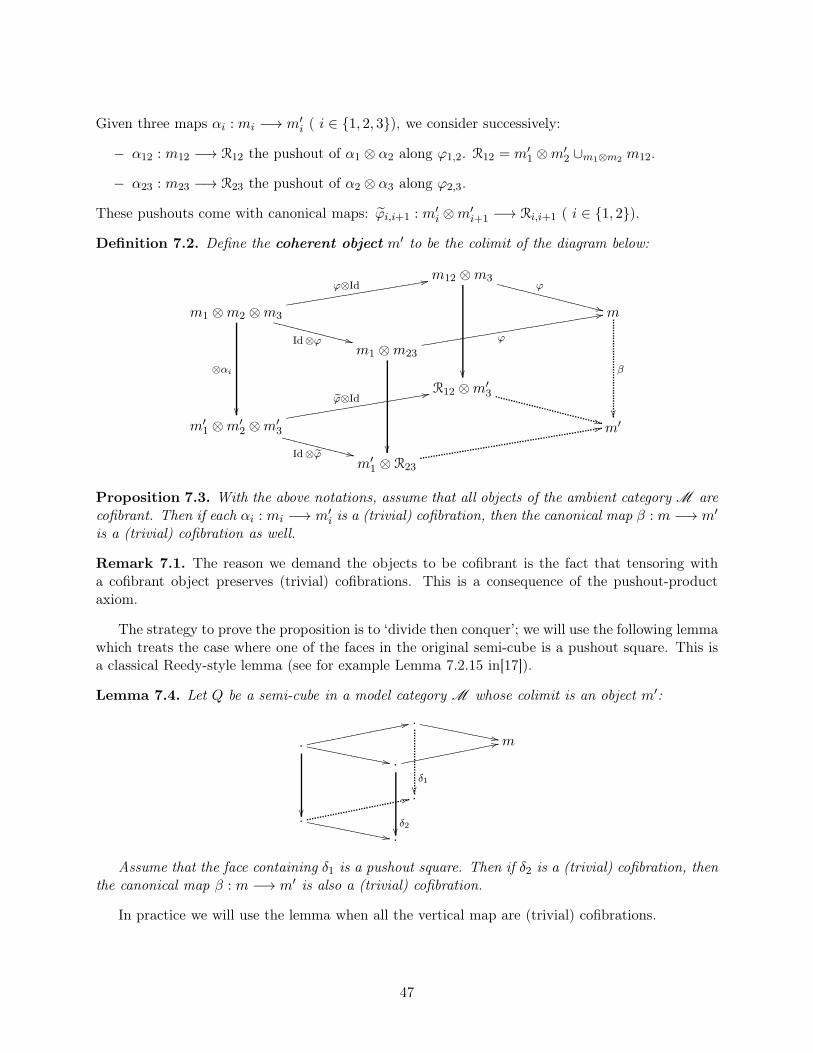
Given three maps αi : mi −→ m′i ( i ∈ {1, 2, 3}), we consider successively:

− α12 : m12 −→ R12 the pushout of α1 ⊗ α2 along ϕ1,2. R12 = m′1 ⊗m

′2 ∪m1⊗m2 m12.

− α23 : m23 −→ R23 the pushout of α2 ⊗ α3 along ϕ2,3.

These pushouts come with canonical maps: ϕi,i+1 : m′i ⊗m

′i+1 −→ Ri,i+1 ( i ∈ {1, 2}).

Definition 7.2. Define the coherent object m′ to be the colimit of the diagram below:

m1 ⊗m2 ⊗m3

m12 ⊗m3

m1 ⊗m23

m

ϕ⊗Id22❞❞❞❞❞❞❞❞❞❞❞❞❞❞❞❞❞❞❞❞❞❞

Id⊗ϕ ++❲❲❲❲❲❲❲❲

❲❲❲❲❲

ϕ

++❲❲❲❲❲❲❲❲

❲❲❲❲❲❲❲❲

❲

ϕ

22❞❞❞❞❞❞❞❞❞❞❞❞❞❞❞❞❞❞❞❞❞❞❞❞❞❞❞❞

m′1 ⊗m

′2 ⊗m

′3

R12 ⊗m′3

m′1 ⊗ R23

m′

ϕ⊗Id22❞❞❞❞❞❞❞❞❞❞❞❞❞❞❞❞❞❞❞❞❞❞

⊗αi

��++

��

�� β

��

Id⊗ϕ ++❲❲❲❲❲❲❲❲

❲❲❲❲22

Proposition 7.3. With the above notations, assume that all objects of the ambient category M arecofibrant. Then if each αi : mi −→ m′

i is a (trivial) cofibration, then the canonical map β : m −→ m′

is a (trivial) cofibration as well.

Remark 7.1. The reason we demand the objects to be cofibrant is the fact that tensoring witha cofibrant object preserves (trivial) cofibrations. This is a consequence of the pushout-productaxiom.

The strategy to prove the proposition is to ‘divide then conquer’; we will use the following lemmawhich treats the case where one of the faces in the original semi-cube is a pushout square. This isa classical Reedy-style lemma (see for example Lemma 7.2.15 in[17]).

Lemma 7.4. Let Q be a semi-cube in a model category M whose colimit is an object m′:

.

.

.

.

22❡❡❡❡❡❡❡❡❡❡❡❡❡❡❡❡

��

δ1��22

.

m

.

22❡❡❡❡❡❡❡❡❡❡❡❡❡❡❡

δ2��

,,❨❨❨❨❨❨❨❨❨❨

❨❨❨,,❨❨❨❨❨

❨❨❨❨❨❨❨

,,❨❨❨❨❨❨❨❨❨❨

❨❨❨

Assume that the face containing δ1 is a pushout square. Then if δ2 is a (trivial) cofibration, thenthe canonical map β : m −→ m′ is also a (trivial) cofibration.

In practice we will use the lemma when all the vertical map are (trivial) cofibrations.

47

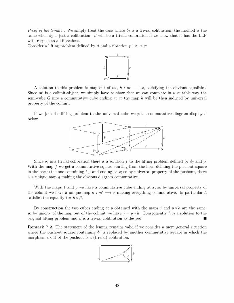
Proof of the lemma . We simply treat the case where δ2 is a trivial cofibration; the method is thesame when δ2 is just a cofibration. β will be a trivial cofibration if we show that it has the LLPwith respect to all fibrations.Consider a lifting problem defined by β and a fibration p : x։ y:

m x

m′ y

i //

β

��

p

����j //

A solution to this problem is map out of m′, h : m′ −→ x, satisfying the obvious equalities.Since m′ is a colimit-object, we simply have to show that we can complete in a suitable way thesemi-cube Q into a commutative cube ending at x; the map h will be then induced by universalproperty of the colimit.

If we join the lifting problem to the universal cube we get a commutative diagram displayedbelow

.

.

.

.

22❡❡❡❡❡❡❡❡❡❡❡❡❡❡❡❡

��

δ1��22❡❡❡❡❡❡❡❡❡❡❡❡❡❡❡❡

.

m

.m′

22❡❡❡❡❡❡❡❡❡❡❡❡❡❡❡� _

δ2 ≀��

β

��22

,,❨❨❨❨❨❨❨❨❨❨

❨❨❨,,❨❨❨❨❨

❨❨❨❨❨❨❨

,,❨❨❨❨❨❨❨❨❨❨

❨❨❨,,

x

y

i //

j //

p

����

f♠♠♠♠♠♠♠♠♠♠♠♠♠♠♠♠♠♠♠♠♠♠♠♠♠♠♠

66♠♠♠♠♠♠♠♠g

33

hsssssss

99ssssssssss

Since δ2 is a trivial cofibration there is a solution f to the lifting problem defined by δ2 and p.With the map f we get a commutative square starting from the horn defining the pushout squarein the back (the one containing δ1) and ending at x; so by universal property of the pushout, thereis a unique map g making the obvious diagram commutative.

With the maps f and g we have a commutative cube ending at x, so by universal property ofthe colimit we have a unique map h : m′ −→ x making everything commutative. In particular hsatisfies the equality i = h ◦ β.

By construction the two cubes ending at y obtained with the maps j and p ◦ h are the same,so by unicity of the map out of the colimit we have j = p ◦ h. Consequently h is a solution to theoriginal lifting problem and β is a trivial cofibration as desired. �

Remark 7.2. The statement of the lemma remains valid if we consider a more general situationwhere the pushout square containing δ1 is replaced by another commutative square in which themorphism ε out of the pushout is a (trivial) cofibration:

. .

. .

.

//

��

δ1

��

}}44

//

� q

ε##❋

❋❋❋❋

48

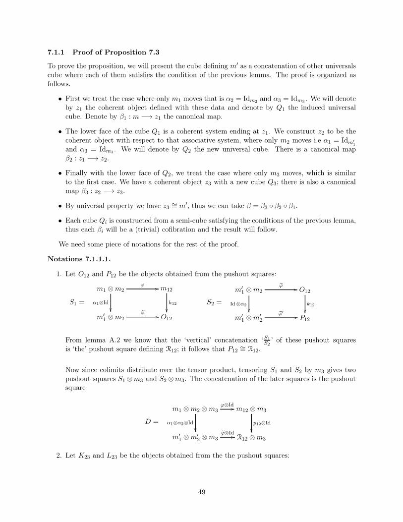
7.1.1 Proof of Proposition 7.3

To prove the proposition, we will present the cube defining m′ as a concatenation of other universalscube where each of them satisfies the condition of the previous lemma. The proof is organized asfollows.

• First we treat the case where only m1 moves that is α2 = Idm2 and α3 = Idm3 . We will denoteby z1 the coherent object defined with these data and denote by Q1 the induced universalcube. Denote by β1 : m −→ z1 the canonical map.

• The lower face of the cube Q1 is a coherent system ending at z1. We construct z2 to be thecoherent object with respect to that associative system, where only m2 moves i.e α1 = Idm′

1

and α3 = Idm3 . We will denote by Q2 the new universal cube. There is a canonical mapβ2 : z1 −→ z2.

• Finally with the lower face of Q2, we treat the case where only m3 moves, which is similarto the first case. We have a coherent object z3 with a new cube Q3; there is also a canonicalmap β3 : z2 −→ z3.

• By universal property we have z3 ∼= m′, thus we can take β = β3 ◦ β2 ◦ β1.

• Each cube Qi is constructed from a semi-cube satisfying the conditions of the previous lemma,thus each βi will be a (trivial) cofibration and the result will follow.

We need some piece of notations for the rest of the proof.

Notations 7.1.1.1.

1. Let O12 and P12 be the objects obtained from the pushout squares:

S1 =

m1 ⊗m2 m12

m′1 ⊗m2 O12

ϕ //

α1⊗Id

��h12

��ϕ //

S2 =

m′1 ⊗m2 O12

m′1 ⊗m

′2 P12

ϕ //

Id⊗α2

��k12

��ϕ′//

From lemma A.2 we know that the ‘vertical’ concatenation ‘S1S2

’ of these pushout squaresis ‘the’ pushout square defining R12; it follows that P12

∼= R12.

Now since colimits distribute over the tensor product, tensoring S1 and S2 by m3 gives twopushout squares S1⊗m3 and S2⊗m3. The concatenation of the later squares is the pushoutsquare

D =

m1 ⊗m2 ⊗m3 m12 ⊗m3

m′1 ⊗m

′2 ⊗m3 R12 ⊗m3

ϕ⊗Id //

α1⊗α2⊗Id

��p12⊗Id

��ϕ⊗Id //

2. Let K23 and L23 be the objects obtained from the the pushout squares:

49

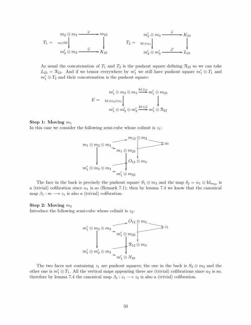
T1 =

m2 ⊗m3 m23

m′2 ⊗m3 K23

ϕ //

α2⊗Id

�� ��ϕ //

T2 =

m′2 ⊗m3 K23

m′2 ⊗m

′3 L23

ϕ //

Id⊗α3

�� ��ϕ′//

As usual the concatenation of T1 and T2 is the pushout square defining R23 so we can takeL23 = R23. And if we tensor everywhere by m′

1 we still have pushout square m′1 ⊗ T1 and

m′1 ⊗ T2 and their concatenation is the pushout square:

E =

m′1 ⊗m2 ⊗m3 m′

1 ⊗m23

m′1 ⊗m

′2 ⊗m

′3 m′

1 ⊗ R23

Id⊗ϕ//

Id⊗α2⊗α3

�� ��Id⊗ϕ //

Step 1: Moving m1

In this case we consider the following semi-cube whose colimit is z1:

m1 ⊗m2 ⊗m3

m12 ⊗m3

m′1 ⊗m2 ⊗m3

O12 ⊗m3

22❡❡❡❡❡❡❡❡

��

��22❡❡❡❡❡❡❡❡

m1 ⊗m23

m

m′1 ⊗m23

22❡❡❡❡❡❡❡❡❡❡❡❡❡❡

��

,,❨❨❨,,❨❨❨❨❨

❨❨❨

,,❨❨

The face in the back is precisely the pushout square S1 ⊗m3 and the map δ2 = α1 ⊗ Idm23 isa (trivial) cofibration since α1 is so (Remark 7.1); then by lemma 7.4 we know that the canonicalmap β1 : m −→ z1 is also a (trivial) cofibration.

Step 2: Moving m2

Introduce the following semi-cube whose colimit is z2:

m′1 ⊗m2 ⊗m3

O12 ⊗m3

m′1 ⊗m

′2 ⊗m3

R12 ⊗m3

22❡❡❡❡❡❡❡❡

��

��22❡❡❡❡❡❡❡❡

m′1 ⊗m23

z1

m′1 ⊗N23

22❡❡❡❡❡❡❡❡❡❡❡❡❡❡

��

,,❨❨,,❨❨❨❨❨

❨❨❨

,,❨❨

The two faces not containing z1 are pushout squares; the one in the back is S2 ⊗m3 and theother one is m′

1 ⊗ T1. All the vertical maps appearing there are (trivial) cofibrations since α2 is so,therefore by lemma 7.4 the canonical map β2 : z1 −→ z2 is also a (trivial) cofibration.

50

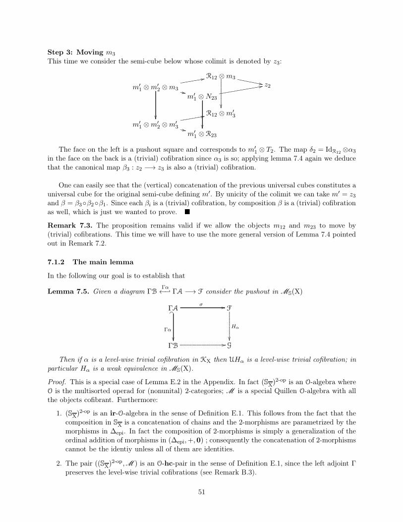
Step 3: Moving m3

This time we consider the semi-cube below whose colimit is denoted by z3:

m′1 ⊗m

′2 ⊗m3

R12 ⊗m3

m′1 ⊗m

′2 ⊗m

′3

R12 ⊗m′3

22❡❡❡❡❡❡❡❡

��

��22❡❡❡❡❡❡❡❡

m′1 ⊗N23

z2

m′1 ⊗R23

22❡❡❡❡❡❡❡❡❡❡❡❡❡❡

��

,,❨❨,,❨❨❨❨❨

❨❨❨

,,❨❨

The face on the left is a pushout square and corresponds to m′1 ⊗ T2. The map δ2 = IdR12 ⊗α3

in the face on the back is a (trivial) cofibration since α3 is so; applying lemma 7.4 again we deducethat the canonical map β3 : z2 −→ z3 is also a (trivial) cofibration.

One can easily see that the (vertical) concatenation of the previous universal cubes constitutes auniversal cube for the original semi-cube defining m′. By unicity of the colimit we can take m′ = z3and β = β3◦β2◦β1. Since each βi is a (trivial) cofibration, by composition β is a (trivial) cofibrationas well, which is just we wanted to prove. �

Remark 7.3. The proposition remains valid if we allow the objects m12 and m23 to move by(trivial) cofibrations. This time we will have to use the more general version of Lemma 7.4 pointedout in Remark 7.2.

7.1.2 The main lemma

In the following our goal is to establish that

Lemma 7.5. Given a diagram ΓBΓα←− ΓA −→ F consider the pushout in MS(X)

ΓA F

ΓB G

σ //_�

Γα

��

Hα

��//

Then if α is a level-wise trivial cofibration in KX then UHα is a level-wise trivial cofibration; inparticular Hα is a weak equivalence in MS(X).

Proof. This is a special case of Lemma E.2 in the Appendix. In fact (SX)2-op is an O-algebra where

O is the multisorted operad for (nonunital) 2-categories; M is a special Quillen O-algebra with allthe objects cofibrant. Furthermore:

1. (SX)2-op is an ir-O-algebra in the sense of Definition E.1. This follows from the fact that the

composition in SX is a concatenation of chains and the 2-morphisms are parametrized by themorphisms in ∆epi. In fact the composition of 2-morphisms is simply a generalization of theordinal addition of morphisms in (∆epi,+,0) ; consequently the concatenation of 2-morphismscannot be the identiy unless all of them are identities.

2. The pair ((SX)2-op,M ) is an O-hc-pair in the sense of Definition E.1, since the left adjoint Γ

preserves the level-wise trivial cofibrations (see Remark B.3).

51

We have MS(X) = LaxO-alg((SX)2-op,M ). �

Remark 7.4. It’s important to notice that in the lemma we’ve considered α a level-wise cofibrationin KX ; these are precisely the injective cofibrations therein. But this situation covers also theprojective case, since projective cofibrations are also injective ones.So in either KX-proj or KX-proj, the pushout of Γα is a lewel-wise weak equivalence and the condtion(1) of lemma 7.1 will hold.

7.2 The projective model structure

According to a well know result on diagram categories in cofibrantly generated model category,see [17, Theorem 11.6.1], each diagram category Hom[SX(A,B)op,M ] has a cofibrantly generatedmodel structure which is know to be the projective model structure.

In these settings a morphism σ : F −→ G is:

• A weak equivalence in Hom[SX(A,B)op,M ] if it is a level-wise equivalence: for every w thecomponent σw : Fw −→ Gw is a weak equivalence in M ,

• A fibration in Hom[SX(A,B)op,M ] if it is a level-wise fibration: σw : Fw −→ Gw is a (acyclic)fibration in M .

• A trivial fibration is a map which is both a fibration and a weak equivalence.

Left adjoint of evaluations For any object w ∈ SX(A,B)op the evalutation functor at w :Evw : Hom[SX(A,B)op,M ] −→M has a left adjoint

Fw− : M −→ Hom[SX(A,B)op,M ]

One defines Fw− by ‘the body’ of the Yoneda functor Yw (see [17, Section 11.5.21 ]):

Fwm = m⊗ Yw =∐

Hom(w,−)

m, for m ∈M .

This means that for v ∈ SX(A,B)op, Fwm(v) is the coproduct of copies of m indexed by the setHomSX(A,B)op(w, v). The fact that Fw− has the desired properties follows from the Yoneda lemma.

With the functor F we have that the set of generating cofibrations is:

IAB =∐

w∈SX(A,B)op

FwI =∐

w∈SX(A,B)op

{FwmFw

α−−→ Fwm′}(m

α−→m′)∈I

Similarly the set of generating acyclic cofibrations is:

JAB =∐

w∈SX(A,B)op

FwJ

Consider the product model structure on KX-proj =∏

(A,B)∈X2 Hom[SX(A,B)op,M ]proj wherethe three class of maps, cofibrations, fibrations, weak equivalences, are the natural ones i.e factor-wise cofibrations, fibrations, and weak equivalences (see [18, Example 1.16]).

52

7.2.1 The main theorem

Theorem 7.6. The category MS(X) has a combinatorial model structure where:

− a weak equivalence is a map σ such that U(σ) is a weak equivalence in KX-proj,− a fibration is a map σ such that U(σ) is a fibration in KX-proj,− a cofibration is a map having the left lifting property (LLP) with respect to all trivial fibrations,− the set of generating cofibrations is Γ(I),− the set of generating acyclic cofibrations is Γ(J).

We will refer this model structure as the ‘projective’ model structure on MS(X) and denoted byMS(X)proj.

Proof. Thanks to our lemma 7.5, the condition (1) of lemma 7.1 holds. It follows from the lemmathat MS(X) is a cofibrantly generated model category with the corresponding set of generating(trivial) cofibrations. And from Theorem 5.1) we know that MS(X) is locally presentable. �

7.3 Lifting the injective model structure on KX

By the same argument as in the projective case we establish the following.

Theorem 7.7. The category MS(X) has a combinatorial model structure where:

− a weak equivalence is a map σ such that U(σ) is a weak equivalence in KX-inj,− a fibration is a map σ such that U(σ) is a fibration in KX-inj,− a cofibration is a map having the left lifting property (LLP) with respect to all trivial fibrations,− the set of generating cofibrations is Γ(I),− the set of generating acyclic cofibrations is Γ(J).

We will refer this model structure as the ‘injective’ model structure on MS(X) and denoted it byMS(X)inj.

Proof. The same as for the previous theorem. �

Corollary 7.8. The identity functor Id : MS(X)proj ⇄MS(X)inj : Id is a Quillen equivalence.

Proof. The weak equivalences are the same and a projective (trivial) cofibration is also an injective(trivial) cofibration. �

Remark 7.5. Note that in both MS(X)inj and MS(X)proj the fibrations and weak equivalencesare the underlying ones in KX-inj and KX-proj respectively. Since limits in MS(X) are computedlevel-wise, it’s easy to see that both MS(X)proj and MS(X)inj are right proper if M . In fact oneestablish first that KX-proj and KX-inj are also right proper. For left properness the situation is abit complicated, we will discuss it later.

8 Variation of the set of objects

Let Set be the category of sets of some universe U ( U′. So far we’ve considered the categoryMS(X) for a fixed set X ∈ U. In this section we are going to move X.

Since the construction of SX is funtorial in X, any funtion f : X −→ Y induces a homomorphism(=strict 2-functor) Sf : SX −→ SY . We then have a functor f⋆ : MS(X) −→MS(Y). Below we will

53

see that there is a left adjoint f! of f⋆. When no confusion arises we will simply write again f tomean Sf .

Let MS(Set) be the category described as follows:

objects are pairs (X,F) with X ∈ Set and F ∈MS(X),

morphisms from (X,F) to (Y,G) are pairs (f, σ) with f ∈ Set(X,Y ) and σ ∈MS(X)(F, f⋆G).

In the same way we have a category KSet and a forgetful functor U : MS(Set) −→ KSet.

Lemma 8.1. If M is a symmetric closed monoidal which is cocomplete then:

1. U is monadic

2. The monad induced by U preserves directed colimits.

Proof. The assertion (1) is easy and is treated in the same way as in the fixed set case. For theassertion (2) we simply need to see how one computes colimit in KSet. Each function f : X −→ Yinduces an adjoint pair: f! : KX ⇄ KY : f⋆.

Every diagram J : D −→ KSet, induces a diagram pr1(J) : D −→ Set and we can take thecolimit X∞ = colimpr1(J). For each d ∈ D the canonical map id : Xd −→ X∞ induces an objectid!Jd in KX∞ . It’s not hard to see that J induces a diagram i!J : D −→ KX∞ where the morphismsconnecting the different id!Jd are induced by the universal property of the adjoint.

The colimit of J is the colimit of the pushforward diagram i!J. Given a directed diagram J, onehas to show that the pushforward of the colimit of J is the colimit of the pushforward diagram. Oneproceeds exactly in the same manner as Kelly and Lack [21, Lemma 3.2, Thm 3.3] who treatedthe case for M -categories. �

Theorem 8.2. Let M be a symmetric monoidal closed category.

1. If M is cocomplete then so is MS(Set) ,

2. If M is locally presentable then so is MS(Set).

Proof. All is proved in the same way as for MS(X). �

8.1 The projective model structure on MS(Set)

8.1.1 f⋆ has a left adjoint

Let f : X −→ Y be a function. As pointed above we have an adjunction f! : KX ⇄ KY : f⋆ whichis just the product adjunction for each pair (A,B)

f!AB : Hom[SX(A,B)op,M ]⇄ Hom[SY (A,B)op,M ] : f⋆AB.

The last adjunction is a Quillen adjunction between the projective model structure: this is Proposi-tion 3.6 in [4]. It follows that f! : KX ⇄ KY : f⋆ is also a Quillen adjunction betwen the projectivemodel structure.

54

In what follows we will show that we have also a Quillen adjunction between the projectivemodel structures on MS(X) and MS(Y). Let’s denote again the functor f⋆ : MS(Y) −→ MS(X)the pullback functor. By definition f⋆ preserves everything which is level-wise: (trivial) fibrations, weak equivalences, limits in MS(Y) (limits are computed level-wise). To show that we have aQuillen adjunction it suffices to show that f⋆ has a left adjoint since it already preserves fibrationsand trivial fibrations (see [18, lemma 1.3.4] ). We will use the adjoint functor theorem for locallypresentable category since MS(X) and MS(Y) are such categories.

Theorem 8.3. A functor between locally presentable categories is a right adjoint if and only if itpreserves limits and λ-directed colimits for some regular cardinal λ.

Proof. See [1, 1.66] �

Proposition 8.4. For a symmetric monoidal closed model category M and a function f : X −→ Ythe following holds.

1. The functor f⋆ has a left adjoint f! : MS(X) −→MS(Y),

2. The adjunction f! : MS(X)⇄MS(Y) : f⋆ is a Quillen adjunction

3. We have a square of Quillen adjunctions

MS(X) MS(Y)

KX KY

f!//

oo f⋆

U

��

OO

Γ U

��

OO

Γ

f!//

oo f⋆

in which only two squares are commutative:

− U ◦ f⋆ = f⋆ ◦ U and

− Γ ◦ f! = f! ◦ Γ .

Proof. Since f⋆ preserves limits and thanks to the adjoint functor theorem, it suffices to show thatit also preserves directed colimits. But as the functor U : MS(Y) −→ KY preserves filtered colim-its (Proposition 5.3) , it follows that filtered colimits in MS(Y) are computed level-wise and sincef⋆ : MS(Y) −→ MS(X) preserves every level-wise property it certainly preserves them and theassertion (1) follows.

The assertion (2) is a consequence of [18, lemma 1.3.4]: from (1) we know that f⋆ is a rightadjoint functor but as it preserves (trivial) fibrations, the adjunction f! ⊣ f

⋆ is automatically aQuillen adjunction. The assertion (3) is clear. �

Recall that for F ∈MS(X), G ∈MS(Y) a morphism σ ∈ HomMS(Set)(F,G) is a pair σ = (f, σ)where f ∈ Set(X,Y ) and σ ∈ HomMS(X)(F, f

⋆G). An easy excercise shows that

Proposition 8.5. The canonical functor P : MS(Set) −→ Set is a Grothendieck fibration (orfibered category). The fiber category over X ∈ Set being MS(X) and the inverse image functor isf⋆ for f ∈ Set(X,Y ).

55

Remark 8.1. Note that for f ∈ Set(X,Y ) and G ∈MS(Y), f⋆G is the composite

(SX)2-op (Sf )

2-op

−−−−−→ (SY )2-op G−→M .

The identities IdG(f(s)) gives, in a tautological way, a canonical cartesian lifting of f , therefore Phas a cleavage (or is cloven).

As we saw previously the inverse image functor has a left adjoint f! so we deduce that

Proposition 8.6. The canonical functor P : MS(Set) −→ Set is a bifibration, that is Pop :MS(Set)op −→ Setop is also a Grothendieck fibration (or P is cofibered).

Proof. Apply lemma 9.1.2 in [19]. �

Remark 8.2. From the adjunction f! ⊣ f⋆, it’s not hard to see that Pop has a cleavage; thus P is

a cloven bifibration.

8.1.2 A fibered model structure on MS(Set)

In what follows we give a first model structure on MS(Set) using the previous bifibration P :MS(Set) −→ Set. The key ingredient is to use Roig’s work [33] on Quillen model structure on the‘total space’ of a Grothendieck bifibration. As pointed out by Stanculescu [37], there is a gap inRoig’s theorem. A reformulation was given by Stanculescu in loc. cit and is recalled hereafter.

Theorem 8.7 (Stanculescu). Let P : E −→ B be cloven Grothendieck bifibration. Assume that

i. E is complete and cocomplete,

ii. the base category B as a model structure (cof ,we,fib)

iii. for each object X ∈ B the fibre category EX admits a model structure (cofX ,weX ,fibX),

iv. for every morphism f : X −→ Y of B, the adjoint pair is (f!, f⋆) is a Quillen pair,

v. for f = P(σ) a weak equivalence in B, the functor f⋆ preserves and reflects weak equivalences,

vi. for f = P(σ) a a trivial cofibration in B, the unit of the adjoint pair (f!, f⋆) is a weak

equivalence.

Then there is a model structure on E where a map σ : F −→ G in E is

• a weak equivalence if f = P(σ) ∈ we and σf : F −→ f⋆G ∈ weX

• a cofibration if f = P(σ) ∈ cof and σf : f!F −→ G ∈ cofY

• a fibration if f = P(σ) ∈ fib and σf : F −→ f⋆G ∈ fibX

Let Setmin be the category of Set with the minimal model structure: weak equivalences areisomorphisms, cofibration and fibrations are all morphisms. In particular trivial cofibrations andfibrations are simply isomorphisms. Recall that if f : X −→ Y an isomorphism then (Sf )

2-op is alsoan isomorphism, and we can take f! = (f−1)⋆ ; one clearly see that the conditions (v) and (vi) ofthe theorem hold one the nose.

Let’s fix the projective model structure on each MS(X) as X runs through Set. By virtue ofthe previous theorem we deduce that

56

Theorem 8.8. For a symmetric closed monoidal model category M , the category MS(Set) has aQuillen model structure where a map σ = (f, σ) : F −→ G is

1. a weak equivalence if f : X −→ Y is an isomorphism of sets and σ : F −→ f⋆G is a weakequivalence in MS(X),

2. a cofibration if the adjoint map σ : f!F −→ G is a cofibration in MS(Y),

3. a fibration if σ : F −→ f⋆G is a fibration in MS(X).

We will denote MS(Set) endowed with this model structure by MS(Set)-proj.

Proof. MS(Set) is complete and cocomplete as any locally presentable category. The other condi-tions of Theorem 8.7 are clearly fulfilled. �

Remark 8.3. If we replace everywhere MS(Set) by KSet in the previous theorem we will get aswell a fibered model structure on KSet. The adjunction U : MS(Set) ⇄ KSet : Γ is a Quillenadjunction.

8.1.3 Cofibrantly generated

In the following we simply show that the fibered model structures on MS(Set) and KSet are cofi-brantly generated.

Some natural S-diagrams The discussion we present here follows closely Simpson’s considera-tions in [35, 13.2].

We will denote by [n] the category described as follows:Ob([n]) = {0, ..., , n} is the set of first n+ 1 natural numbers and

Hom[n](i, j) =

{(i, j)} if i < j

{Idi = (i, i)} if i = j

∅ if i > j

The composition is the obvious one. In the 2-category S[n] there is a special object in the categoryof morphism S[n](0, n) which is represented as: 0 −→ 1 −→ · · · −→ n. It is the reduced string oflength n (i.e with no repetition of object) in S[n](0, n); or equivalently the maximal nondegeneratedsimplex in the nerve. We will denote this 1-morphism by sn. Let Fsn− : M −→ Hom[S[n](0, n)

op,M ]be the left adjoint of the evaluation at sn.

We have as usual the categories MS([n]) and K[n] with the monadic adjunction U : MS([n])⇆K[n] : Γ. This adjunction is moreover a Quillen adjunction. For the record MS([n]) is the category

of lax morphisms from S2 -op

[n] to M and K[n] =∏

(i,j)∈Ob([n])2 Hom[S[n](i, j)op,M ].

For B ∈ Ob(M ) we will denote by δ(sn, B) to be the object of K[n] given by:

δ(sn, B)ij =

{FsnB if i = 0, j = n

(∅, Id∅) the constant functor other wise.

For B ∈ Ob(M ) define h([n];B) ∈MS([n]) to be Γδ(sn, B).

57

Lemma 8.9. For any B ∈ Ob(M ) and F ∈MS(Y) the following are equivalent.

1. a morphism σ : h([n];B) −→ F in MS(Set)

2. a sequence of elements (y0, ..., yn) of Y together with a morphism B −→ F(y0, ...., yn) in M .

Sketch of proof. A morphism σ = (f, σ) : h([n];B) −→ F is by definition a function f : {0, ..., n} −→Y together with a morphism σ : h([n];B) −→ f⋆F in MS([n]) . Setting yi = f(i) we get fsn =(y0, ..., yn) and by adjunction we have:

HomMS(Set)[(h([n];B),F] = HomMS([n])[(h([n];B), f⋆F]

= HomMS([n])[Γδ(sn, B), f⋆F]

∼= HomK[n][δ(sn, B),U(f⋆F)]

∼= Hom[FsnB , f⋆Fy0yn ]

∼= Hom[B,Fy0yn(fsn)]

= Hom[B,F(y0, ...., yn)]

�

Remark 8.4. h and δ are, in an obvious way, left adjoint to the evaluation on generic 1-morphismsof lenght n: Evn : MS(Set) −→M and Evn : KSet −→M respectively. It’s not hard to see thatthey are moreover left Quillen functors.

Recall that I and J are the respective generating set of cofibration and trivial cofibrations inM . Since projective (trivial) fibrations are the object-wise (trivial) fibrations, it follows that a mapσ = (f, σ) : F −→ G is a (trivial) fibration if for all s the map Fs

σs−→ Gf(s) has the right liftingproperty with respect to (I) J.

If we combine this observation and lemma 8.9 we deduce that

Proposition 8.10. The following sets constitute respectively a set of generating cofibrations andtrivial cofibrations in MS(Set)proj.

IMS(Set) =∐

[n],n≥1

{h([n]; q) : h([n];A) −→ h([n];B)}q:A−→B∈I

JMS(Set) =∐

[n],n≥1

{h([n]; q) : h([n];A) −→ h([n];B)}q:A−→B∈J

Similarly the following sets constitute respectively a set cofibrations and trivial cofibrations in KSet -proj:

IKSet=

∐

[n],n≥1

{δ(sn, q) : δ(sn, A) −→ δ(sn, B)}q:A−→B∈I

JKSet=

∐

[n],n≥1

{δ(sn, q) : δ(sn, A) −→ δ(sn, B)}q:A−→B∈J

58

Proof. All is proved by adjointness.

Let F ∈MS(X), G ∈MS(Y), f : X −→ Y and σ : F −→ f⋆G a morphism in MS(X). For every1-morphism s = (y0, ..., yn) in SX using lemma 8.9, it’s easy to see that for all q : A −→ B ∈ Arr(M )we have isomorphism between Hom in arrow-categories:

HomArr[MS(Set)][h([n]; q), σ] ∼= HomArr[KSet][δ(sn; q),Uσ]∼= HomArr(M )[q, σs]

These are bijection of set of commutative squares. It follows that σs has the RLP with respect toI (resp. J) if and only if Uσ has the RLP with respect to IKSet

(resp. JKSet); finally Uσ has the RLP

with respect to IKSet(resp. JKSet

) if and only if σ has the RLP with respect to ΓIKSet= IMS(Set)

(resp. JMS(Set)). �

Remark 8.5. Since the functor h and δ are left Quillen funtors they preserve (trivial) cofibrations.In particular if A is cofibrant then so are h([n];A) and δ(sn, A). It follows that if the domain ofmaps in I are cofibrant in M then so are the domain of maps in IMS(Set) and IKSet

.

Corollary 8.11. The fibered model structure on MS(Set) (resp. KSet) is a combinatorial modelcategory.

Proof. Combine Proposition 8.10, Remark 8.5 and Theorem 8.2. �

59

9 Co-Segalification of S-diagrams

Environment: In this section (M ,W ) is a symmetric monoidal model category where W

represents the class of weak equivalences. We refer the reader to [18] for the definition of (symmetric)monoidal model categories.

For simplicity we consider in this section only SX-diagrams of (M ,W ). For a general categoryC the methods we will use will be the same.

Notations 9.0.3.1.A cofibration of M will be represented by an arrow of the form: →.A fibration will be represented by: ։A weak equivalence will be represented by an arrow:

∼−→.

An isomorphism will be represented by:∼=−→.

ℵ0 = the first countable cardinal. ℵ0 is identified with the ordinal ω = (N, <).κ = a regular uncountable cardinal.End[MS(X)] = the category of endofunctors of MS(X).I = the class of cofibrations of M .I-inj = the class of I-injective maps.M [1] = Hom([1],M ) = the category of arrows of M (here [1] is the interval category).∅ = the initial object of M .

All along our discussion X is a fixed nonempty κ-small set.

The purpose of this section is to build a process which associates to any SX-diagram F a Co-SegalSX-diagram S (F ). This process will be needed in the upcoming sections when we will localize theprevious model structures on the category MS(X).

We are going to construct a functor S : MS(X) −→MS(X) equiped a natural transformation

ηS : IdMS(X) → S

whose component at each F , ηS ,F : F → S (F ), will be a cofibration in MS(X).

The natural transformation ηS will arise automatically from the construction of the functor S .

The functor S will be obtained as a colimit of a κ-sequence of cofibrations in MS(X):

IdMS(X) = S0 → S1 → S

2 · · · → Sn−1 → S

n → · · ·

9.1 Co-Segalification by Generators and Relations

Recall that an SX-diagram F is given by a family of functors {FAB}(A,B)∈X2 together with somelaxity maps {ϕs,t} and the suitable coherences.Here each FAB is a classical functor FAB : SX(A,B)op −→M , with SX(A,B) a category over ∆epi.

Such F is said to be a Co-Segal SX-diagram if for every pair (A,B) and any morphism u : t −→ sof SX(A,B), the morphism F (u) : F (s) −→ F (t) is a weak equivalence in M . Following the Obser-vation 2 we know that it suffices to have these conditions for u = ut for all t, where ut : t −→ (A,B)

60

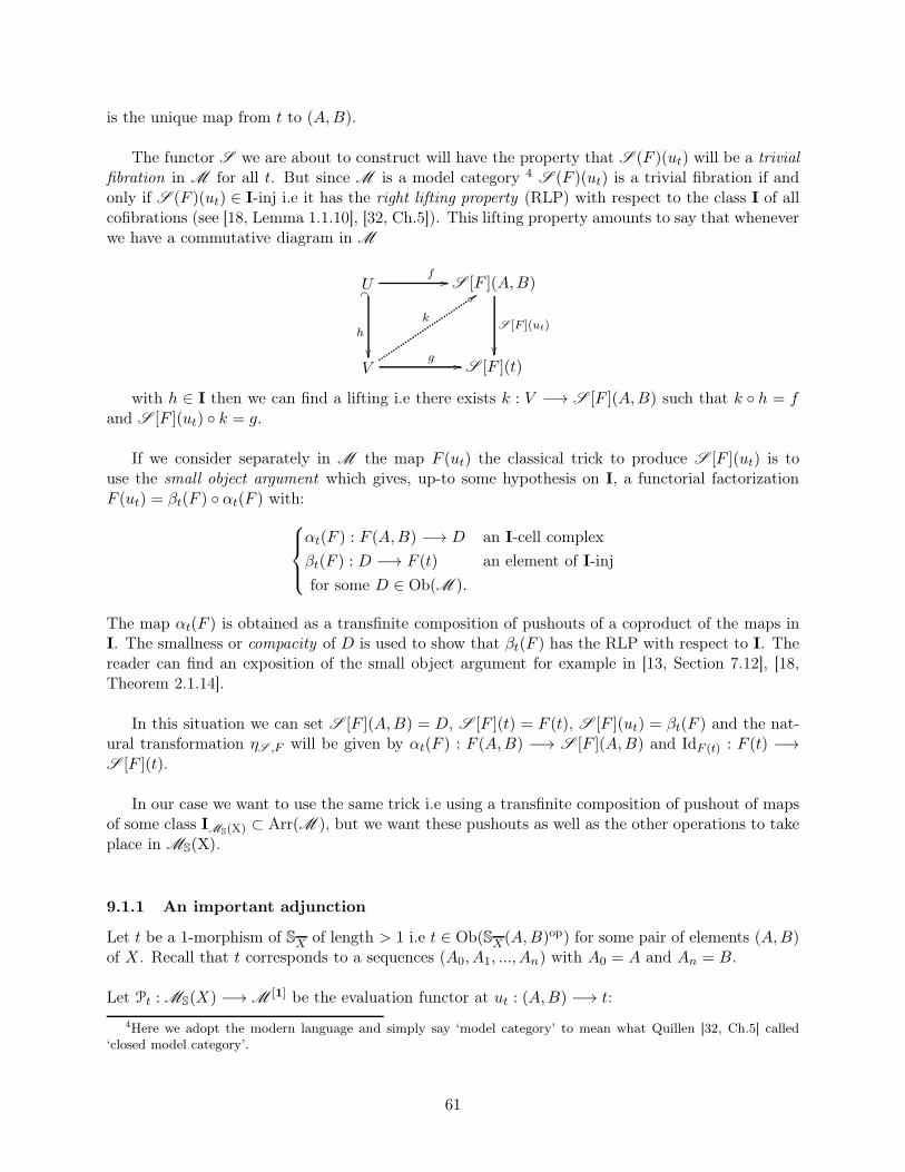
is the unique map from t to (A,B).

The functor S we are about to construct will have the property that S (F )(ut) will be a trivialfibration in M for all t. But since M is a model category 4 S (F )(ut) is a trivial fibration if andonly if S (F )(ut) ∈ I-inj i.e it has the right lifting property (RLP) with respect to the class I of allcofibrations (see [18, Lemma 1.1.10], [32, Ch.5]). This lifting property amounts to say that wheneverwe have a commutative diagram in M

U S [F ](A,B)

V S [F ](t)

f //_�

h

��

S [F ](ut)

��g //

k

::

with h ∈ I then we can find a lifting i.e there exists k : V −→ S [F ](A,B) such that k ◦ h = fand S [F ](ut) ◦ k = g.

If we consider separately in M the map F (ut) the classical trick to produce S [F ](ut) is touse the small object argument which gives, up-to some hypothesis on I, a functorial factorizationF (ut) = βt(F ) ◦ αt(F ) with:

αt(F ) : F (A,B) −→ D an I-cell complex

βt(F ) : D −→ F (t) an element of I-inj

for some D ∈ Ob(M ).

The map αt(F ) is obtained as a transfinite composition of pushouts of a coproduct of the maps inI. The smallness or compacity of D is used to show that βt(F ) has the RLP with respect to I. Thereader can find an exposition of the small object argument for example in [13, Section 7.12], [18,Theorem 2.1.14].

In this situation we can set S [F ](A,B) = D, S [F ](t) = F (t), S [F ](ut) = βt(F ) and the nat-ural transformation ηS ,F will be given by αt(F ) : F (A,B) −→ S [F ](A,B) and IdF (t) : F (t) −→S [F ](t).

In our case we want to use the same trick i.e using a transfinite composition of pushout of mapsof some class IMS(X) ⊂ Arr(M ), but we want these pushouts as well as the other operations to takeplace in MS(X).

9.1.1 An important adjunction

Let t be a 1-morphism of SX of length > 1 i.e t ∈ Ob(SX(A,B)op) for some pair of elements (A,B)of X. Recall that t corresponds to a sequences (A0, A1, ..., An) with A0 = A and An = B.

Let Pt : MS(X) −→M [1] be the evaluation functor at ut : (A,B) −→ t:

4Here we adopt the modern language and simply say ‘model category’ to mean what Quillen [32, Ch.5] called‘closed model category’.

61

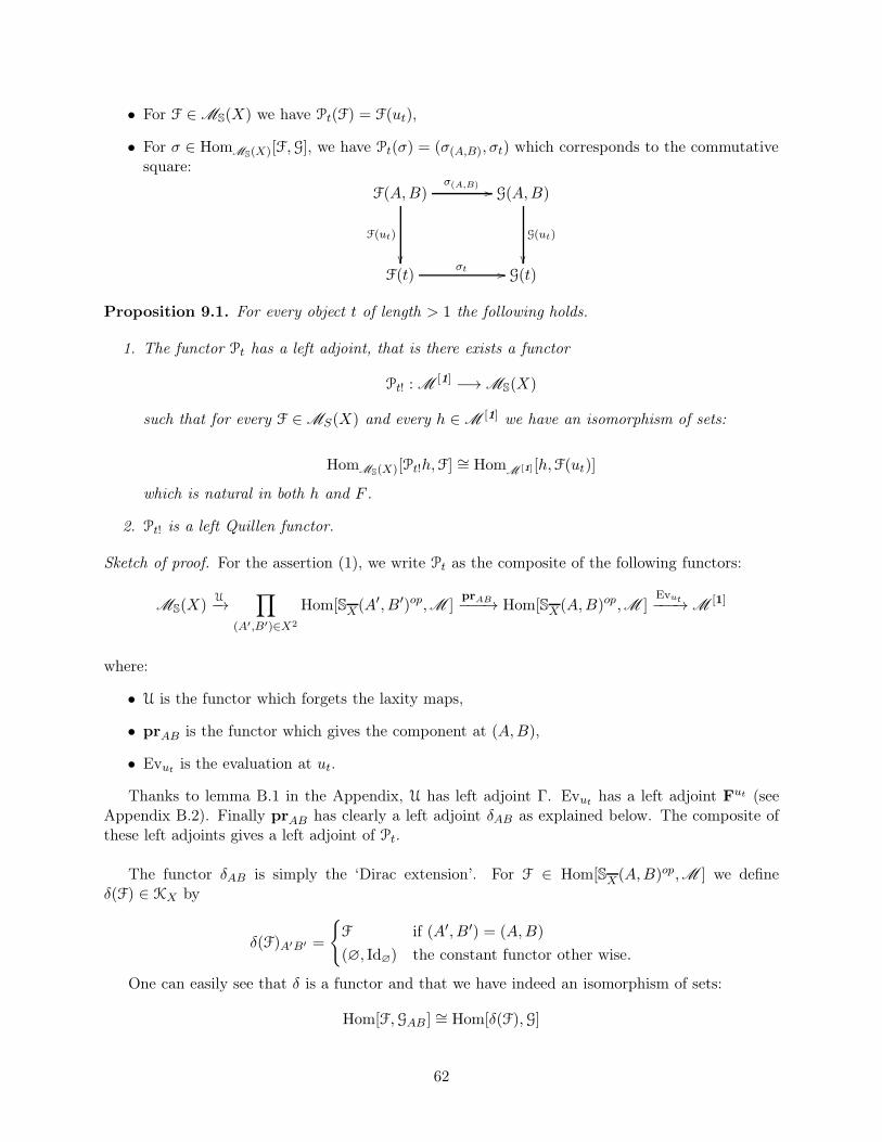
• For F ∈MS(X) we have Pt(F) = F(ut),

• For σ ∈ HomMS(X)[F,G], we have Pt(σ) = (σ(A,B), σt) which corresponds to the commutativesquare:

F(A,B) G(A,B)

F(t) G(t)

σ(A,B) //

F(ut)

��

G(ut)

��σt //

Proposition 9.1. For every object t of length > 1 the following holds.

1. The functor Pt has a left adjoint, that is there exists a functor

Pt! : M[1] −→MS(X)

such that for every F ∈MS(X) and every h ∈M [1] we have an isomorphism of sets:

HomMS(X)[Pt!h,F] ∼= HomM [1][h,F(ut)]

which is natural in both h and F .

2. Pt! is a left Quillen functor.

Sketch of proof. For the assertion (1), we write Pt as the composite of the following functors:

MS(X)U−→

∏

(A′,B′)∈X2

Hom[SX(A′, B′)op,M ]

prAB−−−→ Hom[SX(A,B)op,M ]Evut−−−→M

[1]

where:

• U is the functor which forgets the laxity maps,

• prAB is the functor which gives the component at (A,B),

• Evut is the evaluation at ut.

Thanks to lemma B.1 in the Appendix, U has left adjoint Γ. Evut has a left adjoint Fut (seeAppendix B.2). Finally prAB has clearly a left adjoint δAB as explained below. The composite ofthese left adjoints gives a left adjoint of Pt.

The functor δAB is simply the ‘Dirac extension’. For F ∈ Hom[SX(A,B)op,M ] we defineδ(F) ∈ KX by

δ(F)A′B′ =

{F if (A′, B′) = (A,B)

(∅, Id∅) the constant functor other wise.

One can easily see that δ is a functor and that we have indeed an isomorphism of sets:

Hom[F,GAB ] ∼= Hom[δ(F),G]

62

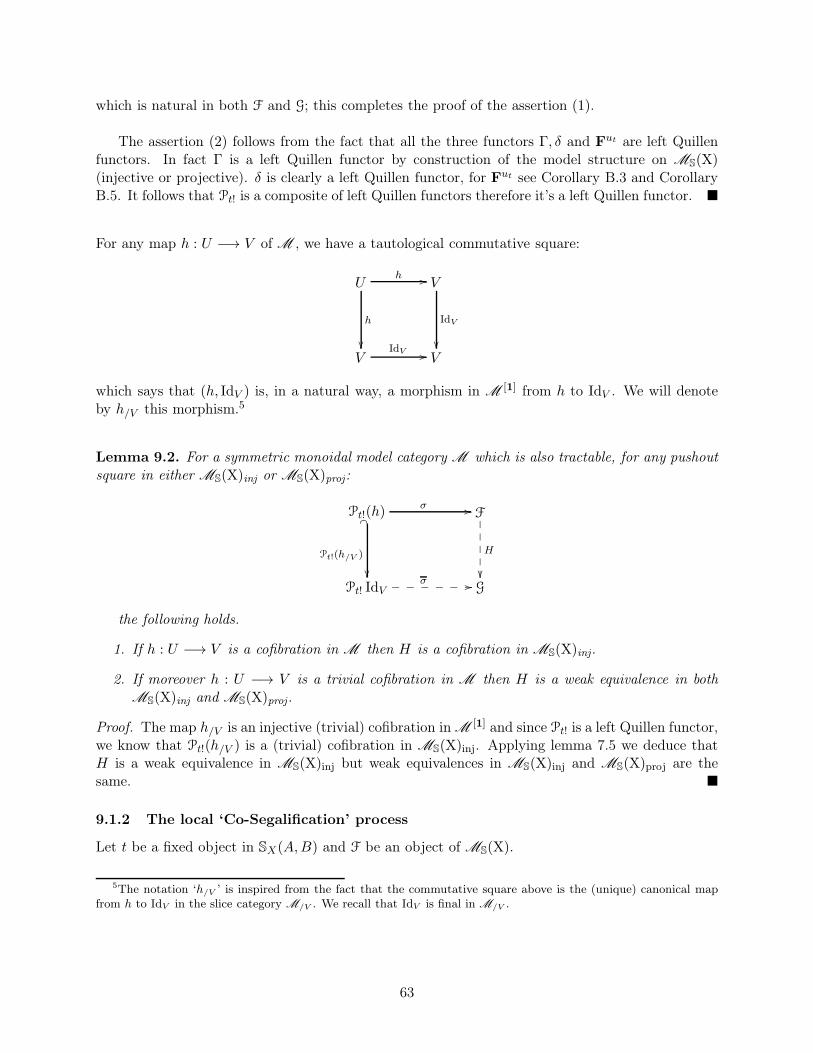
which is natural in both F and G; this completes the proof of the assertion (1).

The assertion (2) follows from the fact that all the three functors Γ, δ and Fut are left Quillenfunctors. In fact Γ is a left Quillen functor by construction of the model structure on MS(X)(injective or projective). δ is clearly a left Quillen functor, for Fut see Corollary B.3 and CorollaryB.5. It follows that Pt! is a composite of left Quillen functors therefore it’s a left Quillen functor. �

For any map h : U −→ V of M , we have a tautological commutative square:

U V

V V

h //

h

��

IdV

��IdV //

which says that (h, IdV ) is, in a natural way, a morphism in M [1] from h to IdV . We will denoteby h/V this morphism.5

Lemma 9.2. For a symmetric monoidal model category M which is also tractable, for any pushoutsquare in either MS(X)inj or MS(X)proj:

Pt!(h) F

Pt! IdV G

σ //_�

Pt!(h/V )

��

H

��✤✤✤✤✤

σ //❴❴❴❴❴❴

the following holds.

1. If h : U −→ V is a cofibration in M then H is a cofibration in MS(X)inj.

2. If moreover h : U −→ V is a trivial cofibration in M then H is a weak equivalence in bothMS(X)inj and MS(X)proj.

Proof. The map h/V is an injective (trivial) cofibration in M [1] and since Pt! is a left Quillen functor,we know that Pt!(h/V ) is a (trivial) cofibration in MS(X)inj. Applying lemma 7.5 we deduce thatH is a weak equivalence in MS(X)inj but weak equivalences in MS(X)inj and MS(X)proj are thesame. �

9.1.2 The local ‘Co-Segalification’ process

Let t be a fixed object in SX(A,B) and F be an object of MS(X).

5The notation ‘h/V ’ is inspired from the fact that the commutative square above is the (unique) canonical mapfrom h to IdV in the slice category M/V . We recall that IdV is final in M/V .

63

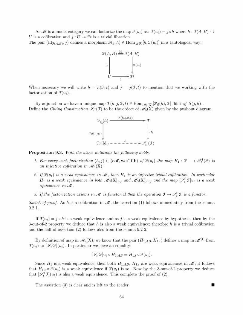
As M is a model category we can factorize the map F(ut) as: F(ut) = j◦h where h : F(A,B) →U is a cofibration and j : U ։ Ft is a trivial fibration.The pair (IdF(A,B), j) defines a morphism S(j, h) ∈ Hom

M [1] [h,F(ut)] in a tautological way:

F(A,B) F(A,B)

U Ft

Id

h

��

j//

F(ut)

��

When necessary we will write h = h(F, t) and j = j(F, t) to mention that we working with thefactorization of F(ut).

By adjunction we have a unique map T (h, j,F, t) ∈ HomMS(X)[Pt!(h),F] ‘lifiting’ S(j, h) .Define the Gluing Construction S 1

t (F) to be the object of MS(X) given by the pushout diagram

Pt!(h) F

Pt! IdU S 1t (F)

T (h,j,F,t) //_�

Pt!(h/U )

��

H1

��✤✤✤✤✤

α //❴❴❴❴❴❴❴❴

Proposition 9.3. With the above notations the following holds.

1. For every such factorization (h, j) ∈ (cof ,we∩fib) of F(ut) the map H1 : F −→ S 1t (F) is

an injective cofibration in MS(X).

2. If F(ut) is a weak equivalence in M , then H1 is an injective trivial cofibration. In particularH1 is a weak equivalence in both MS(X)inj and MS(X)proj and the map [S 1

t F]ut is a weakequivalence in M .

3. If the factorization axioms in M is functorial then the operation F 7→ S 1t F is a functor.

Sketch of proof. As h is a cofibration in M , the assertion (1) follows immediately from the lemma9.2 1.

If F(ut) = j ◦ h is a weak equivalence and as j is a weak equivalence by hypothesis, then by the3-out-of-2 property we deduce that h is also a weak equivalence; therefore h is a trivial cofibrationand the half of assertion (2) follows also from the lemma 9.2 2.

By definition of map in MS(X), we know that the pair (H1,AB ,H1,t) defines a map in M [1] fromF(ut) to [S 1

t F](ut). In particular we have an equality:

[S 1t F]ut ◦H1,AB = H1,t ◦ F(ut).

Since H1 is a weak equivalence, then both H1,AB, H1,t are weak equivalences in M ; it followsthat H1,t ◦ F(ut) is a weak equivalence if F(ut) is so. Now by the 3-out-of-2 property we deducethat [S 1

t F](ut) is also a weak equivalence. This complete the proof of (2).

The assertion (3) is clear and is left to the reader. �

64

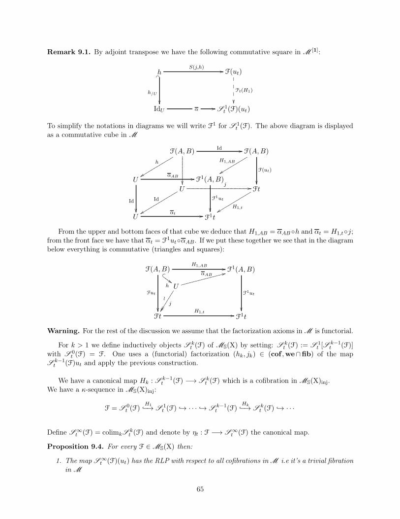
Remark 9.1. By adjoint transpose we have the following commutative square in M [1]:

h F(ut)

IdU S 1t (F)(ut)

S(j,h) //_�

h/U

��

Pt(H1)

��✤✤

✤

✤

α //

To simplify the notations in diagrams we will write F1 for S 1t (F). The above diagram is displayed

as a commutative cube in M

F(A,B) F(A,B)

U Ft

Id //

��

F(ut)

��j //U F1(A,B)

U F1t

αAB //

Id

��

F1ut

��αt //

h

yyrrrrrrrrrrrr

H1,AB

yyrrrrrrrrrr

Id

yyrrrrrrrrrrrrrr

H1,tyyrrrrrrrrrrrr

From the upper and bottom faces of that cube we deduce that H1,AB = αAB ◦h and αt = H1,t◦j;from the front face we have that αt = F1ut◦αAB . If we put these together we see that in the diagrambelow everything is commutative (triangles and squares):

F(A,B) F1(A,B)

Ft F1t

U

H1,AB //

Fut

��

F1ut

��H1,t //

� r

h$$❍❍

❍❍

j≀

����☛☛☛☛☛☛☛☛

αAB33❣❣❣❣❣❣❣❣❣❣❣❣❣❣❣

Warning. For the rest of the discussion we assume that the factorization axioms in M is functorial.

For k > 1 we define inductively objects S kt (F) of MS(X) by setting: S k

t (F) := S 1t [S

k−1t (F)]

with S 0t (F) = F. One uses a (functorial) factorization (hk, jk) ∈ (cof ,we∩fib) of the map

Sk−1t (F)ut and apply the previous construction.

We have a canonical map Hk : Sk−1t (F) −→ S k

t (F) which is a cofibration in MS(X)inj.We have a κ-sequence in MS(X)inj:

F = S0t (F)

H1−→ S

1t (F) → · · · → S

k−1t (F)

Hk−→ S

kt (F) → · · ·

Define S ∞t (F) = colimkS

kt (F) and denote by ηt : F −→ S ∞

t (F) the canonical map.

Proposition 9.4. For every F ∈MS(X) then:

1. The map S ∞t (F)(ut) has the RLP with respect to all cofibrations in M i.e it’s a trivial fibration

in M

65

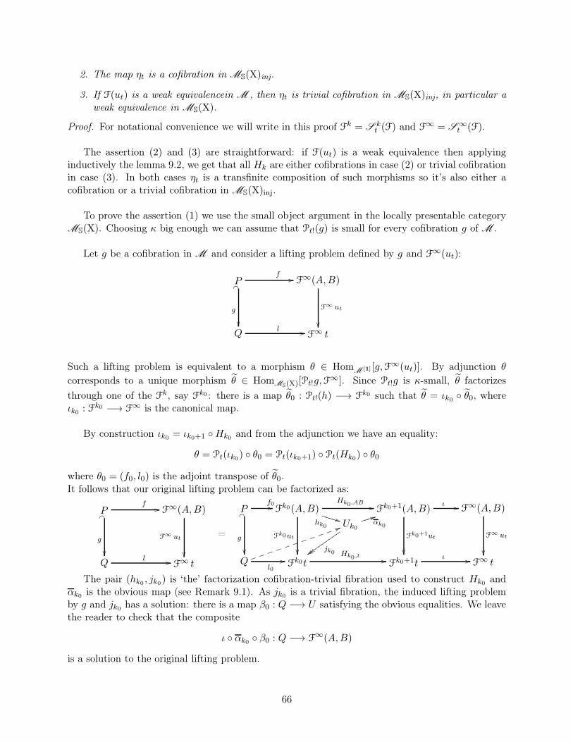
2. The map ηt is a cofibration in MS(X)inj.

3. If F(ut) is a weak equivalencein M , then ηt is trivial cofibration in MS(X)inj, in particular aweak equivalence in MS(X).

Proof. For notational convenience we will write in this proof Fk = S kt (F) and F∞ = S ∞

t (F).

The assertion (2) and (3) are straightforward: if F(ut) is a weak equivalence then applyinginductively the lemma 9.2, we get that all Hk are either cofibrations in case (2) or trivial cofibrationin case (3). In both cases ηt is a transfinite composition of such morphisms so it’s also either acofibration or a trivial cofibration in MS(X)inj.

To prove the assertion (1) we use the small object argument in the locally presentable categoryMS(X). Choosing κ big enough we can assume that Pt!(g) is small for every cofibration g of M .

Let g be a cofibration in M and consider a lifting problem defined by g and F∞(ut):

P F∞(A,B)

Q F∞ t

f //_�

g

��

F∞ ut

��l //

Such a lifting problem is equivalent to a morphism θ ∈ HomM [1] [g,F∞(ut)]. By adjunction θ

corresponds to a unique morphism θ ∈ HomMS(X)[Pt!g,F∞]. Since Pt!g is κ-small, θ factorizes

through one of the Fk, say Fk0 : there is a map θ0 : Pt!(h) −→ Fk0 such that θ = ιk0 ◦ θ0, whereιk0 : Fk0 −→ F∞ is the canonical map.

By construction ιk0 = ιk0+1 ◦Hk0 and from the adjunction we have an equality:

θ = Pt(ιk0) ◦ θ0 = Pt(ιk0+1) ◦ Pt(Hk0) ◦ θ0

where θ0 = (f0, l0) is the adjoint transpose of θ0.It follows that our original lifting problem can be factorized as:

P F∞(A,B)

Q F∞ t

f //_�

g

��

F∞ ut

��l //

=

P Fk0(A,B)

Q Fk0t

Uk0

f0//_�

g

��

Fk0ut

��

l0//

Fk0+1(A,B)

Fk0+1t

Fk0+1ut

��

Hk0,AB //

Hk0,t //

F∞(A,B)

F∞ t

F∞ ut

��

ι //

ι //

hk0**❯❯❯❯

❯

jk0zzzz✉✉✉✉✉✉✉✉✉

αk0

44✐✐✐✐55❥❥❥❥❥❥❥❥❥❥❥

The pair (hk0 , jk0) is ‘the’ factorization cofibration-trivial fibration used to construct Hk0 andαk0 is the obvious map (see Remark 9.1). As jk0 is a trivial fibration, the induced lifting problemby g and jk0 has a solution: there is a map β0 : Q −→ U satisfying the obvious equalities. We leavethe reader to check that the composite

ι ◦ αk0 ◦ β0 : Q −→ F∞(A,B)

is a solution to the original lifting problem.

66

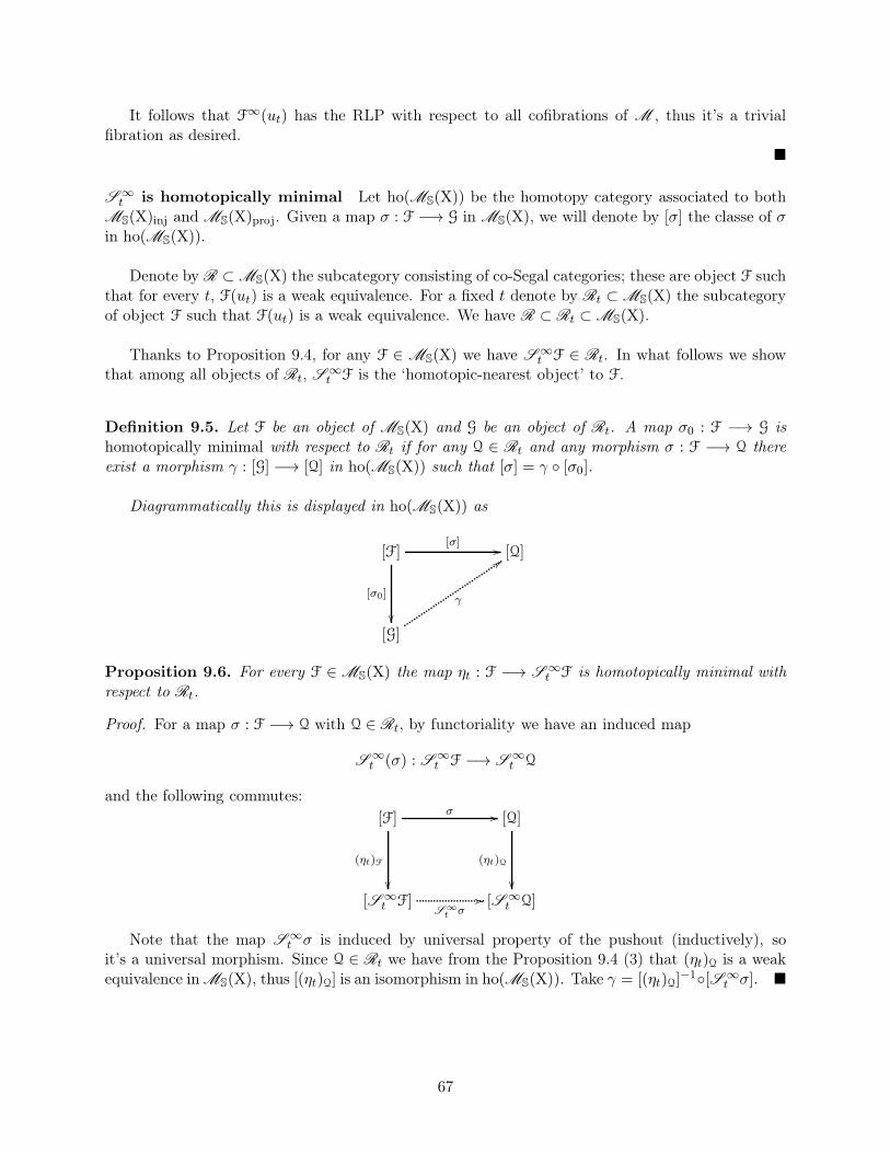
It follows that F∞(ut) has the RLP with respect to all cofibrations of M , thus it’s a trivialfibration as desired.

�

S ∞t is homotopically minimal Let ho(MS(X)) be the homotopy category associated to both

MS(X)inj and MS(X)proj. Given a map σ : F −→ G in MS(X), we will denote by [σ] the classe of σin ho(MS(X)).

Denote by R ⊂MS(X) the subcategory consisting of co-Segal categories; these are object F suchthat for every t, F(ut) is a weak equivalence. For a fixed t denote by Rt ⊂MS(X) the subcategoryof object F such that F(ut) is a weak equivalence. We have R ⊂ Rt ⊂MS(X).

Thanks to Proposition 9.4, for any F ∈ MS(X) we have S ∞t F ∈ Rt. In what follows we show

that among all objects of Rt, S ∞t F is the ‘homotopic-nearest object’ to F.

Definition 9.5. Let F be an object of MS(X) and G be an object of Rt. A map σ0 : F −→ G ishomotopically minimal with respect to Rt if for any Q ∈ Rt and any morphism σ : F −→ Q thereexist a morphism γ : [G] −→ [Q] in ho(MS(X)) such that [σ] = γ ◦ [σ0].

Diagrammatically this is displayed in ho(MS(X)) as

[F] [Q]

[G]

[σ] //

[σ0]

��

γ

::

Proposition 9.6. For every F ∈MS(X) the map ηt : F −→ S ∞t F is homotopically minimal with

respect to Rt.

Proof. For a map σ : F −→ Q with Q ∈ Rt, by functoriality we have an induced map

S∞t (σ) : S

∞t F −→ S

∞t Q

and the following commutes:

[F] [Q]

[S ∞t F] [S ∞

t Q]

σ //

(ηt)F

��

S ∞t σ

//

(ηt)Q

��

Note that the map S ∞t σ is induced by universal property of the pushout (inductively), so

it’s a universal morphism. Since Q ∈ Rt we have from the Proposition 9.4 (3) that (ηt)Q is a weakequivalence in MS(X), thus [(ηt)Q] is an isomorphism in ho(MS(X)). Take γ = [(ηt)Q]

−1◦[S ∞t σ]. �

67

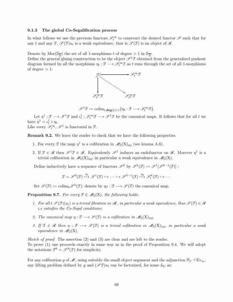
9.1.3 The global Co-Segalification process

In what follows we use the previous functors S ∞t to construct the desired functor S such that for

any t and any F, S (F)ut is a weak equivalence, that is S (F) is an object of R.

Denote by Mor(SX) the set of all 1-morphisms t of degree > 1 in SX .Define the general gluing construction to be the object S 1F obtained from the generalized pushoutdiagram formed by all the morphisms ηt : F −→ S ∞

t F as t runs through the set of all 1-morphismsof degree > 1:

F S ∞t F

S ∞t′ F S ∞

t′′ F

� � //_�

��

� r

%%❏❏❏

❏❏❏❏

❏❏❏❏

❏❏❏❏

❏

S1F := colimt,deg(t)>1{ηt : F −→ S

∞t F}.

Let η1 : F −→ S 1F and ι1t : S ∞t F −→ S 1F be the canonical maps. It follows that for all t we

have η1 = ι1t ◦ ηt.Like every S ∞

t , S 1 is functorial in F.

Remark 9.2. We leave the reader to check that we have the following properties.

1. For every F the map η1 is a cofibration in MS(X)inj (see lemma A.6).

2. If F ∈ R then S 1F ∈ R. Equivalently S 1 induces an endofunctor on R. Morever η1 is atrivial cofibration in MS(X)inj; in particular a weak equivalence in MS(X).

Define inductively have a sequence of functors S k by S k(F) := S 1[S k−1(F)] :

F = S0(F)

η1−→ S

1(F) → · · · → Sk−1(F)

ηk−→ S

kt (F) → · · ·

Set S (F) := colimkSk(F); denote by ηF : F −→ S (F) the canonical map.

Proposition 9.7. For every F ∈MS(X), the following holds.

1. For all t S (F)(ut) is a trivial fibration in M , in particular a weak equivalence, thus S (F) ∈ R

i.e satisfies the Co-Segal conditions.

2. The canonical map η : F −→ S (F) is a cofibration in MS(X)inj.

3. If F ∈ R then η : F −→ S (F) is a trivial cofibration in MS(X)inj, in particular a weakequivalence in MS(X).

Sketch of proof. The assertion (2) and (3) are clear and are left to the reader.To prove (1) one proceeds exactly in same way as in the proof of Proposition 9.4. We will adoptthe notations Fk = S k(F) for simplicity.

For any cofibration g of M , using suitably the small object argument and the adjunction Pt! ⊣ Evut ,any lifting problem defined by g and (S F)ut can be factorized, for some k0, as:

68

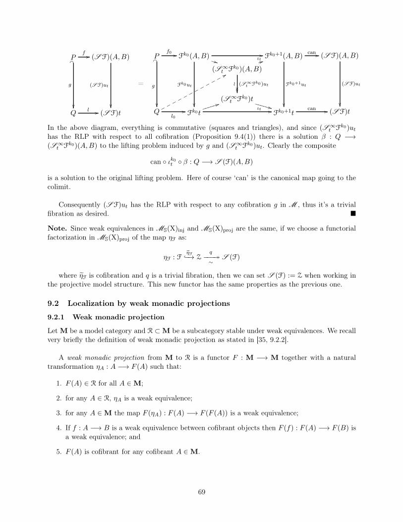
P (S F)(A,B)

Q (S F)t

f //_�

g

��

(S F)ut

��l //

=

P Fk0(A,B)

Q Fk0t

(S ∞t Fk0)(A,B)

(S ∞t Fk0)t

f0 //_�

g

��

Fk0ut

��

l0//

**❯❯

44✐✐✐✐✐✐

Fk0+1(A,B)

Fk0+1t

Fk0+1ut

��

//

//

(SF)(A,B)

(SF)t

(S F)ut

��

can //

can //

(S ∞t Fk0 )ut≀

����

ιt 33❤❤

ιt ++❱❱❱❱❱❱

88♣♣

♣♣

♣♣

♣♣

♣♣

♣♣

In the above diagram, everything is commutative (squares and triangles), and since (S ∞t Fk0)ut

has the RLP with respect to all cofibration (Proposition 9.4(1)) there is a solution β : Q −→(S ∞

t Fk0)(A,B) to the lifting problem induced by g and (S ∞t Fk0)ut. Clearly the composite

can ◦ ιk0t ◦ β : Q −→ S (F)(A,B)

is a solution to the original lifting problem. Here of course ‘can’ is the canonical map going to thecolimit.

Consequently (SF)ut has the RLP with respect to any cofibration g in M , thus it’s a trivialfibration as desired. �

Note. Since weak equivalences in MS(X)inj and MS(X)proj are the same, if we choose a functorialfactorization in MS(X)proj of the map ηF as:

ηF : FηF−→ Z

q−−−։

∼S (F)

where ηF is cofibration and q is a trivial fibration, then we can set S (F) := Z when working inthe projective model structure. This new functor has the same properties as the previous one.

9.2 Localization by weak monadic projections

9.2.1 Weak monadic projection

Let M be a model category and R ⊂M be a subcategory stable under weak equivalences. We recallvery briefly the definition of weak monadic projection as stated in [35, 9.2.2].

A weak monadic projection from M to R is a functor F : M −→ M together with a naturaltransformation ηA : A −→ F (A) such that:

1. F (A) ∈ R for all A ∈M;

2. for any A ∈ R, ηA is a weak equivalence;

3. for any A ∈M the map F (ηA) : F (A) −→ F (F (A)) is a weak equivalence;

4. If f : A −→ B is a weak equivalence between cofibrant objects then F (f) : F (A) −→ F (B) isa weak equivalence; and

5. F (A) is cofibrant for any cofibrant A ∈M.

69

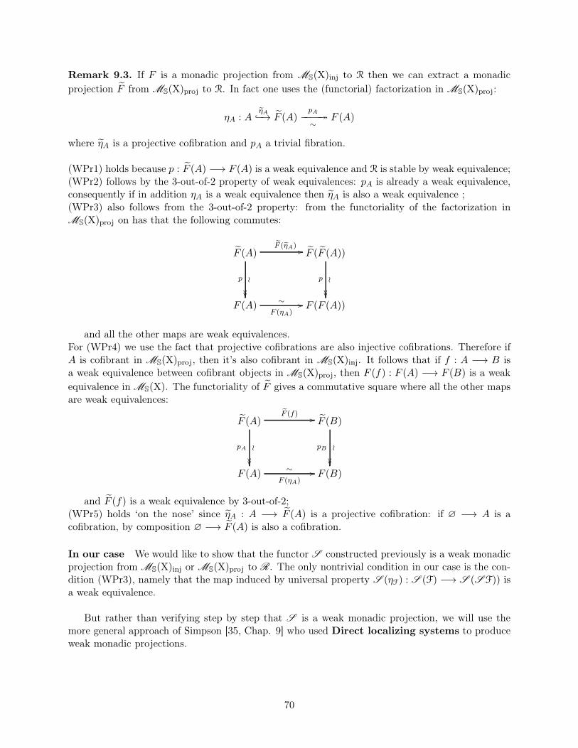
Remark 9.3. If F is a monadic projection from MS(X)inj to R then we can extract a monadic

projection F from MS(X)proj to R. In fact one uses the (functorial) factorization in MS(X)proj:

ηA : AηA−→ F (A)

pA−−−−։

∼F (A)

where ηA is a projective cofibration and pA a trivial fibration.

(WPr1) holds because p : F (A) −→ F (A) is a weak equivalence and R is stable by weak equivalence;(WPr2) follows by the 3-out-of-2 property of weak equivalences: pA is already a weak equivalence,consequently if in addition ηA is a weak equivalence then ηA is also a weak equivalence ;(WPr3) also follows from the 3-out-of-2 property: from the functoriality of the factorization inMS(X)proj on has that the following commutes:

F (A) F (F (A))

F (A) F (F (A))

F (ηA) //

p ≀

����

F (ηA)

∼ //

p ≀

����

and all the other maps are weak equivalences.For (WPr4) we use the fact that projective cofibrations are also injective cofibrations. Therefore ifA is cofibrant in MS(X)proj, then it’s also cofibrant in MS(X)inj. It follows that if f : A −→ B isa weak equivalence between cofibrant objects in MS(X)proj, then F (f) : F (A) −→ F (B) is a weak

equivalence in MS(X). The functoriality of F gives a commutative square where all the other mapsare weak equivalences:

F (A) F (B)

F (A) F (B)

F (f) //

pA ≀

����

F (ηA)

∼ //

pB ≀

����

and F (f) is a weak equivalence by 3-out-of-2;(WPr5) holds ‘on the nose’ since ηA : A −→ F (A) is a projective cofibration: if ∅ −→ A is acofibration, by composition ∅ −→ F (A) is also a cofibration.

In our case We would like to show that the functor S constructed previously is a weak monadicprojection from MS(X)inj or MS(X)proj to R. The only nontrivial condition in our case is the con-dition (WPr3), namely that the map induced by universal property S (ηF) : S (F) −→ S (SF)) isa weak equivalence.

But rather than verifying step by step that S is a weak monadic projection, we will use themore general approach of Simpson [35, Chap. 9] who used Direct localizing systems to produceweak monadic projections.

70

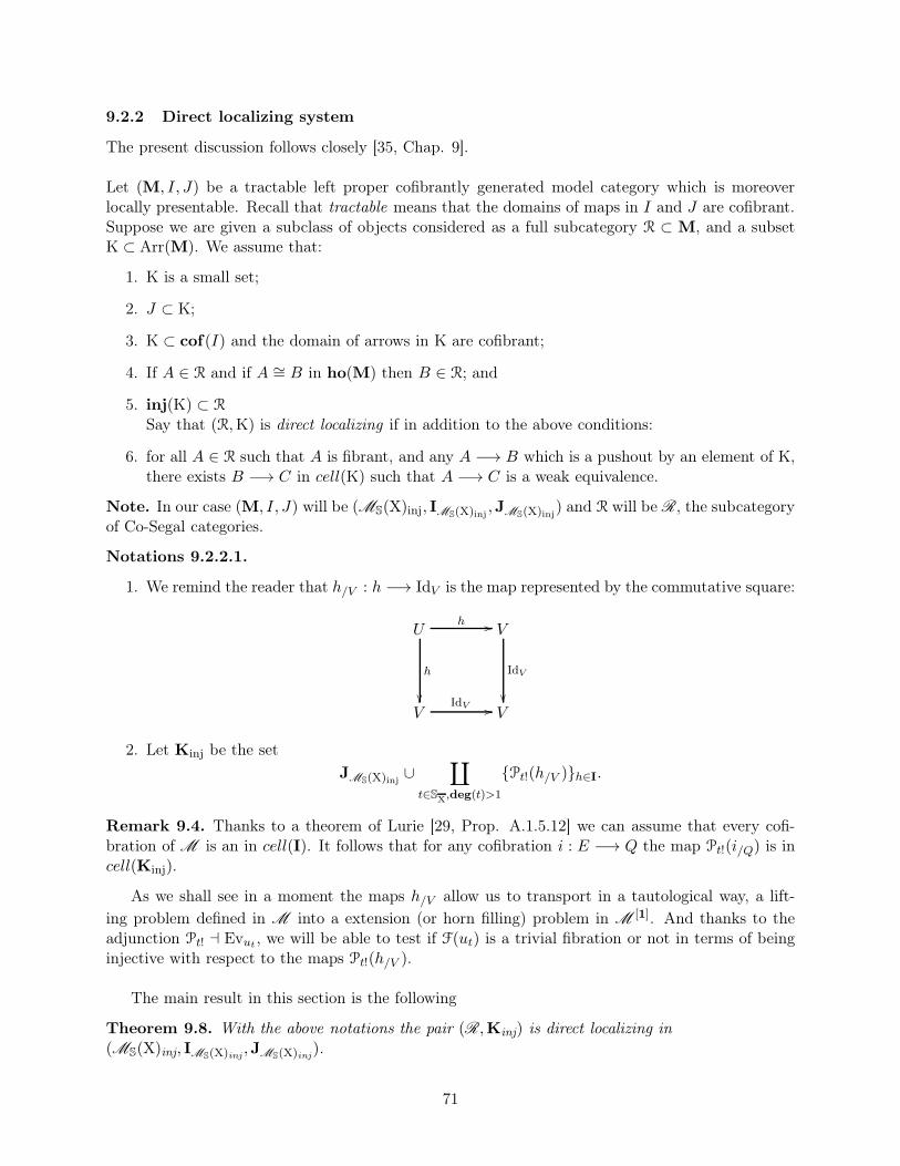
9.2.2 Direct localizing system

The present discussion follows closely [35, Chap. 9].

Let (M, I, J) be a tractable left proper cofibrantly generated model category which is moreoverlocally presentable. Recall that tractable means that the domains of maps in I and J are cofibrant.Suppose we are given a subclass of objects considered as a full subcategory R ⊂ M, and a subsetK ⊂ Arr(M). We assume that:

1. K is a small set;

2. J ⊂ K;

3. K ⊂ cof(I) and the domain of arrows in K are cofibrant;

4. If A ∈ R and if A ∼= B in ho(M) then B ∈ R; and

5. inj(K) ⊂ R

Say that (R,K) is direct localizing if in addition to the above conditions:

6. for all A ∈ R such that A is fibrant, and any A −→ B which is a pushout by an element of K,there exists B −→ C in cell(K) such that A −→ C is a weak equivalence.

Note. In our case (M, I, J) will be (MS(X)inj, IMS(X)inj,JMS(X)inj

) and R will be R, the subcategoryof Co-Segal categories.

Notations 9.2.2.1.

1. We remind the reader that h/V : h −→ IdV is the map represented by the commutative square:

U V

V V

h //

h

��

IdV

��IdV //

2. Let Kinj be the set

JMS(X)inj∪

∐

t∈SX,deg(t)>1

{Pt!(h/V )}h∈I.

Remark 9.4. Thanks to a theorem of Lurie [29, Prop. A.1.5.12] we can assume that every cofi-bration of M is an in cell(I). It follows that for any cofibration i : E −→ Q the map Pt!(i/Q) is incell(Kinj).

As we shall see in a moment the maps h/V allow us to transport in a tautological way, a lift-

ing problem defined in M into a extension (or horn filling) problem in M [1]. And thanks to theadjunction Pt! ⊣ Evut , we will be able to test if F(ut) is a trivial fibration or not in terms of beinginjective with respect to the maps Pt!(h/V ).

The main result in this section is the following

Theorem 9.8. With the above notations the pair (R,Kinj) is direct localizing in(MS(X)inj, IMS(X)inj

,JMS(X)inj).

71

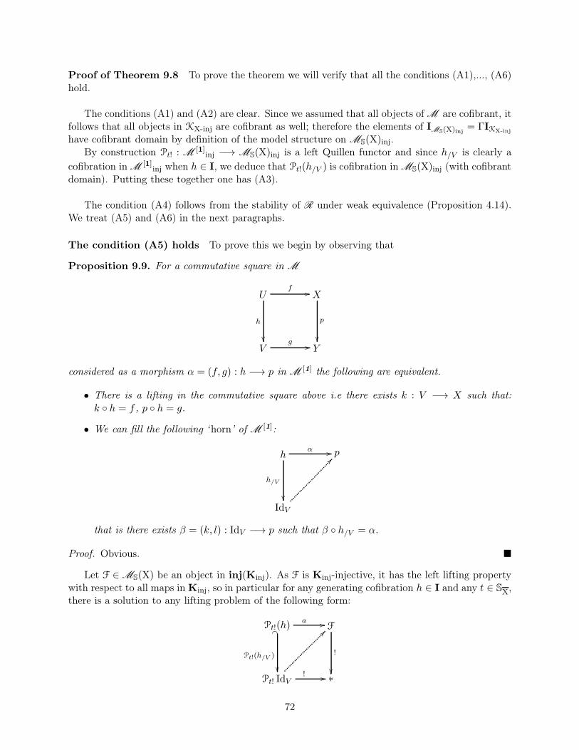
Proof of Theorem 9.8 To prove the theorem we will verify that all the conditions (A1),..., (A6)hold.

The conditions (A1) and (A2) are clear. Since we assumed that all objects of M are cofibrant, itfollows that all objects in KX-inj are cofibrant as well; therefore the elements of IMS(X)inj

= ΓIKX-inj

have cofibrant domain by definition of the model structure on MS(X)inj.By construction Pt! : M [1]

inj −→ MS(X)inj is a left Quillen functor and since h/V is clearly a

cofibration in M [1]inj when h ∈ I, we deduce that Pt!(h/V ) is cofibration in MS(X)inj (with cofibrant

domain). Putting these together one has (A3).

The condition (A4) follows from the stability of R under weak equivalence (Proposition 4.14).We treat (A5) and (A6) in the next paragraphs.

The condition (A5) holds To prove this we begin by observing that

Proposition 9.9. For a commutative square in M

U X

V Y

f //

h

��

p

��g //

considered as a morphism α = (f, g) : h −→ p in M [1] the following are equivalent.

• There is a lifting in the commutative square above i.e there exists k : V −→ X such that:k ◦ h = f , p ◦ h = g.

• We can fill the following ‘horn’ of M [1]:

h p

IdV

α //

h/V

��

??

that is there exists β = (k, l) : IdV −→ p such that β ◦ h/V = α.

Proof. Obvious. �

Let F ∈MS(X) be an object in inj(Kinj). As F is Kinj-injective, it has the left lifting propertywith respect to all maps in Kinj, so in particular for any generating cofibration h ∈ I and any t ∈ SX,there is a solution to any lifting problem of the following form:

Pt!(h) F

Pt! IdV ∗

a //_�

Pt!(h/V )

��

!

��! //

??

72

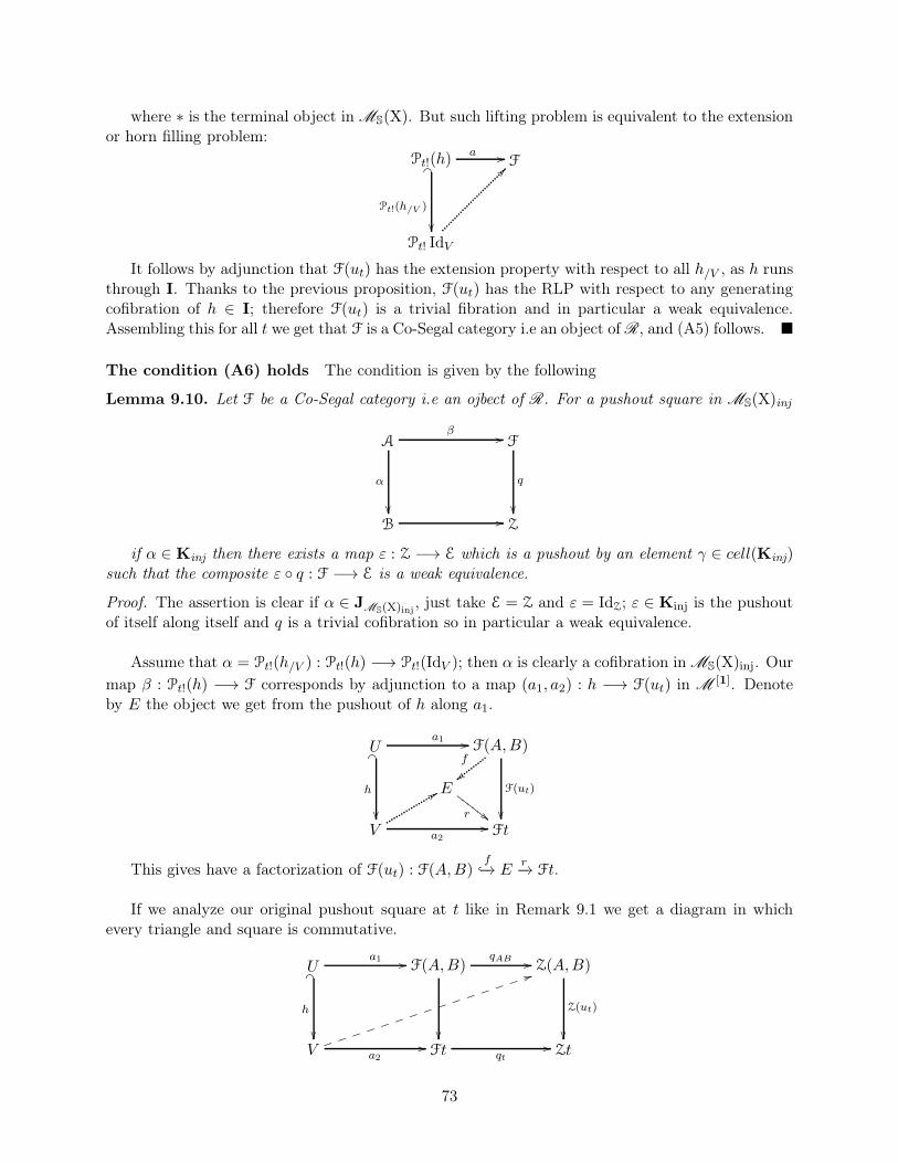
where ∗ is the terminal object in MS(X). But such lifting problem is equivalent to the extensionor horn filling problem:

Pt!(h) F

Pt! IdV

a //_�

Pt!(h/V )

��

??

It follows by adjunction that F(ut) has the extension property with respect to all h/V , as h runsthrough I. Thanks to the previous proposition, F(ut) has the RLP with respect to any generatingcofibration of h ∈ I; therefore F(ut) is a trivial fibration and in particular a weak equivalence.Assembling this for all t we get that F is a Co-Segal category i.e an object of R, and (A5) follows. �

The condition (A6) holds The condition is given by the following

Lemma 9.10. Let F be a Co-Segal category i.e an ojbect of R. For a pushout square in MS(X)inj

A F

B Z

β //

α

��//

q

��

if α ∈ Kinj then there exists a map ε : Z −→ E which is a pushout by an element γ ∈ cell(Kinj)such that the composite ε ◦ q : F −→ E is a weak equivalence.

Proof. The assertion is clear if α ∈ JMS(X)inj, just take E = Z and ε = IdZ; ε ∈ Kinj is the pushout

of itself along itself and q is a trivial cofibration so in particular a weak equivalence.

Assume that α = Pt!(h/V ) : Pt!(h) −→ Pt!(IdV ); then α is clearly a cofibration in MS(X)inj. Our

map β : Pt!(h) −→ F corresponds by adjunction to a map (a1, a2) : h −→ F(ut) in M [1]. Denoteby E the object we get from the pushout of h along a1.

U F(A,B)

V Ft

E

a1 //_�

h

��

a2//

F(ut)

��

f

{{88

r ##❋❋❋

❋❋❋

This gives have a factorization of F(ut) : F(A,B)f−→ E

r−→ Ft.

If we analyze our original pushout square at t like in Remark 9.1 we get a diagram in whichevery triangle and square is commutative.

U F(A,B)

V Ft

Z(A,B)

Zt

a1 //_�

h

��

a2//��

qAB //

qt//

Z(ut)

��

44❥❥❥❥❥❥❥❥❥❥❥❥❥❥❥

73

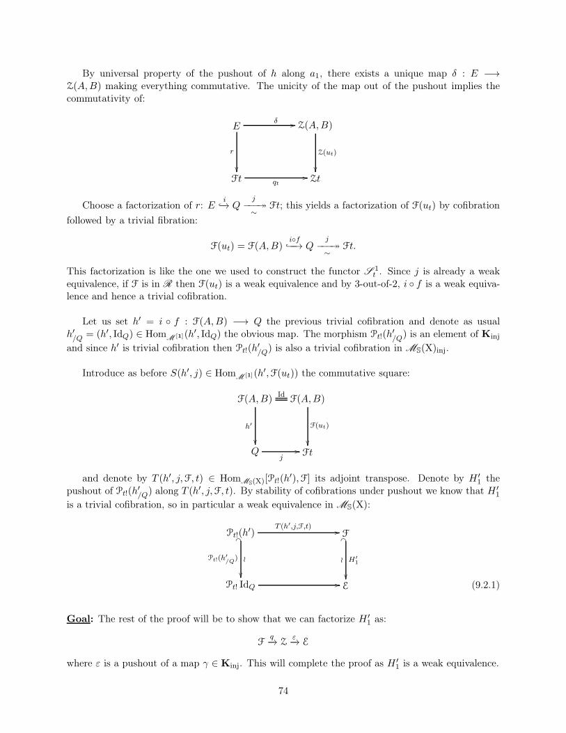
By universal property of the pushout of h along a1, there exists a unique map δ : E −→Z(A,B) making everything commutative. The unicity of the map out of the pushout implies thecommutativity of:

E Z(A,B)

Ft Zt

δ //

r

��

qt//

Z(ut)

��

Choose a factorization of r: Ei−→ Q

j−−−։

∼Ft; this yields a factorization of F(ut) by cofibration

followed by a trivial fibration:

F(ut) = F(A,B)i◦f−−→ Q

j−−−։

∼Ft.

This factorization is like the one we used to construct the functor S 1t . Since j is already a weak

equivalence, if F is in R then F(ut) is a weak equivalence and by 3-out-of-2, i ◦ f is a weak equiva-lence and hence a trivial cofibration.

Let us set h′ = i ◦ f : F(A,B) −→ Q the previous trivial cofibration and denote as usualh′/Q = (h′, IdQ) ∈ Hom

M [1](h′, IdQ) the obvious map. The morphism Pt!(h′/Q) is an element of Kinj

and since h′ is trivial cofibration then Pt!(h′/Q) is also a trivial cofibration in MS(X)inj.

Introduce as before S(h′, j) ∈ HomM [1](h′,F(ut)) the commutative square:

F(A,B) F(A,B)

Q Ft

Id

h′

��

j//

F(ut)

��

and denote by T (h′, j,F, t) ∈ HomMS(X)[Pt!(h′),F] its adjoint transpose. Denote by H ′

1 thepushout of Pt!(h

′/Q) along T (h′, j,F, t). By stability of cofibrations under pushout we know that H ′

1

is a trivial cofibration, so in particular a weak equivalence in MS(X):

Pt!(h′) F

Pt! IdQ E

T (h′,j,F,t) //_�

Pt!(h′/Q

) ≀

��

_�

H′1≀

��// (9.2.1)

Goal: The rest of the proof will be to show that we can factorize H ′1 as:

Fq−→ Z

ε−→ E

where ε is a pushout of a map γ ∈ Kinj. This will complete the proof as H ′1 is a weak equivalence.

74

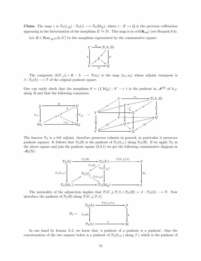
Claim. The map γ is Pt!(i/Q) : Pt!(i) −→ Pt!(IdQ), where i : E → Q is the previous cofibration

appearing in the factorization of the morphism Er−→ Ft. This map is in cell(Kinj) (see Remark 9.4).

Let R ∈ HomM [1](h, h′) be the morphism represented by the commutative square:

U F(A,B)

V Q

E

a1 //

h

��

g//

h′

��<<

""

��

The composite S(h′, j) ◦ R : h −→ F(ut) is the map (a1, a2) whose adjoint transpose isβ : Pt!(h) −→ F of the original pushout square.

One can easily check that the morphism θ = (f, IdQ) : h′ −→ i is the pushout in M [1] of h/Valong R and that the following commutes:

h h′

IdV IdQ

i

R //_�

h/V

��

_�

h′/Q≀

��//

77 � u

i/Q ((◗◗◗◗◗

◗◗◗◗

θ

ww =

U F(A,B)

V Q

a1 //

��

h′

��//

V Q

V Q

//

Id

�� ��//

hrrrrrr

yyrrrrrr h′

rrrrr

yyrrrrr

Idrrrrrr

yyrrrrrr Id

rrrrrr

yyrrrrrr

E

Q

i

��

i!!❈

❈❈

!!❈❈❈

33

33

rr

rr

The functor Pt! is a left adjoint, therefore preserves colimits in general, in particular it preservespushout squares. It follows that Pt!(θ) is the pushout of Pt!(h/V ) along Pt!(R). If we apply Pt! inthe above square and join the pushout square (9.2.1) we get the following commutative diagram inMS(X):

Pt!(h) Pt!(h′)

Pt!(IdV ) Pt!(IdQ)

Pt!(i)

Pt!(R) //_�

Pt!(h/V )

��

Pt!(h′/Q

)

��//

99 � sPt!(i/Q)

&&▲▲▲▲

▲▲▲

Pt!(θ)

yy

F

E

H1

��

T (h′,j,F,t) //

//

The naturality of the adjunction implies that T (h′, j,F, t) ◦ Pt!(R) = β : Pt!(h) −→ F. Nowintroduce the pushout of Pt!(θ) along T (h′, j,F, t):

D1 =

Pt!(h) F

Pt!(i) M

T (h′,j,F,t) //_�

Pt!(θ)

��

_�

g

��ξ //

In one hand by lemma A.2, we know that ‘a pushout of a pushout is a pushout’, thus theconcatenation of the two squares below is a pushout of Pt!(h/V ) along β ( which is the pushout of

75

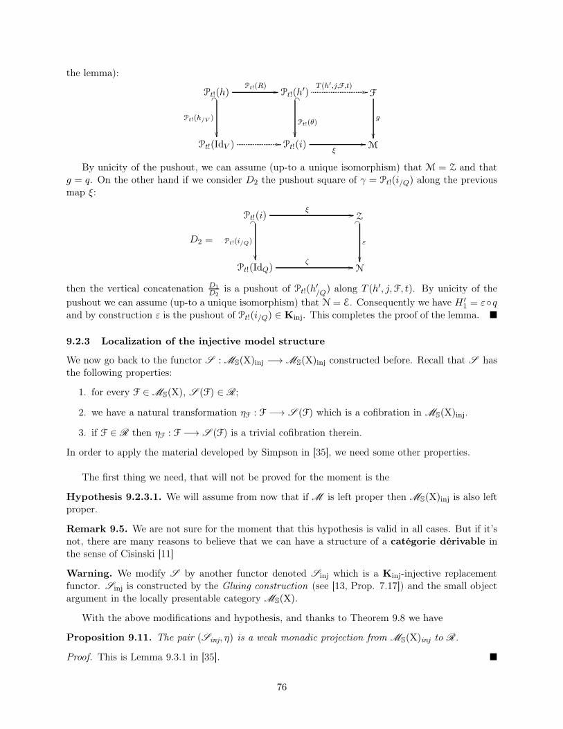
the lemma):

Pt!(h) Pt!(h′)

Pt!(IdV ) Pt!(i)

Pt!(R) //_�

Pt!(h/V )

��

� _

Pt!(θ)

��//

F

M

g

��

T (h′,j,F,t) //

ξ//

By unicity of the pushout, we can assume (up-to a unique isomorphism) that M = Z and thatg = q. On the other hand if we consider D2 the pushout square of γ = Pt!(i/Q) along the previousmap ξ:

D2 =

Pt!(i) Z

Pt!(IdQ) N

ξ //_�

Pt!(i/Q)

��

_�

ε

��ζ //

then the vertical concatenation D1D2

is a pushout of Pt!(h′/Q) along T (h′, j,F, t). By unicity of the

pushout we can assume (up-to a unique isomorphism) that N = E. Consequently we have H ′1 = ε◦q

and by construction ε is the pushout of Pt!(i/Q) ∈ Kinj. This completes the proof of the lemma. �

9.2.3 Localization of the injective model structure

We now go back to the functor S : MS(X)inj −→MS(X)inj constructed before. Recall that S hasthe following properties:

1. for every F ∈MS(X), S (F) ∈ R;

2. we have a natural transformation ηF : F −→ S (F) which is a cofibration in MS(X)inj.

3. if F ∈ R then ηF : F −→ S (F) is a trivial cofibration therein.

In order to apply the material developed by Simpson in [35], we need some other properties.

The first thing we need, that will not be proved for the moment is the

Hypothesis 9.2.3.1. We will assume from now that if M is left proper then MS(X)inj is also leftproper.

Remark 9.5. We are not sure for the moment that this hypothesis is valid in all cases. But if it’snot, there are many reasons to believe that we can have a structure of a catégorie dérivable inthe sense of Cisinski [11]

Warning. We modify S by another functor denoted Sinj which is a Kinj-injective replacementfunctor. Sinj is constructed by the Gluing construction (see [13, Prop. 7.17]) and the small objectargument in the locally presentable category MS(X).

With the above modifications and hypothesis, and thanks to Theorem 9.8 we have

Proposition 9.11. The pair (Sinj, η) is a weak monadic projection from MS(X)inj to R.

Proof. This is Lemma 9.3.1 in [35]. �

76

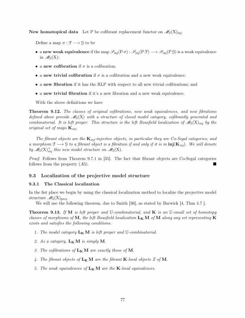
New homotopical data Let P be cofibrant replacement functor on MS(X)inj.

Define a map σ : F −→ G to be

• a new weak equivalence if the map Sinj(Pσ) : Sinj(PF) −→ Sinj(PG) is a weak equivalencein MS(X);

• a new cofibration if σ is a cofibration;

• a new trivial cofibration if σ is a cofibration and a new weak equivalence;

• a new fibration if it has the RLP with respect to all new trivial cofibrations; and

• a new trivial fibration if it’s a new fibration and a new weak equivalence.

With the above definitions we have

Theorem 9.12. The classes of original cofibrations, new weak equivalences, and new fibrationsdefined above provide MS(X) with a structure of closed model category, cofibrantly generated andcombinatorial. It is left proper. This structure is the left Bousfield localization of MS(X)inj by theoriginal set of maps Kinj.

The fibrant objects are the Kinj-injective objects, in particular they are Co-Segal categories; anda morphism F −→ G to a fibrant object is a fibration if and only if it is in inj(Kinj). We will denoteby MS(X)

+inj this new model structure on MS(X).

Proof. Follows from Theorem 9.7.1 in [35]. The fact that fibrant objects are Co-Segal categoriesfollows from the property (A5). �

9.3 Localization of the projective model structure

9.3.1 The Classical localization

In the fist place we begin by using the classical localization method to localize the projective modelstructure MS(X)proj.

We will use the following theorem, due to Smith [36], as stated by Barwick [4, Thm 4.7 ].

Theorem 9.13. If M is left proper and U-combinatorial, and K is an U-small set of homotopyclasses of morphisms of M, the left Bousfield localization LKM of M along any set representing K

exists and satisfies the following conditions.

1. The model category LKM is left proper and U-combinatorial.

2. As a category, LKM is simply M.

3. The cofibrations of LKM are exactly those of M.

4. The fibrant objects of LKM are the fibrant K-local objects Z of M.

5. The weak equivalences of LKM are the K-local equivalences.

77

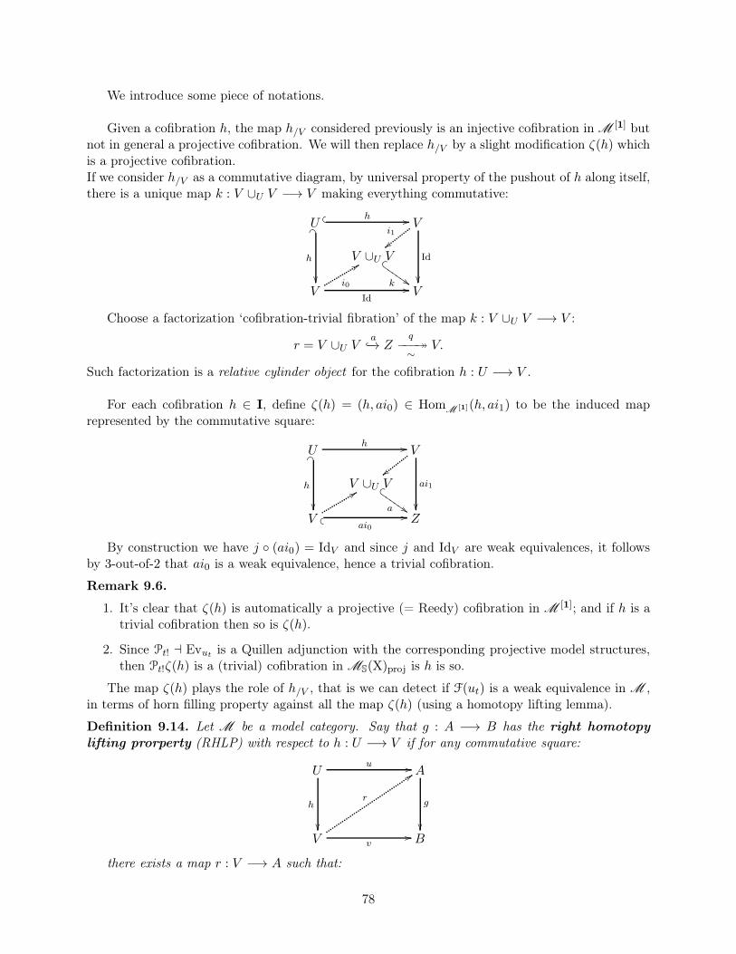
We introduce some piece of notations.

Given a cofibration h, the map h/V considered previously is an injective cofibration in M [1] butnot in general a projective cofibration. We will then replace h/V by a slight modification ζ(h) whichis a projective cofibration.If we consider h/V as a commutative diagram, by universal property of the pushout of h along itself,there is a unique map k : V ∪U V −→ V making everything commutative:

U V

V V

V ∪U V

� � h //_�

h

��

Id//

Id

��

i1

{{

i0

88 � r

k $$■■■■

■■

Choose a factorization ‘cofibration-trivial fibration’ of the map k : V ∪U V −→ V :

r = V ∪U Va−→ Z

q−−−։

∼V.

Such factorization is a relative cylinder object for the cofibration h : U −→ V .

For each cofibration h ∈ I, define ζ(h) = (h, ai0) ∈ HomM [1](h, ai1) to be the induced map

represented by the commutative square:

U V

V Z

V ∪U V

h //_�

h

����

ai0//

ai1

��

{{

88 � r

a $$■■■

■■■

By construction we have j ◦ (ai0) = IdV and since j and IdV are weak equivalences, it followsby 3-out-of-2 that ai0 is a weak equivalence, hence a trivial cofibration.

Remark 9.6.

1. It’s clear that ζ(h) is automatically a projective (= Reedy) cofibration in M [1]; and if h is atrivial cofibration then so is ζ(h).

2. Since Pt! ⊣ Evut is a Quillen adjunction with the corresponding projective model structures,then Pt!ζ(h) is a (trivial) cofibration in MS(X)proj is h is so.

The map ζ(h) plays the role of h/V , that is we can detect if F(ut) is a weak equivalence in M ,in terms of horn filling property against all the map ζ(h) (using a homotopy lifting lemma).

Definition 9.14. Let M be a model category. Say that g : A −→ B has the right homotopy

lifting prorperty (RHLP) with respect to h : U −→ V if for any commutative square:

U A

V B

u //

h

��

v//

g

��

r

::

there exists a map r : V −→ A such that:

78

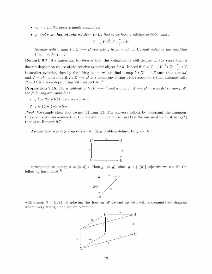
• rh = u i.e the upper triangle commutes;

• gr and v are homotopic relative to U , that is we have a relative cylinder object

V ∪U Va−→ Z

q−−−։

∼V

together with a map f : Z −→ B restricting to gu = vh on U ; and inducing the equalitiesfai0 = v, fai1 = gr.

Remark 9.7. It’s important to observe that this definition is well defined in the sense that it

doesn’t depend on choice of the relative cylinder object for h. Indeed if r′ = V ∪U Va′

−→ Z ′q′

−−−։∼

V

is another cylinder, then by the lifting axiom we can find a map k : Z ′ −→ Z such that a = ka′

and q′ = qk. Therefore if f : Z −→ B is a homotopy lifting with respect to r then automaticallyf ′ = fk is a homotopy lifting with respect to r′.

Proposition 9.15. For a cofibration h : U −→ V and a map g : A −→ B in a model category M ,the following are equivalent.

1. g has the RHLP with respect to h.

2. g is {ζ(h)}-injective.

Proof. We simply show how we get (1) from (2). The converse follows by ‘reversing’ the argumen-tation since we can assume that the relative cylinder chosen in (1) is the one used to construct ζ(h)thanks to Remark 9.7.

Assume that g is {ζ(h)}-injective. A lifting problem defined by g and h

U A

V B

u //

h

��

v//

g

��

corresponds to a map α = (u, v) ∈ HomM [1](h, g); since g is {ζ(h)}-injective we can fill the

following horn in M [1]

h g

ai1

α //

ζ(h)

��β

??

with a map β = (r, f). Displaying this horn in M we end up with with a commutative diagramwhere every triangle and square commute:

U A

V B

u //

h

��

g

��

v//

V

Z

ai1

��

h

yyrrrrrrrrrrrrrr

ai0

yyrrrrrrrrrrrrrr

r

33

f

33

79

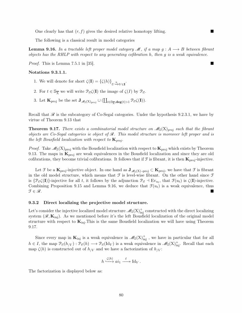
One clearly has that (r, f) gives the desired relative homotopy lifting. �

The following is a classical result in model categories

Lemma 9.16. In a tractable left proper model category M , if a map g : A −→ B between fibrantobjects has the RHLP with respect to any generating cofibration h, then g is a weak equivalence.

Proof. This is Lemma 7.5.1 in [35]. �

Notations 9.3.1.1.

1. We will denote for short ζ(I) = {ζ(h)}U

h−→V ∈I

.

2. For t ∈ SX we will write Pt!ζ(I) the image of ζ(I) by Pt!.

3. Let Kproj be the set JMS(X)proj∪ (

∐t∈SX,deg(t)>1 Pt!ζ(I)).

Recall that R is the subcategory of Co-Segal categories. Under the hypothesis 9.2.3.1, we have byvirtue of Theorem 9.13 that

Theorem 9.17. There exists a combinatorial model structure on MS(X)proj such that the fibrantobjects are Co-Segal categories ie object of R. This model structure is moreover left proper and isthe left Bousfield localization with respect to Kproj.

Proof. Take MS(X)proj with the Bousfield localization with respect to Kproj which exists by Theorem9.13. The maps in Kproj are weak equivalences in the Bousfield localization and since they are oldcofibrations, they become trivial cofibrations. It follows that if F is fibrant, it is then Kproj-injective.

Let F be a Kproj-injective object. In one hand as JMS(X) -proj ⊂ Kproj, we have that F is fibrantin the old model structure, which means that F is level-wise fibrant. On the other hand since F

is {Pt!ζ(I)}-injective for all t, it follows by the adjunction Pt! ⊣ Evut , that F(ut) is ζ(I)-injective.Combining Proposition 9.15 and Lemma 9.16, we deduce that F(ut) is a weak equivalence, thusF ∈ R. �

9.3.2 Direct localizing the projective model structure.

Let’s consider the injective localized model structure MS(X)+inj constructed with the direct localizing

system (R,Kinj). As we mentioned before it’s the left Bousfield localization of the original modelstructure with respect to Kinj.This is the same Bousfield localization we will have using Theorem9.17.

Since every map in Kinj is a weak equivalence in MS(X)+inj , we have in particular that for all

h ∈ I, the map Pt!(h/V ) : Pt!(h) −→ Pt!(IdV ) is a weak equivalence in MS(X)+inj. Recall that each

map ζ(h) is constructed out of h/V and we have a factorization of h/V :

hζ(h)−−→ ai1

ℓ−−։ IdV .

The factorization is displayed below as:

80

U V

V Z

V

V

h //_�

h

����

ai0//

_�

ai1≀

��

Id //

q∼ // //

Id

��

As q is a trivial fibration, ℓ : ai1 −→ Id is a level-wise trivial fibration in M [1] in particulara weak equivalence therein. Since we’ve assumed that all the objects of M are cofibrant, thenboth the source and target of ℓ are cofibrant in M 2

proj. From Ken Brown lemma Pt! preservesweak equivalences between cofibrant objects (as any left Quillen functor); thus Pt!(ℓ) is an old weakequivalence, hence a new weak equivalence (= a weak equivalence in MS(X)

+inj).

From the equality Pt!(h/V ) = Pt!(ℓ)◦Pt!ζ(h) we deduce by 3 for 2 in the model category MS(X)+inj,

that Pt!ζ(h) is a weak equivalence therein; moreover since projective cofibrations are also injectivecofibration, then Pt!ζ(h) is an old cofibration, hence a new cofibration. Putting these together onehas that every Pt!ζ(h) is a trivial cofibration in MS(X)

+inj.

New projective data Recall that weak equivalences in MS(X)+inj are those maps σ such that

Sinj(Pσ) is a weak equivalence in the original model structure MS(X)inj. Here Sinj is a weakmonadic projection from MS(X)inj to R and P is a cofibrant replacement functor in MS(X)inj. Aspointed out in [35, Sec 9.3], the notion of new weak equivalence depends only on R and doesn’tdepend neither on Kinj nor on P.

Using again the fact that projective cofibrations are injective ones, and since old weak equiva-lences in MS(X)inj and MS(X)proj are the same, we clearly have that a cofibrant replacement functorin MS(X)proj is also a cofibrant replacement for MS(X)inj. Therefore we can assume that P is aprojective cofibrant replacement functor.

As mentioned in the Remark 9.3 we can extract from the weak monadic projection Sinj aweak monadic projection Sproj from MS(X)proj to R. This is obtained by applying the functorialfactorization of the type (cof ,fib∩we) to the natural transformation η : IdMS(X) −→ Sinj in themodel category MS(X)proj. In particular there is trivial projective fibration Sproj −→ Sinj.

Warning. In the upcoming paragraphs we will precise ‘new injective’ or ‘new projective’ to avoidconfusion when saying ‘new weak equivalence’. We will remove this disctinction later since the newweak equivalences will be the same.

Let P be cofibrant replacement functor on MS(X)proj.

Define a map σ : F −→ G to be:

• a new projective weak equivalence if the map Sproj(Pσ) : Sproj(PF) −→ Sproj(PG) isa weak equivalence in MS(X) ;

• a new cofibration if σ is a cofibration;

• a new trivial cofibration if σ is a cofibration and a new (projective) weak equivalence;

81

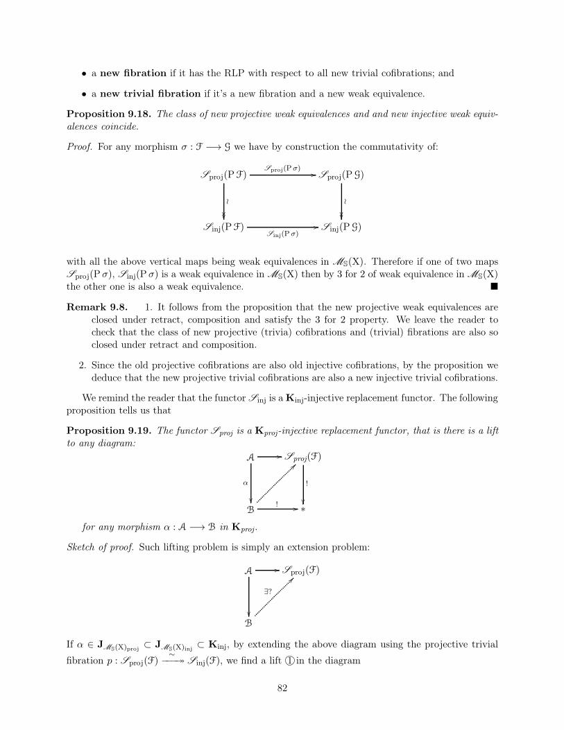
• a new fibration if it has the RLP with respect to all new trivial cofibrations; and

• a new trivial fibration if it’s a new fibration and a new weak equivalence.

Proposition 9.18. The class of new projective weak equivalences and and new injective weak equiv-alences coincide.

Proof. For any morphism σ : F −→ G we have by construction the commutativity of:

Sproj(PF) Sproj(PG)

Sinj(PF) Sinj(PG)

Sproj(Pσ) //

≀

����

Sinj(Pσ)//

≀

����

with all the above vertical maps being weak equivalences in MS(X). Therefore if one of two mapsSproj(Pσ), Sinj(Pσ) is a weak equivalence in MS(X) then by 3 for 2 of weak equivalence in MS(X)the other one is also a weak equivalence. �

Remark 9.8. 1. It follows from the proposition that the new projective weak equivalences areclosed under retract, composition and satisfy the 3 for 2 property. We leave the reader tocheck that the class of new projective (trivia) cofibrations and (trivial) fibrations are also soclosed under retract and composition.

2. Since the old projective cofibrations are also old injective cofibrations, by the proposition wededuce that the new projective trivial cofibrations are also a new injective trivial cofibrations.

We remind the reader that the functor Sinj is a Kinj-injective replacement functor. The followingproposition tells us that

Proposition 9.19. The functor Sproj is a Kproj-injective replacement functor, that is there is a liftto any diagram:

A Sproj(F)

B ∗

//

α

��

!

��! //

??

for any morphism α : A −→ B in Kproj.

Sketch of proof. Such lifting problem is simply an extension problem:

A Sproj(F)

B

//

��

∃?

??

If α ∈ JMS(X)proj⊂ JMS(X)inj

⊂ Kinj, by extending the above diagram using the projective trivial

fibration p : Sproj(F)∼−−−։ Sinj(F), we find a lift 1 in the diagram

82

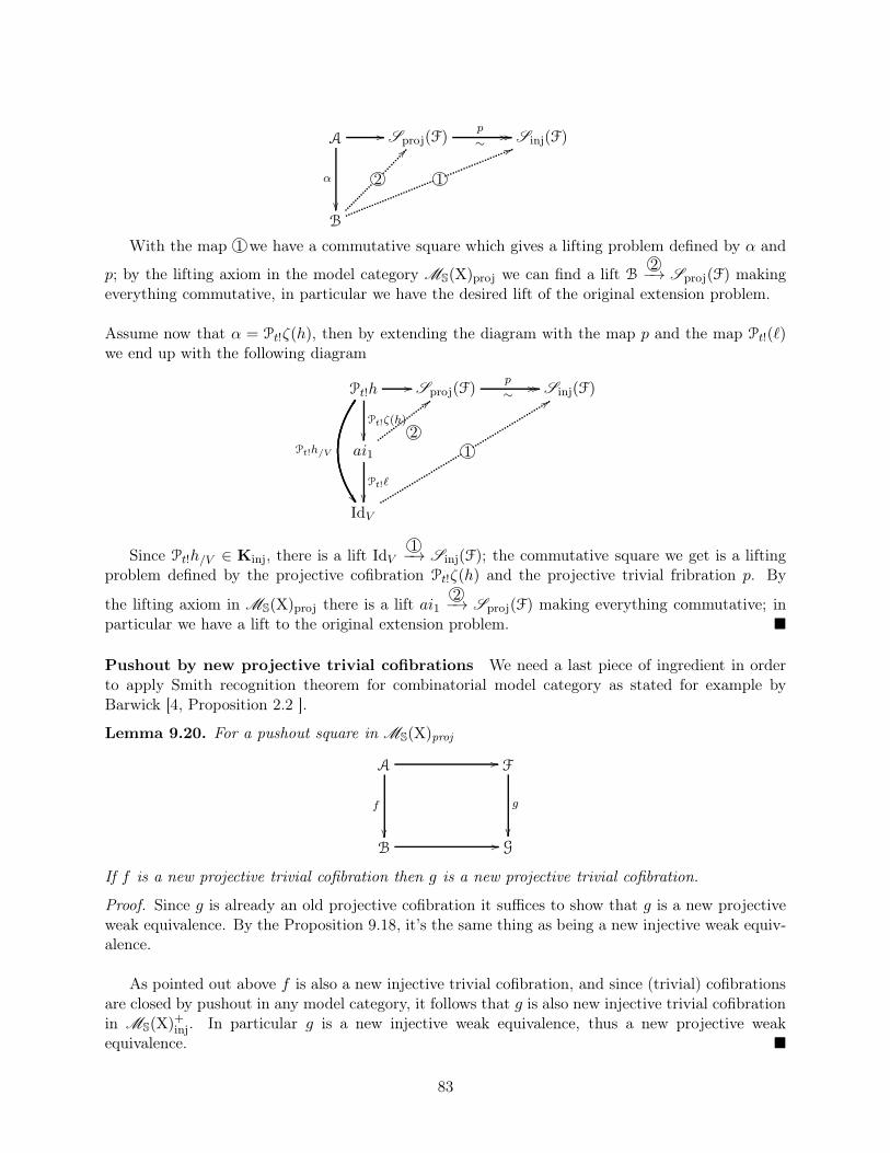
A Sproj(F)

B

Sinj(F)//

α

��

p

∼// //

1

55

2

??

With the map 1 we have a commutative square which gives a lifting problem defined by α and

p; by the lifting axiom in the model category MS(X)proj we can find a lift B2−→ Sproj(F) making

everything commutative, in particular we have the desired lift of the original extension problem.

Assume now that α = Pt!ζ(h), then by extending the diagram with the map p and the map Pt!(ℓ)we end up with the following diagram

Pt!h Sproj(F)

ai1

Sinj(F)

IdV

//

Pt!ζ(h)

��

p

∼// //

Pt!ℓ

��

1

99

Pt!h/V

��

2

;;

Since Pt!h/V ∈ Kinj, there is a lift IdV1−→ Sinj(F); the commutative square we get is a lifting

problem defined by the projective cofibration Pt!ζ(h) and the projective trivial fribration p. By

the lifting axiom in MS(X)proj there is a lift ai12−→ Sproj(F) making everything commutative; in

particular we have a lift to the original extension problem. �

Pushout by new projective trivial cofibrations We need a last piece of ingredient in orderto apply Smith recognition theorem for combinatorial model category as stated for example byBarwick [4, Proposition 2.2 ].

Lemma 9.20. For a pushout square in MS(X)proj

A F

B G

//

f

��//

g

��

If f is a new projective trivial cofibration then g is a new projective trivial cofibration.

Proof. Since g is already an old projective cofibration it suffices to show that g is a new projectiveweak equivalence. By the Proposition 9.18, it’s the same thing as being a new injective weak equiv-alence.

As pointed out above f is also a new injective trivial cofibration, and since (trivial) cofibrationsare closed by pushout in any model category, it follows that g is also new injective trivial cofibrationin MS(X)

+inj. In particular g is a new injective weak equivalence, thus a new projective weak

equivalence. �

83

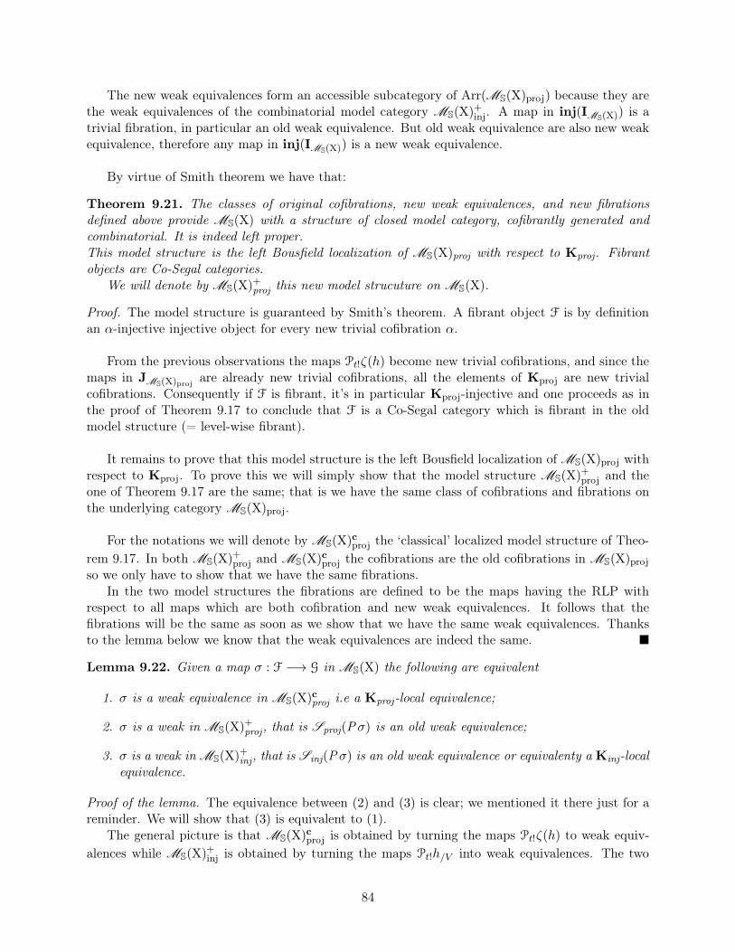
The new weak equivalences form an accessible subcategory of Arr(MS(X)proj) because they arethe weak equivalences of the combinatorial model category MS(X)

+inj. A map in inj(IMS(X)) is a

trivial fibration, in particular an old weak equivalence. But old weak equivalence are also new weakequivalence, therefore any map in inj(IMS(X)) is a new weak equivalence.

By virtue of Smith theorem we have that:

Theorem 9.21. The classes of original cofibrations, new weak equivalences, and new fibrationsdefined above provide MS(X) with a structure of closed model category, cofibrantly generated andcombinatorial. It is indeed left proper.This model structure is the left Bousfield localization of MS(X)proj with respect to Kproj. Fibrantobjects are Co-Segal categories.

We will denote by MS(X)+proj this new model strucuture on MS(X).

Proof. The model structure is guaranteed by Smith’s theorem. A fibrant object F is by definitionan α-injective injective object for every new trivial cofibration α.

From the previous observations the maps Pt!ζ(h) become new trivial cofibrations, and since themaps in JMS(X)proj

are already new trivial cofibrations, all the elements of Kproj are new trivialcofibrations. Consequently if F is fibrant, it’s in particular Kproj-injective and one proceeds as inthe proof of Theorem 9.17 to conclude that F is a Co-Segal category which is fibrant in the oldmodel structure (= level-wise fibrant).

It remains to prove that this model structure is the left Bousfield localization of MS(X)proj withrespect to Kproj. To prove this we will simply show that the model structure MS(X)

+proj and the

one of Theorem 9.17 are the same; that is we have the same class of cofibrations and fibrations onthe underlying category MS(X)proj.

For the notations we will denote by MS(X)cproj the ‘classical’ localized model structure of Theo-

rem 9.17. In both MS(X)+proj and MS(X)

cproj the cofibrations are the old cofibrations in MS(X)proj

so we only have to show that we have the same fibrations.In the two model structures the fibrations are defined to be the maps having the RLP with

respect to all maps which are both cofibration and new weak equivalences. It follows that thefibrations will be the same as soon as we show that we have the same weak equivalences. Thanksto the lemma below we know that the weak equivalences are indeed the same. �

Lemma 9.22. Given a map σ : F −→ G in MS(X) the following are equivalent

1. σ is a weak equivalence in MS(X)cproj i.e a Kproj-local equivalence;

2. σ is a weak in MS(X)+proj, that is Sproj(P σ) is an old weak equivalence;

3. σ is a weak in MS(X)+inj, that is Sinj(P σ) is an old weak equivalence or equivalenty a Kinj-local

equivalence.

Proof of the lemma. The equivalence between (2) and (3) is clear; we mentioned it there just for areminder. We will show that (3) is equivalent to (1).

The general picture is that MS(X)cproj is obtained by turning the maps Pt!ζ(h) to weak equiv-

alences while MS(X)+inj is obtained by turning the maps Pt!h/V into weak equivalences. The two

84

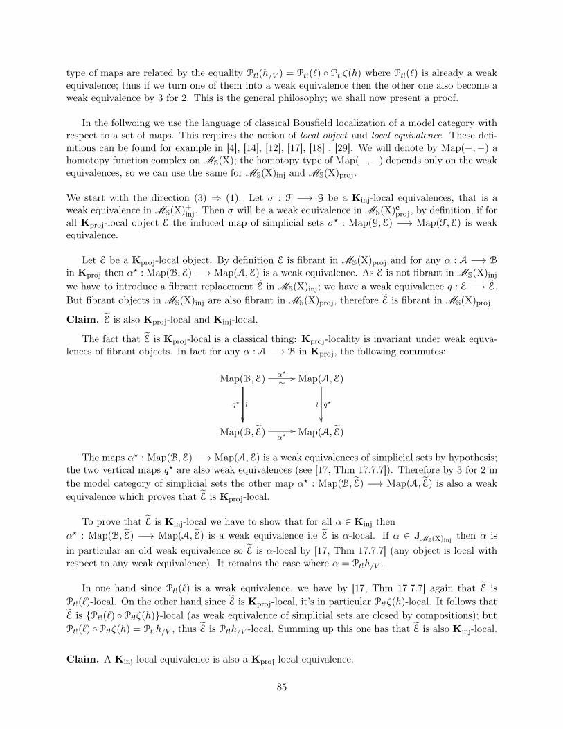
type of maps are related by the equality Pt!(h/V ) = Pt!(ℓ) ◦ Pt!ζ(h) where Pt!(ℓ) is already a weakequivalence; thus if we turn one of them into a weak equivalence then the other one also become aweak equivalence by 3 for 2. This is the general philosophy; we shall now present a proof.

In the follwoing we use the language of classical Bousfield localization of a model category withrespect to a set of maps. This requires the notion of local object and local equivalence. These defi-nitions can be found for example in [4], [14], [12], [17], [18] , [29]. We will denote by Map(−,−) ahomotopy function complex on MS(X); the homotopy type of Map(−,−) depends only on the weakequivalences, so we can use the same for MS(X)inj and MS(X)proj.

We start with the direction (3) ⇒ (1). Let σ : F −→ G be a Kinj-local equivalences, that is aweak equivalence in MS(X)

+inj. Then σ will be a weak equivalence in MS(X)

cproj, by definition, if for

all Kproj-local object E the induced map of simplicial sets σ⋆ : Map(G,E) −→ Map(F,E) is weakequivalence.

Let E be a Kproj-local object. By definition E is fibrant in MS(X)proj and for any α : A −→ B

in Kproj then α⋆ : Map(B,E) −→ Map(A,E) is a weak equivalence. As E is not fibrant in MS(X)inj

we have to introduce a fibrant replacement E in MS(X)inj; we have a weak equivalence q : E −→ E.

But fibrant objects in MS(X)inj are also fibrant in MS(X)proj, therefore E is fibrant in MS(X)proj.

Claim. E is also Kproj-local and Kinj-local.

The fact that E is Kproj-local is a classical thing: Kproj-locality is invariant under weak equva-lences of fibrant objects. In fact for any α : A −→ B in Kproj, the following commutes:

Map(B,E) Map(A,E)

Map(B, E) Map(A, E)

α⋆

∼//

q⋆ ≀

��

α⋆//

q⋆≀

��

The maps α⋆ : Map(B,E) −→ Map(A,E) is a weak equivalences of simplicial sets by hypothesis;the two vertical maps q⋆ are also weak equivalences (see [17, Thm 17.7.7]). Therefore by 3 for 2 in

the model category of simplicial sets the other map α⋆ : Map(B, E) −→ Map(A, E) is also a weak

equivalence which proves that E is Kproj-local.

To prove that E is Kinj-local we have to show that for all α ∈ Kinj then

α⋆ : Map(B, E) −→ Map(A, E) is a weak equivalence i.e E is α-local. If α ∈ JMS(X)injthen α is

in particular an old weak equivalence so E is α-local by [17, Thm 17.7.7] (any object is local withrespect to any weak equivalence). It remains the case where α = Pt!h/V .

In one hand since Pt!(ℓ) is a weak equivalence, we have by [17, Thm 17.7.7] again that E is

Pt!(ℓ)-local. On the other hand since E is Kproj-local, it’s in particular Pt!ζ(h)-local. It follows that

E is {Pt!(ℓ) ◦ Pt!ζ(h)}-local (as weak equivalence of simplicial sets are closed by compositions); but

Pt!(ℓ) ◦Pt!ζ(h) = Pt!h/V , thus E is Pt!h/V -local. Summing up this one has that E is also Kinj-local.

Claim. A Kinj-local equivalence is also a Kproj-local equivalence.

85

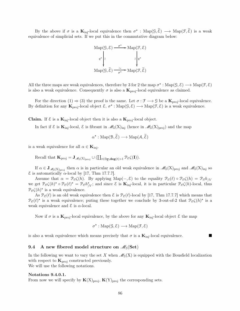
By the above if σ is a Kinj-local equivalence then σ⋆ : Map(G, E) −→ Map(F, E) is a weakequivalence of simplicial sets. If we put this in the commutative diagram below:

Map(G,E) Map(F,E)

Map(G, E) Map(F, E)

σ⋆ //

q⋆ ≀

��

σ⋆∼ //

q⋆≀

��

All the three maps are weak equivalences, therefore by 3 for 2 the map σ⋆ : Map(G,E) −→ Map(F,E)is also a weak equivalence. Consequently σ is also a Kproj-local equivalence as claimed.

For the direction (1)⇒ (3) the proof is the same. Let σ : F −→ G be a Kproj-local equivalence.By definition for any Kproj-local object E, σ⋆ : Map(G,E) −→ Map(F,E) is a weak equivalence.

Claim. If E is a Kinj-local object then it is also a Kproj-local object.

In fact if E is Kinj-local, E is fibrant in MS(X)inj (hence in MS(X)proj) and the map

α⋆ : Map(B, E) −→ Map(A, E)

is a weak equivalence for all α ∈ Kinj.

Recall that Kproj = JMS(X)proj∪ (

∐t∈SX,deg(t)>1 Pt!ζ(I)).

If α ∈ JMS(X)projthen α is in particular an old weak equivalence in MS(X)proj and MS(X)inj so

E is automatically α-local by [17, Thm 17.7.7].Assume that α = Pt!ζ(h). By applying Map(−,E) to the equality Pt!(ℓ) ◦ Pt!ζ(h) = Pt!h/V

we get Pt!ζ(h)⋆ ◦ Pt!(ℓ)

⋆ = Pt!h⋆/V ; and since E is Kinj-local, it is in particular Pt!ζ(h)-local, thus

Pt!ζ(h)⋆ is a weak equivalence.

As Pt!(ℓ) is an old weak equivalence then E is Pt!(ℓ)-local by [17, Thm 17.7.7] which means thatPt!(ℓ)

⋆ is a weak equivalence; puting these together we conclude by 3-out-of-2 that Pt!ζ(h)⋆ is a

weak equivalence and E is α-local.

Now if σ is a Kproj-local equivalence, by the above for any Kinj-local object E the map

σ⋆ : Map(G,E) −→ Map(F,E)

is also a weak equivalence which means precisely that σ is a Kinj-local equivalence. �

9.4 A new fibered model structure on MS(Set)

In the following we want to vary the set X when MS(X) is equipped with the Bousfield localizationwith respect to Kproj constructed previously.We will use the following notations.

Notations 9.4.0.1.From now we will specify by K(X)proj, K(Y)proj the corresponding sets.

86

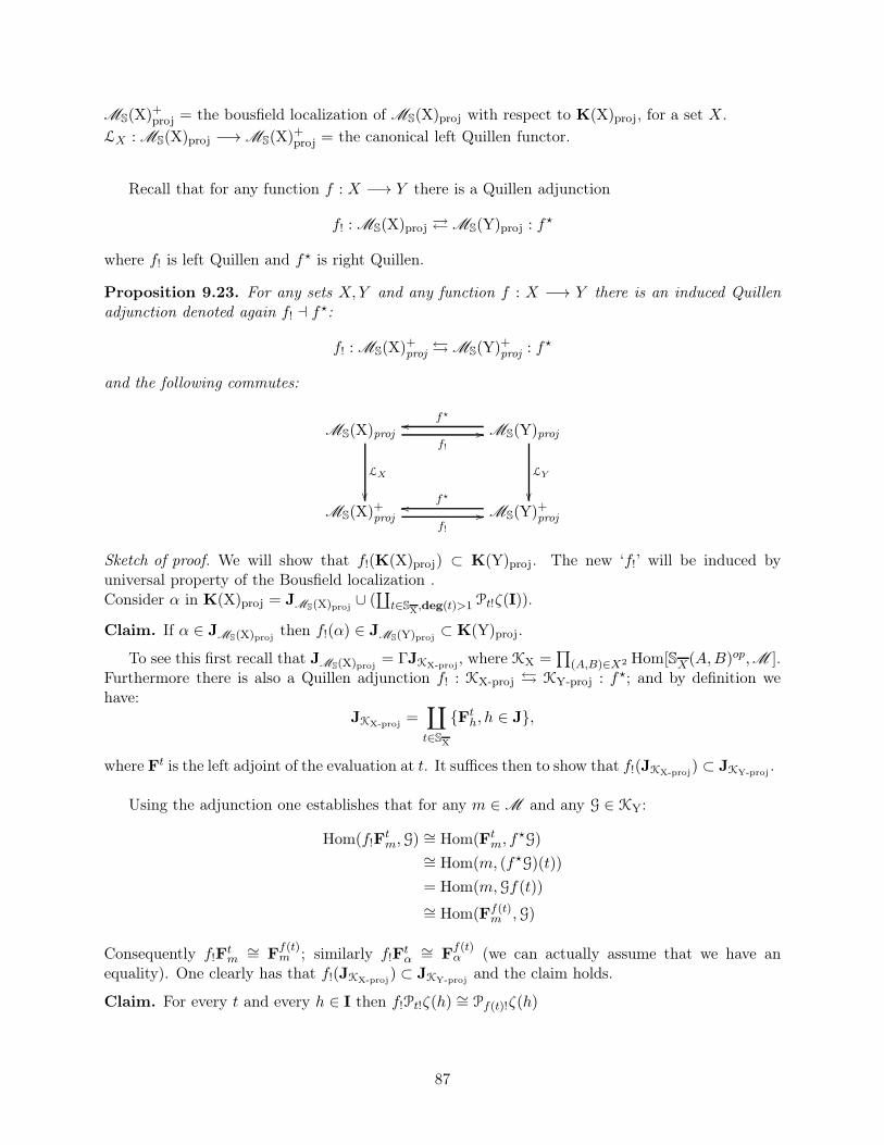
MS(X)+proj = the bousfield localization of MS(X)proj with respect to K(X)proj, for a set X.

LX : MS(X)proj −→MS(X)+proj = the canonical left Quillen functor.

Recall that for any function f : X −→ Y there is a Quillen adjunction

f! : MS(X)proj ⇄MS(Y)proj : f⋆

where f! is left Quillen and f⋆ is right Quillen.

Proposition 9.23. For any sets X,Y and any function f : X −→ Y there is an induced Quillenadjunction denoted again f! ⊣ f

⋆:

f! : MS(X)+proj ⇆MS(Y)

+proj : f

⋆

and the following commutes:

MS(X)proj MS(Y)proj

MS(X)+proj MS(Y)

+proj

f!//

oo f⋆

LX

��

LY

��

f!//

oo f⋆

Sketch of proof. We will show that f!(K(X)proj) ⊂ K(Y)proj. The new ‘f!’ will be induced byuniversal property of the Bousfield localization .Consider α in K(X)proj = JMS(X)proj

∪ (∐t∈SX,deg(t)>1 Pt!ζ(I)).

Claim. If α ∈ JMS(X)projthen f!(α) ∈ JMS(Y)proj

⊂ K(Y)proj.

To see this first recall that JMS(X)proj= ΓJKX-proj

, where KX =∏

(A,B)∈X2 Hom[SX(A,B)op,M ].Furthermore there is also a Quillen adjunction f! : KX-proj ⇆ KY-proj : f

⋆; and by definition wehave:

JKX-proj=

∐

t∈SX

{Fth, h ∈ J},

where Ft is the left adjoint of the evaluation at t. It suffices then to show that f!(JKX-proj) ⊂ JKY-proj

.

Using the adjunction one establishes that for any m ∈M and any G ∈ KY:

Hom(f!Ftm,G)

∼= Hom(Ftm, f⋆G)

∼= Hom(m, (f⋆G)(t))

= Hom(m,Gf(t))

∼= Hom(Ff(t)m ,G)

Consequently f!Ftm∼= F

f(t)m ; similarly f!F

tα∼= F

f(t)α (we can actually assume that we have an

equality). One clearly has that f!(JKX-proj) ⊂ JKY-proj

and the claim holds.

Claim. For every t and every h ∈ I then f!Pt!ζ(h) ∼= Pf(t)!ζ(h)

87

This also holds by the adjunction. For any h and any G ∈MS(Y) one has:

Hom(f!Pt!ζ(h),G) ∼= Hom(Pt!ζ(h), f⋆G)

∼= Hom(ζ(h), (f⋆G)(ut))

= Hom(ζ(h),G f(ut)︸ ︷︷ ︸=uf(t)

)

= Hom(ζ(h),Guf(t))

∼= Hom(Pf(t)!ζ(h),G)

and the claim follows. If we combine the two claims we have the desired result �

By virtue of Roig-Stanculescu result (Theorem 8.7) and under the hypothesis (9.2.3.1) we have

Theorem 9.24. For a symmetric closed monoidal model category M whose objects are all cofibrant,the category MS(Set) has a Quillen model structure where a map σ = (f, σ) : F −→ G is

1. a weak equivalence if f : X −→ Y is an isomorphism of sets and σ : F −→ f⋆G is a weakequivalence in MS(X)

+proj,

2. a cofibration if the adjoint map σ : f!F −→ G is a cofibration in MS(Y)+proj,

3. a fibration if σ : F −→ f⋆G is a fibration in MS(X)+proj.

4. fibrant objects are Co-Segal categories

We will denote by MS(Set)+proj the new model structure on MS(Set). There is a canonical leftQuillen functor

L : MS(Set)proj −→MS(Set)+proj

whose component over X is LX : MS(X)proj −→MS(X)+proj.

Proof. The proof is the same as for Theorem ??. On Set we take the minimal model structure:cofibrations and fibrations are all maps, weak equivalences are isomorphisms. One can check eas-ily that all the conditions of Theorem 8.7 are fulfilled; this gives the model structure described above.

For F ∈ MS(X)+proj, F is fibrant if the canonical map : F −→ ∗ is a fibration MS(Set)+proj,

where ∗ is the terminal object therein. By definition this is equivalent to have that : F −→ ⋆∗is fibration is MS(X)

+proj; and since ⋆ is a right adjoint then it preserves the terminal object (as it

preserves any limit).

Summing up this one has that F is fibrant in MS(Set)+proj if and only if it is fibrant in MS(X)+proj,

therefore F is a Co-segal category by Theorem 9.21. �

9.4.1 Cofibrantly generated

Since the cofibrations on MS(Set)proj and MS(Set)+proj are the same, the set IMS(Set)projconstitutes

also a generating set for the cofibrations in MS(Set)+proj. Using the fact that MS(Set)+proj is alreadya model category which is locally presentable, one can easily check that the set IMS(Set)proj

and the

class of weak equivalences of MS(Set)+proj satisfy the conditions Smith’s recognition theorem ([4,

88

Proposition 2.2]).

By Smith’s theorem we have a combinatorial model structure on MS(Set)proj with the same

cofibrations and weak equivalences of MS(Set)+proj. The set IMS(Set)projconstitutes a generating set

for the cofibrations and there exists a set JMS(Set)+

projwhich is a set of generating trivial cofibrations.

But since this new model category has the same cofibrations and weak equivalences (hence thesame fibrations) as MS(Set)+proj we deduce that this new model structure is in fact isomorphic to

MS(Set)proj; thus MS(Set)+proj is combinatorial and in particular cofibrantly generated.

89

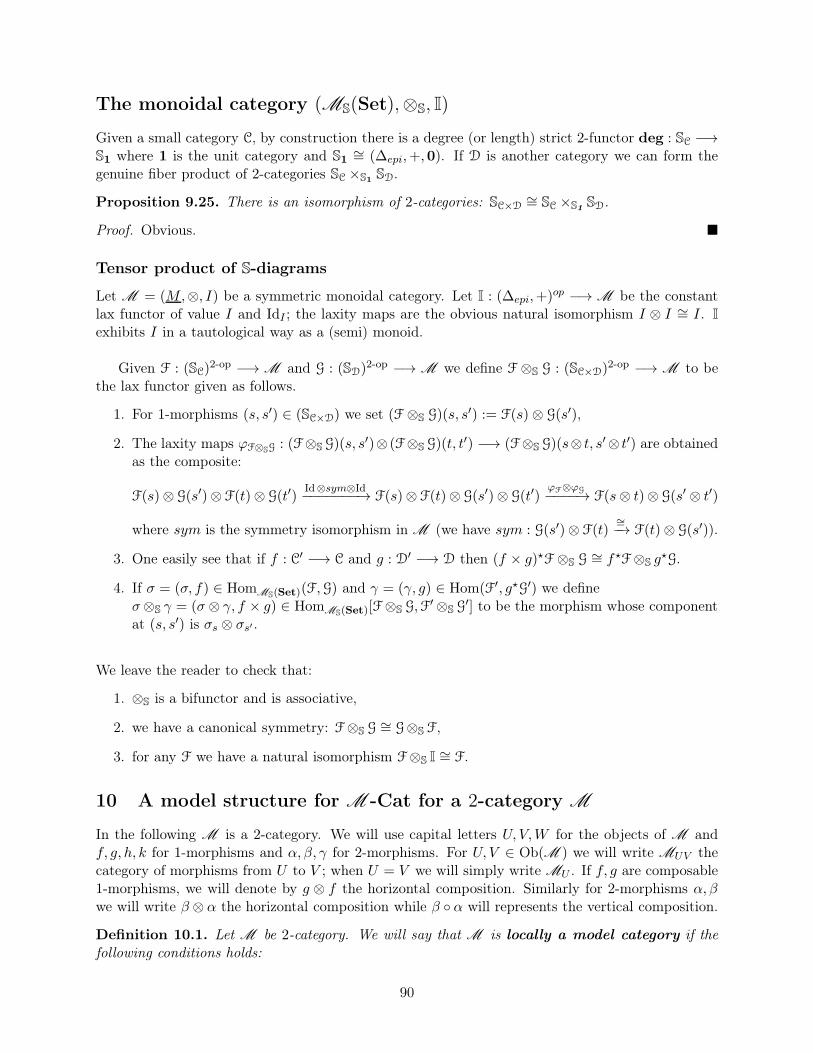
The monoidal category (MS(Set),⊗S, I)

Given a small category C, by construction there is a degree (or length) strict 2-functor deg : SC −→S1 where 1 is the unit category and S1

∼= (∆epi,+,0). If D is another category we can form thegenuine fiber product of 2-categories SC ×S1 SD.

Proposition 9.25. There is an isomorphism of 2-categories: SC×D∼= SC ×S1 SD.

Proof. Obvious. �

Tensor product of S-diagrams

Let M = (M,⊗, I) be a symmetric monoidal category. Let I : (∆epi,+)op −→M be the constantlax functor of value I and IdI ; the laxity maps are the obvious natural isomorphism I ⊗ I ∼= I. I

exhibits I in a tautological way as a (semi) monoid.

Given F : (SC)2-op −→M and G : (SD)

2-op −→M we define F ⊗S G : (SC×D)2-op −→M to be

the lax functor given as follows.

1. For 1-morphisms (s, s′) ∈ (SC×D) we set (F ⊗S G)(s, s′) := F(s)⊗ G(s′),

2. The laxity maps ϕF⊗SG : (F⊗SG)(s, s′)⊗ (F⊗S G)(t, t

′) −→ (F⊗S G)(s⊗ t, s′⊗ t′) are obtained

as the composite:

F(s)⊗ G(s′)⊗ F(t)⊗ G(t′)Id⊗sym⊗Id−−−−−−−→ F(s)⊗ F(t)⊗ G(s′)⊗ G(t′)

ϕF⊗ϕG−−−−→ F(s⊗ t)⊗ G(s′ ⊗ t′)

where sym is the symmetry isomorphism in M (we have sym : G(s′)⊗ F(t)∼=−→ F(t)⊗ G(s′)).

3. One easily see that if f : C′ −→ C and g : D′ −→ D then (f × g)⋆F ⊗S G∼= f⋆F⊗S g

⋆G.

4. If σ = (σ, f) ∈ HomMS(Set)(F,G) and γ = (γ, g) ∈ Hom(F′, g⋆G′) we defineσ⊗S γ = (σ ⊗ γ, f × g) ∈ HomMS(Set)[F⊗S G,F

′⊗S G′] to be the morphism whose component

at (s, s′) is σs ⊗ σs′ .

We leave the reader to check that:

1. ⊗S is a bifunctor and is associative,

2. we have a canonical symmetry: F⊗S G∼= G⊗S F,

3. for any F we have a natural isomorphism F⊗S I ∼= F.

10 A model structure for M -Cat for a 2-category M

In the following M is a 2-category. We will use capital letters U, V,W for the objects of M andf, g, h, k for 1-morphisms and α, β, γ for 2-morphisms. For U, V ∈ Ob(M ) we will write MUV thecategory of morphisms from U to V ; when U = V we will simply write MU . If f, g are composable1-morphisms, we will denote by g ⊗ f the horizontal composition. Similarly for 2-morphisms α, βwe will write β ⊗ α the horizontal composition while β ◦ α will represents the vertical composition.

Definition 10.1. Let M be 2-category. We will say that M is locally a model category if thefollowing conditions holds:

90

1. Each MUV is a model category in the usual sense.

2. M is a biclosed that is: for every 1-morphism f the following functors have a right adjoint:

f ⊗− −⊗f

3. The pushout-product axiom holds: given two cofibrations α : f −→ g ∈ Arr(MUV ) andβ : k −→ h ∈ Arr(MV W ) then the induced map β�α : h ⊗ f ∪k⊗f k ⊗ g −→ h ⊗ g is acofibration in MUW which is moreover a trivial cofibration if either α or β is .

4. For every U and any 1-morphism f ∈ MUV , if Q(IdU ) −→ IdU is a cofibrant replacementthen the induced map Q(IdU )⊗ f −→ f is a weak equivalence in MUV .

As one can see this is a straightforward generalization of a monoidal model category consideredas a 2-category with one object. The condition (2) allows to distribute colimits with respect to thecomposition on each factor.

We recall briefly below the definition of a category enriched over a 2-category M .

An M -category X consists roughly speaking of:

1. for each object U of M , a set XU of objects over U ;

2. for objects A,B over U, V , respectively an arrow X (A,B) : U −→ V ∈MUV ;

3. for each object A over U , a 2-cell IA : IdU =⇒X (A,A) ∈MU ;

4. for object A,B,C over U, V,W , respectively, a 2-cell cABC : X (B,C) ⊗ X (A,B) =⇒X (A,C) ∈ MUW satisfying the obvious three axioms of left and right identities and as-sociativity.

Equivalently X can be defined as a lax morphism X : X −→ M or a strict homomorphismX : PX −→ M (see [3]). Note that for each U , we have a category X|U enriched over themonoidal category MU ; the set of objects of X|U is XU .

Given two M -categories X and Y an M -functor is given the following data:

1. a function Φ : Ob(X ) −→ Ob(Y ), Φ =∐U ΦU with ΦU : XU −→ YU ;

2. for A,B in X over U, V , respectively we have a morphism ΦAB : X (A,B) −→ Y (ΦA,ΦB)in MUV

3. for each object A over U we have IΦA = ΦAA ◦ IA; satisfying the obvious compatibility withrespect to the composition on both sides.

M -categories with M -functors form the category M -Cat. There is an obvious category M -Graph whose objects are M -graphs and morphisms are just the natural ones.

We have a forgetful functor just like in the monoidal case U : M -Cat −→M -Graph.

Remark 10.1. As usual there is a restriction Φ|U : X|U −→ Y|U of Φ, which is a MU -functor. Andany M -functor has an underlying morphism between the corresponding M -graphs.

91

Proposition 10.2. Let M be a biclosed 2-category which is locally locally-presentable that is:each MUV is locally presentable in the usual sense. Then M -Cat is locally presentable.

Proof. All is proved in the same manner as for a monoidal category M . Below we list the differentsteps:

1. First one shows that M -Graph is cocomplete, this is easy, just apply the same method asWolff [39]

2. U is monadic: construct a left adjoint of U with the same formula given in [39]. Then showthat M -Cat has coequalizer of parallel U-split pair, again using the same idea in loc. cit. AsU clearly reflect isomorphisms, it follows by Beck monadicity theorem that U is monadic.

3. Linton’s result [28, Corollary 2] applies and one has that M -Cat is cocomplete as well.

4. Following the same method as Kelly and Lack [21] one has that the monad induced by U

preserves filtered colimits and M -Graph is locally presentable. From this we apply [1, Remark2.78] to establish that M -Cat is also locally presentable.

Note that being biclosed is essential in order to permute (filtered) colimits and ⊗. �

Terminology. Let W be a class of 2-morphisms in M . An M -functor Φ : X −→ Y is said to belocally in W if for every pair of objects A,B of X the 2-morphism ΦAB : X (A,B) −→ Y (ΦA,ΦB)is in W . We will say the same thing for a morphism between M -graphs.

The category M -Cat(X)

For each U ∈ M let’s fix a set XU of objects over U and consider X =∐U XU . Denote by

M -Cat(X) the category of M -categories with fixed set of objects X and M -functors which fixe X.Similarly there is a category M -Graph(X) of M -graphs with vertices X and morphisms fixing X.

Just like in the case where M is a monoidal category there is a tensor product in M -Graph(X)defined as follows. If X ,Y ∈M -Graph(X) one defines X ⊗X Y by:

(X ⊗X Y )(A,B) =∐

Z∈X

X (A,Z)⊗ Y (Z,B).

The unity of this product is the M -graph I given by

I (A,B) =

{IdU if A and B are over the same object U

∅ = initial object in MUV If A over U , and B over V with U 6= V

As usual it’s not hard to see that M -Cat(X) is the category of monoids of (M -Graph(X),⊗X ,I ).We have an obvious isomorphism of categories:

M -Graph(X) ∼=∏

(U,V )∈Ob(M )2

M(XU×XV )UV

where M(XU×XV )UV = Hom(XU × XV ,MUV ). From this we can endow M -Graph(X) with the

product model structure. In this model structure, fibrations, cofibrations and weak equivalences aresimply component wise such morphism.

92

Theorem 10.3. Let M be a 2-category which is locally a model category and locally cofibrantlygenerated. Assume moreover that all the objects of M are cofibrant. Then we have:

1. the category M -Cat(X) admits a model structure which is cofibrantly generated.

2. if M is combinatorial, then so is M -Cat(X)

Proof. This is a special case of theorem 3.12 where O = OX , C. = X and M. = M �

Remark 10.2. One can remove the hypothesis ‘all the objects of M are cofibrant’ by using ananalogue of the monoid axiom of [34]. In fact one can use the method in loc. cit to establish thetheorem. Lurie [29] also presented a nice description of the model structure for the case where M isthe monoidal category of simplicial sets. It seems obvious that we can adapt his method to calculatethe pushout of interest in our case.

93

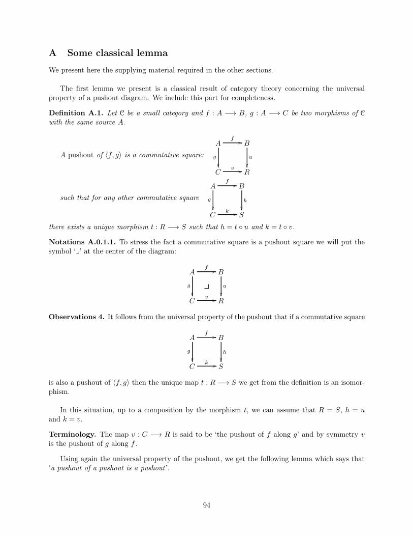
A Some classical lemma

We present here the supplying material required in the other sections.

The first lemma we present is a classical result of category theory concerning the universalproperty of a pushout diagram. We include this part for completeness.

Definition A.1. Let C be a small category and f : A −→ B, g : A −→ C be two morphisms of Cwith the same source A.

A pushout of 〈f, g〉 is a commutative square:

A B

C R

f //

g

��u

��v //

such that for any other commutative square

A B

C S

f //

g

��h

��k //

there exists a unique morphism t : R −→ S such that h = t ◦ u and k = t ◦ v.

Notations A.0.1.1. To stress the fact a commutative square is a pushout square we will put thesymbol ‘y’ at the center of the diagram:

A B

C R

y

f //

g

��u

��v //

Observations 4. It follows from the universal property of the pushout that if a commutative square

A B

C S

f //

g

��h

��k //

is also a pushout of 〈f, g〉 then the unique map t : R −→ S we get from the definition is an isomor-phism.

In this situation, up to a composition by the morphism t, we can assume that R = S, h = uand k = v.

Terminology. The map v : C −→ R is said to be ‘the pushout of f along g’ and by symmetry vis the pushout of g along f .

Using again the universal property of the pushout, we get the following lemma which says that‘a pushout of a pushout is a pushout ’.

94

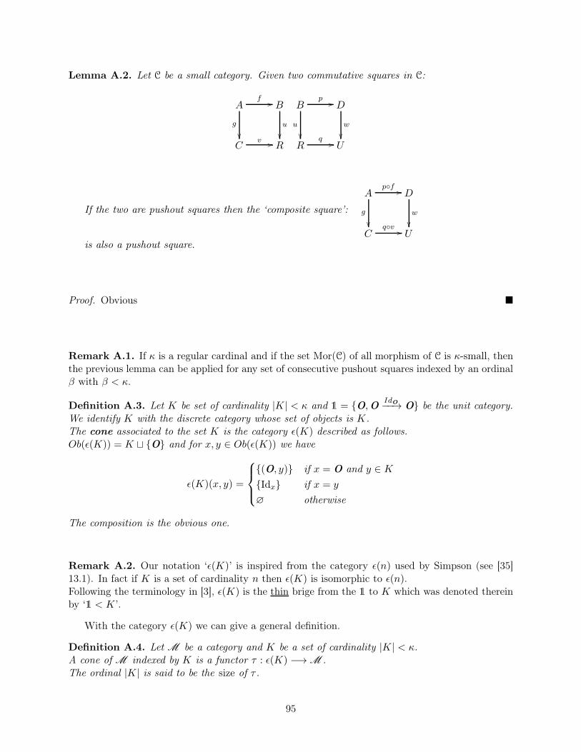
Lemma A.2. Let C be a small category. Given two commutative squares in C:

A B

C R

f //

g

��u

��v //

B D

R U

p //

u

��w

��q //

If the two are pushout squares then the ‘composite square’:

A D

C U

p◦f //

g

��w

��q◦v //

is also a pushout square.

Proof. Obvious �

Remark A.1. If κ is a regular cardinal and if the set Mor(C) of all morphism of C is κ-small, thenthe previous lemma can be applied for any set of consecutive pushout squares indexed by an ordinalβ with β < κ.

Definition A.3. Let K be set of cardinality |K| < κ and 1 = {O,OIdO−−→ O} be the unit category.

We identify K with the discrete category whose set of objects is K.The cone associated to the set K is the category ǫ(K) described as follows.Ob(ǫ(K)) = K ⊔ {O} and for x, y ∈ Ob(ǫ(K)) we have

ǫ(K)(x, y) =

{(O, y)} if x = O and y ∈ K

{Idx} if x = y

∅ otherwise

The composition is the obvious one.

Remark A.2. Our notation ‘ǫ(K)’ is inspired from the category ǫ(n) used by Simpson (see [35]13.1). In fact if K is a set of cardinality n then ǫ(K) is isomorphic to ǫ(n).Following the terminology in [3], ǫ(K) is the thin brige from the 1 to K which was denoted thereinby ‘1 < K’.

With the category ǫ(K) we can give a general definition.

Definition A.4. Let M be a category and K be a set of cardinality |K| < κ.A cone of M indexed by K is a functor τ : ǫ(K) −→M .The ordinal |K| is said to be the size of τ .

95

Concretely a cone of M corresponds to a K-indexed family {A −→ Bk}k∈K of morphisms ofM having the same domain. We can write

τ = {A −→ Bk}k∈K

with A = τ(O), Bk = τ(k) and τ [(O, k)] = A −→ Bk.

Terminology.

• If M is a model category then a cone τ = {A −→ Bk}k∈K is said to be a cone of cofibra-tions if every morphism A −→ Bk is a cofibration.

• More generally given a class of maps I of a category M , a cone τ = {A −→ Bk}k∈K is saidto be a cone of I if every map A −→ Bk is a member of I.

• A cone τ : ǫ(K) −→M is said to be small if the index set K is such that |K| < κ for someregular cardinal κ.

Definition A.5. Let M be a category.A generalized pushout diagram in M is a colimit of a cone τ of M . Here the colimit is thecolimit of the functor τ .

One can check that for a cone τ associated to a set K of cardinality 2, then the colimit of thediagram τ is given by a classical pushout square.

Using the fact that in a model category, the pushout of a cofibration is again a cofibration wehave the following lemma.

Lemma A.6. Let κ be regular cardinal. For any κ-small model category M the following hold.

1. Every small cone τ of M has a colimit.

2. If τ = {A → Bk}k∈K if a cone of (trivial) cofibrations then all the canonical maps:

Bk −→ colim(τ)

A −→ colim(τ)

are also (trivial) cofibrations.

Sketch of proof. The assertion (1) follows from the fact that M has all small colimits by definitionof a model category.

For the assertion (2) it suffices to prove that the canonical map Bk −→ colim(τ) is a (triv-ial) cofibration for every k. The map A −→ colim(τ) which is the composite of A → Bk andBk −→ colim(τ), will be automatically a (trivial) cofibration since (trivial) cofibrations are stableby composition. For the rest of the proof we will simply treat the trivial cofibration case; the othercase is implicitely proved by the same method.

We proceed by induction on the cardinality of K.

96

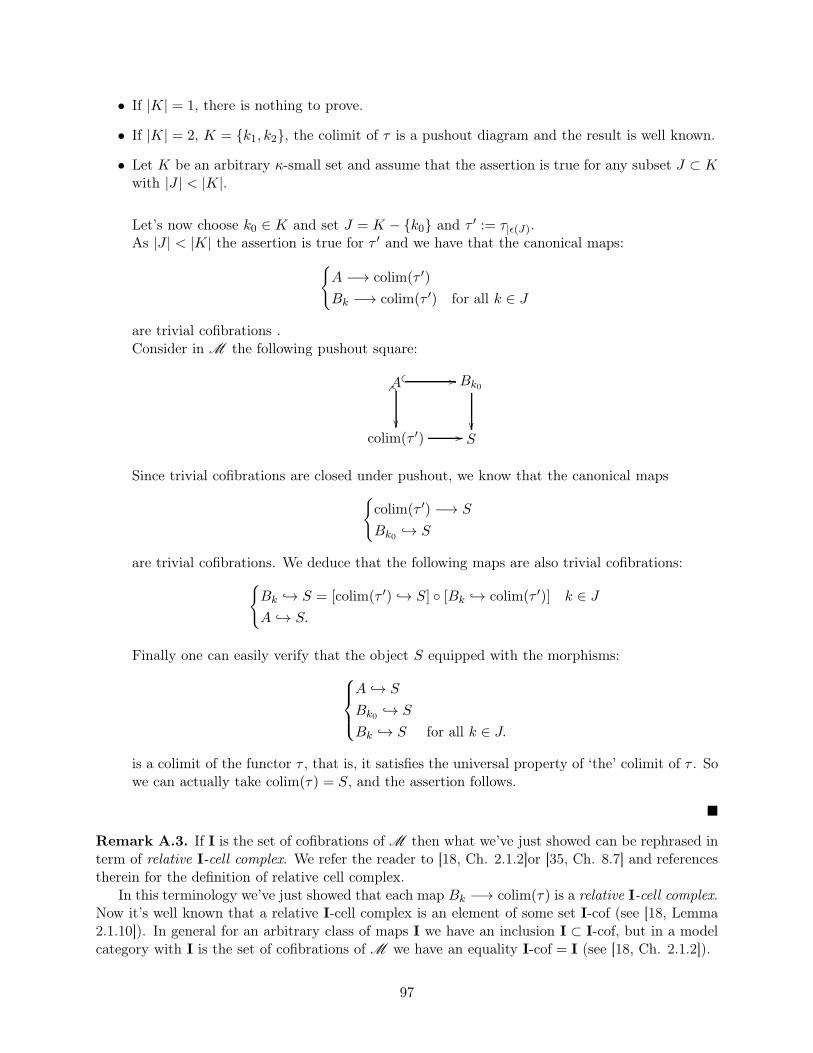
• If |K| = 1, there is nothing to prove.

• If |K| = 2, K = {k1, k2}, the colimit of τ is a pushout diagram and the result is well known.

• Let K be an arbitrary κ-small set and assume that the assertion is true for any subset J ⊂ Kwith |J | < |K|.

Let’s now choose k0 ∈ K and set J = K − {k0} and τ ′ := τ|ǫ(J).As |J | < |K| the assertion is true for τ ′ and we have that the canonical maps:

{A −→ colim(τ ′)

Bk −→ colim(τ ′) for all k ∈ J

are trivial cofibrations .Consider in M the following pushout square:

A Bk0

colim(τ ′) S

� � //_�

�� ��//

Since trivial cofibrations are closed under pushout, we know that the canonical maps

{colim(τ ′) −→ S

Bk0 → S

are trivial cofibrations. We deduce that the following maps are also trivial cofibrations:

{Bk → S = [colim(τ ′) → S] ◦ [Bk → colim(τ ′)] k ∈ J

A → S.

Finally one can easily verify that the object S equipped with the morphisms:

A → S

Bk0 → S

Bk → S for all k ∈ J.

is a colimit of the functor τ , that is, it satisfies the universal property of ‘the’ colimit of τ . Sowe can actually take colim(τ) = S, and the assertion follows.

�

Remark A.3. If I is the set of cofibrations of M then what we’ve just showed can be rephrased interm of relative I-cell complex. We refer the reader to [18, Ch. 2.1.2]or [35, Ch. 8.7] and referencestherein for the definition of relative cell complex.

In this terminology we’ve just showed that each map Bk −→ colim(τ) is a relative I-cell complex.Now it’s well known that a relative I-cell complex is an element of some set I-cof (see [18, Lemma2.1.10]). In general for an arbitrary class of maps I we have an inclusion I ⊂ I-cof, but in a modelcategory with I is the set of cofibrations of M we have an equality I-cof = I (see [18, Ch. 2.1.2]).

97

B Adjunction Lemma

B.1 Lemma 1

In the following we fix M a cocomplete a symmetric closed monoidal category.We remind the reader that being symmetric closed implies that the tensor product commutes withcolimits on both sides. In particular for every (small) diagram D : J −→ M , with J a discretecategory i.e a set, then we have:

[∐

j∈J

D(j)] ⊗ P ∼=∐

j∈J

[D(j) ⊗ P ]

P ⊗ [∐

j∈J

D(j)] ∼=∐

j∈J

[P ⊗D(j)].

Let X nonempty κ-small set and U : MS(X) −→∏

(A,B)∈X2 Hom[SX(A,B)op,M ] be the functordefined as follows.

{U(F ) = {FAB}(A,B)∈X2 for F = {FAB , ϕs,t}(A,B)∈X2 ∈MS(X)

U(σ) = {σAB : FAB −→ GAB}(A,B)∈X2 for Fσ−→ G

So concretely the functor U forgets the laxity maps ‘ϕs,t’.

Our goal is to prove the following lemma.

Lemma B.1. The functor U has a left adjoint, that is there exists a functor

Γ :∏

(A,B)∈X2

Hom[SX(A,B)op,M ] −→MS(X)

such that for all F ∈MS(X) and all X ∈∏

(A,B)∈X2 Hom[SX(A,B)op,M ], we have an isomorphismof set:

Hom[Γ[X ], F ] ∼= Hom[X ,U(F )]

which is natural in F and X .

We will adopt the following conventions.

Conventions.

• If (U1, · · · , Un) is a n-tuple of objects of M we will write U1⊗ · · · ⊗Un for the tensor productof U1, · · · , Un with all pairs of parentheses starting in front.

• For a nonempty set J and J1, J2 two nonempty subsets of J such that J1⊔J2 = J then

for every family (Uj)j∈J of objects of M we will freely identify the two objects∐j∈J Uj and

(∐j∈J1

Uj)∐(∐j∈J2

Uj) and we will call it “the” coproduct of the Uj.

98

In particular for each k ∈ J1, the three canonical maps

ik : Uk −→∐j∈J Uj

iJ1 :∐j∈J1

Uj −→∐j∈J Uj

ik,J1 : Uk −→∐j∈J1

Uj

are linked by the equality: ik = iJ1 ◦ ik,J1 .

Before giving the proof we make some few observations.

Observations 5. Let (A,B) be a pair of elements of X and t ∈ SX(A,B). Denote by d the degree(or length) of t.

Consider the set Dec(t) of all decompositions or ‘presentations’ of t given by:

Dec(t) =∐

0≤l≤d−1

{(t0, · · · , tl),with t0 ⊗ · · · ⊗ tl = t}

where for l = 0 we have t0 = tl = t.

Given t′ ∈ SX(A,B) of length d′ and a morphism u : t −→ t′ (hence d′ ≤ d) then for any(t′0, · · · , t

′l) ∈ Dec(t′), there exists a unique (t0, · · · , tl) ∈ Dec(t) together with a unique (l+1)-tuple

of morphisms (u0, · · · , ul) with ui : ti −→ t′i such that:

u = u0 ⊗ · · · ⊗ ul.

This follows from the fact in SX the composition is a concatenation of chains ‘side by side’ whichis a generalization of the ordinal addition in (∆epi,+, 0). In fact by construction each SX(A,B) isa category of elements of a functor from ∆epi to the category of sets. In particular the morphismsin SX(A,B) are parametrized by the morphism of ∆epi and we clearly have this property of decom-position of morphisms in (∆epi,+).

It follows that any map u : t −→ t′ of SX(A,B) determines a unique function Dec(u) :Dec(t′) −→ Dec(t). Moreover it’s not hard to see that if we have two composable maps u : t −→ t′,u′ : t′ −→ t′′ then Dec(u′ ◦ u) = Dec(u′) ◦Dec(u).

Remark B.1. One can observe that for t ∈ SX(A,B) and s ∈ SX(B,C) we have a canonical mapof sets

Dec(s)×Dec(t) −→ Dec(s⊗ t)

which is injective, so that we can view Dec(s)×Dec(t) as a subset of Dec(s⊗ t).And more generally for each (t0, · · · , tl) ∈ Dec(t) with l > 0 we can identify Dec(t0)× · · · ×Dec(tl)with a subset of Dec(t).

99

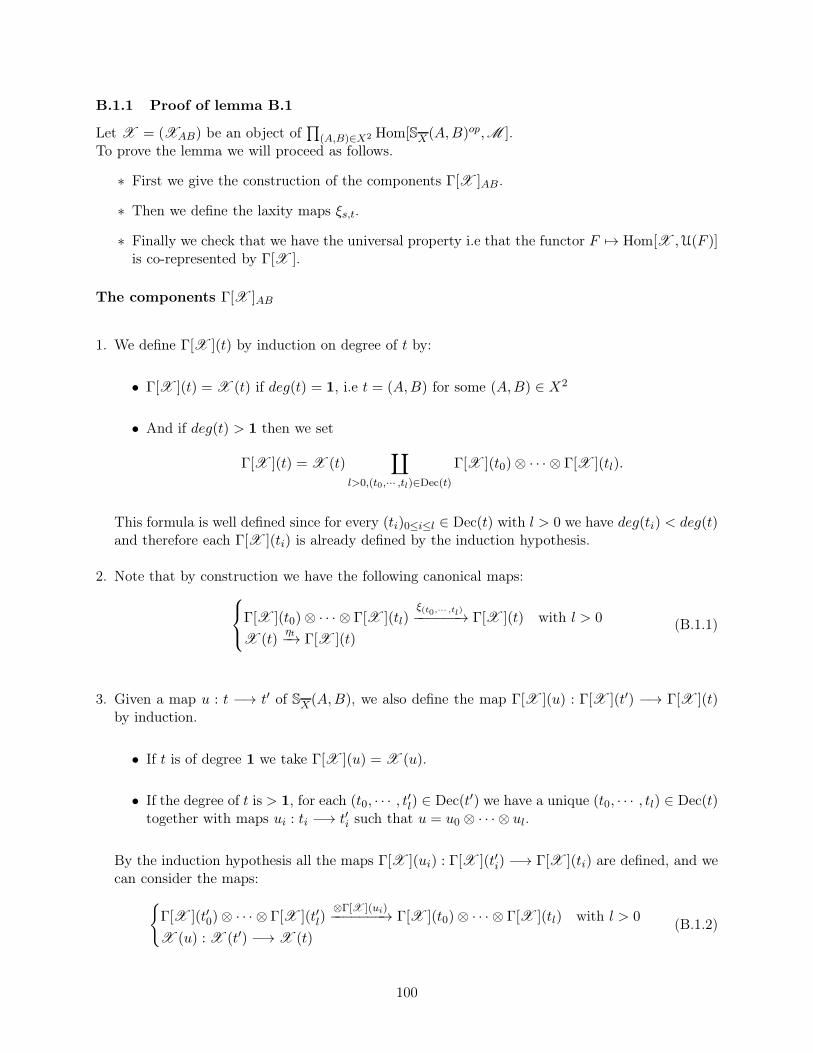
B.1.1 Proof of lemma B.1

Let X = (XAB) be an object of∏

(A,B)∈X2 Hom[SX(A,B)op,M ].To prove the lemma we will proceed as follows.

∗ First we give the construction of the components Γ[X ]AB .

∗ Then we define the laxity maps ξs,t.

∗ Finally we check that we have the universal property i.e that the functor F 7→ Hom[X ,U(F )]is co-represented by Γ[X ].

The components Γ[X ]AB

1. We define Γ[X ](t) by induction on degree of t by:

• Γ[X ](t) = X (t) if deg(t) = 1, i.e t = (A,B) for some (A,B) ∈ X2

• And if deg(t) > 1 then we set

Γ[X ](t) = X (t)∐

l>0,(t0,··· ,tl)∈Dec(t)

Γ[X ](t0)⊗ · · · ⊗ Γ[X ](tl).

This formula is well defined since for every (ti)0≤i≤l ∈ Dec(t) with l > 0 we have deg(ti) < deg(t)and therefore each Γ[X ](ti) is already defined by the induction hypothesis.

2. Note that by construction we have the following canonical maps:

Γ[X ](t0)⊗ · · · ⊗ Γ[X ](tl)

ξ(t0,··· ,tl)−−−−−−→ Γ[X ](t) with l > 0

X (t)ηt−→ Γ[X ](t)

(B.1.1)

3. Given a map u : t −→ t′ of SX(A,B), we also define the map Γ[X ](u) : Γ[X ](t′) −→ Γ[X ](t)by induction.

• If t is of degree 1 we take Γ[X ](u) = X (u).

• If the degree of t is > 1, for each (t0, · · · , t′l) ∈ Dec(t′) we have a unique (t0, · · · , tl) ∈ Dec(t)

together with maps ui : ti −→ t′i such that u = u0 ⊗ · · · ⊗ ul.

By the induction hypothesis all the maps Γ[X ](ui) : Γ[X ](t′i) −→ Γ[X ](ti) are defined, and wecan consider the maps:

{Γ[X ](t′0)⊗ · · · ⊗ Γ[X ](t′l)

⊗Γ[X ](ui)−−−−−−−→ Γ[X ](t0)⊗ · · · ⊗ Γ[X ](tl) with l > 0

X (u) : X (t′) −→X (t)(B.1.2)

100

The composite of the maps in (B.1.2) followed by the maps in (B.1.1) gives the following

Γ[X ](t′0)⊗ · · · ⊗ Γ[X ](t′l)

ξ(t0,··· ,tl)◦(⊗Γ[X ](ui))−−−−−−−−−−−−−−→ Γ[X ](t) with l > 0

X (t′)ηt◦X (u)−−−−−→ Γ[X ](t)

(B.1.3)

Finally using the universal property of the coproduct, we know that the maps in (B.1.3) deter-mines a unique map:

Γ[X ]AB(u) : Γ[X ]AB(t′) −→ Γ[X ]AB(t).

4. It’s not hard to check that these data determine a functor Γ[X ]AB : SX(A,B)op −→M .

5. We leave the reader to check that all the maps in (B.1.1) are natural in all variable ti includingt. In particular the maps ηt determine a natural transformation

ηAB : XAB −→ Γ[X ]AB

These natural transformations {ηAB}(A,B)∈X2 will constitute the unity of the adjunction.

Remark B.2. We can define alternatively Γ[X ] without using induction by the formula:

Γ[X ](t) =∐

(t0,··· ,tl)∈Dec(t)

X (t0)⊗ · · · ⊗X (tl).

where we include also the case l = 0 to have X (t) in the coproduct.

It’s not hard to check that the Γ[X ] we get by this formula and the previous one are naturallyisomorphic. But for simplicity we will work with the definition by induction.

The laxity maps The advantage of the definition by induction is that we have ‘on the nose’ thelaxity maps which correspond to the canonical maps :

Γ[X ](s)⊗ Γ[X ](t)ξs,t

−−−−−−−−−→(s,t)∈Dec(s⊗t)

Γ[X ](s ⊗ t)

for all pair of composable morphisms (s, t). And one can check that these laxity maps satisfy thecoherence axioms of a lax morphism, so that Γ[X ] is indeed an SX-diagram.

Given two objects X , X ′ with a morphism δ : X −→X ′, one defines Γ(δ) = {Γ(δ)t} with:

Γ(δ)t = δt∐

(t0,··· ,tl)∈Dec(t),l>0

Γ(δ)t0 ⊗ · · · ⊗ Γ(δ)tl .

We leave the reader check that Γ is a functor.

101

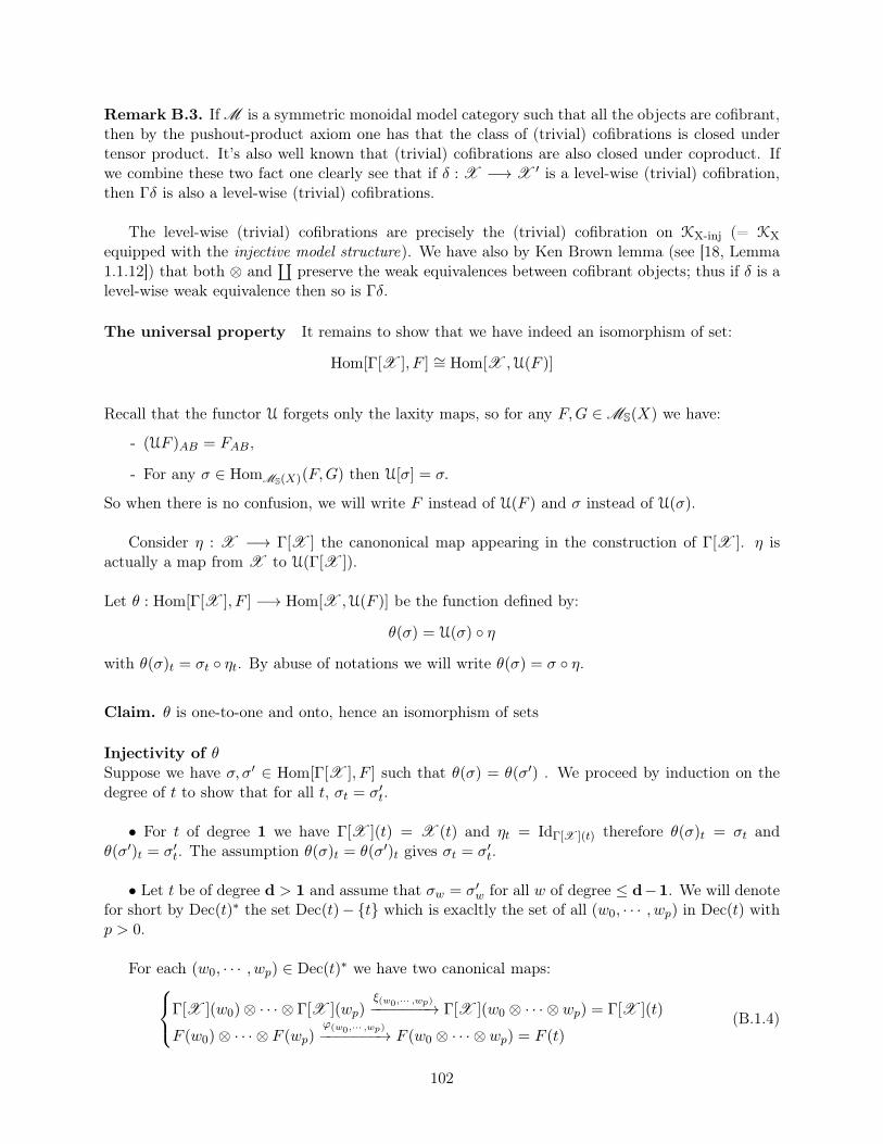
Remark B.3. If M is a symmetric monoidal model category such that all the objects are cofibrant,then by the pushout-product axiom one has that the class of (trivial) cofibrations is closed undertensor product. It’s also well known that (trivial) cofibrations are also closed under coproduct. Ifwe combine these two fact one clearly see that if δ : X −→ X ′ is a level-wise (trivial) cofibration,then Γδ is also a level-wise (trivial) cofibrations.

The level-wise (trivial) cofibrations are precisely the (trivial) cofibration on KX-inj (= KX

equipped with the injective model structure). We have also by Ken Brown lemma (see [18, Lemma1.1.12]) that both ⊗ and

∐preserve the weak equivalences between cofibrant objects; thus if δ is a

level-wise weak equivalence then so is Γδ.

The universal property It remains to show that we have indeed an isomorphism of set:

Hom[Γ[X ], F ] ∼= Hom[X ,U(F )]

Recall that the functor U forgets only the laxity maps, so for any F,G ∈MS(X) we have:

- (UF )AB = FAB ,

- For any σ ∈ HomMS(X)(F,G) then U[σ] = σ.

So when there is no confusion, we will write F instead of U(F ) and σ instead of U(σ).

Consider η : X −→ Γ[X ] the canononical map appearing in the construction of Γ[X ]. η isactually a map from X to U(Γ[X ]).

Let θ : Hom[Γ[X ], F ] −→ Hom[X ,U(F )] be the function defined by:

θ(σ) = U(σ) ◦ η

with θ(σ)t = σt ◦ ηt. By abuse of notations we will write θ(σ) = σ ◦ η.

Claim. θ is one-to-one and onto, hence an isomorphism of sets

Injectivity of θSuppose we have σ, σ′ ∈ Hom[Γ[X ], F ] such that θ(σ) = θ(σ′) . We proceed by induction on thedegree of t to show that for all t, σt = σ′t.

• For t of degree 1 we have Γ[X ](t) = X (t) and ηt = IdΓ[X ](t) therefore θ(σ)t = σt andθ(σ′)t = σ′t. The assumption θ(σ)t = θ(σ′)t gives σt = σ′t.

• Let t be of degree d > 1 and assume that σw = σ′w for all w of degree ≤ d−1. We will denotefor short by Dec(t)∗ the set Dec(t)−{t} which is exacltly the set of all (w0, · · · , wp) in Dec(t) withp > 0.

For each (w0, · · · , wp) ∈ Dec(t)∗ we have two canonical maps:Γ[X ](w0)⊗ · · · ⊗ Γ[X ](wp)

ξ(w0,··· ,wp)−−−−−−−→ Γ[X ](w0 ⊗ · · · ⊗ wp) = Γ[X ](t)

F (w0)⊗ · · · ⊗ F (wp)ϕ(w0,··· ,wp)−−−−−−−→ F (w0 ⊗ · · · ⊗ wp) = F (t)

(B.1.4)

102

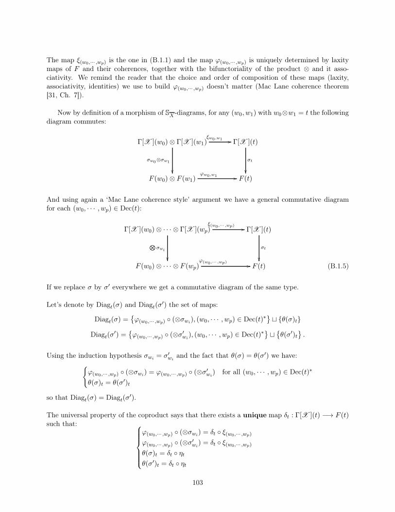
The map ξ(w0,··· ,wp) is the one in (B.1.1) and the map ϕ(w0,··· ,wp) is uniquely determined by laxitymaps of F and their coherences, together with the bifunctoriality of the product ⊗ and it asso-ciativity. We remind the reader that the choice and order of composition of these maps (laxity,associativity, identities) we use to build ϕ(w0,··· ,wp) doesn’t matter (Mac Lane coherence theorem[31, Ch. 7]).

Now by definition of a morphism of SX-diagrams, for any (w0, w1) with w0⊗w1 = t the followingdiagram commutes:

Γ[X ](w0)⊗ Γ[X ](w1) Γ[X ](t)

F (w0)⊗ F (w1) F (t)

ξw0,w1 //

σw0⊗σw1

��

σt

��ϕw0,w1 //

And using again a ‘Mac Lane coherence style’ argument we have a general commutative diagramfor each (w0, · · · , wp) ∈ Dec(t):

Γ[X ](w0)⊗ · · · ⊗ Γ[X ](wp) Γ[X ](t)

F (w0)⊗ · · · ⊗ F (wp) F (t)

ξ(w0,··· ,wp) //

⊗σwi

��

σt

��ϕ(w0,··· ,wp) // (B.1.5)

If we replace σ by σ′ everywhere we get a commutative diagram of the same type.

Let’s denote by Diagt(σ) and Diagt(σ′) the set of maps:

Diagt(σ) ={ϕ(w0,··· ,wp) ◦ (⊗σwi), (w0, · · · , wp) ∈ Dec(t)∗

}⊔ {θ(σ)t}

Diagt(σ′) =

{ϕ(w0,··· ,wp) ◦ (⊗σ

′wi), (w0, · · · , wp) ∈ Dec(t)∗

}⊔{θ(σ′)t

}.

Using the induction hypothesis σwi = σ′wiand the fact that θ(σ) = θ(σ′) we have:

{ϕ(w0,··· ,wp) ◦ (⊗σwi) = ϕ(w0,··· ,wp) ◦ (⊗σ

′wi) for all (w0, · · · , wp) ∈ Dec(t)∗

θ(σ)t = θ(σ′)t

so that Diagt(σ) = Diagt(σ′).

The universal property of the coproduct says that there exists a unique map δt : Γ[X ](t) −→ F (t)such that:

ϕ(w0,··· ,wp) ◦ (⊗σwi) = δt ◦ ξ(w0,··· ,wp)

ϕ(w0,··· ,wp) ◦ (⊗σ′wi) = δt ◦ ξ(w0,··· ,wp)

θ(σ)t = δt ◦ ηt

θ(σ′)t = δt ◦ ηt

103

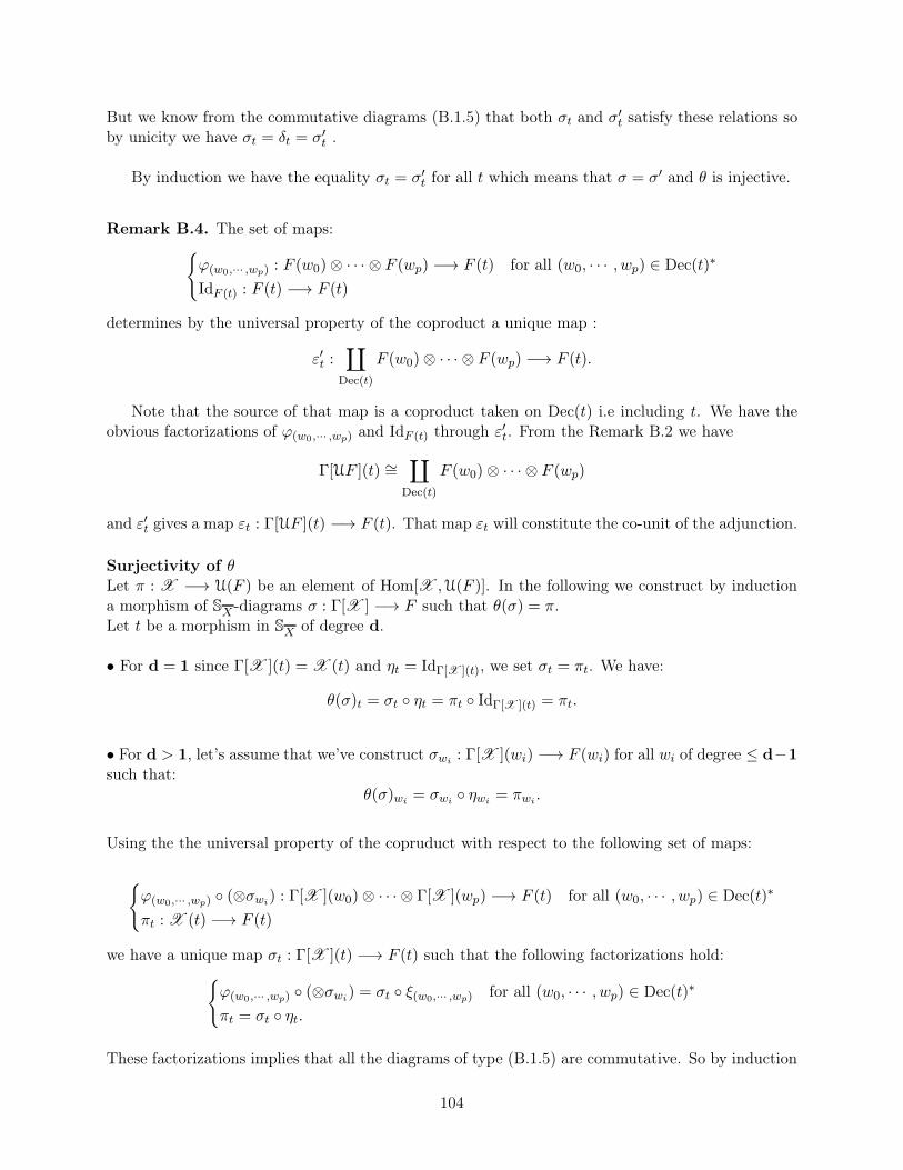
But we know from the commutative diagrams (B.1.5) that both σt and σ′t satisfy these relations soby unicity we have σt = δt = σ′t .

By induction we have the equality σt = σ′t for all t which means that σ = σ′ and θ is injective.

Remark B.4. The set of maps:{ϕ(w0,··· ,wp) : F (w0)⊗ · · · ⊗ F (wp) −→ F (t) for all (w0, · · · , wp) ∈ Dec(t)∗

IdF (t) : F (t) −→ F (t)

determines by the universal property of the coproduct a unique map :

ε′t :∐

Dec(t)

F (w0)⊗ · · · ⊗ F (wp) −→ F (t).

Note that the source of that map is a coproduct taken on Dec(t) i.e including t. We have theobvious factorizations of ϕ(w0,··· ,wp) and IdF (t) through ε′t. From the Remark B.2 we have

Γ[UF ](t) ∼=∐

Dec(t)

F (w0)⊗ · · · ⊗ F (wp)

and ε′t gives a map εt : Γ[UF ](t) −→ F (t). That map εt will constitute the co-unit of the adjunction.

Surjectivity of θLet π : X −→ U(F ) be an element of Hom[X ,U(F )]. In the following we construct by inductiona morphism of SX-diagrams σ : Γ[X ] −→ F such that θ(σ) = π.Let t be a morphism in SX of degree d.

• For d = 1 since Γ[X ](t) = X (t) and ηt = IdΓ[X ](t), we set σt = πt. We have:

θ(σ)t = σt ◦ ηt = πt ◦ IdΓ[X ](t) = πt.

• For d > 1, let’s assume that we’ve construct σwi : Γ[X ](wi) −→ F (wi) for all wi of degree ≤ d−1such that:

θ(σ)wi = σwi ◦ ηwi = πwi .

Using the the universal property of the copruduct with respect to the following set of maps:

{ϕ(w0,··· ,wp) ◦ (⊗σwi) : Γ[X ](w0)⊗ · · · ⊗ Γ[X ](wp) −→ F (t) for all (w0, · · · , wp) ∈ Dec(t)∗

πt : X (t) −→ F (t)

we have a unique map σt : Γ[X ](t) −→ F (t) such that the following factorizations hold:

{ϕ(w0,··· ,wp) ◦ (⊗σwi) = σt ◦ ξ(w0,··· ,wp) for all (w0, · · · , wp) ∈ Dec(t)∗

πt = σt ◦ ηt.

These factorizations implies that all the diagrams of type (B.1.5) are commutative. So by induction

104

for all t we have these commutative diagrams which gives the required axioms for transformationsof lax-morphisms (see Definition 4.13).

Moreover we clear have by construction that θ(σ)t = σt ◦ ηt = πt for all t, that is θ(σ) = π andθ is surjective.

We leave the reader to check that all the constructions considered in the previous paragraphsare natural in both X and F . �

B.2 Evaluations on morphism have left adjoint

In the following M represents a cocomplete category. Given a small category C and a morphismα of C we will denote by Evα : Hom(C,M ) −→M [1] the functor that takes F ∈ Hom(C,M ) to F(α).

Let [1] = (0 −→ 1) be the interval category. A morphism α of C can be identified with a functordenoted again α : [1] −→ C, that takes 0 to the source of α and 1 to the target.

Then we can identify Evα with the pullback functor α⋆ : Hom(C,M)α◦−→ Hom([1],M ) = M 2. With

this identification one easily establish that

Lemma B.2. For a small category C and any morphism α ∈ C the functor Evα has a left adjointFα : M [1] −→ Hom(C,M ).

Proof. This is a special case of a more general situation where we have a functor α : B −→ C; theleft adjoint of α⋆ is α! which corresponds to the left Kan extension functor along α. The reader canfind a detailed proof for example in [29, A.2.8.7], [35, Ch. 7.6.1], [17, Ch. 11.6]. �

Corollary B.3. Fα is a left Quillen functor between the corresponding projective model structures.

Proof. A left adjoint is a left Quillen functor if and only if its right adjoint is a right Quillen functor(see lemma [18, 1.3.4]); consequently Fα is a left Quillen functor if and only if Evα is a right Quillenfunctor.

But in the respective projective model structure on Hom(C,M ) and M [1] = Hom([1],M ), the(trivial) fibrations are the level-wise ones, so Evα clearly preserves them. Thus Evα is a right Quillenfunctor and the result follows. �

Remark B.5. From Ken Brown lemma ([18, Lemma 1.1.12]), Fα preserves weak equivalencesbetween cofibrant objects. Recall that a cofibrant object in M 2

proj is a cofibration in M with acofibrant domain. In particular if all the objects of M are cofibrant, then the cofibrant objects inM 2

proj are simply all the cofibrations of M . Therefore if all the objects of M are cofibrant then Fα

preserves weak equivalence between any two cofibrations.

Our main interest in the above lemma is when C = SX(A,B)op and α = ut, the unique morphismin SX(A,B)op from (A,B) to t (see Observation 2).

Each category SX(A,B)op is an example of direct category, that is a a category C equiped witha linear extension functor deg : C −→ λ, where λ is an ordinal. One requires furthermore that degtakes nonidentiy maps to nonidentiy maps; this way any nonidentity map raises the degree. Notethat SX(A,B)op has an initial object e which corresponds to (A,B).

For such categories C one has the following

105

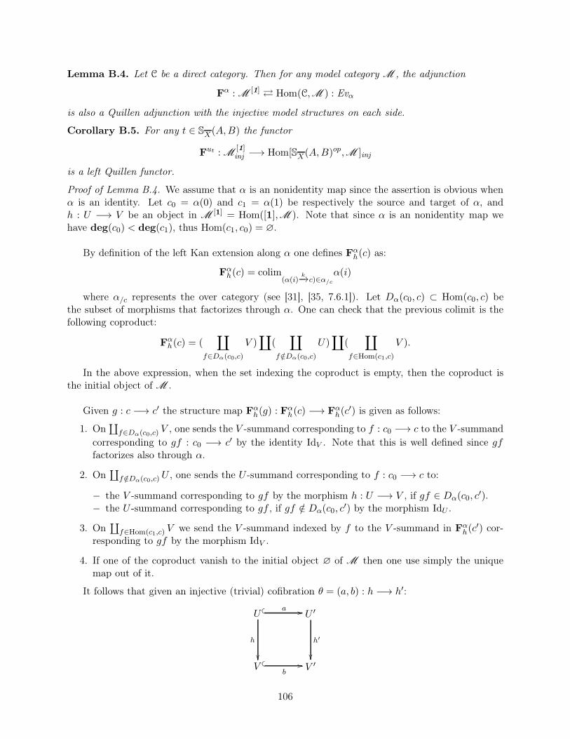
Lemma B.4. Let C be a direct category. Then for any model category M , the adjunction

Fα : M[1]⇄ Hom(C,M ) : Evα

is also a Quillen adjunction with the injective model structures on each side.

Corollary B.5. For any t ∈ SX(A,B) the functor

Fut : M[1]inj −→ Hom[SX(A,B)op,M ]inj

is a left Quillen functor.

Proof of Lemma B.4. We assume that α is an nonidentity map since the assertion is obvious whenα is an identity. Let c0 = α(0) and c1 = α(1) be respectively the source and target of α, andh : U −→ V be an object in M [1] = Hom([1],M ). Note that since α is an nonidentity map wehave deg(c0) < deg(c1), thus Hom(c1, c0) = ∅.

By definition of the left Kan extension along α one defines Fαh(c) as:

Fαh(c) = colim(α(i)

k−→c)∈α/c

α(i)

where α/c represents the over category (see [31], [35, 7.6.1]). Let Dα(c0, c) ⊂ Hom(c0, c) bethe subset of morphisms that factorizes through α. One can check that the previous colimit is thefollowing coproduct:

Fαh(c) = (∐

f∈Dα(c0,c)

V )∐

(∐

f /∈Dα(c0,c)

U)∐

(∐

f∈Hom(c1,c)

V ).

In the above expression, when the set indexing the coproduct is empty, then the coproduct isthe initial object of M .

Given g : c −→ c′ the structure map Fαh(g) : Fαh(c) −→ Fαh(c

′) is given as follows:

1. On∐f∈Dα(c0,c)

V , one sends the V -summand corresponding to f : c0 −→ c to the V -summand

corresponding to gf : c0 −→ c′ by the identity IdV . Note that this is well defined since gffactorizes also through α.

2. On∐f /∈Dα(c0,c)

U , one sends the U -summand corresponding to f : c0 −→ c to:

− the V -summand corresponding to gf by the morphism h : U −→ V , if gf ∈ Dα(c0, c′).

− the U -summand corresponding to gf , if gf /∈ Dα(c0, c′) by the morphism IdU .

3. On∐f∈Hom(c1,c)

V we send the V -summand indexed by f to the V -summand in Fαh(c′) cor-

responding to gf by the morphism IdV .

4. If one of the coproduct vanish to the initial object ∅ of M then one use simply the uniquemap out of it.

It follows that given an injective (trivial) cofibration θ = (a, b) : h −→ h′:

U U ′

V V ′

� � a //

h

��� �

b//

h′

��

106

the c-component of Fαθ is the coproduct

Fαθ,c = (∐

f∈Dα(c0,c)

b)∐

(∐

f /∈Dα(c0,c)

a)∐

(∐

f∈Hom(c1,c)

b).

Since (trivial) cofibrations are closed under coproduct we deduce that Fαθ,c is a (trivial) cofibrationif θ is so, thus Fα is a left Quillen functor as desired. �

C MS(X) is cocomplete if M is so

In this section we want to prove the following

Theorem C.1. Given a co-complete symmetric monoidal category M , for any nonempty set X thecategory MS(X) is co-complete.

The proof of this theorem follows exactly the same ideas as the proof of the co-completeness ofM -Cat given by Wolff [39].

We will proceed as follows.

• We will show first that MS(X) is monadic over KX =∏

(A,B)∈X2 Hom[SX(A,B)op,M ] usingthe Beck monadicity theorem [?].

• As the adjunction is monadic we know that MS(X) has a coequalizers of U-split pair ofmorphisms and preserve them.

• Since KX is cocomplete by a result of Linton [28, Corollary 2] the cateogry of algebra of themonad, which is equivalent to MS(X), is cocomplete.

C.1 MS(X) has coequalizers of reflexive pairs

The question of existence of coequalizers in MS(X) is similar to that of coequalizers in M -Cat

which was treated by Wolff [39]. For our needs we only treat the question of coequalizer of reflexivepairs.Given a parallel pair of morphisms in MS(X) (σ1, σ2) : D ⇒ F one can view it as defining a‘relation’ ‘R = Im(σ1 × σ2) ⊂ F × F ’ on F . We will call such relation ‘precongruence’. In thissituation the question is to find out when a quotient object ‘E = F/R’ (‘the coequalizer’) exists inMS(X). We will proceed in the same maner as Wolff; below we outline the different steps beforegoing to details.

1. We will start by giving a criterion which says under which conditions the coequalizer computedin KX lifts to a coequalizer in MS(X).

2. When a parallel pair of morphisms is a reflexive pair (=the analogue of the relation R tobe reflexive) we will show that the conditions of the criterion are fullfiled and the result willfollow.

107

C.1.1 Lifting of coequalizer

Definition C.2. Let F be an object of MS(X).

1. A precongruence in F is a pair of parallel morphisms in KX

A UFσ1

//σ2 //

for some object A ∈ KX .

2. Let E be a coequalizer in KX of (σ1, σ2), with L : UF −→ E the canonical map. We say thatthe precongruence is a congruence if:

• E = U(E) for some E ∈MS(X) and

• L = U(L) for a (unique) morphism L : F −→ E in MS(X).

When there is no confusion we simply write E for E and L for L.

Lemma C.3. Let F be an object of MS(X) and consider a precongruence:

A UF Eσ1

//σ2 // L //

Denote by ϕs,t : F (s)⊗ F (t) −→ F (s⊗ t) be the laxity maps of F .

Then the precongruence is a congruence if and only if for any pair (s, t) of composable 1-morphismsin SX the following equalities hold:

Ls⊗t ◦ [ϕs,t ◦ (IdF (s)⊗σ1(t))] = Ls⊗t ◦ [ϕs,t ◦ (IdF (s)⊗σ2(t))]

Ls⊗t ◦ [ϕs,t ◦ (σ1(s)⊗ IdF (t))] = Ls⊗t ◦ [ϕs,t ◦ (σ2(s)⊗ IdF (t))].

In this case the structure of SX-diagram on E is unique.

Remark C.1. If F was (the nerve of) an M -category, taking s = (A,B), and t = (B,C), we haves ⊗ t = (B,C) and the laxity maps correpond to the composition: cABC : F (A,B) ⊗ F (B,C) −→F (A,C). One can check that the previous conditions are the same as in [39, Lemma 2.7].

Sketch of proof. The fact that having a congruence implies the equalities is easy and follows fromthe fact that L is a morphism in MS(X) and that L is a coequalizer of σ1 and σ2. We will thenonly prove that the equalities force a congruence.

To prove the statement we need to provide the laxity maps for E: φs,t : E(s)⊗E(t) −→ E(s⊗t).By definition of E, for any 1-morphism s ∈ SX , E(s) is a coequalizer of (σ1(s), σ2(s)), which is aparticular case of colimit in M . Since M is a symmetric monoidal closed, colimits commute on eachfactor with the tensor product ⊗ of M . It follows that given a pair (s, t) of composable morphismsthen E(s)⊗ E(t) is the colimit of the ‘diagram’:

ǫ(s, t) = {A(s)⊗A(t)σi(s)⊗σj (t)−−−−−−−→ F (s)⊗ F (t)}i,j∈{1,2}.

108

Now we claim that all the composite Ls⊗t ◦ϕs,t ◦ [σi(s)⊗σj(t)] : A(s)⊗A(t) −→ E(s⊗ t) are equal.This equivalent to say that the diagram

ǫ′(s, t) = Ls⊗t ◦ ϕs,t ◦ ǫ(s, t) := {Ls⊗t ◦ ϕs,t ◦ [σi(s)⊗ σj(t)]}i,j∈{1,2}

is a compatible cocone. Before telling why this is true let’s see how we get the laxity maps for E.For that it suffices to observe that since ǫ′(s, t) := Ls⊗t ◦ϕs,t ◦ ǫ(s, t) is a compatible cocone, by theuniversal property of the colimit of ǫ(s, t) there exists a unique map ψs,t : E(s)⊗E(t) −→ E(s⊗ t)making the obvious diagrams commutative. In particular for any s, t the following is commutative:

F (s)⊗ F (t) F (s⊗ t)

E(s)⊗ E(t) E(s ⊗ t)

ϕs,t //

Ls⊗Lt

��

Ls⊗t

��ψs,t //❴❴❴❴

The fact that the morphism ψs,t fit coherently is left to the reader as it’s straightforward: itsuffices to introduce a cocone ǫ(s, t, u) whose colimit ‘is’ E(s)⊗ E(t)⊗ E(u) and use the universalproperty of the colimit. This shows that (E,ψs,t) is an object of MS(X) and that L extends to amorphism in MS(X).

Now with some easy but tedious computations one gets successively the desired equalities:

Ls⊗t ◦ ϕs,t ◦ [σ1(s)⊗ σ2(t)] = Ls⊗t ◦ ϕs,t ◦ [(IdF (s)⊗σ2(t)) ◦ (σ1(s)⊗ IdA(t))]

= Ls⊗t ◦ [ϕs,t ◦ (IdF (s)⊗σ2(t))]︸ ︷︷ ︸=Ls⊗t◦[ϕs,t◦(IdF (s) ⊗σ1(t))]

◦(σ1(s)⊗ IdA(t))

(1) = Ls⊗t ◦ [ϕs,t ◦ (IdF (s)⊗σ1(t))] ◦ (σ1(s)⊗ IdA(t))

= Ls⊗t ◦ ϕs,t ◦ [σ1(s)⊗ σ1(t)]

From (1) = Ls⊗t ◦ ϕs,t ◦ [(IdF (s)⊗σ1(t)) ◦ (σ1(s)⊗ IdA(t))]

= Ls⊗t ◦ ϕs,t ◦ [(σ1(s)⊗ IdF (t)) ◦ (IdA(s)⊗σ1(t))]

= Ls⊗t ◦ [ϕs,t ◦ (σ1(s)⊗ IdF (t))]︸ ︷︷ ︸=Ls⊗t◦[ϕs,t◦(σ2(s)⊗IdF (t))]

◦(IdA(s)⊗σ1(t))

(2) = Ls⊗t ◦ [ϕs,t ◦ (σ2(s)⊗ IdF (t))] ◦ (IdA(s)⊗σ1(t))

= Ls⊗t ◦ ϕs,t ◦ [σ2(s)⊗ σ1(t)]

From (2) = Ls⊗t ◦ [ϕs,t ◦ (σ2(s)⊗ IdF (t))] ◦ (IdA(s)⊗σ1(t))

= Ls⊗t ◦ ϕs,t ◦ [(IdF (s)⊗σ1(t)) ◦ (σ2(s)⊗ IdA(t))]

= Ls⊗t ◦ [ϕs,t ◦ (IdF (s)⊗σ1(t))︸ ︷︷ ︸=Ls⊗t◦[ϕs,t◦(IdF (s) ⊗σ2(t))

◦(σ2(s)⊗ IdA(t))

= Ls⊗t ◦ [ϕs,t ◦ (IdF (s)⊗σ2(t)) ◦ (σ2(s)⊗ IdA(t))

= Ls⊗t ◦ ϕs,t ◦ [σ2(s)⊗ σ2(t)]

�

109

Following Linton [28] we introduce the

Definition C.4. Let σ1, σ2 : A ⇒ UF be a parallel pair of morphisms in KX i.e a precongruencein F . We will say that a morphism L : F −→ E in MS(X) is a coequalizer relative to U if:

1. If UL ◦ σ1 = UL ◦ σ2 and

2. if for any morphism L′ : F −→ Z in MS(X) which satisfies UL′ ◦ σ1 = UL′ ◦ σ2 then thereexists a unique morphism H : E −→ Z in MS(X) such that L′ = H ◦ L.

Lemma C.5. If a precongruence

A UF Eσ1

//σ2 // L //

is a congruence then the morphism L : F −→ E is a coequalizer rel. to U.

Proof. Obvious: follows from the construction of (E,ψs,t).�

Lemma C.6 (Linton). Let U : D −→ C be a faithful functor and f , g : A −→ B be a pair of parallel

of morphisms in D. Denote by f = Uf and g = Ug. Then for p : A −→ E in D, the following areequivalent:

• p is a coequalizer of (f , g),

• p is a coequalizer rel. to U of (f, g).

Proof. See [28, Lemma 1]. �

For a given F ∈MS(X), among the precongruences defined in F we have the ones coming fromparallel pair of morphisms in MS(X) namely:

UD UFUσ1

//Uσ2 //

for some D ∈MS(X).

The following lemma tells about these congruences.

Lemma C.7. Let F be an object of MS(X). Consider a precongruence in F

UD UF EUσ1

//Uσ2 // L // .

If there exists a split i.e a morphism p : UF −→ UD in KX such that Uσ1 ◦ p = Uσ2 ◦ p = IdUFthen:

• the precongruence is a congruence and hence

• L : F −→ E is a coequalizer in MS(X) of the pair (σ1, σ2) : D ⇒ F (and is obviously preservedby U).

110

Proof. We will simply need to show that the equalities of Lemma C.3 holds. We will reduce theproof to the first equalities since the second ones are treated in the same manner by simply per-muting IdF ⊗σi to σi ⊗ IdF .

Setting σ1 = Uσ1 and σ2 = Uσ2, these equalities become:

Ls⊗t ◦ [ϕs,t ◦ (IdF (s)⊗σ1(t))] = Ls⊗t ◦ [ϕs,t ◦ (IdF (s)⊗σ2(t))]

And to simplify the notations we will remove the letters ‘s⊗ t, s, t’ but will mention ‘ϕF’ or ‘ϕ

D’

for the laxity maps of F and D repsectively. The previous equality will be then written, when thereis no confusion, as follows:

L ◦ [ϕF◦ (IdF ⊗σ1)] = L ◦ [ϕ

F◦ (IdF ⊗σ2)].

Since σ1 ◦ p = IdF = σ2 ◦ p, we have that

IdF ⊗σ1 = (σ1 ◦ p)⊗ (σ1 ◦ IdD)

= (σ1 ⊗ σ1) ◦ (p ⊗ IdD).

Similarly for σ2: IdF ⊗σ2 = (σ2 ⊗ σ2) ◦ (p⊗ IdD).

With these observations we can compute

L ◦ [ϕF◦ (IdF ⊗σ1)] = L ◦ ϕ

F◦ (σ1 ⊗ σ1) ◦ (p⊗ IdD)

= L ◦ σ1 ◦ ϕD◦ (p⊗ IdD) (a)

= L ◦ σ2 ◦ ϕD◦ (p⊗ IdD) (∗)

= L ◦ ϕF ◦ (σ2 ⊗ σ2) ◦ (p⊗ IdD) (b)

= L ◦ [ϕF◦ (IdF ⊗σ2)]

This gives the desired equalities. We justify the different steps below.

• In (a) and (b) we’ve used the fact that σ1 and σ2 are morphisms in MS(X), which impliesin particluar that

ϕF ◦ (σi ⊗ σi) = σi ◦ ϕD .

This last equality is equivalent to say that the following diagram commutes:

D(s)⊗D(t) D(s⊗ t)

F (s)⊗ F (t) F (s⊗ t)

ϕD //

σi⊗σi

��

σi

��ϕF //❴❴❴❴

• In (∗) we’ve used the fact that L is a coequalizer of σ1 and σ2 therefore: L ◦ σ1 = L ◦ σ2.

Now from the lemma C.5, we know that L is a coequalizer of (Uσ1,Uσ2) rel. to U, since U isclearly faithful Lemma C.6 applies, hence L is a coequalizer in MS(X) of (σ1, σ2) (and is obviouslypreserved by U). �

111

Corollary C.8. MS(X) has coequalizers of reflexive pairs and U preserves them.

Proof. Given a pair of parallel morphisms (σ1, σ2) : D ⇒ F with a split p in MS(X) , settingp = Up, by definition of morphism in MS(X), p is a split of (Uσ1,Uσ2) and we conclude by theLemma C.7. �

C.2 Monadicity and Cocompleteness

Theorem C.9. If M is cocomplete then MS(X) is monadic over KX .

Proof. We use Beck’s monadicity theorem (see [31, Chap.6, Sec.7, Thm.1]) for U : MS(X) −→ KX

since:

• U has a left adjoitn Γ ( Lemma B.1),

• U clearcly reflect isomorphisms since by definition a morphism σ is an isomorphism in MS(X)if U(σ) is so,

• MS(X) has has coequalizers of U-split parallel pair (= reflexive pair) and U preserves them(Corollary C.8).

�

Theorem C.10. For a cocomplete symmetric closed monoidal category M , the category MS(X) isalso cocomplete.

Proof. By the previous theorem MS(X) is equivalent to the category of algebra of the monadT = UΓ on KX . Since KX is cocomplete and MS(X) (hence T-alg) has coequalizer of reflexive pair,a result of Linton [28, Corollary 2] implies that T-alg (hence MS(X)) is cocomplete. �

D LaxO-alg(C.,M.) is locally presentable

Our goal in this section is to prove the following

Theorem D.1. Let M. be a locally presentable O-algebra. For any O-algebra C. the category of laxO-morphisms LaxO-alg(C.,M.) is locally presentable.

The proof of this theorem is technical and a bit long so we will divide it into small pieces, butfor the moment we give hereafter an outline of what we will do.

1. We will construct a left adjoint F, of the forgetful functor U : LaxO-alg(C.,M.) −→∏i∈C Hom(Ci,Mi).

2. We will show that U is monadic that is LaxO-alg(C.,M.) is equivalent to the category of algebraof the induced monad UF. We will transfer the local-presentability by monadic adjunctionfollowing the same idea as Kelly and Lack [21] who proved that M -Cat is locally presentableif M is so. All we need will be to check that the monad is finitary i.e preserve filtered colimitsand the result will follow by a classical argument.

Proposition D.2. Let O be a multisorted operad and M. a cocomplete O-algebra. Then for anyO-algebra C. the category LaxO-alg(C.,M.) is cocomplete.

We will denote by KC. =∏i∈C Hom(Ci,Mi) and KCi

= Hom(Ci,Mi) the ith-factor.Consider U : LaxO-alg(C.,M.) −→ KC. the functor which forgets the laxity maps.For the proof of the proposition we will establish first the following lemma.

112

Lemma D.3. Let O be a multisorted operad and M. a cocomplete O-algebra. Then the functor

U : LaxO-alg(C.,M.) −→ KC.

has a left adjoint.

As the proof is long we dedicate the next section to it

D.1 The functor U has a left adjoint

In the following we give a ‘free algebra construction process’ which associates to any family offunctors F. = (Fi)i∈C , a lax O-morphism FF.. One can consider it as the analogue of the ‘monadi-fication’ of a classical (one-sorted) operad (see for example [23, Part I, Section 3]. For the operadOX it will cover the process which associates an M -graph to the corresponding free M -category.

Notations D.1.0.1. If (x, c1, ..., cn) ∈ O(i1, ..., in; j)×Ci1 ×· · ·×Cin , we will write ⊗x(c1, ...cn) =ρi.|j (x, c1, .., cn).

ρ−1i.|j (c) = the subcategory of O(i1, ..., in; j) × Ci1 × · · · × Cin whose objects are (x, c1, ..., cn) such

that ⊗x(c1, ...cn) = c and morphisms (f, u1, ..., un) such that ρi.|j(f, u1, ..., un) = Idc.

Fc− : Mj −→ Hom(Cj,Mj) = the left adjoint of the evaluation functor at c: Evc : Hom(Cj ,Mj) −→Mj .

Informally from a family of (abstract) objects (Li)i∈C , one defines the associated free O-algebra(FLi)i∈C as follows

FLj =∐

n∈N

(∐

(i1,...,in)

O(i1, ..., in; j) ⊠ [Li1 ⊗ · · · ⊗ Lin ]).

Here ‘⊠’ is the action of O on the category containing the object Li and ⊗ is the internal productof that category. The algebra structure is simply given by the multiplication of O and shuffles; thereader can find a description of the algebra structure, for the one sorted case, in loc. cit.

In our case we want to use the description presented previously, according to which we view a laxO-morphism as an O-algebra of some category Arr(Cat)+ (see 3.1). The action of O on Arr(Cat)+was denoted by ‘⊙’.

So if we start with a family of functors (Fi : Ci −→Mi)i∈C we would like to define the associatedfree algebra by:

‘ FFj =∐

n∈N

(∐

(i1,...,in)

O(i1, ..., in; j)⊙ [Fi1 ⊗ · · · ⊗ Fin ]) ’

But as one can see in this coproduct the functors are not defined over the same category, whichwe want to be Cj , so the previous expression actually doesn’t make sense in general. But still itguides us to the correct object which is some left Kan extension of something similar.

For each (i1, ..., in) ∈ Cn introduce Lanj(O,Fi.) the left Kan extension of the functor

ρi.|j ◦ [O(i1, ..., in; j)⊙

∏Fi] = ρ

i.|j ◦ [IdO(i1,...,in;j)×∏

Fi]

113

along the functor θi.|j . This left Kan extension exists since Mj is cocomplete and we have the

following diagram

O(i1, ..., in; j) × Ci1 × · · · × Cin Cj

O(i1, ..., in; j) ×Mi1 × · · · ×Min Mj

θi.|j //

ρi.|j

//

Lanj(O,Fi. )

��

IdO(i1,...,in;j) ×Fi1×···×Fin

��

εi.|j

;C⑧⑧⑧⑧⑧⑧

⑧⑧⑧⑧⑧⑧

Here εi.|j is the universal natural transformation arising in the construction of the left Kan

extension (see [31, Ch. X]). This diagram represents a morphism in Arr(Cat)+

Φ(i1, ..., in; j) : O(i1, ..., in; j) ⊙ [Fi1 × · · · × Fin ] −→ Lanj(O,Fi.)

which, according to the notations in section (3.1), is (θi.|j ; ρi.|j ; εi.|j ).

D.1.1 Definition of F is C. is a free O-algebra

Let C. be a free O-algebra. F. ∈ KC.. Then we define FF. by

F(F)j =∐

n∈N

∐

(i1,...,in)

Lanj(O,Fi.).

Note that in this coproduct there is a hidden term for n = 0 which is just Fj itself, since Fj

is the left Kan extension of itself along the identity IdCj. The inclusion in the coproduct yields a

natural transformation:ηj : Fj −→ F(F)j .

We have to specify the morphisms: O(i1, ..., in; j)⊙ [F(F)i1 ×· · ·×F(F)in ] −→ F(F)j . Before doingthis we need to outline some important fact about free O-algebras:

Remark D.1. Since C. is a free algebra, C. is a defined by a collections of categories (Li)i∈C andone has

Cj =∐

n∈N

(∐

(i1,...,in)

O(i1, ..., in; j) × [Li1 × · · · × Lin ]).

It follows that each multiplication θi.|j : O(i1, ..., in; j) × Ci1 × · · · × Cin −→ Cj is an inclusion to a

coproduct, one view it as a ‘grafting trees’ operation; it’s image defines a connected component of Cj.Therefore any cj ∈ Im(θ

i.|j ) has a unique presentation (x, c1, ...cn) ∈ O(i1, ..., in; j)×Ci1 ×· · ·×Cin .Consequently the Kan extension Lanj(O,Fi.) consists to take the image by (Fi) of the presentationi.e : Lanj(O,Fi.)c = ρ

i.|j(x,Fi1c1, ...,Fincn).

With this description we define the morphism: O(i1, ..., in; j) ⊙ [F(F)i1 × · · · × F(F)in ] −→ F(F)jas follows.

− First if we expand O(i1, ..., in; j)⊙ [F(F)i1 × · · · × F(F)in ] we have:

O(i.; j)⊙ [F(F)i1 × · · · × F(F)in ] =∐

n∈N

∐

(i1,...,in)

∐

(h1,1,...,hn,kn)

IdO(i.;j)×∏

i

Lani(O(hi,. |i),Fhi,l. )

114

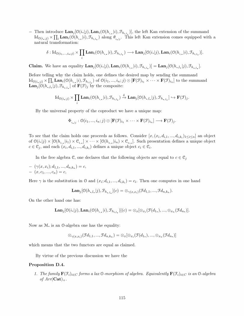
− Then introduce Lanj[O(i.|j),Lani(O(hi,. |i),Fhi,l. )], the left Kan extension of the summandIdO(i.;j)×

∏i Lani(O(hi,. |i),Fhi,l. ) along θ

i.|j . This left Kan extension comes equipped with anatural transformation:

δ : IdO(i1,...,in;j)×∏

i

Lani(O(hi,. |i),Fhi,l. ) −→ Lanj [O(i.|j),Lani(O(hi,. |i),Fhi,l. )].

Claim. We have an equality Lanj [O(i.|j),Lani(O(hi,. |i),Fhi,l. )] = Lanj[O(h.,l. |j),Fh.,l. ].

Before telling why the claim holds, one defines the desired map by sending the summandIdO(i.;j)×

∏i Lani(O(hi,. |i),Fhi,l. ) of O(i1, ..., in; j) ⊙ [F(F)i1 × · · · × F(F)in ] to the summand

Lanj[O(h.,l. |j),Fh.,l. ] of F(F)j by the composite:

IdO(i.;j)×∏

i

Lani(O(hi,. |i),Fhi,l. )δ−→ Lanj[O(h.,l. |j),Fh.,l. ] → F(F)j .

By the universal property of the coproduct we have a unique map:

Φi.|j : O(i1, ..., in; j)⊙ [F(F)i1 × · · · ×F(F)in ] −→ F(F)j .

To see that the claim holds one proceeds as follows. Consider [x, (xi, di,1, ..., di,ki)1≤i≤n] an objectof O(i.|j) × [O(h1,. |i1)× C1,. ]× · · · × [O(hn,. |in)× Cn,. ]. Such presentation defines a unique objectc ∈ Cj , and each (xi, di,1, ..., di,ki) defines a unique object ci ∈ Ci.

In the free algebra C, one declares that the following objects are equal to c ∈ Cj

− (γ(x, xi); d1,1, ..., dn,kn) = c,− (x, c1, ..., cn) = c,

Here γ is the substitution in O and (xi; di,1, ..., di,ki) = ci. Then one computes in one hand

Lanj [O(h.,l. |j),Fh.,l. ](c) = ⊗γ(x,xi)(Fd1,1, ...,Fdn,kn).

On the other hand one has:

Lanj[O(i.|j),Lani(O(hi,. |i),Fhi,l. )](c) = ⊗x[⊗xi(F(d1.), ...,⊗xn(Fdn.)].

Now as M. is an O-algebra one has the equality:

⊗γ(x,xi)(Fd1,1, ...,Fdn,kn) = ⊗x[⊗xi(F(d1.), ...,⊗xn(Fdn.)]

which means that the two functors are equal as claimed.

By virtue of the previous discussion we have the

Proposition D.4.

1. The family F(Fi)i∈C forms a lax O-morphism of algebra. Equivalently F(Fi)i∈C is an O-algebraof Arr(Cat)+.

115

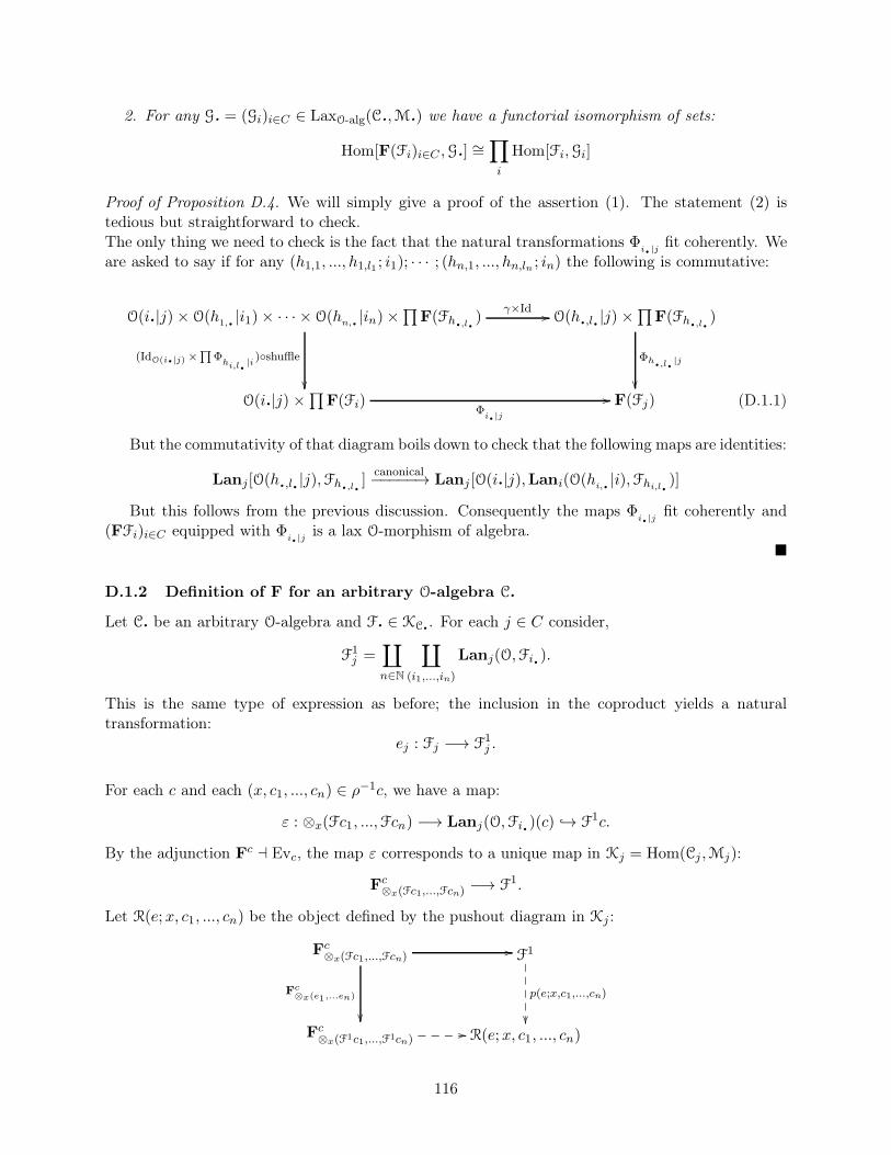
2. For any G. = (Gi)i∈C ∈ LaxO-alg(C.,M.) we have a functorial isomorphism of sets:

Hom[F(Fi)i∈C ,G.] ∼=∏

i

Hom[Fi,Gi]

Proof of Proposition D.4. We will simply give a proof of the assertion (1). The statement (2) istedious but straightforward to check.The only thing we need to check is the fact that the natural transformations Φ

i.|j fit coherently. Weare asked to say if for any (h1,1, ..., h1,l1 ; i1); · · · ; (hn,1, ..., hn,ln ; in) the following is commutative:

O(i.|j)× O(h1,. |i1)× · · · × O(hn,. |in)×∏

F(Fh.,l. ) O(h.,l. |j) ×∏

F(Fh.,l. )

O(i.|j) ×∏

F(Fi) F(Fj)

γ×Id //

Φi.|j

//

Φh.,l. |j

��

(IdO(i.|j) ×∏

Φhi,l. |i

)◦shuffle

��(D.1.1)

But the commutativity of that diagram boils down to check that the following maps are identities:

Lanj[O(h.,l. |j),Fh.,l. ]canonical−−−−−→ Lanj [O(i.|j),Lani(O(hi,. |i),Fhi,l. )]

But this follows from the previous discussion. Consequently the maps Φi.|j fit coherently and

(FFi)i∈C equipped with Φi.|j is a lax O-morphism of algebra.

�

D.1.2 Definition of F for an arbitrary O-algebra C.

Let C. be an arbitrary O-algebra and F. ∈ KC.. For each j ∈ C consider,

F1j =

∐

n∈N

∐

(i1,...,in)

Lanj(O,Fi.).

This is the same type of expression as before; the inclusion in the coproduct yields a naturaltransformation:

ej : Fj −→ F1j .

For each c and each (x, c1, ..., cn) ∈ ρ−1c, we have a map:

ε : ⊗x(Fc1, ...,Fcn) −→ Lanj(O,Fi.)(c) → F1c.

By the adjunction Fc ⊣ Evc, the map ε corresponds to a unique map in Kj = Hom(Cj ,Mj):

Fc⊗x(Fc1,...,Fcn)−→ F1.

Let R(e;x, c1, ..., cn) be the object defined by the pushout diagram in Kj :

Fc⊗x(Fc1,...,Fcn) F1

Fc⊗x(F1c1,...,F1cn) R(e;x, c1, ..., cn)

//

Fc⊗x(e1,...en)

��

p(e;x,c1,...,cn)

��✤✤✤✤✤

//❴❴❴❴

116

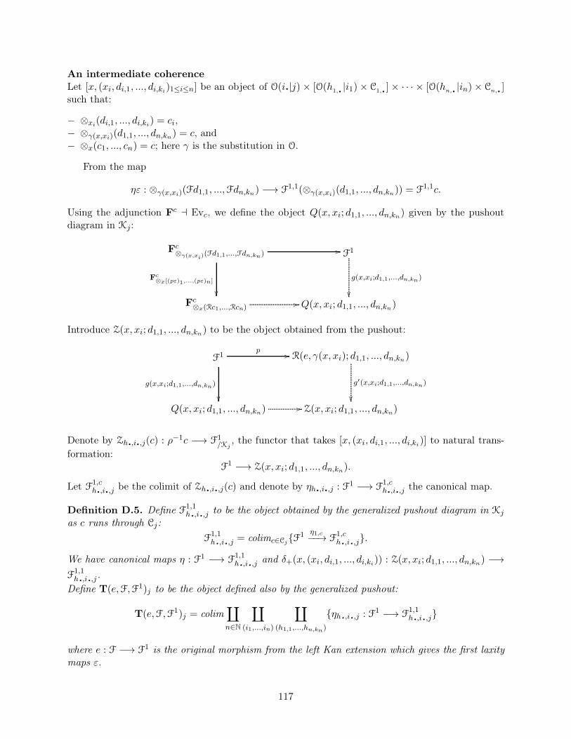
An intermediate coherenceLet [x, (xi, di,1, ..., di,ki)1≤i≤n] be an object of O(i.|j) × [O(h1,. |i1)× C1,. ]× · · · × [O(hn,. |in)× Cn,. ]such that:

− ⊗xi(di,1, ..., di,ki) = ci,− ⊗γ(x,xi)(d1,1, ..., dn,kn) = c, and− ⊗x(c1, ..., cn) = c; here γ is the substitution in O.

From the map

ηε : ⊗γ(x,xi)(Fd1,1, ...,Fdn,kn) −→ F1,1(⊗γ(x,xi)(d1,1, ..., dn,kn)) = F1,1c.

Using the adjunction Fc ⊣ Evc, we define the object Q(x, xi; d1,1, ..., dn,kn) given by the pushoutdiagram in Kj:

Fc⊗γ(x,xi)(Fd1,1,...,Fdn,kn) F1

Fc⊗x(Rc1,...,Rcn) Q(x, xi; d1,1, ..., dn,kn)

//

Fc⊗x[(pε)1,...,(pε)n]

��

g(x,xi;d1,1,...,dn,kn)

��//

Introduce Z(x, xi; d1,1, ..., dn,kn) to be the object obtained from the pushout:

F1 R(e, γ(x, xi); d1,1, ..., dn,kn)

Q(x, xi; d1,1, ..., dn,kn) Z(x, xi; d1,1, ..., dn,kn)

p //

g(x,xi;d1,1,...,dn,kn)

��

g′(x,xi;d1,1,...,dn,kn)

��//

Denote by Zh.,i.,j(c) : ρ−1c −→ F1/Kj

, the functor that takes [x, (xi, di,1, ..., di,ki)] to natural trans-

formation:F1 −→ Z(x, xi; d1,1, ..., dn,kn).

Let F1,ch.,i.,j be the colimit of Zh.,i.,j(c) and denote by ηh.,i.,j : F1 −→ F

1,ch.,i.,j the canonical map.

Definition D.5. Define F1,1h.,i.,j to be the object obtained by the generalized pushout diagram in Kj

as c runs through Cj:

F1,1h.,i.,j = colimc∈Cj

{F1 η1,c−−→ F

1,ch.,i.,j}.

We have canonical maps η : F1 −→ F1,1h.,i.,j and δ+(x, (xi, di,1, ..., di,ki)) : Z(x, xi; d1,1, ..., dn,kn) −→

F1,1h.,i.,j .

Define T(e,F,F1)j to be the object defined also by the generalized pushout:

T(e,F,F1)j = colim∐

n∈N

∐

(i1,...,in)

∐

(h1,1,...,hn,kn)

{ηh.,i.,j : F1 −→ F

1,1h.,i.,j}

where e : F −→ F1 is the original morphism from the left Kan extension which gives the first laxitymaps ε.

117

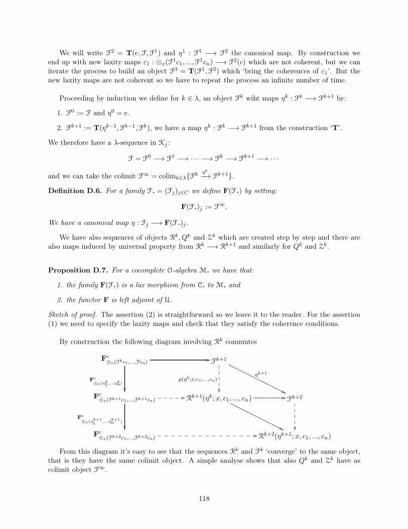
We will write F2 = T(e,F,F1) and η1 : F1 −→ F2 the canonical map. By construction weend up with new laxity maps ε1 : ⊗x(F

1c1, ...,F1cn) −→ F2(c) which are not coherent, but we can

iterate the process to build an object F3 = T(F1,F2) which ‘bring the coherences of ε1’. But thenew laxity maps are not coherent so we have to repeat the process an infinite number of time.

Proceeding by induction we define for k ∈ λ, an object Fk wiht maps ηk : Fk −→ Fk+1 by:

1. F0 := F and η0 = e.

2. Fk+1 := T(ηk−1,Fk−1,Fk), we have a map ηk : Fk −→ Fk+1 from the construction ‘T’.

We therefore have a λ-sequence in Kj:

F = F0 −→ F1 −→ · · · −→ Fk −→ Fk+1 −→ · · ·

and we can take the colimit F∞ = colimk∈λ{Fk ηk−→ Fk+1}.

Definition D.6. For a family F. = (Fj)j∈C we define F(F.) by setting:

F(F.)j := F∞.

We have a canonical map η : Fj −→ F(F.)j .

We have also sequences of objects Rk, Qk and Zk which are created step by step and there arealso maps induced by universal property from Rk −→ Rk+1 and similarly for Qk and Zk.

Proposition D.7. For a cocomplete O-algebra M. we have that:

1. the family F(F.) is a lax morphism from C. to M. and

2. the functor F is left adjoint of U.

Sketch of proof. The assertion (2) is straightforward so we leave it to the reader. For the assertion(1) we need to specify the laxity maps and check that they satisfy the coherence conditions.

By construction the following diagram involving Rk commutes

Fc⊗x(Fkc1,...,Fcn) Fk+1

Fc⊗x(Fk+1c1,...,Fk+1cn) Rk+1(ηk;x, c1, ..., cn) Fk+2

Fc⊗x(Fk+2c1,...,Fk+2cn) Rk+2(ηk+1;x, c1, ..., cn)

//

Fc

⊗x(ηk1 ,...ηkn)

��

p(ηk ;x,c1,...,cn)

��✤✤✤✤✤

//❴❴❴❴❴ //

Fc

⊗x(ηk+11 ,...ηk+1

n )

��//❴❴❴❴❴❴❴❴❴❴❴❴❴❴❴

��✤✤✤✤✤

''

ηk+1

''

From this diagram it’s easy to see that the sequences Rk and Fk ‘converge’ to the same object,that is they have the same colimit object. A simple analyse shows that also Qk and Zk have ascolimit object F∞.

118

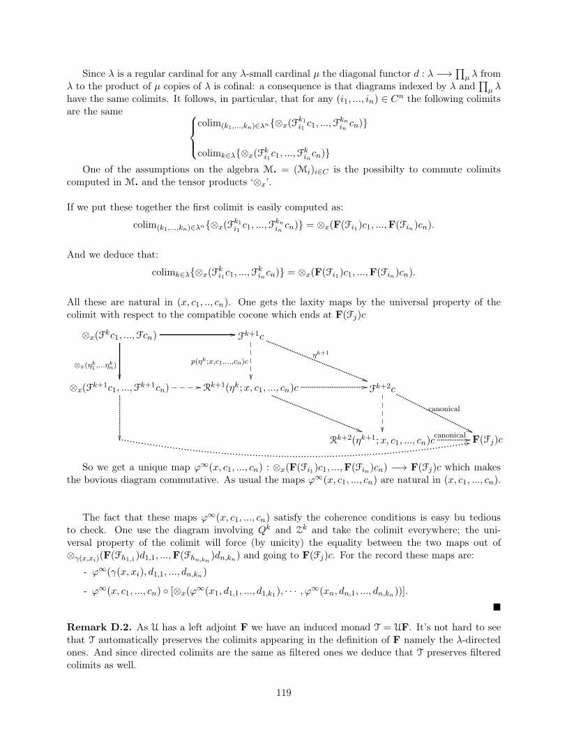
Since λ is a regular cardinal for any λ-small cardinal µ the diagonal functor d : λ −→∏µ λ from

λ to the product of µ copies of λ is cofinal: a consequence is that diagrams indexed by λ and∏µ λ

have the same colimits. It follows, in particular, that for any (i1, ..., in) ∈ Cn the following colimits

are the same

colim(k1,...,kn)∈λn{⊗x(Fk1i1c1, ...,F

knincn)}

colimk∈λ{⊗x(Fki1c1, ...,F

kincn)}

One of the assumptions on the algebra M. = (Mi)i∈C is the possibilty to commute colimitscomputed in M. and the tensor products ‘⊗x’.

If we put these together the first colimit is easily computed as:

colim(k1,...,kn)∈λn{⊗x(Fk1i1c1, ...,F

knincn)} = ⊗x(F(Fi1)c1, ...,F(Fin)cn).

And we deduce that:

colimk∈λ{⊗x(Fki1c1, ...,F

kincn)} = ⊗x(F(Fi1)c1, ...,F(Fin)cn).

All these are natural in (x, c1, .., cn). One gets the laxity maps by the universal property of thecolimit with respect to the compatible cocone which ends at F(Fj)c

⊗x(Fkc1, ...,Fcn) Fk+1c

⊗x(Fk+1c1, ...,Fk+1cn) Rk+1(ηk;x, c1, ..., cn)c Fk+2c

Rk+2(ηk+1;x, c1, ..., cn)c F(Fj)c

//

⊗x(ηk1 ,...ηkn)

��

p(ηk ;x,c1,...,cn)c

��✤✤✤✤✤

//❴❴❴❴ //

��✤✤✤✤✤

))

ηk+1

))

canonical

''canonical //�� 22

So we get a unique map ϕ∞(x, c1, ..., cn) : ⊗x(F(Fi1)c1, ...,F(Fin)cn) −→ F(Fj)c which makesthe bovious diagram commutative. As usual the maps ϕ∞(x, c1, ..., cn) are natural in (x, c1, ..., cn).

The fact that these maps ϕ∞(x, c1, ..., cn) satisfy the coherence conditions is easy bu tediousto check. One use the diagram involving Qk and Zk and take the colimit everywhere; the uni-versal property of the colimit will force (by unicity) the equality between the two maps out of⊗γ(x,xi)(F(Fh1,1)d1,1, ...,F(Fhn,kn

)dn,kn) and going to F(Fj)c. For the record these maps are:

- ϕ∞(γ(x, xi), d1,1, ..., dn,kn)

- ϕ∞(x, c1, ..., cn) ◦ [⊗x(ϕ∞(x1, d1,1, ..., d1,k1), · · · , ϕ

∞(xn, dn,1, ..., dn,kn))].

�

Remark D.2. As U has a left adjoint F we have an induced monad T = UF. It’s not hard to seethat T automatically preserves the colimits appearing in the definition of F namely the λ-directedones. And since directed colimits are the same as filtered ones we deduce that T preserves filteredcolimits as well.

119

D.2 LaxO-alg(C.,M.) is monadic over Hom(C.,M.)

Let σ1, σ2 : F. −→ G. be a pair of parallel morphisms between two lax-morphisms in LaxO-alg(C.,M.).Denote by L : G. −→ E. the coequalizer of σ1, σ2 in KC. =

∏i∈C Hom(Ci,Mi):

UF. UG. E.σ1

//σ2 // L //

Note that we’ve freely identified σi and it’s image Uσi. The following lemma is the general versionof lemma C.3 except that we do not use the language of precongruences.

Lemma D.8. Consider F.,G.,E. with σ1, σ2 and L as before. Assume that for every (x, c1, ..., cn) ∈O(i1, ..., in; j) × Ci1 × · · · × Cin with c = ⊗x(c1, ..., cn) and any l ∈ {1, ..., n} the following equalityholds:

Lc◦ϕG(x, c1, ..., cn)◦[⊗x(IdGc1 , ..., σ1(cl), ..., IdGcn)] = Lc◦ϕG

(x, c1, ..., cn)◦[⊗x(IdGc1 , ..., σ2(cl), ..., IdGcn)].

Then we have:

1. E. becomes a lax morphism and

2. L is the coequalizer of σ1 , σ2 in LaxO-alg(C.,M.).

When there is no confusion we will simply write ϕG

instead of ϕG(x, c1, ..., cn).

Sketch of proof. The assertion (2) will follow from the proof of (1). To prove (1) we will simply givethe laxity maps; the coherence conditions are straightforward.

As mentioned before, the assumptions on M. allow to distribute (factor wise) colimits over eachtensor product ⊗x. It follows that ⊗x(Ec1, ...Ecn) equipped with the maps ⊗x(Lc1 , ..., Lcn) is thecolimit of the diagram

ǫ(σ1, σ2; c1, ..., cn) =∐

(τ1,...,τn)∈{1,2}n

{⊗x(στ1c1, ..., στncn) : ⊗x(Fc1, ...,Fcn) −→ ⊗x(Gc1, ...,Gcn)}.

(For each l, στl is either σ1 or σ2).

For each (τ1, ..., τn) ∈ {1, 2}n let Θ(τ1, ..., τn) = Lc ◦ϕG

(x, c1, ..., cn) ◦⊗x(στ1c1, ..., στncn) be themap illustrated in the diagram below:

⊗x(Fc1, ...,Fcn) Fc

⊗x(Gc1, ...,Gcn) GcϕG

//

⊗x(στ1 c1,...,στncn)

��

Ec

Lc

��

Now we claim that Θ(τ1, ..., τn) = Θ(τ ′1, ..., τ′n) for all (τ1, ..., τn) , (τ ′1, ..., τ

′n) in {1, 2}n. The

claim will holds as soon as we show that for every l ∈ {1, ..., n} we have Θ(τ1, ..., τl, ...τn) =Θ(τ1, ..., τ

′l , ..., τn) where τl and τ ′l are ‘conjugate’ that is: if τl = 1 then τ ′l = 2 and vice versa.

Let’s assume that τl = 1 (hence τ ′l = 2) that is στl = σ1.We establish successively the following equalities:

120

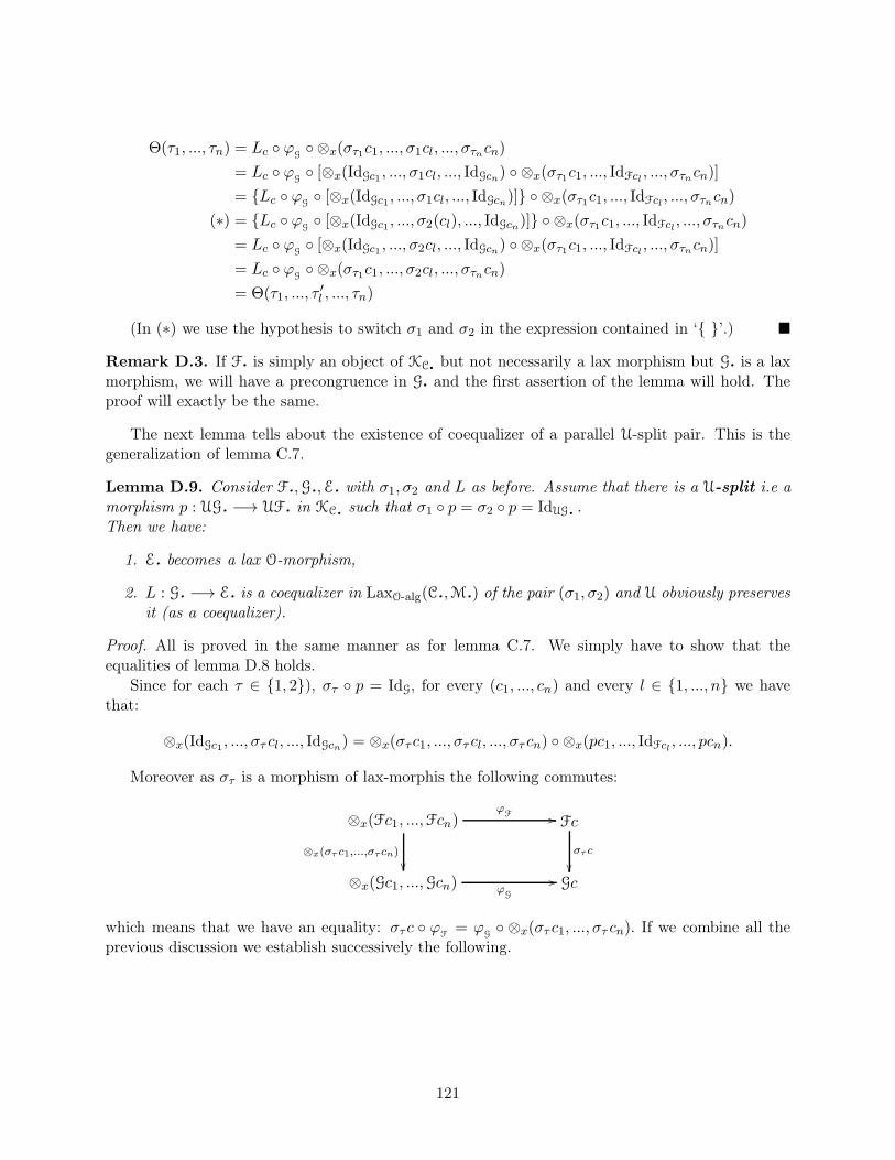
Θ(τ1, ..., τn) = Lc ◦ ϕG◦ ⊗x(στ1c1, ..., σ1cl, ..., στncn)

= Lc ◦ ϕG◦ [⊗x(IdGc1 , ..., σ1cl, ..., IdGcn) ◦ ⊗x(στ1c1, ..., IdFcl , ..., στncn)]

= {Lc ◦ ϕG◦ [⊗x(IdGc1 , ..., σ1cl, ..., IdGcn)]} ◦ ⊗x(στ1c1, ..., IdFcl , ..., στncn)

(∗) = {Lc ◦ ϕG◦ [⊗x(IdGc1 , ..., σ2(cl), ..., IdGcn)]} ◦ ⊗x(στ1c1, ..., IdFcl , ..., στncn)

= Lc ◦ ϕG◦ [⊗x(IdGc1 , ..., σ2cl, ..., IdGcn) ◦ ⊗x(στ1c1, ..., IdFcl , ..., στncn)]

= Lc ◦ ϕG◦ ⊗x(στ1c1, ..., σ2cl, ..., στncn)

= Θ(τ1, ..., τ′l , ..., τn)

(In (∗) we use the hypothesis to switch σ1 and σ2 in the expression contained in ‘{ }’.) �

Remark D.3. If F. is simply an object of KC. but not necessarily a lax morphism but G. is a laxmorphism, we will have a precongruence in G. and the first assertion of the lemma will hold. Theproof will exactly be the same.

The next lemma tells about the existence of coequalizer of a parallel U-split pair. This is thegeneralization of lemma C.7.

Lemma D.9. Consider F.,G.,E. with σ1, σ2 and L as before. Assume that there is a U-split i.e amorphism p : UG. −→ UF. in KC. such that σ1 ◦ p = σ2 ◦ p = IdUG. .Then we have:

1. E. becomes a lax O-morphism,

2. L : G. −→ E. is a coequalizer in LaxO-alg(C.,M.) of the pair (σ1, σ2) and U obviously preservesit (as a coequalizer).

Proof. All is proved in the same manner as for lemma C.7. We simply have to show that theequalities of lemma D.8 holds.

Since for each τ ∈ {1, 2}), στ ◦ p = IdG, for every (c1, ..., cn) and every l ∈ {1, ..., n} we havethat:

⊗x(IdGc1 , ..., στ cl, ..., IdGcn) = ⊗x(στc1, ..., στ cl, ..., στ cn) ◦ ⊗x(pc1, ..., IdFcl , ..., pcn).

Moreover as στ is a morphism of lax-morphis the following commutes:

⊗x(Fc1, ...,Fcn) Fc

⊗x(Gc1, ...,Gcn) Gc

ϕF //

ϕG

//

στ c

��⊗x(στ c1,...,στcn)

��

which means that we have an equality: στc ◦ ϕF= ϕ

G◦ ⊗x(στ c1, ..., στ cn). If we combine all the

previous discussion we establish successively the following.

121

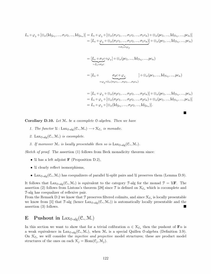
Lc ◦ ϕG◦ [⊗x(IdGc1 , ..., σ1cl, ..., IdGcn)] = Lc ◦ ϕG

◦ [⊗x(σ1c1, ..., σ1cl, ..., σ1cn) ◦ ⊗x(pc1, ..., IdFcl , ..., pcn)]

= [Lc ◦ ϕG◦ ⊗x(σ1c1, ..., σ1cl, ..., σ1cn)︸ ︷︷ ︸

=σ1c◦ϕF

] ◦ ⊗x(pc1, ..., IdFcl , ..., pcn)

= [Lc ◦ σ1c︸ ︷︷ ︸=Lc◦σ2c

◦ϕF] ◦ ⊗x(pc1, ..., IdFcl , ..., pcn)

= [Lc ◦ σ2c ◦ ϕF︸ ︷︷ ︸=ϕ

G◦⊗x(σ2c1,...,σ2cl,...,σ2cn)

] ◦ ⊗x(pc1, ..., IdFcl, ..., pcn)

= [Lc ◦ ϕG◦ ⊗x(σ2c1, ..., σ2cl, ..., σ2cn)] ◦ ⊗x(pc1, ..., IdFcl , ..., pcn)

= Lc ◦ ϕG◦ [⊗x(σ2c1, ..., σ2cl, ..., σ2cn) ◦ ⊗x(pc1, ..., IdFcl , ..., pcn)]

= Lc ◦ ϕG◦ [⊗x(IdGc1 , ..., σ2cl, ..., IdGcn)].

�

Corollary D.10. Let M. be a cocomplete O-algebra. Then we have

1. The functor U : LaxO-alg(C.,M.) −→ KC. is monadic.

2. LaxO-alg(C.,M.) is cocomplete.

3. If moreover M. is locally presentable then so is LaxO-alg(C.,M.).

Sketch of proof. The assertion (1) follows from Beck monadicity theorem since:

• U has a left adjoint F (Proposition D.2),

• U clearly reflect isomorphisms,

• LaxO-alg(C.,M.) has coequalizers of parallel U-split pairs and U preserves them (Lemma D.9).

It follows that LaxO-alg(C.,M.) is equivalent to the category T-alg for the monad T = UF. Theassertion (2) follows from Lintons’s theorem [28] since T is defined on KC. which is cocomplete andT-alg has coequalizer of reflexive pair.From the Remark D.2 we know that T preserves filtered colimits, and since KC. is locally presentablewe know from [1] that T-alg (hence LaxO-alg(C.,M.)) is automatically locally presentable and theassertion (3) follows. �

E Pushout in LaxO-alg(C.,M.)

In this section we want to show that for a trivial cofibration α ∈ KC. then the pushout of Fα isa weak equivalence in LaxO-alg(C.,M.), when M. is a special Quillen O-algebra (Definition 3.9).On KC. we will consider the injective and projective model structures; these are product modelstructures of the ones on each Kj = Hom(Cj,Mj).

122

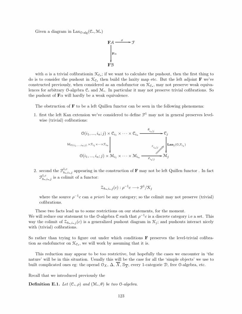
Given a diagram in LaxO-alg(C.,M.)

FA F

FB

σ //

Fα

��

with α is a trivial cofibrationin KC.; if we want to calculate the pushout, then the first thing todo is to consider the pushout in KC. then build the laxity map etc. But the left adjoint F we’veconstructed previously, when considered as an endofunctor on KC., may not preserve weak equiva-lences for arbitrary O-algebra C. and M.. In particular it may not preserve trivial cofibrations. Sothe pushout of Fα will hardly be a weak equivalence.

The obstruction of F to be a left Quillen functor can be seen in the following phenomena:

1. first the left Kan extension we’ve considered to define F1 may not in general preserves level-wise (trivial) cofibrations:

O(i1, ..., in; j)× Ci1 × · · · × Cin Cj

O(i1, ..., in; j) ×Mi1 × · · · ×Min Mj

θi.|j //

ρi.|j

//

Lanj(O,Fi. )

��

IdO(i1,...,in;j) ×Fi1×···×Fin

��

εi.|j

;C⑧⑧⑧⑧⑧⑧

⑧⑧⑧⑧⑧⑧

2. second the F1,ch.,i.,j appearing in the construction of F may not be left Quillen functor . In fact

F1,ch.,i.,j is a colimit of a functor:

Zh.,i.,j(c) : ρ−1c −→ F1/Kj

where the source ρ−1c can a priori be any category; so the colimit may not preserve (trivial)cofibrations.

These two facts lead us to some restrictions on our statements, for the moment.We will reduce our statement to the O-algebra C such that ρ−1c is a discrete category i.e a set. Thisway the colimit of Zh.,i.,j(c) is a generalized pushout diagram in Kj; and pushouts interact nicelywith (trivial) cofibrations.

So rather than trying to figure out under which conditions F preserves the level-trivial cofibra-tion as endofunctor on KC., we will work by assuming that it is.

This reduction may appear to be too restrictive, but hopefully the cases we encounter in ‘thenature’ will be in this situation. Usually this will be the case for all the ‘simple objects’ we use tobuilt complicated ones eg: the operad OX , ∆, X, SX , every 1-categorie D, free O-algebra, etc.

Recall that we introduced previously the

Definition E.1. Let (C., ρ) and (M., θ) be two O-algebra.

123

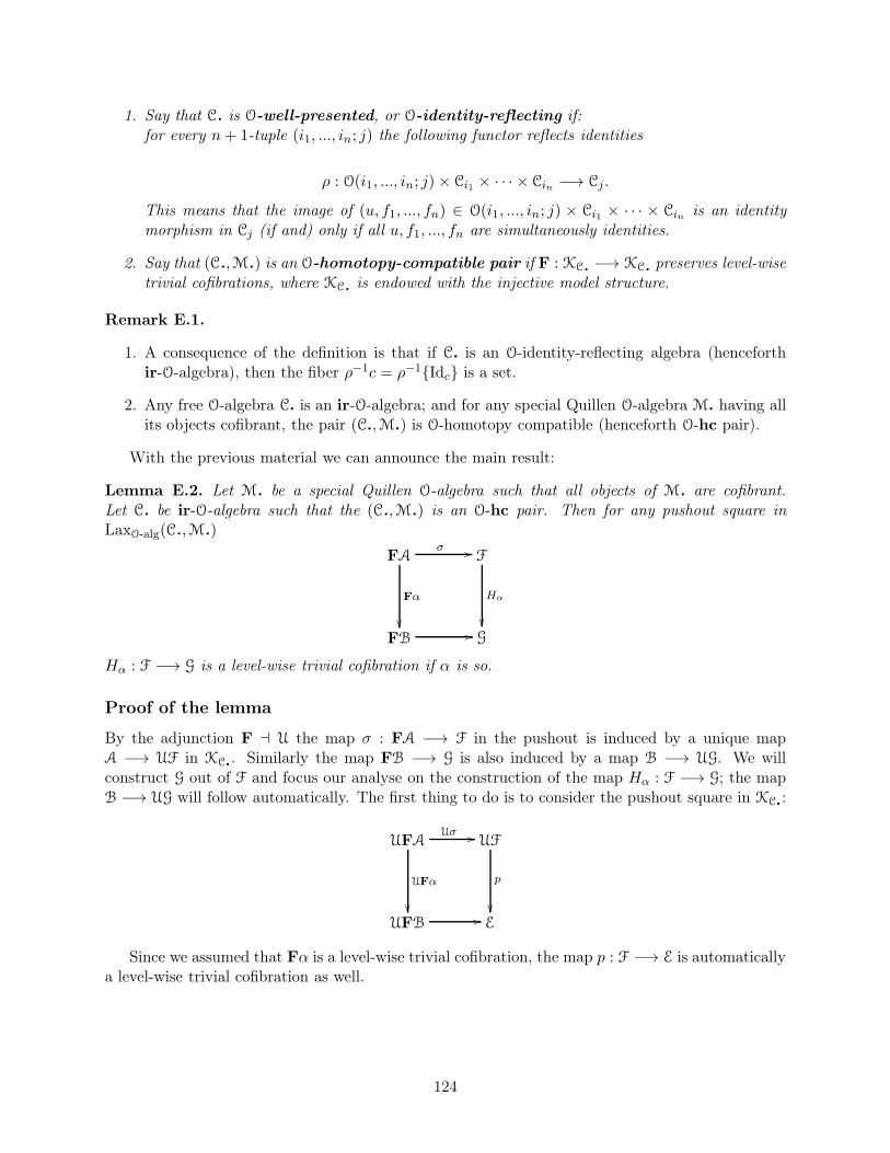
1. Say that C. is O-well-presented, or O-identity-reflecting if:for every n+ 1-tuple (i1, ..., in; j) the following functor reflects identities

ρ : O(i1, ..., in; j)× Ci1 × · · · × Cin −→ Cj .

This means that the image of (u, f1, ..., fn) ∈ O(i1, ..., in; j) × Ci1 × · · · × Cin is an identitymorphism in Cj (if and) only if all u, f1, ..., fn are simultaneously identities.

2. Say that (C.,M.) is an O-homotopy-compatible pair if F : KC. −→ KC. preserves level-wisetrivial cofibrations, where KC. is endowed with the injective model structure.

Remark E.1.

1. A consequence of the definition is that if C. is an O-identity-reflecting algebra (henceforthir-O-algebra), then the fiber ρ−1c = ρ−1{Idc} is a set.

2. Any free O-algebra C. is an ir-O-algebra; and for any special Quillen O-algebra M. having allits objects cofibrant, the pair (C.,M.) is O-homotopy compatible (henceforth O-hc pair).

With the previous material we can announce the main result:

Lemma E.2. Let M. be a special Quillen O-algebra such that all objects of M. are cofibrant.Let C. be ir-O-algebra such that the (C.,M.) is an O-hc pair. Then for any pushout square inLaxO-alg(C.,M.)

FA F

FB G

σ //

Fα

��

Hα

��//

Hα : F −→ G is a level-wise trivial cofibration if α is so.

Proof of the lemma

By the adjunction F ⊣ U the map σ : FA −→ F in the pushout is induced by a unique mapA −→ UF in KC.. Similarly the map FB −→ G is also induced by a map B −→ UG. We willconstruct G out of F and focus our analyse on the construction of the map Hα : F −→ G; the mapB −→ UG will follow automatically. The first thing to do is to consider the pushout square in KC.:

UFA UF

UFB E

Uσ //

UFα

��

p

��//

Since we assumed that Fα is a level-wise trivial cofibration, the map p : F −→ E is automaticallya level-wise trivial cofibration as well.

124

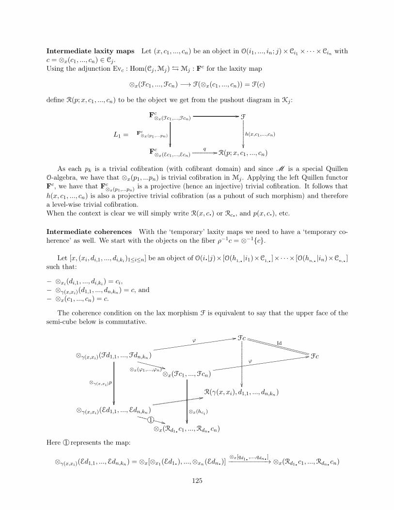
Intermediate laxity maps Let (x, c1, ..., cn) be an object in O(i1, ..., in; j)×Ci1 × · · · ×Cin withc = ⊗x(c1, ..., cn) ∈ Cj.Using the adjunction Evc : Hom(Cj ,Mj)⇆Mj : F

c for the laxity map

⊗x(Fc1, ...,Fcn) −→ F(⊗x(c1, ..., cn)) = F(c)

define R(p;x, c1, ..., cn) to be the object we get from the pushout diagram in Kj:

L1 =

Fc⊗x(Fc1,...,Fcn) F

Fc⊗x(Ec1,...,Ecn) R(p;x, c1, ..., cn)

//

Fc⊗x(p1,...pn)

��

h(x,c1,...,cn)

��q //

As each pk is a trivial cofibration (with cofibrant domain) and since M is a special QuillenO-algebra, we have that ⊗x(p1, ...pn) is trivial cofibration in Mj . Applying the left Quillen functorFc, we have that Fc⊗x(p1,...pn)

is a projective (hence an injective) trivial cofibration. It follows that

h(x, c1, ..., cn) is also a projective trivial cofibration (as a puhout of such morphism) and thereforea level-wise trivial cofibration.When the context is clear we will simply write R(x, c.) or Rc., and p(x, c.), etc.

Intermediate coherences With the ‘temporary’ laxity maps we need to have a ‘temporary co-herence’ as well. We start with the objects on the fiber ρ−1c = ⊗−1{c}.

Let [x, (xi, di,1, ..., di,ki)1≤i≤n] be an object of O(i.|j)× [O(h1,. |i1)×C1,. ]×· · ·× [O(hn,. |in)×Cn,. ]such that:

− ⊗xi(di,1, ..., di,ki) = ci,− ⊗γ(x,xi)(d1,1, ..., dn,kn) = c, and− ⊗x(c1, ..., cn) = c.

The coherence condition on the lax morphism F is equivalent to say that the upper face of thesemi-cube below is commutative.

⊗γ(x,xi)(Fd1,1, ...,Fdn,kn )

Fc

⊗x(Fc1, ...,Fcn)

Fc

ϕ11❞❞❞❞❞❞❞❞❞❞❞❞❞❞❞❞❞❞❞❞❞❞❞❞❞❞

⊗x(ϕ1,...,ϕn)++❲❲❲❲

❲❲❲❲❲

Id

❲❲❲❲❲❲❲❲

❲❲❲❲❲❲❲❲

❲❲❲❲

❲❲❲❲❲❲❲❲

❲❲❲❲❲❲❲❲

❲❲❲❲

ϕ11❞❞❞❞❞❞❞❞❞❞❞❞❞❞❞❞❞❞❞❞❞❞❞❞❞❞❞❞❞❞❞

⊗γ(x,xi)(Ed1,1, ...,Edn,kn)

R(γ(x, xi), d1,1, ..., dn,kn)

⊗x(Rd1.c1, ...,Rdn.cn)

11

⊗γ(x,xi)p

��⊗x(hci )

��

��

1❲❲❲❲

++❲❲❲❲

Here 1 represents the map:

⊗γ(x,xi)(Ed1,1, ...,Edn,kn) = ⊗x[⊗x1(Ed1.), ...,⊗xn(Edn.)]⊗x[qd1. ,...,qdn. ]−−−−−−−−−−→ ⊗x(Rd1.c1, ...,Rdn.cn)

125

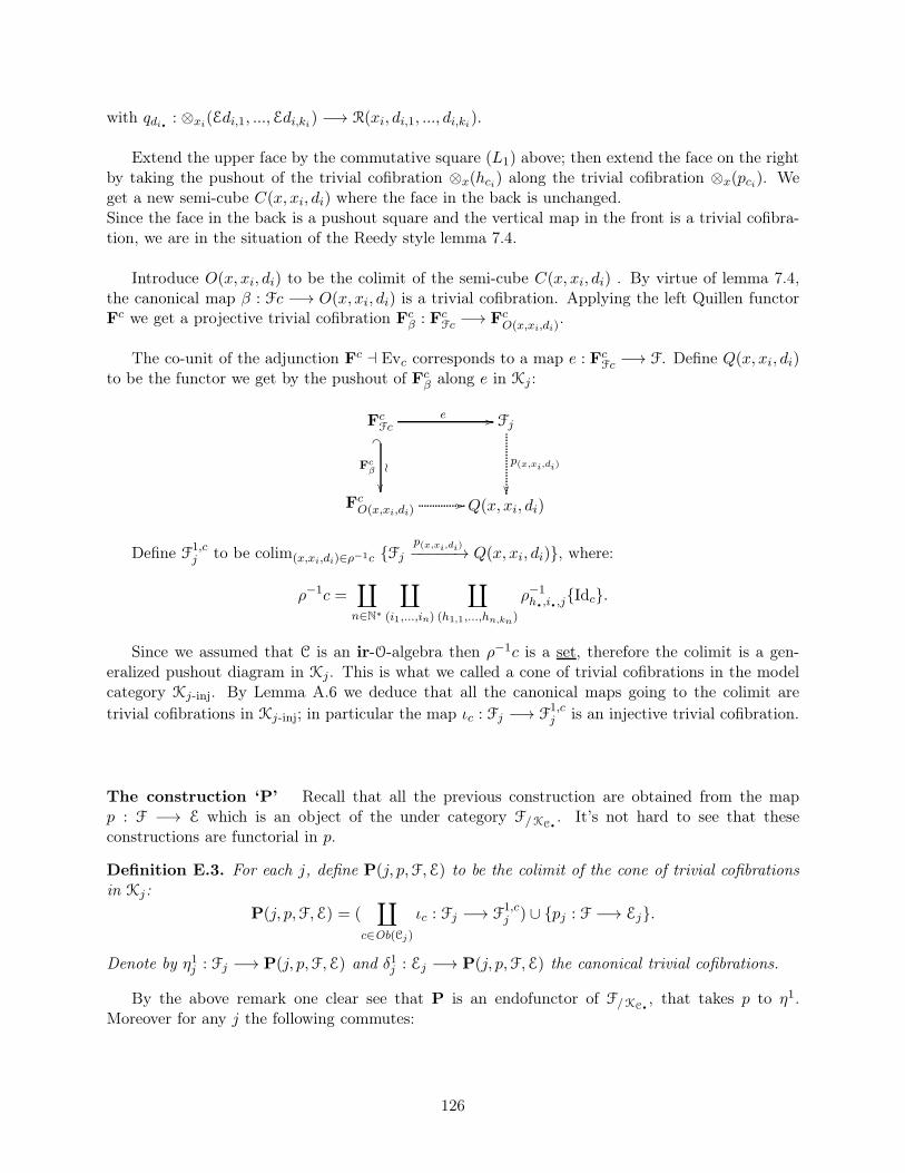
with qdi. : ⊗xi(Edi,1, ...,Edi,ki) −→ R(xi, di,1, ..., di,ki).

Extend the upper face by the commutative square (L1) above; then extend the face on the rightby taking the pushout of the trivial cofibration ⊗x(hci) along the trivial cofibration ⊗x(pci). Weget a new semi-cube C(x, xi, di) where the face in the back is unchanged.Since the face in the back is a pushout square and the vertical map in the front is a trivial cofibra-tion, we are in the situation of the Reedy style lemma 7.4.

Introduce O(x, xi, di) to be the colimit of the semi-cube C(x, xi, di) . By virtue of lemma 7.4,the canonical map β : Fc −→ O(x, xi, di) is a trivial cofibration. Applying the left Quillen functorFc we get a projective trivial cofibration Fcβ : Fc

Fc −→ FcO(x,xi,di).

The co-unit of the adjunction Fc ⊣ Evc corresponds to a map e : FcFc −→ F. Define Q(x, xi, di)to be the functor we get by the pushout of Fcβ along e in Kj :

FcFc Fj

FcO(x,xi,di) Q(x, xi, di)

e //

_�

Fcβ ≀

��

p(x,xi,di)

��//

Define F1,cj to be colim(x,xi,di)∈ρ−1c {Fj

p(x,xi,di)−−−−−→ Q(x, xi, di)}, where:

ρ−1c =∐

n∈N∗

∐

(i1,...,in)

∐

(h1,1,...,hn,kn)

ρ−1h.,i.,j{Idc}.

Since we assumed that C is an ir-O-algebra then ρ−1c is a set, therefore the colimit is a gen-eralized pushout diagram in Kj. This is what we called a cone of trivial cofibrations in the modelcategory Kj-inj. By Lemma A.6 we deduce that all the canonical maps going to the colimit are

trivial cofibrations in Kj-inj; in particular the map ιc : Fj −→ F1,cj is an injective trivial cofibration.

The construction ‘P’ Recall that all the previous construction are obtained from the mapp : F −→ E which is an object of the under category F/KC. . It’s not hard to see that theseconstructions are functorial in p.

Definition E.3. For each j, define P(j, p,F,E) to be the colimit of the cone of trivial cofibrationsin Kj:

P(j, p,F,E) = (∐

c∈Ob(Cj)

ιc : Fj −→ F1,cj ) ∪ {pj : F −→ Ej}.

Denote by η1j : Fj −→ P(j, p,F,E) and δ1j : Ej −→ P(j, p,F,E) the canonical trivial cofibrations.

By the above remark one clear see that P is an endofunctor of F/KC. , that takes p to η1.Moreover for any j the following commutes:

126

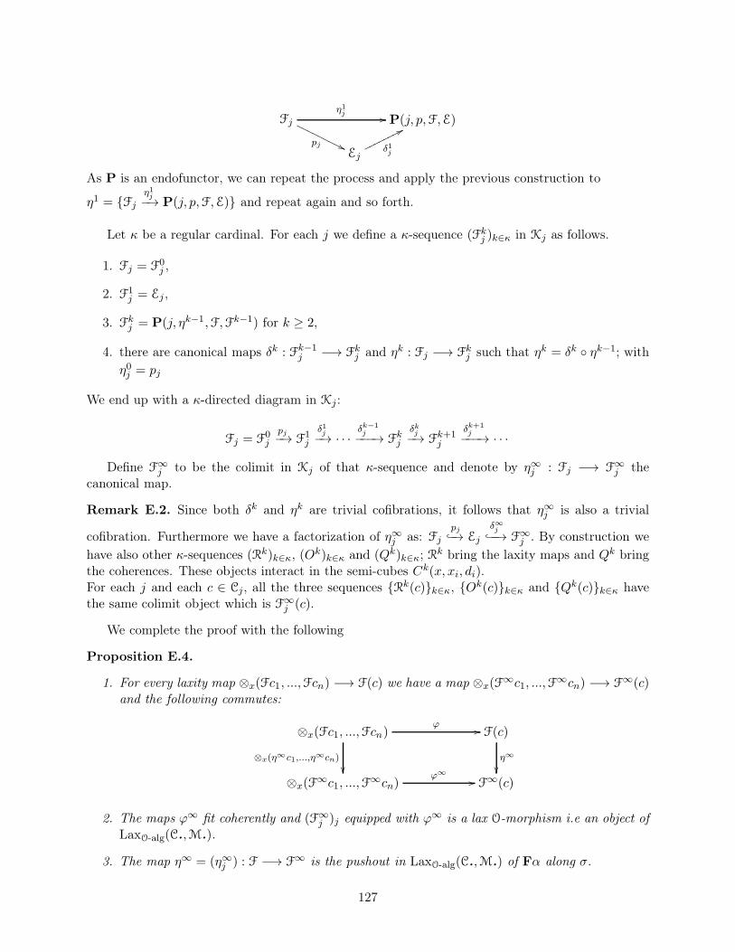
Fj P(j, p,F,E)

Ej

η1j //

pj ''❖❖❖❖

❖❖❖❖❖

δ1j

77♦♦♦♦♦♦♦♦

As P is an endofunctor, we can repeat the process and apply the previous construction to

η1 = {Fjη1j−→ P(j, p,F,E)} and repeat again and so forth.

Let κ be a regular cardinal. For each j we define a κ-sequence (Fkj )k∈κ in Kj as follows.

1. Fj = F0j ,

2. F1j = Ej ,

3. Fkj = P(j, ηk−1,F,Fk−1) for k ≥ 2,

4. there are canonical maps δk : Fk−1j −→ Fkj and ηk : Fj −→ Fkj such that ηk = δk ◦ ηk−1; with

η0j = pj

We end up with a κ-directed diagram in Kj :

Fj = F0j

pj−→ F1

j

δ1j−→ · · ·

δk−1j−−−→ Fkj

δkj−→ Fk+1

j

δk+1j−−−→ · · ·

Define F∞j to be the colimit in Kj of that κ-sequence and denote by η∞j : Fj −→ F∞

j thecanonical map.

Remark E.2. Since both δk and ηk are trivial cofibrations, it follows that η∞j is also a trivial

cofibration. Furthermore we have a factorization of η∞j as: Fjpj−→ Ej

δ∞j−−→ F∞

j . By construction we

have also other κ-sequences (Rk)k∈κ, (Ok)k∈κ and (Qk)k∈κ; R

k bring the laxity maps and Qk bringthe coherences. These objects interact in the semi-cubes Ck(x, xi, di).For each j and each c ∈ Cj, all the three sequences {Rk(c)}k∈κ, {O

k(c)}k∈κ and {Qk(c)}k∈κ havethe same colimit object which is F∞

j (c).

We complete the proof with the following

Proposition E.4.

1. For every laxity map ⊗x(Fc1, ...,Fcn) −→ F(c) we have a map ⊗x(F∞c1, ...,F

∞cn) −→ F∞(c)and the following commutes:

⊗x(Fc1, ...,Fcn) F(c)

⊗x(F∞c1, ...,F

∞cn) F∞(c)

ϕ //

⊗x(η∞c1,...,η∞cn)

��η∞

��ϕ∞//

2. The maps ϕ∞ fit coherently and (F∞j )j equipped with ϕ∞ is a lax O-morphism i.e an object of

LaxO-alg(C.,M.).

3. The map η∞ = (η∞j ) : F −→ F∞ is the pushout in LaxO-alg(C.,M.) of Fα along σ.

127

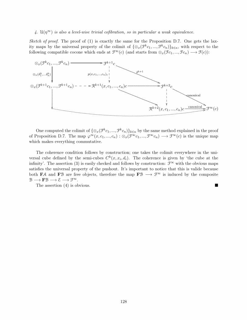
4. U(η∞) is also a level-wise trivial cofibration, so in particular a weak equivalence.

Sketch of proof. The proof of (1) is exactly the same for the Proposition D.7. One gets the lax-ity maps by the universal property of the colimit of {⊗x(F

kc1, ...,Fkcn)}k∈κ, with respect to the

following compatible cocone which ends at F∞(c) (and starts from ⊗x(Fc1, ...,Fcn) −→ F(c)):

⊗x(Fkc1, ...,F

kcn) Fk+1c

⊗x(Fk+1c1, ...,Fk+1cn) Rk+1(x, c1, ..., cn)c Fk+2c

Rk+2(x, c1, ..., cn)c F∞(c)

//

⊗x(δk1 ,...δkn)

��

p(x,c1,...,cn)c

��✤✤✤✤✤

//❴❴❴❴ //

��✤✤✤✤✤

))

δk+1

))

canonical

''canonical //�� 22

One computed the colimit of {⊗x(Fkc1, ...,F

kcn)}k∈κ by the same method explained in the proofof Proposition D.7. The map ϕ∞(x, c1, ..., cn) : ⊗x(F

∞c1, ...,F∞cn) −→ F∞(c) is the unique map

which makes everything commutative.

The coherence condition follows by construction; one takes the colimit everywhere in the uni-versal cube defined by the semi-cubes Ck(x, xi, di). The coherence is given by ‘the cube at theinfinity’. The assertion (3) is easily checked and follows by construction: F∞ with the obvious mapssatisfies the universal property of the pushout. It’s important to notice that this is valide becauseboth FA and FB are free objects, therefore the map FB −→ F∞ is induced by the compositeB −→ FB −→ E −→ F∞.

The assertion (4) is obvious. �

128

References

[1] Jiří Adámek and Jiří Rosický. Locally presentable and accessible categories, volume 189 ofLondon Mathematical Society Lecture Note Series. Cambridge University Press, Cambridge,1994.

[2] Vigleik Angeltveit. Enriched Reedy categories. Proc. Amer. Math. Soc., 136(7):2323–2332,2008.

[3] H. V. Bacard. Segal Enriched Categories I. http://arxiv.org/abs/1009.3673.

[4] Clark Barwick. On left and right model categories and left and right Bousfield localizations.Homology, Homotopy Appl., 12(2):245–320, 2010.

[5] Jean Bénabou. Introduction to bicategories. In Reports of the Midwest Category Seminar,pages 1–77. Springer, Berlin, 1967.

[6] C. Berger and I. Moerdijk. On an extension of the notion of Reedy category.http://arxiv.org/abs/0809.3341.

[7] C. Berger and I. Moerdijk. On the homotopy theory of enriched categories.http://arxiv.org/abs/1201.2134.

[8] Clemens Berger and Ieke Moerdijk. Resolution of coloured operads and rectification of ho-motopy algebras. In Categories in algebra, geometry and mathematical physics, volume 431 ofContemp. Math., pages 31–58. Amer. Math. Soc., Providence, RI, 2007.

[9] F. Bonnin. Les groupements. http://arxiv.org/abs/math/0404233.

[10] Denis-Charles Cisinski. Les préfaisceaux comme modèles des types d’homotopie. Astérisque,(308):xxiv+390, 2006.

[11] Denis-Charles Cisinski. Catégories dérivables. Bulletin de la société mathématique de France,138(3):317–393, 2010.

[12] W. G. Dwyer and D. M. Kan. Function complexes in homotopical algebra. Topology, 19(4):427–440, 1980.

[13] W. G. Dwyer and J. Spaliński. Homotopy theories and model categories. In Handbook ofalgebraic topology, pages 73–126. North-Holland, Amsterdam, 1995.

[14] William G. Dwyer, Philip S. Hirschhorn, Daniel M. Kan, and Jeffrey H. Smith. Homotopy limitfunctors on model categories and homotopical categories, volume 113 of Mathematical Surveysand Monographs. American Mathematical Society, Providence, RI, 2004.

[15] Kenji Fukaya, Yong-Geun Oh, Hiroshi Ohta, and Kaoru Ono. Lagrangian intersection Floertheory: anomaly and obstruction. Part I, volume 46 of AMS/IP Studies in Advanced Mathe-matics. American Mathematical Society, Providence, RI, 2009.

[16] Kenji Fukaya, Yong-Geun Oh, Hiroshi Ohta, and Kaoru Ono. Lagrangian intersection Floertheory: anomaly and obstruction. Part II, volume 46 of AMS/IP Studies in Advanced Mathe-matics. American Mathematical Society, Providence, RI, 2009.

129

[17] Philip S. Hirschhorn. Model categories and their localizations, volume 99 of MathematicalSurveys and Monographs. American Mathematical Society, Providence, RI, 2003.

[18] Mark Hovey. Model categories, volume 63 of Mathematical Surveys and Monographs. AmericanMathematical Society, Providence, RI, 1999.

[19] Bart Jacobs. Categorical logic and type theory, volume 141 of Studies in Logic and the Foun-dations of Mathematics. North-Holland Publishing Co., Amsterdam, 1999.

[20] G. M. Kelly. Basic concepts of enriched category theory. Repr. Theory Appl. Categ.,(10):vi+137, 2005. Reprint of the 1982 original [Cambridge Univ. Press, Cambridge;MR0651714].

[21] G. M. Kelly and Stephen Lack. V -Cat is locally presentable or locally bounded if V is so.Theory Appl. Categ., 8:555–575, 2001.

[22] M. Kontsevich and Y. Soibelman. Notes on A-infinity algebras, A-infinity categories and non-commutative geometry. I. June 2006. http://arxiv.org/abs/math/0606241.

[23] Igor Kříž and J. P. May. Operads, algebras, modules and motives. Astérisque, (233):iv+145pp,1995.

[24] Stephen Lack. Icons. Appl. Categ. Structures, 18(3):289–307, 2010.

[25] T. Leinster. Basic Bicategories. http://arxiv.org/abs/math/9810017.

[26] T. Leinster. Up-to-Homotopy Monoids. http://arxiv.org/abs/math/9912084.

[27] Tom Leinster. Higher operads, higher categories, volume 298 of London Mathematical SocietyLecture Note Series. Cambridge University Press, Cambridge, 2004.

[28] F. E. J. Linton. Coequalizers in categories of algebras. In Sem. on Triples and CategoricalHomology Theory (ETH, Zürich, 1966/67), pages 75–90. Springer, Berlin, 1969.

[29] Jacob Lurie. Higher topos theory, volume 170 of Annals of Mathematics Studies. PrincetonUniversity Press, Princeton, NJ, 2009.

[30] Volodymyr Lyubashenko. Category of A∞-categories. Homology Homotopy Appl., 5(1):1–48,2003.

[31] Saunders Mac Lane. Categories for the working mathematician, volume 5 of Graduate Texts inMathematics. Springer-Verlag, New York, second edition, 1998.

[32] Daniel G. Quillen. Homotopical algebra. Lecture Notes in Mathematics, No. 43. Springer-Verlag,Berlin, 1967.

[33] Agustí Roig. Model category structures in bifibred categories. J. Pure Appl. Algebra, 95(2):203–223, 1994.

[34] Stefan Schwede and Brooke E. Shipley. Algebras and modules in monoidal model categories.Proc. London Math. Soc. (3), 80(2):491–511, 2000.

[35] Carlos Simpson. Homotopy theory of higher categories, volume 19 of New Mathematical Mono-graphs. Cambridge University Press, Cambridge, 2012.

130

[36] J. Smith. Combinatorial model categories. Unpublished.

[37] Alexandru Stanculescu. Bifibrations and weak factorisation systems. Applied Categorical Struc-tures.

[38] Ross Street. Enriched categories and cohomology. Repr. Theory Appl. Categ., (14):1–18, 2005.Reprinted from Quaestiones Math. 6 (1983), no. 1-3, 265–283 [MR0700252], with new com-mentary by the author.

[39] Harvey Wolff. V -cat and V -graph. J. Pure Appl. Algebra, 4:123–135, 1974.

131