Department of Economics Issn 1441-5429

Discussion paper 23/10

Human Capital Composition, Proximity to Technology Frontier and Productivity Growth

Md. Rabiul Islam1*

Abstract The role of human capital composition has been given importance in the most recent endogenous growth models. Assuming that primary as well as secondary education is more suitable for imitation and higher education is more appropriate for innovation, this paper empirically investigates whether the contribution of human capital to productivity growth depends on the composition of human capital and the proximity to technology frontier in a panel of 87 sample countries over the period of 1970 to 2004. The sample is further divided into 28 high, 37 medium, and 22 low income countries to gain some insights into the importance of composition effects of human capital on growth in developing countries relative to their developed counterparts. Using different levels of human capital data from four alternative sources empirical results from system GMM estimator demonstrate that growth enhancing effect of skilled human capital increases with the proximity to the technology frontier only for high and medium income countries. Unskilled human capital is contributing more for low income countries as they move closer to the technology frontier. Matured workers with tertiary education are more growth enhancing for high and medium income countries, whereas younger workers with secondary education are more growth improving for low income countries. Estimated results are consistent across male and female workers. JEL Classifications: I20, O30, O40

Keywords: Human capital composition, proximity, technology frontier, growth, GMM, world

                                                            1 Department of Economics, Monash University, 900 Dandenong Road, Caulfield East, VIC 3145, Australia; Tel: +61 (3) 990 34513; Fax: +61 (3) 990 31128; E-mail: Md.Rabiul.Islam@buseco.monash.edu.au * Acknowledgment: I thank Professor Jakob B. Madsen and Dr. James B. Ang for their invaluable guidance and motivation. Helpful comments and suggestions from participants at 38th Australasian Conference of Economists (ACE 2009) at Adelaide University, 2009 Higher Degree Research (HDR) Student Workshop at Monash University and Asia-Pacific Week 2010 and South Asian Studies Summer School (SASSS) at Australian National University (ANU) are gratefully acknowledged. Any remaining errors are the sole responsibility of mine. © 2010 Md. Rabiul Islam All rights reserved. No part of this paper may be reproduced in any form, or stored in a retrieval system, without the prior written permission of the author  

2

 

I. Introduction

Human capital or the educational attainment of the labor force is generally considered as an important

factor to accelerate economic growth, but still there is no universal consensus on how human capital

may help nations to promote growth.2 Lucas (1988) and Mankiew et al. (1992) argue that the

accumulation of human capital is the main source of productivity growth and thereby the rate of

growth depends on the rate of human capital accumulation, not on the stock of human capital. On the

contrary, in the light of Nelson and Phelps (1966) catching-up hypothesis, Benhabib and Spiegel

(1994, 2005), Barro and Sala-i-Martin (1995), Barro (1999), and Kneller and Stevens (2006) argue

that the stock of human capital not only enhances the ability of a country to develop its own

technological innovation, but also increases its capacity to adopt technologies already developed

elsewhere and thereby facilitates growth. The new endogenous growth theories (Romer, 1990a;

Aghion and Howitt, 1992, 1998 and Acemoglu, 1996, 2002) suggest that the stock of human capital

improves growth by generating more innovation. As a key input to the research sector, human capital

facilitates technological progress by generating new ideas. Again, skill composition of labor force

does matter for innovation (Grossman and Helpman, 1991). Papageorgiou and Perez-Sebastian (2006)

argue that the technological progress is enhanced through innovation and imitation, and human capital

through formal schooling. Because technological progress is dual (innovation and imitation) and

education is heterogeneous, it is reasonable that different kinds and levels of human capital have

different effects on growth (Ljungberg and Nilson, 2009).

In an influential study Krueger and Lindahl (2001) observe that human capital enhances growth only

for the countries with the lowest level of education. Acemoglu et al. (2002) then propose an

endogenous growth model where productivity growth can be generated either by imitating frontier’s

technology or by innovating new technologies and the relative importance of innovation increases as a

country moves closer to the world technology frontier. Later Vandenbussche et al. (2006) and Aghion

et al. (2005, 2009) assume that human capital does not affect innovation and imitation uniformly and

thus unskilled human capital (represented by primary and secondary education) facilitates imitation

or diffusion of existing technology, whereas skilled human capital (represented by tertiary education)

promotes innovation in new technology. In response to the Krueger and Lindahl’s puzzle, they

propose that tertiary education should become increasingly important for growth compared to primary

and secondary education as a country moves closer to the technology frontier. Thus composition of

human capital has gained importance in the recent studies on human capital and growth.                                                             2 Human capital can be defined as “the knowledge, skills, competencies and other attributes embodied in individuals that are relevant to economic activity” (OECD, 1998, p9). However, this paper considers ‘education’ as the synonym of human capital.

3

 

A country with leading knowledge creation or, total factor productivity (TFP) is known as the

technological frontier and thereby the diffusion of technology of an individual country depends on its

distance to the technology frontier which could be a formal presentation of the catch up hypothesis

originally proposed by Gerschenkron (1962). However, being technologically backward does not

guarantee that a nation will catch up unless it has sufficient social capital including education

(Abramovitz, 1986).The more education the easier it is to master new technologies (Easterlin, 1981).

Most of the developing countries have large population, which may increase the size of their labor

force in quantitative term, but the skills and quality of those labor force fall short of what is required

for technological progress. The stock of human capital determines the rate of productivity growth and

thus having a large population is not sufficient to generate growth (Romer, 1990a). Since developing

countries are, by and large, technology followers, human capital may contribute to absorb foreign

technology by adapting them to local condition and applying them to alternative uses. On the other

hand, investment in human capital may foster technological innovations in developed countries and

thereby generates income growth by making capital and labor more productive (Aghion et al., 2009).

Therefore, policies enhancing education, facilitating the adoption of new technologies and eliminating

barriers to technology diffusion will be very important in closing the gap between rich and poor

countries (Benhabib and Spiegel, 2005).

There are conflicting empirical evidences against the relation between human capital and economic

growth. Theories of human capital view schooling as an investment in skills which in turn improves

labor productivity (Schultz, 1960, 1961, 1971 and Becker, 1975). In an augmented Solow model

Mankiw et al. (1992) obtain positive and significant effect of human capital on growth, whereas Islam

(1995) finds negative and insignificant effect by estimating the same model using more appropriate

panel data approaches. Temple (1998) focuses on robust estimation and analysis of sensitivity to test

Mankiew et al.’s findings and conclude that the results are highly sensitive to the measurement error.

Estimating a growth equation in the first differenced form Benhabib and Spiegel (1994) obtain

insignificant relationship between growth and the change in educational attainment. Temple (1999)

investigates Benhabib and Spiegel’s findings and argues that the log difference of human capital is not

significant only due to few outliers. Caselli et al. (1996) obtain significant negative coefficient of

human capital, whereas Knowles and Owen (1995), Nonneman and Vanhoudt (1996), Hoeffler

(2000), Pritchett (2001) and Radelet et al. (2001) find insignificant association between human

capital and growth. Evidences of heterogeneous effects (Durlauf and Johnson, 1995), non-linearities

(Kalaitzidakis et al., 2001) and indirect effects (Romer, 1990b; Hojo, 2003) of human capital on

economic growth are also prevailed in existing literature on human capital-growth nexus.

4

 

There are also conflicting historical evidences against the relation between investment in higher

education and economic growth. Underinvestment in higher education (1.4% of GDP in the EU versus

3% of GDP in the US in 1999-2000) could be one of the major reasons why today European countries

experience slow growth compared to that of the US. On the contrary, these European countries

experienced higher growth than the US during the first couple of decades after the Second World War

despite their greater investment in primary and secondary education (Aghion et al., 2005). The East

Asian tigers (Hong Kong, Taiwan, Korea and Singapore) invested more in primary and secondary

education but experienced miracle growth. Lucas (1990) argues that capital fails to flow to developing

countries due to their low level of human capital. Krueger and Lindahl (1999, 2001) do not find any

significant effect of human capital on economic growth in OECD countries. In some countries

schooling has become progressively effective in transmitting knowledge and skills, while in others it

has become worthless without creating any skills (Pritchett, 2001).

The mixed empirical evidences on human capital-growth nexus seem to depend on the sample

selection, specification and the choice of the proxy for human capital. Also estimating the effect of

human capital on growth across countries may be complicated due to significant measurement error

(Krueger and Lindahl , 2001 and Serrano, 2003). Again, there may be reverse causality and thus

higher expected growth may promote more schooling. Furthermore, there could be endogeneity

problem in educational attainment (Bils and Klenow, 2000). Average years of schooling has become

the most common proxy for stock of human capital in cross-country growth models in recent years

(Kyriacou, 1991; Barro and Lee, 1993, 1996, 2001; Le et al., 2005; De la Fuente and Domenech,

2006; Cohen and Soto, 2007 and Lutz et al., 2007). Because the average years of education counts an

extra year of primary school just the same as a year in a PhD program, average years of schooling

cannot inform one much about the dual mechanism of technological progress and thus composition of

human capital (different levels of education) may well explain the process of innovation and imitation

(Aghion et al., 2009).

Despite significant improvement in human capital proxies, measurement error in education data still

remains a problem. The most cited Barro and Lee’s educational data has methodological problem, as

in many cases, average level of education decreases over time within countries which are inconsistent

with casual observation (Krueger and Lindahl, 2001 and Portela et al., 2004). De la Fuente and

Domenech’s education data is an improvement over Barro and Lee but only available for 21 OECD

countries. Cohen and Soto’s education data has extended De la Fuente and Domenech’s observations

but is only available in ten-year intervals. None of these sources provide data on human capital by

both sex and age distribution. However, a group of researchers at the International Institute for

5

 

Applied Systems Analysis (IIASA) and the Vienna Institute of Demography (VID) henceforth ‘IV’

has recently reconstructed educational attainment distribution by age groups (5-year) and sex for a

large number of industrialized and developing countries (Lutz et al., 2007). Hence, IV data may help

one to estimate the composition effects as well as demographic dimension of human capital.

Vandenbussche et al. (2006) provide most probably the first study that attempts to examine the

contribution of human capital in a panel of 19 OECD countries through the channel of innovation as

well as imitation and finally conclude that skilled labor has a higher growth enhancing effect closer to

the technology frontier, assuming that innovation is relatively more skilled intensive than imitation.

Using composition of educational attainment data from two different sources (Barro and Lee, 2001

and De la Fuente and Domenech, 2006), they employ panel data technique on 19 OECD countries

every five years between 1960 and 2000. However, they do not investigate their hypothesis for

medium and low income developing countries. Also their study lacks explanation on demographic

dimension of different levels of human capital. Again, both Barro and Lee and De la Fuente and

Domenech’s human capital data are subject to criticism due to measurement error.

This is presumably the first study examining the effect of human capital composition on growth for

medium and low income developing countries. Hence, the major contributions of this study include:

(a) examining the importance of human capital composition in explaining differences in cross-country

productivity growth in a large pool of nations by using (i) four alternative sources of human capital

composition data, such as IIASA & VID (IV), Cohen and Soto (CS), Barro and Lee (BL) and De la

Fuente and Domenech (DD), and (ii) distribution of age groups (15-year) and sex; and (b) comparing

the effects of different levels of human capital on productivity growth among high, medium and low

income countries by using three alternative estimators such as, Pooled Ordinary Least squares, Fixed

Effects and System Generalized Method of Moments (GMM). [ Therefore, this study attempts to investigate the contribution of human capital composition on

productivity growth for a large panel of 87 sample countries including 28 high income developed, 37

medium and 22 low income developing countries over the period of 1970 to 2004. Using different

econometric estimators and various indicators of skilled and unskilled human capital for available age

groups this paper examines whether human capital composition has direct effect on productivity

growth and whether the impact of different levels of human capital on productivity growth depends on

the proximity to the technology frontier. Being the technology leader as well as the major trading partner

of most of the countries in the world, the US technology is assumed to be the world technology frontier. It

also estimates the effects of autonomous technology transfer on TFP growth. Finally, it investigates the

effects of demographic dimension of different levels of human capital on economic growth.

6

 

1.1. Research Questions

There are four different research questions to be addressed in this study, they are:

1. Is there any relationship between composition of human capital and TFP growth?

2. Is there any evidence for technological convergence or catching-up independent of human capital?

3. Does the effect of skilled human capital on productivity growth increase with the proximity to the

technology frontier?

4. Does growth enhancing effect of unskilled human capital decrease with the proximity to technology

frontier?

The paper is structured as follows. Section II briefly discusses alternative measures of human capital.

It will help one to understand the development of the proxies used in human capital literature. Section

III explains empirical literature review on human capital and growth. Section IV presents hypothesis

development. Research design is illustrated in section V. Section VI reports empirical results with

necessary interpretations. Section VII concludes.

II. Alternative Measures of Human Capital

There are a number of alternative human capital measures widely used in the standard empirical

literatures on human capital and growth.3 ‘Literacy rates’ are the most traditional proxy for human

capital and have been used in the earlier empirical studies (Romer, 1990b; Azariadis and Drazen,

1990; Benhabib and Spiegel, 1994 and Durlauf and Johnson, 1995). The definition of ‘literacy’ is

manifold (Chowdhury, 1995) but the narrowest one is given by UNESCO (1993, p24) where a person

is defined as ‘literate’ who can “read or write a simple statement on his or her everyday life”.

Although data on literacy rates are easily accessible across countries, they cannot accommodate skill

development of human capital beyond elementary level. Therefore, literacy rates may be a good proxy

for human capital accumulation in less developed countries in which expansion of primary education

is continuing (Judson, 2002).

‘School enrolment rates’ are the second category of human capital measures which have been widely

used in number of empirical studies, including Barro (1991), Mankiw et al. (1992), Levine and Renelt

(1992), Gemmell (1996) and Caselli et al. (1996). They usually measure the current investment in

human capital which is likely to be added in the existing stock of the human capital in future.

Therefore, they may not capture part of the continuous accumulation of the stock of human capital.

Also education of current students may not be fully added to the productive human capital in future

                                                            3 Le et al. (2005) provides an excellent literature survey on different human capital measures. 

7

 

because education investment may partially be wasted through grade repetition and dropouts and

again graduates may not take part in the labor force. Flow of human capital represented by school

enrolment rates may give inaccurate or distorted picture if they are used to assess relative priorities for

investment in education (Psacharopoulos and Arriagada, 1986). In addition, data on school enrolment

rates in developing countries often lack reliability because those countries use to overstate enrolment

figures for the sake of their domestic educational institutions (Barro and Lee, 1993).

The third and final category of human capital proxy is ‘average years of schooling’ which have been

recently gained popularity in estimating human capital-growth nexus (Barro and Lee, 1993, 1996,

2001; De la Fuente and Domenech, 2006; Cohen and Soto, 2007 and Lutz et al., 2007). Average years

of schooling have several advantages over literacy rates and school enrolment rates. First, they

represent stock of human capital which is built up from past investments in schooling. Second, they

can capture effective human capital available for economic activity by considering total amount of

formal education (Le et al., 2005). However, average years of schooling as a proxy for education may

be subject to error in cross country analysis because the number of days, hours of schooling per year

and quality of teaching may vary considerably across countries (Nehru et al., 1995). Again they

cannot account for the fact that the relative cost of a year of primary education compared to that of

higher education is not one and is not constant across countries. Also they cannot account for the fact

that resources devoted to a year of primary, secondary, or higher education vary considerably across

countries and time (Judson, 2002).

UNESCO has traditionally provided the main source of data on educational attainment level. Together

with the UN Statistical Office, census data on educational attainment across nations are collected and

published in the annual UNESCO Statistical Yearbooks for aggregate age groups (mostly 15-15+ or

25-25+) since 1960. UNESCO data suffers from number of difficulties. First, official census data

collected by UNESCO and the UN Statistical Office are often fragmented and scattered over time

across nations (Lutz et al., 2007). Second, each nation has its own statistical measure to conduct local

census and thus not all those census results may be relevant to international bodies. Third, there are

changes in definitions for different educational categories in different countries and thus education

data may not be consistent across countries over time. Fourth, for the sake of consistency census data

are further classified according to UNESCO’s predefined categories and thus it may raise observed

inconsistency. Because of the inconsistent and fragmentary nature of the empirical dataset collected

from national census information, several attempts have been made to construct complete,

comprehensive and consistent dataset for a large number of countries (Lutz et al., 2007).

8

 

Psacharopoulos and Arriagada (1986, 1992) took most probably the first attempt to construct average

years of schooling data for the labor force of 99 countries for various years from 1960 to 1983

(discontinuous). They followed census based estimation method for which proportion of labor force

participants data were readily available from national census and survey for 66 countries. For the

remaining 33 countries, relevant data were derived from educational composition of the general

population classified by sex and age. As dropout rates tend to vary substantially across countries,

estimating human capital stock based on census and survey data are subject to measurement error.

Another problem is that they obtain more than one observation for only 34 countries. By using

information available in the Psacharopoulos and Arriagada(1986) dataset and lagged school enrolment

ratios from various issues of the UNESCO’s Statistical Yearbook, Kyriacou (1991) estimated average

years of schooling data for labor force of 113 countries at five-year intervals from 1965 to 1985. He

applied regression method (projection) for his estimation and thus his outcome is likely to suffer from

substantial measurement error.

Using perpetual inventory method Lau et al. (1991) constructed time series of educational capital

stock and the average number of years of schooling for working age population (15-64 years) of 58

developing countries from 1965 to 1985. Because of lack of mortality data they had to assume that the

mortality rates did not differ across levels of educational attainment and thus their estimates were

likely to be biased upward. More biases could also result from ignoring dropouts, repetition and

migration and thus their estimates were poorly correlated with those from Psacharopoulos and

Arriagada (1986). Modifying Lau et al.’s (1991) methodology by correcting for dropout rates and

repeater rates Nehru et al. (1995) estimated average education stock measured by the average years of

schooling of the working age population (15-64 years) for 85 countries for the years 1960-1987. They

collected enrolment data that go as far back as 1930 for most countries and in some cases to 1902,

thereby reducing measurement error due to backward extrapolation as used by Lau et al. (1991).

Therefore, their estimates were strictly based on perpetual inventory method and hence they argued

that census based estimates are not necessarily superior to their methodology. However, ignoring

census data on education attainment level was later criticized by De la Fuente and Domenech (2006)

who argued that discarding the only direct information available of the variables of interest is barely

justifiable.

Barro and Lee (1993, 1996, and 2001) provided the most often used data set on international

educational attainment level. Using census and enrolment series along some combination of the

perpetual inventory method and interpolation they develop a widely used dataset that gives the

proportion of the population by highest level attained and mean years of schooling of the entire

9

 

population (by sex) for 142 countries, of which 107 have complete information at five-year intervals

from 1960 to 2000. They have listed seven categories of education attainment of the total population

for two large age groups beyond 14 (15-15+) and 24 (25-25+) years. Their specific educational

categories are no schooling, first level total, first level complete, second level total, second level

complete, post secondary total and post secondary complete. Although Barro and Lee’s measure is

undoubtedly an advance over the existing data for educational attainment, but measurement errors are

inevitable because the UNESCO enrolment rates are of doubtful quality in many countries. Again the

measurement errors in Barro and Lee’s schooling data are highly serially correlated (Krueger and

Lindahl , 2001). To derive a measure of education with independent errors Krueger and Lindahl

calculated average years of schooling in the labor force for 34 countries using micro data from

household surveys contained in the World Values Survey during 1990 to 1993.

De la Fuente and Domenech (2006) criticized Barro and Lee’s (2001) educational attainment data on

the ground that it may contain substantial amount of noise and thus the quality of the schooling data is

quite low even for the subgroup of high income OECD countries. Using national censuses and surveys

along interpolation and extrapolation method, rather than the perpetual inventory method to estimate

missing observation De la Fuente and Domenech constructed a revised version of the Barro and Lee’s

dataset for a sample of 21 OECD countries at five-year intervals from 1960 to 1995. They have listed

six categories of education attainment of the total population for single age groups beyond 24 years

(25-25+). Their educational categories are illiterates, primary, lower secondary, upper secondary,

lower tertiary and upper tertiary.

Cohen and Soto (2007) argued that while Barro and Lee’s estimates have downward biases, De la

Fuente and Domenech’s estimates are biased upward. Allowing the use of enrolment data (when

necessary), Cohen and Soto extended De la Fuente and Domenech’s work to several other countries.

Using OECD, censuses, and Mitchell Series they constructed proportion of the population by highest

level attained and average years of schooling of the entire population for 95 countries at ten-year

intervals from 1960 to 2000. They have listed seven categories of education attainment of the total

population for two large age groups beyond 14 (15-15+) and 24 (25-25+) years. Their educational

categories are no schooling, primary (complete & incomplete), primary completed, secondary

(complete & incomplete), secondary completed, higher education (complete & incomplete) and higher

education completed. Although Cohen and Soto’s schooling data increases sample size across large

number of countries, but is only available at ten-year intervals which may result lack of variations in

their educational attainment data.

10

 

Using the demographic method of multistate back projection, a group of researchers at the

International Institute for Applied Systems Analysis (IIASA) and the Vienna Institute of Demography

(VID) henceforth ‘IV’ has recently completed a full reconstruction of educational attainment

distribution by age and sex for 120 countries from 1970 to 2000 (Lutz et al., 2007). The advantage of

this new IV dataset over the existing data on educational attainment (as illustrated above) is that it

provides four non-overlapping educational categories such as no schooling, primary, secondary and

tertiary for five-year age groups (15-19, 20-24,...65+ years) of men and women. Hence, the age

distribution may help one to estimate the educational attainment of the working age population

beyond 14 (15-64) and 24 years (25-64). Therefore, the age and sex distribution of the educational

attainment allow one to perform more detailed empirical analysis on the demographic dimension of

the composition of human capital (Lutz et al., 2008).

As a measure for human capital average years of schooling have several limitations. First, it fails to

account for the fact that the costs and returns of a year of education may vary considerably from one

level to another. Second, no allowance is made for the difference in quality of education over time and

across countries. Third, this measure of human capital unrealistically assumes that workers of

different education categories are perfect substitutes for each other. Finally, average years of

schooling completely ignore all the human capital elements other than formal schooling, including

health, on-the-job training, informal schooling and work experience (Le et al., 2005). Furthermore,

because average years of schooling counts an extra year of primary school just the same as a year in a

doctoral program, average years of education cannot inform one about the mechanism of technology

progress through innovation and imitation (Aghion et al., 2009). Therefore, composition of human

capital can better explain differences in productivity growth across countries by taking into account

the dual phenomenon of the technological progress, such as innovation and imitation.

In spite of the improvements in educational attainment data, still measurement error remains an

important problem. Due to its sound theoretical ground and analytical ability, average years of

schooling have been widely used in human capital empirical literature (Benhabib and Spiegel, 1994,

2005; Barro and Sala-i-Martin, 1995; Islam, 1995; Barro 1997, 1999; Temple, 1999; Wolff, 2000;

Krueger and Lindahl , 1999, 2001). Using the rates of return on schooling derived from micro level

studies as weights several work has been progressed on studies of human capital and growth (Mincer,

1974; Collins and Bosworth, 1996; Topel, 1999; Krueger and Lindahl, 2001; Pritchett, 2001;

Bosworth and Collins, 2003 and Caselli, 2005). Many researchers argue that the quality of schooling

is more important than the quantity as measured by average years of schooling and thus they propose

different proxies to measure educational quality, such as repetition and dropout rates (UNESCO,

11

 

1993); scores on internationally comparable examinations (Barro, 1999); cognitive skills in

mathematics and Science, and reading comprehension (Barro and Lee, 1996; Hanushek and Kimko,

2000; and Hanushek and Woessmann, 2008); IQ test scores (Jones and Schneider, 2006; and Jones,

2008); family background and socioeconomic factors (Hanushek, 1986, 1995); school resources and

intensity of education including pupil-teacher ratios, expenditure per pupil, teachers salary,

availability of teaching materials, and length of the school year (Card and Krueger, 1992; Krueger,

1999; Lee and Barro, 2001). However quality of schooling varies substantially across countries and

thus it is very difficult to measure quality of education for a large number of countries over time.

III. Empirical Literature Review

The modelling of the relationship between human capital and economic growth is rather controversial

(Engelbrecht, 2003). There are two major strands of this human capital literature. The first strand is

the Nelson and Phelps (1966) catch up model for technology diffusion, which relates growth to the

stock of human capital through two major channels, such as domestic innovation and technology

diffusion. The domestic knowledge creation process through innovation is the direct effect, whereas,

adoption of the foreign technology is the indirect effect of the stock of human capital. The second

strand is the Lucas (1988) human capital accumulation model, which assumes that the accumulation

of human capital is the major growth driver. Considering the human capital accumulation as a

production input, he argues that the differences in growth rates across countries are primarily due to

differences in the human capital accumulation rates. Although these two approaches have different

implications, Aghion and Howitt (1998) suggest that both the approaches may be applied, while

distinguishing effect among different types of human capital. Nelson and Phelps’s model can be

applied for higher education augmented skilled human capital, while Lucas’s model is more

appropriate for basic education level augmented human capital.

There are a number of empirical literatures testing the importance of human capital for productivity

growth, mostly focusing on the developed OECD countries. The empirical results are by and large

mixed. While most of the papers find a significant positive relation between human capital and

productivity, other studies observe that the coefficient of human capital does not significantly enter in

the growth accounting regression. Using cross-country data from 78 countries over the period of 1965

to 1985, Benhabib and Spiegel (1994) observe that the stock of human capital affects growth through

two mechanisms: (a) by influencing the rate of domestically produced technological innovation (as in

Romer, 1990a) and (ii) by affecting the speed of adoption of technology from abroad (as in Nelson

and Phelps, 1966). In other words, human capital stocks in levels, rather than their growth rates play

significant role in determining the growth of per capita income. Pritchett (2001) also obtains the

12

 

similar results using a different dataset and more extensive robustness testing. He concludes with the

possibility that, in many developing countries, the highly educated people are more likely to work for

the government than in the private sector.

Using data from 78 countries over the period of 1965 to 1985, as a replication of Benhabib and

Spiegel’s (1994) model, Krueger and Lindahl (2001) argue that education is statistically significant

and positively associated with growth only for the countries with low level of human capital. Using

their own set of five-year-quality adjusted human capital stock panel data for 21 OECD countries

from 1960 to 1990, De la Fuente and Domenech (2001) find strong significant and positive effect of

human capital on growth as a production input. Their argument though lends support for Lucas’s

(1988) human capital accumulation approach, but they did not examine Nelson and Phelps (1966)

catch-up approach at all. As yet there are a very few tests for the Nelson and Phelps’s hypothesis

reported in the empirical literature, mostly focusing on OECD countries.

Applying cross-sectional data from 84 countries over the period of 1960 to 1995, Benhabib and

Spiegel (2005) generalize the Nelson and Phelps (1966) catch-up model of technology diffusion

facilitated by levels of human capital. Their results lend some support to the notion that human capital

contributes significantly to productivity growth through the channel of technological catch-up. The

direct effect of human capital on productivity growth becomes less robust in their estimation. They

estimate the threshold level of human capital needed to exert positive effect on productivity growth in

1960 and 1995. They identify that there were 27 countries falling below the threshold level of human

capital in 1997, while only four countries remained below that level in 1995. Their results suggest that

countries with sufficiently small human capital stock may experience slower productivity growth as

compared to the technologically leading nations.

Using panel data from 19 OECD countries over the period of 1960 to 2000, Vandenbussche et al.

(2006) first examines the contribution of human capital to productivity growth through two major

channels of technological progress, such as innovation and imitation. They assume that innovation

requires relatively more skill-intensive activities than imitation. By employing two different schooling

dataset (Barro and Lee, 2001; and De la Fuente and Domenech, 2006), they find that skilled labor has

a higher growth enhancing effect closer to the technological frontier. Also, they answer why Krueger

and Lindahl (2001) do not find positive significant relation between initial schooling and subsequent

growth in OECD countries. In the light of Nelson and Phelps’s (1966) catch up hypothesis, they argue

that developed countries are closer to the technological frontier and thus the strength of their catch up

effect vanishes with the relative level of development. Relaxing the assumption of education as a

means to understanding and adopting new technologies, they find complementarity between skilled

13

 

labor and proximity to frontier. Hence growth enhancing margin in OECD countries is that of skilled

human capital rather than that of total human capital. Therefore, growth maximizing policies should

depend on the distance to technological frontier.

Aghion et al. (2005, 2009) test the Vandenbussche et al.’s (2006) model on cross-US states instead of

cross-country analysis. Applying data from 48 continental states in the US over 26 birth cohorts from

1947 to 1972 (a panel of 1248 observation, 48 states times 26 cohorts), they find that high brow

education maximizes productivity growth for states close to the technology frontier. Also they find

supports for the converse, i.e. low brow education maximizes the productivity growth for states far

from the technology frontier. They also suggest that research type higher education is useful for

innovation, while lower postsecondary education is useful for imitation in the US states. The

exogenous shocks to research type education have positive growth effects only in states fairly close to

the technology frontier. In part, this is because research type investment shocks induce the

beneficiaries of such education to migrate to close-to-the-frontier states from far-from-the-frontier

states. Finally, they show that innovation is very plausible channel from externalities from research

and four-year college type education and hence exogenous investment in both types of education

increase patenting of innovations. To reduce endogeneity, they use several political economy

instruments for investment in different types of education, such as (i) for ‘research-university

education’ whether a state has a congressman on the appropriations committee which allocate funds

for research universities but not other types of schools; (ii) for ‘low-brow post secondary education’

(community college, training schools) whether the chairman of the state’s education committee

represents voters whose children attend one or, two year postsecondary intuitions, and (iii) ‘for

primary and secondary education’ whether the overall political balance on the state’s supreme court

interacts with the state school finance system.

Applying similar concepts put forth by Vandenbussche et al. (2006), Ha et al. (2009) set up a

theoretical model that distinguishes the process of research in the dimension of basic and development

research. Studying a micro-mechanism they have shown how a different blend of skilled and unskilled

human capital leads to different opportunities for technological improvement through the channels of

technology innovation and diffusion. Using panel data of Japan, Korea and Taipai, China for the

period of 1970 to 2000 Ha et al. (2009) show that the growth effect of basic R&D increases as

countries move closer to the technology frontier. They also observe that the quality of tertiary

education has significant positive effect on the productivity of R&D. In other words, an increase in the

efficiency of the education system or of the basic research system enhances technology improvement

as well as output growth rates.

14

 

IV. Hypothesis Development

4.1. Theories Related to Hypothesis Development

To analyse the theoretical background of the proposed study, let us consider that the technological

progress is purely labor-augmenting and the production function takes the following form:

[ ])()(),()( tLtAtKFtY = (a)

where, the output, Y, is a function of capital, K, labor, L, and time, t. A(t) is the measure of technology

in practice. Nelson and Phelps (1966) interpret the equation (a) as a typical production function where

K(t) is the volume of currently purchased capital, L(t) is the quantity of labor working with it and Y(t)

is the output to be produced from it and therefore, A(t) measures the best practice level of technology

embodied in the currently purchased capital goods. If technological progress is fully disembodied then

A(t) might represent the average level of technology common to both old and new capital. In addition

to this, Nelson and Phelps (1966) also introduce the concept of theoretical level of technology T(t),

which is according to them the best practice level of technology while the technological diffusion

takes place instantly. It is assumed that the theoretical technology level advances exogenously at a

constant exponential rate )(λ : teTtT λ

0)( = (b)

Therefore, realizing theoretical technology into improved technological practice does not only depend

on educational attainment or human capital but also on the gap between the level of theoretical

technology and the technology in practice (Nelson and Phelps, 1966). Therefore,

[ ])()()()( tAtThtA −= φ (c)

Or, Equivalently

0)(,0)0(,)(

)()()()()()( >′=⎥

⎦

⎤⎢⎣

⎡ −== h

tAtAtTh

tAtAtg A φφφ

& (d)

where, Ag indicates TFP or, knowledge growth, A denotes TFP, A& is the change in TFP.

Thus, according to Nelson and Phelps (1966) hypothesis, the rate of increase in technology in practice

(not the level) is an increasing function of educational attainment or, human capital, (h), and

proportional to the technology gap, [T(t)-A(t)]/A(t)]. In other words, the rate at which the

technological gap is closed will depend on the level of human capital.

Considering the endogenous nature of growth and technological progress, more recent theories

(Romer, 1990b) argue that the level of human capital may affect TFP growth both directly and

indirectly through its influence on the speed of the technological ‘catching-up’ process (Benhabib and

15

 

Spiegel, 1994). Therefore, as an extension of Nelson and Phelps (1966) catch-up of technology

(model d), one can incorporate the direct effect of the level of human capital as follows:

⎥⎦

⎤⎢⎣

⎡ −+==

)()()()()(

)()()(

tAtAtThh

tAtAtg A φγ

& (e)

Therefore, equation (e) states that the level of education not only improves the ability of a country to

develop its own technology innovation but also to its ability to catch-up the technological leader by

adapting and applying technologies developed elsewhere.

However, departing from the Nelson and Phelps (1966) and Benhabib and Spiegel’s (1994)

assumption of education as a means to understanding and adopting new technologies, Vandenbussche

et al. (2006) and Aghion et al. (2005, 2009) predict that human capital does not have uniform effects

on innovation as well as imitation in order to accelerate technological progress. More specifically,

they explore the role of skill decomposition where tertiary education is more likely to facilitate

innovation and primary as well as secondary education facilitates imitation or diffusion of knowledge

already developed elsewhere. Therefore, based on this prediction they propose that, the closer a

country is to the world technology frontier, the more growth enhancing it is for that country to invest

in tertiary education. On the contrary, the further below the frontier this country is, the more growth

enhancing it is for that country to invest in primary and secondary education. In other words, as the

distance of the technological frontier narrows, the growth effect of tertiary education increases,

whereas the growth effect of primary and secondary education decreases. Hence the empirical

specification of Vandenbussche et al.’s (2006) endogenous growth model takes the following form:

jttjUSt

tjtjUS

t

tjjjtjt f

AA

fAA

Ag εαααα +×⎟⎟⎠

⎞⎜⎜⎝

⎛++⎟⎟

⎠

⎞⎜⎜⎝

⎛+=Δ= −

−

−−

−

−1,

1

1,31,2

1

1,10 lnlnln (f)

where, tjg , indicates TFP growth, A is the TFP level, ln(Aj,t-1/AUSt-1) is the logarithm of the proximity

to the technology frontier in the previous period measured by the relative TFP gap between the sample

countries and the US (leading technology) and 1, −tjf is the fraction of the population with higher

education in the previous period. The coefficient of the interaction between proximity and higher

education [fj,t-1× ln(Aj,t-1/AUSt-1)] is found positive and significant implying that adults with tertiary

education are more important for growth in economies closer to the world technology frontier.

4.2. Testable Hypothesis

The following hypotheses will be tested for the sample countries over the period of 1970 to 2004:

Hypothesis 1: Composition of human capital or Educational attainment level has direct effect on TFP

growth. Skilled human capital measured by tertiary education is important for innovation and

16

 

unskilled human capital measured by the combination of primary and secondary education is better

suited for imitation than to innovation (Vandenbussche et al., 2006).

Hypothesis 2: Proximity to technology frontier has significant negative effect on TFP growth.

Following advantage of backwardness as mentioned by Gerschenkron (1962), the countries those are

further behind the technology frontier experience higher TFP growth. It captures autonomous

technology transfer or, catching-up to the technology frontier independent of human capital.

Hypothesis 3: The effect of skilled human capital on TFP growth increases with the proximity to the

technology frontier. Since innovation is more likely skilled-intensive activities, countries which are

close to the technology frontier should employ highly educated or skilled human capital for innovation

to enhance their TFP growth (Vandenbussche et al., 2006; Aghion et al., 2005, 2009).

Hypothesis 4: The contribution of unskilled human capital to TFP growth decreases with the proximity

to the technology frontier. As imitation requires mostly physical capital and less educated or,

unskilled human capital, countries which are far from the technology frontier should engage their

unskilled human capital for imitation to accelerate TFP growth (Vandenbussche et al., 2006).

V. Research Design

5.1. Data and Measurement Issues

This study has combined several data sources to construct its unbalanced panel dataset for a sample of

87 countries (including 28 high, 37 medium and 22 low incomes) over the period of 1970 to 2004.4 It

estimates panel regression in 5-year differences in order to reduce the business cycle effect. Given that

TFP growth and level of human capital may be pro-cyclical, a positive correlation between the

variables may be driven by business cycle, instead of true structural relationship between them.

Therefore, human capital and proximity to frontier are measured in 5-year lags, whereas relevant

control variables are measured as the average within the period that is covered by the differences.

Penn World Tables 6.2(PWT62) compiled by Heston, Summers and Aten (2006) is used to calculate

the growth rate of Total Factor Productivity (TFP) and the proximity (inverse of distance) to

technology frontier.

Composition of human capital or, different levels of educational attainment data are collected from four

alternative sources, such as (i) Barro and Lee (2001) henceforth ‘BL’ , (ii) De la Fuente and Domenech

(2006) henceforth ‘DD’, (iii) Cohen and Soto (2007) henceforth ‘CS’, and (iv) the International Institute

for Applied Systems Analysis (IIASA) and the Vienna Institute of Demography (VID) henceforth ‘IV’

data provided by Lutz et al. (2007). DD’s data are available only for 21 high income OECD countries and                                                             4A complete definition of the variables and their sources are listed in the Appendix Table A1. A detailed list of the sample countries along their country codes are provided in the Appendix Table A2.

17

 

hence the estimated results using these data are reported in the appendix. BL, CS and IV’s data are

available for age groups beyond 14 (14-14+) and 24 (25-25+) years, whereas DD’s data are available only

for population over 24 (25-25+) years of age. Because only IV’s educational data are available across age

(5-year intervals) and sex distribution, this study reports estimated results of demographic dimension of

different levels of human capital using only IV data. The UNESCO Statistical Yearbook (various issues) is

used to extract data on public expenditures of different level of education treating as instruments for

different level of human capital. The World Development Indicators (WDI) 2009 online database of the

World Bank is used to compile data for the macroeconomic control variables such as, FDI inflow,

openness, inflation rates and private credit. Institutional variable like ‘political risk’ is collected from

Freedom House and geographical variable like ‘landlockness’ is obtained from Doing Business in

Landlocked Economies 2009.

TFP Growth ( itAlnΔ ): To estimate the growth rate of the total factor productivity (TFP) for the

sample countries, this study follows growth accounting5 decomposition procedure by assuming the

following Cobb-Douglas type of aggregate production function widely used in growth literature:

αα −= 1LAKY (i)

where, Y indicates real gross domestic product (GDP), K is the aggregate capital stock and L is the

aggregate workforce or labor. α denotes the share of income goes to capital stock and it is assumed

to be constant.

Now dividing equation (i) by the number of workers L : αAky = (ii)

where, y is the output-worker ratio )/( LYy = , k is the capital-worker ratio )/( LKk = . Both k and

y are in real terms. The objective of this decomposition is to examine how much of the variation in

y is explained by the observed factor accumulation, k and how much is unobserved ‘residual’

variation which, in other words, is termed as variations in TFP.

We can estimate TFP from the equation (ii) as follows, αkyTFPA /== (iii)

The share of α is assumed equal to 0.30, meaning that the physical capital’s share is 30% and the

worker’s share is 70% for the entire sample. It is based on the stylized fact that the labor share for

most of the countries is within the range of 0.65 to 0.80 (Gollin, 2002). To estimate the TFP equation

(iii), this study needs capital stocks data which are not available at PWT 6.2 and thus it has

                                                            5 Growth accounting offers a means of allocating observed output growth between the contributions of changes in factor inputs and a ‘residual’, total factor productivity (TFP), which measures a combination of changes in efficiency in the use of those inputs and changes in technology. Growth regression allows researchers to regress various indicators of output growth on a vast array of potential determinants (Bosworth and Collins, 2003).

18

 

constructed capital stocks by following perpetual inventory method as used in Caselli (2005).6

Therefore, the capital accumulation equation becomes,

1,)1( −−+= tiitit KIK δ (iv)

where, K is the amount of capital, δ is the depreciation rate, assumes 5% as used in Bosworth and

Collins (2003), I is the amount of investment, subscript ‘i’ denotes a particular country and subscript

‘t’ indicates a specific time period. In order to construct capital stock data series according to equation

(iv), initial capital stock (at time t = 0) is estimated as follows:

δ+=

ss

ii g

IK 0

0 (v)

Where, ssg indicates the steady state rate of investment growth, measured by the simple average of the

real investment growth rate over the period of 1970 to 2004.

Finally, TFP growth rate can be calculated from the first difference of the log of TFP:

1,lnlnln −−=Δ== tiititit

itA AAA

AA

git

& (vi)

Composition of Human Capital: To identify whether the contribution of human capital to productivity

growth depends on the composition of human capital and the proximity to the technological frontier

this study uses the composition of educational attainment data for primary, secondary and tertiary

level. Its measure of skilled human capital is the fraction of people having studied tertiary education

(TER), whereas unskilled human capital is the combination of the fraction of people having studied

primary (PRI) and secondary (SEC) education. Since educational attainment data often suffer from

severe endogeneity problems as outlined by Bils and Klenow (2000), this study also uses lagged

public expenditure on education (at each level) as instruments for different level of human capital for

robustness check.

Proximity to Technology Frontier [ln(Ai /AUS)]: The potential for proximity (inverse of distance) to

technology frontier is measured by the logarithm of relative TFP gap between the sample countries

and the US. Being the technology leader as well as the major trading partner of most of the sample

countries, the US technology is assumed here as the world technology frontier. Following

convergence literature, the countries those are further behind the technology frontier experience

higher TFP growth. It usually captures autonomous technology transfer or, catch-up to the technology

                                                            6 ‘y’ is measured as the real GDP per worker in international dollar (PPP) originally called ‘rgdpwok’ at PWT 6.2. Number of workers, ‘L’ is computed as ‘(rgdpch*pop)/rgdpwok’, where ‘rgdpch’ is the real GDP per capital obtained with the chain method and ‘pop’ is the number of population. Investment, ‘I’ is calculated as ‘rgdpl*pop*ki’, where ‘rgdpl’ is the real income per capita obtained with the Laspeyers method, and ‘ki’ is the investment share in the total income. All the figures are in million units. All the notations are in the original form as mentioned at Penn World Table (PWT 6.2).

19

 

frontier independent of human capital. The underlying feature to include this proximity variable

interacted with different level of human capital is that, other things remain unchanged, as countries

move closer to the technology frontier, tertiary education becomes increasingly important for growth

compared to primary and secondary education (Vandenbussche et al., 2006).

Control Variables: In a classic study on the effectiveness of macroeconomic control variables, Levine

and Renelt (1992) identify that initial real GDP per capita, initial secondary school enrolment ratio,

and the ratio of domestic investment to GDP are robust control variables across different

specifications. Later Sala-i-Martin (1997) departs from Levine and Renelt’s (1992) “extreme bound

test” and uses the normality of distribution of the coefficients of the control variables and finally

argues that substantial number of control variables can be found to be strongly related to growth.

Using initial GDP per capita for convergence effect is not a usual practice in productivity studies.

Instead distance to technological frontier deals with the convergence issue in this study. In estimating

production function, this study has already included physical capital as production inputs and thus it

will be redundant to use investment as a control variable. Therefore, this study has incorporated three

important control variables, such as trade openness measured by the ratio of the sum of exports and

imports to GDP (OP), the ratio of foreign direct investment inflow to GDP (FDI) and the inflation rate

(INF) measured by the growth rate of consumer price index. For robustness check, this study also

includes three additional control variables, such as the ratio of private credit to GDP (PC),

landlockness (LOCK) and political risk (PR). OP, FDI, INF and PC control for macroeconomic

policy issues whereas PR controls for institutional development and LOCK controls for geographical

variations across countries. In standard empirical literatures, higher OP, FDI, and PC are found

growth improving, whereas higher INF, PR, and LOCK and are found growth disaster.

5.2. Model Specification

To test the underlying hypotheses, this study follows the similar empirical methodology as used in

Vandenbussche et al. (2006). They used their model for selected 19 OECD countries, whereas this

study applies that strategy not only for high income developed countries but also for medium and low

income developing countries. Again it examines the effect of demographic dimension of different

levels of human capital on growth. Therefore, this study attempts to investigate the composition effect

of human capital on TFP growth using unbalanced panel data for a sample of 87 countries over the

period of 1970 to 2004. The panel regression is estimated in 5-year differences to mitigate business

cycle effect. The empirical models are constructed as follows:

20

 

5.2.1. Specification for Skilled and Unskilled Human Capital by Educational Attainment Levels

Vandenbussche et al. (2006) investigate the contribution of human capital on TFP growth through two

different channels of technological progress, such as innovation of new technologies and imitation or

diffusion of already existing technologies. Assuming that innovation requires highly educated skilled

labor, they argue that the countries close to the technological frontier should engage in innovation and

therefore, the growth enhancing effect of the skilled labor increases with the proximity of the

technological frontier. On the other hand, as imitation requires less educated unskilled workers,

countries those are far from the technological frontier should focus on imitation and thus, the growth

enhancing effect of the unskilled labor decreases with the proximity to technological frontier. In the

light of this argument this study uses the following empirical model:

)1()/ln()()/ln()(

)/ln()()/ln(ln

11,711,6

11,5141,31,21,10

itittUS

ititUS

iti

tUS

ititUS

itititiiit

XAATERAASEC

AAPRIAATERSECPRIA

εθαα

αααααα

+′+×+×+

×+++++=Δ

−−−−

−−−−−−

where, itAlnΔ stands for total factor productivity (TFP) growth, measured by the first difference of

the log of TFP (A). 1, −tiPRI , 1, −tiSEC and 1, −tiTER indicate fraction of the population over 14 or 24

years of age having primary, secondary and tertiary education, respectively in the previous period.

1)/ln( −tUS

i AA specifies proximity (inverse of distance) to the technology frontier in the previous

period measured by the logarithm of relative TFP gap between the sample countries and the US. itX

is the vector of control variables, iε is the random error term. The subscript ‘ i ’denotes a particular

country, whereas, subscript ‘ t ’ indicates a particular time period. i0α reflects country dummies which

controls for unobserved country specific fixed effects. Since the effect of human capital composition

and autonomous technology transfer on the TFP growth are not instantaneous, this study has

considered five-year lagged observations for them.

Assuming that skilled human capital is measured by the fraction of population having higher (tertiary)

education and semiskilled or unskilled human capital is measured by the fraction of population having

lower (primary and secondary) education, equation (2) can be rewritten as follows:

)2()/ln()(

)/ln()()/ln(ln

11,5

11,4131,21,10

itittUS

iti

tUS

ititUS

ititiiit

XAAHIGH

AALOWAAHIGHLOWA

εθα

ααααα

+′+×+

×++++=Δ

−−

−−−−−

where, 1, −tiLOW indicates fraction of population having lower level of education in the previous period

measured by the combination of primary and secondary education( 1, −tiPRI + 1, −tiSEC ).

1, −tiHIGH specifies fraction of population having higher level of education in the previous period

measured by the tertiary education ( 1, −tiTER ).

21

 

Generally, schooling data are more likely to be suffered from endogeneity bias and thus one needs to take

appropriate instruments to correct endogeneity problem. Because rich database are widely available for OECD

countries, a number of instruments are used in different empirical studies only for OECD countries.

Vandenbussche et al. (2006) use election results as an instrument of education, assuming that left-wing

governments would favor education more than their right wing counterparts. As progressive judges favor

higher spending for public elementary and secondary education in the US and thus the progressiveness of the

judges on a state’s Supreme Court could be suitable instruments for the US education attainment (Aghion et al.,

2005, 2009). Unfortunately such instruments are not available for the developing countries and thus this study

considers lagged public education expenditure as instrument for robustness check, which possibly reflects the

educational reforms and political standing of the government for their commitment in education sector.

5.2.2. Specification for Skilled and Unskilled Human Capital by Years

In the previous estimation (equation 1 & 2), this study does not allow the stocks of skilled and unskilled human

capital to vary independently and thus as an alternative estimation it will now allow them to change. IV’s

education attainment data are divided into four non-overlapping categories, such as no schooling, primary,

secondary and tertiary education. Therefore,

44npYTER = (2a)

∑ ∑= =

⎟⎟⎠

⎞⎜⎜⎝

⎛=

3

1

4

ii

iji npYPS (2b)

Where, ip is the fraction of the population in category of schooling attainment i and in is the number of extra

years of education which an individual in category i has accumulated over an individual in category ( )1−i .

This categories indicate ( ) ( )4,6,6,0,,, 4321 =nnnn and ( )4321 ,,, pppp = (no schooling, primary, secondary

and tertiary education). YTER indicates the number of years of tertiary education of the average adult in the

population. YPS denotes the number of years of primary and secondary education of the average adult in the

population. It is assumed that a college graduate contributes twelve years (6 years in primary and 6 years in

secondary) to YPS and four years toYTER .7 As an alternative to the previous model (eq. 2) this study

estimates the following specification using the new variables:

                                                            7 Barro and Lee (BL) (2001) has 7 categories in schooling data, such as ( )7654321 ,,,,,, ppppppp = (no schooling, first level

total, first level complete, second level total, second level complete, post secondary total and post secondary complete; thus assuming

( ) ( )2,2,3,3,3,3,0,,,,,, 7654321 =nnnnnnn . Therefore, 77676 )( npnppYTER ++= and ∑ ∑= =

⎟⎟⎠

⎞⎜⎜⎝

⎛=

5

1

7

ii

iji npYPS .

Similar arrangement is followed for Cohen and Soto (CS) (2007) schooling data which has also 7 categories, such as no schooling, primary (complete & incomplete), primary completed, secondary (complete & incomplete), secondary completed, higher education (complete & incomplete) and higher education completed. De la Fuente and Domenech (DD) (2006) have schooling data only for 21 OECD countries for 6 categories, namely illiterates, primary, lower secondary, upper secondary, lower tertiary and upper tertiary, thus assuming (n1, n2, n3, n4, n5, n6) = (0, 6, 3, 3, 2, 2). Therefore, YTER and YPS variables are constructed from DD data using six categories of schooling instead of seven as used for BL and CS data. See Vandenbussche et al. (2006) for more detailed discussion.

22

 

)3()/ln()(

)/ln()()/ln(ln

11,5

11,4131,21,10

itittUS

iti

tUS

ititUS

ititiiit

XAAYTER

AAYPSAAYTERYPSA

εθα

ααααα

+′+×+

×++++=Δ

−−

−−−−−

This study is expecting to obtain significant positive effect of the interaction between 1, −tiYTER and

1)/ln( −tUS

i AA , implying that tertiary education has significant negative impact on TFP growth if countries are

distant from the technology frontier. In other words, the growth enhancing effect of tertiary education increases

for countries closer to the technology frontier. On the other hand, the interaction term between 1, −tiYPS and

1)/ln( −tUS

i AA is expected to bear significant negative effect, indicating that the primary as well as secondary

education has significant positive effect on TFP growth if the countries are distant from the technology frontier.

In other words, growth enhancing effect of primary and secondary education decreases for countries

approaches technology frontier.

5.2.3. Intermediate Specification for Skilled and Unskilled Human Capital

As an intermediate approach between skill specification by education attainment levels (section 5.2.1) and by

years of educational attainment (section 5.2.2), this study assumes that all years of schooling of a skilled

individual is counted as skilled labor units. Thus it becomes more extreme because it implies that one year of

higher education is sufficient to transform 12 years of unskilled education into 12 years of skilled education as

mentioned by Vandenbussche et al., (2006). Therefore, one can define the following variable from IV’s

educational attainment data as:

∑=

=4

04

jjnpYSK (3a)

∑ ∑= =

⎟⎟⎠

⎞⎜⎜⎝

⎛=

3

1 1ii

i

jj pnYUSK (3b)

Where, ip is the fraction of the population in category of schooling attainment i and in is the number of extra

years of education which an individual in category i has accumulated over an individual in category ( )1−i .

This categories indicate ( ) ( )4,6,6,0,,, 4321 =nnnn and ( )4321 ,,, pppp = (no schooling, primary, secondary

and tertiary education). YSK indicates the number of years of the skilled education of the working age

population. YUSK denotes the number of years of unskilled education of the working age population. It is

assumed that a college graduate contributes 16 years to YSK and 0 years to YUSK .8 As an alternative to the

previous model (eq. 3) this study estimates the following specification using the alternative variables:

)4()/ln()(

)/ln()()/ln(ln

11,5

11,4131,21,10

itittUS

iti

tUS

ititUS

ititiiit

XAAYSK

AAYUSKAAYSKYUSKA

εθα

ααααα

+′+×+

×++++=Δ

−−

−−−−−

                                                            

8 Using BL, CS and DD data, ∑∑==

+=7

07

6

06

jj

jj npnpYSK

and ∑ ∑= =

⎟⎟⎠

⎞⎜⎜⎝

⎛=

5

1 1ii

i

jj pnYUSK . For details see footnote 7.  

23

 

5.3 Estimation Techniques

In general panel data analysis allows one to exploit the time-series variation as well as cross-sectional

heterogeneity of the variables in interest. Hence this study uses 5-year differences unbalanced panel

data consisting of 87 countries’ (28 high, 37 medium and 22 low income countries) observation

spanning from the period of 1970 to 2004. The data are averaged over 5-year period (except 4-year

average for 2000-2004) so that there could be 7 observations per country from 1970 to 2004, which is

commonly used in macro-level panel study to avoid transitional dynamics and business cycle effects.9

The nature of this panel is unbalanced since data are not available for all the sample countries for all

the seven time periods. This study estimates its empirical model for the entire sample at first and then

divides the sample into high, medium and low income countries to examine the effect of the

composition of human capital on productivity growth.  

The basic panel model in equation (1) shows pooled ordinary least squares (OLS) relationship

between the TFP growth and its potential determinants and thus one can argue that there could be

unobserved country specific characteristics, such as institutional quality, schooling environment etc.

which might affect the TFP growth rate and are not captured by the pooled OLS model. Such

unobserved country-specific effect would be part of the error term, potentially leading to biased

coefficient estimates. By using fixed effects estimator one can control for time invariant unobserved

country-specific fixed effects )( if and thereby reduce biases in the estimated coefficients. Again by

allowing the error term )( itε to include time dummies )( tρ , one can easily capture common

macroeconomic shocks that might have significant impact on TFP growth in the sample countries.

Therefore, by incorporating fixed effects and time dummies into the basic model (equation 1), this

study can construct its empirical panel model as follows:  

)1()/ln()()/ln()(

)/ln()()/ln(ln

11,711,6

11,5141,31,21,10

aefXAATERAASEC

AAPRIAATERSECPRIA

ittiittUS

ititUS

iti

tUS

ititUS

itititiiit

+++′+×+×+

×+++++=Δ

−−−−

−−−−−−

ρθαα

αααααα

where, ittiit ef ++= ρε , and ite is serially uncorrelated error.

The major advantage of fixed effects estimator is that it can allow the individual-and/or time effects to

be correlated with explanatory variables. The major disadvantage of fixed effects is the number of

unknown parameters increases with the number of sample observations. Greene (2003) argue that the                                                             9This study has also conducted 10-year differences estimation (not reported) and estimated results are not significantly different from that of 5 -year differences. Since it has only 35 year sample period (1970-2004), 5-year differences may help it to apply different estimators for robustness check without losing much degree of freedom which may not be possible in 10-year differences estimation for its small sub samples.  

24

 

fixed effects can, under certain circumstances, create several problems, such as (i) they may eat up

degrees of freedom, which may increase standard errors, (ii) they may eliminate cross-sectional

variance in the independent variables, which increases standard errors, and finally (ii) they may

exacerbate problems of measurement error if the reliability of time series variation in explanatory

variables is poor. Endogeneity problem arises when two and more variables are jointly determined

within the same model. Hence fixed effects model may suffer from biases due to possible endogeneity

of the regressors. Again the relation between education and growth is more likely to be affected by

endogeneity problem and thus in order to reduce severe endogeneity problem, instrumental variable

method such as, generalized method of moments (GMM) is widely used where the endogenous

explanatory variables are instrumentalized with their suitable lags so that the instruments are not

correlated to the error term.

Anderson and Hsiao (1982) suggested a first-differenced transformation to eliminate fixed effect as

well as constant. However, the correlation still remains between the differenced error term and the

differenced endogenous regressors and thus one can intrumentalize the differenced endogenous

variables with their further lags. Arellano and Bond (1991) argue that the Anderson-Hsiao estimator

fails to take all orthogonality conditions and thus it is not an efficient estimator. Therefore, they

propose difference GMM estimator as a system of equations allowing lagged values of the

endogenous regressors as instruments. Arellano and Bover (1995) and Blundell and Bond (1998)

demonstrate that the lagged level of the endogenous variables may be poor instruments for the first

differenced variables and thus they suggest lagged differences as instruments which is popularly

known as system GMM. The main difference between the difference and system GMM is that the

difference GMM estimates first difference equation using the lagged levels of instruments series,

whereas system GMM estimates system of the level and first difference equations using the lagged

differences instruments for the level series, and the lagged levels of instruments for the differenced

series. Both difference and system GMM estimators are designed for few time periods (small T) and

large cross-sections (large N). If T is large, dynamic panel biases become insignificant and a more

straightforward fixed effects estimator works. If N is small, the Arellano and Bond autocorrelation

tests become unreliable (Roodman, 2009). In this study number of cross-sections (N) is larger than

number of time periods (T) and thus it can appropriately use system GMM estimator.

Hayashi (2000) points out that GMM estimator may require large sample sizes and hence it may have

small sample biases. Since the sample size used in this study is small, it applies 2SLS (two stage least

squares) method for robustness check which implements instrumental variable estimation of the fixed

effects panel data models with possibly endogenous regressors. The advantage of GMM over 2SLS is

25

 

that the GMM estimator is more efficient than the simple 2SLS in the presence of heteroskedasticity,

whereas if there is no heteroskedasticity, the GMM estimator is no worse asymptotically than the

2SLS estimator (Baum, Schaffer and Stillman, 2003). Although estimated results using 2SLS are

consistent to that of GMM, this study conducts Pagan and Hall (1983) test of heteroskedasticity for

2SLS and finds the evidence of heteroskedasticity in the error term and hence GMM estimator is

preferable to 2SLS. While using GMM, this study also compares results between difference and

system GMM estimators. Although estimated results obtained from difference GMM are quite similar

to that of the system GMM, the former does not satisfy second order serial correlation tests in most of

the specifications and therefore, empirical results from system GMM is preferable to difference GMM

in this study.10 In Monte Carlo simulations Blundell and Bond (1998) observe that system GMM

estimator produces efficiency gain when the number of time series observation is relatively small.

Furthermore, Beck, Levine, and Loayza (2000) argue that system GMM estimator is efficient in

exploiting time series variations of data, accounting for unobserved country specific effects, allowing

for the inclusion of the lagged dependent variables as regressors and thereby providing better control

for endogeneity of the entire explanatory variables. Using too many instruments relative to number of

cross-section observations may overfit endogenous variables in GMM estimation and hence this study

has handled this important issue applying ‘collapse’ option available in STATA (version 10) while

estimating system GMM using ‘xtabond2’ program.11 Therefore, system GMM can handle

endogeneity in human capital properly and therefore this study will only report empirical results based

on system GMM. Results from pooled OLS and fixed effects can be obtained upon direct request to

the author.

Arellano and Bover (1995) and Blundell and Bond (1998) prescribe several specification tests that are

needed to satisfy while using system GMM estimators. Therefore, the validity of the instruments used

can be tested by reporting both a Hansen test of the over-identifying restrictions, and direct tests of

serial correlation in the residuals or error terms. The key identifying assumption in Hansen test is that

the instruments used in the model are not correlated with the residuals. The AR(1) test checks the first

order serial correlation between error and level equation. The AR(2) test examines the second order

serial correlation between error and first differenced equation. The null hypotheses in serial correlation

tests are that the level regression shows no first order serial correlation as well as the first differenced

regression exhibit no second order serial correlation.                                                             10A number of authors such as, Baum, Schaffer and Stillman (2003), Baum (2006) and Roodman (2006) have clearly explained how to conduct GMM estimation in STATA. System GMM estimator is available in STATA’s xtabond2 module (Version 10). The program is available for the registered STATA users. All the relevant codes for GMM estimation have been extracted from Roodman (2006). 11Two moments conditions, e.g. E(Xi,t-1∆εi,t) = 0 and E(Xi,t-2∆εi,t) = 0 can be collapsed into E(Xi,t-1∆εi,t + Xi,t-2∆εi,t ) = 0. The rationale behind this strategy is to reduce potential biases resulting from too many instruments.

26

 

5.4. Data Analysis

Table 1 presents descriptive statistics for the variables used in the empirical study for the entire

sample of 87 countries consisting of 28 high, 37 medium and 22 low income countries over the period

of 1970 to 2004. Different levels of educational attainment data for population aged 15 years and

above are compiled from three major sources, such as IIASA & VID (IV), Cohen and Soto (CS), and

Barro and Lee’s (BL) human capital database.

Table 1. Descriptive Statistics: 1970-2004

Source IIASA & VID (IV) Cohen and Soto (CS) Barro and Lee (BL) Variable ∆lnAit (Ai/AUS)t-1 PRIi,t-1 SECi,t-1 TERi,t-1 PRIi,t-1 SECi,t-1 TERi,t-1 PRIi,t-1 SECi,t-1 TERi,t-1

All Countries (87) Obs. 606 607 609 609 609 504 504 504 516 516 518 Mean 0.04 0.44 0.31 0.31 0.06 0.23 0.17 0.06 0.15 0.10 0.03

St. Dev. 0.13 0.25 0.18 0.24 0.06 0.15 0.15 0.07 0.10 0.09 0.04 Min. -0.61 0.06 0.00 0.00 0.00 0.01 0.00 0.00 0.00 0.00 0.00 Max. 0.51 1.00 0.85 0.91 0.32 0.74 0.57 0.32 0.65 0.49 0.25

High Income Countries (28) Obs. 196 196 196 196 196 175 175 175 182 182 182 Mean 0.07 0.71 0.25 0.56 0.11 0.28 0.31 0.12 0.21 0.18 0.06

St. Dev. 0.10 0.14 0.19 0.21 0.06 0.16 0.13 0.07 0.11 0.10 0.04 Min. -0.41 0.30 0.00 0.10 0.02 0.03 0.04 0.01 0.03 0.02 0.00 Max. 0.51 1.00 0.81 0.91 0.32 0.74 0.57 0.32 0.65 0.49 0.25

Middle Income Countries (37) Obs. 257 257 259 259 259 217 217 217 222 222 224 Mean 0.03 0.40 0.40 0.25 0.05 0.23 0.13 0.05 0.15 0.07 0.03

St. Dev. 0.13 0.16 0.15 0.13 0.04 0.12 0.10 0.04 0.08 0.05 0.02 Min. -0.39 0.07 0.08 0.04 0.00 0.02 0.00 0.00 0.04 0.01 0.00 Max. 0.39 0.97 0.85 0.75 0.21 0.58 0.55 0.25 0.45 0.25 0.12

Low Income Countries (22) Obs. 153 154 154 154 154 112 112 112 112 112 112 Mean 0.00 0.15 0.24 0.10 0.01 0.14 0.03 0.00 0.06 0.02 0.00

St. Dev. 0.15 0.07 0.16 0.08 0.01 0.11 0.03 0.00 0.03 0.02 0.00 Min. -0.61 0.06 0.01 0.00 0.00 0.01 0.00 0.00 0.00 0.00 0.00 Max. 0.51 0.57 0.57 0.46 0.04 0.50 0.14 0.03 0.14 0.12 0.02

Notes: Variable specifications: ∆lnAit specifies Total Factor Productivity Growth for country ‘i’ over period‘t’, PRIi,t-1 , SECi,t-1 and TERi,t-1 indicate one year lagged fraction of the population aged 15 years and above having studied primary, secondary and tertiary education, respectively, (Ai/AUS)t-1 is one year lagged proximity (inverse of distance) to technology frontier measured by the relative TFP gap between the sample country ‘i’ and the US. Estimation period is 1970-2004. The period 2000-2004 is used for the last observation while averaging data for 5 year. TFP growth (∆lnA) is calculated in 5-year differences. Human capital composition as well as proximity to technology frontier is measured in 5-year lags. Control variables (not reported) such as inflation rate (INFit), openness (OPit), and the ratio of foreign direct investment inflow to GDP (FDIit) are measured in 5-year averages in the interval over which the 5-year differences have been considered to estimate productivity growth.

According to IV’s data, mean values of the fraction of population aged 15 years and above having

primary education are 25% in high income, 40% in middle income and 24% in low income countries.

Similarly the mean values having secondary education are 56% in high income, 25% in middle

income and 10% in low income countries. Finally, the mean values having tertiary education are 11%

in high income, 5% in middle income and 1% in low income countries. The summary statistics for BL

and CS educational attainment data are broadly similar to that of the IV. Therefore, average

investment of the different levels of human capital is far larger in high and medium income countries

as compared to those of their low income developing counterparts.

27

 

Although Penn World Table (PWT 6.2) has available data from 1950 to 2004, IV’s educational

attainment data are available from 1970 to 2000 and thus this study has selected its empirical time

frame from 1970 to 2004. While IV’s data are available for 120 countries, a large number of former

Soviet Bloc states (e.g. Latvia, Lithunia, Ukraine, Uzbekstan etc.) have educational attainment data

for the whole sample period but PWT 6.2 has available data for them only after 1990s and hence this

study has found common sample of 87 countries for the entire period. Although his study uses

educational attainment data from four different sources (IV, CS, BL, and DD), it emphasizes on IV

data in examining demographic dimension of different level of human capital because only IV data

are available by sex and age distribution. CS’s human capital data are available in 10-year intervals

and thus this study interpolates those data using geometric growth trend for 5-year intervals so that

they can match with other three sources of educational attainment data which are available in 5-year

intervals. DD’s data are available only for 21 OECD countries and thus estimated results using those

data are reported in the Appendix.

To ensure that the empirical results are not driven by outliers, this study winsorizes alternative

measures for educational attainment levels at the top and bottom 5 percent of their distributions.

Winsor takes the non-missing values of a variable X and generates a new variable Y identical to X

except that the highest and lowest values are replaced by the next value counting inwards from the

extremes. Therefore, winsorizing at 5% level might shrink extreme values to the 5% and 95%

percentiles over the years. Omitting outliers may result significant information loss and thereby

winsorizing has become popular technique to handle outliers and extensively used in Finance &

Accounting literature (Fama and French, 2006). The estimated results after winsorizing do not show

any significant differences and are less likely to be affected by outliers. Hence this study has kept

original data (without winsorzing) to estimate its empirical models.

[Insert Table A3]

Table A3 presents correlation matrix for the entire as well as splitted samples. There is no evidence of

high pairwise correlations between the variables except the interaction terms. Pairwise correlation

matrix shows high collinerarity (more than 0.80) between different levels of educational attainment

and their interaction with proximity to frontier. Hence the interaction term may likely to result in some

multicollinearity problems in the estimation. While this does not necessarily bias the estimates, it does

increase the size of the estimated variance, and given the relatively small sample sizes, it may cause

instability in the parameter estimates. To reduce muticollinearity resulting from interaction term

(product of two independent variables) this study follows the process of “centering” the variables by

computing the mean of each independent variable and replacing each value with the difference

28

 

between it and the mean. This is known as ‘deviation score’ and widely used to reduce

multicollineraity while using interaction terms. Both centered (deviation score) and non-centered

(simple product of two independent variables) approaches yield very similar results and hence this

study follows the original non-centered approach to estimate its regression models.

VI. Empirical Analysis

In order to test the underlying hypotheses, this study at first estimates its empirical model for the

entire sample (87 countries) and then divide them into high income (28 countries), middle income (37

countries) and low income (22 countries) countries based on 2008 GNI per capita (World Bank 2008

classification) to examine the composition effect of human capital on TFP growth in total as well as

splitted sample countries over the period of 1970 to 2004.

6.1. Graphical Representation

Prior to running the formal TFP growth regression , this study can observe the following scatter

diagram in Figure 1, which is a graphical representation of the relationship between initial (1970)

proximity to frontier and the average TFP growth over 1970 to 2004 for the entire sample.

Figure 1: Initial proximity to the frontier versus average TFP growth (1970-2004)

ARG

AUSAUT

BHS

BGD

BEL

BENBOL

BRABFA

KHM

CMR

CAN

CAF

TCD

CHL

CHN

COLCRI

CYP

DNKDOMECU

EGY

SLV

ETH

FINFRA

GAB

GERGHA

GRC

GTMHTIHND

HKGHUNIND

IDN

IRN

IRL

ITAJPN

JOR

KEN

KOR

MDG

MWIMYS

MLI

MLT

MRTMEX

MNGMAR

MOZ

NPL

NLD

NZL

NIC

NER

NORPAK

PAN

PRY

PER

PHL

POL

PRT

ROM SGP

ZAF

ESP

LKA

SWE

CHESYRTZA

THA

TGO

TURUGA

GBR

USA

URY

ZMB

ZWE

-4-2

02

4Av

erag

e TF

P G

row

th R

ate

(%)

0 .2 .4 .6 .8 1Initial (1970) Proximity to Technological Frontier

Notes: Initial proximity to frontier is measured as the relative TFP gap between the sample countries and the US in 1970.

Figure 1 clearly demonstrates a negative relationship between initial proximity to frontier and the

average TFP growth across sample period and hence the empirical estimation is more likely to support

the evidence of technology convergence among sample countries, independent of human capital. In

29

 

other words, countries which are further behind from the technology frontier will have faster

productivity growth. The above scatter plot gives some interesting observation about the possible

variety of productivity growth experiences in the sample countries. Despite technologically backward

initially (1970), Latin American countries like Peru and Nicaragua, Sub-Saharan African countries

such as, Niger and Togo, and Asian country like Iran, Bangladesh and Jordan appear to be ‘growth

disasters’ with no sign of taking off. Whereas East Asian countries like China, Thailand, Malaysia,

Singapore, South Korea and Hong Kong appear to be ‘growth miracles’ with strong growth records

over the last few decades. Growth improvements have also been observed in European countries like

Cyprus, Ireland and Romania and South Asian countries like India, Pakistan and Sri Lanka. Therefore,

there are evidences of productivity convergence and divergence among the sample countries.

Figure 2 plots the average fraction of population aged 15 years and above (IV data) having primary

education over the period of 1970-2004 against the average TFP growth for the entire sample. Such

long averages may filter out transitional dynamics as well as cyclical fluctuations.

Figure 2 : Average fraction of population aged 15 years and above having primary education versus average TFP growth (1970-2004)

ARG

AUSAUT

BHS

BGD

BEL

BENBOL

BRABFA

KHM

CMR

CAN

CAF

TCD

CHL

CHN

COLCRI

CYP

DNK DOMECU

EGY

SLV

ETH

FINFRA

GAB

GERGHA

GRC

GTMHTI HND

HKGHUNIND

IDN

IRN

IRL

ITAJPN

JOR

KEN

KOR

MDG

MWIMYS

MLI

MLT

MRTMEX

MNGMAR

MOZ

NPL

NLD

NZL

NIC

NER

NOR PAK

PAN

PRY

PER

PHL

POL

PRT

ROMSGP

ZAF

ESP

LKA

SWE

CHE SYRTZA

THA

TGO

TURUGA

GBR

USA

URY

ZMB

ZWE

-4-2

02

4Ave

rage

TFP

Gro

wth

Rat

e (%

)

0 20 40 60 80Average Fraction of Population having Primary Education(%)

Most of the developing countries especially low income countries have comparatively less investment

in primary education compared to medium and high income countries. Hence the scatter plot

demonstrates that apparently there is no clear relationship between stock of primary education and

TFP growth in the developed as well as developing countries.

30

 

Figure 3 plots the average fraction of population aged 15 years and above (IV data) having secondary

education over the period of 1970-2004 against the average TFP growth for the entire sample. There is

apparently positive relation between stock of secondary education and productivity growth in low and

middle income countries whereas such positive relation disappears in their high income counterparts.

Figure 3 : Average fraction of population aged 15 years and above having secondary education versus average TFP growth (1970-2004)

ARG

AUSAUT

BHS

BGD

BEL

BENBOL

BRABFA

KHM

CMR

CAN

CAF

TCD

CHL

CHN

COLCRI

CYP

DNKDOMECU

EGY

SLV

ETH

FINFRA

GAB

GERGHA

GRC

GTMHTIHND

HKG HUNIND

IDN

IRN

IRL

ITAJPN

JOR

KEN

KOR

MDG

MWIMYS

MLI

MLT

MRTMEX

MNGMAR

MOZ

NPL

NLD

NZL

NIC

NER

NORPAK

PAN

PRY

PER

PHL

POL

PRT

ROMSGP

ZAF

ESP

LKA

SWE

CHESYRTZA

THA

TGO

TURUGA

GBR

USA

URY

ZMB

ZWE

-4-2

02

4

Aver

age TF

P Growth R

ate (%

)

0 20 40 60 80Average Fraction of Population having Secondary Education(%)

Figure 4 plots scatter diagram of the average fraction of population aged 15 years and above (IV data)

having tertiary education over the period of 1970-2004 against the average TFP growth for the entire

sample. The scatter plot shows that the standard specification is likely to yield positive relationship

between stock of tertiary education and TFP growth for high income as well as middle income countries.

However, such positive relation disappears for low income developing countries.

Figure 4 : Average fraction of population aged 15 years and above having tertiary education versus average TFP growth (1970-2004)

ARG

AUSAUT

BHS

BGD

BEL

BENBOL

BRABFA

KHM

CMR

CAN

CAF

TCD

CHL

CHN

COLCRI

CYP

DNKDOMECU

EGY

SLV

ETH

FINFRA

GAB

GERGHA

GRC

GTMHTI HND

HKGHUNIND

IDN

IRN

IRL

ITAJPN

JOR

KEN

KOR

MDG

MWIMYS

MLI

MLT

MRTMEX

MNGMAR

MOZ

NPL

NLD

NZL

NIC

NER

NORPAK

PAN

PRY

PER

PHL

POL

PRT

ROM SGP

ZAF

ESP

LKA

SWE

CHESYRTZA

THA

TGO

TURUGA

GBR

USA

URY

ZMB

ZWE

-4-2

02

4

Ave

rage

TFP

Gro

wth R

ate (%

)

0 5 10 15 20Average Fraction of Population having Tertiary Education(%)

31

 

In the empirical estimation, this study uses three different panel estimators, such as pooled OLS, fixed

effects, and system GMM. GMM results may suffer from small sample biases and thus it uses two

stages least squares (2SLS) instrumental variable method for robustness check and found consistent

result (not reported) though did not pass the heteroskedasticity tests and the GMM estimator is more

efficient than the simple 2SLS estimator (Baum et al., 2003). It also obtains similar results in both the

difference and system GMM though the former did not satisfy second order serial correlation tests in

most of the specifications. Educational variables are generally highly persistent over time (Castello,

2006) and hence system GMM estimators are generally perform better than difference GMM when

variables are persistent (Blundell and Bond, 1998). Therefore, this study emphasizes on system GMM

to reduce endogeneity problem while reporting empirical results. Estimated results which are not

reported can be obtained directly from the author in writing.

6.2. Estimated Results

Most of the studies on human capital consider educational attainment in the population aged 25 years

and above (Barro and Lee, 2001; De la Fuente and Domenech, 2006; Cohen and Soto, 2007). Not all

the graduates as well as all the age groups of the entire population participate in the workforce and

thus instead of aggregate population, working age population (25-64 years) could be a better proxy for

the composition of human capital. Again younger population in developing countries enters in the job

market earlier and thus considering working population aged 25 years and above may bias the

estimated effects of human capital on growth (De la Fuente and Domenech, 2006). Therefore, this

study has estimated TFP growth equations for different specifications of the composition of human capital

considering entire as well as working age population aged 15 & 25 years and above, respectively.

Table 2 presents estimated results of TFP growth (equation 1) excluding the interaction effect between

the proportion of adults with different levels of education and proximity to frontier. It uses fraction of

population having different levels of human capital based on IV, CS and BL’s educational attainment

data for the population aged 15 years and above. The system GMM estimator satisfies all of the

required standard tests such as, F-test for joint significance, Hansen’s test for instrument validity,

AR(1) and AR(2) test for 1st order and 2nd order serial correlation, respectively for full as well as

splitted samples. It estimates a pure level regression i.e. without interaction terms. This in fact

presents a regression model similar to that of Krueger and Lindahl (2001). They find that human

capital enhances growth only for the countries with lowest level of education. This study’s

specification is slightly different from theirs, and it basically finds the similar outcome, whether it uses IV

or CS or BL data. None of the coefficients of one period lagged primary (PRIi,t-1), secondary(SECi,t-1) and

tertiary education (TERi,t-1) is found significant for high and medium income countries.

32

 

Table 2. TFP Growth Estimates (Using Fraction of Educational Attainment) (Equation 1) [Without Interaction Effect]

All Countries (87) High Income Countries (28) Middle Income Countries (37) Low Income Countries (22) IV CS BL IV CS BL IV CS BL IV CS BL Regression: 1a 1b 1c 2a 2b 2c 3a 3b 3c 4a 4b 4c PRIi,t-1 0.07

(1.07) 0.22+ (2.49)

0.47+ (2.36)

0.03 (0.44)

0.03 (0.34)

-0.05 (-0.43)

-0.07 (-1.07)

-0.05 (-0.31)

-0.31 (-1.02)

0.09 (0.50)

-0.25 (-0.18)

-0.49 (-0.64)

SECi,t-1 0.35# (3.14)

0.36# (3.33)

0.35+ (2.61)

0.02 (0.27)

-0.01 (-0.09)

0.02 (0.19)

0.12 (1.51)

0.10 (0.49)

0.42 (1.44)

0.58+ (2.24)

0.14+ (2.09)

0.19* (1.84)

TERi,t-1 -0.20 (-0.84)

0.03 (0.12)

0.50 (0.93)

-0.12 (-1.18)

-0.03 (-0.21)

0.36 (1.15)

-0.15 (-0.42)

-0.10 (-0.17)

-0.66 (-1.25)

-0.46 (-0.13)

0.27 (1.42)

-0.69 (-1.26)

ln(Ai/AUS)t-1 -0.08+ (-2.22)

-0.09+ (-2.06)

-0.10+ (-2.44)

-0.17# (-4.58)

-0.26# (-4.34)

-0.31+ (-6.81)

-0.13# (-3.74)

-0.29# (-4.49)

-0.13+ (-2.22)

-0.29# (-3.25)

-0.44* (-1.75)

-0.12+ (-2.15)

INFit -0.01+ (-2.37)

-0.01+ (-2.60)

-0.01+ (-2.30)

-0.77# (-4.41)

-0.90# (-4.32)

-0.99# (-7.10)

-0.01* (-1.85)

-0.01+ (-2.27)

-0.004 (-1.07)

-0.19# (-7.55)

-0.43+ (-2.16)

-0.08* (-1.89)

OPit -0.01 (-0.41)

-0.03 (-1.30)

0.02 (0.50)

-0.01 (-0.58)

-0.005 (-0.19)

0.01 (0.46)

-0.03 (-0.71)

0.03 (0.64)

0.03 (0.60)

-0.15 (-1.40)

-0.14 (-0.37)

-0.13 (-1.33)

FDIit 0.60 (1.41)

0.71 (1.47)

0.06 (0.14)

0.33 (1.18)

0.31 (1.16)

0.25 (0.91)

0.93*

(1.75) 0.73

(1.06) 1.15* (1.90)

0.73 (1.65)

5.16+ (2.07)

4.49# (3.93)

Constant -0.21+ (-2.03)

-0.19+ (-2.13)

-0.23+ (-2.52)

-0.01 (-0.26)

-0.04 (-0.44)

-0.08 (-1.18)

-0.14+ (-2.54)

-0.33# (-3.69)

-0.16 (-1.56)

-0.60+ (-2.65)

-1.62# (-2.90)

-0.18 (-1.23)

Hansen (p-value) 0.66 0.91 0.99 0.99 0.99 0.99 0.99 0.99 0.99 0.99 0.99 0.99 AR(2) (p-value) 0.23 0.14 0.15 0.45 0.20 0.99 0.17 0.16 0.11 0.13 0.22 0.43

Notes: Variable specifications are the same as illustrated in Table 1. Figures in parentheses ( ) are t-values significant at 1% Level (#) or, 5% Level (+) or, 10% Level (*). Hansen test measures the validity of the instruments where the null hypothesis is that the instruments are not correlated with the residuals. The null hypothesis in AR(2) test is that the error terms in the first difference regression exhibit no 2nd order serial correlation. All results satisfy the F-test for the joint significance of the estimated coefficients and the AR(1) test for 1st order serial correlation, however, they are not reported to conserve space. 2nd and 3rd lags of the explanatory variables are taken as instruments for the differenced equation, whereas 1st difference of the explanatory variables is taken as instruments for the level equation in the System GMM. Robust Standard Errors are used. Time and country dummies are included but not reported for brevity.

Estimated coefficients of the one period lagged fraction of population having secondary education in

low income countries are found significant at 5% level in IV and CS but at 10% level in BL data. The

effect of lagged proximity [ln(Ai/AUS)t-1] on growth is negative and strongly significant irrespective of

country groups, indicating technology convergence not mediated by human capital. Among the three

control variables, the coefficients of the inflation rate (INFit) show consistent and significant negative

relationship with productivity growth, whereas openness (OPit) is found insignificant in almost all

specifications. Foreign direct investment inflow (FDIit) shows significant positive effects on growth

for medium and low income countries. The estimated results are consistent across total as well as

working age population aged 25 years and above (not reported). We also allow for growth effects of

different level of human capital but did not find any significant relation to growth (not reported).

Table 3 presents estimated results of TFP growth (equation 1) with the interaction effect (between the

fraction of population with different levels of education and proximity to frontier) using IV, CS and

BL’s different levels of human capital data for the population aged 15 years and above. First consider

the estimated results for the entire 87 sample countries. The estimated coefficients of the one period

lagged fraction of population with primary and secondary education are found significant in IV and

33

 

CS, whereas the coefficients of one period lagged fraction of population having secondary and tertiary

education are found significant in BL data. The effect of one period lagged proximity to frontier on

growth is found negative and significant, indicating that there are evidences for technology

convergence independent of human capital. The coefficients of interaction between the proximity to

frontier and the fraction of population with different level of educational attainment (primary,

secondary and tertiary) are found insignificant in all of the specifications.

Table 3. TFP Growth Estimates (Using Fraction of Educational Attainment) (Equation 1)

Sample: All Countries (87) High Income Countries (28) Middle Income Countries (37) Low Income Countries (22) Data Source: IV CS BL IV CS BL IV CS BL IV CS BL Regression: 1a 1b 1c 2a 2b 2c 3a 3b 3c 4a 4b 4c PRIi,t-1 0.21+

(2.04) 0.34# (2.87)

0.26 (1.11)

0.15 (0.93)

-0.02 (-0.14)

0.07 (0.23)

-0.20 (-1.05)

-0.23 (-0.64)

0.15 (0.23)

-0.18 (-0.31)

-0.80 (-0.55)

5.14 (0.66)

SECi,t-1 0.20* (1.97)

0.44# (3.33)

0.56# (3.29)

0.12 (0.80)

-0.06 (-0.31)

0.25 (1.38)

0.05 (0.24)

0.36 (0.67)

0.21 (0.17)

3.04+ (2.06)

13.47# (3.31)

14.81* (1.85)

TERi,t-1 0.21 (1.01)

0.15 (0.81)

0.99* (1.80)

0.49+ (2.28)

0.26# (3.42)

0.61* (1.68)

1.29+ (2.46)

2.34+ (2.69)

2.89 (1.56)

-9.88 (-1.09)

-8.01 (-0.45)

11.17 (0.35)

ln(Ai/AUS)t-1 -0.09+ (-2.19)

-0.15# (-3.79)

-0.10* (-1.73)

-0.44* (-1.68)

-0.19 (-0.98)

-0.54+ (-2.41)

-0.14 (-1.25)

-0.18 (-0.89)

-0.29+ (-2.48)

-0.22# (-3.76)

-0.29+ (-2.67)

-0.57+ (-2.29)

PRIi,t-1× ln(Ai/AUS)t-1

0.08 (1.00)

0.14 (1.15)

-0.48 (-1.30)

0.09 (0.27)

-0.15 (-0.44)

0.11 (0.16)

-0.09 (-0.55)

-0.27 (-0.76)

0.09 (0.15)

-0.15 (-0.54)

-0.40 (-0.60)

2.46 (0.68)

SECi,t-1× ln(Ai/AUS)t-1

-0.06 (-0.58)

0.11 (0.71)

0.42 (1.26)

0.05 (0.19)

-0.31 (-0.62)

0.57 (1.55)

-0.08 (-0.42)

0.15 (0.31)

0.08 (0.08)

1.45* (1.89)

6.61# (3.25)

6.02* (1.82)

TERi,t-1× ln(Ai/AUS)t-1

0.21 (0.78)

0.30 (0.98)

0.66 (1.20)

1.73#

(3.06) 1.39# (2.99)

1.56* (1.93)

1.21# (3.50)

2.52# (3.00)

3.30+ (2.23)

-4.86 (-1.02)

-6.18 (-0.64)

6.53 (0.35)

Hansen (p-val) 0.99 0.99 0.99 0.99 0.99 0.99 0.99 0.99 0.99 0.99 0.99 0.99 AR(2) (p-val) 0.52 0.27 0.14 0.59 0.19 0.61 0.13 0.12 0.15 0.13 0.17 0.18

Notes: constant and control variables such as, INFit, OPit and FDIit are included but not reported for brevity. See also notes to Table 2.

There are several drawbacks from using the full sample with its broader heterogeneity of experience. One

problem involves the measurement of human capital data in an accurate and consistent manner across

countries over time. Less developed countries tend to have lot of measurement errors in recording their

data. Whereas researchers and policymakers in OECD countries are often sceptical about the value of

including information on developing countries, researchers and policymakers from development

institutions and poor countries often doubtful about the use of incorporating data from the rich countries

(Barro, 2001). Given these problems, the use of the broader panel (entire sample) may create noise from

the diversity of the experiences and hence the empirical analysis of this study includes a comparison of

results from the full sample panel with those obtainable from subset of high, medium and low income

countries.

Turning to the results for high income countries, the estimated coefficients of the interaction between the

proportion of population with tertiary education and proximity to technology frontier has significant

positive effect on growth, implying that adults with tertiary education are more important for growth in

high income countries closer to technology frontier. In other words, the lagged effect of proximity to the

frontier on growth is less negative for countries with higher level of skilled population. Thus more

34

 

advanced countries are more likely to engage in innovating new technologies which require highly skilled

human capital. The effect of lagged proximity to frontier on growth is found weakly significant, signifying

that technology convergence independent of human capital is weakly significant. In other words, high

income countries are closer to the technology frontier and hence their relative catch-up effect with the

frontier may vanish with the relative level of their development. For medium income countries, the

estimated results appear to be very similar to those of the high income countries. Highly skilled human

capital measured by the fraction of the population having tertiary education contribute more to

productivity growth as medium income countries move closer to the technology frontier.

Finally, turning to the results for low income countries, the estimated coefficients of the interaction

between the fraction of population with secondary education and proximity to technology frontier have

significant positive effect on growth, signifying that population with secondary education are more

important for low income countries closer to technology frontier. Hence, the endogenous growth model

provided by Vandenbussche et al. (2006) does not work for low income countries. Apparently low income

countries in general specialize in imitating knowledge already developed elsewhere and thus secondary

education is more likely to facilitate them to improve their adoption or diffusion of existing knowledge.

The lagged effect of proximity to the frontier on growth is found negative and significant, implying that

countries those are further behind from the technology frontier will grow faster. Fraction of population

with tertiary education is found to have negative effect on growth though insignificant and this outcome is

consistent with the findings of Pritchett (2001) who argues that higher education has failed to translate into

growth in least developed countries (LDCs). The estimated results are consistent across total as well as

working age population for both the age groups (15 & 25 years and above) (see appendix Table A4).

Low income countries are generally far away from the world technology frontier and most of them

experience growth disasters (figure 1) over the period of 1970 to 2004 and hence there could be a

possibility of having negative effect of migration of high skilled workers on their growth. Assuming that

productivity growth may occur via innovation or imitation, Maria and Stryszowski (2009) argue that

migration distorts the accumulation of human capital in response to economic incentives and thus it may

slow down or hinder economic development. The effect is stronger, the further away the country is from

the technology frontier. Therefore, migration of highly educated population from the low income countries

may slowdown their economic growth significantly. Things are not much better at the primary level. In

recent surveys in Ghana and Zambia, it turned out that fewer than 60% of young women who complete six

years of primary school could read a sentence in their own language (Hanushek and Wossmann, 2007).

Investment in secondary education provides a clear boost to economic growth, much more than can be

achieved by universal primary education alone (IIASA, 2008). Therefore, low income countries should

invest in both primary and secondary educations though the latter should be emphasized more in order to

accelerate their productivity growth.

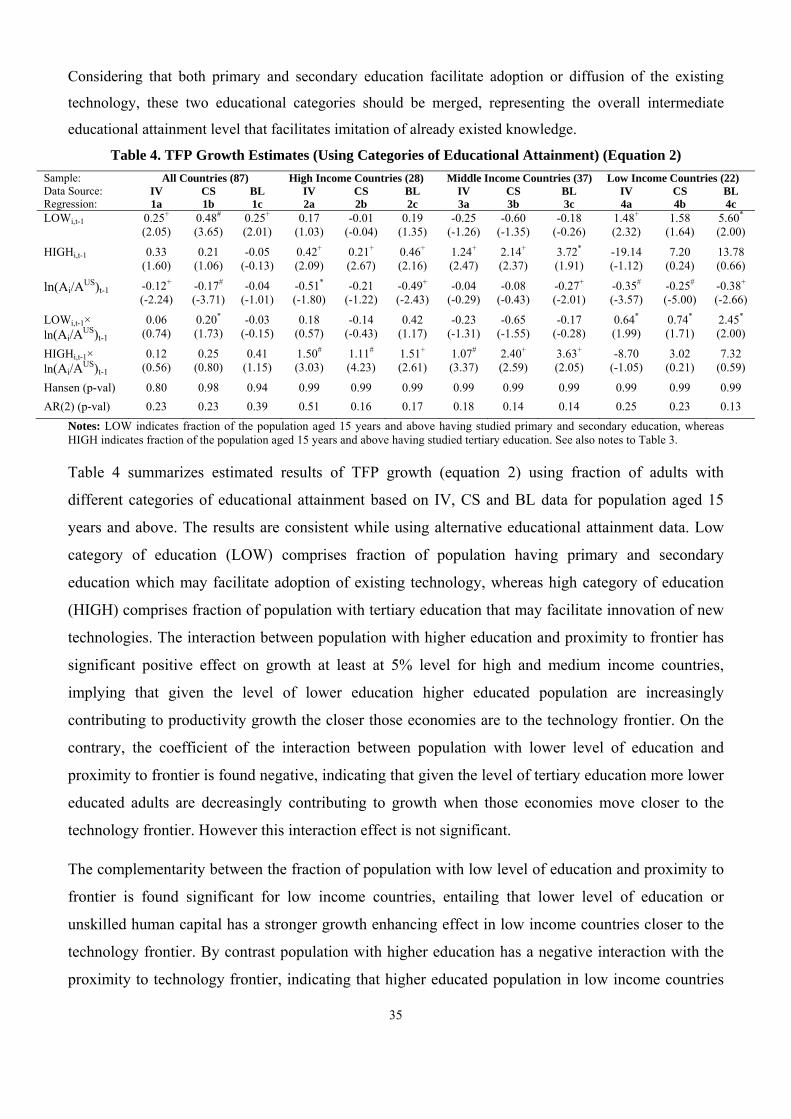
35

 

Considering that both primary and secondary education facilitate adoption or diffusion of the existing

technology, these two educational categories should be merged, representing the overall intermediate

educational attainment level that facilitates imitation of already existed knowledge.

Table 4. TFP Growth Estimates (Using Categories of Educational Attainment) (Equation 2)

Sample: All Countries (87) High Income Countries (28) Middle Income Countries (37) Low Income Countries (22) Data Source: IV CS BL IV CS BL IV CS BL IV CS BL Regression: 1a 1b 1c 2a 2b 2c 3a 3b 3c 4a 4b 4c LOWi,t-1 0.25+

(2.05) 0.48# (3.65)

0.25+ (2.01)

0.17 (1.03)

-0.01 (-0.04)

0.19 (1.35)

-0.25 (-1.26)

-0.60 (-1.35)

-0.18 (-0.26)

1.48+ (2.32)

1.58 (1.64)

5.60* (2.00)

HIGHi,t-1 0.33 (1.60)

0.21 (1.06)

-0.05 (-0.13)

0.42+ (2.09)

0.21+ (2.67)

0.46+ (2.16)

1.24+ (2.47)

2.14+ (2.37)

3.72* (1.91)

-19.14 (-1.12)

7.20 (0.24)

13.78 (0.66)

ln(Ai/AUS)t-1 -0.12+ (-2.24)

-0.17# (-3.71)

-0.04 (-1.01)

-0.51* (-1.80)

-0.21 (-1.22)

-0.49+ (-2.43)

-0.04 (-0.29)

-0.08 (-0.43)

-0.27+ (-2.01)

-0.35# (-3.57)

-0.25# (-5.00)

-0.38+ (-2.66)

LOWi,t-1× ln(Ai/AUS)t-1

0.06 (0.74)

0.20* (1.73)

-0.03 (-0.15)

0.18 (0.57)

-0.14 (-0.43)

0.42 (1.17)

-0.23 (-1.31)

-0.65 (-1.55)

-0.17 (-0.28)

0.64* (1.99)

0.74* (1.71)

2.45* (2.00)

HIGHi,t-1× ln(Ai/AUS)t-1

0.12 (0.56)

0.25 (0.80)

0.41 (1.15)

1.50# (3.03)

1.11# (4.23)

1.51+ (2.61)

1.07# (3.37)

2.40+ (2.59)

3.63+ (2.05)

-8.70 (-1.05)

3.02 (0.21)

7.32 (0.59)

Hansen (p-val) 0.80 0.98 0.94 0.99 0.99 0.99 0.99 0.99 0.99 0.99 0.99 0.99 AR(2) (p-val) 0.23 0.23 0.39 0.51 0.16 0.17 0.18 0.14 0.14 0.25 0.23 0.13

Notes: LOW indicates fraction of the population aged 15 years and above having studied primary and secondary education, whereas HIGH indicates fraction of the population aged 15 years and above having studied tertiary education. See also notes to Table 3.

Table 4 summarizes estimated results of TFP growth (equation 2) using fraction of adults with

different categories of educational attainment based on IV, CS and BL data for population aged 15

years and above. The results are consistent while using alternative educational attainment data. Low

category of education (LOW) comprises fraction of population having primary and secondary

education which may facilitate adoption of existing technology, whereas high category of education

(HIGH) comprises fraction of population with tertiary education that may facilitate innovation of new

technologies. The interaction between population with higher education and proximity to frontier has

significant positive effect on growth at least at 5% level for high and medium income countries,

implying that given the level of lower education higher educated population are increasingly

contributing to productivity growth the closer those economies are to the technology frontier. On the

contrary, the coefficient of the interaction between population with lower level of education and

proximity to frontier is found negative, indicating that given the level of tertiary education more lower

educated adults are decreasingly contributing to growth when those economies move closer to the

technology frontier. However this interaction effect is not significant.

The complementarity between the fraction of population with low level of education and proximity to

frontier is found significant for low income countries, entailing that lower level of education or

unskilled human capital has a stronger growth enhancing effect in low income countries closer to the

technology frontier. By contrast population with higher education has a negative interaction with the

proximity to technology frontier, indicating that higher educated population in low income countries

36

 

are decreasingly contributing to growth when they approach the frontier. However this interaction

effect is insignificant. The effect of lagged proximity to frontier on productivity growth is found

negative and significant for low income countries, implying the evidence of technology convergence

independent of human capital. The estimated results are consistent across total as well as working age

population for both the age groups (15 & 25 years and above) (see appendix Table A5).

Table 5. TFP Growth Estimates (Using Years of Educational Attainment) (Equation 3)

Sample: All Countries (87) High Income Countries (28) Middle Income Countries (37) Low Income Countries (22) Data Source: IV CS BL IV CS BL IV CS BL IV CS BL Regression: 1a 1b 1c 2a 2b 2c 3a 3b 3c 4a 4b 4c YPSi,t-1 0.02*

(1.95) 0.02+ (2.34)

0.01 (1.57)

-0.02 (-1.42)

-0.003 (-0.25)

0.01 (1.09)

-0.02 (-0.56)

-0.01 (-0.63)

0.01 (0.29)

0.16+ (2.22)

0.21# (5.22)

0.24+ (2.15)

YTERi,t-1 -0.02 (-0.19)

-0.07 (-1.20)

-0.08 (-1.39)

0.20# (3.62)

0.05 (1.35)

0.03 (1.21)

0.48+ (2.16)

0.54# (2.77)

0.34 (1.07)

-5.28 (-1.22)

-2.13 (-0.88)

-4.88 (-1.17)

ln(Ai/AUS)t-1 -0.08+ (-2.05)

-0.10+ (-2.58)

-0.02 (-0.33)

-0.06 (-0.22)

-0.26 (-1.12)

-0.59+ (-2.50)

-0.06 (-0.32)

-0.11 (-0.62)

-0.26+ (-2.13)

-0.30# (-3.37)

-0.42# (-7.53)

-0.32* (-1.98)

YPSi,t-1× ln(Ai/AUS)t-1

-0.0001 (-0.02)

0.003 (0.52)

-0.006 (-0.70)

-0.05* (-1.73)

-0.01 (-0.42)

0.02 (1.20)

-0.04 (-1.22)

-0.02 (-1.00)

-0.003 (-0.18)

0.07* (1.83)

0.10# (5.72)

0.10+ (2.10)

YTERi,t-1× ln(Ai/AUS)t-1

0.02 (0.21)

0.05 (0.61)

0.13 (1.64)

0.77# (4.31)

0.30+ (2.19)

0.13+ (2.10)

0.51# (3.11)

0.63# (3.24)

0.48* (1.88)

-2.34 (-1.10)

-1.14 (-0.89)

-2.21 (-0.95)

Hansen (p-val) 0.81 0.41 0.59 0.99 0.99 0.99 0.99 0.99 0.99 0.99 0.99 0.99 AR(2) (p-val) 0.38 0.17 0.36 0.79 0.31 0.12 0.13 0.11 0.13 0.23 0.12 0.20

Notes: YPS indicates years of primary and secondary education of the fraction of population aged 15 years and above, whereas YTER indicates years of tertiary education of the fraction of population aged 15 years and above. See also notes to Table 3.

Table 5 reports estimated results of TFP growth (equation 3) allowing the stocks of skilled (population

having tertiary education) and unskilled (population having primary and secondary education) human

capital to vary independently. It is assumed that a college graduate contributes twelve years to lower

level of education (primary & secondary) and four years to higher level of education (tertiary). Using

human capital composition data from IV, CS and BL, the estimated results are found consistent in

population aged 15 years and above. The estimated results are very similar as illustrated in Table 4.

The interaction between the years of tertiary education (YTER) and proximity to frontier has

significant positive effect on growth, whereas the interaction between the years of primary and

secondary education (YPS) and proximity to frontier has negative effect on growth though

insignificant for high as well as medium income countries, implying that given the level of primary

and secondary education tertiary education is more growth enhancing for high and medium income

countries closer to technology frontier, whereas given the level of tertiary education primary and

secondary education are decreasingly contributing to growth as high and medium income countries

approaches to technological frontier. In contrast, the years of primary and secondary education have

significant positive interaction with the proximity to frontier, whereas the years of tertiary education

have negative but insignificant interaction with the proximity to frontier for low income countries,

implying that growth enhancing effect of primary and secondary (tertiary) education increases

(decreases) as low income countries move closer to technology frontier. The effect of lagged

37

 

proximity to frontier on growth is found negative and significant for low income countries showing

the potential for technology convergence independent of human capital. The only noticeable

difference is that coefficients on educational attainment levels, such as primary, secondary and tertiary

and their interaction with proximity to technology frontier are now much smaller. The estimated

results are consistent across total as well as working age population for both the age groups (15 & 25

years and above) (see appendix Table A6).

Table 6. TFP Growth Estimates (Using Years of Skilled and Unskilled Education) (Equation 4)

Sample: All Countries (87) High Income Countries (28) Middle Income Countries (37) Low Income Countries (22) Data Source: IV CS BL IV CS BL IV CS BL IV CS BL Regression: 1a 1b 1c 2a 2b 2c 3a 3b 3c 4a 4b 4c YUSKi,t-1 0.02*

(1.95) 0.02# (2.73)

0.01 (1.36)

0.001 (0.14)

-0.002 (-0.25)

0.01 (0.70)

-0.02 (-0.56)

-0.02 (-0.66)

0.01 (0.21)

0.09+ (2.22)

0.21# (5.28)

0.21* (1.86)

YSKi,t-1 0.01 (0.65)

-0.002 (-0.35)

0.002 (0.38)

0.02*

(1.86) 0.01+ (2.66)

0.01+ (2.37)

0.11+ (2.36)

0.10# (3.20)

0.06 (1.40)

-0.001 (-0.01)

-0.22 (-0.51)

-0.54 (-0.74)

ln(Ai/AUS)t-1 -0.08+ (-2.05)

-0.07* (-1.79)

-0.02 (-0.37)

-0.34 (-1.63)

-0.27 (-1.15)

-0.52+ (-2.04)

-0.06 (-0.32)

-0.10 (-0.56)

-0.24* (-1.82)

-0.25+ (-4.21)

-0.42# (-7.41)

-0.30* (-1.83)

YUSKi,t-1× ln(Ai/AUS)t-1

-0.0001 (-0.02)

-0.002 (-0.31)

-0.01 (-0.78)

-0.003 (-0.11)

-0.01 (-0.39)

0.02 (0.88)

-0.04 (-1.22)

-0.02 (-1.05)

-0.01 (-0.27)

0.03* (1.73)

0.09# (5.77)

0.10* (1.82)

YSKi,t-1× ln(Ai/AUS)t-1

0.004 (0.26)

0.01 (1.27)

0.01 (1.62)

0.09# (3.15)

0.05# (3.23)

0.03# (3.22)

0.10# (3.61)

0.11# (3.57)

0.08+ (2.02)

0.02 (0.08)

-0.13 (-0.54)

-0.24 (-0.57)

Hansen (p-val) 0.77 0.99 0.99 0.99 0.99 0.99 0.99 0.99 0.99 0.99 0.99 0.99 AR(2) (p-val) 0.38 0.31 0.34 0.57 0.31 0.11 0.13 0.11 0.13 0.22 0.13 0.16

Notes: YUSK indicates years of unskilled educational attainment of the fraction of population aged 15 years and above, whereas YSK indicates years of skilled educational attainment of the fraction of population aged 15 years and above. See also notes to Table 3.

Table 6 presents estimated results of TFP growth (equation 4) allowing alternative definition of

skilled and unskilled labor force. It is assumed that a college graduate contributes 16 years to years of

skilled education (YSK) and zero (0) years to years of unskilled education (YUSK). Estimated results

using human capital composition data from IV, CS and BL are found consistent in population aged 15

years and above. The results are broadly similar to those obtained in the earlier specifications as

illustrated in Table 4. The only noticeable difference is that coefficients on skilled as well as unskilled

human capital are now significantly smaller similar to the results found in Table 5. The estimated

results are consistent across total as well as working age population for both the age groups (15 & 25

years and above) (see appendix Table A7).

Demographic dimension of the different levels of human capital may have important impact on

productivity growth. Barro and Lee (1994) obtain a significantly negative coefficient on female

education and a significantly positive one on male education. Caselli et al. (1996) find the exact

opposite. Both results are puzzling because, whereas different models lead to different predictions on

the expected sign of the coefficient on the human capital variables, there is no theory that is consistent

with different signs for male and female human capital. However, it often has been documented that

there is a strong negative relationship between female education and fertility rates, and an equally

38

 

strong negative relationship between fertility rates and growth rates (Barro and Sala-i-Martin, 1995; Barro

and Lee, 1994). Therefore, female education captures both (positive) fertility effects, and (negative)

human capital effects, and hence the former outweighs the latter. Male education only represents a human

capital effect and thus it produces negative coefficient (Caselli et al., 1996). Table 7. TFP Growth Estimates (Using SEX-wise Fraction of Educational Attainment) (Equation 1)

All Countries (87) High Income Countries (28)

Middle Income Countries (37)

Low Income Countries (22)

Male Female Male Female Male Female Male Female PRIi,t-1 0.17

(1.36) 0.16 (1.40)

0.25 (1.34)

0.07 (0.47)

-0.17 (-0.89)

-0.28 (-1.49)

-0.02 (-0.05)

-1.32 (-1.26)

SECi,t-1 0.34# (2.97)

0.09 (0.78)

0.22 (1.23)

0.07 (0.49)

0.04 (0.17)

-0.01 (-0.02)

2.56+ (2.65)

8.64# (3.90)

TERi,t-1 -0.03 (-0.13)

0.49* (1.73)

0.55+ (2.16)

0.41+ (2.04)

1.30+ (2.37)

1.36# (2.91)

-8.97 (-1.45)

-36.61 (-1.19)

ln(Ai/AUS)t-1 -0.09* (-1.93)

-0.09+ (-2.00)

-0.63* (-1.81)

-0.33 (-1.43)

-0.15 (-1.33)

-0.08 (-0.85)

-0.25# (-3.58)

-0.28 (-1.58)

PRIi,t-1× ln(Ai/AUS)t-1 0.01 (0.16)

0.08 (0.97)

0.30 (0.73)

-0.04 (-0.13)

-0.07 (-0.40)

-0.20 (-1.14)

-0.07 (-0.30)

-0.68 (-1.42)

SECi,t-1× ln(Ai/AUS)t-1 0.10 (1.04)

-0.15 (-1.14)

0.22 (0.65)

0.03 (0.11)

-0.09 (-0.50)

-0.13 (-0.63)

1.22+ (2.49)

4.49# (4.10)

TERi,t-1× ln(Ai/AUS)t-1 -0.20 (-0.63)

0.61* (1.85)

1.82# (2.80)

1.31+ (2.51)

1.22# (3.31)

1.21# (3.75)

-4.65 (-1.39)

-18.75 (-1.38)

Hansen (p-value) 0.97 0.51 0.99 0.99 0.99 0.99 0.99 0.99 AR(2) (p-value) 0.54 0.19 0.51 0.55 0.12 0.16 0.12 0.17

Notes: see notes to Table 3.  

Table 7 summarizes estimated results of TFP growth (equation 1) using IV’s sex-wise fraction of different

levels of educational attainment for population aged 15 years and above. Estimated coefficients of the

interaction between the fraction of population with tertiary education and proximity to technology frontier

are found positive and significant for both male and female in high and medium income countries, whereas

the fraction of population with secondary education has significant positive interaction with the proximity

to frontier for both male and female in low income countries. The coefficients of proportions of female

population with tertiary education are found marginally lower than the male in high and medium countries,

whereas female workers with secondary education are observed significantly higher than male in low

income countries. Therefore, both male and female labor with different educational attainment level have

significant contribution to productivity growth irrespective of country groups though the contribution of

unskilled female population is significantly higher in low income countries. The estimated results are

consistent across total as well as working age population aged 25 years and above (not reported).

Finally, this study attempts to examine the effect of age-wise fraction of population attained different

levels of education on productivity growth. Educational attainment data provided by IIASA & VID

(IV)(2007) only allows age and sex wise distribution of different levels of human capital and hence this

study solely depends on this database to examine the demographic dimensions of the composition of

human capital (skilled and unskilled). Table 8 presents estimated results of TFP growth (equation 1)

across different groups of workers aged 20 years and above into 15-year intervals (20-34, 35-49, 50-64).

39

 

Table 8. TFP Growth Estimates (Using AGE-wise Fraction of Educational Attainment) (Equation 1) All Countries (87) High Income Countries (28) Middle Income Countries (37) Low Income Countries (22)

Age Groups 20-34 35-49 50-64 20-34 35-49 50-64 20-34 35-49 50-64 20-34 35-49 50-64 PRIi,t-1 0.07

(0.30) 0.09 (0.76)

0.08 (1.15)

0.10 (0.33)

0.14 (0.76)

0.06 (0.63)

-0.32 (-1.22)

-0.26 (-1.31)

-0.01 (-0.03)

0.24 (0.50)

-0.08 (-0.21)

-0.08 (-0.13)

SECi,t-1 0.35+ (2.06)

0.15 (1.39)

0.09 (1.10)

0.21 (0.99)

0.10 (0.56)

0.004 (0.04)

0.05 (0.26)

-0.10 (-0.46)

-0.22 (-0.54)

1.35+ (2.03)

3.58+ (2.10)

3.51 (1.06)

TERi,t-1 0.07 (0.32)

0.21 (1.49)

0.28 (1.33)

0.40 (1.47)

0.40+

(2.13) 0.49+

(2.64) 0.78 (1.57)

0.96+ (2.66)

2.04+ (2.12)

-1.89 (-0.26)

-9.33 (-1.26)

-2.13 (-0.15)

ln(Ai/AUS)t-1 -0.13 (-1.51)

-0.07 (-1.54)

-0.06* (-1.76)

-0.61 (-1.56)

-0.46 (-1.36)

-0.31+ (-2.15)

-0.11 (-0.80)

-0.09 (-0.72)

-0.20 (-1.44)

-0.28# (-3.72)

-0.21# (-4.71)

-0.16# (-3.41)

PRIi,t-1× ln(Ai/AUS)t-1

-0.01 (-0.07)

0.01 (0.20)

-0.0001 (-0.02)

0.08 (0.15)

0.14 (0.39)

0.06 (0.27)

-0.18 (-0.86)

-0.15 (-0.82)

-0.05 (-0.19)

0.06 (0.27)

-0.11 (-0.59)

-0.11 (-0.36)

SECi,t-1× ln(Ai/AUS)t-1

0.17 (1.57)

-0.01 (-0.09)

-0.15 (-1.62)

0.30 (0.80)

0.06 (0.16)

-0.09 (-0.37)

-0.01 (-0.09)

-0.18 (-0.98)

-0.43 (-1.59)

0.64*

(1.87) 1.75* (1.97)

1.67 (0.96)

TERi,t-1× ln(Ai/AUS)t-1

-0.40 (-1.38)

0.10 (0.56)

0.42+ (2.36)

1.21+

(2.04) 1.31#

(2.85) 1.57+

(2.37) 0.75* (1.68)

0.90# (3.85)

1.74# (3.15)

-1.18 (-0.30)

-4.68 (-1.24)

-0.62 (-0.10)

Hansen (p-val) 0.99 0.99 0.99 0.99 0.99 0.99 0.99 0.99 0.99 0.99 0.99 0.99 AR(2) (p-val) 0.56 0.66 0.23 0.59 0.52 0.41 0.12 0.13 0.11 0.19 0.12 0.18

Notes: see notes to Table 3.

The interaction between the fraction of population with tertiary education and proximity to frontier is

found strong positive and significant for the matured age group (35-49, 50-64 years) in high and medium

income countries, whereas a positive and significant interaction effect between the fraction of population

with secondary education and proximity to technology frontier has been found for the younger population

(20-34 years) in low income countries. Therefore, increase in younger population with secondary

education could be the key driver for productivity growth for low income countries as they move closer to

technology frontier, whereas tertiary education with more matured workers contributes more to

productivity growth for high and middle income countries as they approach technology frontier. This

empirical result is consistent with the findings of Crespo and Lutz (2007).

6.2.1. Robustness Checks

The relationship between human capital and growth is likely to be affected by severe problems of

endogeneity (Bils and Klenow, 2000). Although system GMM estimator may capture unobserved

heterogeneity and possible endogeneity in the model, still there could be endogeneity as well as omitted

variable bias and thus a robustness check is desirable. Hence this study considers lagged public

expenditure on education in different educational level as external instrument for different level of human

capital. Although system GMM estimator is primarily designed for internal instruments (lagged

differences and lagged levels of the explanatory variables) but it does allow external instruments to deal

with endogeneity problem (Roodman, 2009). Data on public educational expenditure in several developing

countries, such as Brazil, Argentina, Gabon, Nigeria and so on are found to have sudden fluctuations most

probably due to the change in currency denomination and therefore use of public expenditure needs to

compromise with number of observation especially for low and medium income countries.

40

 

Appendix Table A8 reports estimated results by re-estimating TFP growth (equation 1) after allowing

public educational expenditure on different levels as instruments for different level of educational

attainment. The results are by and large very similar to those of the baseline results reported in Table 3.

Growth enhancing effect of tertiary education increases as high and medium income countries move closer

to the technology frontier, whereas growth enhancing effect of secondary education increases as low

income countries approaches technology frontier. This study also re-estimates TFP growth (equation 1) in

10-year differences and found similar results (not reported). Hence empirical results are less likely to be

affected by endogeneity. For further robustness check, this study also re-estimates TFP growth (equation

1) by incorporating three additional control variables, such as financial development proxied by the ratio

of private credit to GDP (PC), geographical location measured by landlockness (LOCK) and institutional

development proxied by political risk (PR). The estimated results reported in Appendix Table A9 remain

very similar to those of the baseline results (Table 3). Therefore the empirical findings of this study are

less likely to be affected by omitted variable bias.

VII. Concluding Remarks

Human capital is generally considered as an important factor to accelerate economic growth though

empirical evidences till today are mixed. Some argue that human capital should enter into production

function as an input and thereby affects output growth directly, while others argue that human capital

contribute to raise technological progress by easing innovation, diffusion and adoption of new

technologies and thus affects productivity growth indirectly. It is also reasonable that different kinds and

levels of human capital may have different effects on growth. The effect of human capital composition on

growth has been gained momentum in the most recent endogenous growth models. Assuming that the

technological progress is a dual mechanism comprises of innovation and imitation and that primary and

secondary education are more suitable for imitation and higher education is more appropriate for

innovation, this study aims to investigate whether the contribution of human capital to productivity growth

depends on the composition of human capital and the proximity to technology frontier in a panel of 87

sample countries consisting of 28 high, 37 medium and 22 low income countries over the period of 1970

to 2004. Furthermore, it investigates the evidence of technology convergence independent of human

capital. It uses different levels of educational attainment data for available age groups from four standard

sources of human capital data such as, BL (2001), DD (2006), CS (2007) and IV (2007) though it has

emphasized more on IV data which are available across sex and age distribution (5-year interval). It

applies three different estimators, such as pooled OLS, fixed effects and system GMM though the system

GMM estimator has been preferred to deal with endogeneity problem. The estimated results are found to

be consistent and robust in alternative sources of human capital and hence they are not likely to be induced

by unobserved country specific effects, endogeneity, simultaneity, and omitted variables biases.

41

 

The empirical results in this study demonstrate that growth enhancing effects of skilled human capital

(measured by the fraction of population with tertiary education) increases as high and medium income

countries move closer to the technology frontier. In other words, those economies concentrate more on

innovation than imitation and thus investment in tertiary education could accelerate TFP growth as their

technological gap narrows. Growth effect of primary and secondary education for those economy

decreases as they move closer to the technology frontier. On the other hand, growth enhancing effects of

unskilled human capital (measured by the combination of the proportion of population with primary and

secondary education) improves as low income countries approach technology frontier. In reality, those low

income countries are far away from the world technology frontier and they use to imitate technologies

already developed elsewhere and therefore, investment in secondary education could enhance their

productivity growth as they move closer to the technology frontier. Furthermore, there are evidences for

technology convergence independent of human capital in low income countries, implying that countries

those are far behind the technology frontier experience faster TFP growth.

Turing to the demographic dimensions of different levels of human capital, this study identifies significant

effect of the proportion of both male and female adults with different level of educational attainment in

explaining differences in the productivity growth across countries over time. As countries approach

technology frontier, both male and female workers with tertiary education contribute more to productivity

growth for high and medium income countries though the magnitude of the contribution of male is

relatively higher than that of the female, whereas both male and female labor with secondary education

contribute more to productivity growth for low income countries though the magnitude of the contribution

of female labor is significantly higher than that of the male. Increase in younger population with secondary

education is found the key driver for growth in low income countries, whereas tertiary education with

more matured population contributes more to productivity growth in high and medium income countries as

they move closer to the technology frontier.

The findings of this study have some important policy implications for high, medium and low income

countries. First, high and medium income countries-those invest more in tertiary education will continue to

grow as they move closer to the technology frontier. Second, low income countries-those invest more in

secondary education will continue to grow as they approach technology frontier. Third, tertiary

(secondary) education of both male and female adults are important for high and medium (low) income

countries though female education should be encouraged more in low income countries to experience

higher economic growth closer to the technology frontier. Finally, supply of unskilled younger workers in

low income countries and skilled matured workers in high income countries should be increased more to

experience higher economic growth as they move closer to the technology frontier. Quantity as well as

quality of human capital is important for growth (Lee and Barro, 2001) and thus examining the effects of

quality of human capital on productivity growth could be a scope for further research.

42

 

References

Abromovitz, M. (1986). "Catching up, Forging ahead, and Falling behind." Journal of Economic History 46: 386-406.

Acemoglu, D. (1996). "A Microfoundation for Social Increasing Returns in Human Capital Accumulation." Quarterly Journal of Economics 111: 779-804.

Acemoglu, D. (2002). "Technical Change, Inequality and The Labor Market." Journal of Economic Literature 40: 7-72.

Acemoglu, D., P. Aghion and F. Zilibotti (2002). "Distance to Frontier, Selection, and Economic Growth." Journal of the European Economic Association 4(1): 37-74.

Aghion, P., L. Boustan, C. Hoxby and J. Vandenbussche (2005). "Exploiting State's Mistakes to Identify the Causal Impact of Higher Education on Growth." NBER Conference Paper.

Aghion, P., L. Boustan, C. Hoxby and J. Vandenbussche (2009). "The Causal Impact of Education on Economic Growth: Evidence from U.S." Working Paper, Harvard University.

Aghion, P. and P. Howitt (1992). "A Model of Growth through Creative Destruction." Econometrica 60: 323-351.

Aghion, P. and P. Howitt (1998). Endogenous Growth Theory. Cambridge, MA, MIT Press. Anderson, T. and C. Hsiao (1982). "Formulation and Estimation of Panel Data." Journal of Econometrics

18: 47-82. Arellano, M. and S. R. Bond (1991). "Some tests for specification in panel data: Monte Caro evidence and

an application to employment equations." Review of Economic Studies 58: 277-297. Arellano, M. and O. Bover (1995). "Another look at the instrumental variables estimation or error

components models." Journal of Econometrics 68(1): 29-52. Azariadis, C. and A. Drazen (1990). "Threshold externalities in economic development." Quarterly Journal

of Economics 105(2): 501–526. Barro, R. J. (1991). "Economic growth in a cross section of countries." Quarterly Journal of Economics

106(2): 407–443. Barro, R. J. (1997). Determinants of Economic Growth: A Cross-Country Empirical Study. Cambridge,

M.A., MIT Press. Barro, R. J. (1999). "Human capital and growth in cross-country regressions." Swedish Economic Policy

Review 6(2): 237–277. Barro, R. J. (2001). "Education and Economic Growth." Mimeo, Harvard University. Barro, R. J. and J. W. Lee (1993). " International comparisons of educational attainment." Journal of

Monetary Economics 32(3): 363–394. Barro, R. J. and J. W. Lee (1994). "Sources of Economic Growth." Carnegie-Rochester Conference Series

on Public Policy 40: 1-46. Barro, R. J. and J. W. Lee (1996). " International measures of schooling years and schooling quality."

American Economic Review 86(2): 218–223. Barro, R. J. and J. W. Lee (2001). "International Data on Educational Attainment: Updates and

Implications." Oxford Economic Papers 53(3): 541-563. Barro, R. J. and X. Sala-i-Martin (1995). Economic Growth. New York, Mac Graw-Hill. Baum, C. F. (2006). An Introduction to Modern Econometrics Using Stata, College Station, TX, Stata

Press. Baum, C. F., M. E. Schaffer and S. Stillman (2003). "Instrumental variables and GMM: Estimation and

Testing." Stata Journal 3(1): 1-31. Beck, T., R. Levine and N. Loayza (2000). "Finance and the Sources of Growth." Journal of Financial

Economics 58: 261-310. Becker, G. S. (1975). Human capital: a theoretical and empirical analysis, Columbia University Press and

National Bureau of Economic Research, New York. Benhabib, J. and M. M. Spiegel (1994). "The role of human capital in economic development Evidence

from aggregate cross-country data." Journal of Monetary Economics 34: 143-173. Benhabib, J. and M. M. Spiegel (2005). Human Capital and Technology Diffusion. Handbook of

Economic Growth. P. Aghion and S. N. Durlauf. 1A: 935-966.

43

 

Bils, M. and P. J. Klenow (2000). "Does Schooling Cause Growth?" The American Economic Review 90(5): 1160-1183.

Blundell, R. and S. R. Bond (1998). "Initial conditions and moments restrictions in dymanic panel data models." Journal of Econometrics 87: 115-143.

Bosworth, B. P. and S. M. Collins (2003). "The Empirics of Growth: An Update." Brookings Papers on Economic Activity 2: 113-206.

Card, D. and A. Krueger (1992). "Does school quality matter? Returns to education and the characteristics of public schools in the United States." Journal of Political Economy 100: 1-40.

Caselli, F. (2005). Accounting for Cross-Country Income Differences. Handbook of Economic Growth. P. Aghion and S. N. Durlauf, Elsevier B.V. 1A.

Caselli, F., G. Esquivel and F. Lefort (1996). "Reopening the convergence debate: a new look at cross-country empirics. Journal of Economic Growth " 1: 363–389.

Castello, A. (2006). "On the distribution of Education and Democracy." Institute of International Economics Working paper No. 0602, University of Valencia.

Chowdhury, K. P. (1995). "Literacy and primary education." Human Capital Development and Operations Policy Working Papers 50, World Bank, Washington D.C.

Cohen, D. and M. Soto (2007). "Growth and human capital: good data, good results." Journal of Economic Growth 12: 51-76.

Collins, S. M. and B. P. Bosworth (1996). "Economic growth in east Asia: accumulation versus assimilation." Brookings Papers on Economic Activity 2: 135–203.

Crespo, C. J. and W. Lutz (2007). "Human Capital, Age Structure and Economic Growth: Evidence from a New Dataset." IIASA Interim Report IR-07-011, Laxenburg,Austria: International Institute for Applied Systems Analysis.

De la Fuente, A. and R. Dom´enech (2006). "Human capital in growth regressions: How much difference does data quality make?" Journal of the European Economic Association 4(1): 1-36.

De la Fuente, A. and R. Domenech (2001). "Schooling data, technological diffusion, and the neoclassical model." The American Economic Review, Papers and Proceedings 91: 323-327.

Durlauf, S. N. and P. A. Johnson (1995). "Multiple Regimes and Cross-Country Growth Behaviour." Journal of Applied Econometrics 10(4): 365-384.

Easterlin, R. E. (1981). "Why Isn't The Whole World Developed?" Journal of Economic History 41(1): 1-19.

Engelbrecht, H-J. (2003). "Human Capital and Economic Growth: Cross-Section Evidence for OECD Countries." The Economic Record 79: S40–S51.

Fama, E. F. and K. R. French (2006). "Profitability, investment and average returns." Journal of Financial Economics 82: 491–518.

Gemmell, N. (1996). "Evaluating the impacts of human capital stocks and accumulation on economic growth: Some new evidence." Oxford Bulletin of Economics and Statistics 58(1): 9–28.

Gerschenkron, A. (1962). Economic backwardness in historical perspective. Cambridge, Belknap Press of Harvard University Press.

Gollin, D. (2002). "Getting Income Shares Right." Journal of Political Economy 110(2): 458-474. Greene, H. W. (2003). Econometric Analysis, 5th Edition, Prentice Hall. Grossman, G. M. and E. Helpman (1991). Innovation and Growth in the Global Economy. Cambridge,

MA, MIT Press. Ha, J., J. Y. Kim and J.-W. Lee (2009). "The Optimal Structure of Technology Adoption and Creation:

Basic Research vs. Development in the Presence of Distance to Frontier." ADB Economics Working Paper No. 163, Asian Development Bank.

Hanushek, E. (1986). "The economics of schooling: production and efficiency in public schools." Journal of Economic Literature 24: 1141-1177.

Hanushek, E. (1995). "Interpreting Recent Research on Schooling in Developing Countries." World Bank Research Observer 10: 227-246.

Hanushek, E. and D. Kimko (2000). "Schooling, Labour Force Quality and the Growth of Nations." American Economic Review 90: 1184-1208.

Hanushek, E. and L. Wossmann (2007). Education Quality and Economic Growth. Washington DC, The

44

 

World Bank. Hanushek, E. and L. Woessmann (2008). "The Role of Cognitive Skills in Economic Development."

Journal of Economic Literature 46: 607-668. Hayashi, F. (2000). Econometrics, Princeton University Press. Heston, A., R. Summers and B. Aten (2006). Penn World Table Version 6.2, Center for International

Comparisons of Production, Income and Prices, University of Pennsylvania. Hoeffler, A. E. (2000). "The Augmented Solow Model and the African Growth Debate." CID Working

Paper No. 36, Center for International Development, Harvard University. Hojo, M. (2003). "An indirect effect of education on growth." Economics Letters 80: 31–34. IIASA (2008). Economic Growth in Developing Countries: Education Proves Key. International Institute

for Applied Systems Analysis (IIASA) Policy Brief #03, Austrian Academy of Sciences, Austria. Islam, N. (1995). "Growth empirics: A panel data approach." Quarterly Journal of Economics 110(4):

1127–1170. Jones, G. (2008). "Cognitive ability and technology diffusion: An empirical test." American Economic

Association Annual Meeting. Jones, G. and W. J. Schneider (2006). "Intelligence, human capital, and economic growth: A Bayesian

averaging of classical Estimates (BACE) Approach,." Journal of Economic Growth 11(1): 71-93. Judson, R. (2002). "Measuring human capital like physical capital: What does it tell us?" Bulletin of

Economic Research 54(3): 209–231. Kalaitzidakis, P., T. P. Mamuneas, A. Savvides and T. Stengos ( 2001). "Measures of Human Capital and

Non-Linearities in Economic Growth." Journal of Economic Growth 6: 229-254. Kneller, R. and P. A. Stevens (2006). "Frontier Technology and Absorptive Capacity: Evidence from

OECD Manufacturing Industries." Oxford Bulletin of Economics and Statistics 68(1): 1-21. Knowles, S. and P. D. Owen (1995). "Health capital and cross-country variation in income per capita in

Mankiw–Romer–Weil model." Economics Letters 48: 99–106. Krueger, A. (1999). "Experimental estimates of education production functions." Quarterly Journal of

Economics 114: 497-532. Krueger, A. B. and M. Lindahl (1999). "Education for growth in Sweden and the world." Swedish

Economic Policy Review 6(2): 289-339. Krueger, A. B. and M. Lindahl (2001). "Education for Growth: Why and For Whom?" Journal of

Economic Literature 39(4): 1101-1136. Kyriacou, G. (1991). " Level and growth effects of human capital: A cross-country study of the

convergence hypothesis." Economic Research Reports 91-26, New York University. Lau, L. J., D. T. Jamison and F. F. Louat (1991). "Education and productivity in developing countries: An

aggregate production function approach." Policy, Research, and External AffairsWorking Paper 612, World Bank, Washington D.C.

Le, T., J. Gibson and L. Oxley (2005). "Measures of Human Capital: A Review of the Literature." New Zealand Treasury Working Paper 05/10, Wellington, New Zealand.

Lee, J. W. and R. J. Barro (2001). "Schooling Quality in a Cross-Section of Countries." Economica 68: 465-488.

Levine, R. and D. Renelt (1992). "A Sensitivity Analysis of Cross-Country Growth Regressions." The American Economic Review, 82(4): 942-963.

Ljungberg, J. and A. Nilsson (2009). "Human capital and economic growth: Sweden 1870–2000." Cliometrica 3: 71-95.

Lucas, R. (1988). "On the mechanics of economic development " Journal of Monetary Economics 22: 3-42.

Lucas, R. E. J. (1990). "Why Doesn't Capital Flow from Rich to Poor Countries?" The American Economic Review 80(2): 92-96.

Lutz, W., J. C. Cuaresma and W. Sanderson (2008). "The Demography of Educational Attainment and Economic Growth." SCIENCE 319: 1047-1048.

Lutz, W., A. Goujon, K. C. Samir and W. Sanderson (2007). "Reconstruction of populations by age, sex and level of educational attainment for 120 countries for 1970-2000." Vienna Yearbook of Population Research 2007: 193-235.

45

 

Mankiw, G., D. Romer and D. N. Weil (1992). "A Contribution to the Empirics of Economic Growth." Quarterly Journal of Economics 107(2): 407-437.

Maria, C. D. and P. Stryszowski (2009). "Migration, human capital accumulation and economic development." Journal of Development Economics 90 306-313.

Mincer, J. (1974). Schooling, Experience, and Earnings. New York, Columbia University Press. Nehru, V., E. Swanson and A. Dubey (1995). "A new database in human capital stock in developing

industrial countries: Sources, methodology and results." Journal of Development Economics 46(2): 379–401.

Nelson, R. R. and E. S. Phelps (1966). "Investment in Humans, Technological Diffusion, and Economic Growth." The American Economic Review 56(1/2): 69-75.

Nickell, S. (1981). "Biases in dynamic models with fixed effects." Econometrica 49(6): 1417-1426. Nonneman, W. and P. Vanhoudt (1996). "A further augmentation of the Solow model and the empirics of

economic growth for OECD countries." Quarterly Journal of Economics 111: 943–953. OECD (1998). Human Capital Investment: An International Comparison, OECD Center for Educational

Research and Innovation, Paris. Papageorgioua, C. and F. Perez-Sebastianb (2006). "Dynamics in a non-scale R&D growth model with

human capital: Explaining the Japanese and South Korean development experiences." Journal of Economic Dynamics & Control 30: 901–930.

Portela, M., R. Alessie and C. Teulings (2004). "Measurement Error in Education and Growth Regressions." Tinbergen Institute Discussion Paper TI 2004-040/3, Universiteit Amsterdam.

Pritchett, L. (2001). "Where Has All the Education Gone?" The World Bank Economic Review 15(3): 367-391.

Psacharopoulos, G. and A. M. Arriagada (1986). "The educational composition of the labour force: An international comparison." International Labour Review 125(5): 561–574.

Psacharopoulos, G. and A. M. Arriagada (1992). "The educational composition of the labour force: An international update." Journal of Educational Planning and Administration 6(2): 141-159.

Radelet, S., J. Sachs, et al. (2001). "The Determinants And Prospects Of Economic Growth In Asia." International Economic Journal. 15(3): 1-29.

Romer, P. M. (1990a). "Endogenous Technological Change." Journal of Political Economy 98(5): S71-S102.

Romer, P. M. (1990b). "Human capital and growth: Theory and evidence." Carnegie-Rochester Conference Series on Public Policy 32: 251-286.

Roodman, D. (2009). " How to Do xtabond2: An Introduction to Difference and System GMM in Stata." The Stata Journal 9: 86-136.

Sala-i-Martin, X. X. (1997). "I Just Ran Two Million Regressions." The American Economic Review, 87(2): 178-183.

Schultz, T. W. (1960). "Capital formation by education." Journal of Political Economy 68(6): 571–583. Schultz, T. W. (1961). "Investment in human capital." American Economic Review 51(1): 1–17. Schultz, T. W. (1971). Investment in Human Capital: The Role of Education and of Research, The Free

Press, New York. Serrano, L. (2003). "Measurement error in schooling data: the OECD case." Applied Economics Letters

10(2): 73-75. Temple, J. (1998). "Robustness tests of the augmented Solow model." Journal of Applied Econometrics

13: 361–375. Temple, J. (1999). "A positive effect of human capital on growth." Economics Letters 65: 131–134. Topel, R. (1999). Labor markets and economic growth. Handbook of Labor Economics. O. Ashenfelter

and D. Card. Amsterdam, Elsevier: 2943-3029. UNESCO (1993). World Education Report, UNESCO, Paris. Vandenbussche, J., P. Aghion and C. Meghir (2006). "Growth, distance to frontier and composition of

human capital." Journal of Economic Growth 11: 97-127. Wolff, E. N. (2000). "Human capital investment and economic growth: Exploring the cross-country

evidence." Structural Change and Economic Dynamics, 11(4): 433-472.

46

 

Appendix

Table A1. Variable Sources and Definitions

Variable Source and Definition

∆lnA

Total Factor Productivity (TFP) Growth is calculated from the 6.2 version of the Penn World Table (PWT6.2-

Heston, Summers and Aten ,2006) available at, http://pwt.econ.upenn.edu/php_site/pwt_index.php

PRI

Fraction of the population having primary education , taken from Barro and Lee (2001) henceforth ‘BL’

available at http://www.cid.harvard.edu/ciddata/ciddata.html ; De la Fuente and Domenech (2006) henceforth

‘DD’ available at http://iei.uv.es/rdomenec/human/human.html ; Cohen and Soto (2007) henceforth ‘CS’

available at http://soto.iae-csic.org/Data.htm and International Institute for Applied Systems Analysis and

Vienna Institute of Demography (2007) henceforth ‘IV’ available at

http://www.iiasa.ac.at/Research/POP/edu07/index.html?sb=11.

SEC

Fraction of the population having secondary education , taken from Barro and Lee (2001) henceforth ‘BL’

available at http://www.cid.harvard.edu/ciddata/ciddata.html ; De la Fuente and Domenech (2006) henceforth

‘DD’ available at http://iei.uv.es/rdomenec/human/human.html ; Cohen and Soto (2007) henceforth ‘CS’

available at http://soto.iae-csic.org/Data.htm and International Institute for Applied Systems Analysis and

Vienna Institute of Demography (2007) henceforth ‘IV’ available at

http://www.iiasa.ac.at/Research/POP/edu07/index.html?sb=11.

TER

Fraction of the population having tertiary education , taken from Barro and Lee (2001) henceforth ‘BL’

available at http://www.cid.harvard.edu/ciddata/ciddata.html ; De la Fuente and Domenech (2006) henceforth

‘DD’ available at http://iei.uv.es/rdomenec/human/human.html ; Cohen and Soto (2007) henceforth ‘CS’

available at http://soto.iae-csic.org/Data.htm and International Institute for Applied Systems Analysis and

Vienna Institute of Demography (2007) henceforth ‘IV’ available at

http://www.iiasa.ac.at/Research/POP/edu07/index.html?sb=11.

ln(Ai /AUS)

Proximity (inverse of distance) to technology frontier is measured by the logarithm of relative productivity

(TFP) gap between the sample countries and the US, calculated from productivity growth (∆lnA) derivation as

stated above. Being the technology leader as well as the major trading partner of most of the countries, the US

technology is assumed here as the world technological frontier (AUS).

INF

Inflation Rate is measured by the consumer price index, taken from World Development Indicators (WDI)

2009 online database.

OP

Trade Openness is measured by the ratio of the sum of total exports and imports to GDP, taken from the

World Development Indicators (WDI) 2009 online database.

FDI

Inflow of Foreign Direct Investment (FDI) is measured by the ratio of foreign direct investment (FDI) inflow

to GDP, taken from World Development Indicators (WDI) 2009 online database.

PC

Private Sector Credit is measured by the ratio of financial resources provided to the private sector to GDP,

taken from World Development Indicators (WDI) 2009 online database.

PR

Institutional development is measured by the index of ‘Political Risk’, taken from Freedom House database

available at http://www.freedomhouse.org/template.cfm?page=1

LOCK

Geographical location is measured by ‘landlockness’, taken from Doing Business in Landlocked Economies

2009 database available at http://www.doingbusiness.org/features/Landlocked2009.aspx

47

 

Table A2: List of the 87 Sample Countries with Country Codes (World Bank Classification)

High Income (28) 2008 GNI Per Capita (US$11,906 or More)

Middle Income Countries (37) 2008 GNI Per Capita

(US$976 to US$11,905)

Low Income (22) 2008 GNI Per Capita

(US$975 or Less)

23-OECD Countries

16-Upper-Middle Countries

(US$3,856 to US$11,905)

21-Lower-Middle Countries

(US$976 to US$3,855)

22-Low Income

Countries

Name Code Name Code Name Code Name Code

Australia AUS Argentina ARG Bolivia BOL Bangladesh BGD Austria AUT Brazil BRA Cameroon CMR Benin BEN Belgium BEL Chile CHL China CHN Burkina Faso BFA Canada CAN Colombia COL Ecuador ECU Cambodia KHM Denmark DNK Costa Rica CRI Egypt EGY Central African Rep. CAF Finland FIN Dominican Rep. DOM El Salvador SLV Chad TCD France FRA Gabon GAB Guatemala GTM Ethiopia ETH Germany GER Malaysia MYS Honduras HND Ghana GHA Greece GRC Mexico MEX India IND Haiti HTI Hungary HUN Panama PAN Indonesia IDN Kenya KEN Ireland IRL Peru PER Iran IRN Madagascar MDG Italy ITA Poland POL Jordan JOR Malawi MWI Japan JPN Romania ROM Mongolia MNG Mali MLI Korea KOR South Africa ZAF Morocco MAR Mauritania MRT Netherlands NLD Turkey TUR Nicaragua NIC Mozambique MOZ New Zealand NZL Uruguay URY Pakistan PAK Nepal NPL Norway NOR Paraguay PRY Niger NER Portugal PRT Philippines PHL Tanzania TZA Spain ESP Sri Lanka LKA Togo TGO Sweden SWE Syria SYR Uganda UGA Switzerland CHE Thailand THA Zambia ZMB United Kingdom GBR Zimbabwe ZWE United States USA

5-Non-OECD Countries

Bahamas BHS Cyprus CYP Hong Kong HKG Malta MLT Singapore SGP

Table A3. Correlation Matrix: 1970-2004

∆lnAit PRIi,t-1 SECi,t-1 TERi,t-1 ln (Ai/AUS)t-1 PRIi,t-1 × ln(Ai/AUS)t-1

SECi,t-1 × ln(Ai/AUS)t-1

TERi,t-1 × ln(Ai/AUS)t-1 INFit OPit FDIit

Total Sample (87 Countries)

∆lnAit 1.0000

PRIi,t-1 -0.0005 1.0000

SECi,t-1 0.1229# -0.3176# 1.0000

TERi,t-1 0.0609 -0.1867# 0.7880# 1.0000

ln(Ai/AUS)t-1 -0.0426 0.0588 0.6440# 0.6068# 1.0000

PRIi,t-1×ln(Ai/AUS)t-1 -0.0876+ -0.5650# 0.4908# 0.4212# 0.6606# 1.0000

SECi,t-1×ln(Ai/AUS)t-1 -0.1919# 0.0119 -0.3160# -0.1429# 0.2535# 0.2939# 1.0000

TERi,t-1×ln(Ai/AUS)t-1 -0.0658 -0.0878+ -0.2804# -0.4997# 0.0035 0.1376# 0.6460#

INFit -0.1662# 0.0857+ -0.0399 -0.0290 0.0039 -0.0414 -0.0250 -0.0356 1.0000

OPit 0.1016+ 0.0181 0.2327# 0.2612# 0.2096# 0.0962+ -0.0462 -0.1353# -0.1050+ 1.0000

FDIit 0.1562# -0.0290 0.1834# 0.2828# 0.1191# 0.0482 -0.0716* -0.1394# -0.0631 0.4755# 1.0000

High Income Countries (28)

∆lnAit 1.0000 0.1774+ -0.1740+ -0.2153# -0.4423# -0.4263# -0.2567# -0.1111 -0.0542 0.1362* 0.1183

PRIi,t-1 1.0000 -0.8178# -0.5284# -0.2184# -0.7375# 0.3525# 0.3297# 0.2746# 0.0841 -0.0633

SECi,t-1 1.0000 0.5722# 0.3757# 0.6817# -0.3882# -0.3154# -0.3583# -0.0656 -0.0388

TERi,t-1 1.0000 0.4717# 0.5507# 0.0084 -0.5122# -0.5703# 0.0347 0.1943+

ln(Ai/AUS)t-1 1.0000 0.7059# 0.6337# 0.3625# -0.3410# 0.0415 0.0802

Middle Income Countries (37)

∆lnAit 1.0000 -0.1728# 0.0237 -0.0934 -0.3834# -0.2447# -0.2383# -0.0187 -0.2095# -0.0174 0.1929#

PRIi,t-1 1.0000 -0.0661 0.1504+ 0.2783# -0.4655# 0.2081# 0.0268 0.0426 0.0103 0.0577

SECi,t-1 1.0000 0.5492# -0.0526 0.0042 -0.7757# -0.4516# 0.0390 0.2654# 0.3492#

TERi,t-1 1.0000 -0.0913 -0.1714# -0.4896# -0.8458# 0.0407 0.2902# 0.4307#

ln(Ai/AUS)t-1 1.0000 0.6643# 0.6096# 0.4483# 0.0597 0.0992 -0.0407

Low Income Countries (22)

∆lnAit 1.0000 0.0843 0.0287 0.0429 -0.4471# -0.2054+ -0.1332 -0.1108 -0.2872# 0.0895 0.1138

PRIi,t-1 1.0000 0.3337# 0.3470# -0.0413 -0.9286# -0.3412# -0.3556# 0.2857# 0.1337 0.1011

SECi,t-1 1.0000 0.7655# 0.0902 -0.2672# -0.9558# -0.7324# 0.3356# 0.1274 0.0451

TERi,t-1 1.0000 0.1079 -0.2775# -0.7222# -0.9734# 0.2456# -0.0103 0.0358

ln(Ai/AUS)t-1 1.0000 0.3727# 0.1534* 0.0427 0.0952 -0.2298# -0.1516*

Notes: Variable specifications: ∆lnAit specifies Total Factor Productivity Growth for country ‘i’ over period‘t’, PRIi,t-1 , SECi,t-1 and TERi,t-1 indicate IIASA & VID’s (IV) one year lagged fraction of the population aged 15 years and above having studied primary, secondary and tertiary education, respectively, ln(Ai/AUS)t-1 is one year lagged proximity (inverse of distance) to technology frontier measured by the logarithm of relative TFP gap between the sample country ‘i’ and the US, INFit is the rate of inflation measured by the growth rate of consumer price index, OPit is the trade openness measured by the ratio of the sum of export and import to GDP and FDIit is the ratio of the inflow of foreign direct investment to GDP. #, +, and * indicates 1%, 5% and 10% level of significance, respectively.

Table A4. TFP Growth Estimates (Using Fraction of Educational Attainment) (Equation 1) Dep.Var./ Method: Total Factor Productivity Growth (∆lnAit) (5-year Differences); System GMM/1970-2004 Human Capital Measures:[Sources]

Fraction of Population having Primary Education (PRI), Secondary Education (SEC) and Tertiary Education (TER): [IIASA & VID (IV), Cohen & Soto (CS), Barro & Lee (BL) and Domenech and De la Fuente (DD)]

Age Group: IV15-64 IV25-64 IV25-25+ CS25-25+ BL25-25+ DD25-25+ All Countries (87) PRIi,t-1 0.20*

(1.67) 0.19*

(1.89) 0.18*

(1.99) 0.28#

(3.11) 0.41

(1.51) 0.05

(0.35) SECi,t-1 0.20*

(1.86) 0.18* (1.75)

0.17* (1.68)

0.47# (3.39)

0.34* (1.98)

0.21 (1.03)

TERi,t-1 0.23 (1.18)

0.18 (1.09)

0.15 (0.78)

-0.001 (-0.01)

0.50 (1.27)

0.68#

(2.89) ln(Ai/AUS)t-1 -0.09*

(-1.91) -0.08+

(-2.09) -0.08+

(-2.01) -0.14# (-3.47)

-0.12* (-1.69)

-0.84# (-2.89)

PRIi,t-1× ln(Ai/AUS)t-1 0.07 (0.83)

0.07 (0.98)

0.07 (0.90)

0.13 (1.13)

0.001 (0.21)

0.26 (0.64)

SECi,t-1× ln(Ai/AUS)t-1 -0.05 (-0.48)

-0.05 (-0.48)

-0.08 (-0.75)

0.15 (0.88)

-0.003 (-1.14)

0.86 (1.09)

TERi,t-1× ln(Ai/AUS)t-1 0.20 (0.76)

0.16 (0.81)

0.19 (0.84)

0.13 (0.48)

0.10* (1.96)

2.35+ (2.26)

High Income Countries (28) PRIi,t-1 0.19

(1.06) 0.16

(1.04) 0.15

(1.11) 0.04

(0.24) 0.23

(0.77) 0.05

(0.35) SECi,t-1 0.13

(0.72) 0.10

(0.62) 0.09

(0.69) 0.01

(0.06) 0.31

(1.31) 0.21

(1.03) TERi,t-1 0.49+

(2.19) 0.42+ (2.28)

0.44+ (2.33)

0.25+ (2.73)

0.76+ (2.27)

0.68#

(2.89) ln(Ai/AUS)t-1 -0.52*

(-1.67) -0.48* (-1.84)

-0.47+ (-2.02)

-0.28 (-1.20)

-0.70* (-1.87)

-0.84# (-2.89)

PRIi,t-1× ln(Ai/AUS)t-1 0.25 (0.72)

0.22 (0.71)

0.20 (0.66)

-0.02 (-0.06)

0.41 (0.48)

0.26 (0.64)

SECi,t-1× ln(Ai/AUS)t-1 0.10 (0.31)

0.06 (0.21)

0.04 (0.16)

-0.13 (-0.21)

0.62 (0.94)

0.86 (1.09)

TERi,t-1× ln(Ai/AUS)t-1 1.74# (2.99)

1.46# (2.87)

1.57# (2.92)

1.22+ (2.18)

2.12+ (2.53)

2.35+ (2.26)

Middle Income Countries (37) PRIi,t-1 0.15

(0.59) 0.03

(0.14) -0.15

(-0.96) 0.11

(0.30) -0.59

(-0.92) N/A

SECi,t-1 0.34 (1.34)

0.31 (1.30)

0.17 (0.66)

-0.05 (-0.10)

1.43 (1.46)

N/A

TERi,t-1 0.86+ (2.07)

0.65* (1.79)

1.05+ (2.31)

2.29# (3.37)

1.91 (1.44)

N/A

ln(Ai/AUS)t-1 -0.32+ (-2.14)

-0.24* (-1.90)

-0.16* (-1.83)

-0.26 (-1.50)

-0.28# (-3.01)

N/A

PRIi,t-1× ln(Ai/AUS)t-1 0.20 (0.92)

0.07 (0.38)

-0.07 (-0.49)

0.07 (0.20)

-0.72 (-1.17)

N/A

SECi,t-1× ln(Ai/AUS)t-1 0.16 (0.72)

0.14 (0.65)

0.01 (0.06)

-0.17 (-0.38)

0.94 (1.22)

N/A

TERi,t-1× ln(Ai/AUS)t-1 1.04# (2.89)

0.74+ (2.49)

0.88# (3.22)

2.59# (3.90)

2.26+ (2.16)

N/A

Low Income Countries (22) PRIi,t-1 -0.14

(-0.25) -0.10

(-0.23) -0.11

(-0.24) -2.90

(-1.52) 14.60 (1.48)

N/A

SECi,t-1 2.68* (1.93)

3.62+ (2.53)

4.10+ (2.59)

22.71+ (2.74)

11.54* (1.72)

N/A

TERi,t-1 -7.79 (-0.89)

-9.46 (-1.25)

-11.74 (-1.38)

-24.57 (-0.93)

-7.69 (-0.41)

N/A

ln(Ai/AUS)t-1 -0.22# (-3.65)

-0.22# (-4.49)

-0.22# (-4.53)

-0.27+ (-2.61)

-0.64* (-1.68)

N/A

PRIi,t-1× ln(Ai/AUS)t-1 -0.13 (-0.47)

-0.12 (-0.57)

-0.13 (-0.59)

-1.34 (-1.46)

6.97 (1.50)

N/A

SECi,t-1× ln(Ai/AUS)t-1 1.28* (1.77)

1.76+ (2.32)

1.98+ (2.38)

11.56+ (2.88)

4.23* (1.69)

N/A

TERi,t-1× ln(Ai/AUS)t-1 -3.91 (-0.85)

-4.70 (-1.19)

5.74 (-1.30)

-16.29 (-1.20)

-3.01 (-0.26)

N/A

Notes: Variable specifications are the same as illustrated in Table A3. Figures in parentheses ( ) are robust t-values significant at 1% Level (#) or, 5% Level (+) or, 10% Level (*). Control variables such as, INFit, OPit and FDIit are included but not reported to conserve space. Constant, time and country dummies are included but not reported for brevity. Estimated results from system GMM satisfy F-test, Hansen test, AR(1) and AR(2) test but not reported to save space. 2nd and 3rd lags of the explanatory variables are taken as instruments for the differenced equation, whereas 1st difference of the explanatory variables is taken as instruments for the level equation in the System GMM. DD’s data are available only for high income OECD countries and thus N/A indicates not available for middle and low income countries.

50

 

Table A5. TFP Growth Estimates (Using Categories of Educational Attainment) (Equation 2)

Dep.Var./ Method: Total Factor Productivity Growth (∆lnAit) (5-year Differences); System GMM/1970-2004 Human Capital Measures:[Sources]

Fraction of Population having Lower (Primary+ Secondary) Education (LOW), and Higher (Tertiary) Education (HIGH) : [IIASA & VID (IV), Cohen & Soto (CS) and Barro & Lee (BL) and Domenech and De la Fuente (DD)]

Age Group: IV15-64 IV25-64 IV25-25+ CS25-25+ BL25-25+ DD25-25+ All Countries (87) LOWi,t-1 0.25*

(1.91) 0.17

(1.46) 0.18

(1.60) 0.34#

(3.53) 0.25* (1.80)

-0.04 (-0.25)

HIGHi,t-1 0.37* (1.96)

0.32* (1.99)

0.30 (1.62)

0.25 (1.40)

0.19 (0.61)

0.94#

(2.94) ln(Ai/AUS)t-1 -0.12+

(-2.12) -0.09*

(-1.80) -0.08*

(-1.92) -0.15# (-3.56)

-0.06 (-1.32)

-0.67+ (-2.41)

LOWi,t-1× ln(Ai/AUS)t-1

0.07 (0.77)

0.03 (0.34)

0.02 (0.32)

0.14 (1.25)

-0.19 (-1.09)

0.05 (0.12)

HIGHi,t-1× ln(Ai/AUS)t-1

0.12 (0.61)

0.12 (0.70)

0.12 (0.66)

0.31 (1.24)

0.01+ (2.04)

3.53#

(4.70) High Income Countries (28) LOWi,t-1 0.16

(0.85) 0.15

(0.87) 0.16

(1.11) 0.07

(0.40) 0.09

(0.54) -0.04

(-0.25) HIGHi,t-1 0.41*

(1.89) 0.35* (1.97)

0.38+ (2.21)

0.22+ (2.70)

0.45+ (2.49)

0.94#

(2.94) ln(Ai/AUS)t-1 -0.51

(-1.60) -0.48* (-1.73)

-0.50+ (-2.02)

-0.31* (-1.68)

-0.42* (-1.80)

-0.67+ (-2.41)

LOWi,t-1× ln(Ai/AUS)t-1

0.19 (0.54)

0.17 (0.53)

0.16 (0.58)

0.02 (0.05)

0.04 (0.08)

0.05 (0.12)

HIGHi,t-1× ln(Ai/AUS)t-1

1.37+ (2.58)

1.12+ (2.59)

1.33# (3.01)

1.01# (4.18)

1.86# (4.02)

3.53#

(4.70) Middle Income Countries (37) LOWi,t-1 -0.26

(-1.27) -0.27

(-1.34) -0.25

(-1.32) -0.39

(-0.95) -0.21

(-0.32) N/A

HIGHi,t-1 1.14+ (2.42)

1.08+ (2.39)

1.17+ (2.37)

2.12# (3.32)

3.21* (1.94)

N/A

ln(Ai/AUS)t-1 -0.03 (-0.22)

-0.04 (-0.30)

-0.05 (-0.43)

-0.07 (-0.35)

-0.29+ (-2.67)

N/A

LOWi,t-1× ln(Ai/AUS)t-1

-0.23 (-1.32)

-0.24 (-1.40)

-0.23 (-1.39)

-0.45 (-1.15)

-0.27 (-0.43)

N/A

HIGHi,t-1× ln(Ai/AUS)t-1

0.98# (3.29)

0.90# (3.42)

0.99# (3.38)

2.40# (3.65)

3.09+ (2.13)

N/A

Low Income Countries (22) LOWi,t-1 1.37+

(2.25) 1.31# (2.82)

1.43# (2.89)

1.92* (1.68)

5.54* (1.80)

N/A

HIGHi,t-1 -15.69 (-1.04)

-11.92 (-1.04)

-15.23 (-1.18)

-1.60 (-0.08)

3.42 (0.35)

N/A

ln(Ai/AUS)t-1 -0.35# (-3.50)

-0.30# (-4.63)

-0.30# (-4.58)

-0.24# (-4.15)

-0.34+ (-2.54)

N/A

LOWi,t-1× ln(Ai/AUS)t-1

0.58* (1.93)

0.57+ (2.35)

0.62+ (2.42)

0.94* (1.85)

2.33* (1.72)

N/A

HIGHi,t-1× ln(Ai/AUS)t-1

-7.11 (-0.97)

-5.54 (-0.98)

-7.10 (-1.11)

-1.71 (-0.16)

2.93 (0.50)

N/A

Notes: see notes to Table A4

51

 

Table A6. TFP Growth Estimates (Using Years of Educational Attainment) (Equation 3)

Dep.Var./ Method: Total Factor Productivity Growth (∆lnAit) (5-year Differences); System GMM/1970-2004 Human Capital Measures:[Sources]

Years of Primary and Secondary Education (YPS) and Years of Tertiary Education (YTER): [ IIASA & VID (IV), Cohen & Soto (CS) and Barro & Lee (BL) and Domenech and De la Fuente (DD)]

Age Group: IV15-64 IV25-64 IV25-25+ CS25-25+ BL25-25+ DD25-25+ All Countries (87) YPSi,t-1 0.02+

(2.06) 0.02+

(2.41) 0.02+

(2.24) 0.01*

(1.81) 0.01

(1.60) 0.01

(0.43) YTERi,t-1 -0.02

(-0.29) -0.03

(-0.55) -0.02

(-0.42) -0.05

(-0.94) -0.06

(-1.01) 0.05

(1.33) ln(Ai/AUS)t-1 -0.09+

(-2.12) -0.07+

(-2.32) -0.06+

(-2.25) -0.09*

(-1.91) -0.03

(-0.50) -0.45

(-1.42) YPSi,t-1× ln(Ai/AUS)t-1

0.002 (0.23)

0.002 (0.26)

-0.001 (-0.08)

0.002 (0.24)

-0.01 (-1.35)

0.01 (0.43)

YTERi,t-1× ln(Ai/AUS)t-1

0.005 (0.06)

0.001 (0.01)

0.01 (0.24)

0.05 (0.68)

0.14 (1.59)

0.22* (1.70)

High Income Countries (28) YPSi,t-1 -0.02

(-1.28) -0.02

(-1.35) -0.02

(-1.46) -0.004(-0.43)

0.003

(0.17) 0.01

(0.43) YTERi,t-1 0.18#

(3.36) 0.16# (3.51)

0.18# (3.84)

0.06 (1.43)

0.03 (0.74)

0.05 (1.33)

ln(Ai/AUS)t-1 -0.05

(-0.18) -0.12

(-0.50) -0.13

(-0.63) -0.22

(-0.98) -0.51

(-1.41) -0.45

(-1.42) YPSi,t-1× ln(Ai/AUS)t-1

-0.05 (-1.54)

-0.05 (-1.65)

-0.05* (-1.81)

-0.02 (-0.70)

0.001 (0.04)

0.01 (0.43)

YTERi,t-1× ln(Ai/AUS)t-1

0.69# (4.03)

0.64# (4.04)

0.72# (4.31)

0.33+ (2.16)

0.24* (1.90)

0.22* (1.70)

Middle Income Countries (37) YPSi,t-1 -0.02

(-0.60) -0.03

(-1.00) -0.03

(-0.95) -0.02

(-0.69) 0.03

(1.08) N/A

YTERi,t-1 0.47+ (2.22)

0.51+ (2.39)

0.53+ (2.30)

0.44# (2.93)

0.27 (1.00)

N/A

ln(Ai/AUS)t-1 -0.04

(-0.18) -0.04

(-0.25) -0.07

(-0.41) -0.12

(-0.68) -0.42#

(-2.90) N/A

YPSi,t-1× ln(Ai/AUS)t-1

-0.04 (-1.25)

-0.04 (-1.65)

-0.04 (-1.61)

-0.02 (-1.06)

0.02 (0.63)

N/A

YTERi,t-1× ln(Ai/AUS)t-1

0.50# (3.11)

0.49# (3.44)

0.52# (3.39)

0.54# (3.69)

0.36 (1.62)

N/A

Low Income Countries (22) YPSi,t-1 0.14+

(2.14) 0.16+

(2.75) 0.18+

(2.72) 0.22#

(5.09) 0.23+

(2.22) N/A

YTERi,t-1 -4.30 (-1.11)

-3.71 (-1.15)

-4.73 (-1.27)

-2.48 (-1.08)

-2.09 (-1.07)

N/A

ln(Ai/AUS)t-1 -0.29#

(-3.31) -0.28#

(-4.50) -0.28#

(-4.34) -0.37#

(-6.52) -0.31+

(-2.31) N/A

YPSi,t-1× ln(Ai/AUS)t-1

0.06* (1.74)

0.07+ (2.28)

0.08+ (2.31)

0.11# (5.65)

0.10+ (2.15)

N/A

YTERi,t-1× ln(Ai/AUS)t-1

-1.89 (-0.98)

-1.68 (-1.04)

-2.15 (-1.17)

-1.33 (-1.11)

-0.72 (-0.64)

N/A

Notes: see notes to Table A4

52

 

Table A7.TFP Growth Estimates (Using Years of Skilled and Unskilled Education) (Equation 4)

Dep.Var./ Method: Total Factor Productivity Growth (∆lnAit) (5-year Differences); System GMM/1970-2004 Human Capital Measures:[Sources]

Years of Unskilled (YUSK) and Skilled(YSK) Educational Attainment: [ IIASA & VID (IV), Cohen & Soto (CS) and Barro & Lee (BL) and Domenech and De la Fuente (DD)]

Age Group: IV15-64 IV25-64 IV25-25+ CS25-25+ BL25-25+ DD25-25+ All Countries (87) YUSKi,t-1 0.02+

(2.06) 0.02+

(2.41) 0.02+

(2.24) 0.01+

(2.62) 0.01#

(2.74) 0.01

(0.74) YSKi,t-1 0.01

(0.69) 0.01

(0.71) 0.01

(0.60) -0.003 (-0.53)

-0.003 (-0.05)

0.01* (1.69)

ln(Ai/AUS)t-1 -0.09+

(-2.12) -0.07+

(-2.32) -0.06+

(-2.25) -0.06*

(-1.80) -0.05

(-1.50) -0.48

(-1.59) YUSKi,t-1× ln(Ai/AUS)t-1

0.002 (0.23)

0.002 (0.26)

-0.001 (-0.08)

-0.002 (-0.42)

-0.002 (-0.32)

0.02 (0.73)

YSKi,t-1× ln(Ai/AUS)t-1

0.005 (0.16)

0.001 (0.13)

0.003 (0.28)

0.01 (1.48)

0.005 (0.70)

0.05+ (2.65)

High Income Countries (28) YUSKi,t-1 -0.002

(-0.12) -0.002

(-0.18) -0.004(-0.03)

-0.004(-0.43)

0.007

(0.67) 0.01

(0.74) YSKi,t-1 0.02*

(1.82) 0.01* (1.88)

0.02* (1.97)

0.01# (3.47)

0.01# (2.78)

0.01* (1.69)

ln(Ai/AUS)t-1 -0.28

(-1.32) -0.26*

(-1.74) -0.30*

(-1.89) -0.22

(-0.99) -0.54+

(-2.06) -0.48

(-1.59) YUSKi,t-1× ln(Ai/AUS)t-1

-0.01 (-0.41)

-0.01 (-0.56)

-0.01 (-0.36)

-0.01 (-0.68)

0.02 (0.85)

0.02 (0.73)

YSKi,t-1× ln(Ai/AUS)t-1

0.09# (3.23)

0.07+ (2.74)

0.08# (2.95)

0.05# (3.30)

0.03# (3.02)

0.05+ (2.65)

Middle Income Countries (37) YUSKi,t-1 -0.02

(-0.60) -0.03

(-1.00) -0.03

(-0.95) -0.02

(-0.72) 0.04

(1.53) N/A

YSKi,t-1 0.10+ (2.42)

0.10+ (2.45)

0.11+ (2.37)

0.07# (3.66)

0.05* (1.77)

N/A

ln(Ai/AUS)t-1 -0.04

(-0.18) -0.04

(-0.25) -0.07

(-0.41) -0.12

(-0.69) -0.43#

(-3.72) N/A

YUSKi,t-1× ln(Ai/AUS)t-1

-0.04 (-1.25)

-0.04 (-1.66)

-0.04 (-1.61)

-0.02 (-1.07)

0.02 (1.06)

N/A

YSKi,t-1× ln(Ai/AUS)t-1

0.09# (3.62)

0.09# (3.58)

0.10# (3.53)

0.09# (4.36)

0.07+ (2.65)

N/A

Low Income Countries (22) YUSKi,t-1 0.07+

(2.02) 0.08*

(1.79) 0.07*

(1.98) 0.22#

(4.82) 0.23+

(2.23) N/A

YSKi,t-1 0.11 (0.27)

0.02 (0.05)

0.12 (0.30)

-0.21 (-0.51)

-0.24 (-0.75)

N/A

ln(Ai/AUS)t-1 -0.24#

(-4.58) -0.23#

(-4.13) -0.23#

(-4.24) -0.37#

(-6.31) -0.30+

(-2.23) N/A

YUSKi,t-1× ln(Ai/AUS)t-1

0.03* (1.68)

0.03* (1.67)

0.03* (1.67)

0.10# (5.28)

0.10+ (2.15)

N/A

YSKi,t-1× ln(Ai/AUS)t-1

0.07 (0.31)

0.03 (0.14)

0.08 (0.40)

-0.13 (-0.57)

-0.08 (-0.40)

N/A

Notes: see notes to Table A4

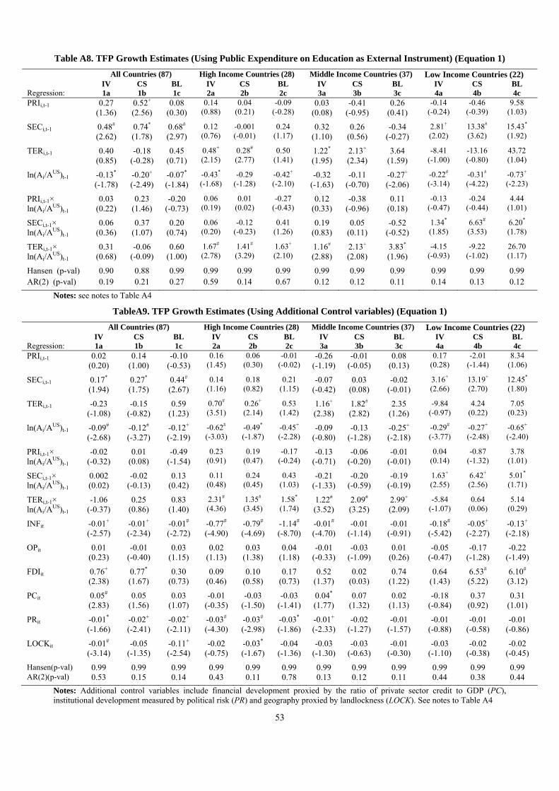
53

 

Table A8. TFP Growth Estimates (Using Public Expenditure on Education as External Instrument) (Equation 1)

All Countries (87) High Income Countries (28) Middle Income Countries (37) Low Income Countries (22) IV CS BL IV CS BL IV CS BL IV CS BL Regression: 1a 1b 1c 2a 2b 2c 3a 3b 3c 4a 4b 4c PRIi,t-1 0.27

(1.36) 0.52+ (2.56)

0.08 (0.30)

0.14 (0.88)

0.04 (0.21)

-0.09 (-0.28)

0.03 (0.08)

-0.41 (-0.95)

0.26 (0.41)

-0.14 (-0.24)

-0.46 (-0.39)

9.58 (1.03)

SECi,t-1 0.48# (2.62)

0.74* (1.78)

0.68# (2.97)

0.12 (0.76)

-0.001 (-0.01)

0.24 (1.17)

0.32 (1.10)

0.26 (0.56)

-0.34 (-0.27)

2.81+ (2.02)

13.38# (3.62)

15.43* (1.92)

TERi,t-1 0.40 (0.85)

-0.18 (-0.28)

0.45 (0.71)

0.48+ (2.15)

0.28# (2.77)

0.50 (1.41)

1.22* (1.95)

2.13+ (2.34)

3.64 (1.59)

-8.41 (-1.00)

-13.16 (-0.80)

43.72 (1.04)

ln(Ai/AUS)t-1 -0.13* (-1.78)

-0.20+ (-2.49)

-0.07* (-1.84)

-0.43* (-1.68)

-0.29 (-1.28)

-0.42+ (-2.10)

-0.32 (-1.63)

-0.11 (-0.70)

-0.27+ (-2.06)

-0.22# (-3.14)

-0.31# (-4.22)

-0.73+ (-2.23)

PRIi,t-1× ln(Ai/AUS)t-1

0.03 (0.22)

0.23 (1.46)

-0.20 (-0.73)

0.06 (0.19)

0.01 (0.02)

-0.27 (-0.43)

0.12 (0.33)

-0.38 (-0.96)

0.11 (0.18)

-0.13 (-0.47)

-0.24 (-0.44)

4.44 (1.01)

SECi,t-1× ln(Ai/AUS)t-1

0.06 (0.36)

0.37 (1.07)

0.20 (0.74)

0.06 (0.20)

-0.12 (-0.23)

0.41 (1.26)

0.19 (0.83)

0.05 (0.11)

-0.52 (-0.52)

1.34* (1.85)

6.63# (3.53)

6.20* (1.78)

TERi,t-1× ln(Ai/AUS)t-1

0.31 (0.68)

-0.06 (-0.09)

0.60 (1.00)

1.67#

(2.78) 1.41# (3.29)

1.63+ (2.10)

1.16# (2.88)

2.13+ (2.08)

3.83* (1.96)

-4.15 (-0.93)

-9.22 (-1.02)

26.70 (1.17)

Hansen (p-val) 0.90 0.88 0.99 0.99 0.99 0.99 0.99 0.99 0.99 0.99 0.99 0.99 AR(2) (p-val) 0.19 0.21 0.27 0.59 0.14 0.67 0.12 0.12 0.11 0.14 0.13 0.12

Notes: see notes to Table A4

TableA9. TFP Growth Estimates (Using Additional Control variables) (Equation 1)

All Countries (87) High Income Countries (28) Middle Income Countries (37) Low Income Countries (22) IV CS BL IV CS BL IV CS BL IV CS BL Regression: 1a 1b 1c 2a 2b 2c 3a 3b 3c 4a 4b 4c PRIi,t-1 0.02

(0.20) 0.14

(1.00) -0.10

(-0.53) 0.16

(1.45) 0.06

(0.30) -0.01

(-0.02) -0.26

(-1.19) -0.01

(-0.05) 0.08

(0.13) 0.17

(0.28) -2.01

(-1.44) 8.34

(1.06)

SECi,t-1 0.17* (1.94)

0.27* (1.75)

0.44# (2.67)

0.14 (1.16)

0.18 (0.82)

0.21 (1.15)

-0.07 (-0.42)

0.03 (0.08)

-0.02 (-0.01)

3.16+ (2.66)

13.19+ (2.70)

12.45* (1.80)

TERi,t-1 -0.23 (-1.08)

-0.15 (-0.82)

0.59 (1.23)

0.70# (3.51)

0.26+ (2.14)

0.53 (1.42)

1.16+ (2.38)

1.82# (2.82)

2.35 (1.26)

-9.84 (-0.97)

4.24 (0.22)

7.05 (0.23)

ln(Ai/AUS)t-1 -0.09# (-2.68)

-0.12# (-3.27)

-0.12+ (-2.19)

-0.62# (-3.03)

-0.49* (-1.87)

-0.45+ (-2.28)

-0.09 (-0.80)

-0.13 (-1.28)

-0.25+ (-2.18)

-0.29# (-3.77)

-0.27+ (-2.48)

-0.65+ (-2.40)

PRIi,t-1× ln(Ai/AUS)t-1

-0.02 (-0.32)

0.01 (0.08)

-0.49 (-1.54)

0.23 (0.91)

0.19 (0.47)

-0.17 (-0.24)

-0.13 (-0.71)

-0.06 (-0.20)

-0.01 (-0.01)

0.04 (0.14)

-0.87 (-1.32)

3.78 (1.01)

SECi,t-1× ln(Ai/AUS)t-1

0.002 (0.02)

-0.02 (-0.13)

0.13 (0.42)

0.11 (0.48)

0.24 (0.45)

0.43 (1.03)

-0.21 (-1.33)

-0.20 (-0.59)

-0.19 (-0.19)

1.63+ (2.55)

6.42+ (2.56)

5.01* (1.71)

TERi,t-1× ln(Ai/AUS)t-1

-1.06 (-0.37)

0.25 (0.86)

0.83 (1.40)

2.31#

(4.36) 1.35# (3.45)

1.58* (1.74)

1.22# (3.52)

2.09# (3.25)

2.99+ (2.09)

-5.84 (-1.07)

0.64 (0.06)

5.14 (0.29)

INFit -0.01+

(-2.57) -0.01+

(-2.34) -0.01#

(-2.72) -0.77#

(-4.90) -0.79#

(-4.69) -1.14#

(-8.70) -0.01#

(-4.70) -0.01

(-1.14) -0.01

(-0.91) -0.18#

(-5.42) -0.05+

(-2.27) -0.13+

(-2.18)

OPit 0.01 (0.23)

-0.01 (-0.40)

0.03 (1.15)

0.02 (1.13)

0.03 (1.38)

0.04 (1.18)

-0.01 (-0.33)

-0.03 (-1.09)

0.01 (0.26)

-0.05 (-0.47)

-0.17 (-1.28)

-0.22 (-1.49)

FDIit 0.76+ (2.38)

0.77* (1.67)

0.30 (0.73)

0.09 (0.46)

0.10 (0.58)

0.17 (0.73)

0.52 (1.37)

0.02 (0.03)

0.74 (1.22)

0.64 (1.43)

6.53# (5.22)

6.10# (3.12)

PCit 0.05# (2.83)

0.05 (1.56)

0.03 (1.07)

-0.01 (-0.35)

-0.03 (-1.50)

-0.03 (-1.41)

0.04* (1.77)

0.07 (1.32)

0.02 (1.13)

-0.18 (-0.84)

0.37 (0.92)

0.31 (1.01)

PRit -0.01* (-1.66)

-0.02+ (-2.41)

-0.02+ (-2.11)

-0.03# (-4.30)

-0.03# (-2.98)

-0.03* (-1.86)

-0.01+ (-2.33)

-0.02 (-1.27)

-0.01 (-1.57)

-0.01 (-0.88)

-0.01 (-0.58)

-0.01 (-0.86)

LOCKit -0.01# (-3.14)

-0.05 (-1.35)

-0.11+ (-2.54)

-0.02 (-0.75)

-0.03* (-1.67)

-0.04 (-1.36)

-0.03 (-1.30)

-0.03 (-0.63)

-0.01 (-0.30)

-0.03 (-1.10)

-0.02 (-0.38)

-0.02 (-0.45)

Hansen(p-val) 0.99 0.99 0.99 0.99 0.99 0.99 0.99 0.99 0.99 0.99 0.99 0.99 AR(2)(p-val) 0.53 0.15 0.14 0.43 0.11 0.78 0.13 0.12 0.11 0.44 0.38 0.44

Notes: Additional control variables include financial development proxied by the ratio of private sector credit to GDP (PC), institutional development measured by political risk (PR) and geography proxied by landlockness (LOCK). See notes to Table A4