HUMAN FACE DETECTION AND

RECOGNITION

A THESIS SUBMITTED IN PARALLEL FULFULMENT

OF THE REQUIREMENTS FOR THE DEGREE OF

Bachelor in Technology

In

Electronics and Communication Engineering

by

K Krishan Kumar Subudhi (107EC020)

And

Ramshankar Mishra(107EC004)

Department of Electronics and Communication Engineering

National Institute of Technology, Rourkela

2007-2011

ii

HUMAN FACE DETECTION AND

RECOGNITION

A THESIS SUBMITTED IN PARALLEL FULFULMENT

OF THE REQUIREMENTS FOR THE DEGREE OF

Bachelor in Technology

In

Electronics and Communication Engineering

by

K Krishan Kumar Subudhi (107EC020)

And

Ramshankar Mishra(107EC004)

Under the guidance of

Prof. S Meher

Department of Electronics and Communication Engineering

National Institute of Technology, Rourkela

2007-2011

iii

National Institute of Technology

Rourkela

CERTIFICATE

This is to certify that the thesis titled “Human Face Recognition and Detection”

submitted by K Krishan Kumar Subudhi (107EC020) and Ramshankar Mishra

(107EC004) in partial fulfilment for the requirements for the award of Bachelor

of Technology Degree in Electronics and Communication Engineering at

National Institute of Technology, Rourkela (Deemed University) is an authentic

work carried out by them under my supervision and guidance.

Date:

Prof. S Meher

Department of Electronics and

Communication Engineering

iv

ACKNOWLEDGEMENT

On the submission of our thesis report on “Human Face Detection and Recognition”, we

would like to extend our gratitude and sincere thanks to our supervisor Prof. S Meher,

Department of Electronics and Communication Engineering for his constant motivation and

support during the course of our work in the last one year. We truly appreciate and value his

esteemed guidance and encouragement from the beginning to the end of this thesis. We are

indebted to him for having helped us shape the problem and providing insights towards the

solution.

We want to thank all our teachers Prof. G.S.Rath, Prof.S.K.Patra, Prof.K.K.Mohapatra, Prof.

Poonam Singh, Prof.D.P.Acharya, Prof.S.K.Behera, Prof.Ajit Kumar Sahoo and Prof. Murthy

for providing a solid background for out studies and research thereafter. They have been great

sources of inspiration to us and we thank them from the bottom of our heart.

Above all, we would like to thank all our friends whose direct and indirect support helped us

complete our project in time. The thesis would have been impossible without their perpetual

moral support.

K Krishan Kumar Subudhi Ramshankar Mishra

Roll no.-107EC020 Roll no.-107EC004

v

Contents

HUMAN FACE DETECTION AND RECOGNITION ............................................................. i

CERTIFICATE ........................................................................................................................ iii

ACKNOWLEDGEMENT ........................................................................................................ iv

ABSTRACT ............................................................................................................................... 1

1 INTRODUCTION ............................................................................................................. 3

2 FACE RECOGNITION ..................................................................................................... 5

2.1 PRINCIPAL COMPONENT ANALYSIS (PCA) ...................................................... 5

2.1.1 The eigenface approach ............................................................................................ 6

2.1.2 Mathematical approach ............................................................................................. 8

2.2 Experimental analysis ................................................................................................. 9

2.2.1 Student database….................................................................................................... 9

2.2.2 Testing..................................................................................................................... 10

2.3 Advantages of PCA ................................................................................................... 12

2.4 Limitations of PCA ................................................................................................... 12

2.5 MPCALDA ............................................................................................................... 12

2.5.1 MPCA ..................................................................................................................... 12

2.5.2 LDA ........................................................................................................................ 13

2.5.3 Procedure ................................................................................................................ 14

2.5.4 Testing..................................................................................................................... 14

vi

2.5.5 Results ..................................................................................................................... 15

3 Face detection .................................................................................................................. 19

3.1 Introduction ............................................................................................................... 19

3.2 YCbCr model: ........................................................................................................... 19

3.2.1 Real time data ......................................................................................................... 20

3.3 Colour segmentation ................................................................................................. 21

3.4 Image segmentation................................................................................................... 22

3.5 Box formation ........................................................................................................... 25

3.6 Unwanted box rejection ............................................................................................ 25

3.6.1 Thresholding ........................................................................................................... 25

3.6.2 Box merging............................................................................................................ 26

3.6.3 Image matching ....................................................................................................... 26

3.7 Result ......................................................................................................................... 27

4 Conclusion ....................................................................................................................... 29

5 References ........................................................................................................................ 30

vii

Figures and Tables

Figure 1 : eigenfaces .................................................................................................................. 7

Figure 2 face database ................................................................................................................ 9

Figure 3 eigenfaces obtained ................................................................................................... 10

Figure 4 test image ................................................................................................................... 11

Figure 5 comparison with the database .................................................................................... 11

Figure 6 result after comparison .............................................................................................. 11

Figure 7 block diagram of MPCALDA ................................................................................... 14

Figure 8 representation of scatter matrices .............................................................................. 14

Figure 9 comparison between TSB and TSW.......................................................................... 15

Figure 10 fisher ration vs feature index ................................................................................... 16

Figure 11 fisher ration in descending order ............................................................................. 16

Figure 12 recognition using MPCALDA ................................................................................. 17

Figure 13 success rates............................................................................................................. 17

Figure 14 Cb vs Cr ................................................................................................................... 20

Figure 15 test image database for skin color analysis.............................................................. 20

Figure 16 histograms of Y, Cb and Cr values .......................................................................... 21

Figure 17 test image for face detection .................................................................................... 21

Figure 18 image after passing through YCbCr filter ............................................................... 22

Figure 19 black isolated hole rejection .................................................................................... 22

Figure 20 white isolated holes less than small area rejection .................................................. 23

Figure 21 edges detected by Roberts cross operator ................................................................ 23

Figure 22 integration of two images edge+filtered .................................................................. 24

Figure 23 second black isolated hole rejection ........................................................................ 24

viii

Figure 24 small areas less than minimum area rejection ......................................................... 24

Figure 25 initial box formation ................................................................................................ 25

Figure 26 thresholding ............................................................................................................. 25

Figure 27 box merging ............................................................................................................. 26

Figure 28mean eigen face Figure 29 eigenfaces ......................................................... 26

Figure 30 different sized eigen face ......................................................................................... 27

Figure 31 histogram of correlated values................................................................................. 27

Figure 32 final detected image ................................................................................................. 27

Figure 33 detection with a coloured background ..................................................................... 28

Figure 34 another image .......................................................................................................... 28

Figure 35 better result .............................................................................................................. 29

Table 1 comparison between PCA and MPCALDA ............................................................... 17

Table 2 table of results ............................................................................................................. 29

1

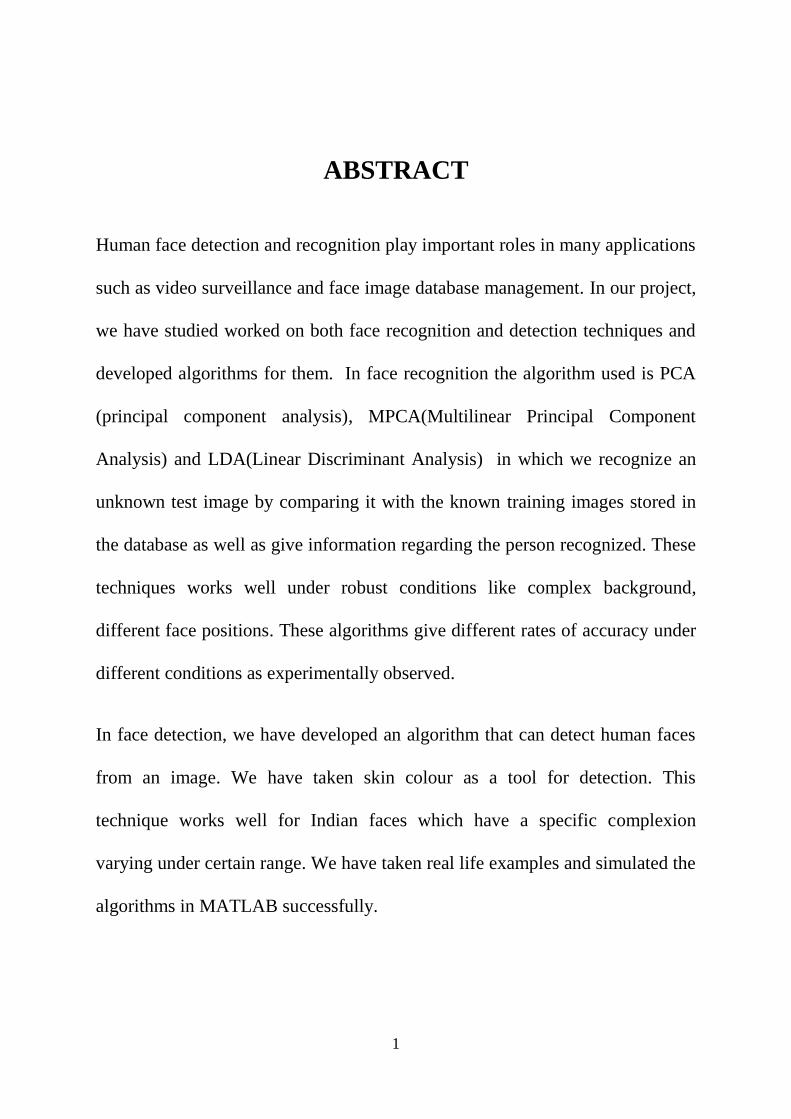
ABSTRACT

Human face detection and recognition play important roles in many applications

such as video surveillance and face image database management. In our project,

we have studied worked on both face recognition and detection techniques and

developed algorithms for them. In face recognition the algorithm used is PCA

(principal component analysis), MPCA(Multilinear Principal Component

Analysis) and LDA(Linear Discriminant Analysis) in which we recognize an

unknown test image by comparing it with the known training images stored in

the database as well as give information regarding the person recognized. These

techniques works well under robust conditions like complex background,

different face positions. These algorithms give different rates of accuracy under

different conditions as experimentally observed.

In face detection, we have developed an algorithm that can detect human faces

from an image. We have taken skin colour as a tool for detection. This

technique works well for Indian faces which have a specific complexion

varying under certain range. We have taken real life examples and simulated the

algorithms in MATLAB successfully.

2

CHAPTER-1 INTRODUCTION

3

1 INTRODUCTION

The face is our primary focus of attention in social life playing an important role in

conveying identity and emotions. We can recognize a number of faces learned throughout our

lifespan and identify faces at a glance even after years of separation. This skill is quite robust

despite of large variations in visual stimulus due to changing condition, aging and distractions

such as beard, glasses or changes in hairstyle.

Computational models of face recognition are interesting because they can contribute not

only to theoretical knowledge but also to practical applications. Computers that detect and

recognize faces could be applied to a wide variety of tasks including criminal identification,

security system, image and film processing, identity verification, tagging purposes and

human-computer interaction. Unfortunately, developing a computational model of face

detection and recognition is quite difficult because faces are complex, multidimensional and

meaningful visual stimuli.

Face detection is used in many places now a days especially the websites hosting images like

picassa, photobucket and facebook. The automatically tagging feature adds a new dimension

to sharing pictures among the people who are in the picture and also gives the idea to other

people about who the person is in the image. In our project, we have studied and

implemented a pretty simple but very effective face detection algorithm which takes human

skin colour into account.

Our aim, which we believe we have reached, was to develop a method of face recognition

that is fast, robust, reasonably simple and accurate with a relatively simple and easy to

understand algorithms and techniques. The examples provided in this thesis are real-time and

taken from our own surroundings.

4

CHAPTER 2 FACE RECOGNITION

5

2 FACE RECOGNITION

The face recognition algorithms used here are Principal Component Analysis(PCA),

Multilinear Principal Component Analysis (MPCA) and Linear Discriminant Analysis(LDA).

Every algorithm has its own advantage. While PCA is the most simple and fast algorithm,

MPCA and LDA which have been applied together as a single algorithm named MPCALDA

provide better results under complex circumstances like face position, luminance variation

etc. Each of them have been discussed one by one below.

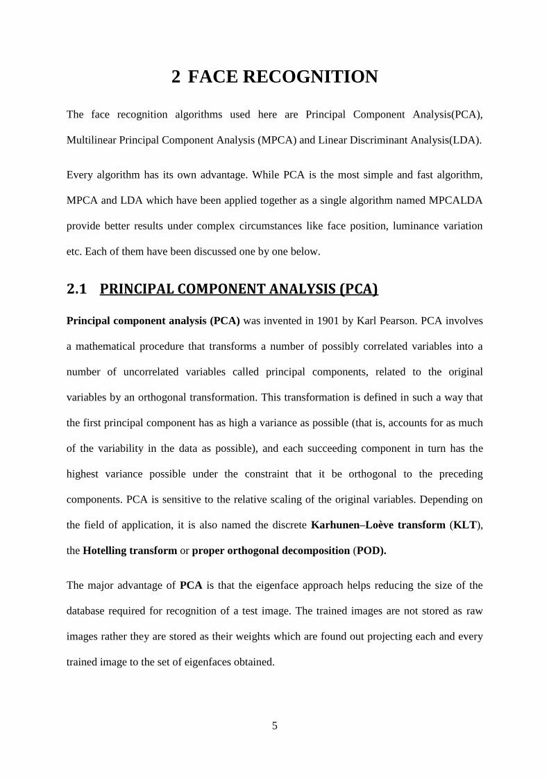
2.1 PRINCIPAL COMPONENT ANALYSIS (PCA)

Principal component analysis (PCA) was invented in 1901 by Karl Pearson. PCA involves

a mathematical procedure that transforms a number of possibly correlated variables into a

number of uncorrelated variables called principal components, related to the original

variables by an orthogonal transformation. This transformation is defined in such a way that

the first principal component has as high a variance as possible (that is, accounts for as much

of the variability in the data as possible), and each succeeding component in turn has the

highest variance possible under the constraint that it be orthogonal to the preceding

components. PCA is sensitive to the relative scaling of the original variables. Depending on

the field of application, it is also named the discrete Karhunen–Loève transform (KLT),

the Hotelling transform or proper orthogonal decomposition (POD).

The major advantage of PCA is that the eigenface approach helps reducing the size of the

database required for recognition of a test image. The trained images are not stored as raw

images rather they are stored as their weights which are found out projecting each and every

trained image to the set of eigenfaces obtained.

6

2.1.1 The eigenface approach

In the language of information theory, the relevant information in a face needs to be

extracted, encoded efficiently and one face encoding is compared with the similarly encoded

database. The trick behind extracting such kind of information is to capture as many

variations as possible from the set of training images.

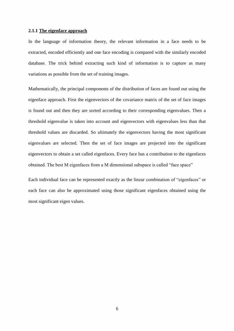
Mathematically, the principal components of the distribution of faces are found out using the

eigenface approach. First the eigenvectors of the covariance matrix of the set of face images

is found out and then they are sorted according to their corresponding eigenvalues. Then a

threshold eigenvalue is taken into account and eigenvectors with eigenvalues less than that

threshold values are discarded. So ultimately the eigenvectors having the most significant

eigenvalues are selected. Then the set of face images are projected into the significant

eigenvectors to obtain a set called eigenfaces. Every face has a contribution to the eigenfaces

obtained. The best M eigenfaces from a M dimensional subspace is called “face space”

Each individual face can be represented exactly as the linear combination of “eigenfaces” or

each face can also be approximated using those significant eigenfaces obtained using the

most significant eigen values.

7

Figure 1 : eigenfaces

Now the test image subjected to recognition is also projected to the face space and then the

weights corresponding to each eigenface are found out. Also the weights of all the training

images are found out and stored. Now the weights of the test image is compared to the set of

weights of the training images and the best possible match is found out. The comparison is

done using the “Euclidean distance” measurement. Minimum the distance is the maximum

is the match.

The approach to face recognition involves the following initialisation operations:

1. Acquire an initial set of N face images (training images).

2. Calculate the eigenface from the training set keeping only the M images that

correspond to the highest eigenvalues. These M images define the “facespace”. As

8

new faces are encountered, the “eigenfaces” can be updated or recalculated

accordingly.

3. Calculate the corresponding distribution in M dimensional weight space for each

known individual by projecting their face images onto the “face space”.

4. Calculate a set of weights projecting the input image to the M “eigenfaces”.

5. Determine whether the image is a face or not by checking the closeness of the image

to the “face space”.

6. If it is close enough, classify, the weight pattern as either a known person or as an

unknown based on the Euclidean distance measured.

7. If it is close enough then cite the recognition successful and provide relevant

information about the recognised face form the database which contains information

about the faces.

2.1.2 Mathematical approach

Let Г1, Г2, …, Гm be the set of train images.

Average face of set can be defined as ∑

Each face differs from the average by the vector Фi = Гi – ψ

when subjected to PCA, this large set of vectors seeks a set of M orthogonal vectors Un,

which best describes the distribution of data.

The kth vector Uk is chosen such that

λk= ∑

T * Фn]

2

is maximum, subject to (Ul)T UK = δlk = {

1, if l=k 0, otherwise

9

The vector Uk and scalar λk are the eigenvectors and eigenvalues respectively of the

covariance matrix

C = ∑

T

= AAT

Where the matrix A= [Ф1 Ф2 ….. ФM].

2.2 Experimental analysis

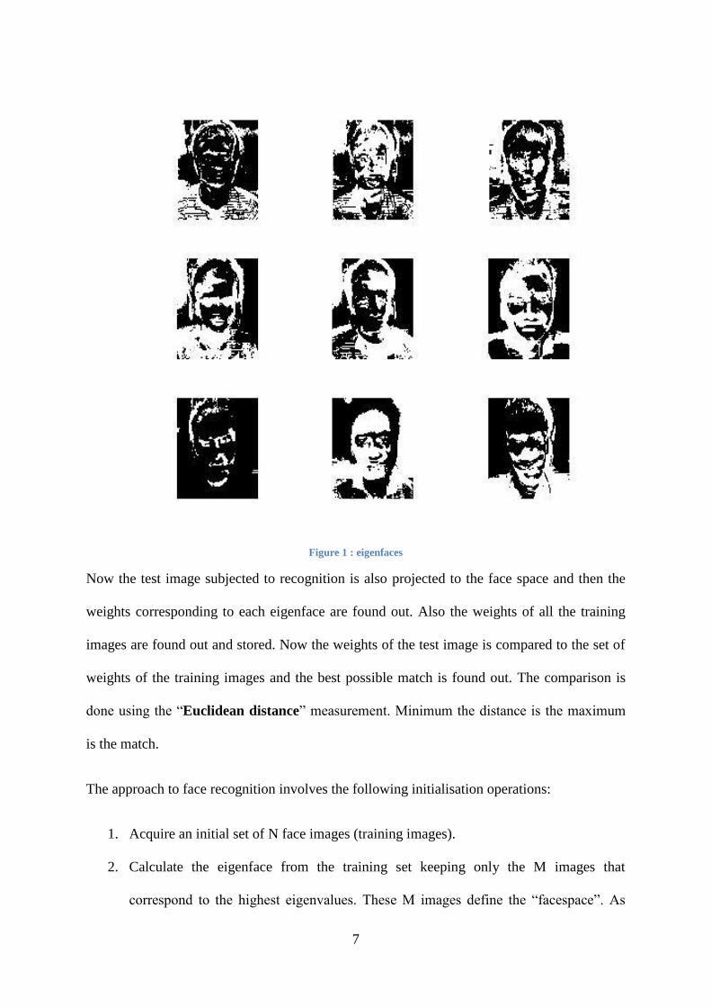
We created a student database of NIT Rourkela which contains their photographs and

information (name, age, roll no).

2.2.1 Student database…..

Figure 2 face database

10

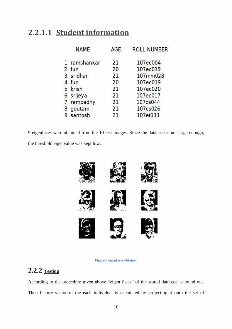
2.2.1.1 Student information

9 eigenfaces were obtained from the 10 test images. Since the database is not large enough,

the threshold eigenvalue was kept low.

Figure 3 eigenfaces obtained

2.2.2 Testing

According to the procedure given above “eigen faces” of the stored database is found out.

Then feature vector of the each individual is calculated by projecting it onto the set of

11

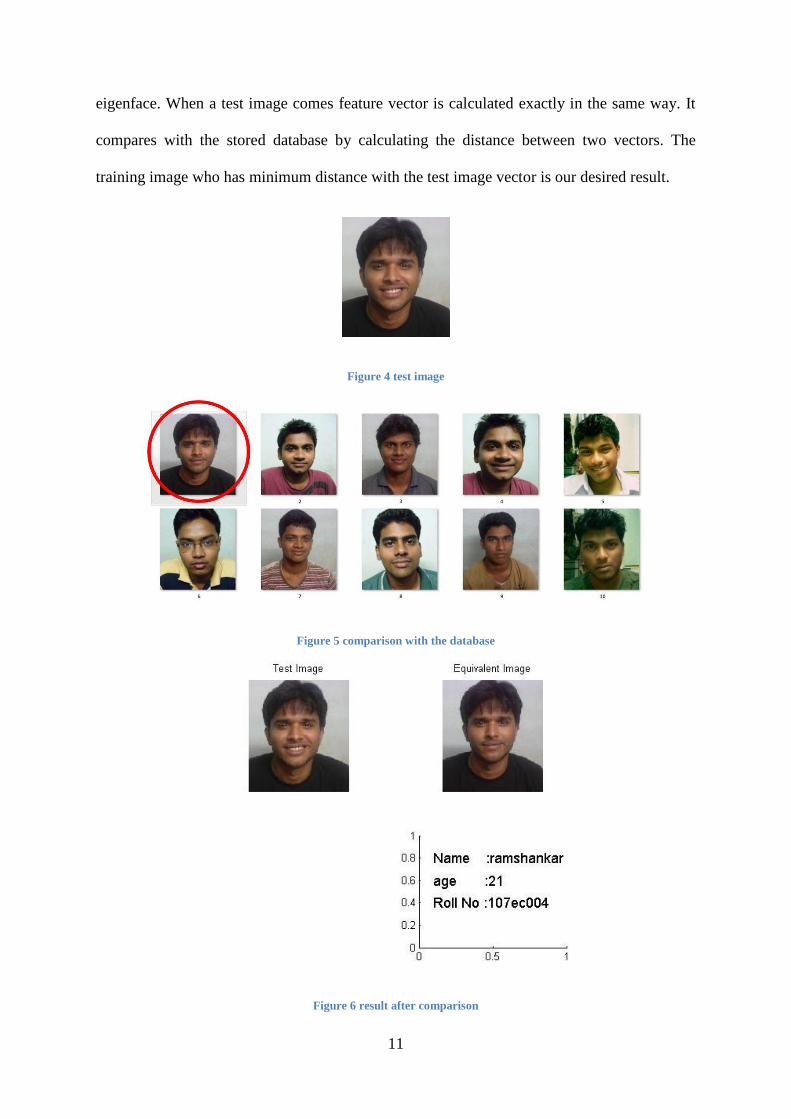
eigenface. When a test image comes feature vector is calculated exactly in the same way. It

compares with the stored database by calculating the distance between two vectors. The

training image who has minimum distance with the test image vector is our desired result.

Figure 4 test image

Figure 5 comparison with the database

Figure 6 result after comparison

12

2.3 Advantages of PCA

1. It’s the simplest approach which can be used for data compression and face

recognition.

2. Operates at a faster rate.

2.4 Limitations of PCA

1. Requires full frontal display of faces

2. Not sensitive to lighting conditions, position of faces.

3. Considers every face in the database as a different image. Faces of the same person

are not classified in classes.

A better approach was studied and used to compensate these limitations which are called

MPCALDA. While MPCA considers the different variations in images, LDA classifies the

images according to same or different person.

2.5 MPCALDA

2.5.1 MPCA

Multilinear Principal Component Analysis (MPCA) is the extension of PCA that uses

multilinear algebra and proficient of learning the interactions of the multiple factors like

different viewpoints, different lighting conditions, different expressions etc.

In PCA the aim was to reduce the dimensionality of the images. For example a 20x32x30

dataset was converted to 640x30 that is images are converted to 1D matrices and then the

eigenfaces were found out out of them. But this approach ignores all other dimensions of an

image as an image of size 20x32 speaks of a lot of dimensions in a face and 1D vectorizing

13

doesn’t take advantage of all those features. Therefore a dimensionality reduction technique

operating directly on the tensor object rather than its 1D vectorized version is applied here.

The basic idea behind consideration of different dimensions can be explained by the below

formula.

Where Yi = output , Xi = input, U(n)

= transformation vectors

The approach is similar to PCA in which the features representing a face are reduced by

eigenface approach. While in PCA only one transformation vector was used, in MPCA N

number of different transformation vectors representing the different dimensionality of the

face images are applied.

2.5.2 LDA

LDA which is known as Linear Discriminant Analysis is a computational scheme for

evaluating the significance of different facial attributes in terms of their discrimination

power. The database is divided into a number of classes each class contains a set of images of

the same person in different viewing conditions like different frontal views, facial expression,

different lighting and background conditions and images with or without glasses etc. It is also

assumed that all images consist of only the face regions and are of same size.

By defining all the face images of the same person in one class and faces of other people in

different classes we can establish a model for performing cluster separation analysis. We

have achieved this objective by defining two terms named “between class scatter matrix” and

“within class scatter matrix”. The database used here is a FERET database which is a

reference database for the testing of our studied algorithm.

14

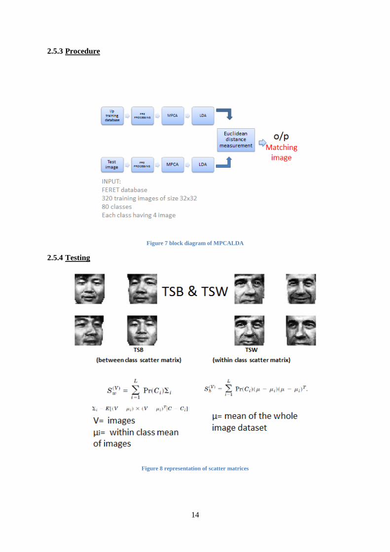
2.5.3 Procedure

Figure 7 block diagram of MPCALDA

2.5.4 Testing

Figure 8 representation of scatter matrices

15

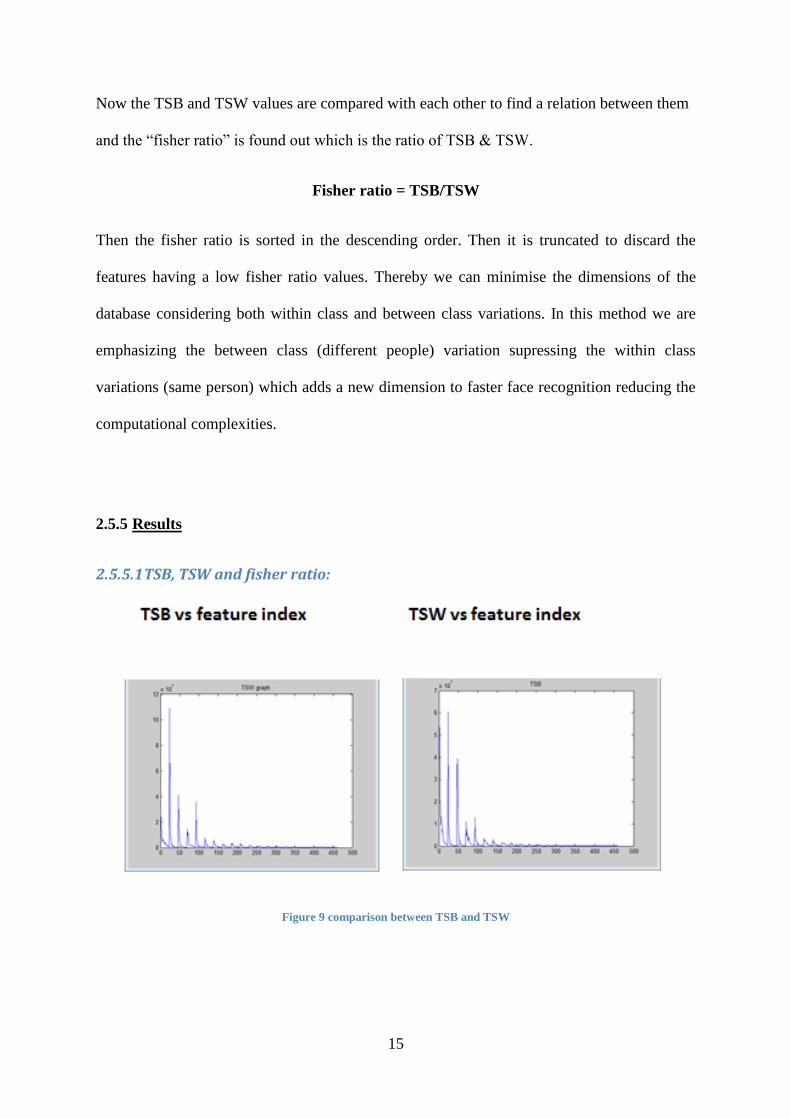
Now the TSB and TSW values are compared with each other to find a relation between them

and the “fisher ratio” is found out which is the ratio of TSB & TSW.

Fisher ratio = TSB/TSW

Then the fisher ratio is sorted in the descending order. Then it is truncated to discard the

features having a low fisher ratio values. Thereby we can minimise the dimensions of the

database considering both within class and between class variations. In this method we are

emphasizing the between class (different people) variation supressing the within class

variations (same person) which adds a new dimension to faster face recognition reducing the

computational complexities.

2.5.5 Results

2.5.5.1 TSB, TSW and fisher ratio:

Figure 9 comparison between TSB and TSW

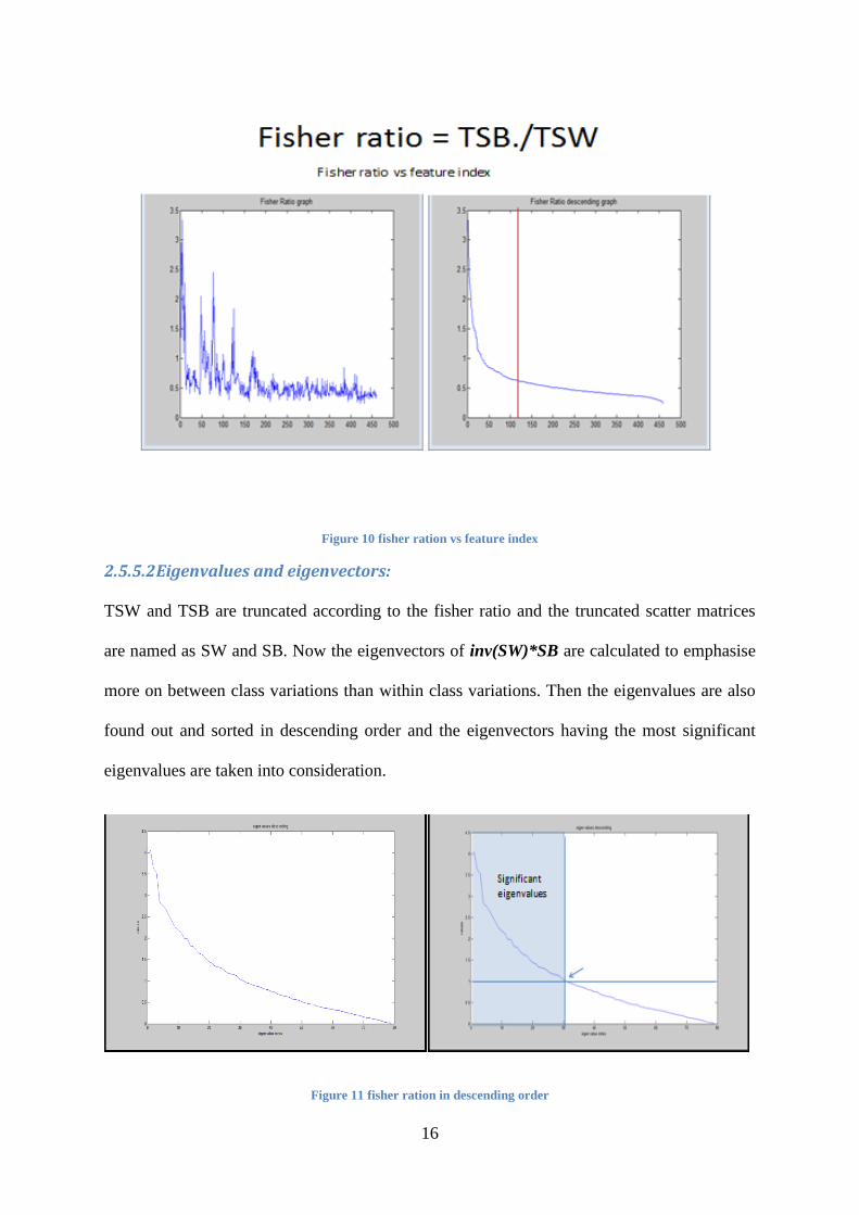
16

Figure 10 fisher ration vs feature index

2.5.5.2 Eigenvalues and eigenvectors:

TSW and TSB are truncated according to the fisher ratio and the truncated scatter matrices

are named as SW and SB. Now the eigenvectors of inv(SW)*SB are calculated to emphasise

more on between class variations than within class variations. Then the eigenvalues are also

found out and sorted in descending order and the eigenvectors having the most significant

eigenvalues are taken into consideration.

Figure 11 fisher ration in descending order

17

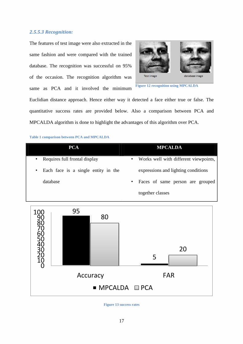
2.5.5.3 Recognition:

The features of test image were also extracted in the

same fashion and were compared with the trained

database. The recognition was successful on 95%

of the occasion. The recognition algorithm was

same as PCA and it involved the minimum

Euclidian distance approach. Hence either way it detected a face either true or false. The

quantitative success rates are provided below. Also a comparison between PCA and

MPCALDA algorithm is done to highlight the advantages of this algorithm over PCA.

Table 1 comparison between PCA and MPCALDA

PCA MPCALDA

• Requires full frontal display

• Each face is a single entity in the

database

• Works well with different viewpoints,

expressions and lighting conditions

• Faces of same person are grouped

together classes

Figure 13 success rates

95

5

80

20

0102030405060708090

100

Accuracy FAR

MPCALDA PCA

Figure 12 recognition using MPCALDA

18

Chapter 3 Face detection

19

3 Face detection

3.1 Introduction

Face detection is the first step of face recognition as it automatically detects a face from a

complex background to which the face recognition algorithm can be applied. But detection

itself involves many complexities such as background, poses, illumination etc.

There are many approaches for face detection such as, colour based, feature based (mouth,

eyes, nose), neural network. The approach studied and applied in this thesis is the skin colour

based approach. The algorithm is pretty robust as the faces of many people can be detected at

once from an image consisting of a group of people. The model to detect skin colour used

here is the YCbCr model.

The different steps of this face detection algorithm can be explained as below.

3.2 YCbCr model:

YCbCr or Y’CbCr is a family of color space used generally in digital image processing. Y is

the luminance, Y’ is the luma component while Cb and Cr are the blue difference and red

difference of the chroma component. YCbCr is not an actual colour space, it is just a way of

encoding the RGB colour space. YCbCr values can only be obtained only if the original RGB

information of the image are available.

Y = 0.299R + 0.587G + 0.114B

Cb = -0.169R - 0.332G + 0.500B

Cr = 0.500R - 0.419G - 0.081B

20

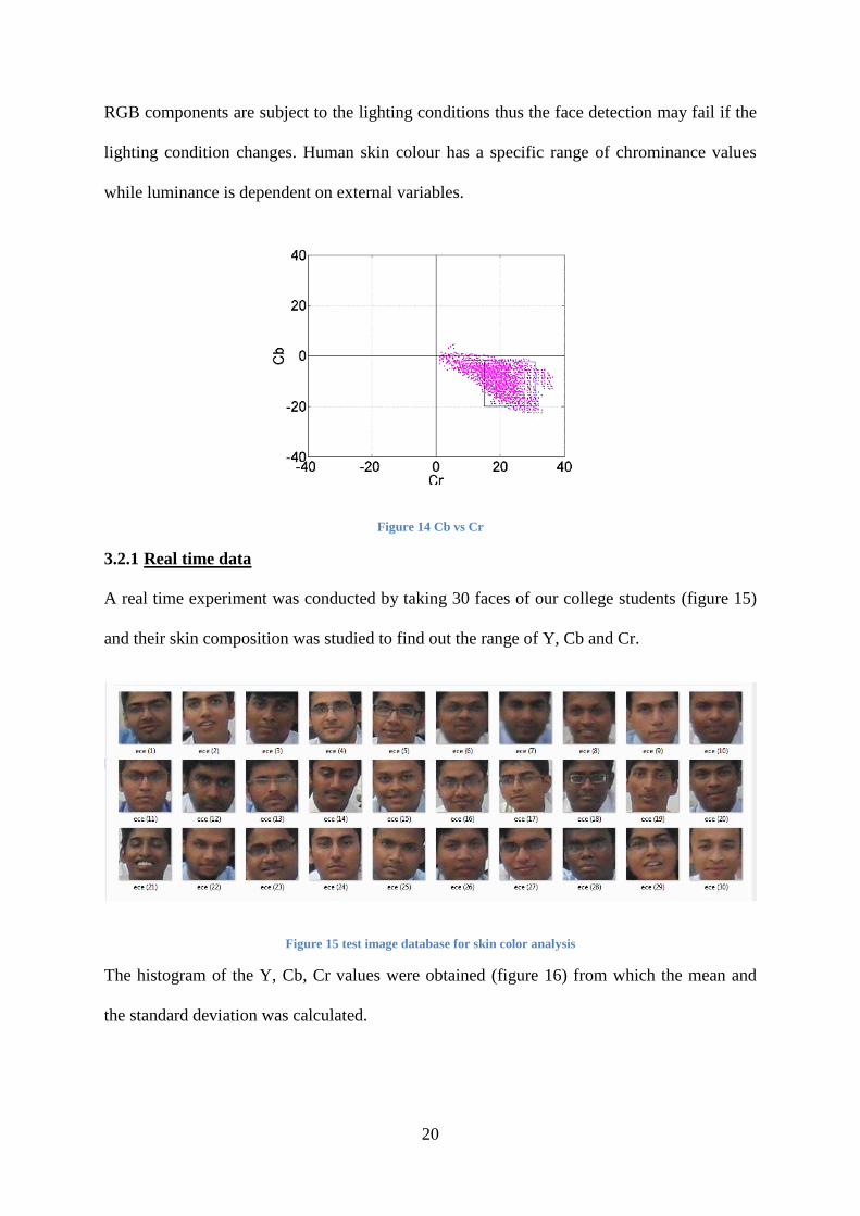
RGB components are subject to the lighting conditions thus the face detection may fail if the

lighting condition changes. Human skin colour has a specific range of chrominance values

while luminance is dependent on external variables.

Figure 14 Cb vs Cr

3.2.1 Real time data

A real time experiment was conducted by taking 30 faces of our college students (figure 15)

and their skin composition was studied to find out the range of Y, Cb and Cr.

Figure 15 test image database for skin color analysis

The histogram of the Y, Cb, Cr values were obtained (figure 16) from which the mean and

the standard deviation was calculated.

21

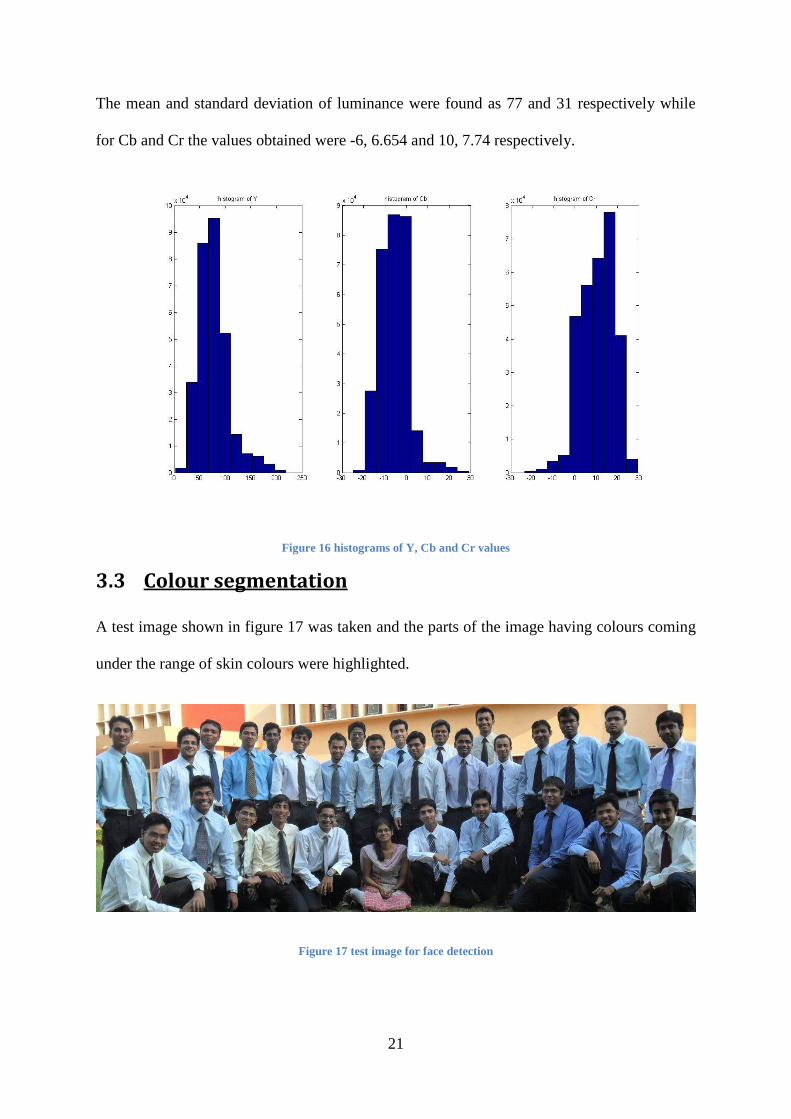
The mean and standard deviation of luminance were found as 77 and 31 respectively while

for Cb and Cr the values obtained were -6, 6.654 and 10, 7.74 respectively.

Figure 16 histograms of Y, Cb and Cr values

3.3 Colour segmentation

A test image shown in figure 17 was taken and the parts of the image having colours coming

under the range of skin colours were highlighted.

Figure 17 test image for face detection

22

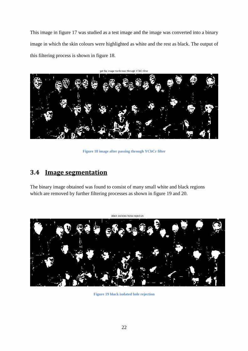
This image in figure 17 was studied as a test image and the image was converted into a binary

image in which the skin colours were highlighted as white and the rest as black. The output of

this filtering process is shown in figure 18.

Figure 18 image after passing through YCbCr filter

3.4 Image segmentation

The binary image obtained was found to consist of many small white and black regions

which are removed by further filtering processes as shown in figure 19 and 20.

Figure 19 black isolated hole rejection

23

Figure 20 white isolated holes less than small area rejection

As some face regions may be integrated with other face regions, they need to be separated.

For that purpose, Robert Cross Edge detection Algorithm is used. The Robert algorithm finds

the edges or the first gradient of the test image.

Figure 21 edges detected by Roberts cross operator

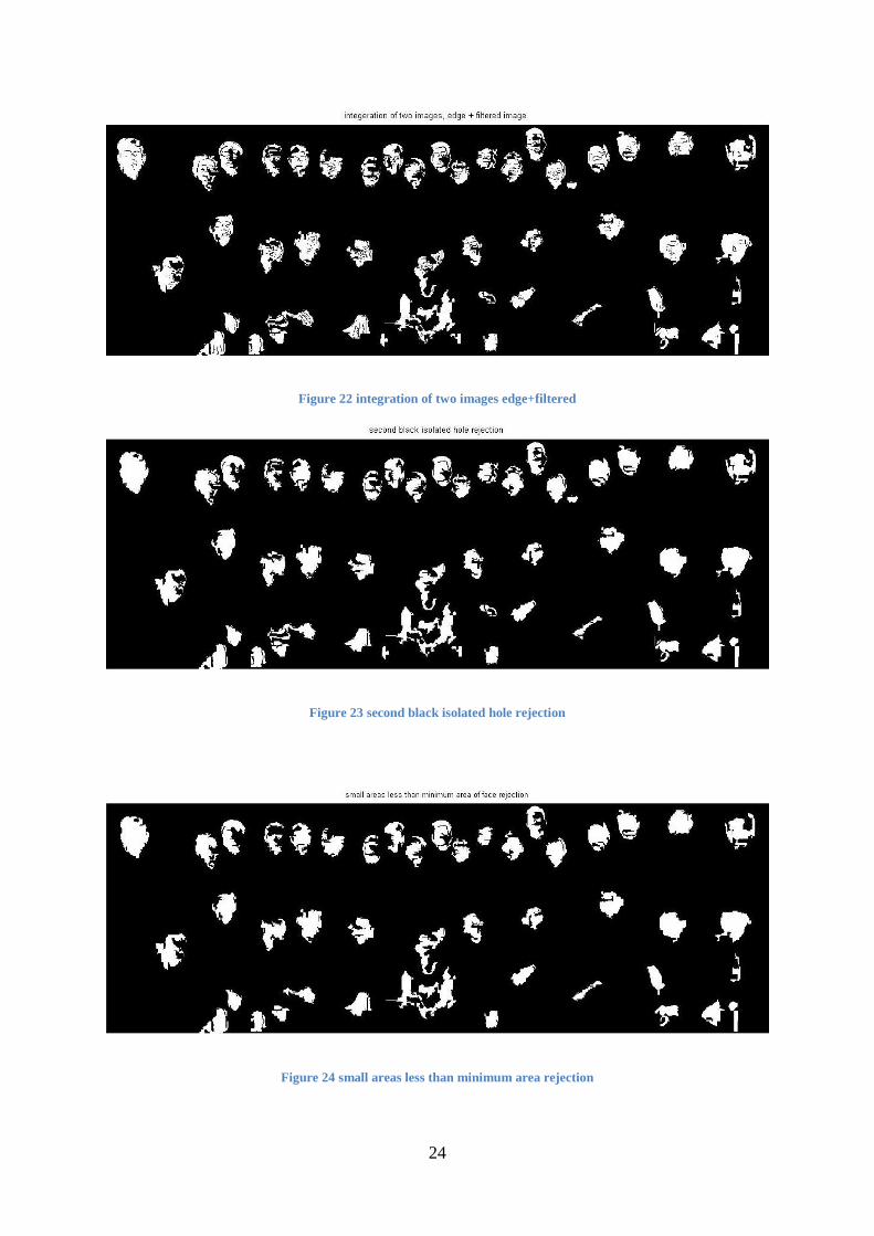
Now the filtered image and the edge images both are integrated to remove relatively small

white and black areas and the the image is again passed through the filters to obtain the final

filtered binary image. Figure 24 shows the final binary image.

24

Figure 22 integration of two images edge+filtered

Figure 23 second black isolated hole rejection

Figure 24 small areas less than minimum area rejection

25

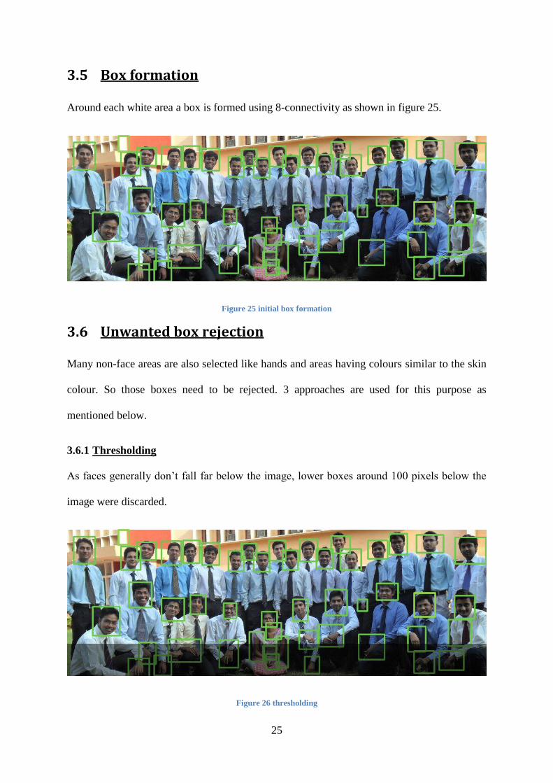
3.5 Box formation

Around each white area a box is formed using 8-connectivity as shown in figure 25.

Figure 25 initial box formation

3.6 Unwanted box rejection

Many non-face areas are also selected like hands and areas having colours similar to the skin

colour. So those boxes need to be rejected. 3 approaches are used for this purpose as

mentioned below.

3.6.1 Thresholding

As faces generally don’t fall far below the image, lower boxes around 100 pixels below the

image were discarded.

Figure 26 thresholding

26

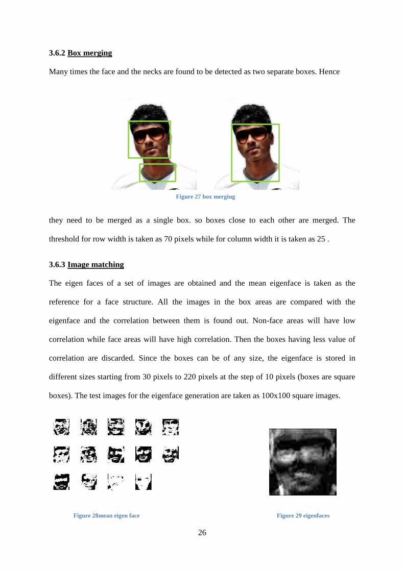
3.6.2 Box merging

Many times the face and the necks are found to be detected as two separate boxes. Hence

they need to be merged as a single box. so boxes close to each other are merged. The

threshold for row width is taken as 70 pixels while for column width it is taken as 25 .

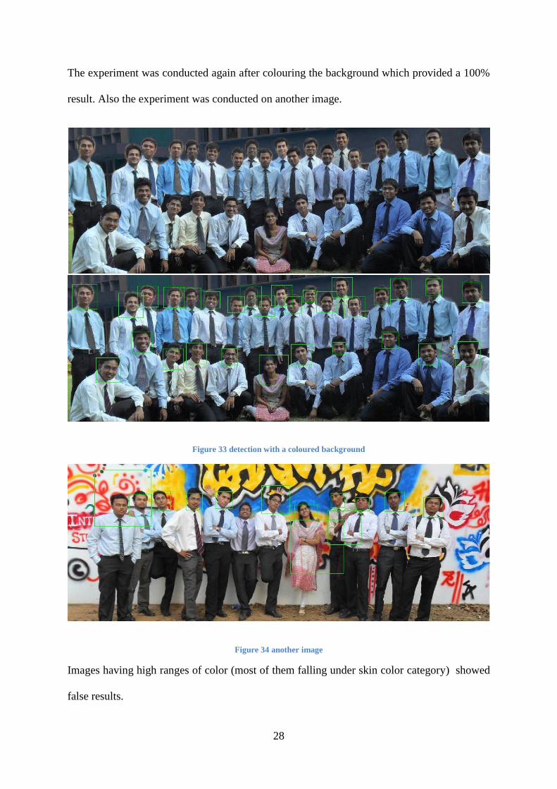
3.6.3 Image matching

The eigen faces of a set of images are obtained and the mean eigenface is taken as the

reference for a face structure. All the images in the box areas are compared with the

eigenface and the correlation between them is found out. Non-face areas will have low

correlation while face areas will have high correlation. Then the boxes having less value of

correlation are discarded. Since the boxes can be of any size, the eigenface is stored in

different sizes starting from 30 pixels to 220 pixels at the step of 10 pixels (boxes are square

boxes). The test images for the eigenface generation are taken as 100x100 square images.

Figure 28mean eigen face Figure 29 eigenfaces

Figure 27 box merging

27

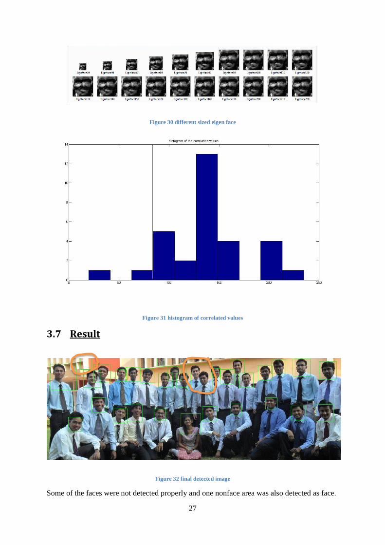
Figure 30 different sized eigen face

Figure 31 histogram of correlated values

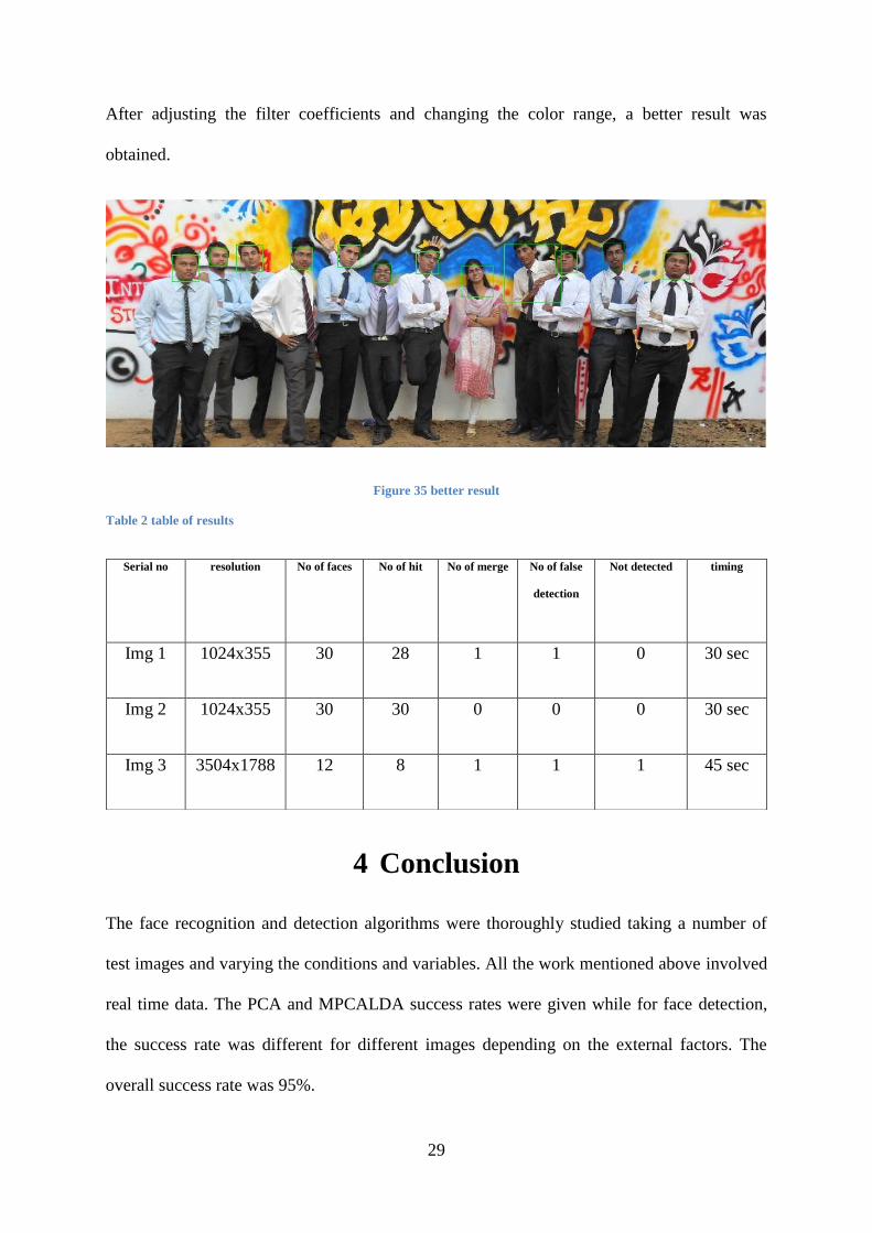
3.7 Result

Figure 32 final detected image

Some of the faces were not detected properly and one nonface area was also detected as face.

28

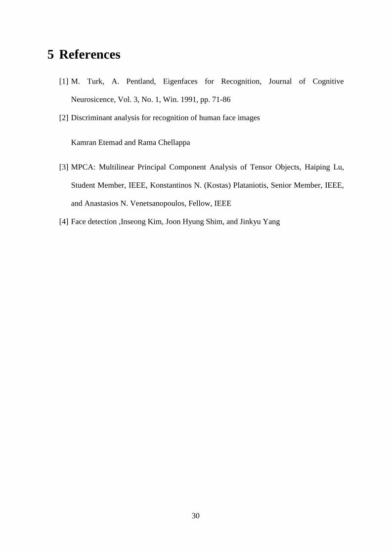
The experiment was conducted again after colouring the background which provided a 100%

result. Also the experiment was conducted on another image.

Figure 33 detection with a coloured background

Figure 34 another image

Images having high ranges of color (most of them falling under skin color category) showed

false results.

29

After adjusting the filter coefficients and changing the color range, a better result was

obtained.

Figure 35 better result

Table 2 table of results

4 Conclusion

The face recognition and detection algorithms were thoroughly studied taking a number of

test images and varying the conditions and variables. All the work mentioned above involved

real time data. The PCA and MPCALDA success rates were given while for face detection,

the success rate was different for different images depending on the external factors. The

overall success rate was 95%.

Serial no resolution No of faces No of hit No of merge No of false

detection

Not detected timing

Img 1 1024x355 30 28 1 1 0 30 sec

Img 2 1024x355 30 30 0 0 0 30 sec

Img 3 3504x1788 12 8 1 1 1 45 sec

30

5 References

[1] M. Turk, A. Pentland, Eigenfaces for Recognition, Journal of Cognitive

Neurosicence, Vol. 3, No. 1, Win. 1991, pp. 71-86

[2] Discriminant analysis for recognition of human face images

Kamran Etemad and Rama Chellappa

[3] MPCA: Multilinear Principal Component Analysis of Tensor Objects, Haiping Lu,

Student Member, IEEE, Konstantinos N. (Kostas) Plataniotis, Senior Member, IEEE,

and Anastasios N. Venetsanopoulos, Fellow, IEEE

[4] Face detection ,Inseong Kim, Joon Hyung Shim, and Jinkyu Yang