Embed Size (px)
Citation preview
Huygens’ Principle, Integrable PDEs, and Solitons
Jorge P. Zubelli
July 20, 2004
http://www.impa.br/ zubelli/ download:http://www.impa.br/˜zubelli/
Thanks: Prof. Marco Calahorrano
Joint work with Fabio Chalub - U. Lisboa
Overview
• Free Space Waves in (2+1) Dimensions × (3+1) Dimensions
Overview
• Free Space Waves in (2+1) Dimensions × (3+1) Dimensions
• Huygens’ principle in Hadamard’s sense
Overview
• Free Space Waves in (2+1) Dimensions × (3+1) Dimensions
• Huygens’ principle in Hadamard’s sense
• The Hadamard conjecture
Overview
• Free Space Waves in (2+1) Dimensions × (3+1) Dimensions
• Huygens’ principle in Hadamard’s sense
• The Hadamard conjecture
• Calogero-Moser Systems
Overview
• Free Space Waves in (2+1) Dimensions × (3+1) Dimensions
• Huygens’ principle in Hadamard’s sense
• The Hadamard conjecture
• Calogero-Moser Systems
• Solitons - KdV, KP, and Friends
Overview
• Free Space Waves in (2+1) Dimensions × (3+1) Dimensions
• Huygens’ principle in Hadamard’s sense
• The Hadamard conjecture
• Calogero-Moser Systems
• Solitons - KdV, KP, and Friends
• Huygens for Dirac Systems

Overview
• Free Space Waves in (2+1) Dimensions × (3+1) Dimensions
• Huygens’ principle in Hadamard’s sense
• The Hadamard conjecture
• Calogero-Moser Systems
• Solitons - KdV, KP, and Friends
• Huygens for Dirac Systems
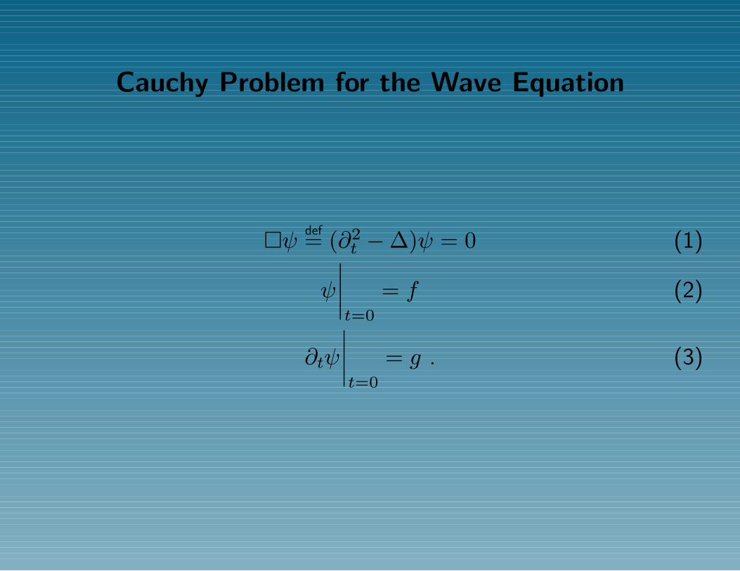
Cauchy Problem for the Wave Equation
ψdef= (∂2
t −∆)ψ = 0 (1)
ψ
∣∣∣∣t=0
= f (2)
∂tψ
∣∣∣∣t=0
= g . (3)
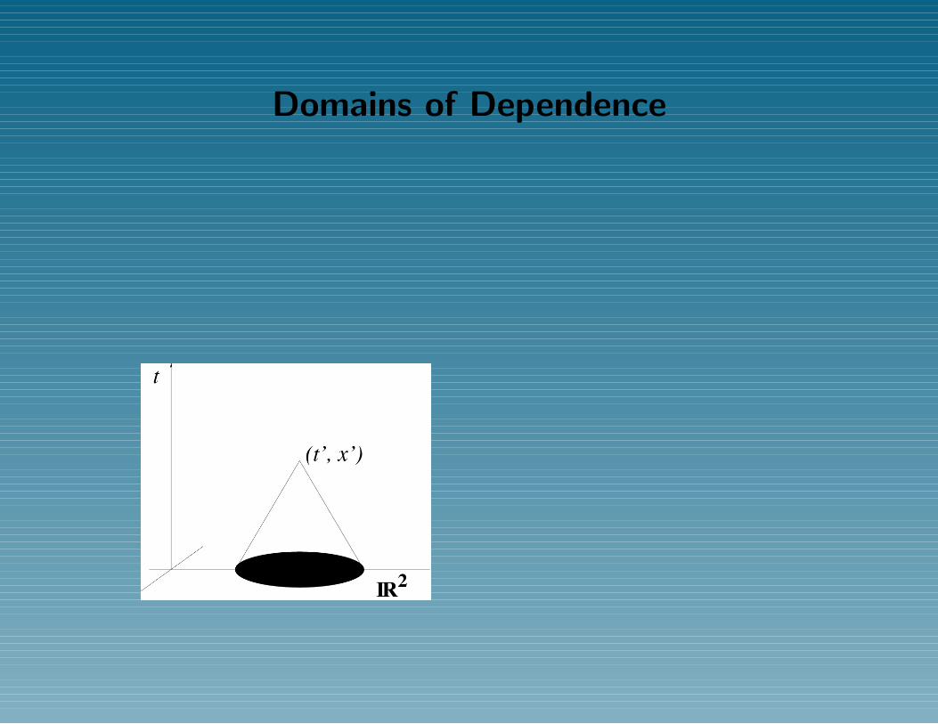
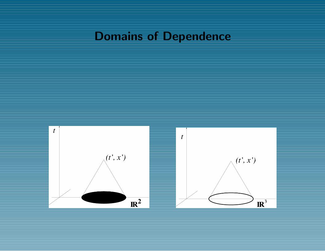
Domains of Dependence

Domains of Dependence
Domains of Dependence
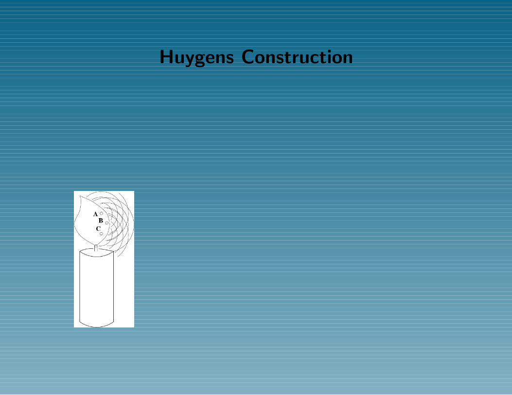
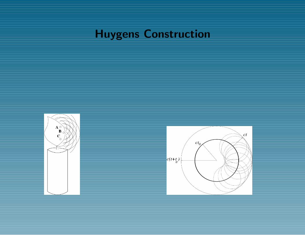
Huygens Construction

Huygens Construction
Huygens Construction
Hadamard’s Approach Huygens’ Property
(A) “Major Premise”
The action of phenomena produced at the instant t = 0 on
the state of matter at the later time t = t0 takes place by the
mediation of every intermediary instant t = t′, i.e., (assuming
0 < t′ < t0), . . .
Hadamard’s Approach Huygens’ Property
(A) “Major Premise”
The action of phenomena produced at the instant t = 0 on
the state of matter at the later time t = t0 takes place by the
mediation of every intermediary instant t = t′, i.e., (assuming
0 < t′ < t0), . . .
(B) “Minor Premise”
If we produce a luminous disturbance localized in a
neighborhood of 0, its effect after an elapsed time t0 will
be localized in a neighborhood of the sphere centered at 0 with
radius ct0.
be localized in a neighborhood of the sphere centered at 0 with
radius ct0.
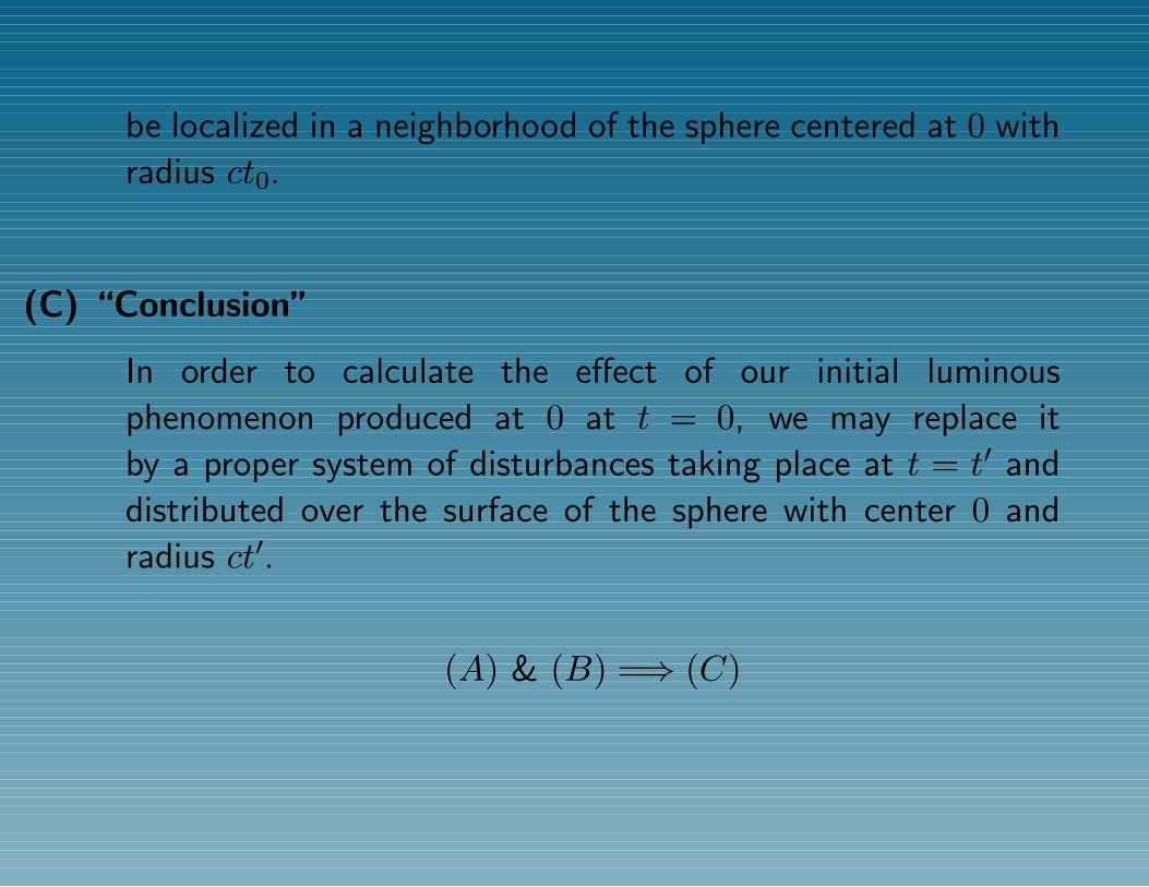
(C) “Conclusion”
In order to calculate the effect of our initial luminous
phenomenon produced at 0 at t = 0, we may replace it
by a proper system of disturbances taking place at t = t′ and
distributed over the surface of the sphere with center 0 and
radius ct′.

be localized in a neighborhood of the sphere centered at 0 with
radius ct0.
(C) “Conclusion”
In order to calculate the effect of our initial luminous
phenomenon produced at 0 at t = 0, we may replace it
by a proper system of disturbances taking place at t = t′ and
distributed over the surface of the sphere with center 0 and
radius ct′.
(A) & (B) =⇒ (C)

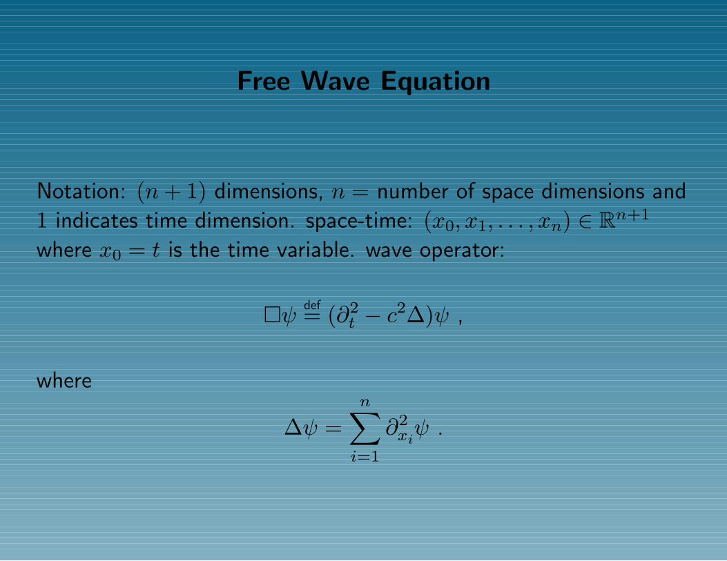
Free Wave Equation
Notation: (n+ 1) dimensions, n = number of space dimensions and
1 indicates time dimension. space-time: (x0, x1, . . . , xn) ∈ Rn+1
where x0 = t is the time variable. wave operator:
ψdef= (∂2
t − c2∆)ψ ,
where
∆ψ =n∑i=1
∂2xiψ .
Free Wave Equation
Notation: (n+ 1) dimensions, n = number of space dimensions and
1 indicates time dimension. space-time: (x0, x1, . . . , xn) ∈ Rn+1
where x0 = t is the time variable. wave operator:
ψdef= (∂2
t − c2∆)ψ ,
where
∆ψ =n∑i=1
∂2xiψ .
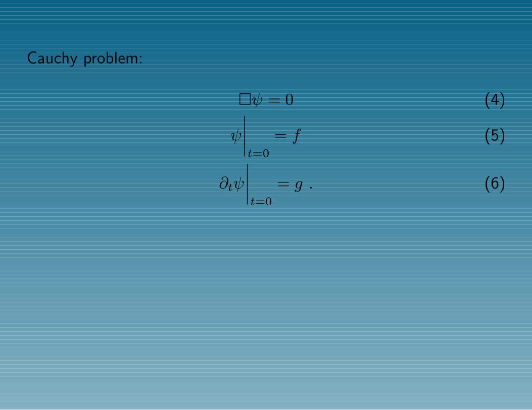
Cauchy problem:
ψ = 0 (4)
ψ
∣∣∣∣t=0
= f (5)
∂tψ
∣∣∣∣t=0
= g . (6)
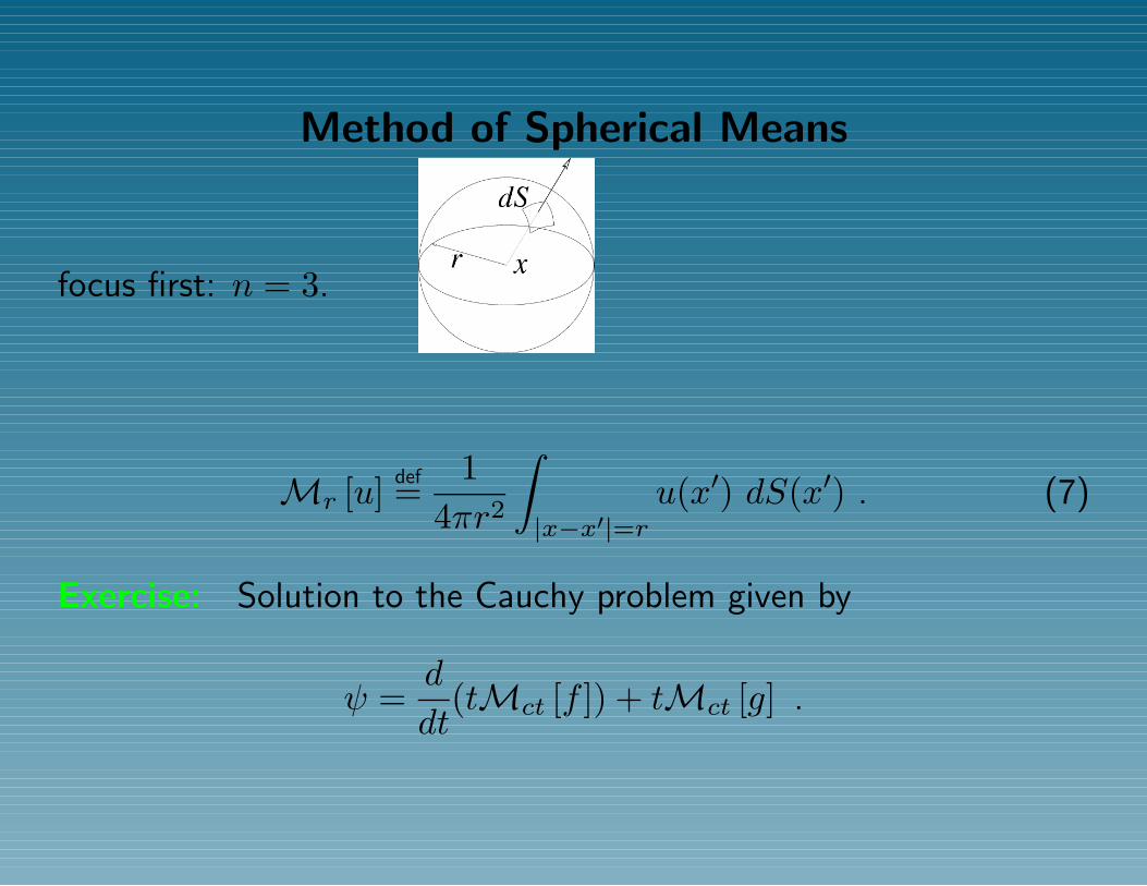
Method of Spherical Means
focus first: n = 3.
Method of Spherical Means
focus first: n = 3.
Mr [u] def=1
4πr2
∫|x−x′|=r
u(x′) dS(x′) . (7)
Exercise: Solution to the Cauchy problem given by
ψ =d
dt(tMct [f ]) + tMct [g] .
Consequence: At the point
(t, x) ∈ R4
solution ψ depends only on the initial data at the points on the
sphere in R3 of radius ct centered at x.
Hadamard’s Method of Descent:
Use the sol. of the given equation in a higher dimensional space to
produce the sol. in a lower dimensional space by introducing extra
“dummy variables.”
Using solutions of the wave eq for n = 3 one obtains a solution of
the wave equation for n = 2.
For n = 2 the dependence is on the interior and the surface of the
ball.
Theorem: For n > 1 odd: Solution of the wave equation depends
on the initial data on the intersection of the light cone with the
initial data manifold t = 0.
For n even: Solution depends on the values of the data on the
closure intersection of the interior part of the light cone and the
initial data manifold t = 0.
Idea of the proof: Use the method of spherical means indicated
above for n odd, and descending to even n.
Remarks on the Strict Huygens Property:
• Fascinating property of the solutions to the wave equation in 3
spatial dimensions
• meaningful transmission of information
• “instantaneous” signal in 3 spatial dimensions remains
“instantaneous”
“Thus our actual physical world, in which acoustic and
electromagnetic signals are the basis of communication, seems
to be singled out among other mathematically conceivable
models by intrinsic simplicity and harmony” (Courant & Hilbert,
Methods of Math. Phys.)
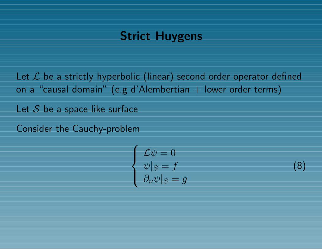
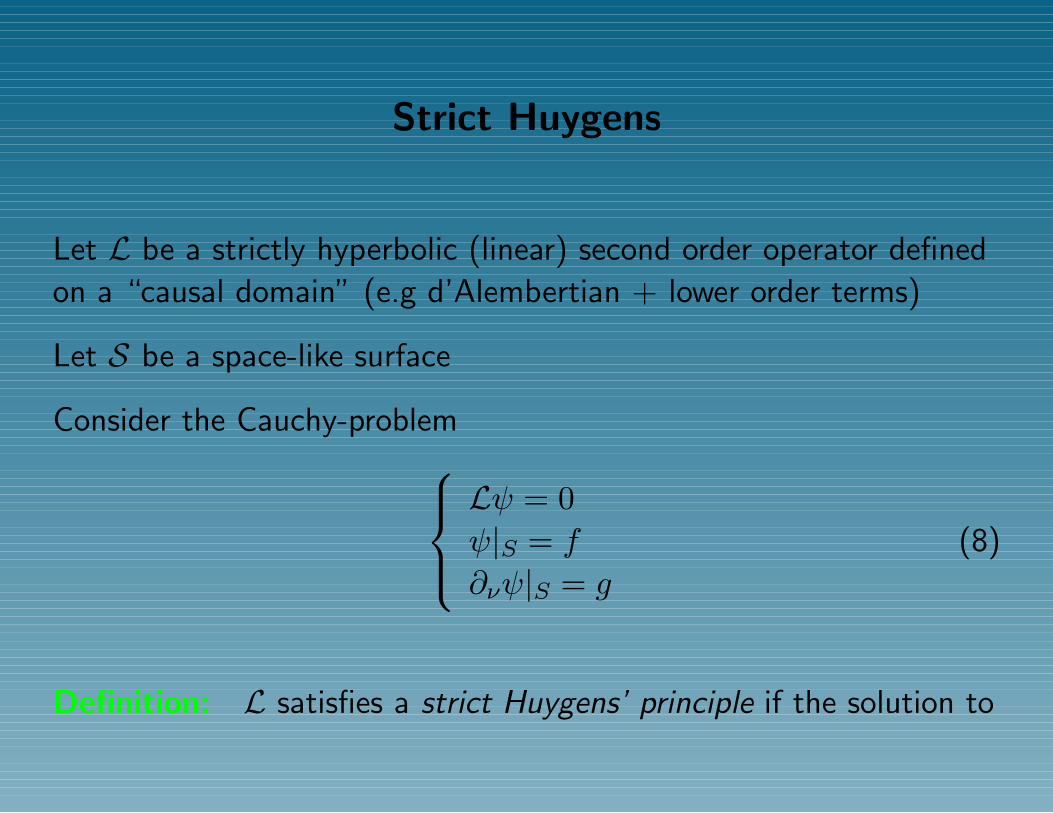
Strict Huygens
Let L be a strictly hyperbolic (linear) second order operator defined
on a “causal domain” (e.g d’Alembertian + lower order terms)
Let S be a space-like surface
Consider the Cauchy-problemLψ = 0ψ|S = f
∂νψ|S = g
(8)
Strict Huygens
Let L be a strictly hyperbolic (linear) second order operator defined
on a “causal domain” (e.g d’Alembertian + lower order terms)
Let S be a space-like surface
Consider the Cauchy-problemLψ = 0ψ|S = f
∂νψ|S = g
(8)
Definition: L satisfies a strict Huygens’ principle if the solution to
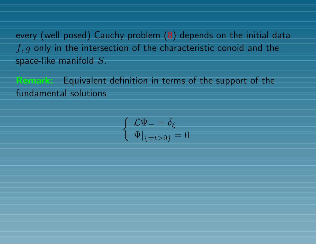
every (well posed) Cauchy problem (8) depends on the initial data
f, g only in the intersection of the characteristic conoid and the
space-like manifold S.
Remark: Equivalent definition in terms of the support of the
fundamental solutions
LΨ± = δξΨ|±t>0 = 0

every (well posed) Cauchy problem (8) depends on the initial data
f, g only in the intersection of the characteristic conoid and the
space-like manifold S.
Remark: Equivalent definition in terms of the support of the
fundamental solutions
LΨ± = δξΨ|±t>0 = 0
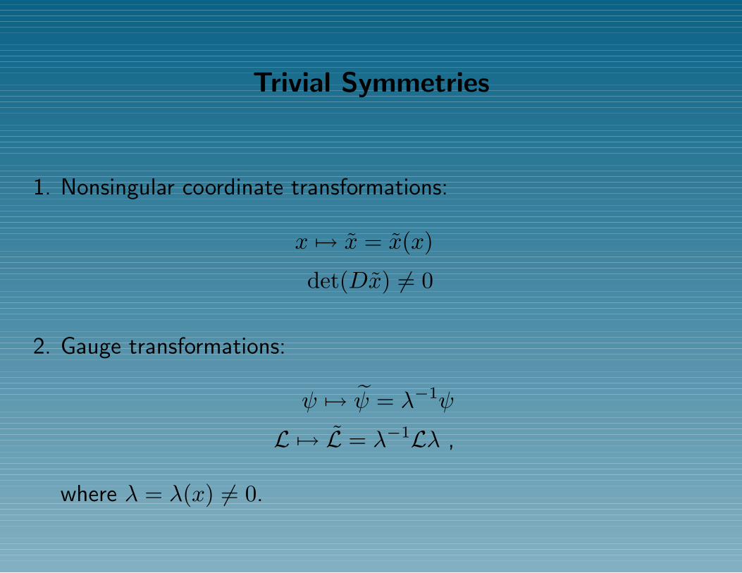
Trivial Symmetries
1. Nonsingular coordinate transformations:
x 7→ x = x(x)
det(Dx) 6= 0
2. Gauge transformations:
ψ 7→ ψ = λ−1ψ
L 7→ L = λ−1Lλ ,
where λ = λ(x) 6= 0.
3. Multiplication by a scalar function:
L 7→ L = µL ,
where µ = µ(x) 6= 0.
Hadamard’s Question:
Determine all the hyperbolic operators that satisfy a strict Huygens’
Property (HP).
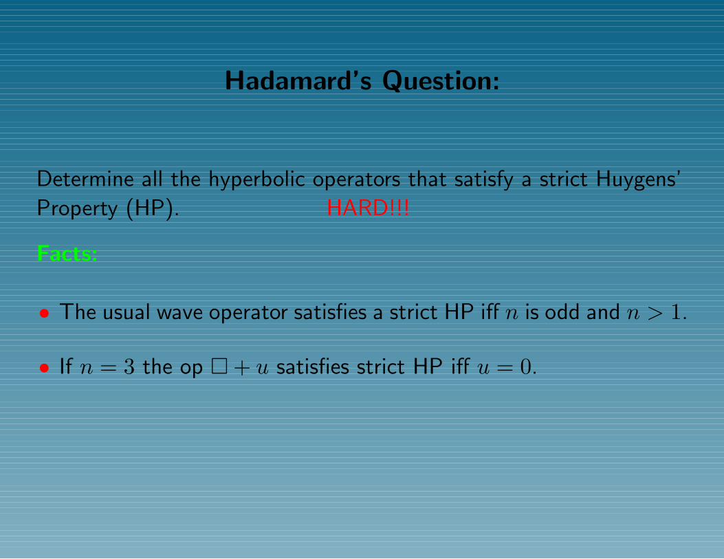
Hadamard’s Question:
Determine all the hyperbolic operators that satisfy a strict Huygens’
Property (HP). HARD!!!
Facts:
• The usual wave operator satisfies a strict HP iff n is odd and n > 1.
• If n = 3 the op + u satisfies strict HP iff u = 0.
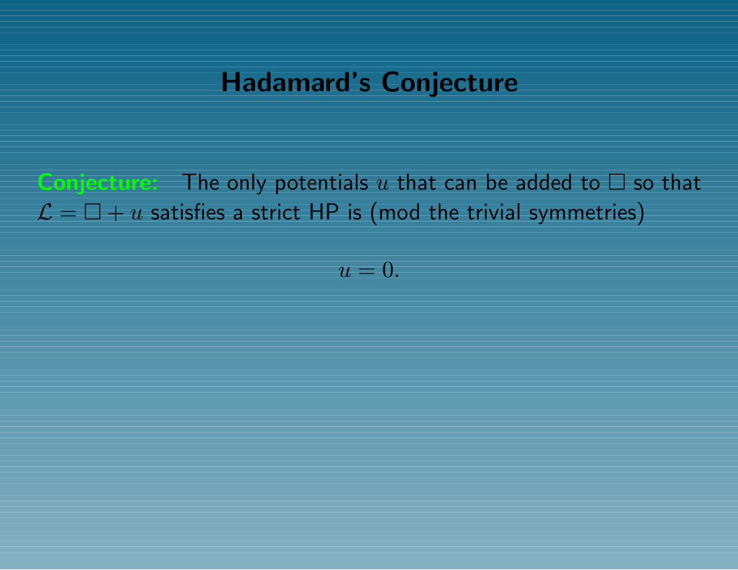
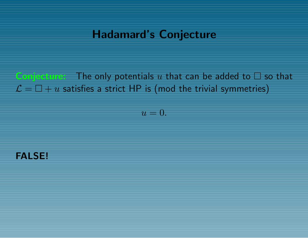
Hadamard’s Conjecture
Conjecture: The only potentials u that can be added to so that
L = + u satisfies a strict HP is (mod the trivial symmetries)
u = 0.
Hadamard’s Conjecture
Conjecture: The only potentials u that can be added to so that
L = + u satisfies a strict HP is (mod the trivial symmetries)
u = 0.
FALSE!
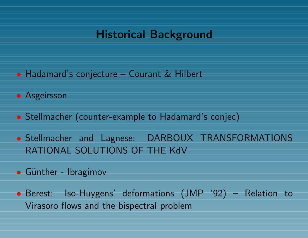
Historical Background
• Hadamard’s conjecture – Courant & Hilbert
• Asgeirsson
• Stellmacher (counter-example to Hadamard’s conjec)
• Stellmacher and Lagnese: DARBOUX TRANSFORMATIONS
RATIONAL SOLUTIONS OF THE KdV
• Gunther - Ibragimov
• Berest: Iso-Huygens’ deformations (JMP ‘92) – Relation to
Virasoro flows and the bispectral problem
“The symmetries that preserve HP for operators of the form
+ u(x0) are related to the symmetries that preserve the bispectral
property for u(x0), i.e., the positive Virasoro flows”
“The symmetries that preserve HP for operators of the form
+ u(x0) are related to the symmetries that preserve the bispectral
property for u(x0), i.e., the positive Virasoro flows” related to joint
work w/ F. Magri. CMP 1992
Lagnese & Stellmacher
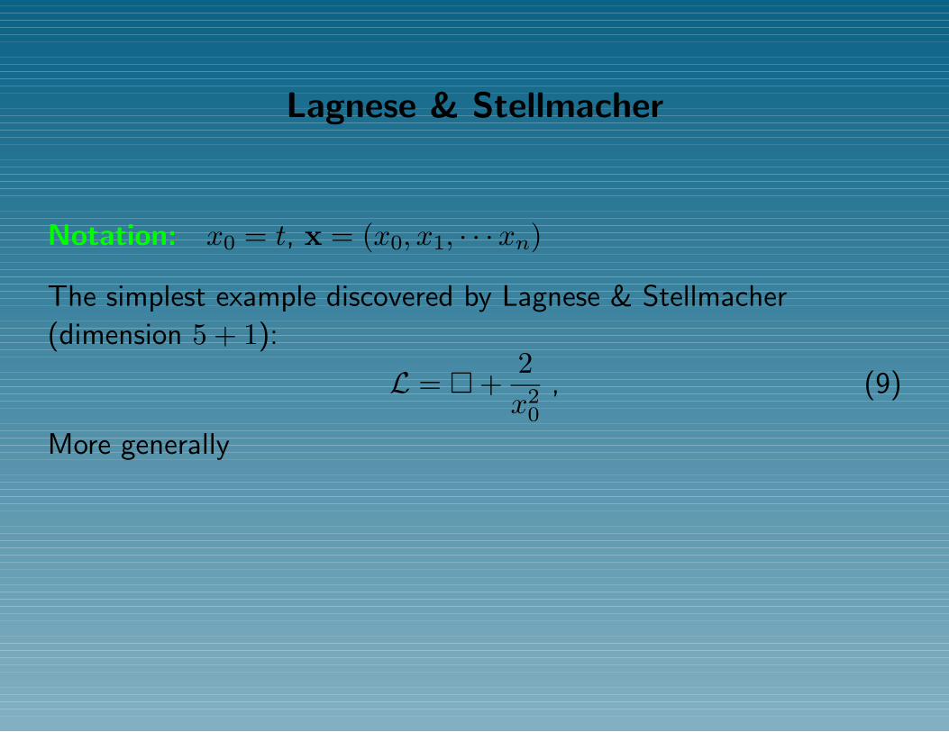
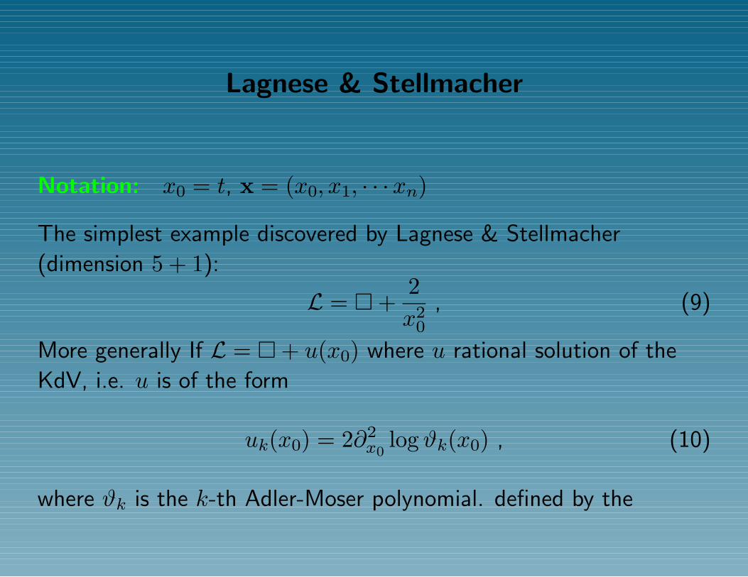
Notation: x0 = t, x = (x0, x1, · · ·xn)
The simplest example discovered by Lagnese & Stellmacher
(dimension 5 + 1):
L = +2x2
0
, (9)
More generally
Lagnese & Stellmacher
Notation: x0 = t, x = (x0, x1, · · ·xn)
The simplest example discovered by Lagnese & Stellmacher
(dimension 5 + 1):
L = +2x2
0
, (9)
More generally If L = + u(x0) where u rational solution of the
KdV, i.e. u is of the form
uk(x0) = 2∂2x0
log ϑk(x0) , (10)
where ϑk is the k-th Adler-Moser polynomial. defined by the
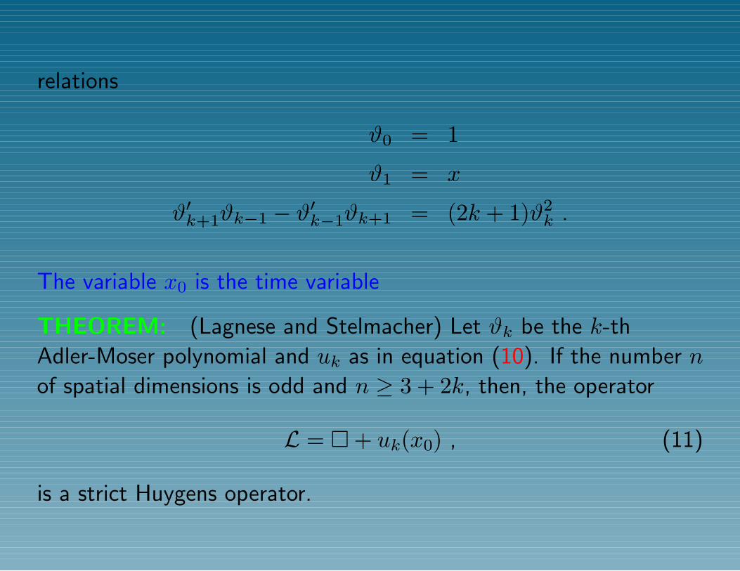
relations
ϑ0 = 1
ϑ1 = x
ϑ′k+1ϑk−1 − ϑ′k−1ϑk+1 = (2k + 1)ϑ2k .
The variable x0 is the time variable
THEOREM: (Lagnese and Stelmacher) Let ϑk be the k-th
Adler-Moser polynomial and uk as in equation (10). If the number n
of spatial dimensions is odd and n ≥ 3 + 2k, then, the operator
L = + uk(x0) , (11)
is a strict Huygens operator.
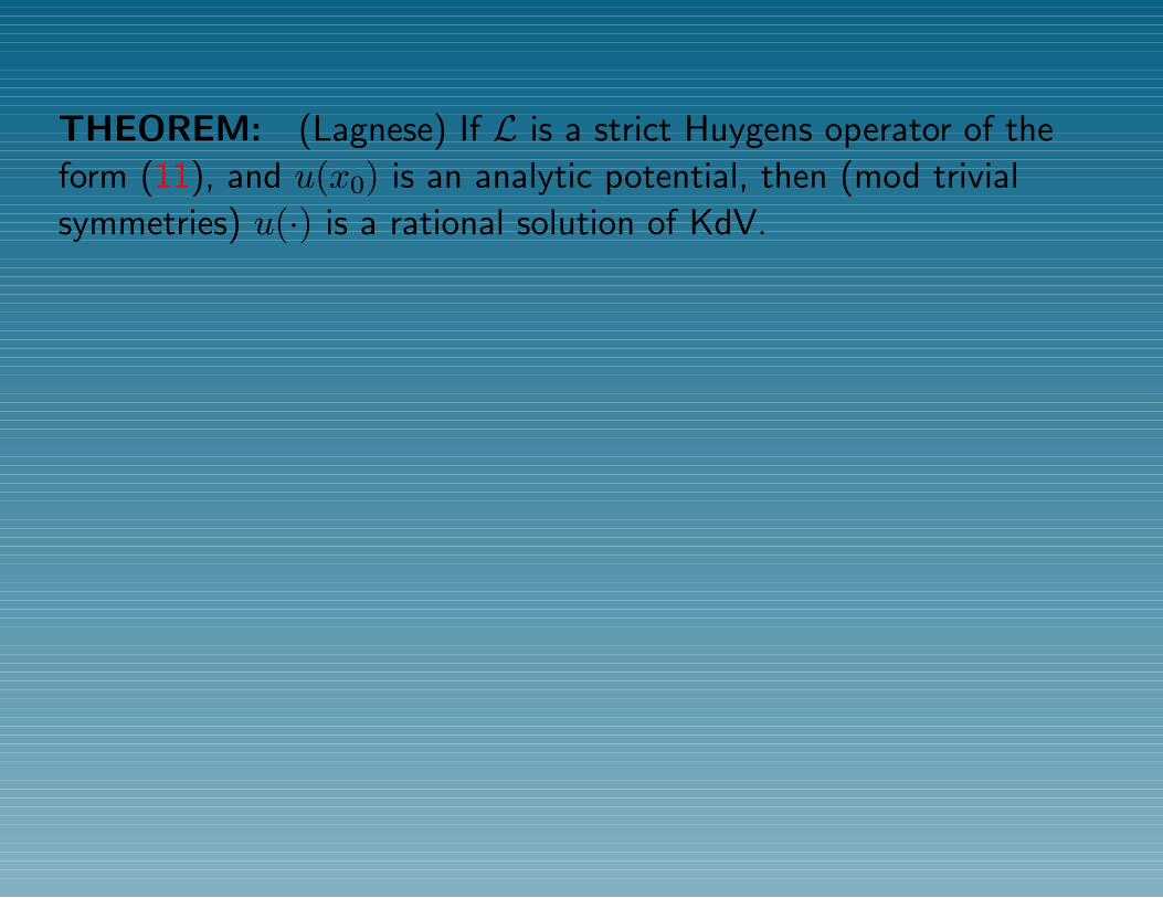
THEOREM: (Lagnese) If L is a strict Huygens operator of the
form (11), and u(x0) is an analytic potential, then (mod trivial
symmetries) u(·) is a rational solution of KdV.
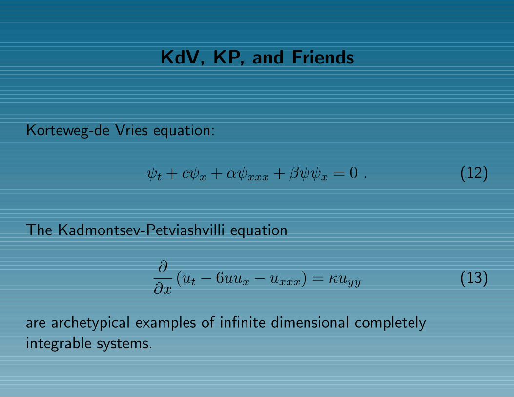
KdV, KP, and Friends
Korteweg-de Vries equation:
ψt + cψx + αψxxx + βψψx = 0 . (12)
The Kadmontsev-Petviashvilli equation
∂
∂x(ut − 6uux − uxxx) = κuyy (13)
are archetypical examples of infinite dimensional completely
integrable systems.
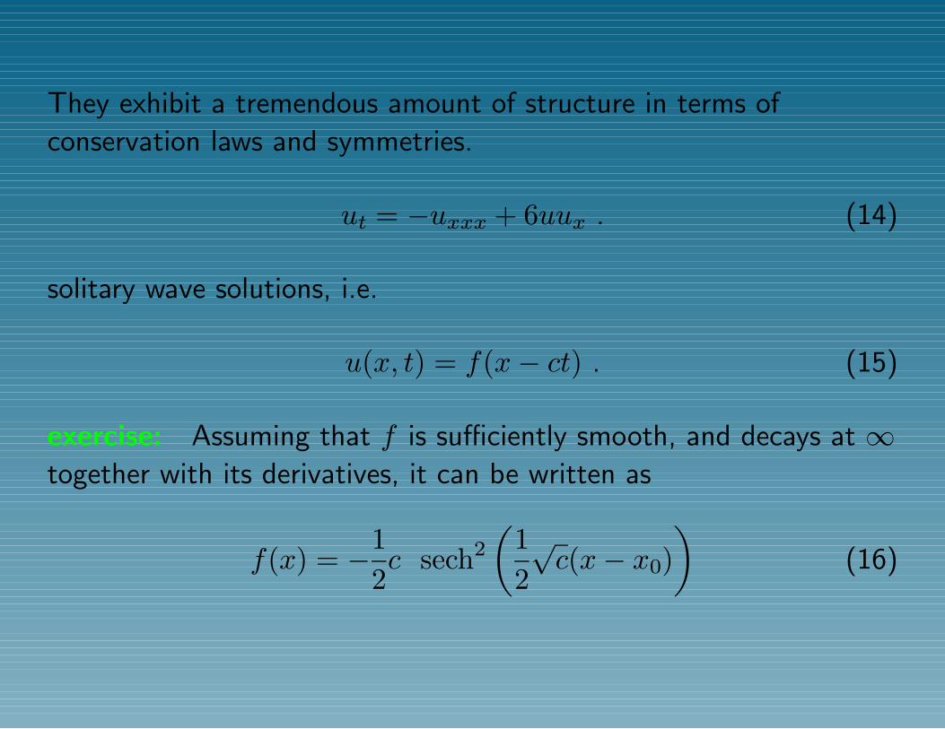
They exhibit a tremendous amount of structure in terms of
conservation laws and symmetries.
ut = −uxxx + 6uux . (14)
solitary wave solutions, i.e.
u(x, t) = f(x− ct) . (15)
exercise: Assuming that f is sufficiently smooth, and decays at ∞together with its derivatives, it can be written as
f(x) = −12c sech2
(12√c(x− x0)
)(16)

The J. S. Russel Story
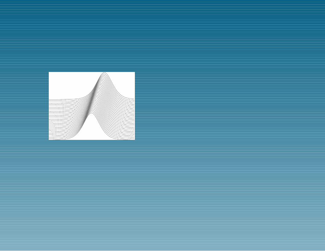
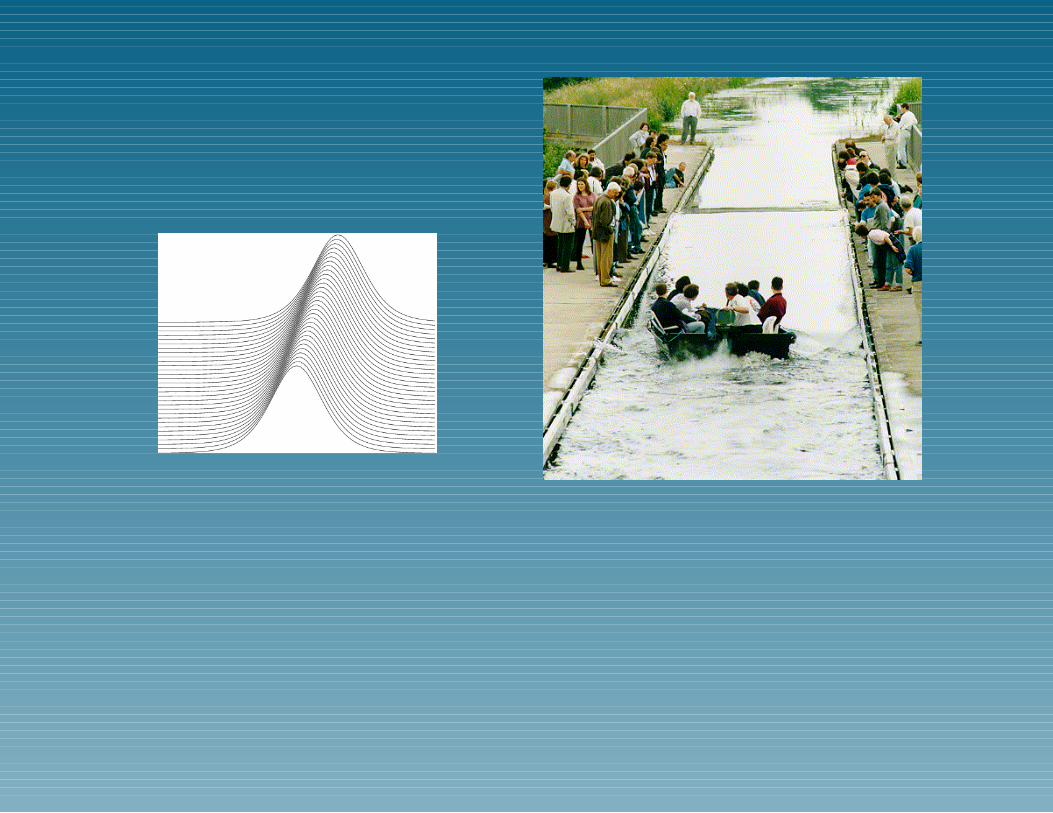
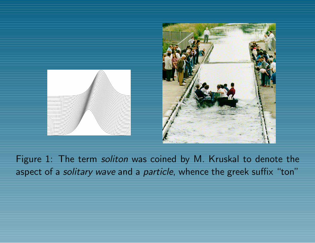
Figure 1: The term soliton was coined by M. Kruskal to denote the
aspect of a solitary wave and a particle, whence the greek suffix “ton”
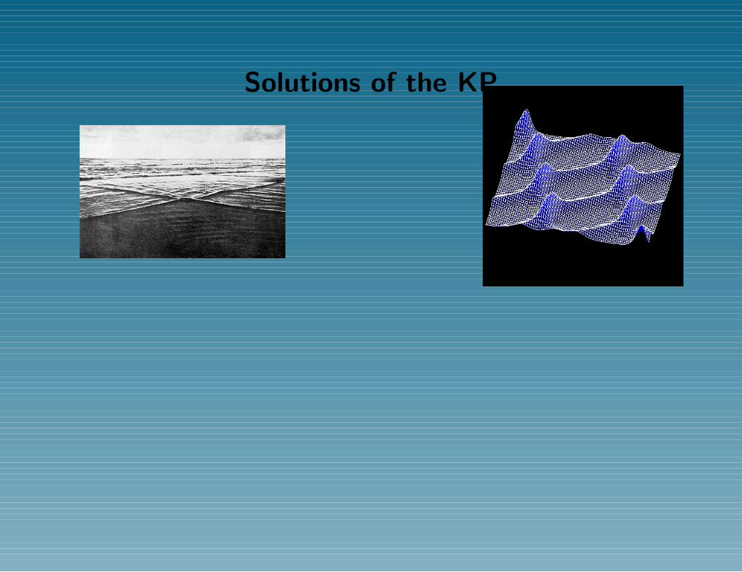
Solutions of the KP
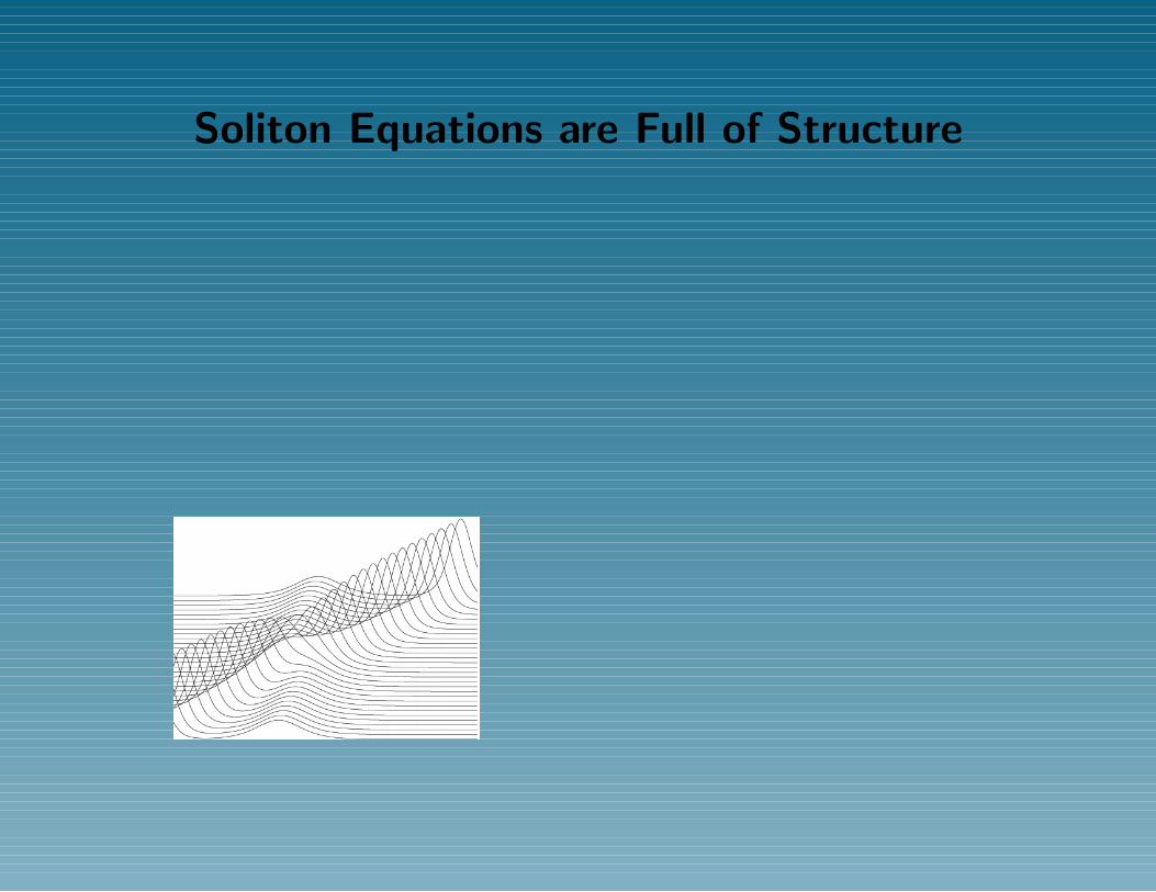
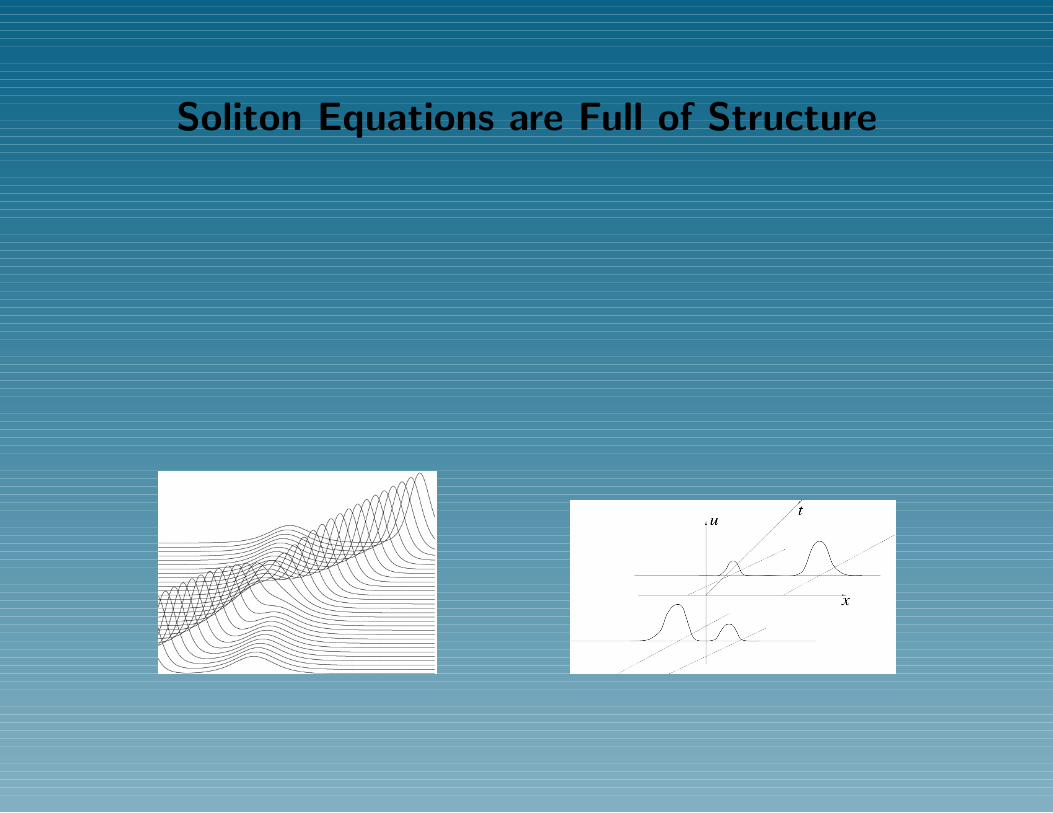
Soliton Equations are Full of Structure

Soliton Equations are Full of Structure
Soliton Equations are Full of Structure
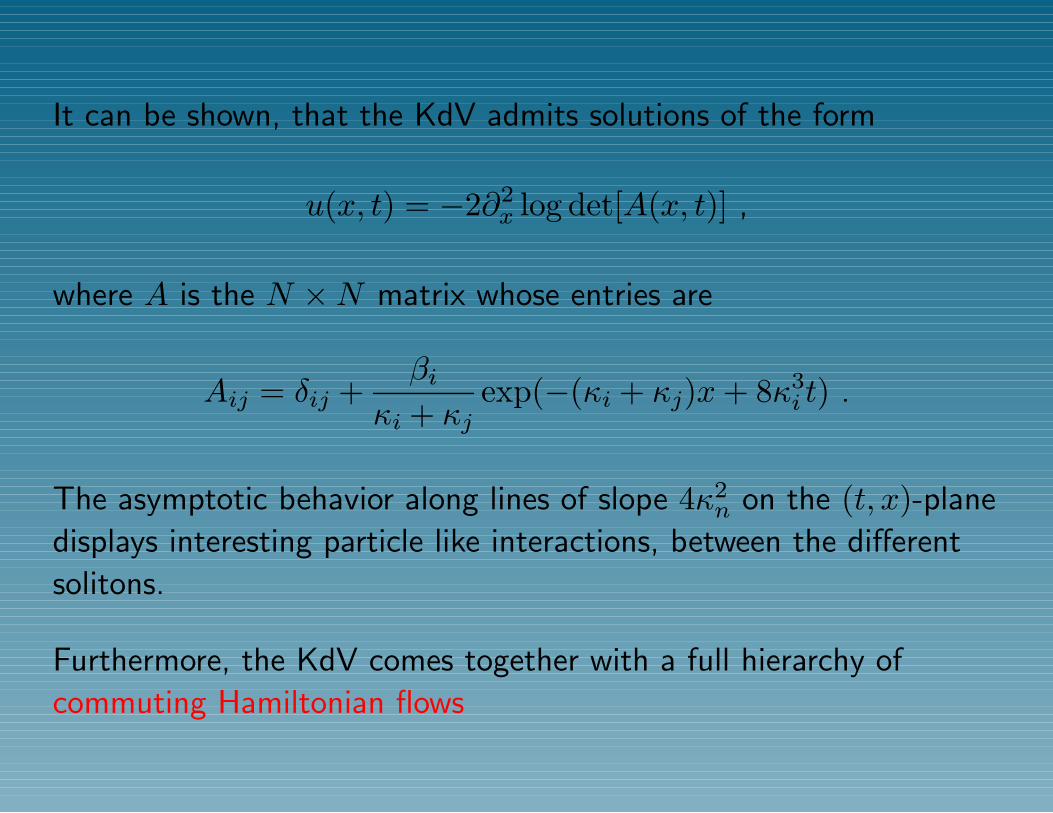
It can be shown, that the KdV admits solutions of the form
u(x, t) = −2∂2x log det[A(x, t)] ,
where A is the N ×N matrix whose entries are
Aij = δij +βi
κi + κjexp(−(κi + κj)x+ 8κ3
i t) .
The asymptotic behavior along lines of slope 4κ2n on the (t, x)-plane
displays interesting particle like interactions, between the different
solitons.
Furthermore, the KdV comes together with a full hierarchy of
commuting Hamiltonian flows
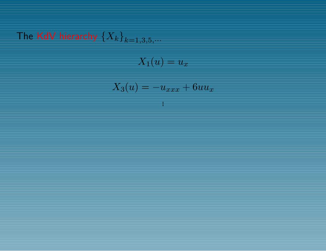
The KdV hierarchy Xkk=1,3,5,···
X1(u) = ux
X3(u) = −uxxx + 6uux...
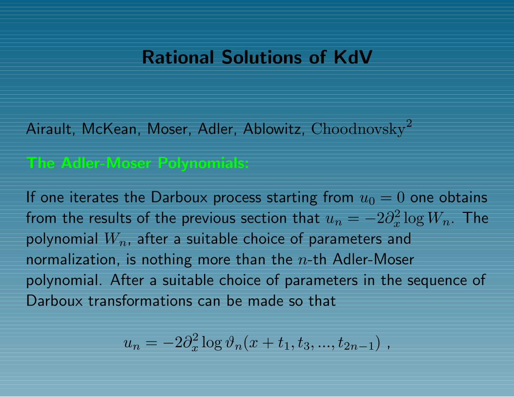
Rational Solutions of KdV
Airault, McKean, Moser, Adler, Ablowitz, Choodnovsky2
The Adler-Moser Polynomials:
If one iterates the Darboux process starting from u0 = 0 one obtains
from the results of the previous section that un = −2∂2x logWn. The
polynomial Wn, after a suitable choice of parameters and
normalization, is nothing more than the n-th Adler-Moser
polynomial. After a suitable choice of parameters in the sequence of
Darboux transformations can be made so that
un = −2∂2x log ϑn(x+ t1, t3, ..., t2n−1) ,
satisfies the flows of the KdV hierarchy, i.e.,
∂tkun = Xk[un] .
Furthermore:
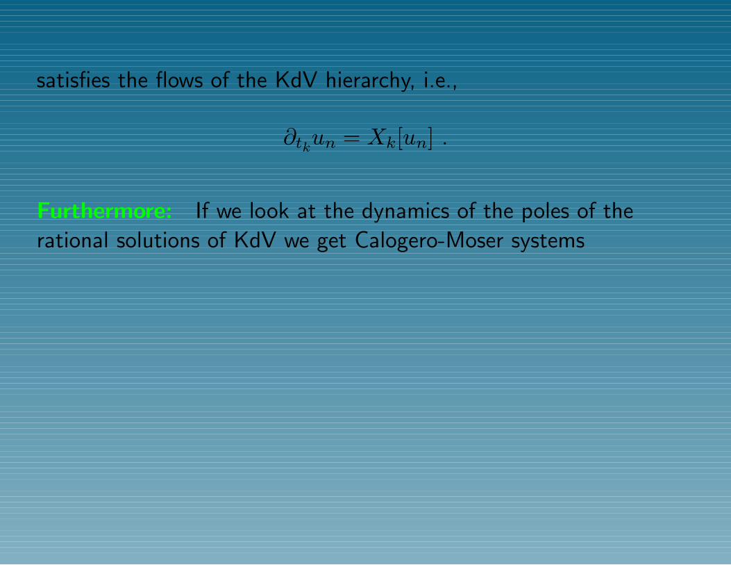
satisfies the flows of the KdV hierarchy, i.e.,
∂tkun = Xk[un] .
Furthermore: If we look at the dynamics of the poles of the
rational solutions of KdV we get Calogero-Moser systems
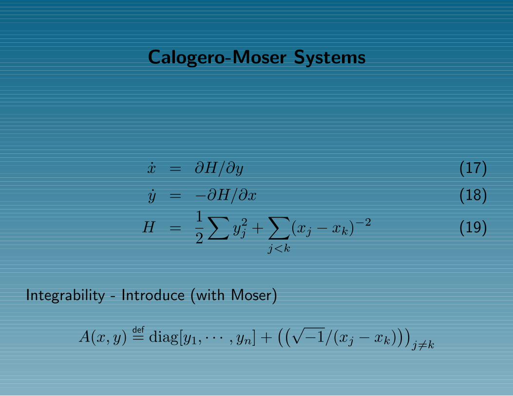
Calogero-Moser Systems
x = ∂H/∂y (17)
y = −∂H/∂x (18)
H =12
∑y2j +
∑j<k
(xj − xk)−2 (19)
Integrability - Introduce (with Moser)
A(x, y) def= diag[y1, · · · , yn] +((√−1/(xj − xk)
))j 6=k
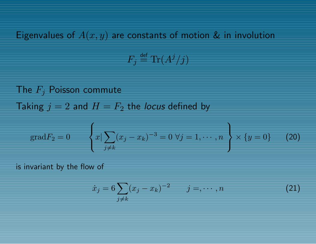
Eigenvalues of A(x, y) are constants of motion & in involution
Fjdef= Tr(Aj/j)
The Fj Poisson commute
Taking j = 2 and H = F2 the locus defined by
gradF2 = 0
x|∑j 6=k
(xj − xk)−3 = 0 ∀j = 1, · · · , n
× y = 0 (20)
is invariant by the flow of
xj = 6∑j 6=k
(xj − xk)−2 j =, · · · , n (21)
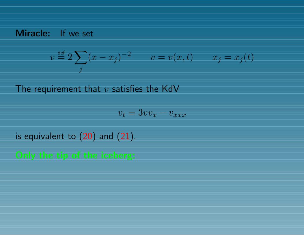
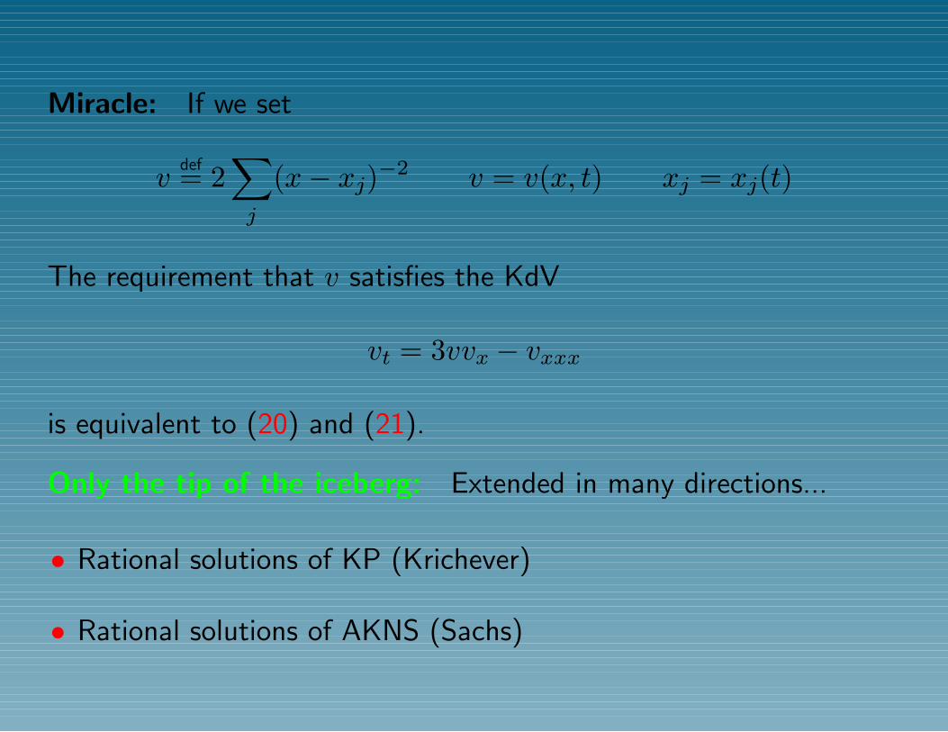
Miracle: If we set
vdef= 2
∑j
(x− xj)−2 v = v(x, t) xj = xj(t)
The requirement that v satisfies the KdV
vt = 3vvx − vxxx
is equivalent to (20) and (21).
Only the tip of the iceberg:
Miracle: If we set
vdef= 2
∑j
(x− xj)−2 v = v(x, t) xj = xj(t)
The requirement that v satisfies the KdV
vt = 3vvx − vxxx
is equivalent to (20) and (21).
Only the tip of the iceberg: Extended in many directions...
• Rational solutions of KP (Krichever)
• Rational solutions of AKNS (Sachs)

AKNS: Ablowitz-Kaup-Newell-Segur-Zakharov-Shabat Obtained a
way of constructing certain hierarchies of integrable evolution
equations.
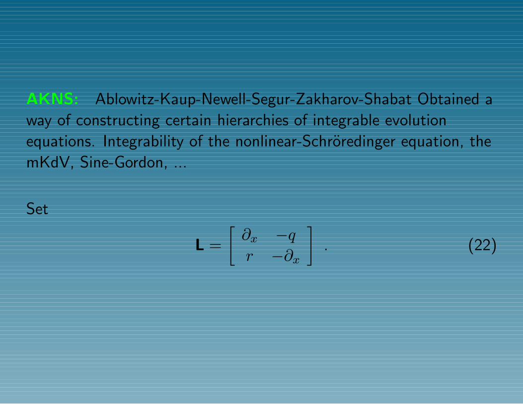
AKNS: Ablowitz-Kaup-Newell-Segur-Zakharov-Shabat Obtained a
way of constructing certain hierarchies of integrable evolution
equations. Integrability of the nonlinear-Schroredinger equation, the
mKdV, Sine-Gordon, ...
Set
L =[∂x −qr −∂x
]. (22)
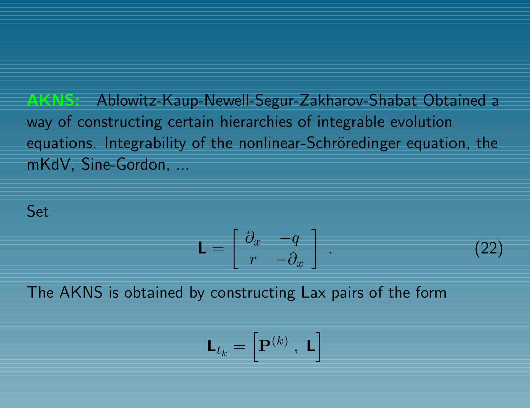
AKNS: Ablowitz-Kaup-Newell-Segur-Zakharov-Shabat Obtained a
way of constructing certain hierarchies of integrable evolution
equations. Integrability of the nonlinear-Schroredinger equation, the
mKdV, Sine-Gordon, ...
Set
L =[∂x −qr −∂x
]. (22)
The AKNS is obtained by constructing Lax pairs of the form
Ltk =[P(k) , L
]
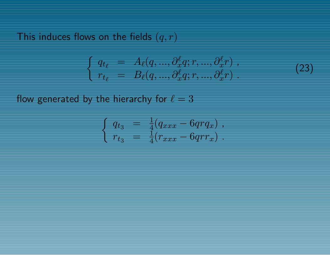
This induces flows on the fields (q, r)qt` = A`(q, ..., ∂`xq; r, ..., ∂
`xr) ,
rt` = B`(q, ..., ∂`xq; r, ..., ∂`xr) .
(23)
flow generated by the hierarchy for ` = 3qt3 = 1
4(qxxx − 6qrqx) ,
rt3 = 14(rxxx − 6qrrx) .
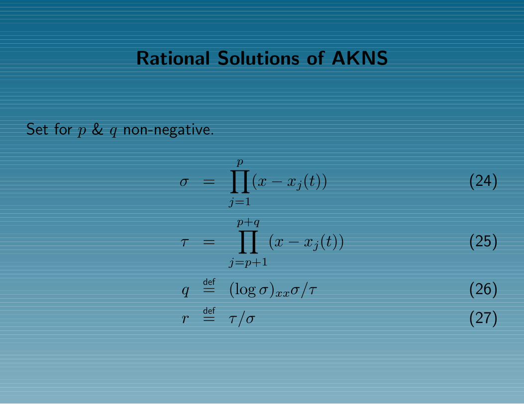
Rational Solutions of AKNS
Set for p & q non-negative.
σ =p∏j=1
(x− xj(t)) (24)
τ =p+q∏j=p+1
(x− xj(t)) (25)
qdef= (log σ)xxσ/τ (26)
rdef= τ/σ (27)
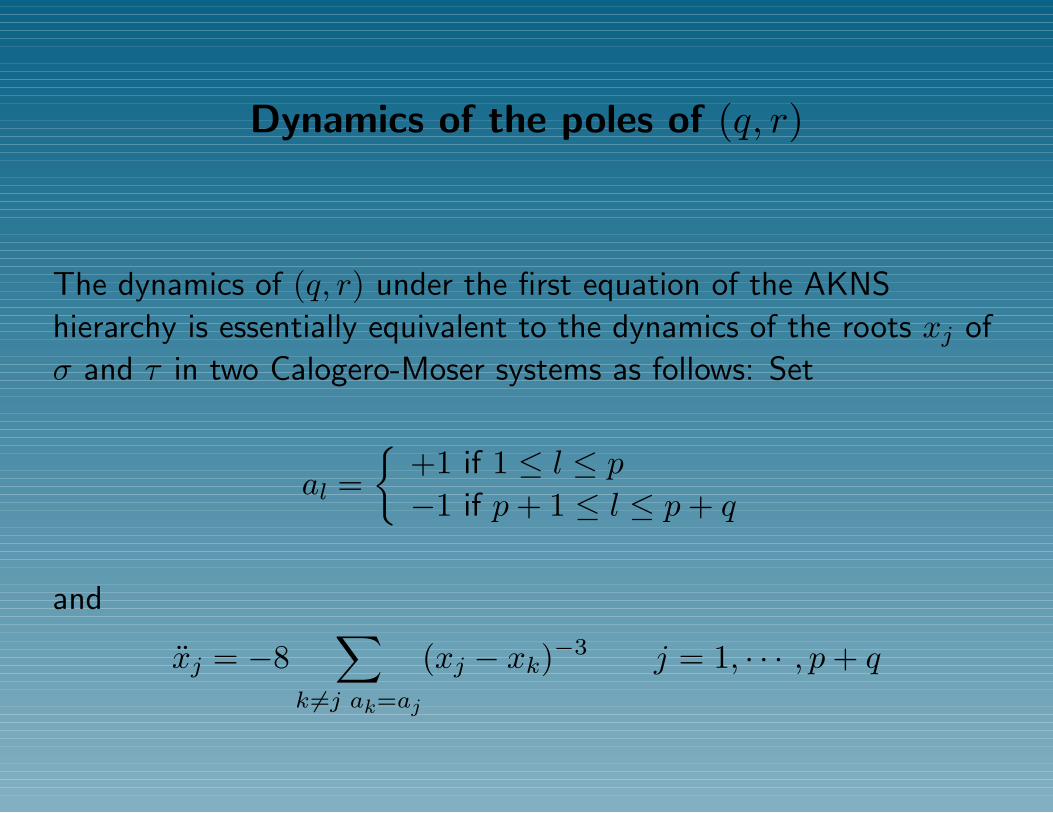
Dynamics of the poles of (q, r)
The dynamics of (q, r) under the first equation of the AKNS
hierarchy is essentially equivalent to the dynamics of the roots xj of
σ and τ in two Calogero-Moser systems as follows: Set
al =
+1 if 1 ≤ l ≤ p−1 if p+ 1 ≤ l ≤ p+ q
and
xj = −8∑
k 6=j ak=aj
(xj − xk)−3 j = 1, · · · , p+ q
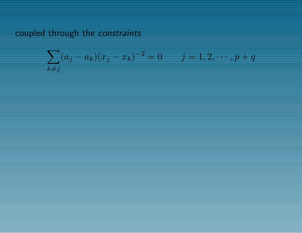
coupled through the constraints∑k 6=j
(aj − ak)(xj − xk)−2 = 0 j = 1, 2, · · · , p+ q
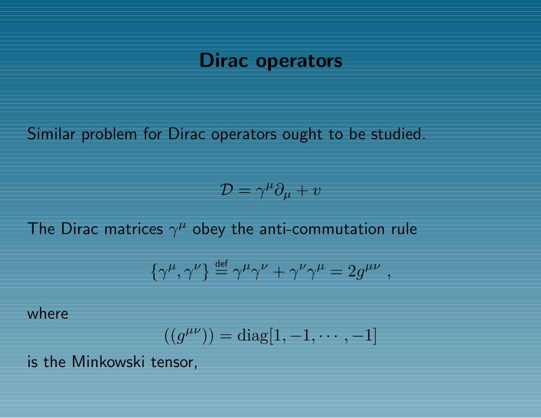
Dirac operators
Similar problem for Dirac operators ought to be studied.
D = γµ∂µ + v
The Dirac matrices γµ obey the anti-commutation rule
γµ, γν def= γµγν + γνγµ = 2gµν ,
where
((gµν)) = diag[1,−1, · · · ,−1]
is the Minkowski tensor,
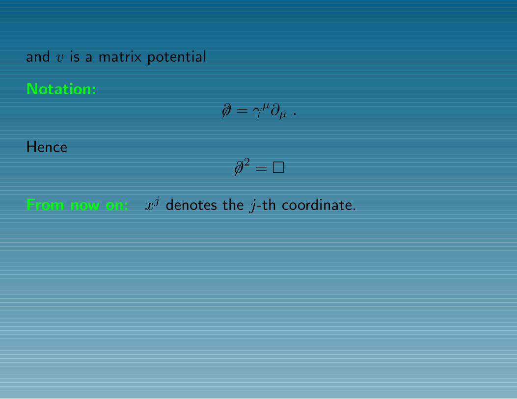
and v is a matrix potential
Notation:6∂ = γµ∂µ .
Hence
6∂2 =
From now on: xj denotes the j-th coordinate.
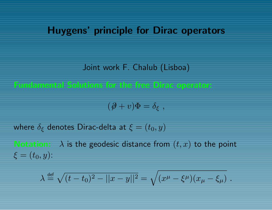
Huygens’ principle for Dirac operators
Joint work F. Chalub (Lisboa)
Fundamental Solutions for the free Dirac operator:
(6∂ + v)Φ = δξ ,
where δξ denotes Dirac-delta at ξ = (t0, y)
Notation: λ is the geodesic distance from (t, x) to the point
ξ = (t0, y):
λdef=√
(t− t0)2 − ||x− y||2 =√
(xµ − ξµ)(xµ − ξµ) .
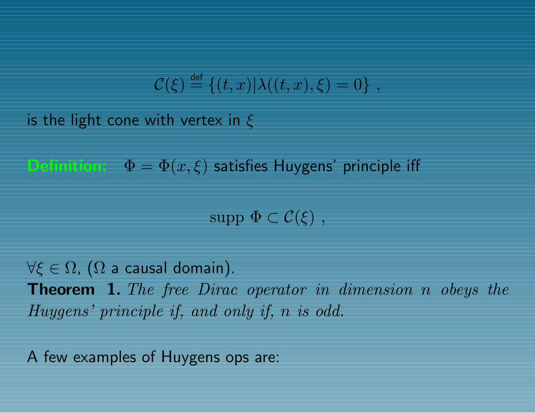
C(ξ) def= (t, x)|λ((t, x), ξ) = 0 ,
is the light cone with vertex in ξ
Definition: Φ = Φ(x, ξ) satisfies Huygens’ principle iff
supp Φ ⊂ C(ξ) ,
∀ξ ∈ Ω, (Ω a causal domain).
Theorem 1. The free Dirac operator in dimension n obeys theHuygens’ principle if, and only if, n is odd.
A few examples of Huygens ops are:
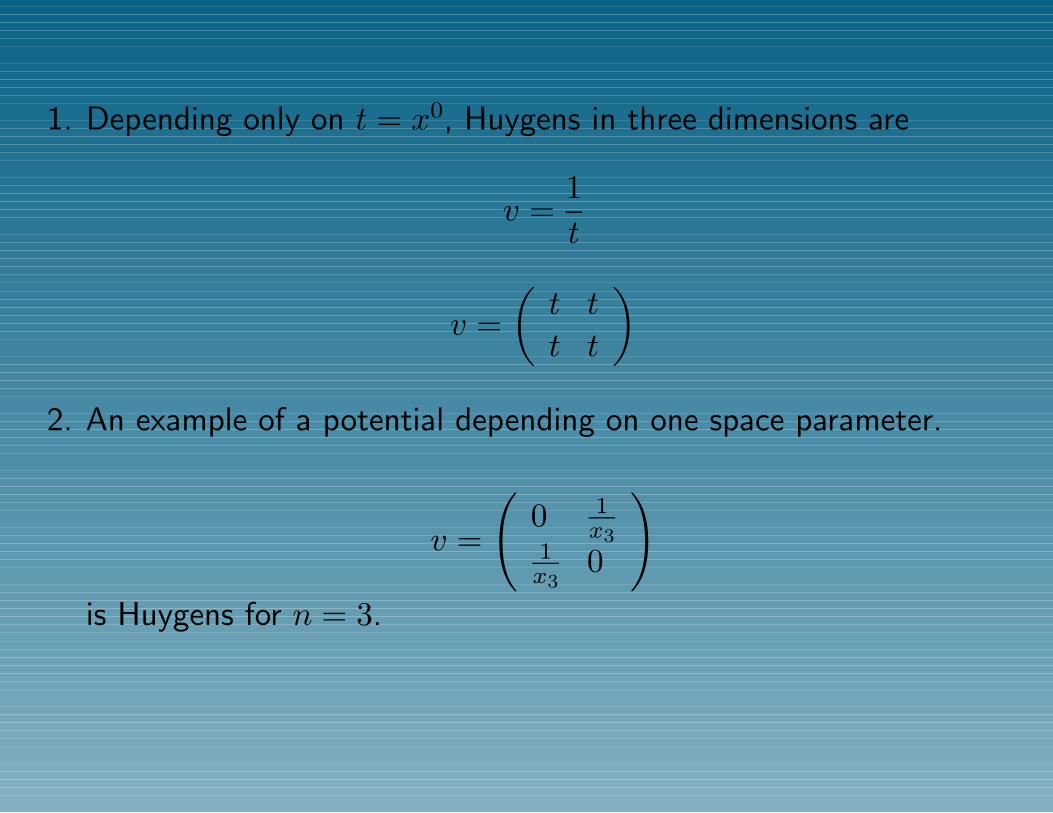
1. Depending only on t = x0, Huygens in three dimensions are
v =1t
v =(t t
t t
)2. An example of a potential depending on one space parameter.
v =
(0 1
x31x3
0
)is Huygens for n = 3.
Natural Question: Can one construct a family of (strict) Huygens
Dirac operators similar to the one obtained by Lagnese and
Stellmacher for the wave operator?
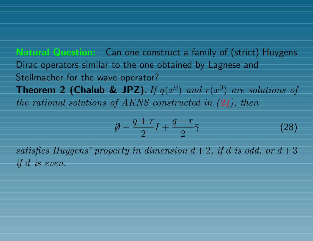
Natural Question: Can one construct a family of (strict) Huygens
Dirac operators similar to the one obtained by Lagnese and
Stellmacher for the wave operator?
Theorem 2 (Chalub & JPZ). If q(x0) and r(x0) are solutions ofthe rational solutions of AKNS constructed in (24), then
6∂ − q + r
2I +
q − r2
γ (28)
satisfies Huygens’ property in dimension d+2, if d is odd, or d+3if d is even.
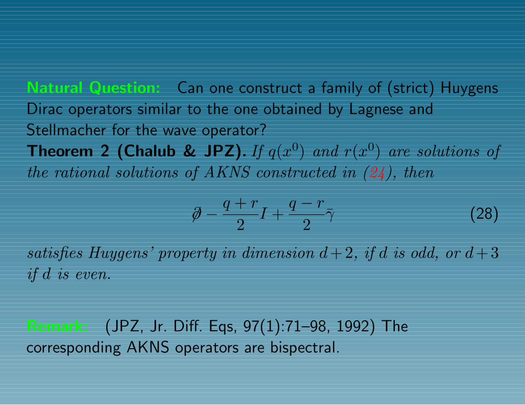
Remark: (JPZ, Jr. Diff. Eqs, 97(1):71–98, 1992) The
corresponding AKNS operators are bispectral.
Technical Details
Construction of Fundamental Solutions:
LF = δ
Technical Details
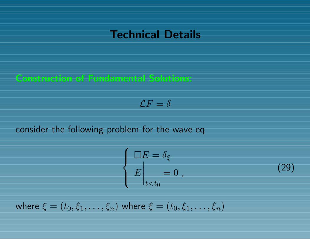
Construction of Fundamental Solutions:
LF = δ
consider the following problem for the wave eqE = δξ
E
∣∣∣∣t<t0
= 0 ,(29)
where ξ = (t0, ξ1, . . . , ξn) where ξ = (t0, ξ1, . . . , ξn)
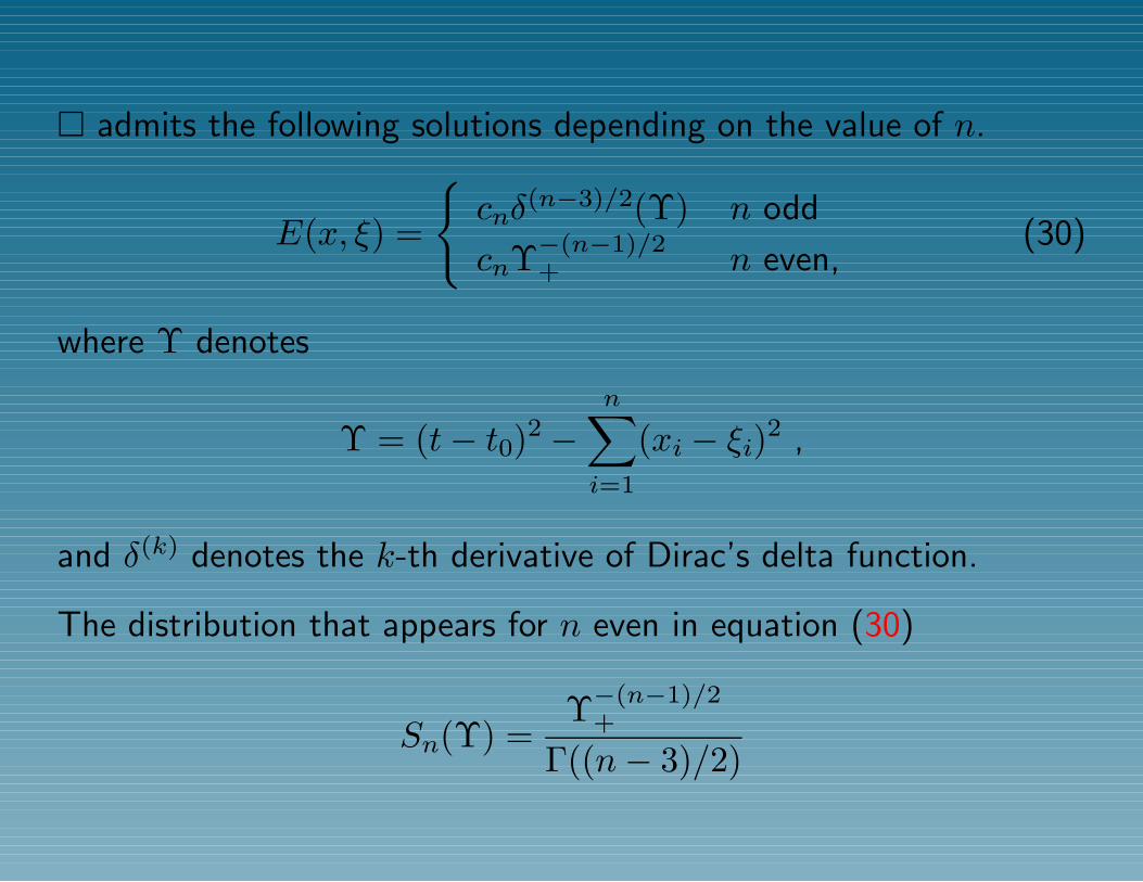
admits the following solutions depending on the value of n.
E(x, ξ) =
cnδ
(n−3)/2(Υ) n odd
cnΥ−(n−1)/2+ n even,
(30)
where Υ denotes
Υ = (t− t0)2 −n∑i=1
(xi − ξi)2 ,
and δ(k) denotes the k-th derivative of Dirac’s delta function.
The distribution that appears for n even in equation (30)
Sn(Υ) =Υ−(n−1)/2
+
Γ((n− 3)/2)
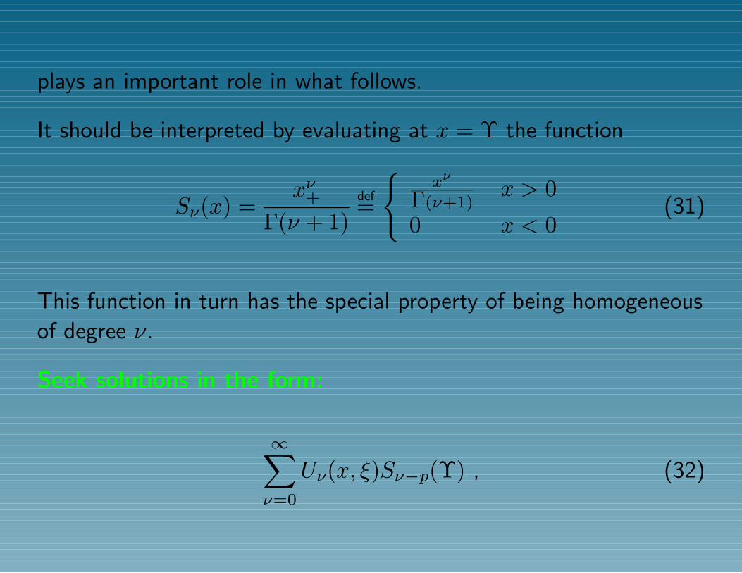
plays an important role in what follows.
It should be interpreted by evaluating at x = Υ the function
Sν(x) =xν+
Γ(ν + 1)def=
xν
Γ(ν+1)x > 0
0 x < 0(31)
This function in turn has the special property of being homogeneous
of degree ν.
Seek solutions in the form:
∞∑ν=0
Uν(x, ξ)Sν−p(Υ) , (32)
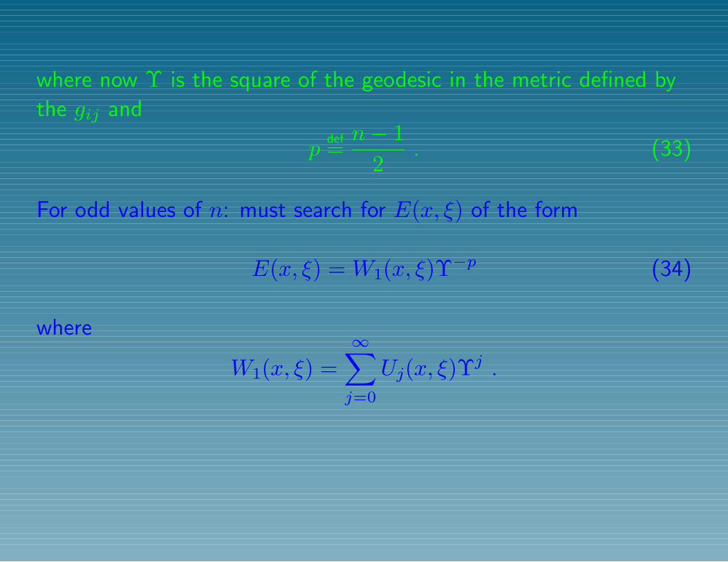
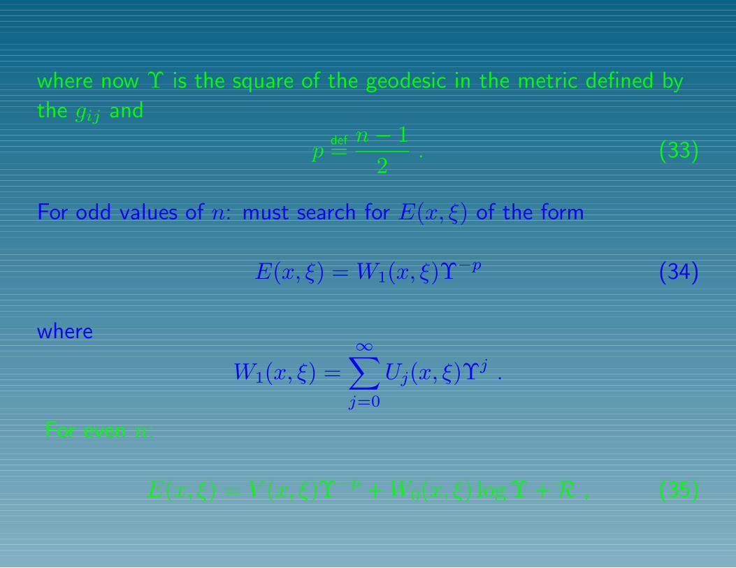
where now Υ is the square of the geodesic in the metric defined by
the gij and
pdef=n− 1
2. (33)
For odd values of n: must search for E(x, ξ) of the form
E(x, ξ) = W1(x, ξ)Υ−p (34)
where
W1(x, ξ) =∞∑j=0
Uj(x, ξ)Υj .
where now Υ is the square of the geodesic in the metric defined by
the gij and
pdef=n− 1
2. (33)
For odd values of n: must search for E(x, ξ) of the form
E(x, ξ) = W1(x, ξ)Υ−p (34)
where
W1(x, ξ) =∞∑j=0
Uj(x, ξ)Υj .
For even n:
E(x, ξ) = V (x, ξ)Υ−p +W0(x, ξ) log Υ +R , (35)
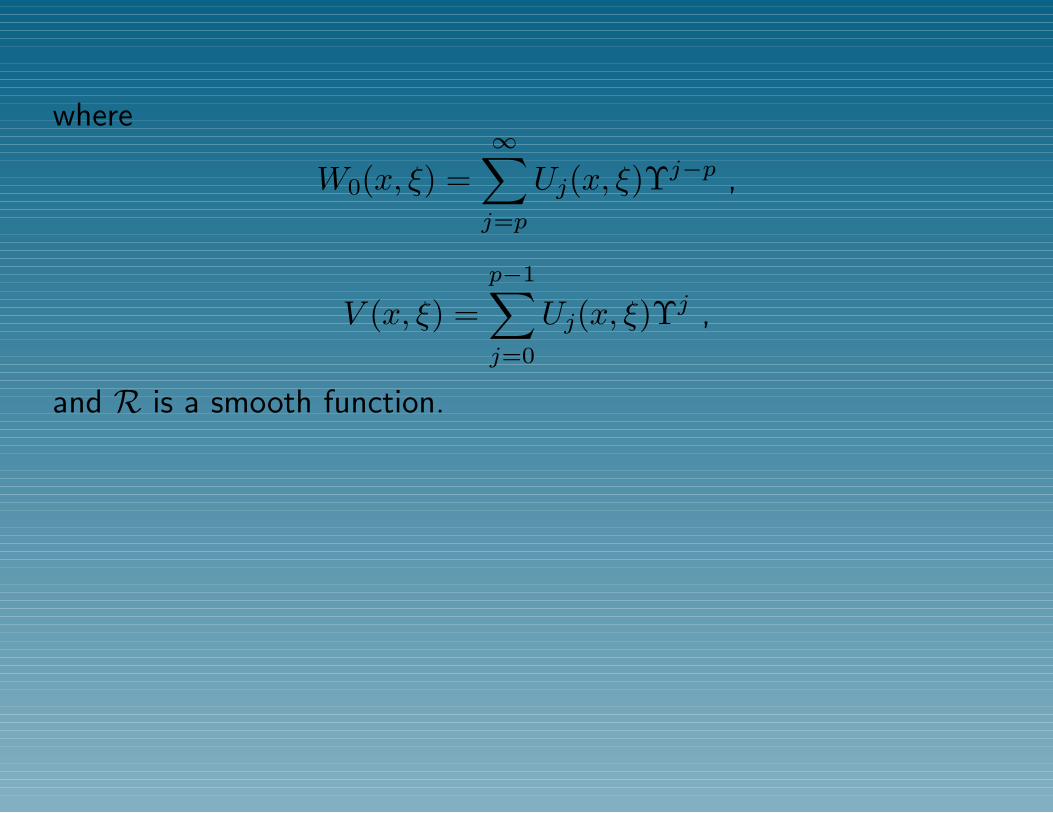
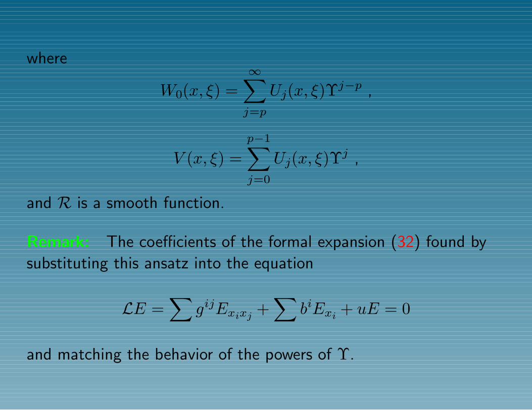
where
W0(x, ξ) =∞∑j=p
Uj(x, ξ)Υj−p ,
V (x, ξ) =p−1∑j=0
Uj(x, ξ)Υj ,
and R is a smooth function.
where
W0(x, ξ) =∞∑j=p
Uj(x, ξ)Υj−p ,
V (x, ξ) =p−1∑j=0
Uj(x, ξ)Υj ,
and R is a smooth function.
Remark: The coefficients of the formal expansion (32) found by
substituting this ansatz into the equation
LE =∑
gijExixj +∑
biExi + uE = 0
and matching the behavior of the powers of Υ.
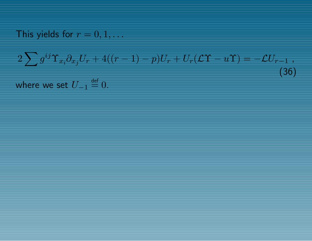
This yields for r = 0, 1, . . .
2∑
gijΥxi∂xjUr + 4((r − 1)− p)Ur + Ur(LΥ− uΥ) = −LUr−1 ,
(36)
where we set U−1def= 0.
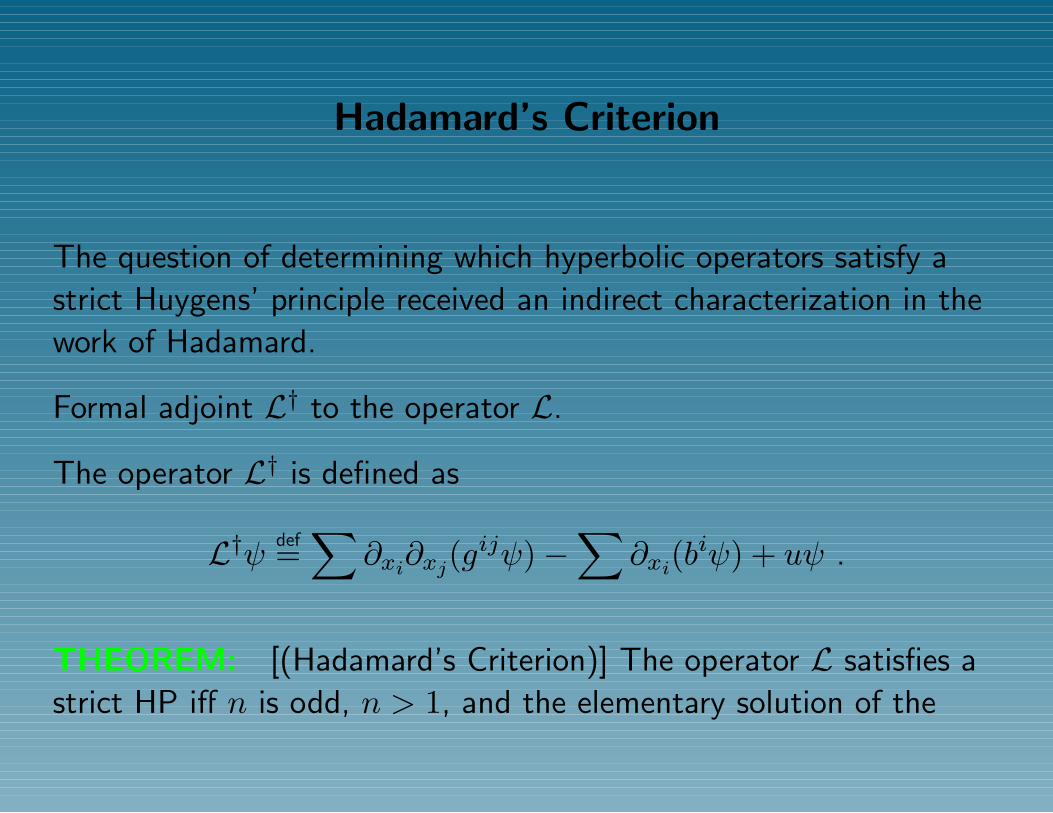
Hadamard’s Criterion
The question of determining which hyperbolic operators satisfy a
strict Huygens’ principle received an indirect characterization in the
work of Hadamard.
Formal adjoint L† to the operator L.
The operator L† is defined as
L†ψ def=∑
∂xi∂xj(gijψ)−
∑∂xi(b
iψ) + uψ .
THEOREM: [(Hadamard’s Criterion)] The operator L satisfies a
strict HP iff n is odd, n > 1, and the elementary solution of the
adjoint operator L† contains no logarithmic term, i.e., W0(x, ξ) = 0for all ξ and all x in the internal part of the characteristic conoid.

adjoint operator L† contains no logarithmic term, i.e., W0(x, ξ) = 0for all ξ and all x in the internal part of the characteristic conoid.
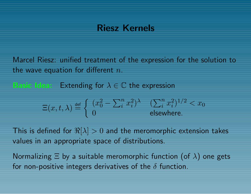
Riesz Kernels
Marcel Riesz: unified treatment of the expression for the solution to
the wave equation for different n.
Basic Idea: Extending for λ ∈ C the expression
Ξ(x, t, λ) def=
(x20 −
∑ni x
2i )λ (
∑ni x
2i )
1/2 < x0
0 elsewhere.
This is defined for <[λ] > 0 and the meromorphic extension takes
values in an appropriate space of distributions.
Normalizing Ξ by a suitable meromorphic function (of λ) one gets
for non-positive integers derivatives of the δ function.
A Few Technicalities
g a Lorentzian metric of signature +,−,−, . . . ,−.
Square of the geodesic distance Υ(x, ξ),
Characteristic conoid C(ξ), by the equation Υ(x, ξ) = 0.
C(ξ) \ ξ: two connected components C+(ξ) and C−(ξ), which are
naturally associated with the forward and backward time.
Open subsets of Ω as D+(ξ) and D−(ξ).
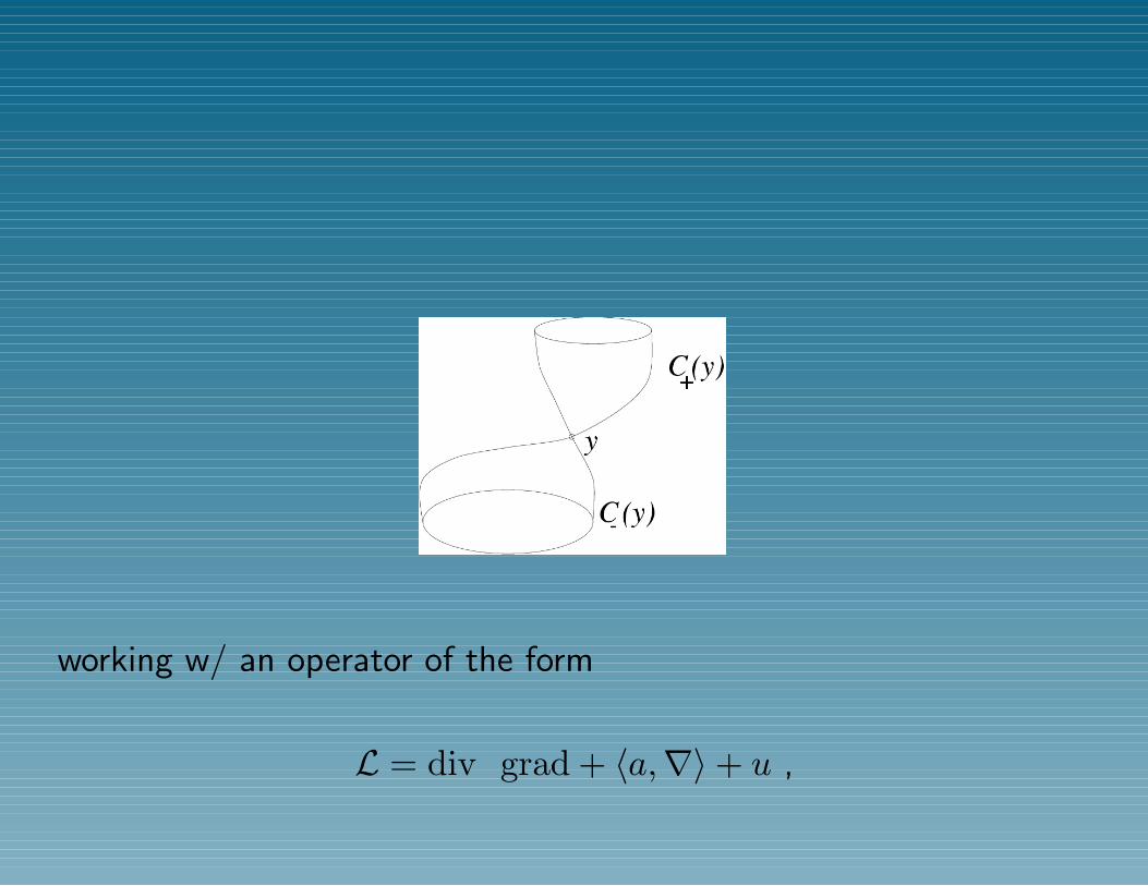
working w/ an operator of the form
L = div grad + 〈a,∇〉+ u ,
all coefficients (real) analytic and defined in a causal domain Ω.
Causal Domain:
1. Any two pts x and ξ are joined by a unique geodesic.
2. D+(x) ∩D−(ξ) is either empty or compact in Ω.
DEFINITION
A forward Riesz kernel of L is a holomorphic mapping
C 3 λ 7→ ΦΩλ(·, ξ) ∈ D′(Ω) ,
s.t.
supp[ΦΩλ(·, ξ)] ⊆ D+(ξ) (37)
L[ΦΩλ(·, ξ)] = ΦΩ
λ−1(·, ξ) (38)
ΦΩ0 (·, ξ) = δξ . (39)
Remarks:
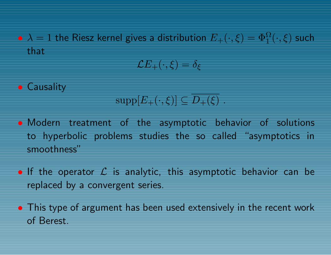
• λ = 1 the Riesz kernel gives a distribution E+(·, ξ) = ΦΩ1 (·, ξ) such
that
LE+(·, ξ) = δξ
• Causality
supp[E+(·, ξ)] ⊆ D+(ξ) .
• Modern treatment of the asymptotic behavior of solutions
to hyperbolic problems studies the so called “asymptotics in
smoothness”
• If the operator L is analytic, this asymptotic behavior can be
replaced by a convergent series.
• This type of argument has been used extensively in the recent work
of Berest.
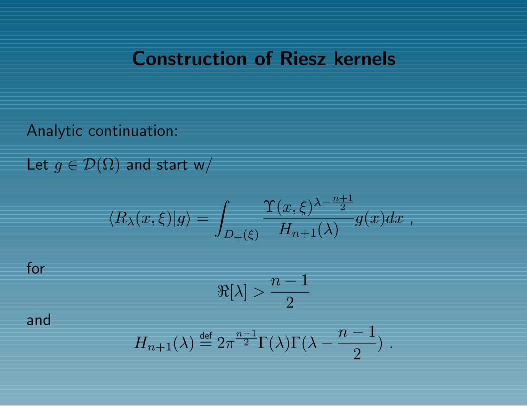
Construction of Riesz kernels
Analytic continuation:
Let g ∈ D(Ω) and start w/
〈Rλ(x, ξ)|g〉 =∫D+(ξ)
Υ(x, ξ)λ−n+1
2
Hn+1(λ)g(x)dx ,
for
<[λ] >n− 1
2and
Hn+1(λ) def= 2πn−1
2 Γ(λ)Γ(λ− n− 12
) .
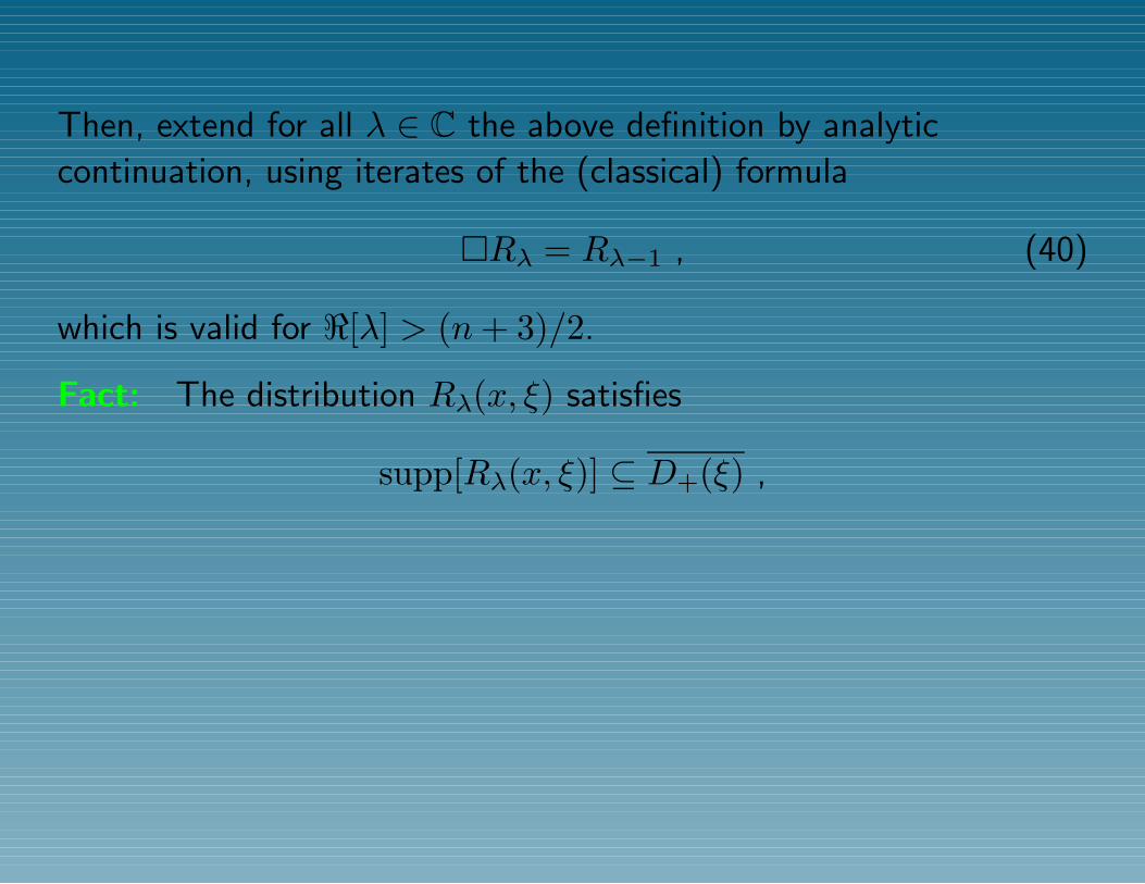
Then, extend for all λ ∈ C the above definition by analytic
continuation, using iterates of the (classical) formula
Rλ = Rλ−1 , (40)
which is valid for <[λ] > (n+ 3)/2.
Fact: The distribution Rλ(x, ξ) satisfies
supp[Rλ(x, ξ)] ⊆ D+(ξ) ,
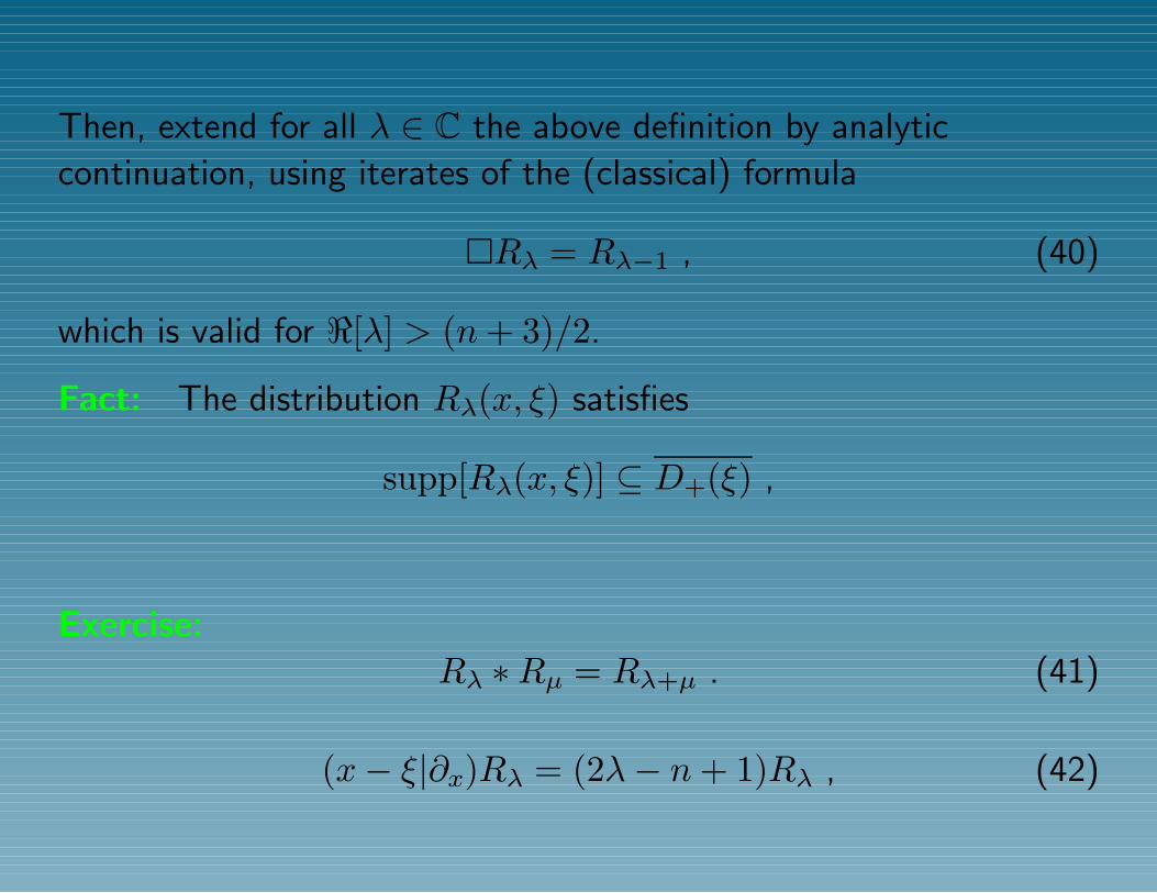
Then, extend for all λ ∈ C the above definition by analytic
continuation, using iterates of the (classical) formula
Rλ = Rλ−1 , (40)
which is valid for <[λ] > (n+ 3)/2.
Fact: The distribution Rλ(x, ξ) satisfies
supp[Rλ(x, ξ)] ⊆ D+(ξ) ,
Exercise:Rλ ∗Rµ = Rλ+µ . (41)
(x− ξ|∂x)Rλ = (2λ− n+ 1)Rλ , (42)
R0(x, ξ) = δξ(x) , (43)
Proposition: For an odd n λ ∈ 1, 2, . . . , (n− 1)/2 we have
Rλ(x, ξ) =δ
(n+12 −λ)
+ (Υ)βn,λ
, (44)
where δ+(Υ) stands for the the Dirac’s delta measure concentrated
on C+(ξ) ∩ Υ = 0, and βn,λ a numerical constant.
Now, look for an expansion of the fundamental solution
E(x, ξ) ∼∞∑ν=0
Uν(x, ξ)Rλ+ν(x, ξ) . (45)
Substitute expression (45) into
LE = δξ
obtain a set of recursive transport relations
(x− ξ|∂x)Uν(x, ξ) + νUν(x, ξ) = −14L[Uν−1(x, ξ)] . (46)
Facts:
• The above recursive system has a unique solution provided one
normalizes
U0(x, ξ) = 1 , (47)
and requires for r ≥ 1
Ur(x, ξ) = O(1) , x→ ξ . (48)
• If the operator L has analytic coefficients, then the series (46) is
uniformly convergent in a sufficiently small neighborhood of Υ = 0.
Riesz kernel for the operator L can be expanded as
ΦΩλ(x, ξ) =
∞∑ν=0
4νΓ(λ+ ν)
Γ(λ)Uν(x, ξ)Rλ+ν(x, ξ) .
Main argument for the proof of Hadamard’s result:
If n is even then for ν = 0, 1, 2, . . . we have
supp[Rν+1(x, ξ)] = D+(ξ) ,
and so Huygens principle does not hold.
If n is odd then for ν = 0, 1, 2, . . . , (n− 3)/2 we have
supp[Rν+1(x, ξ)] = C+(ξ) .
Notice: Using equation (46), and p = (n− 1)/2 one gets
Hadamard’s classical formula for n odd
E+(x, ξ) =1
2πp(V (x, ξ)δ(p−1)
+ (Υ) +W (x, ξ)H+(Υ)) ,
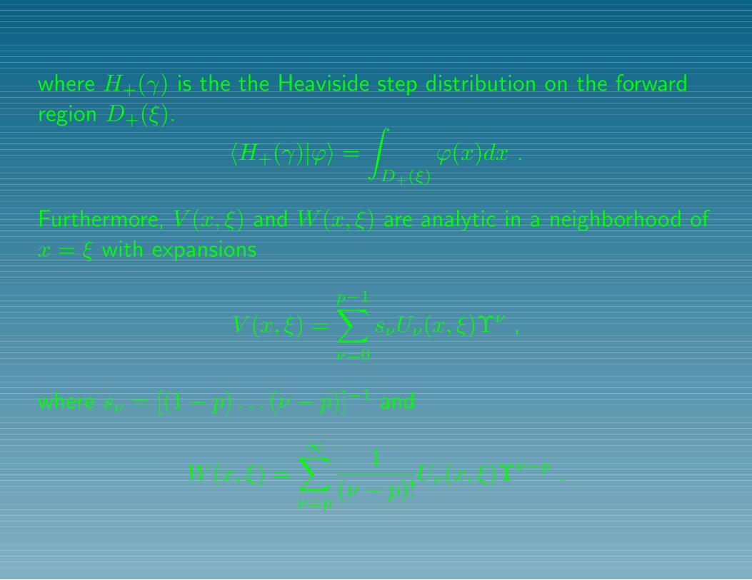
where H+(γ) is the the Heaviside step distribution on the forward
region D+(ξ).
〈H+(γ)|ϕ〉 =∫D+(ξ)
ϕ(x)dx .
Furthermore, V (x, ξ) and W (x, ξ) are analytic in a neighborhood of
x = ξ with expansions
V (x, ξ) =p−1∑ν=0
sνUν(x, ξ)Υν ,
where sν = [(1− p) . . . (ν − p)]−1 and
W (x, ξ) =∞∑ν=p
1(ν − p)!
Uν(x, ξ)Υν−p .
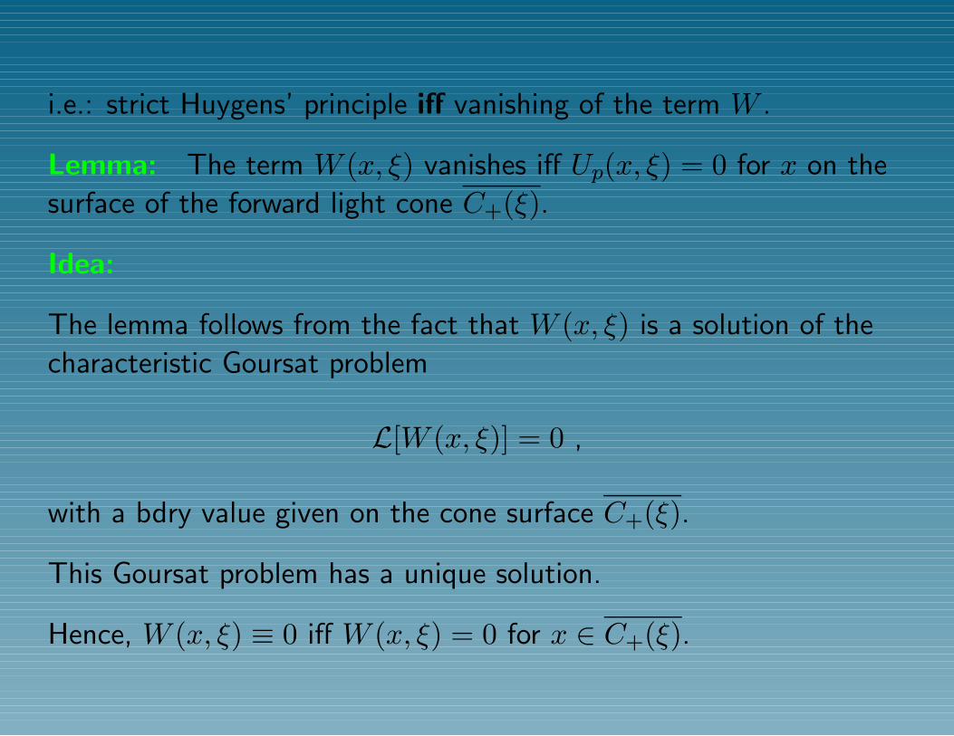
i.e.: strict Huygens’ principle iff vanishing of the term W .
Lemma: The term W (x, ξ) vanishes iff Up(x, ξ) = 0 for x on the
surface of the forward light cone C+(ξ).
Idea:
The lemma follows from the fact that W (x, ξ) is a solution of the
characteristic Goursat problem
L[W (x, ξ)] = 0 ,
with a bdry value given on the cone surface C+(ξ).
This Goursat problem has a unique solution.
Hence, W (x, ξ) ≡ 0 iff W (x, ξ) = 0 for x ∈ C+(ξ).
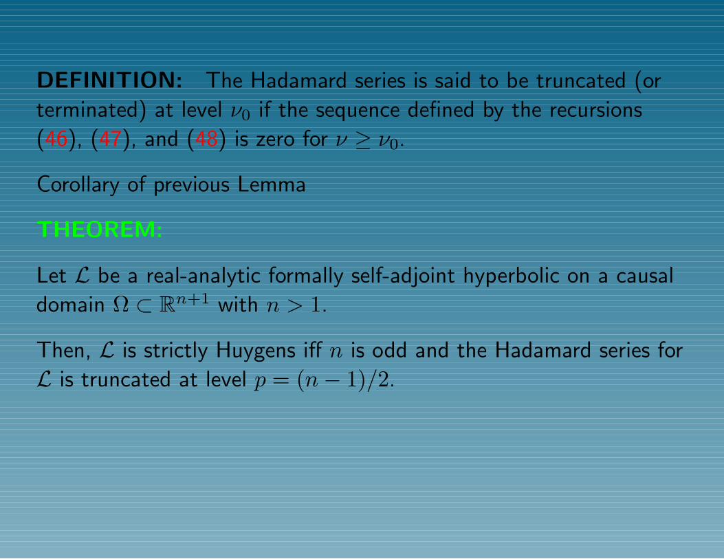
DEFINITION: The Hadamard series is said to be truncated (or
terminated) at level ν0 if the sequence defined by the recursions
(46), (47), and (48) is zero for ν ≥ ν0.
Corollary of previous Lemma
THEOREM:
Let L be a real-analytic formally self-adjoint hyperbolic on a causal
domain Ω ⊂ Rn+1 with n > 1.
Then, L is strictly Huygens iff n is odd and the Hadamard series for
L is truncated at level p = (n− 1)/2.
References
[1] J. J. Duistermaat and F. A. Grunbaum. Differential equations in
the spectral parameter. Comm. Math. Phys., 103(2):177–240,
1986.
[2] J. P. Zubelli and F. Magri. Differential equations in the spectral
parameter, Darboux transformations, and a hierarchy of master
symmetries for KdV. Commun. Math. Phys., 141(2):329–351,
1991.
[3] Jorge P. Zubelli. Rational solutions of nonlinear evolution
equations, vertex operators, and bispectrality. J. Differential
Equations, 97(1):71–98, 1992.
[4] Jorge P. Zubelli and D.S. Valerio Silva. Rational solutions of
the master symmetries of the KdV equation. Commun. Math.
Phys., 211(1):85–109, 2000.
[5] George Wilson. Collisions of Calogero-Moser particles and an
adelic Grassmannian (with an appendix by I. G. Macdonald).
Invent. Math., 133(1):1–41, 1998.