Hybrid Approach for Short-Term Traffic State and Travel

60

Transportation Research Record: Journal of the Transportation Research Board, No. 2554, Transportation Research Board, Washington, D.C., 2016, pp. 60–68.DOI: 10.3141/2554-07

Traffic management and traffic information are essential in urban areas and require reliable knowledge about the current and future traf-fic state. Parametric and nonparametric traffic state prediction tech-niques have previously been developed with different advantages and shortcomings. While nonparametric prediction has shown good results for predicting the traffic state during recurrent traffic conditions, para-metric traffic state prediction can be used during nonrecurring traffic conditions, such as incidents and events. Hybrid approaches have pre-viously been proposed; these approaches combine the two prediction paradigms by using nonparametric methods for predicting boundary conditions used in a parametric method. In this paper, parametric and nonparametric traffic state prediction techniques are instead combined through assimilation in an ensemble Kalman filter. For nonparametric prediction, a neural network method is adopted; the parametric pre-diction is carried out with a cell transmission model with velocity as state. The results show that the hybrid approach can improve travel time prediction of journeys planned to commence 15 to 30 min into the future, with a prediction horizon of up to 50 min ahead in time to allow the journey to be completed.

Traffic management and traffic information are essential in urban areas. Reliable knowledge about the current and future traffic state is required. Today, the road infrastructure in urban areas is commonly equipped with different types of sensors, capturing speed, flows, and travel time data. Using these data for traffic state estimation is a well-studied area and involves data-filtering techniques and traf-fic simulation models. Examples of filtering approaches for traffic state estimation can be found elsewhere (1–4) as can traffic simu-lation approaches (5–9). With the deployment of traffic sensors of various kinds, it has become more important to combine these two approaches (10–12).

While traffic state prediction in general is based on the current traffic state estimate, it is usually considered to be a more complex problem than estimating the traffic state since the future is always

unknown. The literature consists of several examples of applica-tions for traffic state prediction. First and most important, it is a critical component for real-time traffic control and management; see for example, Chen and Grant-Muller (13), Bajwa et al. (14), van Lint et al. (15), and Wang et al. (16). The ability to accurately predict the traffic state could increase the traffic manager’s ability to take action before the system reaches congestion and then at least forestall that event.

Common nonparametric methods for traffic state and travel time estimation are linear time series, k–nearest neighbors, locally weighted regression, fuzzy logic, Bayesian networks, and neural networks. For an overview of commonly used methods, see, for example, van Hinsbergen et al. (17). In nonparametric models, parameters and the structure of the model need to be determined from data. Such models are created from a large amount of historical data. They can capture the traffic dynamics even though no knowledge of the traffic pro-cesses as such is needed. Nonparametric models all inherit the prop-erty that only traffic states that already occurred can be predicted. Thus, they are appropriate for predicting recurring traffic conditions, but less appropriate for nonrecurring traffic conditions.

Several examples of parametric models can be applied for the purpose of traffic state prediction. Such examples include the micro-scopic simulation approach in Ben-Akiva et al. (5) and Torday (9), the mesoscopic simulation approach in Mahmassani et al. (6), and the macroscopic traffic flow models in Meschini and Gentile (7) and Papageorgiou et al. (8). Common for all these models is that they include parameters with a predetermined structure. Still, these param-eters need to be calibrated according to empirical data. Parametric models all inherit the property of describing only traffic phenom-ena that follow from the predetermined relationship between model parameters. Also, they rely on boundary conditions, such as traffic demand, which need to be predicted for the entire prediction horizon.

One way of approaching the shortcomings of nonparametric and parametric models is to combine them in a hybrid model approach (18). This is, for example, done in Calvert et al. (19) and Pan et al. (20) with nonparametric models for predicting demand profiles to be used in a parametric model. Accurate measurements of inflows at on-ramps and outflows at off-ramps will be required, however, and this information can be difficult to obtain.

For real-time traffic state estimation purposes, output from a parametric model is assimilated with live sensor data in Work et al. with a Kalman filtering approach (11). In this paper, the use of this approach will be extended to traffic state prediction. The result is a novel hybrid model using the filter for assimilating parametric traffic state prediction output with nonparametric prediction of the

Hybrid Approach for Short-Term Traffic State and Travel Time Prediction on Highways

Andreas Allström, Joakim Ekström, David Gundlegård, Rasmus Ringdahl, Clas Rydergren, Alexandre M. Bayen, and Anthony D. Patire

A. Allström, J. Ekström, D. Gundlegård, R. Ringdahl, and C. Rydergren, Department of Science and Technology, Linköping University, Bredgatan 33, Norrköping SE-601 74, Sweden. A. M. Bayen, 710 Davis Hall, and A. D. Patire, 410-2 McLaughlin Hall, Department of Civil and Environmental Engineering, College of Engineering, Univer-sity of California, Berkeley, CA 94720. Corresponding author: J. Ekström, joakim [email protected].

Allström, Ekström, Gundlegård, Ringdahl, Rydergren, Bayen, and Patire 61

point speed at several radar sensor locations. Thus, errors from demand profiles based on uncertain measurements can be compen-sated for with the use of point speed predictions at main-line sensor locations, which are based on more reliable speed measurements.

As a parametric model, the cell transmission model (CTM) will be used with velocity as state (CTM-v), which is a macroscopic traffic flow model from the family of cell transmission models (11). This family includes several models that have previously been applied suc-cessfully for traffic state estimation on highways. For nonparametric prediction, neural networks will be used; these have been shown to be a powerful tool for nonparametric traffic state, travel time, and demand profile prediction (21–23). The contribution of this paper is not, however, in the development of parametric and nonparametric models, but in the way they are combined in the hybrid framework.

The rest of this paper is organized as follows. The hybrid model-ing framework is presented, including the macroscopic flow model and the Kalman filter. Next, the experimental setup is introduced and the results are presented for a 7-km-long section of the Stockholm, Sweden, ring road, followed by final conclusions and suggestions for future work.

Hybrid Prediction Framework

macroscopic Flow model

The traffic state estimation and prediction will be based on the CTM-v, which is a first order traffic model developed from the density-based cell transmission model (CTM-ρ). The CTM-ρ model is, in turn, based on the Godunov discretization of the well-known Lighthill–Whitham–Richards model (24). It is possible to directly formulate a velocity-based version of that model, but the resulting partial differential equation can be solved numerically only if the relationship between speed and density is assumed to be affine. Therefore the transfor-mation from density to velocity in the CTM-v is done within the discretization scheme.

In the CTM-v, the traffic state is discretized into cells, and for each cell the velocity is used as the traffic state. At each time step, the Lighthill–Whitham–Richards partial differential equation is solved numerically with the use of the CTM-v. For each cell, the relation-ship between speed, v, and density, ρ, is given by a fundamental diagram, v = V(ρ). Using the velocity as state makes it easy to com-bine the model output with actual speed measurements from traffic detectors. This feature is the main reason for adopting the CTM-v rather than the CTM-ρ. The CTM-v, however, requires the velocity function to be strictly decreasing and invertible. Thus, the commonly applied Daganzo–Newell fundamental diagram cannot be used and instead a hyperbolic–linear velocity function is adopted with a linear expression in free flow and a hyperbolic expression in congestion

v V

v

w

f

f

1 if

1 otherwise

maxcr

max

( )= ρ =

−ρ

ρ

ρ ≤ ρ

− −ρ

ρ

where

ρmax = jam density, vf = free-flow speed, wf = backward propagating shock wave speed, and ρcr = critical density.

The demand is specified in regard to inflow rates and split ratios at diverging nodes. Inflow rates are considered as boundary condi-tions to the CTM-v, and the split ratios are specified as parameters in the model. For a comprehensive description of the CTM-v, see Work et al. (11).

traffic State estimation Using ensemble kalman Filtering

As the basis for the traffic state and travel time prediction, the current traffic state needs to be estimated. The data fusion model, developed in the Mobile Millennium project and described in Work et al. (11) and Bayen et al. (25), is appealing for many reasons. First, it is devel-oped to run in real time and for a large network. Furthermore, it can fuse different types of point speed measurements, but the Kalman fil-ter also provides the possibility to include travel time measurements (26). The state–space model of the system is formulated as

( )

( )

( )

( )

= + η

= + χ

η ∝ µ

χ ∝ µ

−v M v

y h v

Q

R

n n n

kn

kn

kn

n n

kn

kn

,

,

1

mod

obs

where

vn = state vector in time step n, including speed for each part of road network (cell) according to spatial resolution of system;

M(•) = system model, here CTM-v model; yn = observation vector in time step n; hk(•) = observation model for observation type k; and η and χ = possibly time-varying model uncertainty (with mean

µmod and covariance Q) and observation noise (with µobs and covariance R), respectively.

A number of different adaptions and extensions to the Kalman filter have been proposed over the years. The basic Kalman filter is designed for linear problems, but the extension of the CTM-v to networks implies a nonlinear and nondifferentiable state equation. Different extensions to the Kalman filter can manage nonlinearity; one commonly used example is the extended Kalman filter that has been used for traffic estimation by Wang and Papageorgiou and others (27). However, in the extended Kalman filter all functions have to be differentiable, which is not the case for CTM-v. An alternative to the extended Kalman filter is the ensemble Kalman filter (EnKF). The EnKF, first presented by Evensen (28), is an extension of the classical Kalman filter that has shown good performance also for nonlinear dynamical models (29) and can handle nondifferentia-bility. The EnKF belongs to a class of particle methods that use Monte Carlo representation of the probability density functions and their time evolution and can be viewed as a combination of the Kalman filter and the particle filter.

In the EnKF, the state estimate distribution—the error covariance matrix—is represented as a set of ensembles that makes it suitable for problems with a large state vector, such as traffic state estima-tion for large networks. The ensemble of model states is propa-gated forward in time, making it possible to calculate the mean and

62 Transportation Research Record 2554

covariance of the error needed in the measurement update step. Although the EnKF uses Gaussian assumption on the probability density functions, the integration of ensembles through the model will inherit important characteristics of potentially non-Gaussian probability density functions, as well as nonlinearity in the model. See Evensen for a detailed description of the EnKF (28).

The traffic state estimation framework is presented in Figure 1. Currently only data from fixed sensors are available in the Stockholm area. These data are preprocessed and later assimilated with the CTM-v every 60 s. The framework, however, supports multiple data sources as is illustrated, including probe data [e.g., data collected with GPS probes (30)].

Prediction Framework

The traffic state prediction framework involves components similar to those of the estimation framework presented in the previous sec-tion and is illustrated in Figure 2. Starting from a known traffic state (given by the most recent estimation) and predicted inflows and split ratios, the CTM-v can be run forward in time from a known traffic state estimation. Prediction of inflows and split ratios can be done either with nonparametric methods, as is done in Calvert et al. (19), Pan et al. (20), and Wu et al. (31), or by simple averaging of his-torical data. Accurate measurements of inflow rates and split ratios can be difficult to obtain during congested periods. Curbside driving together with blocking back of either the main line or the ramps may, for example, result in measurements that do not represent the actual inflow and split ratio profiles. Also, as is pointed out in Wu et al., main-line flows are actually aggregations of upstream on-ramp flows and main-line sensor measurements, and thus have a reduced noise (31). This aspect makes nonparametric prediction of main-line flows more accurate in comparison with predictions of on-ramp flows.

It is also possible to combine the CTM-v model with nonparamet-ric prediction of the main-line sensor data through the EnKF. This combination results in an alternative hybrid traffic state prediction. Thus, it is possible to take advantage of the parametric and non-parametric prediction methods. With EnKF parameters to govern the influence of each method, either the parametric or nonparamet-

ric prediction can be trusted more or less depending on the current traffic situation. As an example, the nonparametric method may be more trustworthy during recurring congestion situations, and the parametric estimation more reliable when there are nonrecurring events, such as incidents, which can be modeled as reduced capaci-ties in the CTM-v. The introduction of predicted sensor data in the EnKF, however, introduces additional filter parameters related to predicted measurement uncertainty, which need to be calibrated.

Prediction of sensor data to be used in the hybrid prediction can be done with a number of nonparametric methods. Here, a non linear autoregressive neural network with an exogenous input (NARX) model will be used. Such a model is commonly used for short-term predictions based on time series analysis and can include time delay of inputs as well as time-delayed feedback loops of outputs. In Zeng and Zhang, such a model is successfully applied for travel time pre-

FIGURE 1 Traffic state estimation framework.

FIGURE 2 Prediction framework.


dictions on a freeway (32). A similar approach is the state–space neural network, applied in van Lint et al. for prediction of travel times using travel times and flows from fixed traffic sensors as input (15).

The input for predicting speeds at a specific sensor with the NARX neural network will be speeds measured at the specific main-line sen-sor location, as well as speeds from the surrounding sensors. The NARX model will include time-delayed inputs, as well as time-delayed feedback of outputs. Thus, the predictions will be based not only on the most recent measurements, but also on the trend from several recent measurements and on time of day and day of week (clustered in Mondays to Thursdays as one cluster, and Fridays and weekend days as their own clusters). Outputs are the speeds for coming time periods at sensor locations.

The setups of the parametric and nonparametric estimation methods are further described in the next section.

exPerimental SetUP

Stockholm test Site

To analyze the prediction framework a section of the highway just north of central Stockholm will be studied. The section is 7 km long and part of the southbound Stockholm ring road. Data from January to March 2013 are used, and for this period radar detector data were available. During March, Bluetooth sensor data were also available. The radar detectors collected speed and flow for each lane, aggre-gated at 1-min intervals, and are illustrated in Figure 3. Bluetooth sensors are placed every 500 to 1,000 m and collect travel times from all active Bluetooth units that pass two consecutive sensors. The sections with Bluetooth measurements are marked in Figure 3 with BT1 up to BT7, together with the length of each section. There are three on-ramps and three off-ramps in the studied section, and the number of lanes varies between two and four. Bluetooth data were available only for a limited number of days and had been used only for calibration of EnKF parameters and for validation of the results presented in this paper.

In Figure 3, radar sensors with available data are marked with “+”. For sensors that are used for the nonparametric prediction, sensor IDs are included for future reference.

Setup and calibration of ctm-v model

Speeds and flow measurements from 23 days (only Mondays to Fridays were selected) have been used for calibrating the funda-

mental diagrams as well as the inflow at on-ramps and split ratios at diverging nodes.

For cells in each of the marked sections in Figure 3, the same fun-damental diagram is used. All fundamental diagrams are specified with the same jam density, which is measured from aerial photos over the Stockholm highway system (33). Free-flow speed has been measured with data from Bluetooth sensors. The most downstream section is a bottleneck, which is usually activated during the morn-ing and afternoon peak periods. Capacity measurements have been used for calibrating the shockwave speed (given jam densities and free-flow travel times) for the bottleneck. For the remaining sec-tions, standard capacities have been applied from Olstam et al., with manual adjustments for the merging sections to achieve a better fit between model output and measured data (34).

Profiles with daily variations of inflows and split ratios are con-structed by taking mean values for 15-min periods from the 23 days used for calibrations. For the most upstream on- and off-ramp, these profiles are computed by comparing the flow before and after the on- and off-ramp, respectively. For the remaining on-ramps, the inflows were measured on the ramp itself; and for the split ratios, flow measurements from the main-line and off-ramp sensors were compared. In the presence of queues, this computation of inflow and split ratios introduces potential errors. The measured split ratios may be an effect of the main-line lane functioning as an extended ramp, and the inflows may be restricted by the blocking back of queues from the main line. This information is the best information available.

Sink capacities can be used for restricting the outflow, marked by outflow arrows. If the outflow exceeds the sink capacity, the flow will block back. This can be used to model capacities in the sur-rounding network or to model blocking back from the surrounding network. For the studied highway section, sink capacities are set only for the outflow at the most downstream subsection since blocking back from the remaining network is an issue mainly in this sub-section. The sink capacity is lower than the bottleneck capacity only at the most downstream section during the afternoon. A sink capac-ity, as well as the start and end times of the reduced capacity period, has been calibrated on the basis of the 23 calibration days. The length of the afternoon congestion period and the maximum queue length have been the main comparisons used for this calibration. Overall, the afternoon is more difficult to model because of the blocking back from the remaining traffic network. Validation of the model has been done with data from March 21, and the resulting mean average per-centage error (MAPE)—as well as the mean and maximum errors—are presented in Table 1.

FIGURE 3 Stockholm test site (not to scale).


Prediction of Sensor data

The nonparametric prediction of speeds at radar sensor locations using the NARX neural network is done for Sensors 230, 231, 235, 236, 238, 239, and 244. These predictions will be referred to as “predictions of measurements.” The time resolution of the predicted measurements is important to capture changes in the traffic state. A prediction horizon of 1 h is used, and for the first 10

min, measurements for 2-min periods are predicted on the basis of the mean speed measurements of all sensors for 2-min periods. For predictions 10 to 30 min ahead in time, a time resolution of 5-min periods is used; for 30 to 60 min ahead in the future, 10-min periods are used. Using a time delay of five periods in the NARX neural network, one looks 10 min back in time for prediction 10 min ahead, 25 min back when predicting 10 to 20 min ahead in time, and 50 min back when predicting 30 to 60 min ahead in time. The NARX neural network is set up with an output feed-back loop of the two most recent time periods and one layer with 10 neurons. Each time period results in a neural network to train, and 12 neural networks were trained for each sensor location, with hour of day and day of week (grouped into Monday to Thursday, Friday, and weekends), and speed measurements from all sensors. The training was done with 53 days during January, February, and March 2013.

MAPE values for predicted measurements on March 21, 2013, are presented in Table 2. The MAPE values are based on the dif-ference between predicted and measured mean values for 2-, 5-, and 10-min periods, depending on how far ahead in the future the prediction is. While the MAPE values are not necessarily increased when one predicts one time period further ahead in time, the overall trend is that uncertainty is increased when measurements are pre-dicted further ahead. Sensor 244 stands out with the lowest MAPE value; the reason is that there are very few time periods of day when the congestion reaches this sensor, and predicting speeds during noncongested traffic states has been shown to be much easier than to predict speeds during congested periods.

estimation and calibration of ensemble kalman Filter Parameters

The measurement noise is assumed to have zero mean, and the stan-dard deviation has been estimated to be 1 m/s from measurements. The model noise is assumed to have a zero mean and a standard deviation of 0.8 m/s. The model noise standard deviation has been calibrated with an evaluation of MAPE values between estimated and Bluetooth travel times for a number of different parameter settings. The resulting MAPE values are presented in Table 1.

Predicted measurement uncertainty was assumed to have a zero mean, and the initial guess of the standard deviation was to use the same as for the measurement noise. There is, however, an increased uncertainty in the predicted measurements, and the best result has been obtained with a standard deviation twice that of the measurement noise (2 m/s).

TABLE 1 Comparison of Predicted and Estimated Travel Times with Measured Travel Times

Prediction–Estimation Method

Horizon

0 5 15 30

MAPE Based on Subsection Travel Times (%)

Estimation 11.5 na

CTM-v 19.3

Naive prediction 13.8 14.7 18.5 27.0

CTM-v prediction 13.0 17.6 16.9 16.9

Hybrid prediction 13.0 15.7 15.3 16.6

MAPE Based on Total Subsection Travel Times (%)

Estimation 4.8 na

CTM-v 12.8


CTM-v prediction 5.1 9.2 10.1 10.9


Mean Absolute Error Based on Total Subsection Travel Times (s)

Estimation 22 na

CTM-v 56

Naive prediction 28 32 50 87

CTM-v prediction 25 45 48 49

Hybrid prediction 28 32 39 41

Maximum Absolute Error Based on Total Subsection Travel Times (s)

Estimation 205 na

CTM-v 378




Note: na = not applicable.

TABLE 2 MAPE for Predicted Measurements

Prediction Horizon Measured in Minutes Ahead in Time (%)

Sensor 1–2 3–4 5–6 7–8 9–10 11–15 16–20 21–25 26–30 31–40 41–50 51–60

230 4.41 4.51 4.77 4.60 4.76 5.61 5.12 5.44 5.42 7.10 7.35 7.48

231 6.05 6.17 6.37 6.55 6.50 7.41 7.62 7.65 7.98 8.46 9.23 10.23

235 6.15 5.65 6.21 6.15 6.09 6.71 7.11 7.00 6.36 11.51 13.01 11.42

236 4.91 4.99 6.38 5.03 6.08 6.82 5.93 6.20 5.97 11.88 13.59 11.89

238 4.70 4.27 5.11 4.88 5.23 7.52 7.01 7.28 7.08 14.69 16.56 15.26

239 4.46 4.35 4.80 4.54 4.67 5.69 6.17 5.97 6.89 9.97 10.07 9.16

244 2.73 2.84 2.92 2.78 2.79 3.29 3.28 3.18 3.06 4.56 4.86 4.98


evaluation of Prediction Framework

For evaluation of the hybrid prediction framework, results with data from March 21, 2013, will be presented. These data have not been used for either calibration or training purposes.

Speed maps will be used for comparing predictions of the traffic state—with and without measurements—with estimation results. Here, the estimation will be used as a reference (obtained by run-ning the EnKF framework) since it is the best available information according to all available sensor data and CTM-v output.

Travel times will be predicted for a car entering the highway at time t, by driving a car through the speed map corresponding to the prediction made at time t. Thus, this travel time prediction will make use of predicted traffic states ranging from 0 to 20 min ahead in the future, depending on how long it will take to drive through the evaluated highway section (i.e., depending on the level of congestion). Similarly, a travel time prediction for a car starting 30 min from now will make use of information from a prediction horizon ranging from 30 to 50 min into the future. As a comparison, a naive prediction, assuming the current traffic conditions will prevail during the next 60 min, is computed (resulting in an instantaneous travel time). The naive prediction makes use of only the most recent traffic state estima-tion. A MAPE value based on 5-min averaged travel times will be used for comparing the predicted travel times with the reference travel time obtained from driving a car through the estimation speed map. This comparison will be biased from the fact that the estimation may not correspond to the ground truth. Also, since the prediction is done for a car driving the whole section, predicted traffic states further ahead into the future will be used for predicting the later part of the journey in comparison with the early part of the journey. The size of this differ-ence depends on how long it will take for a driver to drive through the complete highway section and thus depends on the level of congestion.

To avoid the shortcomings of comparing predicted and estimated travel times, MAPE values of predicted travel times versus measured travel times (also for 5-min averages) measured with Bluetooth sen-sors are computed for seven subsections for which Bluetooth data exist. The seven subsections cover all but the last section of the high-way in Figure 3, and two different MAPE values based on the mea-surements will be computed. The first one is the mean error across all sections; for the other, the subsection travel times are added to provide a total travel time across all subsections. Thus, the latter will give approximate travel times for the seven subsections. For the total travel times, mean and maximum absolute errors are also provided. All errors computed between predicted and Bluetooth travel times will be based on cars starting at different locations (the beginning of each Bluetooth segment) of the highway at the same time. Each subsection is short, however, and thus predictions at most 35 min ahead into the future will be used.

The error values related to the estimation in Tables 1 and 3 are based on a car driving through the speed map corresponding to an estimation done after the arrival of the car. Thus, the estimation makes use of measurements that were not available at the time the car entered the section. In comparison, the naive prediction makes use of the most recent estimation and assumes prevailing traffic conditions during the time it takes to drive through the section.

reSUltS

Table 1 shows the MAPE as well as the mean and maximum abso-lute error value for comparison of the predicted travel times with measured travel times. For comparison, these error values for the

prediction done by running only the CTM-v with boundary condi-tions but not using the EnKF framework are also provided. The entry marked “estimation” is not a prediction but based on the real-ized travel times as given by the estimation framework. Similarly “CTM-v” refers to the case using the CTM-v with the historical boundary conditions only. In the other three methods, the predic-tion is always started from the current estimation (denoted “naive prediction,” “CTM-v prediction,” and “hybrid prediction”). Table 3 shows the same error values for the comparison of predicted travel times with estimated travel times.

The three prediction methods, which are based on the most recent estimation plus a prediction, show similar results for a car starting its journey at the time of the prediction when compared with the Bluetooth reference travel times. For a journey taking place 15 and 30 min ahead in time, the hybrid prediction is the best-performing prediction considering subsection MAPE values although the dif-ferences are rather small when compared with the CTM-v predic-tion. For the case of a prediction 30 min ahead in time, the naive prediction performs worse than the CTM-v. Considering the total travel time in Table 2, the hybrid prediction results in the lowest maximum absolute error values for all prediction horizons, but for predictions far ahead into the future, it tends to the same value as the CTM-v prediction. This finding could be related to the quality of the predicted measurements being less reliable for predictions further ahead in time.

When comparing against estimated reference travel times, the hybrid prediction is the best-performing one from a mean value per-spective, for all time horizons. For a worst-case scenario, the hybrid prediction performs best for a journey taking place 15 and 30 min ahead in time, and the CTM-v prediction performs best for jour-neys taking place 0 and 5 min ahead. For the prediction of journeys taking place up to 15 min ahead, the differences between all three approaches are quite small. The major difference appears for a journey taking place 30 min ahead, for which the naive prediction performs poorly, but for which the CTM-v and hybrid predictions have similar results as for a journey taking place 15 min ahead in time.

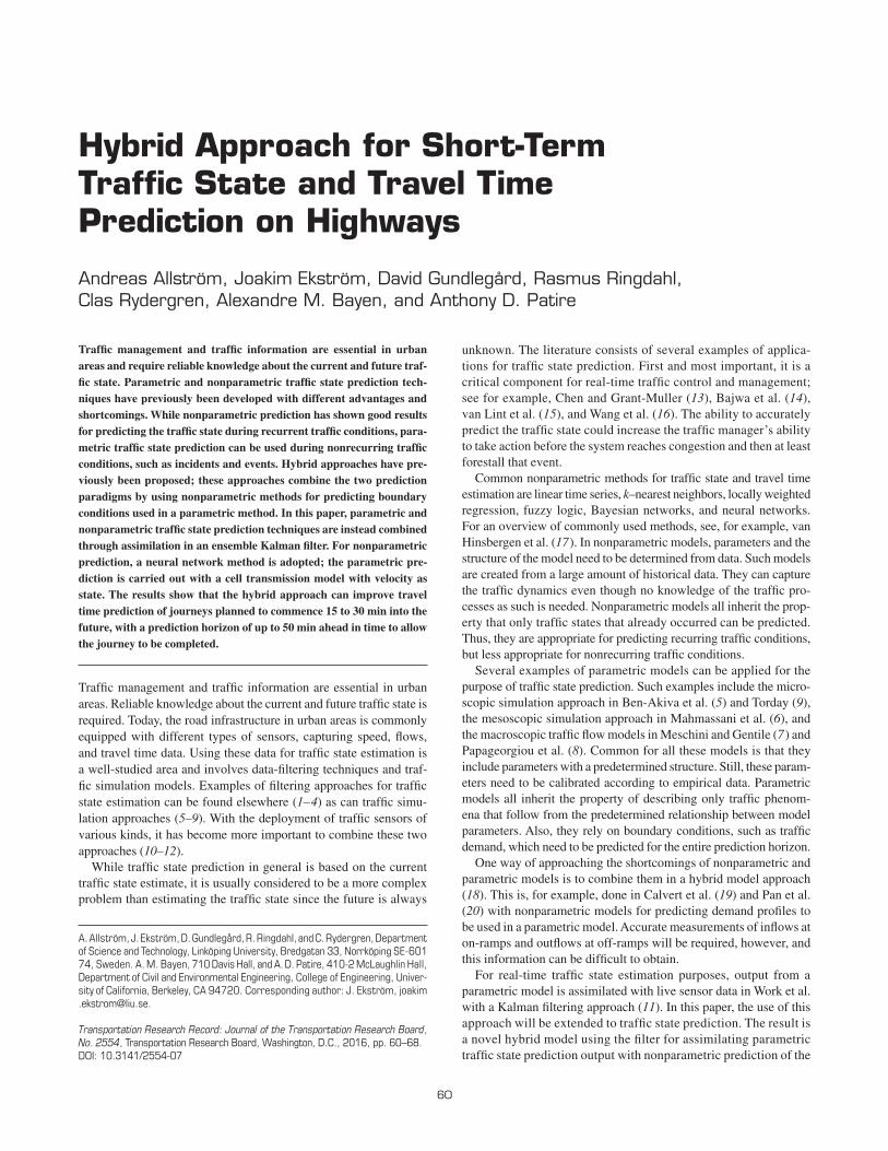
In Figure 4, the estimated and predicted travel times are shown for a journey taking place at the time of the prediction and for journeys

TABLE 3 Comparison Between Estimated and Predicted Travel Times

Horizon

Prediction Method 0 5 15 30

MAPE (%)


CTM-v prediction 3.9 5.7 7.1 8.4


Mean Absolute Error (s)




Maximum Absolute Error (s)





(a)

20006:00 09:00 12:00

Time

15:00 18:00 21:00

400

600

800

1,000

Tra

vel T

ime

(s)

1,200

1,400

1,600

(b)

006:00 09:00 12:00

Time

15:00 18:00 21:00

500

1,000

Tra

vel T

ime

(s)

1,500

(c)

006:00 09:00 12:00

Time

15:00 18:00 21:00

500

1,000

Tra

vel T

ime

(s)

1,500

(d)

006:00 09:00 12:00

Time

15:00 18:00 21:00

500

1,000

Tra

vel T

ime

(s)

1,500

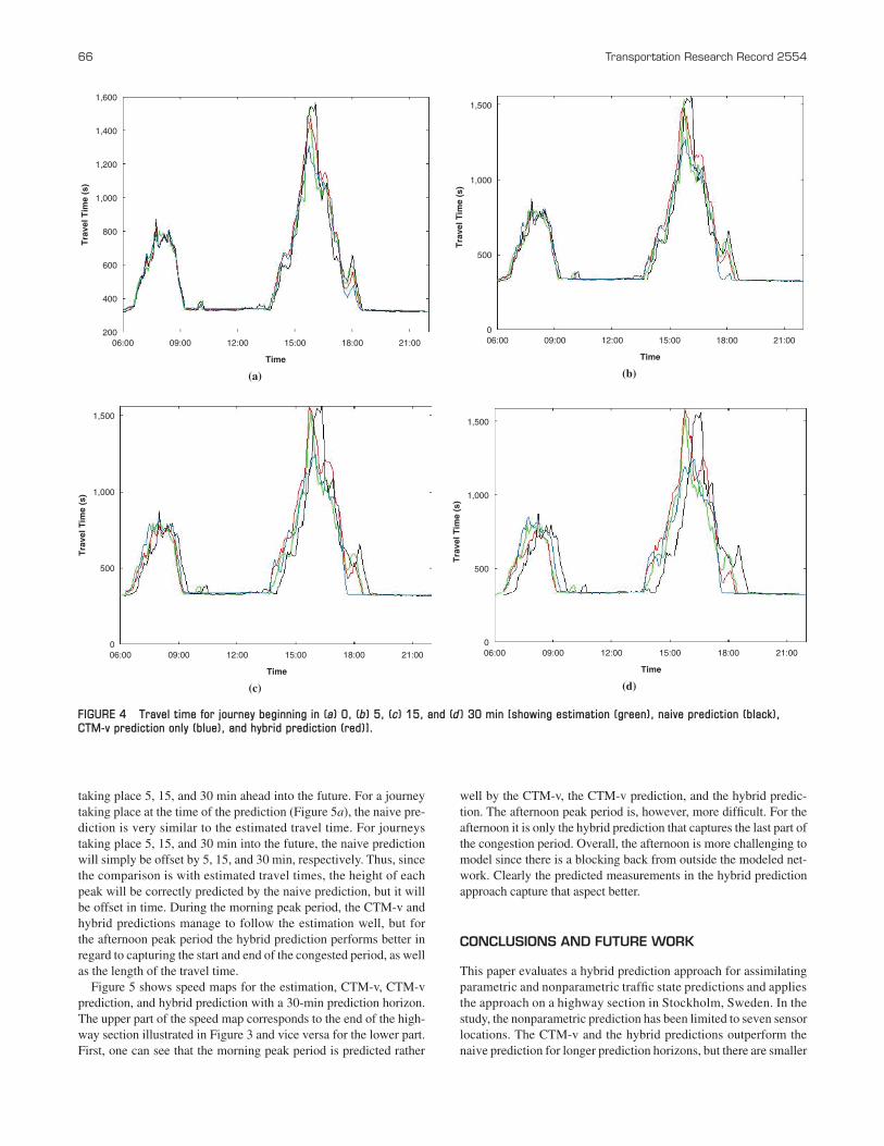
FIGURE 4 Travel time for journey beginning in (a) 0, (b) 5, (c) 15, and (d ) 30 min [showing estimation (green), naive prediction (black), CTM-v prediction only (blue), and hybrid prediction (red)].

taking place 5, 15, and 30 min ahead into the future. For a journey taking place at the time of the prediction (Figure 5a), the naive pre-diction is very similar to the estimated travel time. For journeys taking place 5, 15, and 30 min into the future, the naive prediction will simply be offset by 5, 15, and 30 min, respectively. Thus, since the comparison is with estimated travel times, the height of each peak will be correctly predicted by the naive prediction, but it will be offset in time. During the morning peak period, the CTM-v and hybrid predictions manage to follow the estimation well, but for the afternoon peak period the hybrid prediction performs better in regard to capturing the start and end of the congested period, as well as the length of the travel time.

Figure 5 shows speed maps for the estimation, CTM-v, CTM-v prediction, and hybrid prediction with a 30-min prediction horizon. The upper part of the speed map corresponds to the end of the high-way section illustrated in Figure 3 and vice versa for the lower part. First, one can see that the morning peak period is predicted rather

well by the CTM-v, the CTM-v prediction, and the hybrid predic-tion. The afternoon peak period is, however, more difficult. For the afternoon it is only the hybrid prediction that captures the last part of the congestion period. Overall, the afternoon is more challenging to model since there is a blocking back from outside the modeled net-work. Clearly the predicted measurements in the hybrid prediction approach capture that aspect better.

conclUSionS and FUtUre work

This paper evaluates a hybrid prediction approach for assimilating parametric and nonparametric traffic state predictions and applies the approach on a highway section in Stockholm, Sweden. In the study, the nonparametric prediction has been limited to seven sensor locations. The CTM-v and the hybrid predictions outperform the naive prediction for longer prediction horizons, but there are smaller


differences between the two approaches. Findings also suggest that the hybrid prediction is an improvement compared with the CTM-v prediction for all prediction horizons, especially for the afternoon peak, for which there are large uncertainties in the input flows, split ratios, and capacities used in the CTM-v model.

Overall the results are encouraging for continuing the work with the hybrid prediction approach. For further improvement the work should focus on

1. The combination of more advanced techniques for predicting inflows and split ratio, together with predicted measurements;

2. Calibration of EnKF parameters related to predicted measure-ment uncertainty;

3. Evaluation of alternative techniques for predicting measure-ments; and

4. Evaluation with an increased number of sensor locations used for the prediction of measurements.

acknowledgmentS

This research has been supported by the Swedish Transport Adminis-tration. The paper has benefited from the comments of five anonymous reviewers.

reFerenceS

1. Di, X., H. X. Liu, and G. A. Davis. Hybrid Extended Kalman Filtering Approach for Traffic Density Estimation Along Signalized Arterials. In Transportation Research Record: Journal of the Transportation Research Board, No. 2188, Transportation Research Board of the National Academies, Washington, D.C., 2010, pp. 165–173.

2. Schreiter, T., H. van Lint, M. Treiber, and S. Hoogendoorn. Two Fast Implementations of the Adaptive Smoothing Method Used in Highway Traffic State Estimation. Presented at 13th International IEEE Con-ference on Intelligent Transportation Systems (ITSC 2010), Madeira Island, Portugal, 2010, pp. 1202–1208.

FIGURE 5 Speed maps for (a) estimation and (b) CTM-v; 30-min predictions are presented for (c) CTM-v prediction and (d ) hybrid prediction (legend shows velocity in km/h).

Po

siti

on

(km

)

Time

(a)

Po

siti

on

(km

)

Time

(b)

Po

siti

on

(km

)

Time

(c)

Po

siti

on

(km

)

Time

(d)


3. Ngoduy, D. Low-Rank Unscented Kalman Filter for Freeway Traffic Estimation Problems. In Transportation Research Record: Journal of the Transportation Research Board, No. 2260, Transportation Research Board of the National Academies, Washington, D.C., 2011, pp. 113–122.

4. MacCarley, C., and E. Sandberg. Traffic Ground Truth Estimation Using Multisensor Consensus Filter. In Transportation Research Record: Journal of the Transportation Research Board, No. 2308, Transportation Research Board of the National Academies, Washington, D.C., 2012, pp. 128–137.

5. Ben-Akiva, M., M. Bierlaire, D. Burton, H. N. Koutsopoulos, and R. Mishalani. Network State Estimation and Prediction for Real-Time Traffic Management. Networks and Spatial Economics, Vol. 1, No. 3–4, 2001, pp. 293–318.

6. Mahmassani, H. S., X. Fei, S. Eisenman, X. Zhou, and X. Qin. DYNASMART-X Evaluation for Real-Time TMC Application: CHART Test Bed. Maryland Transportation Initiative, University of Maryland, College Park, 2005.

7. Meschini, L., and G. Gentile. Real-Time Traffic Monitoring and Fore-cast Through OPTIMA–Optimal Path Travel Information for Mobility Actions. In Proceedings of International Conference on Models and Technologies for Intelligent Transportation Systems (G. Fusco, ed.), Rome, 2009.

8. Papageorgiou, M., I. Papamichail, A. Messmer, and Y. Wang. Traffic Sim-ulation with Metanet. In Fundamentals of Traffic Simulation (J. Barceló, ed.), Springer, New York, 2010, pp. 399–430.

9. Torday, A. Simulation-Based Decision Support System for Real Time Traffic Management. Presented at 89th Annual Meeting of the Trans-portation Research Board, Washington, D.C., 2010.

10. Tampere, C. M. J., and L. H. Immers. An Extended Kalman Filter Application for Traffic State Estimation Using CTM with Implicit Mode Switching and Dynamic Parameters. Presented at 2007 IEEE Intelligent Transportation Systems Conference, Seattle, Wash., 2010, pp. 209–216.

11. Work, D., S. Blandin, O.-P. Tossavainen, B. Piccoli, and A. M. Bayen. A Traffic Model for Velocity Data Assimilation. Applied Mathematics Research eXpress, Vol. 2010, No. 1, 2010, pp. 1–35.

12. Antoniou, C., M. Ben-Akiva, and H. N. Koutsopoulos. Kalman Filter Applications for Traffic Management. In Kalman Filter (V. Kordic, ed.), InTech, Rijeka, Croatia, 2010, pp. 1–28.

13. Chen, H., and S. Grant-Muller. Use of Sequential Learning for Short-Term Traffic Flow Forecasting. Transportation Research Part C, Vol. 9, No. 5, 2001, pp. 319–336.

14. Bajwa, S. I., E. Chung, and M. Kuwahara. Performance Evaluation of an Adaptive Travel Time Prediction Model. In Proceedings of 2005 IEEE Intelligent Transportation Systems Conference, Piscataway, N.J., 2005, pp. 1000–1005.

15. van Lint, J. W. C., S. P. Hoogendoorn, and H. J. van Zuylen. Accurate Freeway Travel Time Prediction with State–Space Neural Networks Under Missing Data. Transportation Research Part C, Vol. 13, No. 5–6, 2005, pp. 347–369.

16. Wang, Y., M. Papageorgiou, and A. Messmer. Renaissance: A Real-Time Freeway Network Traffic Surveillance Tool. In Proceedings of 2006 IEEE Intelligent Transportation Systems Conference, IEEE, Piscataway, N.J., 2006, pp. 839–844.

17. van Hinsbergen, C. P. I. J., J. W. C. van Lint, and F. M. Sanders. Short Term Traffic Prediction Models. Presented at 14th World Congress on Intelligent Transport Systems, Beijing, 2007.

18. van Lint, J. W. C., and C. P. I. J. van Hinsbergen. Short-Term Traffic and Travel Time Prediction Models. In Transportation Research Circular E-C168: Artificial Intelligence Applications to Critical Transporta-tion Issues, Transportation Research Board of the National Academies, Washington, D.C., 2012, pp. 22–41.

19. Calvert, S. C., J. W. C. van Lint, and S. P. Hoogendoorn. A Hybrid Travel Time Prediction Framework for Planned Motorway Roadworks.

Presented at 13th International IEEE Conference on Intelligent Trans-portation Systems (ITSC 2010), Madeira Island, Portugal, 2010.

20. Pan, T. L., A. Sumalee, R.-X. Zhong, and N. Indra-Payoong. Short-Term Traffic State Prediction Based on Temporal–Spatial Correlation. IEEE Transactions on Intelligent Transportation Systems, Vol. 14, No. 3, 2013, pp. 1242–1254.

21. Zhang, H. M. Recursive Prediction of Traffic Conditions with Neural Network Models. Journal of Transportation Engineering, Vol. 126, No. 6, 2000, pp. 472–481.

22. Vlahogianni, E. I. Prediction of Non-Recurrent Short-Term Traffic Patterns Using Genetically Optimized Probabilistic Neural Networks. Operational Research: An International Journal, Vol. 7, No. 2, 2007, pp. 1–14.

23. van Hinsbergen, C. P. I. J., J. W. C. van Lint, and H. J. van Zuylen. Bayesian Training and Committees of State–Space Neural Networks for Online Travel Time Prediction. In Transportation Research Record: Journal of the Transportation Research Board, No. 2105, Transporta-tion Research Board of the National Academies, Washington, D.C., 2009, pp. 118–126.

24. Lighthill M., and G. Whitham. On Kinematic Waves, II. A Theory of Traffic Flow on Long Crowded Roads. In Proceedings of the Royal Society of London, Series A, Mathematical and Physical Sciences, Vol. 229, No. 1178, 1955, pp. 317–345.

25. Bayen, A., J. Butler, and A. D. Patire. Mobile Millennium Final Report. California Center for Innovative Transportation, Institute of Transportation Studies, University of California, Berkeley, 2011.

26. Gundlegård, D., A. Allström, R. Ringdahl, E. Bergfeldt, and A. M. Bayen. Travel Time and Point Speed Fusion Based on a Macroscopic Traffic Model and Non-Linear Filtering. Presented at 18th International IEEE Conference on Intelligent Transportation Systems (ITSC 2015), Canary Islands, Spain, 2015.

27. Wang, Y., and M. Papageorgiou. Real-Time Freeway Traffic State Estimation Based on Extended Kalman Filter: A General Approach. Transportation Research Part B, Vol. 39, No. 2, 2005, pp. 141–167.

28. Evensen, G. The Ensemble Kalman Filter: Theoretical Formulation and Practical Implementation. Ocean Dynamics, Vol. 53, No. 4, 2003, pp. 343–367.

29. Evensen, G., and P. J. van Leeuwen. Assimilation of Geosat Altimeter Data for the Agulhas Current Using the Ensemble Kalman Filter with a Quasi-Geostrophic Model. Monthly Weather Review, Vol. 124, 1996, pp. 85–96.

30. Herrera, J. C., D. B. Work, R. Herring, X. Ban, Q. Jacobson, and A. M. Bayen. Evaluation of Traffic Data Obtained Via GPS-Enabled Mobile Phones: The Mobile Century Field Experiment. Transportation Research Part C, Vol. 18, No. 4, 2010, pp. 568–583.

31. Wu, C.-J., T. Schreiter, R. Horowitz, and G. Gomes. Traffic Flow Pre-diction Using Optimal Autoregressive Moving Average with Exog-enous Input-Based Predictors. In Transportation Research Record: Journal of the Transportation Research Board, No. 2421, Transpor-tation Research Board of the National Academies, Washington, D.C., 2014, pp. 125–132.

32. Zeng, X., and Y. Zhang. Development of Recurrent Neural Network Considering Temporal–Spatial Input Dynamics for Freeway Travel Time Modeling. Computer-Aided Civil and Infrastructure Engineering, Vol. 28, No. 5, 2013, pp. 359–371.

33. Strömgren, P. Analysis of the Weaknesses in the Present Freeway Capac-ity Models for Sweden. Procedia—Social and Behavioral Sciences, Vol. 16, 2011, pp. 76–88.

34. Olstam, J., A. Carlsson, and M.-R. Yahya. Hastighetsflödessamband För Svenska Typvägar: Förslag Till Reviderade Samband Baserat På TMS-Mätningar Från 2009–2011. VTI Rapport 784, VTI, Linköping, Sweden, 2013.

The Standing Committee on Freeway Operations peer-reviewed this paper.

Documents

Hybrid Approach for Short-Term Traffic State and Travel