Hydar L. Ali, Thamer Ahamed Mohammed, …...Hydar L. Ali, Thamer Ahamed Mohammed, Badronnisa Yusuf & Azlan A. Aziz Department of Civil Engineering, Faculty of Engineering, Universiti

Malaysian Journal of Civil Engineering 28 Special Issue (1):50-64 (2016)

All rights reserved. No part of contents of this paper may be reproduced or transmitted in any form or by any means

without the written permission of Faculty of Civil Engineering, Universiti Teknologi Malaysia

TECHNICAL NOTE

TESTING THE ACCURACY OF SEDIMENT TRANSPORT EQUATIONS

USING FIELD DATA

Hydar L. Ali*, Thamer Ahamed Mohammed, Badronnisa Yusuf &

Azlan A. Aziz

Department of Civil Engineering, Faculty of Engineering, Universiti Putra Malaysia,

43400Serdang, Selangor, Malaysia

*Corresponding Author: [email protected]

Abstract: In order to recommend the equations that can accurately predict sediment transport

rate in channels, selected sediment transport equations (for estimating bed load and suspended

load) are assessed using field data for 10 rivers around the world. The tested bed load equations

are Einstein, Bagnold, Du Boys, Shield, Meyer-Peter, Kalinskie, Meyer-Peter Muller,

Schoklitsch, Van Rijin, and Cheng. Assessment show that Einstein and Meyer-Peter Muller

equations have the least error in their prediction compared with the other tested equations. Based

on the field data, each of Einstein and Meyer-Peter Muller equations gave the most acurate bed

load estimations for three rivers while Schoklitsch equation and Du boys equation gave the most

accurate bed load estimations for two rivers and one river repectively. The lowest values of Mean

Absolute Error (MAE) and Root Mean Square Error (RMSE) were obatined from the applying

Einstein equation for estimating bed load for Oak Creek River and these values were found to be

0.02 and 0.04 respectively. On the other hand, the tested equations for predicting suspended load

are Einstein, Bagnold, Lane and Kalinske, Brook, Chang, Simons and Richardson, and Van Rijin.

Among the above tested equations, assessment show that Bagnold, Einstein and Van Rijin gave

the most accurtae estimation for the suspended load. The lowest values of Mean Absolute Error

(MAE) and Root Mean Square Error (RMSE) were obatined from applying Bagnold equation

and these values were found to be 0.012 and 0.015 respectively.

Keywords: Sediment transport equations, river, application, assessment, testing

1.0 Introduction

Sediment is defined as the grainy material transported as particles with range of sizes

that originally camefrom physical or chemical degradation of rocks by flow from the

basin (Van Rijn, 1993; Yang, 2010). Sedimentation involves the processes of erosion,

entrainment, transportation, deposition and compaction(Graf, 1971). Sediment causes

many problems such as reducing storage capacity of rivers and reservoirs, effect water

quality, problems in operating turbines and pumping stations, and erosion and

Malaysian Journal of Civil Engineering 28 Special Issue (1):50-64 (2016) 51

sedimentation at hydraulic structures. Therefore, it is important to study sediment

transport in channels. On the other hand, calculating sediment loads is not easy to obtain

(Ab. Ghani et al., 2010). The sediment load can normally be examined on the basis of

sediment source, methods of sediment transport, or measurement method. The sediment

sources are identified as a bed material load and wash load (fine particles not found in

the bed). The methods of sediment transport are classified as either in suspension or near

the bed. The mechanism of sediment transport has been a subject of study for decades

due to its importance. To date, there are many available equations for calculating

sediment discharge in alluvial channels and basically these equations are of three types,

i.e., bed load, suspended load, and total load equations. The later can be obtain directly

by empirical relations or indirectly by summation of the bed load and suspended load,

which are omputed separately using appropriate bed-load and suspended-load equations.

This method contradicts the observation of natural flowing conditions, where no sharp

distinction between the bed and suspended loads. The categories of bed load and

suspended load are not rigid and this is arributed to the mangnitude of velocity and the

resulting turbulance in the open channel. For instance, in high velocity or very turbulent

water, gravels and large size of sediment can travel most of them in suspension. On the

other hand, in very low velocity or very low turbulent, the small size of sediment

particles such as silt and clay move totally in bed load (Chien and Wan, 1999). However,

the main objective of this paper is to validation of several sediment transport equations

using field data of 10 rivers around the worldand to recommend equations with the most

accurate predictions.

2.0 Methodology

A total of 16 different equations for estimating sediment transport (bed load and

suspended load) were tested using reliable data for 10 rivers located at different parts of

the world. The tested bed load equations are Einstein, Bagnold, Du Boys, Shield,

Meyer-Peter, Kalinskie, Meyer-Peter Muller, Schoklitsch, Van Rijin, and Cheng while

the tested suspended load equations are Einstein, Bagnold, Lane and Kalinske, Brook,

Chang, Simons and Richardson. Results from these equations are statistically tested to

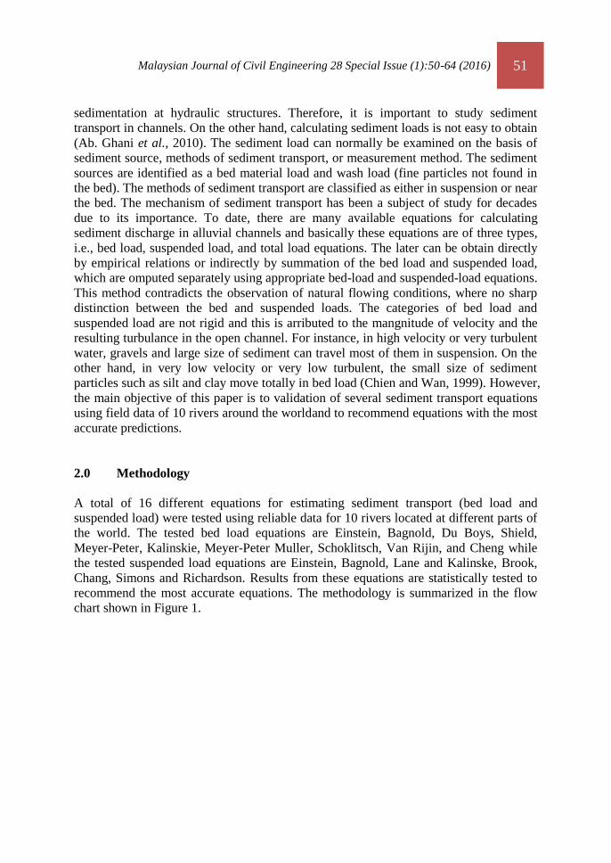
recommend the most accurate equations. The methodology is summarized in the flow

chart shown in Figure 1.

52 Malaysian Journal of Civil Engineering 28 Special Issue (1):50-64 (2016)

Figure 1: Flowchart represents the methodology

2.1 Sediment Field Data

Sediment field data of 10 rivers around the world are selected from published literatures

(Brownlie, 1981). Due to the recommendations made on their reliability, the filed data

have been used for testing the accuracy of the selected sediment transport equations.

Table 1 shows the summery of these data. The following are names of the rivers from

which the field data are collected.

1- Indian canal Data of Chaudry et al. (1970).

2- Colorado River Data of the U.S. Bureau of Reclamation (1958).

3- Middle Loup River Data of Hubbell and Matejka (1959).

4- Mississippi River Data of Toffaleti (1968).

5- Niobrara River Data of the Colby and Hembree (1955).

6- Oak Creek Data of Milhous (1973).

7- Portugal River Data of Da Cunha (1969).

8- Rio Grande Conveyance Channel Data of Culbertson et al. (1976).

9- Snake and Clearwater River Data of Seitz (1976).

10- Trinity River Data of Knott (1974).


Table 1: Summary of field data

No River name Range of

median particle

diameter ( mm)

Range of

discharge

( m3/s)

Range of river

width (m)

Range of

velocity (m/s )

1 Indian canal Data 0.09 – 0.19 109.6 – 424 55.474 -118.262 0.363 - 1.259

2 Colorado 0.236 – 0.36 83.34 – 500.16 92 – 254.55 0.363 – 1.259

3 Middle Loup 0.275-0.395 9.373-11.723 42.977-46.33 0.638-0.94

4 Mississippi 0.165-0.342 22851-28826 1097.3-1109.5 1.344-1.609

5 Niobrara 0.218-0.351 6.456-16.055 21.164-21.946 0.688-1.271

6 Oak Creek 8.2-26 1.416-3.397 5.37-5.914 0.807-1.118

7 Portugal 2.603 59.598-194.094 102-183 0.785-0.973

8 Rio Grande 0.18-0.28 15.857-39.077 20.422-22.86 0.805-1.518

9 Snake and Clearwater 0.52-33 1832-3511.2 176.784-198.12 2.377-2.997

10 Trinity 3.4-11.8 39.642-82.683 30.175-53.95 1.265-2.177

2.2 Bed Load Equations

There are many available equations for estimating bed load in channels and these

equations where based on different concepts. In this study, only 10 of these equations

were applied to estimate the bed load using field data. Table 2 shows these equations.

Table 2: The selected bed load equations

Equation name Concept Equation

Einstein, 1950 Probabilistic defined as the rate of erosions equals the

rate of depositions 𝑞𝑏,𝑤 = 𝜙 ∗ 𝛾𝑠√

𝐷503 ∗ 𝑔(𝜌𝑠 − 𝜌)

𝜌

Eq.(1)

Bagnold, 1966 power concept, its

production of the available stream power and efficiency

𝑞𝑏,𝑤 =𝑃

𝐵

𝑒𝑏

tan 𝛼[

𝛾

𝛾𝑠− 𝛾 ]

Eq.(2)

Du Boys, 1879 and

Straub, 1935

shear stress approach 𝑞𝑏 = 𝑘3 𝜏 ( 𝜏− 𝜏𝑐 ) Eq.(3)

Shield, 1936 shear stress approach 𝑞𝑏𝑣 =

10 𝑞 𝑆0 𝜌2( 𝜏− 𝜏𝑐 )

𝜌𝑠 (𝜌𝑠− 𝜌)2𝑔 𝐷50

Eq.(4)

Meyer – Peter, 1934 energy slope approach 0.4 𝑞𝑏𝑤2/3

𝐷50

= 𝑞𝑤

2/3 𝑆

𝐷50

− 17 Eq.(5)

Kalinske, 1947 shear stress approach 𝑞𝑏𝑣

𝑈∗𝐷= 𝑓 [

𝜏𝑐

𝜏0

] Eq.(6)

Meyer – Peter Muller,

1948

energy slope approach 𝛾 [

𝑘

𝑘′]

3

2

𝑅𝑆 = 0.047 (𝛾𝑠 − 𝛾 )𝐷50 +

0.25 [𝛾

𝑔]

1

3

[𝛾𝑠− 𝛾

𝛾]

2/3

𝑞𝑏𝑤2/3

Eq.(7)

Schoklitsch, 1950 discharge approach 𝑞𝑏𝑤=2500 𝑆3/2 ( 𝑞 − 𝑞𝑐) Eq.(8)

Van Rijin, 2007, a analytical relationship 𝑞𝑏𝑤 = 0.015 𝜌𝑠 𝑉 𝑑 (

𝐷50

ℎ) 1.2𝑀𝑒

1.5 Eq.(9)

Cheng, 2002 An exponential equation is

not including the concept of

critical shear stress

𝑞𝑏𝑤 = [Φ ∗ 𝐷50√𝐷50 ∗ 𝑔 ∗ (𝑠 − 1)] ∗ 𝜌𝑠 Eq.(10)


2.3 Suspended Load Equations

There are many available equations for estimating suspended load in channels and only

six of them were applied to estimate the suspended load using field data. Table 3 shows

these equations.

Table 3: The selected suspended load equations

Equation name Concept Equation

Einstein, 1950 The concepts of these

equations are based on the

exchange theory under

equilibrium conditions and

velocity distribution with some other consumptions

qs,w = 11.6 u∗caa[Ρe I1 + I2]

Eq.(11)

Bagnold, 1966 𝑞𝑠,𝑤=𝑒𝑠(1 − 𝑒𝑏)

𝑃

𝐵

𝑉

𝜔[

𝛾

𝛾𝑠− 𝛾 ]

Eq.(12)

Lane and Kalinske, 1941 qs,w = q CaPL e15ωa/dU∗

Eq.(13)

Brook, 1963 qsw

q Cmd

= TB (k V

U∗ , Z1)

Eq.(14)

Chang, Simons and

Richardson, 1965 qs,w = d Ca (VI1 −2 U∗

kI2 )

Eq.(15)

Van Rijin, 2007, b

analytical relationship qsw = 0.008 ρs V D50Me

2.4(D∗)−0.6 Eq.(16)

2.4 Validation and Statistical Method

Two methods are used to compare the performance of the tested equations and these

methods are Mean Absolute Error (MAE), and Root Mean Square Error (RMSE). The

methods are described by the following equations:

MAE = 1

NΣN=1

N |Qsm − Qsc| (17)

RMSE =√1

𝑁Σ𝑁=1

𝑁 (𝑄𝑠𝑚 − 𝑄𝑠𝑐)2 (18)

where, N is the number of data sets, Qsm is the measured suspended load and Qsc is the

calculated suspended load.

3.0 Results and Discussion

3.1 Comparisons of Bed Load Equations

Hydraulic, sediment and morpholocal data for 10 rivers around the world were used to

estimate the bed loads at different sections (92 sections). The Equations used in

estimating the bedload are (1), (2), (3), (4), (5), (6), (7), (8), (9), and (10). Samples of


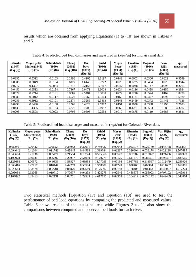
results which are obtained from applying Equations (1) to (10) are shown in Tables 4

and 5.

Table 4: Predicted bed load discharges and measured in (kg/s/m) for Indian canal data

Table 5: Predicted bed load discharges and measured in (kg/s/m) for Colorado River data.

Two statistical methods [Equation (17) and Equation (18)] are used to test the

performance of bed load equations by comparing the predicted and measured values.

Table 6 shows results of the statistical test while Figures 2 to 11 also show the

comparisons between computed and observed bed loads for each river.

Kalinske

(1947)

(Eq.(6))

Meyer peter

Muller(1948)

(Eq.(7))

Schoklitsch

(1950)

(Eq.(8))

Cheng

(2002)

(Eq.(10))

Du

boys

(1879)

(Eq.(3))

Shield

(1936)

(Eq.(4))

Meyer

Peter

(1934)

(Eq.(5))

Einstein

(1950)

(Eq.(1))

Bagnold

(1966)

(Eq.(2))

Van

Rijin

(2007)

(Eq.(9))

qbw

measured

0.0235 0.5312 0.0103 0.2496 0.4165 2.8197 0.0149 0.0602 0.0306 0.0621 0.3549

0.0386 0.3049 0.0154 0.6127 1.6443 6.9272 0.0225 0.0235 0.0434 0.0229 0.3944

0.0217 0.1307 0.0034 0.1717 0.2155 0.9167 0.0042 0.0038 0.0147 0.0095 0.2763

0.0452 0.2512 0.0154 0.7367 2.0478 6.9024 0.0224 0.0136 0.0458 0.0159 0.2924

0.0524 0.2714 0.0191 0.8907 2.5481 8.5830 0.0277 0.0216 0.0524 0.0167 1.0230

0.0385 0.5012 0.0117 0.4023 0.7969 4.3104 0.0165 0.1171 0.0427 0.0597 1.6920

0.0259 0.8912 0.0101 0.2274 0.3289 2.5463 0.0141 0.2469 0.0372 0.1442 1.7126

0.0293 0.8438 0.0108 0.2569 0.4029 2.6397 0.0151 0.2090 0.0388 0.1299 2.2083

0.0436 1.1335 0.0183 0.4226 0.7705 5.1997 0.0262 0.4281 0.0583 0.1680 4.3707

0.0208 0.2598 0.0022 0.0708 0.0396 0.2558 0.0019 0.0675 0.0119 0.0386 0.2841

Kalinske

(1947)

(Eq.(6))

Meyer peter

Muller(1948)

(Eq.(7))

Schoklitsch

(1950)

(Eq.(8))

Cheng

(2002)

(Eq.(10))

Du

boys

(1879)

(Eq.(3))

Shield

(1936)

(Eq.(4))

Meyer

Peter

(1934)

(Eq.(5))

Einstein

(1950)

(Eq.(1))

Bagnold

(1966)

(Eq.(2))

Van Rijin

(2007)

(Eq.(9))

qbw

measured

0.06392 0.20432 0.00652 0.33082 0.32001 0.780332 0.00642 0.023078 0.022739 0.0148778 0.05157

0.094042 0.41004 0.011749 0.45445 0.44598 1.319644 0.01297 0.320904 0.036178 0.0421138 1.507685

0.048684 0.21936 0.005474 0.21564 0.18774 0.505366 0.00547 0.002087 0.018022 0.0174406 0.404973

0.105978 0.80631 0.036392 1.20987 2.54099 9.170279 0.05175 0.611373 0.087401 0.0797487 0.489615

0.125688 1.00372 0.049336 1.58527 3.69958 13.77095 0.07136 0.917789 0.113567 0.1012479 1.253026

0.063416 0.27717 0.010147 0.42769 0.58504 1.558988 0.01249 0.020466 0.02974 0.0211607 0.168085

0.029663 0.33578 0.002701 0.06876 0.02569 0.176902 0.00158 0.128406 0.01313 0.0542097 1.217224

0.095084 0.63065 0.019712 0.70677 0.94233 3.425278 0.02546 0.488876 0.058003 0.0707102 0.403968

0.107892 0.35413 0.022131 1.03751 1.79533 4.617155 0.02958 0.104217 0.056142 0.0242489 0.643064


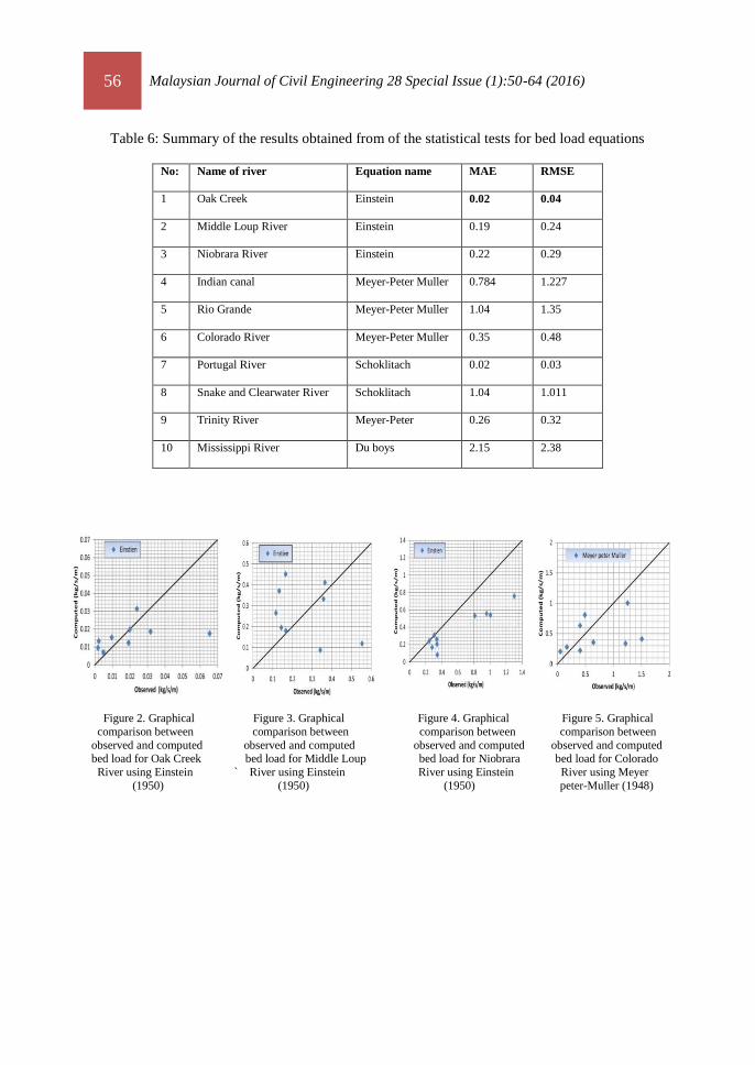
Table 6: Summary of the results obtained from of the statistical tests for bed load equations

No: Name of river Equation name MAE RMSE

1 Oak Creek Einstein 0.02 0.04

2 Middle Loup River Einstein 0.19 0.24

3 Niobrara River Einstein 0.22 0.29

4 Indian canal Meyer-Peter Muller 0.784 1.227

5 Rio Grande Meyer-Peter Muller 1.04 1.35

6 Colorado River Meyer-Peter Muller 0.35 0.48

7 Portugal River Schoklitach 0.02 0.03

8 Snake and Clearwater River Schoklitach 1.04 1.011

9 Trinity River Meyer-Peter 0.26 0.32

10 Mississippi River Du boys 2.15 2.38

Figure 2. Graphical Figure 3. Graphical Figure 4. Graphical Figure 5. Graphical comparison between comparison between comparison between comparison between observed and computed observed and computed observed and computed observed and computed

bed load for Oak Creek bed load for Middle Loup bed load for Niobrara bed load for Colorado

River using Einstein ` River using Einstein River using Einstein River using Meyer

(1950) (1950) (1950) peter-Muller (1948)


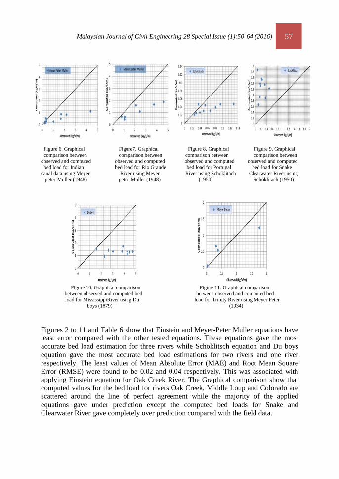
Figure 6. Graphical Figure7. Graphical Figure 8. Graphical Figure 9. Graphical comparison between comparison between comparison between comparison between observed and computed observed and computed observed and computed observed and computed bed load for Indian bed load for Rio Grande bed load for Portugal bed load for Snake canal data using Meyer River using Meyer River using Schoklitach Clearwater River using peter-Muller (1948) peter-Muller (1948) (1950) Schoklitach (1950)

Figure 10. Graphical comparison Figure 11: Graphical comparison

between observed and computed bed between observed and computed bed load for MississippiRiver using Du load for Trinity River using Meyer Peter boys (1879) (1934)

Figures 2 to 11 and Table 6 show that Einstein and Meyer-Peter Muller equations have

least error compared with the other tested equations. These equations gave the most

accurate bed load estimation for three rivers while Schoklitsch equation and Du boys

equation gave the most accurate bed load estimations for two rivers and one river

respectively. The least values of Mean Absolute Error (MAE) and Root Mean Square

Error (RMSE) were found to be 0.02 and 0.04 respectively. This was associated with

applying Einstein equation for Oak Creek River. The Graphical comparison show that

computed values for the bed load for rivers Oak Creek, Middle Loup and Colorado are

scattered around the line of perfect agreement while the majority of the applied

equations gave under prediction except the computed bed loads for Snake and

Clearwater River gave completely over prediction compared with the field data.

Figure 6:Graphical

comparison between

observed and computed bed load for Indian canal

data using Meyer peter-

Muller (1948)

Figure 7: Graphical comparison between

observed and computed

bed load for Rio Grande River using Meyer

peter-Muller (1948)


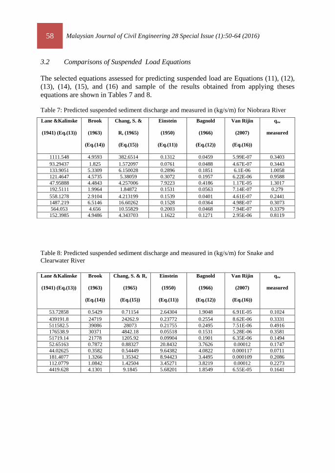
3.2 Comparisons of Suspended Load Equations

The selected equations assessed for predicting suspended load are Equations (11), (12),

(13), (14), (15), and (16) and sample of the results obtained from applying theses

equations are shown in Tables 7 and 8.

Table 7: Predicted suspended sediment discharge and measured in (kg/s/m) for Niobrara River

Table 8: Predicted suspended sediment discharge and measured in (kg/s/m) for Snake and

Clearwater River

Lane &Kalinske

(1941) (Eq.(13))

Brook

(1963)

(Eq.(14))

Chang, S. &

R, (1965)

(Eq.(15))

Einstein

(1950)

(Eq.(11))

Bagnold

(1966)

(Eq.(12))

Van Rijin

(2007)

(Eq.(16))

qsw

measured

1111.548 4.9593 382.6514 0.1312 0.0459 5.99E-07 0.3403

93.29437 1.825 1.572097 0.0761 0.0488 4.67E-07 0.3443

133.9051 5.3309 6.150028 0.2896 0.1851 6.1E-06 1.0058

121.4647 4.5735 5.38059 0.3072 0.1957 6.22E-06 0.9588

47.95888 4.4843 4.257006 7.9223 0.4186 1.17E-05 1.3017

192.5111 1.9964 1.84872 0.1531 0.0563 7.14E-07 0.279

558.1278 2.9104 4.213199 0.1539 0.0401 4.61E-07 0.2441

1487.219 6.5146 16.60262 0.1528 0.0364 4.98E-07 0.3073

564.053 4.656 10.55829 0.2003 0.0468 7.94E-07 0.3379

152.3985 4.9486 4.343703 1.1622 0.1271 2.95E-06 0.8119

Lane &Kalinske

(1941) (Eq.(13))

Brook

(1963)

(Eq.(14))

Chang, S. & R,

(1965)

(Eq.(15))

Einstein

(1950)

(Eq.(11))

Bagnold

(1966)

(Eq.(12))

Van Rijin

(2007)

(Eq.(16))

qsw

measured

53.72858 0.5429 0.71154 2.64304 1.9048 6.91E-05 0.1024

439191.8 24719 24262.9 0.23772 0.2554 8.62E-06 0.3331

511582.5 39086 28073 0.21755 0.2495 7.51E-06 0.4916

176538.9 30371 4842.18 0.05518 0.1531 5.28E-06 0.3581

51719.14 21778 1205.92 0.09904 0.1901 6.35E-06 0.1494

52.65163 0.7872 0.88327 20.8432 3.7626 0.00012 0.1747

44.02625 0.3582 0.54449 9.64382 4.0822 0.000117 0.0711

181.4077 1.3266 1.35342 8.94423 3.4495 0.000109 0.2086

112.0779 1.0842 1.42504 3.45271 3.8219 0.00012 0.2273

4419.628 4.1301 9.1845 5.68201 1.8549 6.55E-05 0.1641


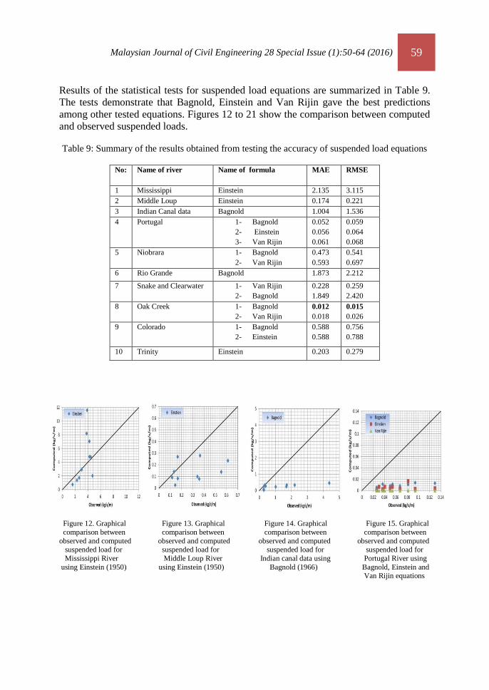
Results of the statistical tests for suspended load equations are summarized in Table 9.

The tests demonstrate that Bagnold, Einstein and Van Rijin gave the best predictions

among other tested equations. Figures 12 to 21 show the comparison between computed

and observed suspended loads.

Table 9: Summary of the results obtained from testing the accuracy of suspended load equations

No: Name of river Name of formula MAE RMSE

1 Mississippi Einstein 2.135 3.115

2 Middle Loup Einstein 0.174 0.221

3 Indian Canal data Bagnold 1.004 1.536

4 Portugal 1- Bagnold

2- Einstein

3- Van Rijin

0.052

0.056

0.061

0.059

0.064

0.068

5 Niobrara 1- Bagnold

2- Van Rijin

0.473

0.593

0.541

0.697

6 Rio Grande Bagnold 1.873 2.212

7 Snake and Clearwater 1- Van Rijin

2- Bagnold

0.228

1.849

0.259

2.420

8 Oak Creek

1- Bagnold

2- Van Rijin

0.012

0.018

0.015

0.026

9 Colorado 1- Bagnold

2- Einstein

0.588

0.588

0.756

0.788

10 Trinity Einstein 0.203 0.279

Figure 12. Graphical Figure 13. Graphical Figure 14. Graphical Figure 15. Graphical comparison between comparison between comparison between comparison between observed and computed observed and computed observed and computed observed and computed suspended load for suspended load for suspended load for suspended load for

Mississippi River Middle Loup River Indian canal data using Portugal River using using Einstein (1950) using Einstein (1950) Bagnold (1966) Bagnold, Einstein and Van Rijin equations


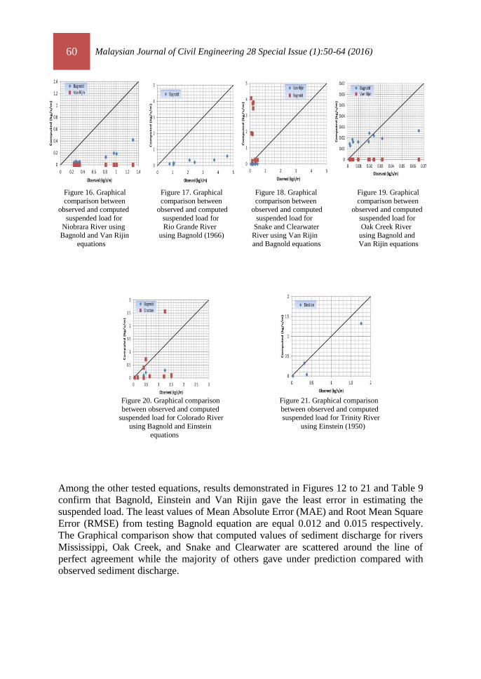
Figure 16. Graphical Figure 17. Graphical Figure 18. Graphical Figure 19. Graphical comparison between comparison between comparison between comparison between observed and computed observed and computed observed and computed observed and computed suspended load for suspended load for suspended load for suspended load for Niobrara River using Rio Grande River Snake and Clearwater Oak Creek River Bagnold and Van Rijin using Bagnold (1966) River using Van Rijin using Bagnold and

equations and Bagnold equations Van Rijin equations

Figure 20. Graphical comparison Figure 21. Graphical comparison between observed and computed between observed and computed suspended load for Colorado River suspended load for Trinity River using Bagnold and Einstein using Einstein (1950)

equations

Among the other tested equations, results demonstrated in Figures 12 to 21 and Table 9

confirm that Bagnold, Einstein and Van Rijin gave the least error in estimating the

suspended load. The least values of Mean Absolute Error (MAE) and Root Mean Square

Error (RMSE) from testing Bagnold equation are equal 0.012 and 0.015 respectively.

The Graphical comparison show that computed values of sediment discharge for rivers

Mississippi, Oak Creek, and Snake and Clearwater are scattered around the line of

perfect agreement while the majority of others gave under prediction compared with

observed sediment discharge.


4.0 Conclusions

The accuracy of selected sediment transport equations have been tested using field data

of 10 rivers around the world and the data describe the sediment, hydraulic and

morphological characteristics of these rivers. Equations found with the most accurate

sediment transport estimation are highlighted. For bed load estimation, validation shows

that Einstein and Meyer-Peter Muller equations have least error compared with

estimation obtained from other tested equations. These equations gave the best bed load

estimation for three rivers while Schoklitsch equation and Du boys equation gave best

bed load prediction for two rivers and one river respectively. The least values of Mean

Absolute Error (MAE) and Root Mean Square Error (RMSE) from testing Einstein

equation using field data of Oak Creek River were found to be 0.02 and 0.04

respectively. For estimation of suspended load, Bagnold, Einstein and Van Rijin gave

the least error compared with the results obtained from applying other tested equations.

The least values of Mean Absolute Error (MAE) and Root Mean Square Error (RMSE)

obtained from testing Bagnold equation are found to be 0.012 and 0.015 respectively.

Validation of the selected sediment transport equations show that there is no unique

equation that can always give accurate prediction for all rivers. This is can be attributed

to the fact that different rivers has different hydraulic and morphological characteristics

such as discharge, velocity, energy slope, bed forms, median diameter, and sinuosity.

Notations

qb,w = Bed load transport (Kg/s /m)

ϕ = Einstein bed load function

s = slope

ν = viscosity of the fluid

ρs= sediment density (kg /m3)

γs = specific gravity of sediment (ρs ∗ g )

ρ = fluid density (kg /m3)

g = gravity acceleration (m/s2)

D50 = particle diameter (m)

P

B= τ V = ρ g R s V

V = mean velocity m/s


eb= efficiency factor of bed load

tan α = coefficient obtained

k3 = 0.173

Ds3/4 , qb,v = bed load transport rate (m

3/s/m)

q=discharge per unit width (m3/s/m)

qw= discharge in unit of (kg/s/m)

Τc = 0.12 (γs − γ )D

k =Strickler roughness equation=1/n = V

R23 S

12

,

k′= roughness coefficient due to the bedforms = 26

D901/6

qc = 0.26 [γs− γ

γ]

5/3 D3/2

S7/6in unit (m3/s /m)

Me= mobility parameter = (V−ucr)

[(S−1)gD50]0.5

d= water depth

ucr = critical velocity

ucr = 0.19(D50)0.1 log [12 d

3 D90]for 0.0001<D90< 0.0005 m

ucr = 8.5(D50)0.6 log [12 d

3 D90]for 0.0005<D90< 0.002 m

Φ = 13 ∗ Ω ∗ EXP [−0.05

Ω]

Ω = τ ∗ U∗

ρ [(S−1)gD50]32

qs,w = Suspended load transport (kg/s/m)

Ca= reference concentration (volume) = 1

11.6

qb,w

u∗ a

a = reference level=2D65

Ρe = 2.303 log30.2 d

Δ

A=a/h dimensionless reference level


Z=ws/(ku∗) suspension number, the I1 and I2 integrals can be determined graphically relate to

the A and Z

ω = fall velocity of sediment (m/s)

es= efficiency factor of suspended load

Ca = concentration by weight at y = a

PL = factor in a function of ω

U∗ and n

d16

Cmd = reference sediment concentration at d/2 where d is the depth of flow

k = Von Karman constant = 0.4, Z1 =Z

β, Z=

ω

k U∗

I1and I2 determined from the graph in term of ξa and Z2

ξa =a

d

Z2 =2 ω

β U∗ k , D∗ =dimensionless particle size.

References

Ab. Ghani, A., Azamathulla, H. Md., Chang, C. K., Zakaria, N. A., Abu Hasan, Z. (2010).

Prediction of total bed material load for rivers in Malaysia: A case study of Langat, Muda

and Kurau Rivers. Environ Fluid Mech (2011) 11:307–318.

Brooks, N.H. (1963). Calculation of suspended load discharge from velocity and concentration

parameters.Proceedings of Federal Interagency Sedimentation Conference, U.S. Department

of Agriculture, Miscellaneous Publication no. 970.

Bagnold, R. A. (1966). An Approach to the Sediment Transport Problem from General Physics.

U.S. Geological Survey Professional Paper 422-J.

Brownlie, W. R. (1981). Compilation of alluvial channel data: Laboratory and Field. Rep. No.

KH-R-43B, California Institute of Technology, Calif.

Chang, F. M., D. B. Simons, and E. V. Richardson (1965). Total Bed-Material Discharge in

Alluvial Channels. U.S Geological Survey Water-Supply Paper 1498-I.

Cheng, N. S. (2002). Exponential Formula for Bedload Transport. Journal of Hydraulic

Engineering, vol. 128, no. 10.

Chien, N., and Wan, Z. (1999). Mechanics of Sediment Transport. ASCE, Reston, Va.

DuBoys, M. P. (1879). Le Rhone et les Rivieres a Lit affouillable. Annales de Ponts et Chausses,

sec. 5, vol. 18, pp. 141-195.

Einstein, H. A. (1950). The Bed Load Function for Sediment Transportation in Open Channel

Flows. U.S. Department of Agriculture, Soil Conservation Service, Technical Bulletin no.

1026.

Graf, Walter Hans (1971): Hydraulics of sediment transport. McGraw-Hill, Inc.


Lane, E. W., and A. A. Kalinske (1941). Engineering Calculations of Suspended Sediment.

Transactions of the American Geophysical Union, vol. 20, pt. 3, pp. 603-607.

Meyer-Peter, E., and R. Müller (1948). Formulas for bed load transport. Report on second

meeting of international association for Hydraulics Research, Stockholm, Sweden, pp. 39-64

Meyer-Peter, E., H. Favre, and Einstein, A. (1934). Neuere Versuchsresultate über den

Geschiebetrieb. Schweiz Bauzeitung, vol. 103, no.13.

Schoklitsch, A. (1950) Handbuch des Wasserbaues, [Handbook of Hydraulic Structures] 2nd

edn, Vienna, Austria: Springer.

Shields, A. (1936). Anwendung der Aenlichkeitsmechanik und Turbulenz forschung auf die

Geschiebebewegung. Mitteil. Preuss. Versuchsanst. Wasser, Erd, Schiffsbau, Berlin, Nr. 26.

Straub, L. G., (1935). Missouri River Report. In-House Document 238, 73rd Congress, 2nd

Session, U.S Government Printing Office, Washington, D.C., p. 1135.

Van Rijn, L. C. (2007, a). Unified view of sediment transport by currents and waves, I: Initiation

of motion, bed roughness, and bed-load transport. Journal of Hydraulic Engineering, 133(6),

p 649-667.

Van Rijn, L. C. (2007, b). Unified view of sediment transport by currents and waves, II:

Suspended transport. Journal of Hydraulic Engineering, 133(6), p 668-389.

Van Rijn, L. C. (1993). Principle of Sediment Transport in Rivers, Estuaries and Coastal Seas.

Aqua Publications, Amsterdam multiple pagination.

Yang, S. Q. (2010). Sediment Transport Capacity in Rivers. Journal of Hydraulic Research, vol.

42, no. 3(2005), pp. 131-138.

Documents

Hydar L. Ali*, Thamer Ahamed Mohammed, …...Hydar L. Ali*, Thamer Ahamed Mohammed, Badronnisa Yusuf & Azlan A. Aziz Department of Civil Engineering, Faculty of Engineering, Universiti

Hydar L. Ali, Thamer Ahamed Mohammed, …...Hydar L. Ali, Thamer Ahamed Mohammed, Badronnisa Yusuf & Azlan A. Aziz Department of Civil Engineering, Faculty of Engineering, Universiti