Embed Size (px)
Citation preview
Hydration, Ion Binding and
Self-Aggregation of Choline and
Choline-based Surfactants
Dissertationzur Erlangung des
Doktorgrades der Naturwissenschaften(Dr. rer. nat.)
der Naturwissenschaftlichen Fakultät IVChemie und Pharmazie
der Universität Regensburg
vorgelegt vonSaadia Shaukat
aus Rawalpindi / Pakistan
Regensburg 2012
Promotionsgesuch eingereicht am: 30.10.2012
Tag des Kolloquiums: 20.12.2012
Die Arbeit wurde angeleitet von: Apl. Prof. Dr. R.Buchner
Prüfungsausschuss: Apl. Prof. Dr. R.BuchnerProf. Dr. W.KunzProf. Dr. A. PtznerProf. Dr. D. Horinek (Vorsitzender)
Dedicated to
My Parents, Abd Ur Rahman, Huzaifa
and
Hamza

Contents
Introduction 1
1 Theoretical background 5
1.1 Fundamental equations of electromagnetism . . . . . . . . . . . . . . . . . 51.1.1 Maxwell equations . . . . . . . . . . . . . . . . . . . . . . . . . . . 51.1.2 Constitutive equations for static or low elds . . . . . . . . . . . . 61.1.3 Equations for dynamic eld . . . . . . . . . . . . . . . . . . . . . . 61.1.4 Reduced wave equations for electric and magnetic elds . . . . . . . 8
1.2 Dielectric relaxation . . . . . . . . . . . . . . . . . . . . . . . . . . . . . . 91.2.1 Polarization response . . . . . . . . . . . . . . . . . . . . . . . . . . 91.2.2 Response functions of the orientational polarization . . . . . . . . . 10
1.3 Empirical description of dielectric relaxation . . . . . . . . . . . . . . . . . 111.3.1 Debye equation . . . . . . . . . . . . . . . . . . . . . . . . . . . . . 121.3.2 Non-Debye type relaxations . . . . . . . . . . . . . . . . . . . . . . 121.3.3 Damped harmonic oscillator . . . . . . . . . . . . . . . . . . . . . . 131.3.4 Combination of models . . . . . . . . . . . . . . . . . . . . . . . . . 14
1.4 Microscopic models of dielectric relaxation . . . . . . . . . . . . . . . . . . 141.4.1 Onsager equation . . . . . . . . . . . . . . . . . . . . . . . . . . . . 141.4.2 Kirkwood-Fröhlich equation . . . . . . . . . . . . . . . . . . . . . . 151.4.3 Cavell equation . . . . . . . . . . . . . . . . . . . . . . . . . . . . . 161.4.4 Microscopic and macroscopic relaxation times . . . . . . . . . . . . 161.4.5 Debye model of rotational diusion . . . . . . . . . . . . . . . . . . 171.4.6 Molecular jump model . . . . . . . . . . . . . . . . . . . . . . . . . 18
1.5 Temperature dependence of relaxation times . . . . . . . . . . . . . . . . . 191.5.1 Arrhenius equation . . . . . . . . . . . . . . . . . . . . . . . . . . . 191.5.2 Eyring equation . . . . . . . . . . . . . . . . . . . . . . . . . . . . . 20
1.6 Solute-related relaxations . . . . . . . . . . . . . . . . . . . . . . . . . . . . 201.6.1 Ion-pair relaxation . . . . . . . . . . . . . . . . . . . . . . . . . . . 201.6.2 Ion-cloud relaxation . . . . . . . . . . . . . . . . . . . . . . . . . . 221.6.3 Grosse's model . . . . . . . . . . . . . . . . . . . . . . . . . . . . . 23
i
ii CONTENTS
2 Experimental 252.1 Sample preparation . . . . . . . . . . . . . . . . . . . . . . . . . . . . . . . 252.2 Measurement of dielectric properties . . . . . . . . . . . . . . . . . . . . . 26
2.2.1 Time-domain reectometry . . . . . . . . . . . . . . . . . . . . . . . 262.2.2 Interferometry . . . . . . . . . . . . . . . . . . . . . . . . . . . . . . 292.2.3 Vector network analysis . . . . . . . . . . . . . . . . . . . . . . . . 332.2.4 Data analysis . . . . . . . . . . . . . . . . . . . . . . . . . . . . . . 38
2.3 Auxiliary measurements . . . . . . . . . . . . . . . . . . . . . . . . . . . . 402.3.1 Densimetry . . . . . . . . . . . . . . . . . . . . . . . . . . . . . . . 402.3.2 Conductivity . . . . . . . . . . . . . . . . . . . . . . . . . . . . . . 402.3.3 Viscometry . . . . . . . . . . . . . . . . . . . . . . . . . . . . . . . 412.3.4 MOPAC calculations . . . . . . . . . . . . . . . . . . . . . . . . . . 41
3 Investigation of electrolyte solutions 433.1 Physical properties of choline chloride, chlorocholine chloride and ammonium chloride 44
3.1.1 Results and discussion . . . . . . . . . . . . . . . . . . . . . . . . . 443.2 DRS of choline chloride, chlorocholine chloride and ammonium chloride . . 61
3.2.1 Choice of t model . . . . . . . . . . . . . . . . . . . . . . . . . . . 613.2.2 Resolution of DR spectra and assignment of relaxation modes. . . 653.2.3 Solute dispersion. . . . . . . . . . . . . . . . . . . . . . . . . . . . 683.2.4 Solvent dispersion. . . . . . . . . . . . . . . . . . . . . . . . . . . 723.2.5 Ion hydration. . . . . . . . . . . . . . . . . . . . . . . . . . . . . . 753.2.6 Temperature dependence of bulk water dynamics. . . . . . . . . . 77
4 Investigation of micellar systems 814.1 Aqueous solutions of sodium laurate . . . . . . . . . . . . . . . . . . . . . . 83
4.1.1 Resolution of DR spectra . . . . . . . . . . . . . . . . . . . . . . . . 844.1.2 Assignment of micelle-specic modes . . . . . . . . . . . . . . . . . 86
4.2 DRS of bio-compatible surfactants . . . . . . . . . . . . . . . . . . . . . . . 924.2.1 Aqueous solutions of choline laurate . . . . . . . . . . . . . . . . . . 924.2.2 Resolution of DR spectra . . . . . . . . . . . . . . . . . . . . . . . . 934.2.3 Assignment of micelle-specic modes . . . . . . . . . . . . . . . . . 954.2.4 Aqueous solutions of choline dodecylsulfate . . . . . . . . . . . . . . 1004.2.5 Resolution of DR spectra . . . . . . . . . . . . . . . . . . . . . . . . 1004.2.6 Assignment of micelle-specic modes . . . . . . . . . . . . . . . . . 1014.2.7 Solvent relaxations and micellar hydration . . . . . . . . . . . . . . 1074.2.8 Eect of added salt on dielectric properties of choline dodecylsulfate 112
Summary and conclusions 117
Bibliography 120

Preface
This dissertation is based on research carried out between February 2009 and October 2012at Institute of Physical and Theoretical Chemistry (Faculty of Natural Sciences IV) of theUniversity of Regensburg.
I would like to express my sincere thanks to my supervisor Prof. Dr. Richard Buchnerfor providing me the opportunity to work in his group. His continuous guidance andencouragement throughout the whole period of my PhD studies helped me to successfullycomplete the designed project work.
I would like to express my gratitude to the head of the institute Prof. Dr. Werner Kunz forproviding the laboratory facilities. Furthermore, his support in terms of providing requiredannual referee's report is highly acknowledged.
I am also thankful to the Higher Education Commission of Pakistan (HEC) for a PhDgrant and German Academic Exchange Service (DAAD) for guidance and support.
I would like to express my gratitude to my current and former colleagues in the microwavegroup, Dr. Johannes Hunger, Dr. Alexander Stoppa, Dr. Haz Muhammad Abd Ur Rah-man, Thomas Sonnleitner, Andreas Eiberweiser, and Bernd Muehldorf, for their supportand valuable discussions.
Thanks to all members of workshops for completing my orders reliably and quickly. Fur-thermore, I would like to thank all sta members of the Institute of Physical and TheoreticalChemistry for their cooperativeness.
Finally, I wish to express my profound gratitude to my beloved parents, husband andbrothers for their love and continuous support.

Constants, symbols and acronyms
Constants
elementary charge e0 = 1.60217739 · 10−19 C
permittivity of free space ε0 = 8.854187816 · 10−12 C2(Jm)−1
Avogadro's constant NA = 6.0221367 · 1023 mol−1
speed of light c0 = 2.99792458 · 108ms−1
Boltzmann's constant kB = 1.380658 · 10−23 JK−1
permeability of free space µ0 = 4π · 10−7 (Js)2(C2m)−1
Planck's constant h = 6.6260755 · 10−34 Js
Symbols
B magnetic induction [Vsm−2] D electric induction [Cm−2]
E electric eld strength [Vm−1] H magnetic eld strength [Am−1]
ν frequency [s−1] ω angular frequency [s−1]
P polarization [Cm−2] µ dipole moment [Cm]
ε complex dielectric permittivity ε′ real part of ε
ε′′ imaginary part of ε ε limν→0(ε′)
ε∞ limν→∞(ε′) τ relaxation time [s]
T thermodynamic temperature [K] c molarity[mol dm−3
]κ conductivity [Sm−1] ρ density [kgm−3]
Acronyms
DRS dielectric relaxation spectroscopy NMR nuclear magnetic resonance
IFM interferometer VNA vector network analyzer
TDR time domain reectometry MD molecular dynamics
DMA N ,N -dimethylacetamide PC propylene carbonate
SED Stokes-Einstein-Debye HN Havriliak-Negami
D Debye CC Cole-Cole
CD Cole-Davidson DHO damped harmonic oscillator

Introduction
Basic aspects
Since long, the study of structure and dynamics of electrolyte solutions has been a topicof profound interest. Several theories and experimental techniques have been evolved tounderstand the behavior of so called simple electrolytes and a vast body of data has beengenerated for these systems. However, the level of agreement between the results obtainedfrom dierent methods/techniques puts a questionmark on our claimed understanding ofthese systems. For electrolyte solutions, in order to grip the knowledge of fundamentalmolecular level mechanisms behind various phenomena, a thorough understanding of ion-association and ion-hydration is necessary. In case of aqueous solutions the co-operativedynamics of hydrogen bonded network of water could be probed to study solute eects onwater in terms of its hydration and/or aggregation pattern. It is known that hydration ofsmall and large particles diers qualitatively, with a crossover on nanometer length scale,1
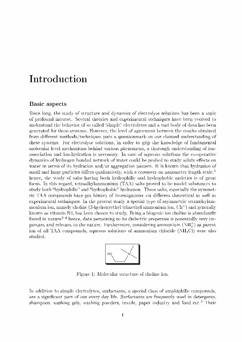
hence, the study of salts having both hydrophilic and hydrophobic moieties is of greatfocus. In this regard, tetraalkylammonium (TAA) salts proved to be model substances tostudy both hydrophilic and hydrophobic hydration. These salts, especially the symmet-ric TAA compounds have got history of investigations via dierent theoretical as well asexperimental techniques. In the present study a special type of asymmetric tetraalkylam-monium ion, namely choline (2-hydroxyethyl trimethyl ammonium ion, Ch+) and generallyknown as vitamin B4, has been chosen to study. Being a biogenic ion choline is abundantlyfound in nature24 hence, data pertaining to its dielectric properties is potentially very im-portant and relevant to the nature. Furthermore, considering ammonium (NH+
4 ) as parention of all TAA compounds, aqueous solutions of ammonium chloride (NH4Cl) were alsostudied.
HO N+
Figure 1: Molecular structure of choline ion.
In addition to simple electrolytes, surfactants, a special class of amphiphilic compounds,are a signicant part of our every day life. Surfactants are frequently used in detergents,shampoos, washing gels, washing powders, textile, paper industry and food etc.5 Their
1
2 INTRODUCTION
presence in such vast variety of elds make them inevitable for us. Most commonly knownsurfactants are soaps, which are used since thousands of years.6 Due to their usage in suchversatile elds, surfactants are synthesized in enormous amounts and thus large concernsabout their eco-friendliness and biodegradability arise. As already mentioned, choline isan ion of biological origin, surfactants having choline as counterions have been successfullysynthesized and patented by the University of Regensburg.7 Details of their cytotoxic andbiodegradability analysis are available in literature.8 Furthermore, room temperature ionicliquids (RTIL) having choline as cations are also a eld of growing interest.8,9 So usingcholine as a bio-relevant ion, opens a horizon to design a wide range of green materials.Present study includes investigations of two types of systems, i.e., choline-based electrolytesand choline-based surfactants. Special emphasis is given on hydration, ion-binding and self-association of these compounds. Aqueous solutions of choline containing compounds havebeen studied through dielectric relaxation spectroscopy (DRS). Principally, DRS probesthe uctuations of permanent dipoles in response to an oscillating electromagnetic eld inthe microwave (GHz) region and is sensitive to reorientational and cooperative motions ofdipolar species in pico- to nanosecond timescale.10 Furthermore, DRS has unique sensitivitytowards dierent types of ion pairs which many other experimental methods lack.10,11
The dissertation includes as well, a set of supplementary measurements for conductivitiesand densities for each of the studied system. Moreover, viscosity data is also reported forfew systems only.
Systems investigated and motivation
The main aim of present study is the application of DRS to aqueous solutions of choline-based electrolytes and surfactants. For this purpose, choline chloride (ChCl), chlorocholinechloride (Cl-ChCl) and ammonium chloride (NH4Cl) have been chosen as examples ofelectrolytes. Comparison is made between the DRS results of tetra-n-alkylammoniumions12 and our ndings for choline salts. Reasonable concentration range have been studiedfor each of these systems. Special features like ion pairing and ion hydration have beenstudied in detail for these solutions.For the investigations of micellar systems two bio-compatible surfactants, namely cholinedodecanoate (ChC12) and choline dodecylsulfate (ChDS), and sodium dodecanoate (NaC12)have been studied. Despite the fact that natural soaps are easy to prepare and are at thesame time ecofriendly, neverthless, long chain derivatives of theses soaps are most desireddue to better detergency and related properties. This however, has to be done at thecost of decreased water solubility. As, for example, under ambient conditions, sodiumand potassium soaps can be prepared upto a maximum chain length of twelve carbons.13
This arose the demand of having such surfactants which have better solubility and at leastsimilar biodegradability as do the natural soaps possess. In this regard surfactants withcholine as counterions (synthesized in the University of Regensburg) are claimed to havepronouncedly lower krat points compared to their corresponding alkali counterparts andare non-toxic and biologically degradable.14 Being new, the literature data pertaining toChC12 and ChDS is scarce, hence, the presented work aimed to investigate dielectricallyaqueous solutions of ChC12 and ChDS. It was also aimed to compare the results of choline-

INTRODUCTION 3
based surfactants with corresponding surfactants having sodium (Na+) as counterion. Forthis purpose literature data of sodium dodeylsulfate (SDS)15 was used and the experi-mental work was extended to study aqueous solutions of NaC12 as well. For the micellarsolutions DRS has proved to be a promising tool to investigate various micelle-related pro-cesses and distinct dynamics of water in bound state (as a part of hydration shell) and infree state (bulk water). Features like micelle-specic relaxations, micellar hydration andcounterion-headgroup binding have been studied in detail. The potential of the presentedwork using DRS should through some light on various micelle-related properties. Based onspecic ion eects16 and Collins's law of matching water anities,17,18 it is expected thatcounterion-headgroup binding is preferable for soft-soft and hard-hard couple compared tosoft-hard binding. This is cross checked for the studied surfactants having two types ofheadgroups, RCO−
2 and ROSO−3 , and counterions, Na+ and Ch+. The hydration pattern
of these surfactants is used to explain dierence in the preferential binding of choline andsodium ions to carboxylate or sulfate headgroups. In order to validate the claimed lowsalt sensitivity of choline dodecylsulfate,8 aqueous solutions of ChDS with added NaCland ChCl are additionally measured and the obtained spectra are analyzed qualitatively.Dielectric spectra have been recorded over a suciently broad frequency range, 0.01 or 0.2≤ ν/GHz ≤ 89.It should be noted that, for the measurements of micellar systems, low frequency data(down to few tens of MHz) was indeed necessary. This however, oered major dicultiesregarding the optimization of proper cells to reduce electrode polarization and related un-wanted features. An empirical methodology is adopted to overcome this undesired featurefrom the DR spectra of micellar solutions, wherever necessary.

Chapter 1
Theoretical background
1.1 Fundamental equations of electromagnetism
1.1.1 Maxwell equations
All electro-magnetic phenomena are governed by the Maxwell's equations19,20 which arebased on four laws as
rot H = j +∂
∂tD (1.1)
rot E = − ∂
∂tB (1.2)
div D = ρel (1.3)
div B = 0 (1.4)
Where H is magnetic and E is electric eld strength, j represents the current density andB and D account for the magnetic and electric induction, also called magnetic ux densityor electric displacement eld, respectively whereas ρel, is electric charge density. Eq. 1.1(Ampère-Maxwell's law) gives a quantitative description of production of magnetic eldsby the electric current. Faraday's law of electro-magnetic induction (Eq. 1.2) describes thegeneration of electric eld if the magnetic ux going across a closed circuit changes. Gauss'slaw of electric eld (Eq. 1.3) states that, on a closed surface, the number of lines of electricux going through that surface equals the total quantity of electric charge contained withinit. Eq. 1.4 (Gauss's law of magnetic eld) is nothing but an expression for the fact thatmagnetic ux does not have origins.The above mentioned laws along with the Newton equation
m∂2
∂t2r = q(E + v × B) (1.5)
are sucient to explain all electro-magnetic phenomena. In the above equation q denotesa moving charge and v is its velocity.
5

6 CHAPTER 1. THEORETICAL BACKGROUND
1.1.2 Constitutive equations for static or low elds
The relation between the dielectric displacement (D) and electric eld strength (E) canbe written as21
D = εε0E (1.6)
which is applicable only for homogenous, non-dispersive, isotropic materials at static (time-independent) and low elds (linear response regime). In the above relation ε is the relativepermittivity and ε0 is the the dielectric permittivity of vacuum. Similarly a linear rela-tionship between H and B can be dened as
H =B
µµ0
(1.7)
where µ is the relative magnetic permittivity and µ0 is the magnetic permittivity of vacuum.The relation between µ0 and ε0 is given by, µ0 = 1/ε0c
2, where c is the velocity of light invacuum.Similar to Eq. 1.6 Ohms law
j = κE (1.8)
gives the relationship between j and E where κ is the electric conductivity.The constitutive equations (Eqs. 1.6 - 1.8), which relate D and H to E and B by time-and eld strength-independent scalars (material properties) like ε, κ and µ, are valid onlyfor the special case of a time-independent eld response.
1.1.3 Equations for dynamic eld
The simplest description of dynamic elds can be done with the help of sinusoidally varying(harmonic) electric elds. The time dependence of electric eld strength is given by21
E(t) = E0 cos(ωt) (1.9)
In the above equation E0 is the amplitude and ω = 2πν the angular frequency of thesinusoidally varying electric eld. When the frequency of the sinusoidal variation is suf-ciently high (typically in the region of 1MHz to 1GHz for the condensed phase), themotion of the microscopic particles does not follow the changes in the eld due to inter-action or inertia within the system, hence both polarization and dielectric displacementcan no longer be described by the quasi-static relations. For a linear and isotropic systema frequency-dependent phase delay, δ(ω), is observed between the electric eld and theelectric displacement as
D(t) = D0 cos(ωt− δ(ω)) (1.10)
where D0 is the amplitude of the sinusoidal variation. Splitting Eq. 1.10 according to theaddition theorem of the cosine function into two sinusoidally varying parts, one in phaseand the other having a phase dierence of π/2 with the electric eld yields
D(t) = D0 cos(δ(ω)) cos(ωt) + D0 sin(δ(ω)) sin(ωt) (1.11)
1.1. FUNDAMENTAL EQUATIONS OF ELECTROMAGNETISM 7
Accordingly a new notation can be introduced as
D0 cos(δ(ω)) = ε′(ω)ε0E0 (1.12)
D0 sin(δ(ω)) = ε′′(ω)ε0E0 (1.13)
so that the electric displacement eld can be expressed as
D(t) = ε′(ω)ε0E0 cos(ωt) + ε′′(ω)ε0E0 sin(ωt) (1.14)
and the phase delay as
tan(δ(ω)) =ε′′(ω)
ε′(ω)(1.15)
In case of static eld (ω = 0), the Eq. 1.14 reduces to:
D(t) = ε′(0)ε0E0 (1.16)
In Eq. 1.14, D(t) has contributions from the frequency dependent relative permittivity(or the frequency dependent dielectric constant), ε′(ω), and the loss factor, ε′′(ω), whichdetermines the loss of energy in the dielectric. By using complex notation, the complex
eld vectors ( ˆE(t) and ˆD(t)) and related constitutive equations can be rewritten for the
dynamic elds as21
ˆE(t) = E0 cos(ωt) + iE0 sin(ωt) = E0 exp(iωt) (1.17)ˆD(t) = D0 cos(ωt− δ) + iD0 sin(ωt− δ) = D0 exp[i(ωt− δ)] (1.18)
and thusε(ω) = ε′(ω)− iε′′(ω) (1.19)
For zero frequency, however the complex dielectric constant changes into the static dielectricconstant, i.e. ε = ε′(0).Hence
ˆD(t) = ε(ω)ε0
ˆE(t) (1.20)
ˆj(t) = κ(ω)
ˆE(t) (1.21)
ˆB(t) = µ(ω)µ0
ˆH(t) (1.22)
Where µ(ω) is the complex relative magnetic permeability and κ(ω) is the complex con-ductivity of the dielectric.
8 CHAPTER 1. THEORETICAL BACKGROUND
1.1.4 Reduced wave equations for electric and magnetic elds
As already mentioned, the harmonic eld can be represented in a compact way by using acomplex notation as
ˆE(t) = E0 exp(iωt) (1.23)ˆH(t) = H0 exp(iωt) (1.24)
Comparison of complex constitutive equations (1.20 - 1.22) with the Maxwell equations(1.1 and 1.2) results in
rot H0 = (κ(ω) + iωε(ω)ε0)E0 (1.25)
and
rot E0 = −iωµ(ω)µ0H0 (1.26)
Subsequent application of the rotation operator to Eq. 1.25 in combination with Eq. 1.26and the Legendre vectorial identity yields
rot rot H0 = grad div H0 −H0 = grad (0)−H0 = − H0 (1.27)
the reduced wave equation of the magnetic eld
H0 + k2H0 = 0 (1.28)
Where k, in the above equation is dened as propagation constant
k2 = k20
(µ(ω)ε(ω) +
µ(ω)κ(ω)
iωε0
)(1.29)
The propagation constant of free space, k0, is given by
k0 = ω√ε0µ0 =
2π
λ0
(1.30)
with
c0 =1
√ε0µ0
(1.31)
where c0 and λ0 are the speed of light and the wavelength of a monochromatic wave invacuum, respectively. For a source-free medium (div E = 0) a reduced wave equation forE can be obtained
ˆE0 + k2 ˆ
E0 = 0 (1.32)

1.2. DIELECTRIC RELAXATION 9
Since for non-magnetizable materials, µ = 1, hence Eq. 1.29 can be written as
k2 = k20
(ε(ω) +
κ(ω)
iωε0
)≡ k2
0 η(ω) (1.33)
and the generalized complex permittivity, η(ω) = η′(ω) − iη′′(ω), is dened with its realand imaginary parts as
η′(ω) = ε′(ω)− κ′′(ω)
ωε0(1.34)
η′′(ω) = ε′′(ω) +κ′(ω)
ωε0(1.35)
Note that η(ω) is the only experimentally accessible quantity in a dielectric experiment.Applying the limits of κ(ω), i.e., limν→0 κ
′ = κ and limν→0 κ′′ = 0, where κ is the dc
conductivity, helps to separate the conductivity contribution from the η(ω) as
ε′(ω) = η′(ω) (1.36)
and
ε′′(ω) = η′′(ω)− κ
ωε0(1.37)
The complex relative permittivity, ε(ω) encapsulates all contributions to the time depen-dent polarization, P (t), that depend on frequency, irrespective of their rotational, vibra-tional, or translational character, hence reects the dynamics of the investigated system.This includes the dispersion of conductivity due to ion-cloud relaxation22 as well.
1.2 Dielectric relaxation
1.2.1 Polarization response
For a non-conducting system the polarization ˆP is related to the dielectric displacement
eld ˆD which originates from the response of a material to an external eld only, hence
ˆP =
ˆD − D0 = εε0
ˆE − ε0
ˆE (1.38)
thus
ˆP = (ε− 1)ε0
ˆE (1.39)
Where χ = (ε− 1), is the dielectric susceptibility of the material under the inuence of an
outer electric eld and ε0ˆE is independent of medium.
The macroscopic polarization ˆP can be related to its microscopic constituents which de-
scribe the microscopic dipole moments of the particles as21,23
ˆP =
ˆPµ +
ˆPα (1.40)
10 CHAPTER 1. THEORETICAL BACKGROUND
where ˆPµ denotes orientational polarization (originating due to presence of permanent
dipoles which are oriented by an electric eld) and ˆPα is induced polarization (could be of
electronic or atomic in nature).
ˆPµ =
∑k
ρk⟨µk⟩ (1.41)
ˆPα =
∑k
ρkαk(ˆEi)k (1.42)
Eq. 1.41 describes the orientation of molecular dipoles of species k with permanent dipolemoment, µk, and number density, ρk, in the external eld against their thermal motion.However, Eq. 1.42 describes the induced polarization for species with molecular polariz-
ability, αk, in the medium caused by the inner eld, ( ˆEi)k, (which distorts the neutraldistribution of charges) acting at the position of the molecule.Orientational polarization in liquids occurs at pico- to nanosecond time scales, correspond-ing to an approximate frequency scale of 1 MHz to 10 THz. Due to the coupling of thereorienting dipoles with the surrounding medium rather broad bands are observed. In thisregard, determination of the frequency dependent complex permittivity can provide valu-able insight into the dynamics of liquids.
The value of ˆPα is rather constant in the microwave range and its frequency dependence
leads to information about the intramolecular dynamics of the system. It consists of twocontributions, one in the infrared (atomic polarization) and the other in the ultravioletrange (electron polarization). The absorption peaks are in most cases sharper comparedto those at microwave frequencies.24
Due to the dierent time scales of ˆPµ and ˆ
Pα, both eects are generally well separated andcan be regarded as linearly independent.25 Thus the induced polarization can be incorpo-rated into the innite frequency permittivity, ε∞, as
ˆPµ = ε0(ε− ε∞)
ˆE (1.43)
ˆPα = ε0(ε∞ − 1)
ˆE (1.44)
Situated in the far-infrared, ε∞ denotes the permittivity after the decay of orientationalpolarization, whereas the contribution arising from induced polarization still remains un-changed. In practice, the limiting value of the permittivity for innite frequencies asextrapolated from the microwave range is taken for ε∞.24
1.2.2 Response functions of the orientational polarization
In the time scale ranging from mega-hertz to the giga-hertz frequencies, ˆPµ lags behind
the changes in the applied eld ˆE as the molecular dipoles cannot align parallel to the

1.3. EMPIRICAL DESCRIPTION OF DIELECTRIC RELAXATION 11
alternating eld due to inertia and friction. On the other hand, the induced polarizationˆPα always remains in equilibrium with the applied eld.In case of an isotropic linear dielectric (linearity holds if a eld E1 generates a polarizationP1 and eld E2 a polarization P2, then the eld E1 + E2 results in a polarization P1 + P2)exposed to a jump in the applied eld strength at t = 0, the time-dependent polarizationˆPµ(t) can be represented by the equilibrium values corresponding to the eld at t ≤ to,ˆPµ(0), and at t > to,
ˆPµ(∞). The corresponding polarization can be written as21
ˆPµ(t) =
ˆPµ(0) · F or
P (t) (1.45)
where F orP (t) is the step response function of the polarization. It is dened as
F orP (t) =
⟨Pµ(0) · Pµ(t)⟩⟨Pµ(0) · Pµ(0)⟩
(1.46)
For t = 0 it follows that F orP (0) = 1; for high values of t, ˆ
P will reach the equilibriumvalue and consequently F or
P (∞) = 0. The time domain reectometry (TDR), one of theexperimental technique used in the presented work, is based on this principle.26
For a monochromatic harmonic electric eld, ˆE(t) =
ˆE0 exp(−iωt) of angular frequency,
ω, the orientational polarization at any time t can be expressed as
ˆP (ω, t) = ε0(ε− ε∞)
ˆE(t)Liω[f
orP (t′)] (1.47)
with
Liω[forP (t′)] =
∞∫0
exp(−iωt′)f orP (t′)dt′ (1.48)
Where Liw[forP (t′)] is the Laplace-transformed pulse response function of the orientational
polarization. The pulse response function is related to the step response function as
forP (t′) = −∂F or
P (t− t′)
∂(t− t′)normalized with
∞∫0
f orP (t′)dt′ = 1 (1.49)
The complex permittivity, ε(ω), can then be calculated as21
ε(ω) = ε′(ω)− iε′′(ω) = ε∞ + (ε− ε∞) · Liω[forP (t′)] (1.50)
1.3 Empirical description of dielectric relaxation
For the macroscopic description of the complex dielectric permittivity, several mathemat-ical models have been used in literature. For a practical view point, however, a singlerelaxation model is most often not sucient hence, useful information is extracted viacombination of several models.

12 CHAPTER 1. THEORETICAL BACKGROUND
1.3.1 Debye equation
For the simplest description of dielectric spectra, the Debye (D) equation27 (in whichthe dispersion curve is point-symmetric, ε′ = ε′(ln(ω)), and the absorption curve, ε′′ =ε′′(ln(ω)) reaches maximum value at ω = 1/τ) is very useful. It is assumed that thedecrease of the orientational polarization in the absence of an external electric eld isdirectly proportional to the polarization itself.28, and the decay of orientational polarizationfollows the rst order as
∂
∂tPµ(t) = −1
τPµ(t) (1.51)
The relaxation time, τ describes the dynamics of the process. The solution of aboveequation gives
Pµ(t) = Pµ(0) exp
(− t
τ
)(1.52)
and the step response function, F orP (t) = exp
(− t
τ
), can be obtained. While the pulse
response function can be calculated by using Eq. 1.49.
forP (t) =
1
τexp
(− t
τ
)(1.53)
Fourier transformation of the pulse response function (see Eq. 1.50) generates the complexdielectric permittivity as
ε(ω) = ε∞ + (ε− ε∞) · Liω
[1
τexp
(− t
τ
)](1.54)
So the Debye equation can be written as
ε(ω) = ε∞ +ε− ε∞1 + iωτ
(1.55)
which can be split into the real part (proportional to the reversible storage of energy inthe system per cycle)
ε′(ω) = ε∞ +ε− ε∞1 + ω2τ 2
(1.56)
and imaginary part23(proportional to the energy dissipated per cycle).
ε′′(ω) = ωτε− ε∞1 + ω2τ 2
(1.57)
1.3.2 Non-Debye type relaxations
With an increase in the experimental frequency range (also increased accuracy of themeasurements), deviations from the Debye equation occur, hence a single relaxation timecan not provide a satisfying description of the spectra. This can be improved by using
1.3. EMPIRICAL DESCRIPTION OF DIELECTRIC RELAXATION 13
an empirical relaxation time distribution, g(τ).21 Due to practical reasons, the logarithmicrepresentation, G(ln τ), is usually preferred. The complex permittivity will be then
ε(ω) = ε∞ + (ε− ε∞)
∞∫0
G(ln τ)
(1 + iωτ)d ln τ with
∞∫0
G(ln τ)d ln τ = 1. (1.58)
Since G(ln τ) can not be obtained directly from the experimental data, therefore empiricalparameters are used which account for the broadness and shape of the relaxation timedistribution function.
Cole-Cole equation. By introducing an empirical parameter 0 ≤ α < 1 into the Debyeequation, the Cole-Cole (CC) equation29,30 (with a symmetric relaxation time distributionaround a principal relaxation time τ0, describing symmetric dispersion and absorptioncurves) is obtained
ε(ω) = ε∞ +ε− ε∞
1 + (iωτ0)1−α(1.59)
Cole-Cole distribution results in atter dispersion curves and broadened absorption spectra.For α = 0, Eq. 1.59 turns into Debye equation.
Cole-Davidson equation. The Cole-Davidson (CD) equation,31,32 uses another empir-ical parameter 0 < β ≤ 1 and it describes an asymmetrical relaxation time distributionaround the center of gravity τ0
ε(ω) = ε∞ +ε− ε∞
(1 + iωτ0)β(1.60)
For CD equation both dispersions and absorption curves are asymmetric. For β = 1 CDequation turns into the Debye equation.
Havriliak-Negami equation. For the description of broad asymmetric relaxation timedistribution, Havriliak-Negami (HN) equation33 (uses both 0 ≤ α < 1 and 0 < β ≤ 1 ) isused as
ε(ω) = ε∞ +ε− ε∞
[1 + (iωτ0)1−α]β(1.61)
In this case both dispersion and absorption curves are asymmetric. When α = 0 and β = 1,Eq. 1.61 is converted to the Debye equation.
1.3.3 Damped harmonic oscillator
The time dependent dielectric response of the sample may not arise only due to the re-laxation phenomenon but the resonance processes (due to atomic or molecular vibrationsand liberations) may contribute as well. Resonance processes may appear in the THzor far-infrared regions and damped harmonic oscillator (DHO) model is used to describethem. Considering a harmonic oscillator subjected to a damping force and driven by a

14 CHAPTER 1. THEORETICAL BACKGROUND
harmonically oscillating eld E(t) = E0eiωt, the frequency dependent response function of
the system can be obtained from the solution of the dierential equation (given below)describing the
ε(ω) = ε∞ +(ε− ε∞)ω2
0
(ω20 − ω2) + iωτ−1
D
= ε∞ +(ε− ε∞) ν2
0
ν20 − ( ω
2π)2 + i ω
2πγ
(1.62)
time-dependent motion, x(t), of an eective charge, q.34 In Eq. 1.62, ω0 =√k/m = 2πν0
and γ = 1/(2πτD) are the angular resonance frequency and damping constant of theoscillator, respectively. For τD ≪ ω−1
0 , Eq. 1.62 reduces to the Debye equation.
1.3.4 Combination of models
Most often a single mathematical model is insucient to describe the complex permittivityspectrum (as it may consists of more than one relaxations), thus several models can becombined together and tested for a given system. Therefore, Eq. 1.58 can be written as asuperposition of n single relaxation processes
ε(ω) = ε∞ +n∑
j=1
(εj − ε∞,j)
∞∫0
Gj(ln τj)
1 + iωτjd ln τj (1.63)
Each of the processes is characterized by its own relaxation time, τj, and dispersion am-plitude, Sj, that can be dened as
ε− ε∞ =n∑
j=1
(εj − ε∞,j) =n∑
j=1
Sj (1.64)
ε∞,j = εj+1 (1.65)
So the HN and DHO equations can be rewritten in summation form as
ε(ω) = ε∞ +∑j
Sj
[1 + (iωτj)1−αj ]βj
+∑l
Sl ω20,l
(ω20,l − ω2) + iωτ−1
D,l
(1.66)
1.4 Microscopic models of dielectric relaxation
1.4.1 Onsager equation
The Onsager model21,35 describes the response of a single dipole embedded in a continuummedium (characterized by its macroscopic properties). Specic interactions (short range)and the anisotropy of the eld are neglected by this model, the model generally does nothold for the liquids where the associations are known to occur.

1.4. MICROSCOPIC MODELS OF DIELECTRIC RELAXATION 15
Onsager deduced following equation to relate macroscopic (ε) and microscopic (the po-larizability, αj, and the dipole moment, µj, of molecular-level species j) properties of adielectric
ε0(ε− 1)E = Eh ·∑j
ρj1− αjfj
(αj +
1
3kBT·
µ2j
1− αjfj
)(1.67)
where ρj represents the dipole density and fj the reaction eld factor describing a sphericalcavity of nite radius, in which the particle is embedded. Note, that the Onsager equationis only valid for systems with a single dispersion step.For a spherical cavity (space where the surroundings can adapt to new environment) in adielectric material, the homogeneous cavity eld, Eh, is given by21
Eh =3ε
2ε+ 1E (1.68)
so the Onsager equation can be written in a general form as
(ε− 1)(2ε+ 1)ε03ε
=∑j
ρj1− αjfj
(αj +
1
3kBT·
µ2j
1− αjfj
)(1.69)
In the case of a pure dipole liquid with non-polarizable molecules (α = 0) Eq. 1.69 reducesto
(ε− ε∞)(2ε+ ε∞)
ε(ε∞ + 2)2=
ρµ2
9ε0kBT(1.70)
From the above equations it is plausible to nd the permanent dipole moment of a speciesfrom its dielectric constant, provided that the density and ε∞ are already known.
1.4.2 Kirkwood-Fröhlich equation
The Kirkwood and Fröhlich equation is based on a continuum medium with dielectricconstant ε∞ in which the permanent dipoles are embedded (correlations between positionsand induced moments of the molecules are neglected)21. For the associating liquids theKirkwood and Fröhlich equation incorporates the factor responsible for the deviations fromthe Onsager equation. This theory36,37 is based on a model of a dipole whose orientationcorrelates with its neighboring dipoles resulting in
(ε− ε∞)(2ε+ ε∞)
ε(ε∞ + 2)2=
ρµ2
9ε0kBT· gK (1.71)
where gK is the Kirkwood correlation factor (accounts for the correlation between molecularorientations). For gK = 1, molecular orientations has no correlation or in other wordsthe dipoles are randomly located. While gK > 1 corresponds to preferentially parallelorientations and gK < 1 to antiparallel orientations.
16 CHAPTER 1. THEORETICAL BACKGROUND
1.4.3 Cavell equation
Onsager's equation (Eq. 1.69) can be extended for systems with more than one dispersionsteps due to dierent dipolar species as
ε+ Aj(1− ε)
ε· Sj =
NAcj3kBTε0
· µ2eff,j (1.72)
The above equation is known as Cavell equation38 which relates the dispersion amplitude,Sj = εj − εj+1, of relaxation process j to the molar concentration of the species, cj, andtheir eective dipole moments, µeff,j. The shape factor Aj accounts for the shape of therelaxing particle; for spheres, Aj = 1/3, but it can be calculated for ellipsoids of any shape(half-axes aj > bj > cj) through the equation21,24
Aj =ajbjcj2
∫ ∞
0
ds
(s+ a2j)3/2(s+ b2j)
1/2(s+ c2j)1/2
(1.73)
For prolate ellipsoids (bj = cj), Scholte,39 derived an expression as
Aj = − 1
p2j − 1+
pj(p2j − 1)1.5
ln(pj +
√p2j − 1
)with pj =
ajbj
(1.74)
Where µeff,j (which can be calculated using Eq. 1.72 if cj is known) is related to µap,j,the apparent dipole moment of the species in solutions in the absence of orientationalcorrelations, as
µeff,j =√gjµap,j (1.75)
andµap,j =
µj
1− fjαj
(1.76)
includes cavity- and reaction-eld eects on µj, the dipole moment of the isolated (gasphase) species. The (empirical) factor gj is a measure for the strength of the correlationswhose values are interpreted as for the Kirkwood factor gK (Eq. 1.71), and the reactioneld factor fj can be dened for a spherical cavity of radius aj via21
fj =1
4πε0a3j· 2ε− 2
2ε+ 1(1.77)
or, more generally, for ellipsoidal particles via40
fj =3
4πε0ajbjcj· Aj(1− Aj)(ε− 1)
ε+ (1− ε)Aj
(1.78)
1.4.4 Microscopic and macroscopic relaxation times
It is very meaningful to relate the experimentally accessible (macroscopic) dielectric relax-ation time, τ , and the microscopic relaxation time (rotational correlation time), τrot, as
1.4. MICROSCOPIC MODELS OF DIELECTRIC RELAXATION 17
far as the interpretation of dielectric spectra and a number of theoretical approaches areconcerned. Debye suggested the expression27
τ =ε+ 2
ε∞ + 2· τrot (1.79)
derived under the assumption of a Lorentz eld as inner eld (to which particle is exposedto). However, this approach is not accurate enough for polar dielectrics and applies onlyto non-polar systems. For the case of pure rotational diusion, Powles and Glarum,41,42
proposed following expression
τ =3ε
2ε+ ε∞· τrot (1.80)
for relating microscopic and macroscopic relaxation times. A more generalized equation,accounting for dipole-dipole correlation, is given by Madden and Kivelson43
τ =3ε
2ε+ ε∞· gKg
· τrot (1.81)
where gK is the Kirkwood correlation factor and g is the dynamic correlation factor. Forthe limit gK/g = 1 Eq. 1.81 reduces to the Powles-Glarum equation (Eq. 1.80) and themicroscopic relaxation time obtained from above equations can be compared with one asmentioned in section 1.4.5.
1.4.5 Debye model of rotational diusion
Debye predicted the relaxation time of a simple system consisting of an aggregation ofspherical inelastic dipoles which do not interact with each other. Microscopically, uncor-related collisions of the dipolar particles cause a reorientation of the dipoles, resultingin angular Brownian motion through very small angular steps, this mechanism is calleddiusion of dipole orientation or rotational diusion.27
However, Debye's theory is only valid for non-associating systems and particles that arelarge compared to their surrounding ones44 because of involved assumptions: (1) for thereorientation of spherical particles, inertial eects and dipole-dipole interactions are ne-glected; (2) the hydrodynamic laws of rotation of macroscopic particles in a liquid can beapplied on the microscopic level.27
Having these limitations and by using Lorentz eld as the inner eld, Debye obtained thedipole correlation function21
γ(t) = exp
(− t
τrot
)(1.82)
The microscopic relaxation time, τrot, is related to the friction factor, ζ, as
τrot =ζ
2kBT(1.83)
Assuming a hydrodynamically controlled rotation of the sphere in a viscous media, theStokes-Einstein-Debye (SED) equation
τrot = τ ′ =3Vmη
′
kBT(1.84)
18 CHAPTER 1. THEORETICAL BACKGROUND
is obtained, where, Vm is the molecular volume of the rotating sphere and η′ represents themicroscopic viscosity (i.e., the dynamic viscosity of the environment of the sphere).However, the application of this theory is limited as the relation between microscopic andmacroscopic (measured), η, viscosities is not clear. To overcome this problem, Dote et al.45
derived a more general expression for the microscopic relaxation time
τrot = τ ′ =3Veffη
kBT+ τ 0rot (1.85)
where τ 0rot (the empirical axis intercept) can be interpreted as the correlation time of thefreely rotating particle. The eective volume of rotation, Veff , can be dened as
Veff = fCVm (1.86)
For a prolate ellipsoid with major half-axis a and minor half-axis b, the shape factor, f ,that accounts for deviations of the rotating particle from that of spherical shape can becalculated from the geometry of the molecule as46
f =23[1− (α⊥)4]
[2−(α⊥)2](α⊥)2
[1−(α⊥)2]1/2ln[1+[1−(α⊥)2]1/2
α⊥
]− (α⊥)2
(1.87)
where α⊥ is the ratio between the volume of particle and the volume swept out as theparticle rotates about an axis perpendicular to the symmetry axis through the center ofhydrodynamic stress (α⊥ = b/a for a prolate ellipsoid).47 The hydrodynamic friction fac-tor, C, (an empirical parameter) couples macroscopic to microscopic viscosity, its limitingvalues are C = 1 for stick (appropriate for macroscopic molecules) and C = 1− f−2/3 forslip boundary conditions (preferably used for small molecules in non-polar and noninter-acting solvents). However, under special conditions, for example the rotation of very smallmolecules, values of C < Cslip are possible48 and this accounts for the subslip boundaryconditions that can be interpreted as evidence of the molecularity of the system45. For thesolvated ions (moving along with their hydration shells), the slip boundary conditions aretaken as to be physically more appropriate10,49.
1.4.6 Molecular jump model
Despite the usefulness of the Debye rotational diusion model for simple systems, its va-lidity to be the actual mechanism underlying the dipolar dynamics is sporadically ques-tioned.5052 In principle several experimental techniques can be employed to study thethe reorientation mechanism in dierent systems, in this regard infrared (IR) pump-probe spectroscopy53, nuclear magnetic resonance (NMR)54, quasi-elastic neutron scat-tering (QENS)55, optical kerr-eect spectroscopy50 and DRS56 can be very promising. Inaddition molecular dynamics (MD) simulations57,58 provide insight into the reorientationdynamics in aqueous systems.On the basis of time-correlation function (TCF) of the molecular orientation the dipolardynamics in liquids can be imagined as consisting of two dierent mechanisms as recently
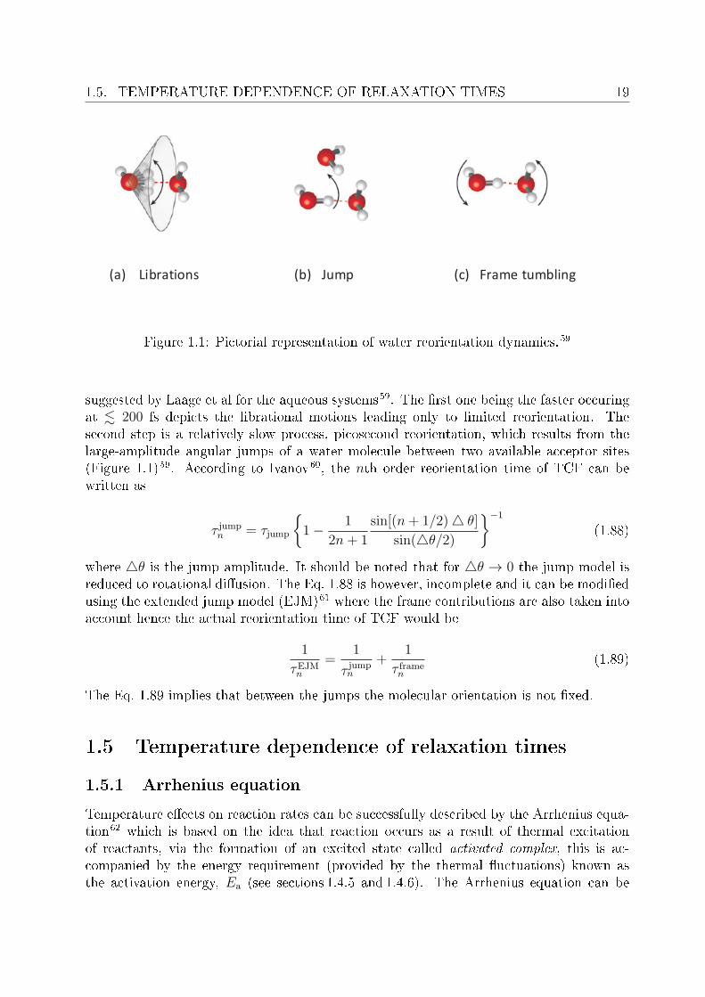
1.5. TEMPERATURE DEPENDENCE OF RELAXATION TIMES 19
(a) Librations (b) Jump (c) Frame tumbling
Figure 1.1: Pictorial representation of water reorientation dynamics.59
suggested by Laage et al for the aqueous systems59. The rst one being the faster occuringat . 200 fs depicts the librational motions leading only to limited reorientation. Thesecond step is a relatively slow process, picosecond reorientation, which results from thelarge-amplitude angular jumps of a water molecule between two available acceptor sites(Figure 1.1)59. According to Ivanov60, the nth order reorientation time of TCF can bewritten as
τ jumpn = τjump
1− 1
2n+ 1
sin[(n+ 1/2) θ]
sin(θ/2)
−1
(1.88)
where θ is the jump amplitude. It should be noted that for θ → 0 the jump model isreduced to rotational diusion. The Eq. 1.88 is however, incomplete and it can be modiedusing the extended jump model (EJM)61 where the frame contributions are also taken intoaccount hence the actual reorientation time of TCF would be
1
τEJMn
=1
τ jumpn
+1
τ framen
(1.89)
The Eq. 1.89 implies that between the jumps the molecular orientation is not xed.
1.5 Temperature dependence of relaxation times
1.5.1 Arrhenius equation
Temperature eects on reaction rates can be successfully described by the Arrhenius equa-tion62 which is based on the idea that reaction occurs as a result of thermal excitationof reactants, via the formation of an excited state called activated complex, this is ac-companied by the energy requirement (provided by the thermal uctuations) known asthe activation energy, Ea (see sections 1.4.5 and 1.4.6). The Arrhenius equation can be
20 CHAPTER 1. THEORETICAL BACKGROUND
modied for relaxation times as
ln τ = ln τ0 +Ea
RT(1.90)
Where Ea can be obtained through the slope and τ0, the pre-exponential factor representsthe intercept of the above straight line relation. Since increase in temperature results indecrease in observed relaxation times (due to increased dynamics of the related relaxationprocess) the τ0 value represents the minimum of τ for a relaxation process.
1.5.2 Eyring equation
A trivial equivalence to the Arrhenius equation is the transition state or Eyring equation63
which results from a theoretical model, based on transition state theory. Eyring equationcan be can be applied to study the temperature dependence of experimental relaxationtime, τ as
ln τ = lnh
kBT− ∆S =
R+
∆H =
RT(1.91)
where h is Planck's constant, R is the universal gas constant and ∆S = and ∆H = arerespectively the activation entropy and activation enthalpy. Equation 1.91 neglects thetemperature dependencies of ∆H = and ∆S = but extensions are possible, see reference64.The Gibbs energy of activation, ∆G =, can be calculated as
∆G = = ∆H = − T∆S = (1.92)
The quantities ∆H = and Ea can be interconverted via the thermodynamic relation
Ea = ∆H = +RT (1.93)
1.6 Solute-related relaxations
1.6.1 Ion-pair relaxation
The steady accretion of experimental data providing direct indication of ion-pairing hasput more stress to have a keen look into this phenomenon as its presence leaves visibleeects in many experimental techniques such as conductivity, potentiometry as well as onvarious thermodynamic parameters as osmotic coecient and activity coecient. Amongvarious spectroscopic techniques (UV-vis, IR, Raman and NMR), DRS has unique sensitiv-ity towards various types of ion pairs and DRS studies have been able to show ion pairingto some extent in virtually all classical strong electrolytes.10
Two Charged species, separated by a distance, d could be described as ion pairs if a < d < r,where a is the distance of closest approach and r is certain cuto distance, provided thatthe residence time of such pair at distance d is greater than the diusion time.65 This isessentially equivalent to the notion that, in order to detect ion pairs as distinct species insolution, their life time (τL = ln 2
kd, kd is the decay constant of ion pairs) should be atleast
1.6. SOLUTE-RELATED RELAXATIONS 21
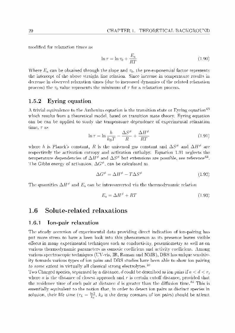
Figure 1.2: Eigen's scheme of stepwise ion association.67
comparable to the rotational correlation time. Literature reports values of ion-pair lifetimes of ∼ 1 ns.66 Ion association is mainly dependent on the ionic charges of the partnersand the solvent permittivity.
Cc+(aq) + Aa−(aq)hydrated free ions
KA CA0(aq)2SIP
(1.94)
Where KA is the equilibrium constant for the overall ion association. DRS detects ion-pairing even if its very weak i.e. for KA ≤ 1 M−1.10
On the basis of ultrasonic absorption data Eigen and Tamm suggested a multistep mech-anism (Figure 1.2) for the formation of ion pairs in aqueous solutions.67 This mechanismproceeds with the successive formation of dierent kinds of ion pairs as a result of com-petition between ion-solvent and ion-ion interactions. First stage of Eigen and Tammmechanism is essentially a diusion controlled reaction (very fast) and is associated withthe formation of double-solvent-separated ion pair (2SIP) or an outer-outer-sphere com-plex (both the ionic partners keep their solvation shells hence a double layer of solventmolecules intervene between the centers of cation and anion).
Cc+(aq) + Aa−(aq)hydrated free ions
K1 [Cc+(OH2)(OH2)Aa−](aq)
2SIP
(1.95)
Successive ejection of water molecules from 2SIP leads to the formation of a solvent-sharedion pair (SIP) or outer sphere complex (with single layer of solvent molecules betweencenters of two ionic partners, formation of SIP is slower than the 2SIP)
[Cc+(OH2)(OH2)Aa−](aq)
2SIP
K2 [Cc+(OH2)Aa−](aq)
SIP
(1.96)
nally in the last slowest step, total elimination of solvent molecules from SIP results intoa contact ion pair (CIP) or inner-sphere complex (cation and anion are in direct contact)
[Cc+(OH2)Aa−](aq)
SIP
K3 [CA](c−a)+(aq)CIP
(1.97)
Each of these three steps is characterized by its equilibrium constant, Ki, i = 1, 2, 3, andthe association constant KA = K1 +K1K2 +K1K2K3. Limited number of techniques areavailable to nd K1, K2 and K3, however conventional thermodynamic and conductivitymeasurements are able to nd KA.68,69 Depending on the solute concentration and relative
22 CHAPTER 1. THEORETICAL BACKGROUND
strength of ion-ion-, ion-solvent- and solvent solvent interactions, it is possible that theabove mentioned sequence of reactions stops at rst or second stage.11 Being dependenton the dipole moment of the species the sensitivity of DRS towards various ion-pair typesvaries in the order: 2SIP > SIP > CIP.11,65
DRS measurements allow the calculation of KA as
KA = cIP/(c− cIP)2 (1.98)
where cIP, in solution can be determined via Eqs. 1.72-1.78 (with j = IP). For the calcu-lation of AIP and µIP, geometrical parameters, the polarizability and the gas phase dipolemoment of the corresponding species should be known (which for the presented study arecalculated from the MOPAC). The obtained KA(I) can be tted in a Guggenheim-typeequation11 using I (≡ c for 1:1 electrolytes), the stoichiometric ionic strength as indepen-dent variable of the equation as
logKA = logKoA − 2ADH|z+z−|
√I
1 + AK
√I
+BKI + CKI3/2 (1.99)
where ADH is the Debye-Hückel coecient (0.5115 L1/2mol−1/2 for water at 25 C), andYK (Y = A, B, C) are adjustable parameters (AK is xed at 1.00 M−1/2 throughout forpresent studies).70
1.6.2 Ion-cloud relaxation
In solutions of electrolytes or charged colloids, any single ion can be viewed as chargedspecies surrounded by the ions of opposite charge (forming an oppositely charged ionic at-mosphere) due to long-range Coulombic interactions. Under the inuence of an electric eldions move in certain direction while the ionic atmosphere renews its position accordinglyin a nite time (ion-cloud relaxation), this eect was depicted by Debye and Falkenhagenin 192871. The presence of this ion-cloud has remarkable eects on the conductivities ofelectrolyte solutions mainly due to electrophoretic eect and time-of-relaxation eect.72
The relaxation time of ion-cloud relaxation mode is related to the molar conductivity ofelectrolyte at innite dilution, Λ∞, as22
τic =εεocΛ∞
(1.100)
Eq. 1.100 predicts a pronounced decrease of τic with increasing concentration of solute.Until recently, ion-cloud relaxation was neglected in the analysis of DRS spectra of elec-trolytes as its amplitude was thought to be small7375. Features in the 10 MHz to 1 GHzregion were commonly assigned to ion pairing only10. Via his theoretical model, Yam-aguchi et al76,77 found a low frequency composite mode (jointly arising from ion-cloudrelaxation and ion-pair reorientation) whose amplitude is very similar to the relaxationstrengths of the low-frequency modes, very often observed for 1:1 electrolytes. Thus thisprocess should be detectable by DRS as is observed for the aqueous solutions of NaCl78.However, up to date neither the theoretical approaches nor the experimental techniques
1.6. SOLUTE-RELATED RELAXATIONS 23
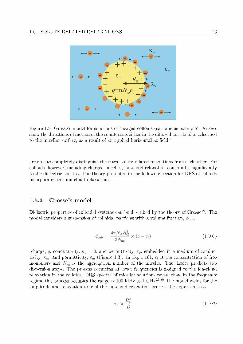
Figure 1.3: Grosse's model for solutions of charged colloids (cationic as example). Arrowsshow the directions of motion of the counterions either in the diused ion-cloud or adsorbedto the micellar surface, as a result of an applied horizontal ac eld.79
are able to completely distinguish these two solute-related relaxations from each other. Forcolloids, however, including charged micelles, ion-cloud relaxation contributes signicantlyto the dielectric spectra. The theory presented in the following section for DRS of colloidsincorporates this ion-cloud relaxation.
1.6.3 Grosse's model
Dielectric properties of colloidal systems can be described by the theory of Grosse79. Themodel considers a suspension of colloidal particles with a volume fraction, ϕmic,
ϕmic =4πNAR
3G
3Nag
× (c− cf) (1.101)
charge, q, conductivity, κp = 0, and permittivity, εp, embedded in a medium of conduc-tivity, κm, and permittivity, εm (Figure 1.3). In Eq. 1.101, cf is the concentration of freemonomers and Nag is the aggregation number of the micelle. The theory predicts twodispersion steps. The process occurring at lower frequencies is assigned to the ion-cloudrelaxation in the colloids. DRS spectra of micellar solutions reveal that, in the frequencyregime this process occupies the range ∼ 100 MHz to 1 GHz15,80 The model yields for theamplitude and relaxation time of the ion-cloud relaxation process the expressions as
τ1 ≈R2
G
D(1.102)

24 CHAPTER 1. THEORETICAL BACKGROUND
where RG and D are the eective Grosses's radius and diusion coecient of the counte-rions respectively.
S1 =9ϕmicεm(2χλs/κm)
4
16[2χλs
κm( 2λs
RGκm+ 1) + 2]2
(1.103)
In Eq. 1.103, λs denotes surface conductance whereas the parameter χ is related to Debyelength, χ−1 (characterizes the size of ion cloud) which can be written as
χ−1 =
√εoεmD
κm
(1.104)
The process occurring at relatively higher frequencies reects the interfacial polarizationat the micelle/solvent boundary and it results from the tangential motion of the boundcounterions. The relaxation time of this process can be written as
τ2 =εoεm(
εpεm
+ 2)
κm(2λs
RGκm+ 2)
(1.105)
whereas its amplitude can be dened as
S2 =9ϕmicεm(
2λs
RGκm− εp
εm)2
( εpεm
+ 2)( 2λs
RGκm+ 2)2
(1.106)
The relaxation times (τ1 and τ2) and amplitudes (S1 and S2) are derived by assuming thatϕmic is small and RG ≫ χ−1.
Chapter 2
Experimental
2.1 Sample preparation
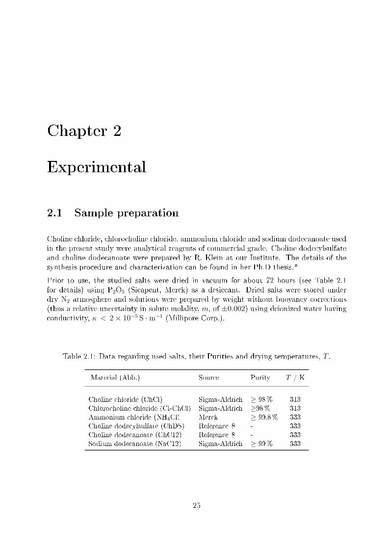
Choline chloride, chlorocholine chloride, ammonium chloride and sodium dodecanoate usedin the present study were analytical reagents of commercial grade. Choline dodecylsulfateand choline dodecanoate were prepared by R. Klein at our Institute. The details of thesynthesis procedure and characterization can be found in her Ph.D thesis.8
Prior to use, the studied salts were dried in vacuum for about 72 hours (see Table 2.1for details) using P2O5 (Sicapent, Merck) as a desiccant. Dried salts were stored underdry N2 atmosphere and solutions were prepared by weight without buoyancy corrections(thus a relative uncertainty in solute molality, m, of ±0.002) using deionized water havingconductivity, κ < 2× 10⁻⁵ S ·m−1 (Millipore Corp.).
Table 2.1: Data regarding used salts, their Purities and drying temperatures, T .
Material (Abb.) Source Purity T / K
Choline chloride (ChCl) Sigma-Aldrich ≥ 98% 313Chlorocholine chloride (Cl-ChCl) Sigma-Aldrich ≥98% 313Ammonium chloride (NH4Cl) Merck ≥ 99.8% 333Choline dodecylsulfate (ChDS) Reference 8 - 333Choline dodecanoate (ChC12) Reference 8 - 333Sodium dodecanoate (NaC12) Sigma-Aldrich ≥ 99% 333
25

26 CHAPTER 2. EXPERIMENTAL
2.2 Measurement of dielectric properties
2.2.1 Time-domain reectometry
Dielectric data in the low frequency regime (down to few MHz) is of great importance tostudy the fundamental aspects of structure and dynamics in liquids, in this regard timedomain reectometry (TDR) is capable of determining the dielectric properties of liquidsat MHz to low GHz frequencies. The measurement cell (Figure 2.1) consist of coaxialline terminated by a coaxial line of dierent dimensions, where the insulating materialis replaced by the sample. Ideally, the outer conductor is innitely continued, while theinner conductor has a certain length, l. At the end of the inner conductor, a coaxial tocircular waveguide transition is the electromagnetic boundary condition.81 Due to a step inthe impedance at the coaxial-line sample cell transition, an electromagnetic wave is partlyreected. The complex permittivity measurements are based on the determination of thecomplex reection coecients at this impedance step.82
Figure 2.1: A cut-o type reection cell:82 1 0.085′′semi-rigid feeding line with ange, 2
cell base plate with 3 soldered hermetic feed through, 4 inner conductor of diameter d1and length l, 5 cell body with gold-plated bore 5a as outer conductor of diameter d2, 6Swage-Lockr tting, 7 tting capillary.
Theory A fast rising voltage pulse, Vo(t), is applied to the sample. The pulse propagatingin the sample is deformed according to the dielectric properties of the sample, and reectedsignal, Vr(t), is obtained. The shape of Vo(t), registered by a fast sampling scope, is then

2.2. MEASUREMENT OF DIELECTRIC PROPERTIES 27
compared to Vr(t). Fourier transformation of the time-dependent intensities of the signalyields the intensities in the frequency domain, υo(ω) and υr(ω):
υo(ω) = Liω
[d
dtVo(t)
]=
∞∫0
d
dtVo(t) · exp(iωt)dt (2.1)
υr(ω) = Liω
[d
dtVr(t)
]=
∞∫0
d
dtVr(t) · exp(iωt)dt (2.2)
Eq. 2.1 and 2.2 can be used to calculate the absolute complex reection coecient of thecell, ρ(ω),
ρ(ω) =coiωgl
· υo(ω)− υr(ω)
υo(ω) + υr(ω)(2.3)
in the above equation l is the pin-length of the inner conductor and g is the ratio between thewave resistance of the empty cell and the feeding line. Due to fringing elds at the coaxialline to waveguide transition the eective pin length, lel, slightly exceeds the mechanicalpin length, l, hence in Eq. 2.3 lel is used. Within some approximations, the generalizedcomplex dielectric permittivity, η(ω), can be obtained from ρ(ω) by the numerical solutionof,
η(ω) = ρ(ω) · z cot z (2.4)
wherez =
ωl
co
√η(ω) (2.5)
It should be noted that, the incident wave is not easily accessible from the measurement.Therefore, a sample of known (and preferably similar) dielectric properties is used asreference, and the relative reection coecient is determined as
ρxr(ω) =c
iωgl·Liω
[ddtVrr(t)
]− Liω
[ddtVrx(t)
]Liω
[ddtVrr(t)
]+ Liω
[ddtVrx(t)
] (2.6)
In Eq. 2.6, Vrx(t) and Vrr(t) represent the relative time dependent reection intensities ofthe sample and the reference, respectively.83,84 The relative reection coecient is relatedto the dielectric properties by the working equation,
ρxr =ηx · zr cot(zr)− ηr · zx cot(zx)
zr cot(zr)zx cot(zx) + g2 · ηxηr(ωl/c)2(2.7)
with
zx =ωl
c
√ηx and zr =
ωl
c
√ηr (2.8)
Numerical solution of Eq. 2.7 with a Newton-Raphson procedure and Tailor series expan-sion of z · cot z yields ηx(ω).85
28 CHAPTER 2. EXPERIMENTAL
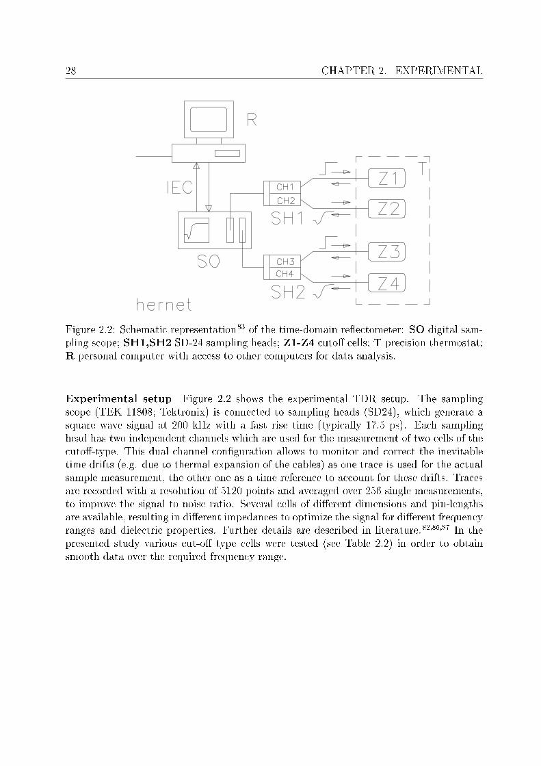
Figure 2.2: Schematic representation83 of the time-domain reectometer: SO digital sam-pling scope; SH1,SH2 SD-24 sampling heads; Z1-Z4 cuto cells; T precision thermostat;R personal computer with access to other computers for data analysis.
Experimental setup Figure 2.2 shows the experimental TDR setup. The samplingscope (TEK 11808; Tektronix) is connected to sampling heads (SD24), which generate asquare wave signal at 200 kHz with a fast rise time (typically 17.5 ps). Each samplinghead has two independent channels which are used for the measurement of two cells of thecuto-type. This dual channel conguration allows to monitor and correct the inevitabletime drifts (e.g. due to thermal expansion of the cables) as one trace is used for the actualsample measurement, the other one as a time reference to account for these drifts. Tracesare recorded with a resolution of 5120 points and averaged over 256 single measurements,to improve the signal to noise ratio. Several cells of dierent dimensions and pin-lengthsare available, resulting in dierent impedances to optimize the signal for dierent frequencyranges and dielectric properties. Further details are described in literature.82,86,87 In thepresented study various cut-o type cells were tested (see Table 2.2) in order to obtainsmooth data over the required frequency range.
2.2. MEASUREMENT OF DIELECTRIC PROPERTIES 29
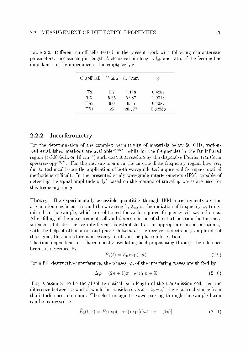
Table 2.2: Dierent cuto cells tested in the present work with following characteristicparameters: mechanical pin-length, l, electrical pin-length, lel, and ratio of the feeding lineimpedance to the impedance of the empty cell, g.
Cuto cell l/ mm lel/ mm g
T9 0.7 1.118 0.4282TX 5.35 5.987 1.0018TS3 6.0 6.05 0.4282TS1 25 26.377 0.82258
2.2.2 Interferometry
For the determination of the complex permittivity of materials below 50 GHz, variouswell established methods are available25,88,89 while for the frequencies in the far infraredregion (>300 GHz or 10 cm−1) such data is accessible by the dispersive Fourier transformspectroscopy90,91. For the measurements in the intermediate frequency region however,due to technical issues the application of both waveguide techniques and free space opticalmethods is dicult. In the presented study waveguide interferometers (IFM, capable ofdetecting the signal amplitude only) based on the method of traveling waves are used forthis frequency range.
Theory The experimentally accessible quantities through IFM measurements are theattenuation coecient, α, and the wavelength, λm, of the radiation of frequency, ν, trans-mitted in the sample, which are obtained for each required frequency via several steps.After lling of the measurement cell and determination of the start position for the mea-surement, full destructive interference is established at an appropriate probe position z
′0
with the help of attenuators and phase shifters, as the receiver detects only amplitude ofthe signal, this procedure is necessary to obtain the phase information.The time-dependence of a harmonically oscillating eld propagating through the referencebeams is described by
E1(t) = E0 exp(iωt) (2.9)
For a full destructive interference, the phases, φ, of the interfering waves are shifted by
∆φ = (2n+ 1)π with n ∈ Z (2.10)
If z0 is assumed to be the absolute optical path length of the transmission cell then thedierence between z0 and z
′0 would be considered as x = z0− z′0, the relative distance from
the interference minimum. The electromagnetic wave passing through the sample beamcan be expressed as
E2(t, x) = E0 exp(−αx) exp [i(ωt+ π − βx)] (2.11)

30 CHAPTER 2. EXPERIMENTAL
where β = 2π/λm is the phase coecient. Since both reference and sample beams arecombined at the receiver, their superposition yields
E(t, x) = E1(t) + E2(t, x) = E0 exp(iωt) [1 + exp(−αx) exp(i(π − βx))] (2.12)
The power P of the detected signal is experimentally accessible and is dened as
P = E · E∗ = E20 · I(x) (2.13)
where E0 is the amplitude of E and I(x) is the interference function, which can be denedas
I(x) = [1 + exp(−αx) exp(i(π − βx))] · [1 + exp(−αx) exp(i(π − βx))] (2.14)
= 1 + exp(−2αx) + exp(−αx) · 2 cos(−π + βx) (2.15)
The signal-level measured by the receiver, A(x), is commonly expressed in decibel (dB),i.e. the relative attenuation of the signal power on a logarithmic scale. It is dened as
A(x) = 10 lgP (x)
Pref
(2.16)
Since Pref is not known, A(x) is normalized by A0, the relative intensity of the signalpassing through the sample beam at position z′0
A0 = 10 lgP0
Pref
(2.17)
and it follows
Arel(x) = A(x)− A0
= 10 lgP (x)
Pref
− 10 lgP0
Pref
= 10 lgP (x)
P0
= 10 lgE2
0 · I(x)E2
0
(2.18)
The recorded interferogram A(z0 − z′0) can be tted by the expression92
A(z0 − z′0) = A0 + 10 lg
1 + exp [−2pαdB(z0 − z′0)]
− 2 cos
(2π
λm
(z0 − z′0)
)· exp [−pαdB(z0 − z′0)]
(2.19)
In above equation p is a conversion factor
p =
(20 lg e · dB
Np
)−1
(2.20)

2.2. MEASUREMENT OF DIELECTRIC PROPERTIES 31
Eq. 2.19 yields the power attenuation coecient, αdB (in dB/m), and λm. These quantitiesare related to η(ν) via
η′(ν) =(c0ν
)2 [( 1
λvacc,10
)2
+
(1
λm(ν)
)2
−(α(ν)
2π
)2]
and (2.21)
η′′(ν) =(c0ν
)2 α(ν)
πλm(ν)(2.22)
Where λvacc,10 is the limiting vacuum frequency, a characteristic quantity for a particular
waveguide.
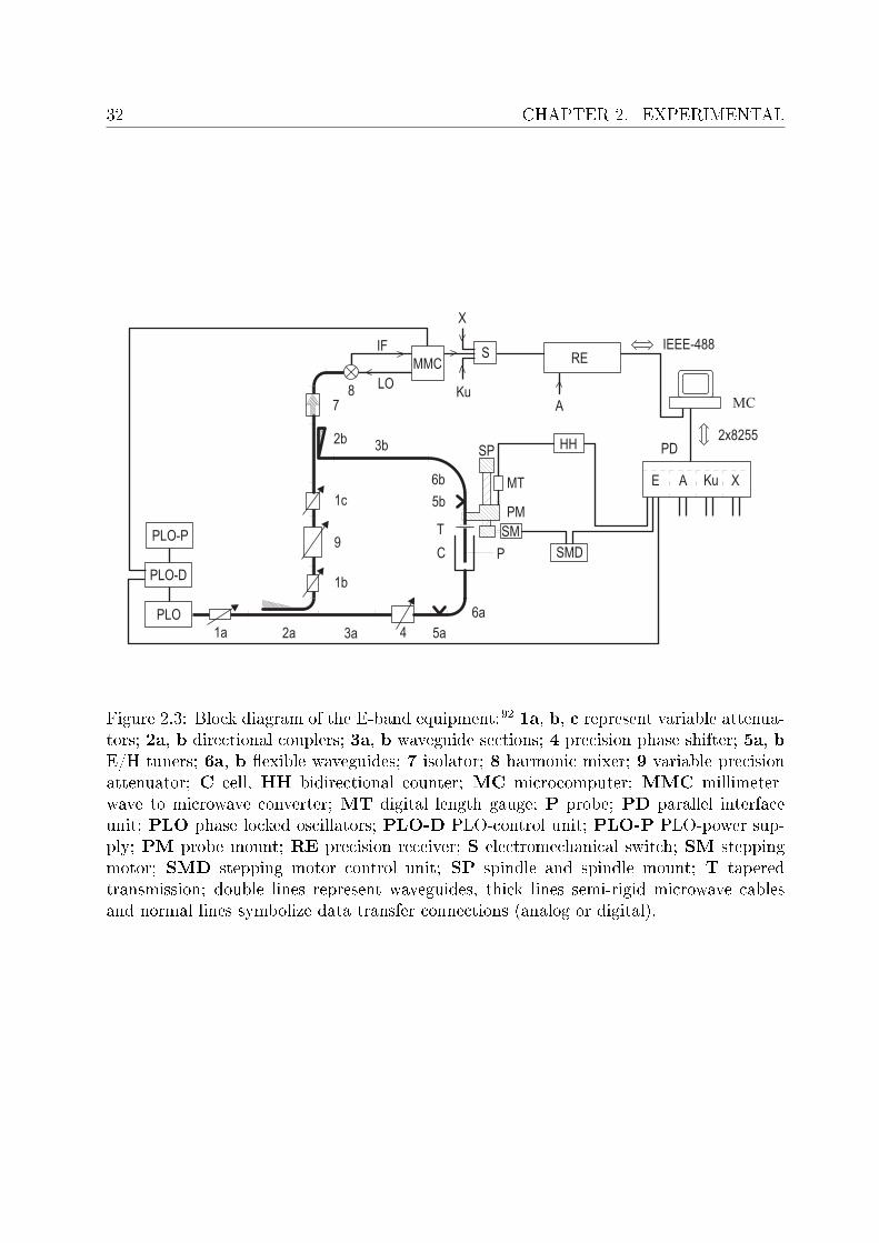
Experimental setup Figure 2.3 shows a block diagram of the E-band setup where acomputer-controlled system of transmission lines is used. Phase lock oscillators are usedto generate signals of desired frequency. The signal coming from the source is then split bya directional coupler to feed the measuring and reference branches. The sample is placedin a cell consisting of mica window, a piece of waveguide and a gold-plated (5 µm, tosuppress corrosion) ceramic probe with variable, motor-controlled position. Variable preci-sion phase shifters and attenuators are integrated in the branches. Signals are recombinedby directional couplers and then after passing through the isolator, harmonic mixer andmillimeterwave to micrometerwave converter the signal is detected at a precision attenua-tion receiver. Two types of double-beam interferometers were used for measurement of thedielectric properties at high GHz frequencies92 namely A-band (27 ≤ ν/GHz ≤ 40) andE-band (60 ≤ ν/GHz ≤ 89). For the A-band measurements, however interferometer wasconnected to the VNA (see section 2.2.3) to enable continuous frequency scans93, whereasthe temperature was controlled by a Julabo FP 50 or a Lauda RK 20 thermostat andmonitored by a Pt-100 resistance with a precision of ±0.02 C and an overall accuracy of±0.05 C. Prior to the lling the cells were properly washed and dried with a spray of drynitrogen. It should be noted that the IFM measurements do not require any calibrationand the obtained data is considered absolute.
32 CHAPTER 2. EXPERIMENTAL
Figure 2.3: Block diagram of the E-band equipment:92 1a, b, c represent variable attenua-tors; 2a, b directional couplers; 3a, b waveguide sections; 4 precision phase shifter; 5a, bE/H tuners; 6a, b exible waveguides; 7 isolator; 8 harmonic mixer; 9 variable precisionattenuator; C cell, HH bidirectional counter; MC microcomputer; MMC millimeter-wave to microwave converter; MT digital length gauge; P probe; PD parallel interfaceunit; PLO phase locked oscillators; PLO-D PLO-control unit; PLO-P PLO-power sup-ply; PM probe mount; RE precision receiver; S electromechanical switch; SM steppingmotor; SMD stepping motor control unit; SP spindle and spindle mount; T taperedtransmission; double lines represent waveguides, thick lines semi-rigid microwave cablesand normal lines symbolize data transfer connections (analog or digital).
2.2. MEASUREMENT OF DIELECTRIC PROPERTIES 33
2.2.3 Vector network analysis
Due to the need of maximum power transfer at higher frequencies, the coaxial lines arepreferably used. Commercially available devices (vector network analyzers, VNA, capableof analyzing both magnitude and phase of the component signals in electrical networks) areable to operate upto 110 GHz. For the characterization of a two-port device, an arbitraryelectrical network is analyzed by determining the reection and transmission of electricalsignals which yields the scattering parameter matrix, S, that can be dened as(
b1b2
)=
(S11 S12
S21 S22
)(a1a2
)where aj and bj are the incident and reected power waves at the port j, respectively.For one-port measurements (reection studies) the instrument has to be calibrated withat least three reference materials (conventionally open, short and 50 Ω are used) in orderto correct the errors in directivity, ed, frequency response, er, and source match, es. Theobtained scattering parameter by the VNA, Sm
jj can be dened as
Smjj = ed +
erSajj
1− esSajj
(2.23)
where Sajj is the actual scattering parameter at the plane of interest.
For one-port reection measurements on an electrical network, consisting of an impedancestep varying from Z1 to Z2, the complex scattering parameter S11, is dened as
S11 =1− Y
1 + Y(2.24)
In Eq. 2.24, Y = Z2/Z1, is the normalized terminating impedance.
Open-ended coaxial probes
Dielectric data of aqueous solutions of ChCl, ClChCl, NH4Cl, ChC12, ChDS, and NaC12,in the frequency range 0.2 ≤ ν/GHz≤ 50 was recorded with Agilent E8364B VNA con-nected to an electronic calibration module (Ecal, Agilent N4693A) and a dielectric probekit (85070E). The use of Ecal module ensures the eciency and accuracy of VNA setupas it measures the well known reection standards during the measurement and thuscompensates for the systematic drifts, e.g., phase error due to possible thermal expan-sion of the coaxial lines. This setup requires the use of two dierent open-ended coaxialprobes namely high temperature probe and performance probe in the frequency range0.2 ≤ ν/GHz≤ 20 (with 61 equidistant frequency data points on logarithmic scale) and1 ≤ ν/GHz≤ 50 (with 51 equidistant frequency data points on logarithmic scale), respec-tively (in principle the frequency limit of theses probes is 0, but due to small aperture

34 CHAPTER 2. EXPERIMENTAL
capacitances data were practically reproducible down to 0.2 GHz and 1 GHz for high tem-perature and performance probe, respectively). However, during the tting procedure, inorder to have an equal density of data points throughout, the data of the performance probewas used in frequency range 15 . ν/GHz≤ 50 only. Both probe heads were mounted intwo dierent temperature controlled cells as described by Hunger.93 The temperature wascontrolled with a Huber CC505 thermostat and measured with a Agilent 34970A datalog-ger, using a platinum resistance thermometer (PT-100) in 4-wire conguration.The complex dielectric parameter η was calculated from the normalized aperture impe-dence of the probe head, Y by using a simplied coaxial aperture opening model94,95 andnumerical solution of the equation
Y =ik2
πkc ln(D/d)
[i
(I1 −
k2I32
+k4I524
− k6I7720
+ ...
)+
(I2k − k3I4
6+
k5I6120
− ...
)](2.25)
In Eq. 2.25, kc = ω√ηcε0µ0 and k = ω
√ηε0µ0 are the propagation constants within the
dielectric material of the coaxial probe head (index c) and within the sample, respectively.A theoretical approach yields the probe constants I1 . . . I28 95, whereas D and d are radii ofouter and inner conductor of coaxial line, respectively.Calibration of the VNA was performed according to Eq. 2.23 with respect to the probe-sample interface. A standard three point calibration using air (open), mercury (short)and a pure liquid (load, with accurately known dielectric properties) was used. Prior touse mercury was puried according to the procedure described by Wölbl;96 minor scumformation was removed by `pin-hole' ltration (paper lter). Since dielectric propertiesof the third calibration material should be close to those of the studied sample so, waterwas adopted as a third reference material. At least two independent calibrations wereperformed (for each probe head type) to obtain a set of consistent spectra for each of thestudied system.
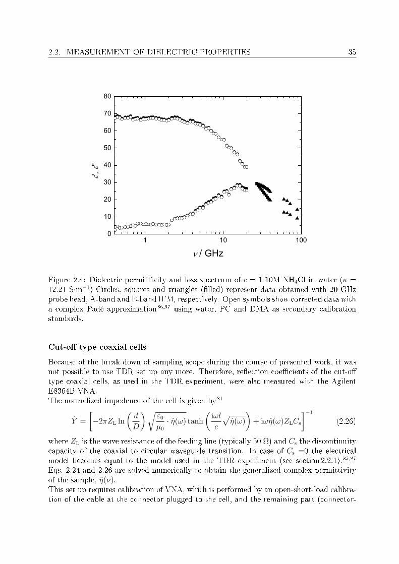
Generally a complex Padé approximation,86,97 is used for the correction of VNA data, if thedielectric properties of the sample deviate considerably from that of reference liquid. Thisapproach was also tested in the present studies for the selected systems, using water, propy-lene carbonate (PC, Sigma-Aldrich, 99.7%) and N,N -dimethylacetamide (DMA, Fluka,> 99.8%) as secondary calibration standards. No signicant improvement of the VNAspectra was observed after doing Padé calibration (Figure 2.4), in addition the uncorrecteddata was in excellent agreement with the corresponding IFM measurements (absolute data,do not require any calibration), so this approximation was not applied to the presentedstudies.
2.2. MEASUREMENT OF DIELECTRIC PROPERTIES 35
1 10 1000
10
20
30
40
50
60
70
80
',
''
/ GHz
Figure 2.4: Dielectric permittivity and loss spectrum of c = 1.10M NH4Cl in water (κ =12.21 S·m−1) Circles, squares and triangles (lled) represent data obtained with 20 GHzprobe head, A-band and E-band IFM, respectively. Open symbols show corrected data witha complex Padé approximation86,97 using water, PC and DMA as secondary calibrationstandards.
Cut-o type coaxial cells
Because of the break down of sampling scope during the course of presented work, it wasnot possible to use TDR set up any more. Therefore, reection coecients of the cut-otype coaxial cells, as used in the TDR experiment, were also measured with the AgilentE8364B VNA.The normalized impedence of the cell is given by81
Y =
[−2πZL ln
(d
D
)√ε0µ0
· η(ω) tanh(iωl
c
√η(ω)
)+ iωη(ω)ZLCs
]−1
(2.26)
where ZL is the wave resistance of the feeding line (typically 50 Ω) and Cs the discontinuitycapacity of the coaxial to circular waveguide transition. In case of Cs =0 the electricalmodel becomes equal to the model used in the TDR experiment (see section 2.2.1).85,87
Eqs. 2.24 and 2.26 are solved numerically to obtain the generalized complex permittivityof the sample, η(ν).This set up requires calibration of VNA, which is performed by an open-short-load calibra-tion of the cable at the connector plugged to the cell, and the remaining part (connector-
36 CHAPTER 2. EXPERIMENTAL
0.01 0.10.3
0.4
0.5
0.6
0.7
0.8
0.9
1.0
S
11
/ GHz
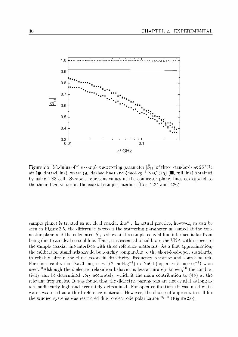
Figure 2.5: Modulus of the complex scattering parameter |S11| of three standards at 25 C :air ( , dotted line), water (N, dashed line) and 5mol·kg−1 NaCl(aq) (, full line) obtainedby using TS3 cell. Symbols represent values at the connector plane, lines correspond tothe theoretical values at the coaxial-sample interface (Eqs. 2.24 and 2.26).
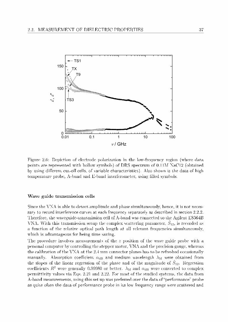
sample plane) is treated as an ideal coaxial line81. In actual practice, however, as can beseen in Figure 2.5, the dierence between the scattering parameter measured at the con-nector plane and the calculated S11 values at the sample-coaxial line interface is far frombeing due to an ideal coaxial line. Thus, it is essential to calibrate the VNA with respect tothe sample-coaxial line interface with three reference materials. As a rst approximation,the calibration standards should be roughly comparable to the short-load-open standards,to reliably obtain the three errors in directivity, frequency response and source match.For short calibration NaCl (aq, m ∼ 0.2 mol·kg−1) or NaCl (aq, m ∼ 5 mol·kg−1) wereused.98Although the dielectric relaxation behavior is less accurately known,98 the conduc-tivity can be determined very accurately, which is the main contribution to η(ν) at therelevant frequencies. It was found that the dielectric parameters are not crucial as long asκ is suciently high and accurately determined. For open calibration air was used whilewater was used as a third reference material. However, the choice of appropriate cell forthe studied systems was restricted due to electrode polarization99,100 (Figure 2.6).
2.2. MEASUREMENT OF DIELECTRIC PROPERTIES 37
0.01 0.1 1 10 1000
50
100
150TS1
T9TX
',
''
/ GHz
TS3
Figure 2.6: Depiction of electrode polarization in the low-frequency region (where datapoints are represented with hollow symbols) of DRS spectrum of 0.11M NaC12 (obtainedby using dierent cut-o cells, of variable characteristics). Also shown is the data of hightemperature probe, A-band and E-band interferometer, using lled symbols.
Wave guide transmission cells
Since the VNA is able to detect amplitude and phase simultaneously, hence, it is not neces-sary to record interference curves at each frequency separately as described in section 2.2.2.Therefore, the waveguide-transmission cell of A-band was connected to the Agilent E8364BVNA. With this transmission setup the complex scattering parameter, S12, is recorded asa function of the relative optical path length at all relevant frequencies simultaneously,which is advantageous for being time saving.The procedure involves measurements of the z position of the wave guide probe with apersonal computer by controlling the stepper motor, VNA and the precision gauge, whereasthe calibration of the VNA at the 2.4 mm connector planes has to be refreshed occasionallymanually. Absorption coecient αdB and medium wavelength λM were obtained fromthe slopes of the linear regression of the phase and of the magnitude of S12. Regressioncoecients R2 were generally 0.99980 or better. λM and αdB were converted to complexpermittivity values via Eqs. 2.21 and 2.22. For most of the studied systems, the data fromA-band measurements, using this set up was preferred over the data of performance probeas quite often the data of performance probe in its low frequency range were scattered and

38 CHAPTER 2. EXPERIMENTAL
the scattering become worst for the data at high temperatures and for high conductingsamples, this surely depicts the need for having some appropriate calibration materials(with κ >> 0) for the highly conducting systems.
2.2.4 Data analysis
Once the dielectric data at the spot frequencies are obtained, a frequency-continuous de-scription via a suitable model has to be found. It is preferred to analyze ε(ν) data aftercorrecting for dc conductivity rather than η(ν) as this may lead to biasing of the resultingparameters, due to large values of η′′ at low ν as weights are higher at low ν than at high ν.Therefore, the spectra were rst corrected for the measured conductivity, κ, as a startingapproximation. The κ was varied slightly in order to improve the t quality (Eq. 2.27).The dierence between the experimental conductivity from low-frequency measurements inthe Hz-kHz region and adjusted κ values reects errors in the measurement setup and/orin mathematical model for the equipment.101,102
Furthermore, the measured data triples (νi, ε′i, ε′′i ) have to be tted by the relaxation
models (or superpositions) as already described in preceding chapter. However, due tothe broadness of relaxation modes in the condensed phase nding the right model is nottrivial, and also the successful formal description does not automatically imply that theresolved modes have a physical meaning or that they are independent of each other. Thus,few basic rules should be obeyed:Firstly, the parameters obtained have to be physically meaningful. Second, the normalizedvariance of the t, χ2
r , dened as
χ2r =
1
2N −m− 1
[N∑i=1
wε′(νi)δε′(νi)
2 +N∑i=1
wε′′(νi)δε′′(νi)
2
](2.27)
should be small. In above equation, δε′(νi) and δε′′(νi) are the residuals, N is the numberof data triples [νi, ε′(νi), ε′′(νi)] and m the number of the adjustable parameters; wε′(νi)and wε′′(νi) are the weights; only unweighted ts, wε′(νi) = wε′′(νi) = 1, were performedin the analysis of the spectra presented here.Additionally, the number of parameters should be as small as possible and the relaxationmodel should not vary in a concentration or temperature series measurements, unless thereare some specic physical reasons.It should also be noted that the model seeming to be most appropriate for a studied systemcan depend on the measured frequency range as well as on the precision and the densityof the spot frequency, hence special care should be taken regarding the density, meaningthat the number of data points should be comparable over the whole frequency range.Dierent relaxation models were tested for each of the studied systems in the presentedwork, by simultaneously tting ε′(ν) and ε′′(ν) (as is advisable) using the MWFIT program.A non-linear least-squares routine based on the method of Levenberg and Marquardt is usedin this program.103 However, due to the nonlinear nature of the tting process, assignmentof statistically meaningful standard uncertainties to the individual t parameters is notpossible but the square root of the diagonal elements of the covariance matrix can be usedas a measure for the certainty of the resulting parameters.103,104

2.2. MEASUREMENT OF DIELECTRIC PROPERTIES 39
In order to further check the validity of an accepted model, another tting procedure andcomputer code was used for the evaluation of a discrete analog of relaxation time distribu-tion functions105. Due to unbiased nature of this tting technique no prior knowledge ofnumber of modes, characteristic times of the modes, relaxation amplitudes or the relaxationtime distribution function is required for the Zasetsky method. This tting procedure isbased on a quasi-linear procedure with constraints for least squares tting of experimentalcomplex dielectric permittivity spectra in the frequency domain. The solution of linearleast square minimization problem with constraints105,106 provides information on relax-ation time distribution functions. The procedure involves the linearization of non-linearleast square tting of dielectric spectra by pre-computing (based on the Debye model ofrelaxation) a set of basis spectra, modications can be done for the non-debye type re-laxation modes105. However, it must be noted that both of the above mentioned ttingroutines do not a priori reect the actual molecular level mechanism behind the resolvedrelaxation modes.
40 CHAPTER 2. EXPERIMENTAL
2.3 Auxiliary measurements
2.3.1 Densimetry
Solution densities, ρ, were measured with an accuracy of ∼ ±0.05 kg·m−3 using a vibrating-tube densimeter (Anton Paar DMA 60/601 HT) according to the method described inliterature107. The instrument measures the period of vibration, τ , of a glass tube lledwith the sample. Sample density is related to this τ as
ρ = A×(τ 2 − B
)(2.28)
where A and B are the intrument-related constants that were determined via calibra-tion using degassed Millipore MILLI-Q water and puried nitrogen at atmospheric pres-sure, assuming densities from standard sources108. The temperature was kept constant to±0.003 C with an overall accuracy of ±0.02 C using a Braun Thermomix 1480 thermostatin combination with a thermostated heat sink (Lauda RK 20).However, later on due to availablity of new instrument, the densities for rest of studiedsystems were measured with a densimeter DMA 5000 M (Anton Paar), which measures τof a U-shaped borosilicate glass tube lled with the sample, for this instrument τ is relatedto the ρ as
ρ = A×(
τ
τref
)2
× f1 − B× f2 (2.29)
where τref is the period of oscillation of the reference oscillator, A and B are the instrumentconstants, and f1 and f1 are the correction terms for temperature, viscosity and nonlinearity,respectively.The temperature was kept constant to ±0.001 C with an overall accuracy of ±0.01 Cwith a built-in thermoelectric temperature control. The precision of the measurements was±0.001 g·L−1. The accuracy stated by the manufacturer is ±0.005 g·L−1. Before startingactual measurements water check was performed to check the accuracy while air checkwas performed quite often to ensure that the measuring cell was clean and properly dried.The obtained density data (at 25 C) was used to calculate molar concentrations, c, of thestudied systems, in addition for ChCl(aq), ClChCl(aq) and NH4Cl(aq) ρ were recordedat 5 C, 15 C, 25 C, 35 C and 45 C for various concentrations of each electrolyte. ForChCl(aq) and ClChCl(aq) such data was used to calculate apparent molar volume, ϕv.
2.3.2 Conductivity
For the determination of electrical conductivities, κ, the Wheatstone-bridge equipmentdescribed previously,109111 was used (with precision of ±0.2% and an accuracy of ±0.5%).The temperature was controlled with a home-built precision thermostat stable to ±0.003Kin combination with a thermostated heat sink (Lauda Kryomat K 90 SW). A set of dierenttwo-electrode capillary cells with cell constants, C, ranging from 25 to 360 cm−1 were used.The cells were calibrated with aqueous solutions of KCl.112 The cell resistance, R(ν),was measured manually as a function of the applied AC frequency, ν, between 120Hzand 10 kHz. To overcome possible eects of electrode polarization, the conductivity of
2.3. AUXILIARY MEASUREMENTS 41
each sample was obtained as κ = C/R∞ where R∞ = limν→∞R(ν) was obtained byextrapolation using the empirical function R(ν) = R∞ + A/νa, where A is specic to thecell and a was found to be in the range 0.5 . a . 1.113
Later on, another computer-controlled setup for the conductivity measurements was es-tablished in our lab and was used to record the conductivity data for some of the studiedsystems114. This setup involves use of a Huber, unistat 705 as the thermostat (tem-perature stability < 0.005K), a high-precision LCR-bridge∗ (HAMEG, HM8118) for themeasurement of R(ν) (relative uncertainty ≤ 0.0005), and a switchboard to address thecapillary cells mounted on the thermostat lid. Parasitic impedances were eliminated by anopen/short calibration of LCR-bridge and switchboard prior to each measurement.Measurement temperatures were recorded with an uncertainty of ±0.01K with a MISTtraceable Pt-100 resistance thermometer (ASL). The conductivities were obtained in thesame way as mentioned above.
2.3.3 Viscometry
The dynamic viscosities, η, of aqueous solutions (of selected systems) were measured usingan automated rolling-ball viscometer (Anton Paar AMVn) at 5 C, 15 C, 25 C, 35 C and45 C (with a temperature uncertainty ≤ 0.01K) as
η = K1 × (ρK − ρ)× t1 (2.30)
where K1 is the calibration constant of the measuring system, ρK is the density of thefalling ball, ρ is the density of the measured sample and t1 is the the rolling time of theball.The manufacturer-stated relative uncertainty of the instrument is ≤ 0.005. The repeata-bility and reproducibility of the viscosity measurements are < 0.1% and < 0.5%, respec-tively.
2.3.4 MOPAC calculations
In order to validate the experimental results pertaining to molecular properties, semiem-pirical quantum mechanical calculations (MOPAC2009115) were performed for various ionsand ion-pairs using the PM6 Hamiltonian.116 Dipole moments were calculated assumingthe geometric center (i.e. the center of the longest axis of the ion/ion-pair) as pivot. Thegeometry of the ions was optimized using the eigenvector-following (EF) routine117 and forthe ion-pairs, in order to avoid geometry reorganization, the 1SCF method was preferablyused. Molecular diameters, dmax, were obtained by taking the longest distance betweentwo atoms and adding the Van der Waals radii of the atoms118, whereas the Van der Waalsvolumes, VvdW, were obtained from the optimized geometry of the ions/ion-pairs usingWINMOSTAR119.
∗The measurable frequency range of the LCR-bridge is from 20Hz to 200 kHz.


Chapter 3
Investigation of electrolyte solutions
Knowledge pertaining to ion-association and ion-hydration is crucial in determining variousproperties of electrolyte solutions which in case of biological ions, can be correlated tovarious ongoing processes in living systems. Thus, whether it be strong ion-ion interactions(resulting in ion-pairing or aggregation) or strong ion-solvent interactions (giving rise to aspecic hydration pattern), both are the area of peculiar interest for electrolyte solutionchemists, so a huge body of data is available on these phenomena, and their importance inareas ranging from geochemistry to various biological processes and large scale technicalapplications has been widely recognized.120,121
Present work deals with the study of ammonium (NH+4 ), choline (Ch+, chemically 2-
hydroxyethyl trimethyl ammonium ion, vitamin B4) and chloro-choline ion (Cl-Ch+, 2-chloroethyl trimethyl ammonium ion) through dielectric relaxation spectroscopy (DRS).Solvation studies of NH+
4 ion are important in the environmental chemistry of pollutantsand soil contamination122 in addition NH+
4 ion is an important chemical species that servesas a simple model for solvated amides123,124 while high-temperature density data of NH4Clis needed for the problem of material transport and solid deposition in steam generatorsystems.125
Choline is an important dietary component2,3 which is required for the normal brain func-tioning in human. Moreover choline keeps the constituency of cell membranes, is involvedin cholinergic neurotransmission4 and is an important part of pulmonary surfactants.126
Recently choline based ionic liquids9 and surfactants127,128 have attracted increased atten-tion in many elds. It is also known to form a deep eutectic solvent (DES) with urea,129
and Chloro-choline chloride is known to be an eective plant growth regulator.130
Since the structure and functioning of biomolecules mainly depend on the presence andstructuring of water molecules around them so it is of crucial importance to study theproperties of these molecules in aqueous environment. As far as the study of hydrationbehaviour of biomolecules is concerned several techniques, each having its own limitationshave been employed so far. Nuclear magnetic resonance (NMR) and X-ray diractionare powerful techniques to study the specic hydration sites with atomic resolution.131133
Calorimetry studies mainly deal with the macroscopic amount of water and solute and lacksthe data at the molecular level.134,135 In contrast to bulk methods such as calorimetry, X-ray crystallography, and NMR, molecular simulations provide a way to study individual
43
44 CHAPTER 3. INVESTIGATION OF ELECTROLYTE SOLUTIONS
steps of hydration.136
In this regard DRS, which probes the interaction of matter with electromagnetic radi-ation in the microwave region, has outstanding capabilities for the study of electrolytesolutions.87,137,138 Owing thanks to the advances in measurement and related technolo-gies, modern DRS can provide useful information about the nature of the species presentin electrolyte solutions. In many cases DRS can provide detailed information about thethermodynamics, kinetics and sometimes even structures of ion pairs (DRS has a uniquesensitivity for detecting solvent-separated ion pairs in solution). The information regardingthe hydration stoichiometry of cholinergic ions is important, as the water which is boundto these ions has got a role in interaction with certain enzymes.139 This is accomplishedthrough the analysis of the solvent contributions to DR spectra which yields data on thesolvation of the ions.140
The present chapter is further partitioned into two sections: rst (section 3.1) deals mainlywith the physical properties and second (section 3.2) presents detailed broadband DRSstudies of investigated electrolyte systems.
3.1 Physical properties of choline chloride, chlorocholine
chloride and ammonium chloride
Most of the material presented in this section makes the basis of the manuscript:
Shaukat, S.; Buchner, R. `Densities, Viscosities [from (278.15 to 318.15)K] and ElectricalConductivities (at 298.15K) of Aqueous Solutions of Choline Chloride and Chloro-CholineChloride.' J. Chem. Eng. Data, 2011, 56, 4944.
Physical properties, namely electrical conductivity, κ, at 298.15K, as well as density, ρ,at (278.15, 288.15, 298.15, 308.15 & 318.15)K, of aqueous solutions of choline chloride(ChCl), chloro-choline chloride (Cl-ChCl), and ammonium chloride (NH4Cl) were mea-sured according to the procedure described in section 2.3. Data for the dynamic viscosity,η, at (278.15, 288.15, 298.15, 308.15 & 318.15)K are also provided for ChCl and Cl-ChCl.Aqueous solutions of ChCl and Cl-ChCl have been measured in the concentration (molal-ity) range (0.02 . m/mol · kg−1 . 2.1), whereas for NH4Cl(aq) data are presented uptosaturation limit.
3.1.1 Results and discussion
Electrical Conductivity. Electrical conductivities have been recorded with the equip-ment described in section 2.3.2. The obtained electrical conductivities are summarized inTable 3.1 and Figures 3.1& 3.2. Consistent with the slightly smaller partial molar volumeof this compound (see later) κ(m) is always larger for ChCl compared to Cl-ChCl, whereasNH4Cl being smallest of all studied salts has highest κ(m) values. The dependence of κon salt molality is well described by the empirical Casteel-Amis equation141
κ = κmax(m
mmax
)a exp[−bm2max(
m
mmax
− 1)2 − a(m
mmax
− 1)] (3.1)
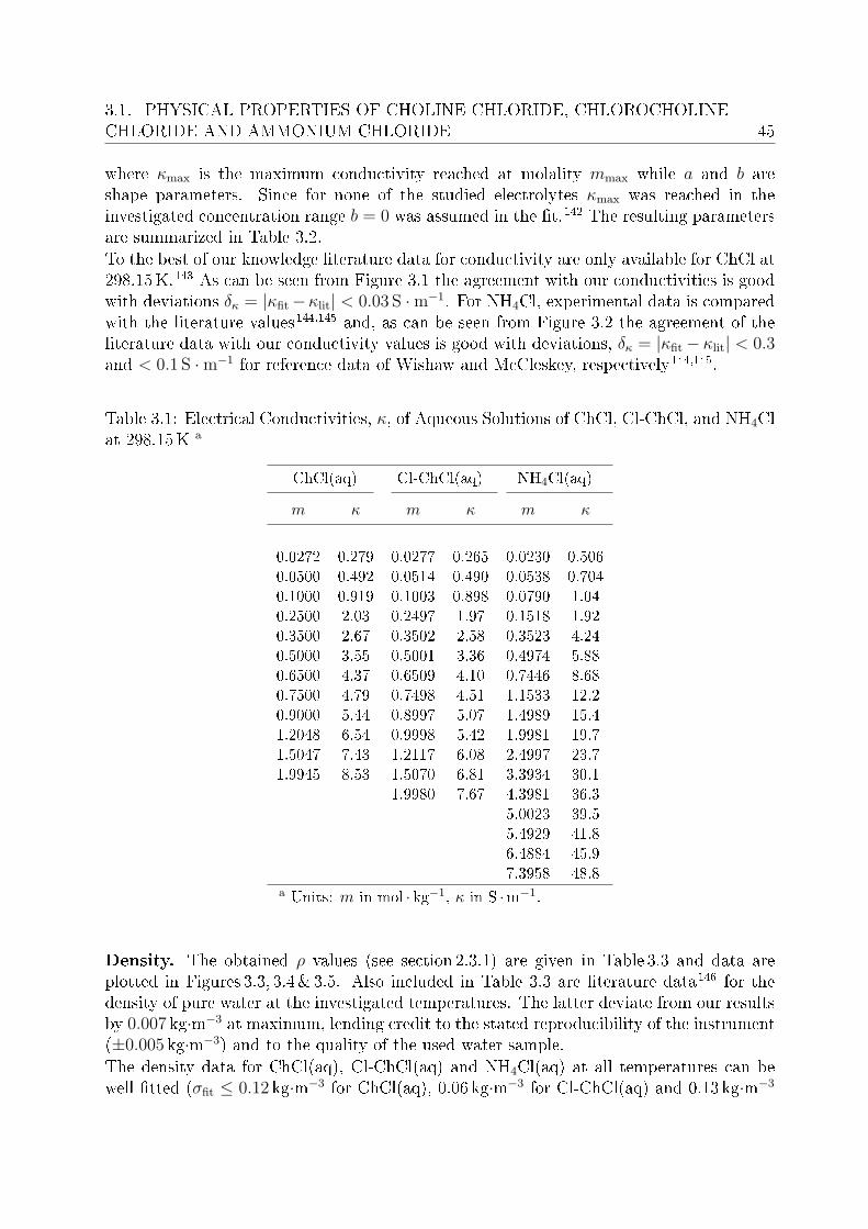
3.1. PHYSICAL PROPERTIES OF CHOLINE CHLORIDE, CHLOROCHOLINECHLORIDE AND AMMONIUM CHLORIDE 45
where κmax is the maximum conductivity reached at molality mmax while a and b areshape parameters. Since for none of the studied electrolytes κmax was reached in theinvestigated concentration range b = 0 was assumed in the t.142 The resulting parametersare summarized in Table 3.2.To the best of our knowledge literature data for conductivity are only available for ChCl at298.15K.143 As can be seen from Figure 3.1 the agreement with our conductivities is goodwith deviations δκ = |κfit−κlit| < 0.03 S ·m−1. For NH4Cl, experimental data is comparedwith the literature values144,145 and, as can be seen from Figure 3.2 the agreement of theliterature data with our conductivity values is good with deviations, δκ = |κfit − κlit| < 0.3and < 0.1 S ·m−1 for reference data of Wishaw and McCleskey, respectively144,145.
Table 3.1: Electrical Conductivities, κ, of Aqueous Solutions of ChCl, Cl-ChCl, and NH4Clat 298.15K a
ChCl(aq) Cl-ChCl(aq) NH4Cl(aq)
m κ m κ m κ
0.0272 0.279 0.0277 0.265 0.0230 0.5060.0500 0.492 0.0514 0.490 0.0538 0.7040.1000 0.919 0.1003 0.898 0.0790 1.040.2500 2.03 0.2497 1.97 0.1518 1.920.3500 2.67 0.3502 2.58 0.3523 4.240.5000 3.55 0.5001 3.36 0.4974 5.880.6500 4.37 0.6509 4.10 0.7446 8.680.7500 4.79 0.7498 4.51 1.1533 12.20.9000 5.44 0.8997 5.07 1.4989 15.41.2048 6.54 0.9998 5.42 1.9981 19.71.5047 7.43 1.2117 6.08 2.4997 23.71.9945 8.53 1.5070 6.81 3.3934 30.1
1.9980 7.67 4.3981 36.35.0023 39.55.4929 41.86.4884 45.97.3958 48.8
a Units: m in mol · kg−1, κ in S ·m−1.
Density. The obtained ρ values (see section 2.3.1) are given in Table 3.3 and data areplotted in Figures 3.3, 3.4& 3.5. Also included in Table 3.3 are literature data146 for thedensity of pure water at the investigated temperatures. The latter deviate from our resultsby 0.007 kg·m−3 at maximum, lending credit to the stated reproducibility of the instrument(±0.005 kg·m−3) and to the quality of the used water sample.The density data for ChCl(aq), Cl-ChCl(aq) and NH4Cl(aq) at all temperatures can bewell tted (σfit ≤ 0.12 kg·m−3 for ChCl(aq), 0.06 kg·m−3 for Cl-ChCl(aq) and 0.13 kg·m−3

46 CHAPTER 3. INVESTIGATION OF ELECTROLYTE SOLUTIONS
0.0 0.5 1.0 1.5 2.00
2
4
6
8
10
/ S
m-1
m / mol kg-1
Figure 3.1: Electrical conductivities, κ, of aqueous solutions of ChCl (N, this work; ⊕,Reference 143) and Cl-ChCl ( ) at 298.15K as a function of solute molality, m. Solid linesrepresent ts with the Casteel-Amis equation, Eq. 3.1.
0 1 2 3 4 5 6 7 80
10
20
30
40
50
/ S
m-1
m / mol kg-1
Figure 3.2: Electrical conductivities, κ, of aqueous solutions of NH4Cl(aq) as a functionof molality, m from this work (), Reference 144 ( ), and Reference 145 (N), at 25 C.Solid line represents t of Eq. 3.1.
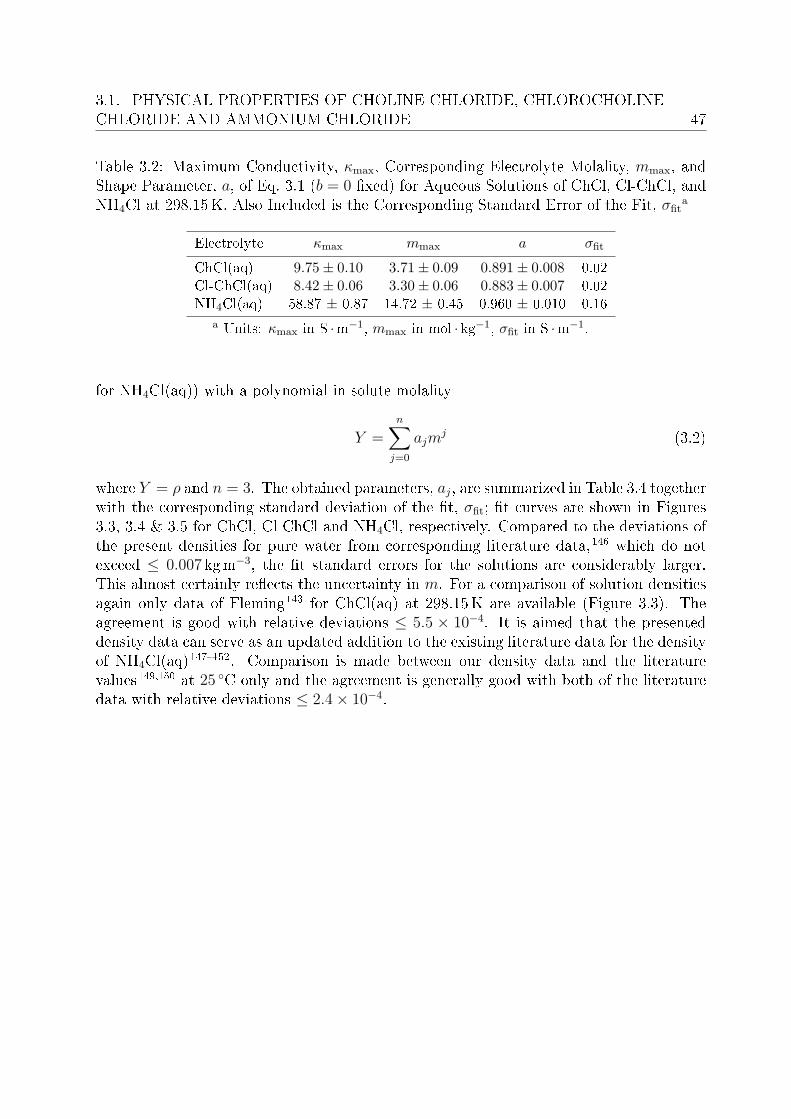
3.1. PHYSICAL PROPERTIES OF CHOLINE CHLORIDE, CHLOROCHOLINECHLORIDE AND AMMONIUM CHLORIDE 47
Table 3.2: Maximum Conductivity, κmax, Corresponding Electrolyte Molality, mmax, andShape Parameter, a, of Eq. 3.1 (b = 0 xed) for Aqueous Solutions of ChCl, Cl-ChCl, andNH4Cl at 298.15K. Also Included is the Corresponding Standard Error of the Fit, σfit
a
Electrolyte κmax mmax a σfit
ChCl(aq) 9.75± 0.10 3.71± 0.09 0.891± 0.008 0.02Cl-ChCl(aq) 8.42± 0.06 3.30± 0.06 0.883± 0.007 0.02NH4Cl(aq) 58.87 ± 0.87 14.72 ± 0.45 0.960 ± 0.010 0.16
a Units: κmax in S ·m−1, mmax in mol · kg−1, σfit in S ·m−1.
for NH4Cl(aq)) with a polynomial in solute molality
Y =n∑
j=0
ajmj (3.2)
where Y = ρ and n = 3. The obtained parameters, aj, are summarized in Table 3.4 togetherwith the corresponding standard deviation of the t, σfit; t curves are shown in Figures3.3, 3.4 & 3.5 for ChCl, Cl-ChCl and NH4Cl, respectively. Compared to the deviations ofthe present densities for pure water from corresponding literature data,146 which do notexceed ≤ 0.007 kgm−3, the t standard errors for the solutions are considerably larger.This almost certainly reects the uncertainty in m. For a comparison of solution densitiesagain only data of Fleming143 for ChCl(aq) at 298.15K are available (Figure 3.3). Theagreement is good with relative deviations ≤ 5.5 × 10⁻⁴. It is aimed that the presenteddensity data can serve as an updated addition to the existing literature data for the densityof NH4Cl(aq)147152. Comparison is made between our density data and the literaturevalues149,150 at 25 C only and the agreement is generally good with both of the literaturedata with relative deviations ≤ 2.4× 10⁻⁴.
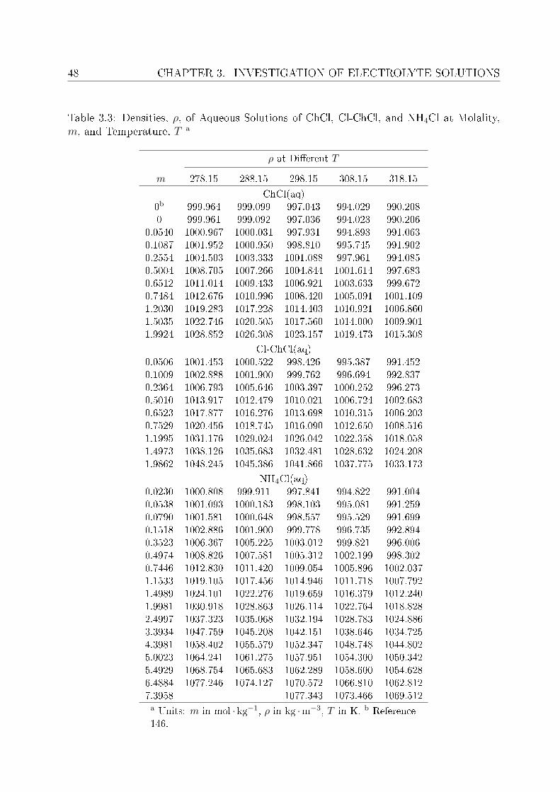
48 CHAPTER 3. INVESTIGATION OF ELECTROLYTE SOLUTIONS
Table 3.3: Densities, ρ, of Aqueous Solutions of ChCl, Cl-ChCl, and NH4Cl at Molality,m, and Temperature, T a
ρ at Dierent T
m 278.15 288.15 298.15 308.15 318.15
ChCl(aq)0b 999.964 999.099 997.043 994.029 990.2080 999.961 999.092 997.036 994.023 990.206
0.0540 1000.967 1000.031 997.931 994.893 991.0630.1087 1001.952 1000.950 998.810 995.745 991.9020.2554 1004.503 1003.333 1001.088 997.961 994.0850.5004 1008.705 1007.266 1004.844 1001.614 997.6830.6512 1011.014 1009.433 1006.921 1003.633 999.6720.7484 1012.676 1010.996 1008.420 1005.091 1001.1091.2030 1019.283 1017.228 1014.403 1010.921 1006.8601.5035 1022.746 1020.505 1017.560 1014.000 1009.9011.9924 1028.852 1026.308 1023.157 1019.473 1015.308
Cl-ChCl(aq)0.0506 1001.453 1000.522 998.426 995.387 991.4520.1009 1002.888 1001.900 999.762 996.694 992.8370.2364 1006.793 1005.646 1003.397 1000.252 996.2730.5010 1013.917 1012.479 1010.021 1006.724 1002.6830.6523 1017.877 1016.276 1013.698 1010.315 1006.2030.7529 1020.456 1018.745 1016.090 1012.650 1008.5161.1995 1031.176 1029.024 1026.042 1022.358 1018.0581.4973 1038.126 1035.683 1032.481 1028.632 1024.2081.9862 1048.245 1045.386 1041.866 1037.775 1033.173
NH4Cl(aq)0.0230 1000.808 999.911 997.841 994.822 991.0040.0538 1001.093 1000.183 998.103 995.081 991.2590.0790 1001.581 1000.648 998.557 995.529 991.6990.1518 1002.886 1001.900 999.778 996.735 992.8940.3523 1006.367 1005.225 1003.012 999.821 996.0060.4974 1008.826 1007.581 1005.312 1002.199 998.3020.7446 1012.830 1011.420 1009.054 1005.896 1002.0371.1533 1019.105 1017.456 1014.946 1011.718 1007.7921.4989 1024.101 1022.276 1019.659 1016.379 1012.2401.9981 1030.918 1028.863 1026.114 1022.764 1018.8282.4997 1037.323 1035.068 1032.194 1028.783 1024.8863.3934 1047.759 1045.208 1042.151 1038.646 1034.7254.3981 1058.402 1055.579 1052.347 1048.748 1044.8025.0023 1064.241 1061.275 1057.951 1054.300 1050.3425.4929 1068.754 1065.683 1062.289 1058.600 1054.6286.4884 1077.246 1074.127 1070.572 1066.810 1062.8127.3958 1077.343 1073.466 1069.512a Units: m in mol · kg−1, ρ in kg ·m−3, T in K. b Reference146.

3.1. PHYSICAL PROPERTIES OF CHOLINE CHLORIDE, CHLOROCHOLINECHLORIDE AND AMMONIUM CHLORIDE 49
0.0 0.5 1.0 1.5 2.0
990
995
1000
1005
1010
1015
1020
1025
1030
1035
/ kg
m-3
m / mol kg-1
Figure 3.3: Densities, ρ, of aqueous ChCl as a function of solute molality, m, at (,278.15; , 288.15; N, 298.15; H, 308.15 and J, 318.15)K. Solid lines represent ts ofEq. 3.2 (Y = ρ; n = 3). For comparison the data (⊕) of Fleming143 at 298.15K areincluded.
0.0 0.5 1.0 1.5 2.0
990
1000
1010
1020
1030
1040
1050
/ kg
m-3
m / mol kg-1
Figure 3.4: Densities, ρ, of aqueous solutions of Cl-ChCl as a function of solute molality,m, at (, 278.15; , 288.15; N, 298.15; H, 308.15 and J, 318.15)K. Solid lines representts of Eq. 3.2 (Y = ρ; n = 3).

50 CHAPTER 3. INVESTIGATION OF ELECTROLYTE SOLUTIONS
0 1 2 3 4 5 6 7 8980
1000
1020
1040
1060
1080
/ kg
m-3
m / mol kg-1
Figure 3.5: Densities, ρ, of aqueous solutions of NH4Cl(aq) as a function of solute molality,m, at (, 278.15; , 288.15; N, 298.15; H, 308.15 and J, 318.15)K. The data of References149 (), and 150 () are also given for comparison. Solid lines represent t of Eq. 3.2(Y = ρ; n = 3).
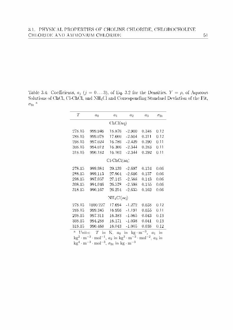
3.1. PHYSICAL PROPERTIES OF CHOLINE CHLORIDE, CHLOROCHOLINECHLORIDE AND AMMONIUM CHLORIDE 51
Table 3.4: Coecients, aj (j = 0 . . . 3), of Eq. 3.2 for the Densities, Y = ρ, of AqueousSolutions of ChCl, Cl-ChCl, and NH4Cl and Corresponding Standard Deviation of the Fit,σfit
a
T a0 a1 a2 a3 σfit
ChCl(aq)
278.15 999.946 18.876 -2.900 0.348 0.12288.15 999.078 17.600 -2.604 0.311 0.12298.15 997.024 16.786 -2.429 0.290 0.11308.15 994.012 16.306 -2.344 0.283 0.11318.15 990.182 16.103 -2.344 0.292 0.11
Cl-ChCl(aq)
278.15 999.984 29.139 -2.697 0.134 0.06288.15 999.113 27.964 -2.616 0.137 0.06298.15 997.057 27.145 -2.588 0.143 0.06308.15 994.046 26.578 -2.598 0.155 0.06318.15 990.167 26.254 -2.635 0.162 0.06
NH4Cl(aq)
278.15 1000.227 17.694 -1.272 0.058 0.12288.15 999.345 16.956 -1.191 0.055 0.11298.15 997.311 16.383 -1.065 0.043 0.13308.15 994.288 16.171 -1.038 0.041 0.13318.15 990.468 16.043 -1.005 0.038 0.12a Units: T in K, a0 in kg ·m−3, a1 inkg2 ·m−3 ·mol−1, a2 in kg3 ·m−3 ·mol−2, a3 inkg4 ·m−3 ·mol−3, σfit in kg ·m−3
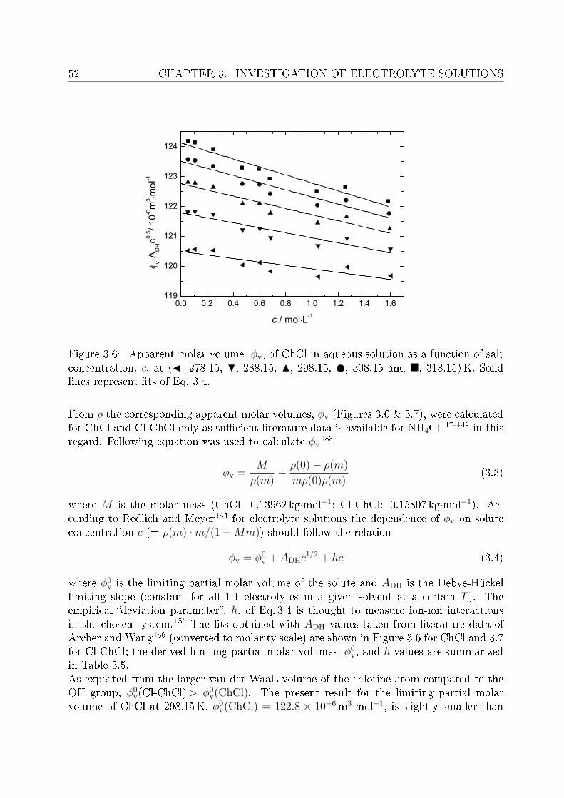
52 CHAPTER 3. INVESTIGATION OF ELECTROLYTE SOLUTIONS
0.0 0.2 0.4 0.6 0.8 1.0 1.2 1.4 1.6119
120
121
122
123
124
v-AD
Hc0.
5 / 10-6
m3
mol
-1
c / mol L-1
Figure 3.6: Apparent molar volume, ϕv, of ChCl in aqueous solution as a function of saltconcentration, c, at (J, 278.15; H, 288.15; N, 298.15; , 308.15 and , 318.15)K. Solidlines represent ts of Eq. 3.4.
From ρ the corresponding apparent molar volumes, ϕv (Figures 3.6 & 3.7), were calculatedfor ChCl and Cl-ChCl only as sucient literature data is available for NH4Cl147149 in thisregard. Following equation was used to calculate ϕv
153
ϕv =M
ρ(m)+
ρ(0)− ρ(m)
mρ(0)ρ(m)(3.3)
where M is the molar mass (ChCl: 0.13962 kg·mol−1; Cl-ChCl: 0.15807 kg·mol−1). Ac-cording to Redlich and Meyer154 for electrolyte solutions the dependence of ϕv on soluteconcentration c (= ρ(m) ·m/(1 +Mm)) should follow the relation
ϕv = ϕ0v + ADHc
1/2 + hc (3.4)
where ϕ0v is the limiting partial molar volume of the solute and ADH is the Debye-Hückel
limiting slope (constant for all 1:1 electrolytes in a given solvent at a certain T ). Theempirical deviation parameter, h, of Eq. 3.4 is thought to measure ion-ion interactionsin the chosen system.155 The ts obtained with ADH values taken from literature data ofArcher and Wang156 (converted to molarity scale) are shown in Figure 3.6 for ChCl and 3.7for Cl-ChCl; the derived limiting partial molar volumes, ϕ0
v, and h values are summarizedin Table 3.5.As expected from the larger van der Waals volume of the chlorine atom compared to theOH group, ϕ0
v(Cl-ChCl)> ϕ0v(ChCl). The present result for the limiting partial molar
volume of ChCl at 298.15K, ϕ0v(ChCl) = 122.8 × 10⁻⁶m3·mol−1, is slightly smaller than

3.1. PHYSICAL PROPERTIES OF CHOLINE CHLORIDE, CHLOROCHOLINECHLORIDE AND AMMONIUM CHLORIDE 53
0.0 0.2 0.4 0.6 0.8 1.0 1.2 1.4 1.6
126
127
128
129
130
131
132
v-AD
Hc0.
5 / 10-6
m3
mol
-1
c / mol L-1
Figure 3.7: Apparent molar volume, ϕv, of Cl-ChCl in aqueous solution as a function ofsalt concentration, c, at (J, 278.15; H, 288.15; N, 298.15; , 308.15 and , 318.15)K.Solid lines represent ts of Eq. 3.4.
the value published by Fleming143 (124.9 × 10⁻⁶m3·mol−1). This is mainly due to theslightly smaller densities of Reference 143 but the dierent ADH parameters used therealso contribute to the dierence.For ChCl and Cl-ChCl ϕ0
v increases with increasing temperature according to the relation
ϕ0v = aϕ0 + aϕ1(T − T0) + aϕ2(T − T0)
2 (3.5)
where T0 = 298.15K.157 The obtained parameters, aj (j = 0, . . . , 2), collected in Table 3.6,permit calculation of the limiting apparent molar expansibility
ϕ0E = (
∂ϕ0v
∂T)p = aϕ1 + 2aϕ2(T − T0) (3.6)
of ChCl and Cl-ChCl in water (Table 3.5) and of the corresponding Hepler's constant,158
(∂2ϕ0v/∂T
2)p = 2aϕ2 (= (−0.0023 ± 0.0002) × 10−6m3mol−1K−2 for ChCl; (−0.0013 ±0.0004)× 10−6m3mol−1K−2 for Cl-ChCl).Similar to aqueous NaCl solutions159 the deviation parameter, h, is negative and decreaseswith rising temperature for both ChCl(aq) and Cl-ChCl(aq). This suggests that ion-pairingis weak and ion-ion interactions decrease further with increasing thermal motions.159 Therather small concentration dependence of ϕ0
v (and thus small |h| values) for ChCl suggeststhat both ions well t into the water structure, whereas the fairly negative h for Cl-ChClmay indicate mutual salting-in of the ions, as discussed by Desnoyers and Arel for somen-alkylamine hydrobromides.153
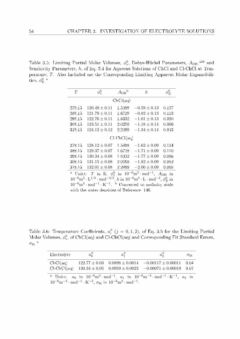
54 CHAPTER 3. INVESTIGATION OF ELECTROLYTE SOLUTIONS
Table 3.5: Limiting Partial Molar Volumes, ϕ0v, Debye-Hückel Parameters, ADH,156 and
Sensitivity Parameters, h, of Eq. 3.4 for Aqueous Solutions of ChCl and Cl-ChCl at Tem-perature, T . Also Included are the Corresponding Limiting Apparent Molar Expansibili-ties, ϕ0
Ea
T ϕ0v ADH
b h ϕ0E
ChCl(aq)
278.15 120.49± 0.11 1.5498 −0.59± 0.13 0.137288.15 121.79± 0.11 1.6728 −0.82± 0.13 0.113298.15 122.76± 0.11 1.8332 −1.01± 0.13 0.090308.15 123.51± 0.11 2.0259 −1.18± 0.14 0.066318.15 124.12± 0.12 2.2499 −1.34± 0.14 0.043
Cl-ChCl(aq)
278.15 128.12± 0.07 1.5498 −1.62± 0.09 0.124288.15 129.37± 0.07 1.6728 −1.71± 0.09 0.110298.15 130.34± 0.08 1.8332 −1.77± 0.09 0.096308.15 131.15± 0.08 2.0259 −1.82± 0.09 0.082318.15 132.01± 0.08 2.2499 −2.00± 0.09 0.068a Units: T in K, ϕ0
v in 10−6m3 ·mol−1, ADH in10−6m3 · L1/2 ·mol−3/2, h in 10−6m3 · L ·mol−2, ϕ0
E in10−6m3 ·mol−1 ·K−1. b Converted to molarity scalewith the water densities of Reference 146.
Table 3.6: Temperature Coecients, aϕi (j = 0, 1, 2), of Eq. 3.5 for the Limiting PartialMolar Volumes, ϕ0
v, of ChCl(aq) and Cl-ChCl(aq) and Corresponding Fit Standard Errors,σfit
a
Electrolyte aϕ0 aϕ1 aϕ2 σfit
ChCl(aq) 122.77± 0.03 0.0898± 0.0014 −0.00117± 0.00011 0.04Cl-ChCl(aq) 130.34± 0.05 0.0959± 0.0023 −0.00071± 0.00019 0.07
a Units: a0 in 10−6m3 ·mol−1, a1 in 10−6m−3 ·mol−1 ·K−1, a2 in10−6m−3 ·mol−1 ·K−2, σfit in 10−6m3 ·mol−1.

3.1. PHYSICAL PROPERTIES OF CHOLINE CHLORIDE, CHLOROCHOLINECHLORIDE AND AMMONIUM CHLORIDE 55
0.0 0.5 1.0 1.5 2.0
1
2
/ m
Pa
s
m / mol kg-1
Figure 3.8: Dynamic viscosities, η, of aqueous ChCl as a function of solute molality, m,at (, 278.15; , 288.15; N, 298.15; J, 308.15 and H, 318.15)K. Solid lines are the linearts of Eq. 3.2 (Y = η; n = 1). For comparison the data (⊕) of Fleming143 at 298.15K areincluded.
Viscosity. Dynamic viscosities, η, of aqueous solutions of ChCl (Figure 3.8), Cl-ChCl(Figure 3.9) and NH4Cl (Figure 3.10) were measured as a function of solute molality, m, atdierent temperatures, T . Dynamic viscosities determined for ChCl(aq) and Cl-ChCl(aq)are summarized in Table 3.7.∗ To the best of our knowledge only the data of Fleming143 forChCl(aq) at 298.15K are available for comparison (Figure 3.8). These are slightly largerthan the present results with relative deviations ≤ 3.4× 10⁻².For ChCl(aq) plots of η = f(m) are linear over the entire range ofm (Figure 3.8), whereas anotable curvature was found for Cl-ChCl(aq) (Figure 3.9). The data can be well-tted withEq. 3.2 where Y = η, n = 1 for ChCl, and n = 2 for Cl-ChCl. The obtained parametersare summarized in Table 3.8.
For liquids and solutions far from the glass-transition temperature, as should be the casefor the present samples, the temperature dependence of η is generally well-described bythe Arrhenius equation
ln η = ln η∞ + Ea/(RT ) (3.7)
where η∞ is the limiting viscosity for T → ∞, R the gas constant, and Ea the activationenergy of viscous ow.
∗Unfortunately, measured η data for NH4Cl were scattered (Figure 3.10) and none of the availablecapillaries was helpful to obtain reproducible set of viscosity data. Hence, data for NH4Cl are not shownin Table 3.7 and also further analysis for this system is not appropriate.

56 CHAPTER 3. INVESTIGATION OF ELECTROLYTE SOLUTIONS
0.0 0.5 1.0 1.5 2.00.5
1.0
1.5
2.0
2.5
/ m
Pa
s
m / mol kg-1
Figure 3.9: Dynamic viscosities, η, of aqueous Cl-ChCl as a function of solute molality,m, at (, 278.15; , 288.15; N, 298.15; J, 308.15 and H, 318.15)K. Solid lines are the tsof Eq. 3.2 (Y = η; n = 2).
0 1 2 3 4 5
0.885
0.890
0.895
0.900
0.905
0.910
0.915
0.920
/ m
Pa
s
m / mol kg-1
Figure 3.10: Dynamic viscosities, η, of aqueous NH4Cl as a function of solute molality, m,at 278.15K.

3.1. PHYSICAL PROPERTIES OF CHOLINE CHLORIDE, CHLOROCHOLINECHLORIDE AND AMMONIUM CHLORIDE 57
Table 3.7: Dynamic Viscosities, η, of Aqueous Solutions of ChCl and Cl-ChCl at Molality,m, and Temperature, T a
η at Dierent T
m 278.15 288.15 298.15 308.15 318.15
ChCl(aq)
0.0293 1.527 1.151 0.875 0.715 0.6330.0580 1.551 1.170 0.888 0.724 0.6100.1113 1.515 1.164 0.903 0.732 0.6230.2495 1.577 1.192 0.908 0.746 0.6380.3505 1.601 1.211 0.928 0.757 0.6460.4956 1.631 1.237 0.950 0.774 0.6560.6473 1.695 1.287 0.984 0.811 0.6940.7512 1.741 1.323 1.009 0.826 0.6900.9030 1.762 1.342 1.023 0.835 0.7021.0049 1.791 1.364 1.043 0.854 0.7211.2029 1.862 1.417 1.082 0.884 0.7471.5060 1.936 1.476 1.127 0.921 0.7761.9896 2.077 1.587 1.234 1.007 0.843
Cl-ChCl(aq)
0.0236 1.526 1.148 0.907 0.711 0.5960.0464 1.536 1.156 0.913 0.714 0.5950.0994 1.555 1.172 0.924 0.722 0.6020.2464 1.610 1.211 0.955 0.757 0.6450.3552 1.656 1.241 0.977 0.770 0.6600.4990 1.712 1.286 1.012 0.793 0.6610.6479 1.778 1.335 1.047 0.831 0.6940.7493 1.815 1.362 1.069 0.833 0.6910.9041 1.914 1.433 1.124 0.879 0.7330.9927 1.933 1.447 1.133 0.890 0.7501.1758 2.010 1.502 1.173 0.915 0.7591.5415 2.298 1.708 1.292 1.005 0.8352.1484 2.612 1.932 1.493 1.158 0.948
a Units: m in mol · kg−1, η in mPa · s, T in K.
Figure 3.11 shows the activation energies obtained from the present viscosity data alongwith the calculated Ea value of pure water using literature data160. For ChCl(aq) Ea isessentially independent of solute molality over the entire concentration range, yielding anaverage value of 16.9 kJ·mol−1, whereas Ea appears to increase linearly for Cl-ChCl(aq).However, these results have to be taken with a grain of salt. Error bars for Ea are ratherlarge, and a close inspection of the ts (Figures 3.12 & 3.13) reveals that especially at low
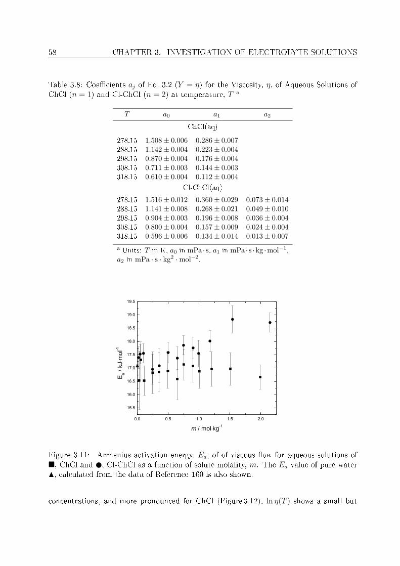
58 CHAPTER 3. INVESTIGATION OF ELECTROLYTE SOLUTIONS
Table 3.8: Coecients aj of Eq. 3.2 (Y = η) for the Viscosity, η, of Aqueous Solutions ofChCl (n = 1) and Cl-ChCl (n = 2) at temperature, T a
T a0 a1 a2
ChCl(aq)
278.15 1.508± 0.006 0.286± 0.007288.15 1.142± 0.004 0.223± 0.004298.15 0.870± 0.004 0.176± 0.004308.15 0.711± 0.003 0.144± 0.003318.15 0.610± 0.004 0.112± 0.004
Cl-ChCl(aq)
278.15 1.516± 0.012 0.360± 0.029 0.073± 0.014288.15 1.141± 0.008 0.268± 0.021 0.049± 0.010298.15 0.904± 0.003 0.196± 0.008 0.036± 0.004308.15 0.800± 0.004 0.157± 0.009 0.024± 0.004318.15 0.596± 0.006 0.134± 0.014 0.013± 0.007
a Units: T in K, a0 in mPa · s, a1 in mPa · s ·kg ·mol−1,a2 in mPa · s · kg2 ·mol−2.
0.0 0.5 1.0 1.5 2.0
15.5
16.0
16.5
17.0
17.5
18.0
18.5
19.0
19.5
Ea /
kJm
ol-1
m / mol kg-1
Figure 3.11: Arrhenius activation energy, Ea, of of viscous ow for aqueous solutions of, ChCl and , Cl-ChCl as a function of solute molality, m. The Ea value of pure waterN, calculated from the data of Reference 160 is also shown.
concentrations, and more pronounced for ChCl (Figure 3.12), ln η(T ) shows a small but
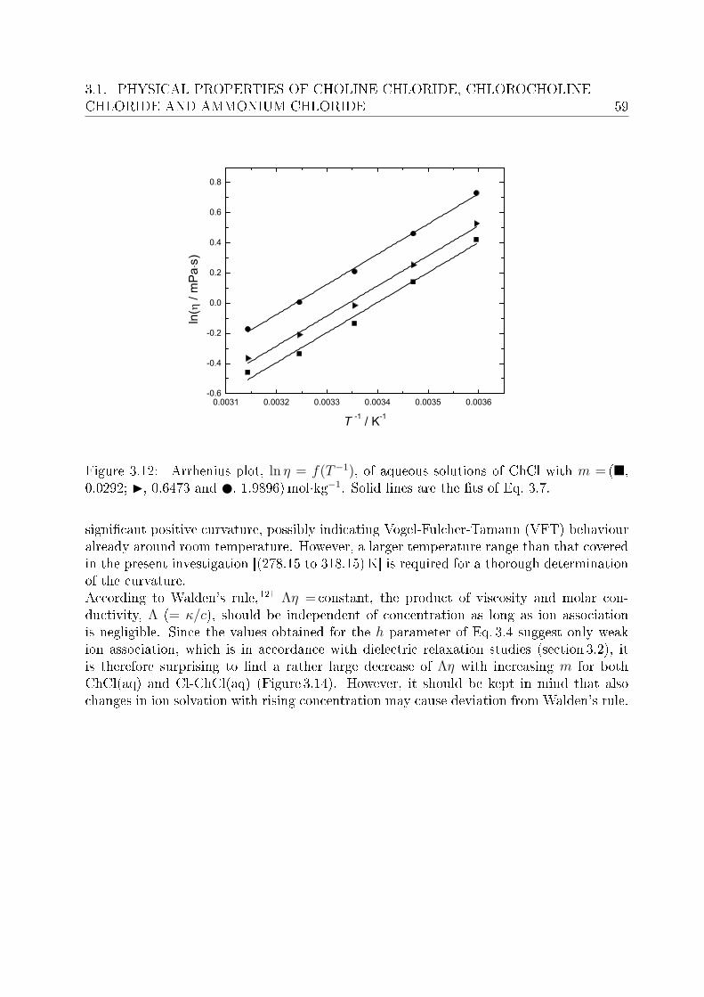
3.1. PHYSICAL PROPERTIES OF CHOLINE CHLORIDE, CHLOROCHOLINECHLORIDE AND AMMONIUM CHLORIDE 59
0.0031 0.0032 0.0033 0.0034 0.0035 0.0036-0.6
-0.4
-0.2
0.0
0.2
0.4
0.6
0.8
ln(
/ m
Pa
s)
T -1 / K-1
Figure 3.12: Arrhenius plot, ln η = f(T−1), of aqueous solutions of ChCl with m = (,0.0292; I, 0.6473 and , 1.9896)mol·kg−1. Solid lines are the ts of Eq. 3.7.
signicant positive curvature, possibly indicating Vogel-Fulcher-Tamann (VFT) behaviouralready around room temperature. However, a larger temperature range than that coveredin the present investigation [(278.15 to 318.15)K] is required for a thorough determinationof the curvature.According to Walden's rule,121 Λη = constant, the product of viscosity and molar con-ductivity, Λ (= κ/c), should be independent of concentration as long as ion associationis negligible. Since the values obtained for the h parameter of Eq. 3.4 suggest only weakion association, which is in accordance with dielectric relaxation studies (section 3.2), itis therefore surprising to nd a rather large decrease of Λη with increasing m for bothChCl(aq) and Cl-ChCl(aq) (Figure 3.14). However, it should be kept in mind that alsochanges in ion solvation with rising concentration may cause deviation from Walden's rule.

60 CHAPTER 3. INVESTIGATION OF ELECTROLYTE SOLUTIONS
0.0031 0.0032 0.0033 0.0034 0.0035 0.0036-0.6
-0.4
-0.2
0.0
0.2
0.4
0.6
0.8
1.0
ln(
/ m
Pa
s)
T -1 / K-1
Figure 3.13: Arrhenius plot, ln η = f(T−1), of aqueous solutions of Cl-ChCl with m = (,0.0236; I, 0.6479 and , 2.1484)mol·kg−1. Solid lines are the ts of Eq. 3.7.
0.0 0.2 0.4 0.6 0.8 1.0 1.2 1.4 1.66.0
6.5
7.0
7.5
8.0
8.5
9.0
/103 S
m2
mol
-1P
as
c / mol L-1
Figure 3.14: Walden product, Λη, of aqueous solutions of H, ChCl and , Cl-ChCl at298.15K.

3.2. DRS OF CHOLINE CHLORIDE, CHLOROCHOLINE CHLORIDE ANDAMMONIUM CHLORIDE 61
3.2 DRS of choline chloride, chlorocholine chloride and
ammonium chloride
Most of the material presented in this section makes the basis of the manuscript:
Shaukat, S.; Buchner, R. `Dielectric Relaxation Spectroscopy of Hydration and Ion-pairingin Aqueous Solutions of Choline Chloride, Chlorocholine Chloride, and Ammonium Chlo-ride.' Phys. Chem. Chem. Phy, In preparation.
The present section deals with broadband DRS study of aqueous solution of ammoniumchloride, choline chloride and chloro-chlone chloride. DR spectra were measured over thefrequency range of ∼0.2 GHz to 89 GHz upto fairly high concentrations at 25 C. Addi-tionally, spectra of 0.280mol · kg−1 of ChCl(aq) were measured at 5, 15, 25, 35, 45, 55 and65 C.The data in the frequency range 0.2 ≤ ν/GHz ≤ 50 were recorded with Agilent E8364BVNA (section 2.2.3) and high frequency data, 60 ≤ ν/GHz ≤ 89 was recorded using E-bandinterferometer (section 2.2.2).
3.2.1 Choice of t model
The combined ε(ν) data were analyzed by simultaneously tting the in-phase (ε′(ν), Fig-ures 3.15a - 3.18a) and out-of-phase (ε′′(ν), Figures 3.15b & 3.18b) components of thecomplex permittivity to various relaxation models with n distinguishable relaxation pro-cesses using Eq. 1.66. Only simplied variants of Eq. 1.66, i.e., CD, CC, and D modelswere considered.21 The quality of the t was evaluated via χ2
r values.103 Along with theminimum variance, the choice of accepted model was also based on one oering least num-ber of modes which are physically explainable. All tting parameters obtained from thepresent spectra are summarized in Tables 3.9 and 3.10.The method devised by Zasetzky and Buchner105 was used additionally to check the validityof accepted model for each of the studied salt. Typical results of that analysis are shownin Figure 3.19.
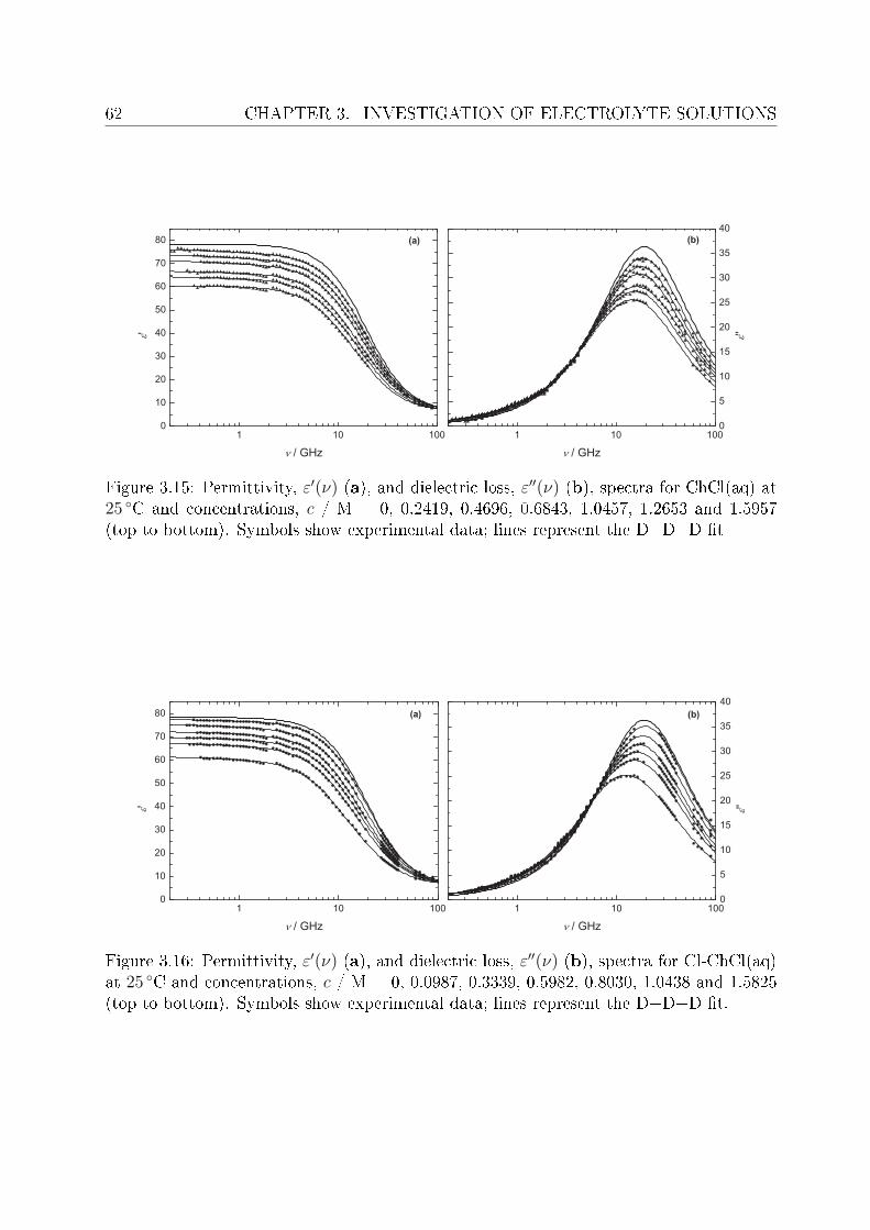
62 CHAPTER 3. INVESTIGATION OF ELECTROLYTE SOLUTIONS
Figure 3.15: Permittivity, ε′(ν) (a), and dielectric loss, ε′′(ν) (b), spectra for ChCl(aq) at25 C and concentrations, c / M = 0, 0.2419, 0.4696, 0.6843, 1.0457, 1.2653 and 1.5957(top to bottom). Symbols show experimental data; lines represent the D+D+D t
Figure 3.16: Permittivity, ε′(ν) (a), and dielectric loss, ε′′(ν) (b), spectra for Cl-ChCl(aq)at 25 C and concentrations, c / M = 0, 0.0987, 0.3339, 0.5982, 0.8030, 1.0438 and 1.5825(top to bottom). Symbols show experimental data; lines represent the D+D+D t.
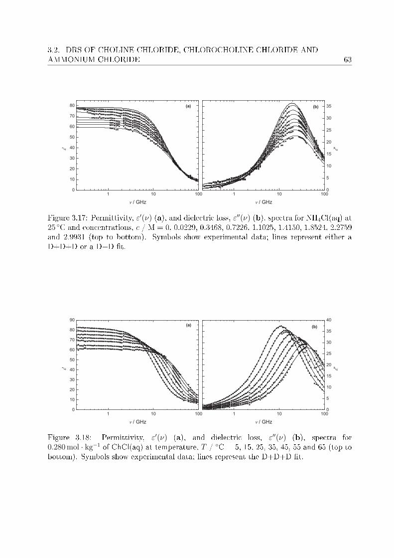
3.2. DRS OF CHOLINE CHLORIDE, CHLOROCHOLINE CHLORIDE ANDAMMONIUM CHLORIDE 63
Figure 3.17: Permittivity, ε′(ν) (a), and dielectric loss, ε′′(ν) (b), spectra for NH4Cl(aq) at25 C and concentrations, c / M = 0, 0.0229, 0.3468, 0.7226, 1.1025, 1.4150, 1.8524, 2.2759and 2.9931 (top to bottom). Symbols show experimental data; lines represent either aD+D+D or a D+D t.
Figure 3.18: Permittivity, ε′(ν) (a), and dielectric loss, ε′′(ν) (b), spectra for0.280mol · kg−1 of ChCl(aq) at temperature, T / C = 5, 15, 25, 35, 45, 55 and 65 (top tobottom). Symbols show experimental data; lines represent the D+D+D t.
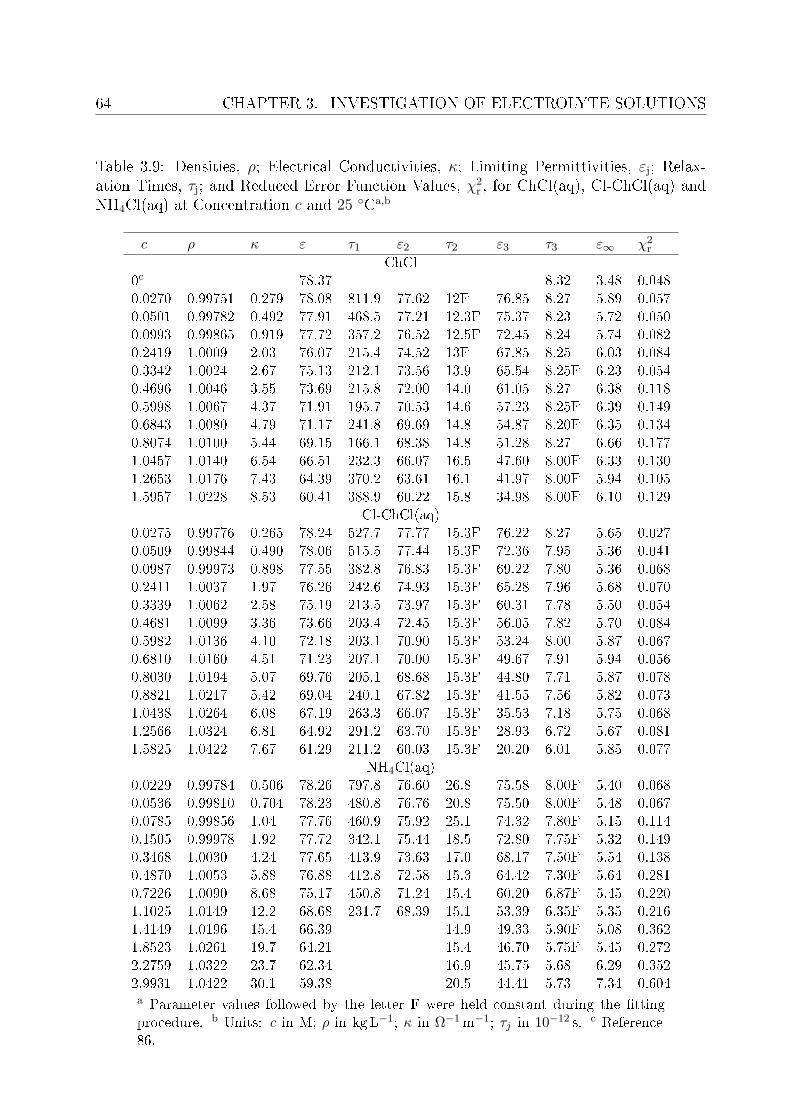
64 CHAPTER 3. INVESTIGATION OF ELECTROLYTE SOLUTIONS
Table 3.9: Densities, ρ; Electrical Conductivities, κ; Limiting Permittivities, εj; Relax-ation Times, τj; and Reduced Error Function Values, χ2
r , for ChCl(aq), Cl-ChCl(aq) andNH4Cl(aq) at Concentration c and 25 Ca,b
c ρ κ ε τ1 ε2 τ2 ε3 τ3 ε∞ χ2r
ChCl0c 78.37 8.32 3.48 0.0480.0270 0.99751 0.279 78.08 811.9 77.62 12F 76.85 8.27 5.89 0.0570.0501 0.99782 0.492 77.91 468.5 77.21 12.3F 75.37 8.23 5.72 0.0500.0993 0.99865 0.919 77.72 357.2 76.52 12.5F 72.45 8.24 5.74 0.0820.2419 1.0009 2.03 76.07 215.4 74.52 13F 67.85 8.25 6.03 0.0840.3342 1.0024 2.67 75.13 212.1 73.56 13.9 65.54 8.25F 6.23 0.0540.4696 1.0046 3.55 73.69 215.8 72.00 14.0 61.05 8.27 6.38 0.1180.5998 1.0067 4.37 71.91 195.7 70.53 14.6 57.23 8.25F 6.39 0.1490.6843 1.0080 4.79 71.17 241.8 69.69 14.8 54.87 8.20F 6.35 0.1340.8074 1.0100 5.44 69.15 166.1 68.38 14.8 51.28 8.27 6.66 0.1771.0457 1.0140 6.54 66.51 232.3 66.07 16.5 47.60 8.00F 6.33 0.1301.2653 1.0176 7.43 64.39 370.2 63.61 16.1 41.97 8.00F 5.94 0.1051.5957 1.0228 8.53 60.41 388.9 60.22 15.8 34.98 8.00F 6.10 0.129
Cl-ChCl(aq)0.0275 0.99776 0.265 78.24 527.7 77.77 15.3F 76.22 8.27 5.65 0.0270.0509 0.99844 0.490 78.06 515.5 77.44 15.3F 72.36 7.95 5.36 0.0410.0987 0.99973 0.898 77.55 382.8 76.83 15.3F 69.22 7.80 5.36 0.0680.2411 1.0037 1.97 76.26 242.6 74.93 15.3F 65.28 7.96 5.68 0.0700.3339 1.0062 2.58 75.19 213.5 73.97 15.3F 60.31 7.78 5.50 0.0540.4681 1.0099 3.36 73.66 203.4 72.45 15.3F 56.05 7.82 5.70 0.0840.5982 1.0136 4.10 72.18 203.1 70.90 15.3F 53.24 8.00 5.87 0.0670.6810 1.0160 4.51 71.23 207.1 70.00 15.3F 49.67 7.91 5.94 0.0560.8030 1.0194 5.07 69.76 205.1 68.68 15.3F 44.80 7.71 5.87 0.0780.8821 1.0217 5.42 69.04 240.1 67.82 15.3F 41.55 7.56 5.82 0.0731.0438 1.0264 6.08 67.19 263.3 66.07 15.3F 35.53 7.18 5.75 0.0681.2566 1.0324 6.81 64.92 291.2 63.70 15.3F 28.93 6.72 5.67 0.0811.5825 1.0422 7.67 61.29 211.2 60.03 15.3F 20.20 6.01 5.85 0.077
NH4Cl(aq)0.0229 0.99784 0.506 78.26 797.8 76.60 26.8 75.58 8.00F 5.40 0.0680.0536 0.99810 0.704 78.23 480.8 76.76 20.8 75.50 8.00F 5.48 0.0670.0785 0.99856 1.04 77.76 460.9 75.92 25.1 74.32 7.80F 5.15 0.1140.1505 0.99978 1.92 77.72 342.1 75.44 18.5 72.80 7.75F 5.32 0.1490.3468 1.0030 4.24 77.65 413.9 73.63 17.0 68.17 7.50F 5.54 0.1380.4870 1.0053 5.88 76.88 412.8 72.58 15.3 64.42 7.30F 5.64 0.2810.7226 1.0090 8.68 75.17 450.8 71.24 15.4 60.20 6.87F 5.45 0.2201.1025 1.0149 12.2 68.68 231.7 68.39 15.1 53.39 6.35F 5.35 0.2161.4149 1.0196 15.4 66.39 14.9 49.33 5.90F 5.08 0.3621.8523 1.0261 19.7 64.21 15.4 46.70 5.75F 5.45 0.2722.2759 1.0322 23.7 62.34 16.9 45.75 5.68 6.29 0.3522.9931 1.0422 30.1 59.38 20.5 44.41 5.73 7.34 0.604a Parameter values followed by the letter F were held constant during the ttingprocedure. b Units: c in M; ρ in kg L−1; κ in Ω−1m−1; τj in 10−12 s. c Reference86.
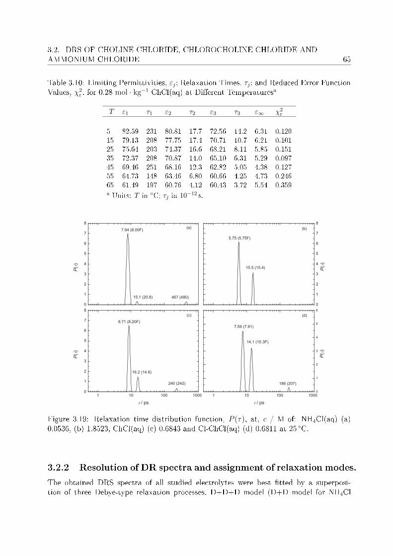
3.2. DRS OF CHOLINE CHLORIDE, CHLOROCHOLINE CHLORIDE ANDAMMONIUM CHLORIDE 65
Table 3.10: Limiting Permittivities, εj; Relaxation Times, τj; and Reduced Error FunctionValues, χ2
r , for 0.28 mol · kg−1 ChCl(aq) at Dierent Temperaturesa
T ε1 τ1 ε2 τ2 ε3 τ3 ε∞ χ2r
5 82.59 231 80.81 17.7 72.56 14.2 6.31 0.12015 79.13 208 77.75 17.4 70.71 10.7 6.21 0.10125 75.64 203 74.37 16.6 68.21 8.11 5.85 0.15135 72.37 208 70.87 14.0 65.10 6.31 5.29 0.09745 69.46 251 68.16 12.3 62.82 5.05 4.38 0.12755 64.73 148 63.46 6.80 60.66 4.25 4.73 0.24665 61.49 197 60.76 4.12 60.43 3.72 5.54 0.359a Units: T in C; τj in 10−12 s.
Figure 3.19: Relaxation time distribution function, P (τ), at, c / M of: NH4Cl(aq) (a)0.0536, (b) 1.8523, ChCl(aq) (c) 0.6843 and Cl-ChCl(aq) (d) 0.6811 at 25 C.
3.2.2 Resolution of DR spectra and assignment of relaxation modes.
The obtained DRS spectra of all studied electrolytes were best tted by a superposi-tion of three Debye-type relaxation processes, D+D+D model (D+D model for NH4Cl
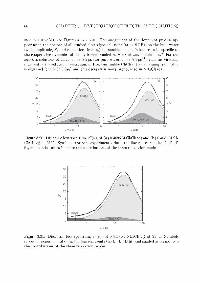
66 CHAPTER 3. INVESTIGATION OF ELECTROLYTE SOLUTIONS
at c > 1.1025M), see Figures 3.15 - 3.21. The assignment of the dominant process ap-pearing in the spectra of all studied electrolyte solutions (at ∼18GHz) to the bulk water(with amplitude, Sb and relaxation time, τb) is unambiguous, as is known to be specic tothe cooperative dynamics of the hydrogen-bonded network of water molecules.64 For theaqueous solutions of ChCl, τb ≈ 8.2ps (for pure water, τb ≈ 8.3 ps64), remains virtuallyinvariant of the solute concentration, c. However, unlike ChCl(aq) a decreasing trend of τbis observed for Cl-ChCl(aq) and this decrease is more pronounced in NH4Cl(aq).
Figure 3.20: Dielectric loss spectrum, ε′′(ν), of (a) 0.4696M ChCl(aq) and (b) 0.4681M Cl-ChCl(aq) at 25 C. Symbols represent experimental data, the line represents the D+D+Dt, and shaded areas indicate the contributions of the three relaxation modes
Figure 3.21: Dielectric loss spectrum, ε′′(ν), of 0.3468M NH4Cl(aq) at 25 C. Symbolsrepresent experimental data, the line represents the D+D+D t, and shaded areas indicatethe contributions of the three relaxation modes
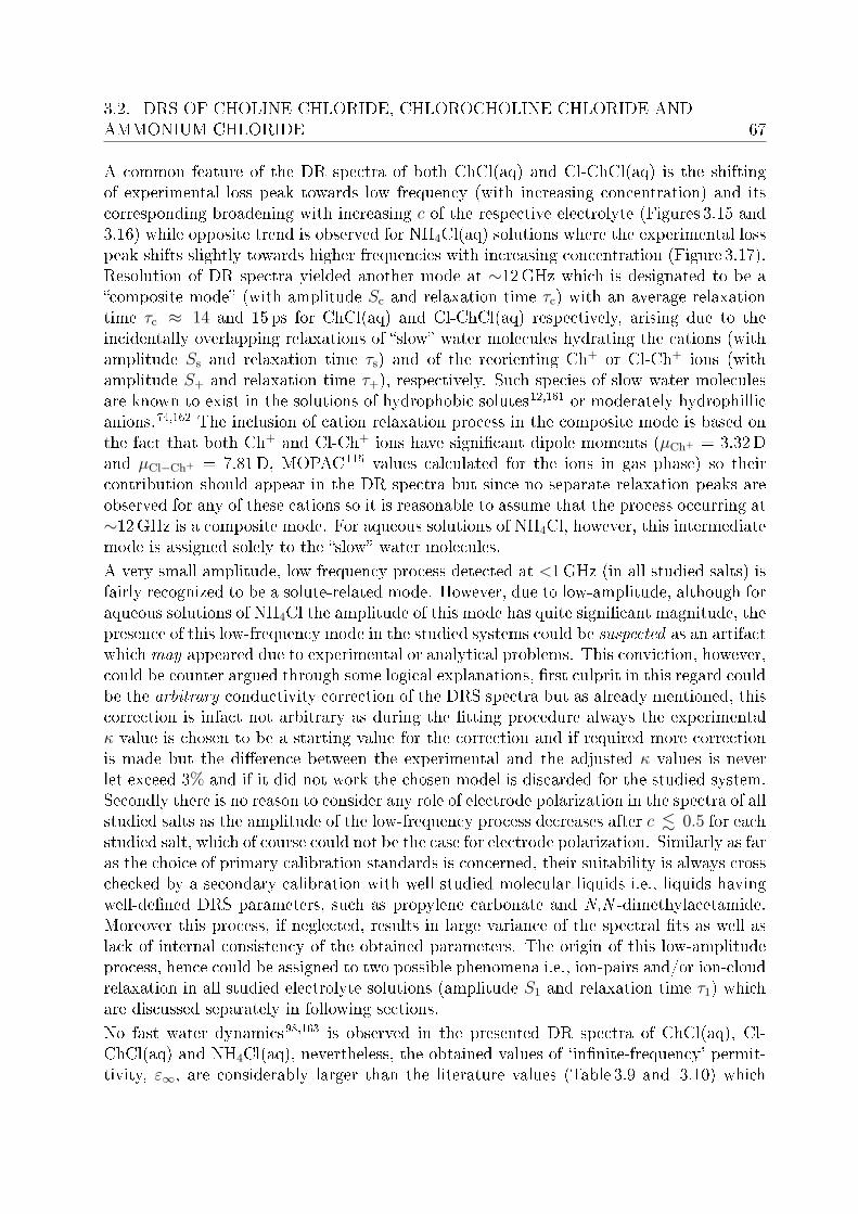
3.2. DRS OF CHOLINE CHLORIDE, CHLOROCHOLINE CHLORIDE ANDAMMONIUM CHLORIDE 67
A common feature of the DR spectra of both ChCl(aq) and Cl-ChCl(aq) is the shiftingof experimental loss peak towards low frequency (with increasing concentration) and itscorresponding broadening with increasing c of the respective electrolyte (Figures 3.15 and3.16) while opposite trend is observed for NH4Cl(aq) solutions where the experimental losspeak shifts slightly towards higher frequencies with increasing concentration (Figure 3.17).Resolution of DR spectra yielded another mode at ∼12GHz which is designated to be acomposite mode (with amplitude Sc and relaxation time τc) with an average relaxationtime τc ≈ 14 and 15 ps for ChCl(aq) and Cl-ChCl(aq) respectively, arising due to theincidentally overlapping relaxations of slow water molecules hydrating the cations (withamplitude Ss and relaxation time τs) and of the reorienting Ch+ or Cl-Ch+ ions (withamplitude S+ and relaxation time τ+), respectively. Such species of slow water moleculesare known to exist in the solutions of hydrophobic solutes12,161 or moderately hydrophillicanions.74,162 The inclusion of cation relaxation process in the composite mode is based onthe fact that both Ch+ and Cl-Ch+ ions have signicant dipole moments (µCh+ = 3.32Dand µCl−Ch+ = 7.81D, MOPAC115 values calculated for the ions in gas phase) so theircontribution should appear in the DR spectra but since no separate relaxation peaks areobserved for any of these cations so it is reasonable to assume that the process occurring at∼12GHz is a composite mode. For aqueous solutions of NH4Cl, however, this intermediatemode is assigned solely to the slow water molecules.A very small amplitude, low frequency process detected at <1GHz (in all studied salts) isfairly recognized to be a solute-related mode. However, due to low-amplitude, although foraqueous solutions of NH4Cl the amplitude of this mode has quite signicant magnitude, thepresence of this low-frequency mode in the studied systems could be suspected as an artifactwhich may appeared due to experimental or analytical problems. This conviction, however,could be counter argued through some logical explanations, rst culprit in this regard couldbe the arbitrary conductivity correction of the DRS spectra but as already mentioned, thiscorrection is infact not arbitrary as during the tting procedure always the experimentalκ value is chosen to be a starting value for the correction and if required more correctionis made but the dierence between the experimental and the adjusted κ values is neverlet exceed 3% and if it did not work the chosen model is discarded for the studied system.Secondly there is no reason to consider any role of electrode polarization in the spectra of allstudied salts as the amplitude of the low-frequency process decreases after c . 0.5 for eachstudied salt, which of course could not be the case for electrode polarization. Similarly as faras the choice of primary calibration standards is concerned, their suitability is always crosschecked by a secondary calibration with well studied molecular liquids i.e., liquids havingwell-dened DRS parameters, such as propylene carbonate and N,N -dimethylacetamide.Moreover this process, if neglected, results in large variance of the spectral ts as well aslack of internal consistency of the obtained parameters. The origin of this low-amplitudeprocess, hence could be assigned to two possible phenomena i.e., ion-pairs and/or ion-cloudrelaxation in all studied electrolyte solutions (amplitude S1 and relaxation time τ1) whichare discussed separately in following sections.No fast water dynamics98,163 is observed in the presented DR spectra of ChCl(aq), Cl-ChCl(aq) and NH4Cl(aq), nevertheless, the obtained values of `innite-frequency' permit-tivity, ε∞, are considerably larger than the literature values (Table 3.9 and 3.10) which
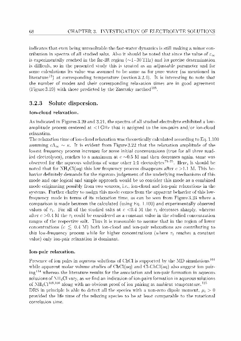
68 CHAPTER 3. INVESTIGATION OF ELECTROLYTE SOLUTIONS
indicates that even being unresolvable the fast-water dynamics is still making a minor con-tribution in spectra of all studied salts. Also it should be noted that since the value of ε∞is experimentally reached in the far-IR region (∼1 - 30THz) and its precise determinationis dicult, so in the presented study this is treated as an adjustable parameter and forsome calculations its value was assumed to be same as for pure water (as mentioned inliterature73) at corresponding temperature (section 3.2.4). It is interesting to note thatthe number of modes and their corresponding relaxation times are in good agreement(Figure 3.19) with those predicted by the Zasetsky method105.
3.2.3 Solute dispersion.
Ion-cloud relaxation.
As indicated in Figures 3.20 and 3.21, the spectra of all studied electrolyte exhibited a low-amplitude process centered at <1GHz that is assigned to the ion-pairs and/or ion-cloudrelaxation.The relaxation time of ion-cloud relaxation was theoretically calculated according to Eq. 1.100assuming cΛ∞ ∼ κ. It is evident from Figure 3.22 that the relaxation amplitude of thelowest frequency process increases for some initial concentrations (true for all three stud-ied electrolytes), reaches to a maximum at c ∼0.5 M and then decreases again, same wasobserved for the aqueous solutions of some other 1:1 electrolytes7375. Here, it should benoted that for NH4Cl(aq) this low frequency process disappears after c >1.1 M. This be-havior denitely demands for the rigorous judgement of the underlying mechanisms of thismode and one logical and simple approach would be to consider this mode as a combinedmode originating possibly from two sources, i.e., ion-cloud and ion-pair relaxations in thesystems. Further clarity to assign this mode comes from the apparent behavior of this low-frequency mode in terms of its relaxation time, as can be seen from Figure 3.23 where acomparison is made between the calculated (using Eq. 1.100) and experimentally observedvalues of τ1. For all of the studied salts at c <0.4 M the τ1 decreases sharply, whereasafter c >0.4 M the τ1 could be considered as a constant value in the studied concentrationranges of the respective salt. Thus it is reasonable to assume that in the region of lowerconcentrations (c . 0.4 M) both ion-cloud and ion-pair relaxations are contributing tothis low-frequency process while for higher concentrations (where τ1 reaches a constantvalue) only ion-pair relaxation is dominant.
Ion-pair relaxation.
Presence of ion pairs in aqueous solutions of ChCl is supported by the MD simulations164
while apparent molar volume studies of ChCl(aq) and Cl-ChCl(aq) also suggest ion pair-ing114 whereas the literature results for the association and ion-pair formation in aqueoussolutions of NH4Cl vary, as we nd an indication of ion-pairs formation in aqueous solutionsof NH4Cl165,166 along with no obvious proof of ion pairing at ambient temperature.125
DRS in principle is able to detect all the species with a non-zero dipole moment, µi > 0provided the life time of the relaxing species to be at least comparable to the rotationalcorrelation time.
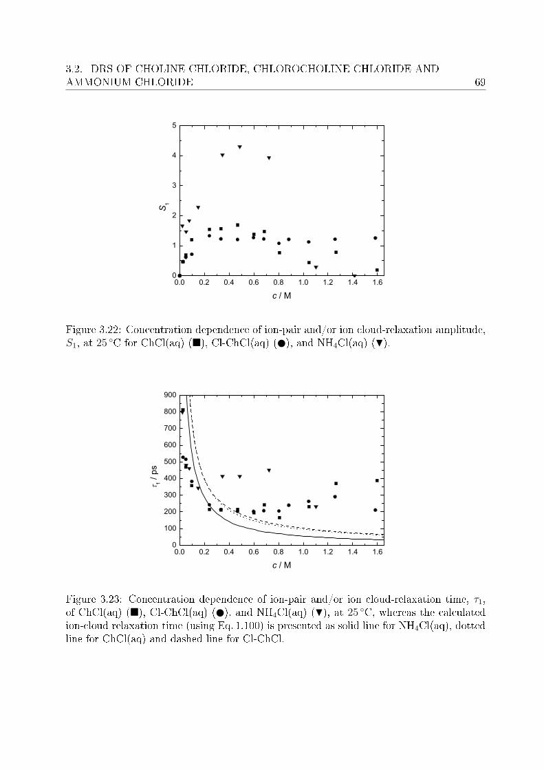
3.2. DRS OF CHOLINE CHLORIDE, CHLOROCHOLINE CHLORIDE ANDAMMONIUM CHLORIDE 69
0.0 0.2 0.4 0.6 0.8 1.0 1.2 1.4 1.60
1
2
3
4
5
S1
c / M
Figure 3.22: Concentration dependence of ion-pair and/or ion cloud-relaxation amplitude,S1, at 25 C for ChCl(aq) (), Cl-ChCl(aq) ( ), and NH4Cl(aq) (H).
0.0 0.2 0.4 0.6 0.8 1.0 1.2 1.4 1.60
100
200
300
400
500
600
700
800
900
1 / ps
c / M
Figure 3.23: Concentration dependence of ion-pair and/or ion cloud-relaxation time, τ1,of ChCl(aq) (), Cl-ChCl(aq) ( ), and NH4Cl(aq) (H), at 25 C, whereas the calculatedion-cloud relaxation time (using Eq. 1.100) is presented as solid line for NH4Cl(aq), dottedline for ChCl(aq) and dashed line for Cl-ChCl.
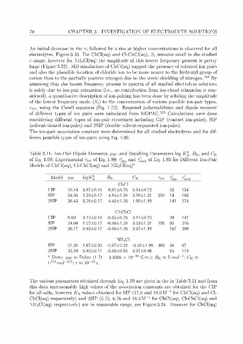
70 CHAPTER 3. INVESTIGATION OF ELECTROLYTE SOLUTIONS
An initial decrease in the τ1 followed by a rise at higher concentrations is observed for allelectrolytes, Figure 3.23. For ChCl(aq) and Cl-ChCl(aq), S1 remains small in the studiedc range, however for NH4Cl(aq) the amplitude of this lowest frequency process is prettylarge (Figure 3.22). MD simulations of ChCl(aq) suggest the presence of solvated ion pairsand also the plausible location of chloride ion to be more nearer to the hydroxyl group ofcation than to the partially positive nitrogen due to the steric shielding of nitrogen.164 Byassuming that the lowest frequency process in spectra of all studied electrolyte solutionsis solely due to ion-pair relaxation (i.e., no contribution from ion-cloud relaxation is con-sidered), a quantitative description of ion-pairing has been done by relating the amplitudeof the lowest frequency mode (S1) to the concentration of various possible ion-pair types,cIP , using the Cavell equation (Eq. 1.72). Required polarizabilities and dipole momentof dierent types of ion pairs were calculated from MOPAC.115 Calculations were doneconsidering dierent types of ion-pair structures including CIP (contact ion-pairs), SIP(solvent-shared ion-pairs) and 2SIP (double solvent-separated ion-pairs).The ion-pair association constant were determined for all studied electrolytes and for dif-ferent possible types of ion-pairs using Eq. 1.99.
Table 3.11: Ion-Pair Dipole Moments, µIP; and Resulting Parameters log K0A, BK, and CK
of Eq. 1.99; Experimental τrot of Eq. 1.80; τ ′slip and τ ′stick of Eq. 1.85 for Dierent Ion-PairModels of ChCl(aq), Cl-ChCl(aq) and NH4Cl(aq)a
Model µIP logK0A BK CK τrot τ ′slip τ ′stick
ChClCIP 10.14 2.87±0.10 -6.61±0.76 3.14±0.72 32 134SIP 24.36 1.23±0.17 -4.85±1.28 2.19±1.21 220 74 1922SIP 36.43 0.76±0.17 -4.42±1.26 1.92±1.19 141 274
Cl-ChClCIP 9.60 2.12±0.10 -5.65±0.76 3.11±0.72 39 147SIP 24.04 1.27±0.17 -6.06±1.28 3.53±1.21 195 90 2162SIP 36.17 0.83±0.17 -5.66±1.26 3.27±1.19 167 309
NH4ClSIP 21.28 1.67±0.33 -2.67±2.22 -0.31±1.98 306 26 672SIP 33.24 0.82±0.11 -5.66±0.58 3.27±0.46 65 114a Units: µIP in Debye (1 D = 3.3356 × 10⁻³⁰ C·m.); BK in L·mol−1; CK inL3/2·mol−3/2; τ in 10−12 s.
The various parameters obtained through Eq. 1.99 are given in the in Table 3.11 and fromthis data unreasonably high values of the association constants are obtained for the CIPfor all salts, however KA values obtained for SIP (17.0 and 18.6M−1 for ChCl(aq) and Cl-ChCl(aq) respectively) and 2SIP (5.75, 6.76 and 18.3M−1 for ChCl(aq), Cl-ChCl(aq) andNH4Cl(aq) respectively) are in reasonable range, see Figure 3.24. However for ChCl(aq)

3.2. DRS OF CHOLINE CHLORIDE, CHLOROCHOLINE CHLORIDE ANDAMMONIUM CHLORIDE 71
and Cl-ChCl(aq)the possibility of formation of SIP can be taken as to be more likely than2SIP as it is already known that the Cl− ion hydrates weakly due to similar strength ofwater-water and Cl−-water interactions167.
0.0 0.2 0.4 0.6 0.8 1.0 1.2 1.4 1.6
1E-3
0.01
0.1
1
10
KA /
M-1
c / M
( )
Figure 3.24: Ion association constant,KA, as a function of the concentration, c, of ChCl(aq)(), Cl-ChCl(aq) ( ), and NH4Cl(aq) (H), at 25 C (SIP Model for ChCl(aq) and Cl-ChCl(aq); 2SIP for for NH4Cl(aq)). Lines represent ts according to Eq. 1.99.
Another approach was tested which could possibly help to establish the types of ion pairsexisting in the studied electrolyte solutions, this is based on nding the microscopic rota-tional correlation time, τrot from the experimentally obtained macroscopic τ1, DRS values(=τ in Eq. 1.80) through the Powles-Glarum equation, see Eq. 1.80. The obtained τrot canbe compared with the theoretical microscopic correlation time, τ ′ that can be calculatedfrom the Stokes-Einstein-Debye equation47(Eq. 1.85).In Eq. 1.85, η of pure water (= 0.8903mPa·s168) was used so that the calculated relaxationtimes correspond to the limit of innite dilution. Calculations were done by approximatingthe ion-pairs to be prolate ellipsoids and the approach of Dote and Kivelson47 was followed(using both stick, C = 1 and slip, C = 1-f− 2
3 boundary conditions) whereas the geometricparameters needed to estimate f were calculated from MOPAC.115 Usually the slip bound-ary conditions are taken as to be more likely than the stick boundary conditions,10,49,169
however for both ChCl(aq)and Cl-ChCl(aq) solutions it seems that SIP rotating understick boundary condition are the more plausible species (Table 3.11), moreover presence ofCIP can be over ruled (for both ChCl(aq)and Cl-ChCl(aq)) as both τ ′slip and τ ′stick valuesare much lower than the corresponding τrot. Unfortunately, from the data of NH4Cl(aq)no such conclusion can be made, rather it is more logical to assume here that in aqueoussolutions of NH4Cl the slowest process corresponds mainly to the ion-cloud relaxation and
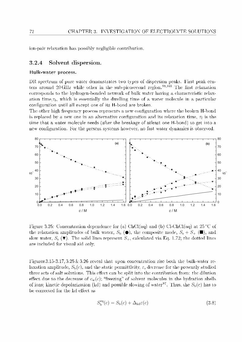
72 CHAPTER 3. INVESTIGATION OF ELECTROLYTE SOLUTIONS
ion-pair relaxation has possibly negligible contribution.
3.2.4 Solvent dispersion.
Bulk-water process.
DR spectrum of pure water demonstrates two types of dispersion peaks. First peak cen-ters around 20GHz while other in the sub-picosecond region.98,163 The rst relaxationcorresponds to the hydrogen-bonded network of bulk water having a characteristic relax-ation time,τb, which is essentially the dwelling time of a water molecule in a particularconguration until all except one of its H-bond are broken.The other high frequency process represents a new conguration where the broken H-bondis replaced by a new one in an alternative conguration and its relaxation time, τf is thetime that a water molecule needs (after the breakage of atleast one H-bond) to get into anew conguration. For the present systems however, no fast water dynamics is observed.
Figure 3.25: Concentration dependence for (a) ChCl(aq) and (b) Cl-ChCl(aq) at 25 C ofthe relaxation amplitudes of bulk water, Sb ( ), the composite mode, Ss + S+ (), andslow water, Ss (H). The solid lines represent S+, calculated via Eq. 1.72; the dotted linesare included for visual aid only.
Figures 3.15-3.17, 3.25&3.26 reveal that upon concentration rise both the bulk-water re-laxation amplitude, Sb(c), and the static permittivity, ε, decrease for the presently studiedthree sets of salt solutions. This eect can be split into the contribution from: the dilutioneect due to the decrease of cw(c); freezing of solvent molecules in the hydration shellsof ions; kinetic depolarization (kd) and possible slowing of water87. Thus, the Sb(c) has tobe corrected for the kd eect as
Seqb (c) = Sb(c) + ∆kdε(c) (3.8)

3.2. DRS OF CHOLINE CHLORIDE, CHLOROCHOLINE CHLORIDE ANDAMMONIUM CHLORIDE 73
0.0 0.5 1.0 1.5 2.0 2.5 3.00
10
20
30
40
50
60
70
80
Si
c / M
Figure 3.26: Concentration dependence of the relaxation amplitudes of bulk water, Sb ( ),and slow water, Ss (), at 25 C for NH4Cl(aq). Dotted lines are included for visual aidonly.
For a solvent with Debye-type relaxation behavior, kd can be expressed as
∆kdε(c) = ξκ(c) (3.9)
and
ξ = p× ε(0)− ε∞(0)
ε(0)× τ(0)
ε0(3.10)
in Eq. 3.10, ε(0) is the static permittivity and τ(0) is the relaxation time of pure wa-ter.170172 The parameter p characterizes the hydrodynamic boundary conditions with p = 1for stick and p = 2/3 for slip type of ionic motion.Here it should be noted that the relaxation time of bulk water mode, τb remains fairlyconstant (Figure 3.27) for ChCl(aq) and decreases (Figures 3.27&3.28) for Cl-ChCl(aq)and NH4Cl(aq) which stems that bulk water dynamics is not aected by the solute in caseof ChCl(aq) while presence of Cl-ChCl and NH4Cl in water do have an eect on the bulkwater dynamics hence Cl-Ch+ and NH+
4 ions aect the water molecules even beyond theirhydration shells, as claimed in literature10,173 for certain electrolytes in water.
Composite process.
As described before in section 3.2.2, the intermediate dispersion mode in case of ChCl(aq)and Cl-ChCl(aq) is assumed to be a composite mode which has contribution from slowwater as well as respective cations in the salt. For NH4Cl(aq), however, this mode isassigned solely to the slow water molecules. Quantitative description of this compositemode has been done with an equation analogous to the Eq. 1.72.

74 CHAPTER 3. INVESTIGATION OF ELECTROLYTE SOLUTIONS
0.0 0.2 0.4 0.6 0.8 1.0 1.2 1.4 1.6
6
8
10
12
14
16
18
i / ps
c / M
Figure 3.27: Concentration dependence of the relaxation time of composite mode, τc, ofChCl(aq) (), bulk-water mode, τb, of ChCl(aq) ( ), and bulk-water mode, τb, of Cl-ChCl(aq)(), at 25 C. Dotted lines are visual aid only.
0.0 0.5 1.0 1.5 2.0 2.5 3.0
5
10
15
20
25
30
i / ps
c / M
Figure 3.28: Concentration dependence of the relaxation time of slow-water mode, τs, (N),and bulk-water mode, τb, (J), of NH4Cl(aq) at 25 C. Dotted lines are visual aid only.
The amplitude of this mode can be split into its constituents as
Sc = S+ + Ss (3.11)
where S+ is the relaxation amplitude due to the rotation of the dipolar Ch+ or Cl− Ch+
ions and Ss is the relaxation amplitude of the slow water molecules hydrating the cation.Similar splitting of the τc is however not permissible as the relaxation rates, τ−1
+ and τ−1s
can not be assumed to be concentration independent, also the τ−1c can not be considered

3.2. DRS OF CHOLINE CHLORIDE, CHLOROCHOLINE CHLORIDE ANDAMMONIUM CHLORIDE 75
as the amplitude-weighted average of the two contributing processes in the compositemode.73 Unfortunately, this hinders the calculation of the activation parameters for slow-water relaxation process, which would be of considerable interest. For Cl-ChCl(aq) system,the τc is xed to a value 15.3 in the tting routine in order to get internally consistentparameters of the ts. This number is the average value of various τc obtained for dierentconcentrations and without xing any parameter. To calculate S+ for both systems Eq. 1.72can be used, hence the Sc can also be evaluated from Eq. 3.11. It is evident from Fig. 3.25that the S+ for Cl− Ch+ is greater than S+ for Ch+ at all the studied concentrations andthis corresponds to the greater dipole moment of Cl− Ch+ ion compared to the Ch+ ion.
3.2.5 Ion hydration.
If the strength of ion-solvent interactions is much greater (strong ion-dipole forces) thanthe solvent-solvent interactions and the kinetics of exchange between the water moleculesin the hydration shell(s) of ion and the bulk water is too slow, then these water molecules(bounded to ions) become eectively immobalized on DRS time scale and are said tobe `frozen' or `irrotationally bound', hence cannot be detected by DRS anymore. Thiseect can be seen for the ions with high surface-charge density in all solvent classes and ismajor cause of decrease in the solvent dispersion amplitude with increasing concentrationof electrolyte.11 In order to calculate the number of frozen water molecules per unit of saltan eective solvation number, Zib, can be dened as
Zib = (cow − capb − caps )/c (3.12)
In a moderate situation, however the water dynamics is not frozen but only slowed downcompared to the bulk-water dynamics. For large hydrophobic solutes such slow-watermolecules in the primary hydration shell are detectable as a separate relaxation processwith τs ≈ 3 τb.12,161,162 The number of water molecules which have been slowed down persalt molecule, Zs, can be evaluated as
Zs = caps /c (3.13)
Two dierent types of hydration numbers obtained in this way are shown in Figures 3.29&3.30.No irrotational bounding of water molecules is observed in aqueous solutions of NH4Cl whilefor both ChCl(aq) and Cl-ChCl(aq) the observed number of frozen-water molecules per re-spective salt molecule at innite dilution is found to be similar i.e., ∼5, this value for eachsystem corresponds to the total salt hence, in order to nd individual ionic contributionsthe value was split by assuming Zib(Cl
−, aq) = 0. This assumption is made due to theobservation that Zib(R4NCl, aq) ≈ 0 when R = methyl (Me) or ethyl (Et) group.12
It is worthwhile here to compare our results with the literature data pertaining to sometetra-n-alkylammonium ions12, where it was observed that Me4NBr, Et4NCl, Et4NBr,Pr4NBr, Bu4NBr and Pe4NBr do not freeze water molecules in their hydration shellswhereas only Pr4NBr, Bu4NBr and Pe4NBr show `hydrophobic hydration' (with Zs ∼ 18.8,36.3 and 44.1, respectivly). MD simmulations of ChCl suggest the formation of weak hy-drogen bonds between cation's OH and the water.164 Based on these observations it would
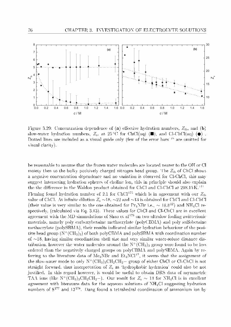
76 CHAPTER 3. INVESTIGATION OF ELECTROLYTE SOLUTIONS
Figure 3.29: Concentration dependence of (a) eective hydration numbers, Zib, and (b)slow-water hydration numbers, Zs, at 25 C for ChCl(aq) (), and Cl-ChCl(aq) ( ) .Dotted lines are included as a visual guide only (few of the error bars174 are omitted forvisual clarity).
be reasonable to assume that the frozen water molecules are located nearer to the OH or Clmoiety then to the bulky positively charged nitrogen head group. The Zib of ChCl showsa negative concentration dependence and no variation is observed for Cl-ChCl, this maysuggest interacting hydration spheres of choline ion, this in principle should also explainthe the dierence in the Waldon product obtained for ChCl and Cl-ChCl at 298.15K.114
Fleming found hydration number of 2.1 for ChCl175 which is in agreement with our Zib
value of ChCl. At innite dilution Zs ∼18, ∼22 and ∼13 is obtained for ChCl and Cl-ChCl(their value is very similar to the one obtained for Pr4NBr i.e., ∼ 18.812) and NH4Cl re-spectively, (calculated via Eq. 3.13). These values for ChCl and Cl-ChCl are in excellentagreement with the MD simmulations of Shao et al176 on two ultralow fouling zwitterionicmaterials, namely poly carboxybetaine methacrylate (polyCBMA) and poly sulfobetainemethacrylate (polySBMA), their results indicated similar hydration behaviour of the posi-tive head group (N+(CH3)3) of both polyCBMA and polySBMA with coordination numberof ∼18, having similar coordination shell size and very similar water-solute distance dis-tribution, however the water molecules around the N+(CH3)3 group were found to be lessordered than the negatively charged groups on polyCBMA and polySBMA. Again by re-ferring to the literature data of Me4NBr and Et4NCl
12, it seems that the assignment ofthe slow-water mode to only N+(CH3)3CH2CH2− group of either ChCl or Cl-ChCl is notstraight forward, thus interpretation of Zs as `hydrophobic hydration' could also be notjustied. In this regard however, it would be useful to obtain DRS data of asymmetricTAA ions (like N+(CH3)3CH2CH2−). Our result for Zs ∼ 13 for NH4Cl is in excellentagreement with literature data for the aqueous solutions of NH4Cl suggesting hydrationnumbers of 8177 and 13178. Dang found a tetrahedral coordination of ammonium ion by

3.2. DRS OF CHOLINE CHLORIDE, CHLOROCHOLINE CHLORIDE ANDAMMONIUM CHLORIDE 77
the water molecules in the rst hydration shell.179
0.0 0.5 1.0 1.5 2.0 2.5 3.00
5
10
15
20
25
30
Z s
c / M
Figure 3.30: Concentration dependence of slow-water hydration number, Zs, for NH4Cl(aq)at 25 C. Dotted lines are included as a visual guide only.
Decrease in the Zs with increasing concentration is observed for all studied electrolytes.It should be noted that the emergence of slow-water dispersion (in the composite mode)is not assumed to be due to the strengthening of H-bonds in the vicinity of solute but tothe increase in number and life time of H-bonds adjacent to the solute.11 NMR studies ofKenneth and his coworkers showed that addition of water to the lowest liquid hydrates (sat-urated solutions) of ChCl resulted in larger and looser hydration shell with the compositionChCl·10H2O (secondary clathrates),180 all these observations point that the hydration shellof ChCl and Cl-ChCl is labile, also the MD simulation of hydrated NH+
4 ion181 suggest arather exible solvation structure around the ion hence a highly labile NH+
4 hydrate.
3.2.6 Temperature dependence of bulk water dynamics.
For the detailed analysis of dynamics of ChCl solutions, spectra of 0.28 molal ChCl weremeasured at at 5, 15, 25, 35, 45, 55, and 65 C. All the spectra tted well in D+D+Dmodel. The rise in temperature is accompanied with the decrease in amplitudes of all DRmodes, where the composite mode can be just detected at 65 C. Vanishing slow watercontribution in the composite mode with temperature rise can be justied as dynamicsget faster, this further implies that the contribution of cation relaxation to the compositemode is very weak and is always dominated by the slow water process. This can be seen inFigure 3.25a (at 25 C) where S+ has weak contribution to Sc. Relevant spectra are shownin Figure 3.18 whereas Figure 3.31 refer to the changes in the various relaxation times withthe changes in the temperature. No signicant changes in the τ1 were observed but theτc and τb decrease signicantly as expected due to faster dynamics of solvent molecules at
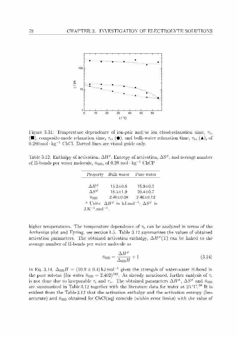
78 CHAPTER 3. INVESTIGATION OF ELECTROLYTE SOLUTIONS
0 10 20 30 40 50 601
10
100
i / ps
t / °C
Figure 3.31: Temperature dependence of ion-pair and/or ion cloud-relaxation time, τ1,(), composite-mode relaxation time, τc, ( ), and bulk-water relaxation time, τb, (N), of0.280mol · kg−1 ChCl. Dotted lines are visual guide only.
Table 3.12: Enthalpy of activation, ∆H=, Entropy of activation, ∆S =, and average numberof H-bonds per water molecule, nHB, of 0.28 mol · kg−1 ChCla
Property Bulk water Pure water
∆H = 15.2±0.6 15.9±0.2∆S = 18.5±1.9 20.4±0.7nHB 2.40±0.08 2.46±0.12
a Units: ∆H = in kJ.mol−1; ∆S = inJ.K−1.mol−1.
higher temperatures. The temperature dependence of τb can be analyzed in terms of theArrhenius plot and Eyring, see section 1.5. Table 3.12 summarizes the values of obtainedactivation parameters. The obtained activation enthalpy, ∆H =(T) can be linked to theaverage number of H-bonds per water molecule as
nHB =∆H =
∆HBH+ 1 (3.14)
In Eq. 3.14, ∆HBH = (10.9 ± 0.4) kJmol−1 gives the strength of water-water H-bond inthe pure solvent (for water nHB = 2.402)182. As already mentioned, further analysis of τcis not done due to inseparable τs and τ+. The obtained parameters ∆H =, ∆S = and nHB
are summarized in Table 3.12 together with the literature data for water at 25 C.98 It isevident from the Table 3.12 that the activation enthalpy and the activation entropy (lessaccurate) and nHB obtained for ChCl(aq) coincide (within error limits) with the value of
3.2. DRS OF CHOLINE CHLORIDE, CHLOROCHOLINE CHLORIDE ANDAMMONIUM CHLORIDE 79
pure water, this is also supported by the constant τb of ChCl(aq) (section 3.2.2), thus, forChCl(aq) ions do not aect the dynamics of bulk-water molecules.


Chapter 4
Investigation of micellar systems
Owing to their amphiphilic nature and special properties like adsorption and self-aggregation,surfactants are widely used in detergents, foaming agents, dispersants, emulsiers, textile,food industry and formulations. Among natural surfactants, the alkali soaps (sodium andpotassium carboxylates) are the oldest and are known since centuries and were preparedfrom tallow and alkali hydroxides.6 Among dierent classes of surfactants, anionics, withcarboxylates, -CO−
2 , sulfates, -OSO−3 , and sulfonates, -SO−
3 , as headgroups are used morefrequently as they are easy to prepare and are more economical, on the other hand cation-ics, with tetramethylammonium ions, -N+(CH3)3, as headgroups are employed as surfacemodiers, anticorrosion agents, otation collectors, bactericides and fabric softeners.183
The solubility of a surfactant is a critical parameter as far as its practical application is con-cerned and generally the clearing temperature of 1wt% surfactant solution, known as Kratpoint,184 is used as a criterion for surfactant's solubility. It is known that Krat pointsof sodium carboxylates are higher, as it ranges from 25 C for sodium laurate, NaC12, to45 C for sodium myristate, NaC14, 60 C for sodium palmitate, NaC16,13,185,186 and 71 Cfor sodium stearate, NaC18.186 Since surfactants with longer alkyl chain have better deter-gency187 and other properties compared to those with short chains, compromising not onthese properties but still attaining lower Krat points was a matter of challenge. At onehand this problem can be solved by modifying the structure of headgroup or alkyl chainbut this generally has negative eects on biodegradability of surfactant.8 It was observedthat the choice of counterion is critical in achieving this goal188 and tetraalkylammoniumions, TAA, were found to be a better choice than sodium with carboxylates.189,190 It isclaimed that surfactants having choline as counter-ions are able to substitute those withtetraalkylammonium counter-ions as TAA ions are toxic, whereas choline is non-toxic andbiologically degradable.14 It should be noted that choline is also part of a natural surfac-tant, dipalmitoylphosphatidylcholine which is crucial for the normal lung functioning. Inaddition to choline carboxylates, another biocompatible surfactant, choline dodecylsulfate,was prepared and patented by the University of Regensburg.7
Figure 4.1 taken from the literature data of Vlachy et al.191 represents the suitability ofcoupling among various types of headgroups and cations. In principle, choline ion (Ch+)could be the next member of this cationic series, i.e. Li+..→..NH+
4 → Ch+, hence softestamong the displayed cations. As expected the binding between carboxylate headgroup
81
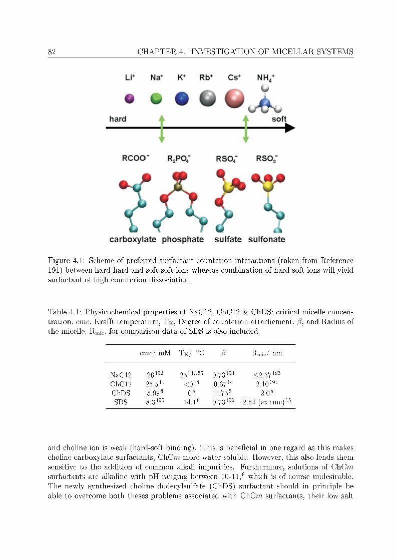
82 CHAPTER 4. INVESTIGATION OF MICELLAR SYSTEMS
Figure 4.1: Scheme of preferred surfactant-counterion interactions (taken from Reference191) between hard-hard and soft-soft ions whereas combination of hard-soft ions will yieldsurfactant of high counterion dissociation.
Table 4.1: Physicochemical properties of NaC12, ChC12 & ChDS: critical micelle concen-tration, cmc; Krat temperature, TK; Degree of counterion attachement, β; and Radius ofthe micelle, Rmic, for comparison data of SDS is also included.
cmc/ mM TK/C β Rmic/ nm
NaC12 26192 2513,185 0.73193 ≤2.37193ChC12 25.514 <014 0.6714 2.10194
ChDS 5.998 08 0.758 2.08
SDS 8.3195 14.18 0.73196 2.64 (at cmc)15
and choline ion is weak (hard-soft binding). This is benecial in one regard as this makescholine carboxylate surfactants, ChCm more water soluble. However, this also lends themsensitive to the addition of common alkali impurities. Furthermore, solutions of ChCmsurfactants are alkaline with pH ranging between 10-11,8 which is of course undesirable.The newly synthesized choline dodecylsulfate (ChDS) surfactant should in principle beable to overcome both theses problems associated with ChCm surfactants, their low salt
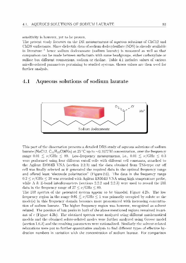
4.1. AQUEOUS SOLUTIONS OF SODIUM LAURATE 83
sensitivity is however, yet to be proven.The present study focusses on the DR measurements of aqueous solutions of ChC12 andChDS surfactants. Since dielectric data of sodium dodecylsulfate (SDS) is already availablein literature15 hence sodium dodecanoate (sodium laurate) is measured as well so thatcomparison can be made between surfactants with same headgroups, either carboxylate orsulfate but dierent counterions, sodium or choline. Table 4.1 includes values of variousmicelle-related parameters pertaining to studied systems, theses values are then used forfurther analysis.
4.1 Aqueous solutions of sodium laurate
This part of the dissertation presents a detailed DRS study of aqueous solutions of sodiumlaurate (NaC12, C11H23C00Na) at 25 C up to ∼0.1077M concentration, over the frequencyrange 0.01 . ν/GHz ≤ 89. Low-frequency measurements, i.e., 0.01 . ν/GHz ≤ 0.3were performed using four dierent cuto cells with dierent cell constants, attached tothe Agilent E8364B VNA (section 2.2.3) and the data obtained from TS3-type cut ocell was nally selected as it generated the required data in the optimal frequency rangeand oered least electrode polarization (Figure 2.6). The data in the frequency range0.2 ≤ ν/GHz ≤ 20 was recorded with Agilent E8364B VNA using high temperature probe,while A & E-band interferometers (sections 2.2.2 and 2.2.3) were used to record the DRdata in the frequency range of 27 ≤ ν/GHz ≤ 89.The DR spectra of the presented system appear to be bimodal, Figure 4.2b. The lowfrequency region in the range 0.01 . ν/GHz ≤ 1 was primarily occupied by solute as themode(s) in this frequency domain becomes more pronounced with increasing concentra-tion of sodium laurate. The higher frequency region was however, recognized as solventrelated. The position of loss peaks in both of the above mentioned regions remained invari-ant of c (Figure 4.2b). The obtained spectra were analyzed using dierent mathematicalmodels and the obtained solute-related modes were further analyzed using Grosse model(section 1.6.3) and the resulting parameters were rationalized. Similarly the solvent-relatedrelaxations were put to further quantitative analysis to nd dierent types of eective hy-dration numbers in variation with the concentration of sodium laurate. For comparison
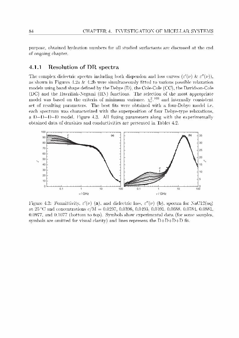
84 CHAPTER 4. INVESTIGATION OF MICELLAR SYSTEMS
purpose, obtained hydration numbers for all studied surfactants are discussed at the endof ongoing chapter.
4.1.1 Resolution of DR spectra
The complex dielectric spectra including both dispersion and loss curves (ε′(ν) & ε′′(ν)),as shown in Figures 4.2a & 4.2b were simultaneously tted to various possible relaxationmodels using band shape dened by the Debye (D), the Cole-Cole (CC), the Davidson-Cole(DC) and the Havriliak-Negami (HN) functions. The selection of the most appropriatemodel was based on the criteria of minimum variance, χ2
r ,103 and internally consistent
set of resulting parameters. The best ts were obtained with a four-Debye model i.e.each spectrum was characterized with the superposition of four Debye-type relaxations,a D+D+D+D model, Figure 4.3. All tting parameters along with the experimentallyobtained data of densities and conductivities are presented in Tables 4.2.
Figure 4.2: Permittivity, ε′(ν) (a), and dielectric loss, ε′′(ν) (b), spectra for NaC12(aq)at 25 C and concentrations c/M = 0.0297, 0.0396, 0.0493, 0.0591, 0.0688, 0.0784, 0.0881,0.0977, and 0.1077 (bottom to top). Symbols show experimental data (for some samples,symbols are omitted for visual clarity) and lines represent the D+D+D+D t.
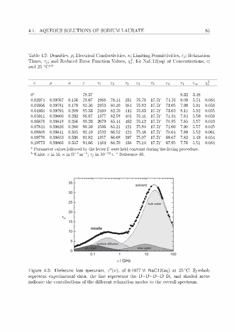
4.1. AQUEOUS SOLUTIONS OF SODIUM LAURATE 85
Table 4.2: Densities, ρ; Electrical Conductivities, κ; Limiting Permittivities, εj; RelaxationTimes, τj; and Reduced Error Function Values, χ2
r , for NaC12(aq) at Concentrations, c;and 25 Ca,b
c ρ κ ε τ1 ε2 τ2 ε3 τ3 ε4 τ4 ε∞ χ2r
0c 78.37 8.32 3.480.02974 0.99767 0.156 79.67 1968 78.14 231 76.78 17.7F 74.76 8.09 5.74 0.0840.03956 0.99781 0.179 82.56 2353 80.20 384 76.82 17.7F 73.05 7.99 5.91 0.0500.04934 0.99794 0.209 85.33 2460 82.70 444 76.63 17.7F 73.63 8.11 5.92 0.0550.05911 0.99806 0.232 86.87 1377 82.58 404 76.41 17.7F 71.34 7.84 5.50 0.0500.06878 0.99818 0.256 89.23 2079 85.44 462 76.12 17.7F 70.85 7.85 5.57 0.0430.07844 0.99826 0.280 90.59 1506 85.21 421 75.80 17.7F 71.00 7.90 5.57 0.0450.08808 0.99841 0.305 92.19 1532 86.52 424 75.48 17.7F 70.64 7.89 5.52 0.0610.09770 0.99853 0.330 92.82 1357 86.08 397 75.07 17.7F 69.67 7.82 5.49 0.0540.10773 0.99866 0.357 94.66 1464 88.70 438 75.10 17.7F 67.95 7.76 5.51 0.084a Parameter values followed by the letter F were held constant during the tting procedure.b Units: c in M, κ in Ω−1m−1; τj in 10−12 s. c Reference 86.
Figure 4.3: Dielectric loss spectrum, ε′′(ν), of 0.1077M NaC12(aq) at 25 C. Symbolsrepresent experimental data, the line represents the D+D+D+D t, and shaded areasindicate the contributions of the dierent relaxation modes to the overall spectrum.
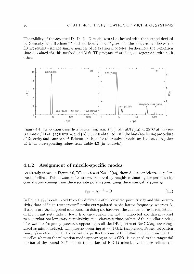
86 CHAPTER 4. INVESTIGATION OF MICELLAR SYSTEMS
The validity of the accepted D+D+D+D model was also checked with the method devisedby Zasetzky and Buchner105 and as depicted by Figure 4.4, the analysis reinforces thetting results with the similar number of relaxation processes, furthermore the relaxationtimes obtained via this method and MWFIT program103 are in good agreement with eachother.
Figure 4.4: Relaxation time distribution function, P (τ), of NaC12(aq) at 25 C at concen-trations c / M of: (a) 0.02974, and (b) 0.09770 obtained with the bias-free tting procedureof Zasetzky and Buchner.105 Relaxation times for the resolved modes are indicated togetherwith the corresponding values from Table 4.2 (in brackets).
4.1.2 Assignment of micelle-specic modes
As already shown in Figure 2.6, DR spectra of NaC12(aq) showed distinct electrode polar-ization eect. This unwanted feature was removed by roughly estimating the permittivitycontribution coming from the electrode polarization, using the empirical relation as
ε′EP = Aν−α + B (4.1)
In Eq. 4.1 ε′EP is calculated from the dierence of uncorrected permittivity and the permit-tivity data of high temperature probe extrapolated to the lowest frequency, whereas A,B and α are the empirical constants. In doing so, however, the chances of over correctionof the permittivity data at lower frequency region can not be neglected and this may leadto somewhat too low static permittivity and relaxation times values of the micellar modes.The two low-frequency processes appearing in all the DR spectra of NaC12(aq) are recog-nized as micelle-related. The process occurring at ∼0.1GHz (amplitude, S1 and relaxationtime, τ1) is attributed to the radial charge uctuations of the diuse ion cloud around themicelles whereas the relaxation mode appearing at ∼0.4GHz, is assigned to the tangentialmotion of the bound Na+ ions at the surface of NaC12 micelles and hence reects the
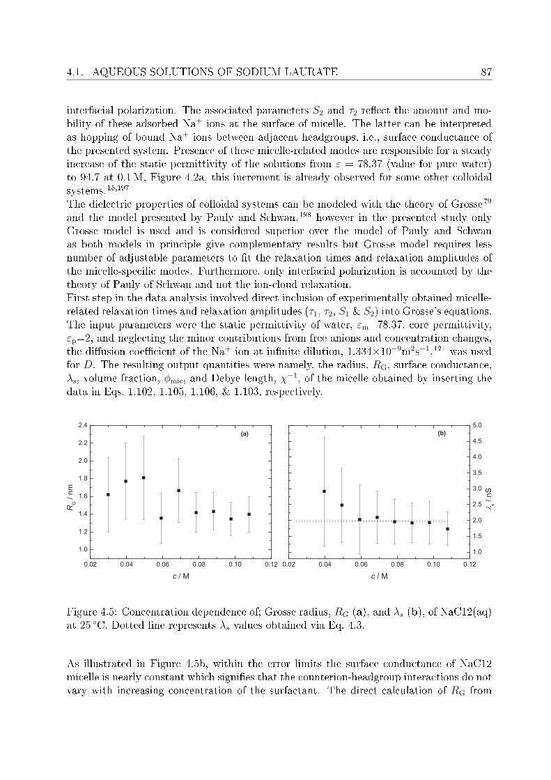
4.1. AQUEOUS SOLUTIONS OF SODIUM LAURATE 87
interfacial polarization. The associated parameters S2 and τ2 reect the amount and mo-bility of these adsorbed Na+ ions at the surface of micelle. The latter can be interpretedas hopping of bound Na+ ions between adjacent headgroups, i.e., surface conductance ofthe presented system. Presence of these micelle-related modes are responsible for a steadyincrease of the static permittivity of the solutions from ε = 78.37 (value for pure water)to 94.7 at 0.1M, Figure 4.2a, this increment is already observed for some other colloidalsystems.15,197
The dielectric properties of colloidal systems can be modeled with the theory of Grosse79
and the model presented by Pauly and Schwan,198 however in the presented study onlyGrosse model is used and is considered superior over the model of Pauly and Schwanas both models in principle give complementary results but Grosse model requires lessnumber of adjustable parameters to t the relaxation times and relaxation amplitudes ofthe micelle-specic modes. Furthermore, only interfacial polarization is accounted by thetheory of Pauly of Schwan and not the ion-cloud relaxation.First step in the data analysis involved direct inclusion of experimentally obtained micelle-related relaxation times and relaxation amplitudes (τ1, τ2, S1 & S2) into Grosse's equations.The input parameters were the static permittivity of water, εm=78.37, core permittivity,εp=2, and neglecting the minor contributions from free anions and concentration changes,the diusion coecient of the Na+ ion at innite dilution, 1.334×10⁻⁹m2s−1,121 was usedfor D. The resulting output quantities were namely, the radius, RG, surface conductance,λs, volume fraction, ϕmic, and Debye length, χ−1, of the micelle obtained by inserting thedata in Eqs. 1.102, 1.105, 1.106, & 1.103, respectively.
Figure 4.5: Concentration dependence of; Grosse radius, RG (a), and λs (b), of NaC12(aq)at 25 C. Dotted line represents λs values obtained via Eq. 4.3.
As illustrated in Figure 4.5b, within the error limits the surface conductance of NaC12micelle is nearly constant which signies that the counterion-headgroup interactions do notvary with increasing concentration of the surfactant. The direct calculation of RG from

88 CHAPTER 4. INVESTIGATION OF MICELLAR SYSTEMS
the experimental τ1 values results in values ranging between 1.2 and 1.8 nm (Figure 4.5a),which is considerably smaller than experimental data from small-angle neutron scattering(SANS) method ranging from 2.37 nm at 0.16M to 2.58 nm at 0.53M.193 Due to this reasonthe obtained values of RG (Figure 4.5a) were not used for further calculations, rather RG
was used as an adjustable parameter for further calculations. Furthermore, it was observedthat the χ−1 values, obtained from the tting of experimental data into Eq. 1.103, in thestudied concentration range could be presented as
χ−1 = [0.57 + 2.20× c] nm (4.2)
The obtained ϕmic values are shown in Figure 4.8. In the next step of analysis the simulta-neous tting of micelle-related relaxation times and relaxation amplitudes was performedby using two adjustable parameters namely the micellar radius, RG and tangential diu-sion coecient of the sodium ions condensed on the micellar surface, Ds
+, and from theequations of reference 79, following relation was employed to evaluate λs.
Ds+ =
4πkBTλsR2G
e2βNag
(4.3)
Where β denotes the degree of counterion attachment and e is the elementary charge.Eq. 4.3 & Eq. 1.101 alone were employed to obtain another set of values for λs and ϕmic,hence do not involve the use of experimental amplitudes or relaxation times. The corre-sponding results are displayed in the form of dotted lines in Figures 4.5b & 4.8.A constant value of micellar aggregation number, Nag of 89 was taken from literature.199
It should be noted that the molecular dynamics study of the sodium laurate plus watersystem does show the progression from spherical through elongated and worm micellesto lamellar phases.200 However, upto 10% (weight percent) only spherical micelles prevailand for the presented work, where the concentration was not more than 2.4%, Nag can beused as a constant, hence similar argument can be used for the constant RG. Also, it wasassumed that above critical micelle concentration, cmc the concentration of free monomers,cf is equal to the cmc. In addition to the use of RG and Ds
+ as adjustable parameters,experimental conductivities were used as κm, while a core conductivity of κc=0 was usedas the inner core of the micelle is considered as pure hydrocarbon. Moreover, χ−1 valuesrepresented by Eq. 4.2 and Eq. 1.104 were also used in the data analysis and the resultsobtained from both equations were then compared. The rest of input parameters weresame as already mentioned in preceding paragraph, i.e., standard values of εm, εp and D,together with the degree of counterion attachment, β=0.73, estimated from the literaturedata of Caponetti et al.193 The micellar radius was adjusted to the value of 2.50 nm as thisvalue yielded excellent description of S1 & S2 and τ2 over the entire concentration range(Figures 4.6 & 4.7).The experimental values of τ1 always lie below the Grosse's predicted values which mightbe due to under estimation of ion-cloud relaxation times resulting from the correction forelectrode polarization. After correcting the adjusted value of RG for the radius of Na+
ion (0.12 nm18) as RG = Rmic + RNa+ , the micellar radius agrees well with the literaturedata,193 hence, it can be reasonably inferred that the counter sodium ions are in directcontact with the carboxylate headgroup of the NaC12 micelle (Figures 4.26). this
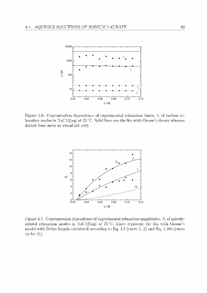
4.1. AQUEOUS SOLUTIONS OF SODIUM LAURATE 89
0.02 0.04 0.06 0.08 0.10 0.12
10
100
1000
10000
4
3
2
i / ps
c / M
1
Figure 4.6: Concentration dependence of experimental relaxation times, τi of various re-laxation modes in NaC12(aq) at 25 C. Solid lines are the ts with Grosse's theory whereasdotted lines serve as visual aid only.
0.02 0.04 0.06 0.08 0.10 0.120
2
4
6
8
10
12
14
2
1a
S2
Si
c / M
S1
1
Figure 4.7: Concentration dependence of experimental relaxation amplitudes, Si of micelle-related relaxation modes in NaC12(aq) at 25 C. Lines represent the ts with Grosse'smodel with Debye length calculated according to Eq. 4.2 (curve 1, 2) and Eq. 1.104 (curve1a for S1).
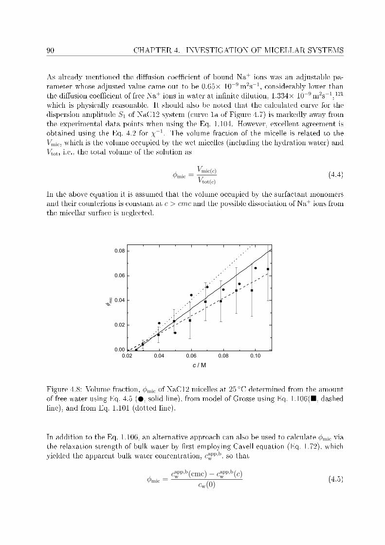
90 CHAPTER 4. INVESTIGATION OF MICELLAR SYSTEMS
As already mentioned the diusion coecient of bound Na+ ions was an adjustable pa-rameter whose adjusted value came out to be 0.65× 10⁻⁹m2s−1, considerably lower thanthe diusion coecient of free Na+ ions in water at innite dilution, 1.334× 10⁻⁹m2s−1,121
which is physically reasonable. It should also be noted that the calculated curve for thedispersion amplitude S1 of NaC12 system (curve 1a of Figure 4.7) is markedly away fromthe experimental data points when using the Eq. 1.104. However, excellent agreement isobtained using the Eq. 4.2 for χ−1. The volume fraction of the micelle is related to theVmic, which is the volume occupied by the wet micelles (including the hydration water) andVtot, i.e., the total volume of the solution as
ϕmic =Vmic(c)
Vtot(c)
(4.4)
In the above equation it is assumed that the volume occupied by the surfactant monomersand their counterions is constant at c > cmc and the possible dissociation of Na+ ions fromthe micellar surface is neglected.
0.02 0.04 0.06 0.08 0.100.00
0.02
0.04
0.06
0.08
m
ic
c / M
Figure 4.8: Volume fraction, ϕmic of NaC12 micelles at 25 C determined from the amountof free water using Eq. 4.5 ( , solid line), from model of Grosse using Eq. 1.106(, dashedline), and from Eq. 1.101 (dotted line).
In addition to the Eq. 1.106, an alternative approach can also be used to calculate ϕmic viathe relaxation strength of bulk water by rst employing Cavell equation (Eq. 1.72), whichyielded the apparent bulk water concentration, capp,bw , so that
ϕmic =capp,bw (cmc)− capp,bw (c)
cw(0)(4.5)
4.1. AQUEOUS SOLUTIONS OF SODIUM LAURATE 91
Eq. 4.5 yields the volume fraction of the micelles in the solution including all types ofhydration water, namely slow and frozen water, which is not easily accessible fromthe other experimental methods.197 As depicted in Figure 4.8, ϕmic values calculated fromEq. 1.106 are slightly lower than the one obtained from the analysis of solvent relaxationprocesses via Eq. 4.5. However, the agreement is good between the values obtained viaEq. 4.5 and Eq. 1.101, this supports the acceptance of superposition of four Debye equations(4D) for the presented system.
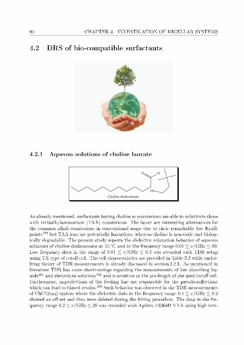
92 CHAPTER 4. INVESTIGATION OF MICELLAR SYSTEMS
4.2 DRS of bio-compatible surfactants
4.2.1 Aqueous solutions of choline laurate
HO
N+
O O-
Choline dodecanoate
As already mentioned, surfactants having choline as counterions are able to substitute thosewith tetraalkylammonium (TAA) counterions. The latter are interesting alternatives forthe common alkali counterions in conventional soaps due to their remarkably low Kratpoints189 but TAA ions are potentially hazardous, whereas choline is non-toxic and biolog-ically degradable. The present study reports the dielectric relaxation behavior of aqueoussolutions of choline dodecanoate at 25 C and in the frequency range 0.01 . ν/GHz ≤ 89.Low frequency data in the range of 0.01 . ν/GHz ≤ 0.2 was recorded with TDR setupusing TX type of cuto cell. The cell characteristics are provided in Table 2.2 while under-lying theory of TDR measurements is already discussed in section 2.2.1. As mentioned inliterature TDR has some shortcomings regarding the measurements of low absorbing liq-uids201 and electrolyte solutions202 and is sensitive to the pin-length of the used cuto cell.Furthermore, imperfections of the feeding line are responsible for the pseudo-reectionswhich can lead to biased results.202 Such behavior was observed in the TDR measurementsof ChC12(aq) system where the dielectric data in the frequency range 0.1 . ν/GHz . 0.2showed an o set and thus were deleted during the tting procedure. The data in the fre-quency range 0.2 ≤ ν/GHz ≤ 20 was recorded with Agilent E8364B VNA using high tem-
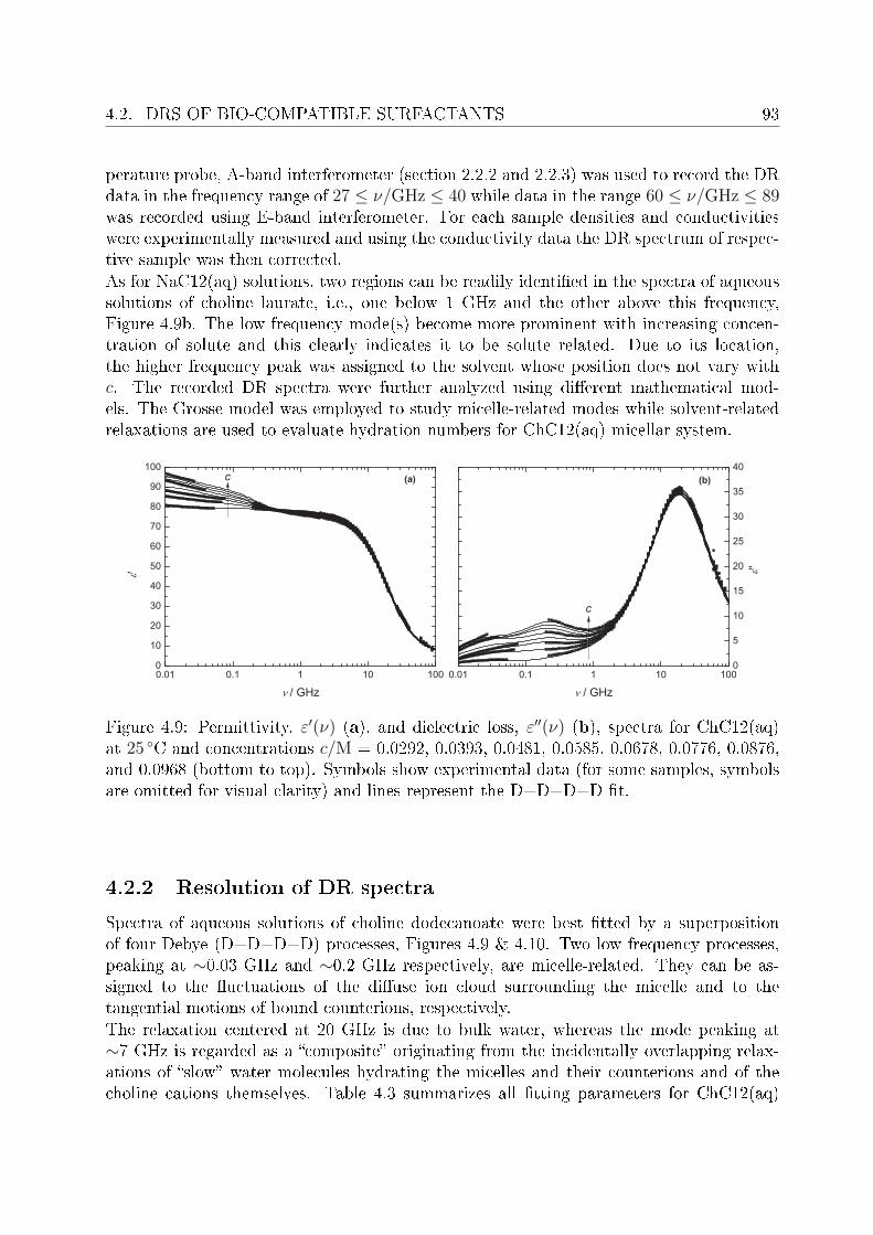
4.2. DRS OF BIO-COMPATIBLE SURFACTANTS 93
perature probe, A-band interferometer (section 2.2.2 and 2.2.3) was used to record the DRdata in the frequency range of 27 ≤ ν/GHz ≤ 40 while data in the range 60 ≤ ν/GHz ≤ 89was recorded using E-band interferometer. For each sample densities and conductivitieswere experimentally measured and using the conductivity data the DR spectrum of respec-tive sample was then corrected.As for NaC12(aq) solutions, two regions can be readily identied in the spectra of aqueoussolutions of choline laurate, i.e., one below 1 GHz and the other above this frequency,Figure 4.9b. The low frequency mode(s) become more prominent with increasing concen-tration of solute and this clearly indicates it to be solute related. Due to its location,the higher frequency peak was assigned to the solvent whose position does not vary withc. The recorded DR spectra were further analyzed using dierent mathematical mod-els. The Grosse model was employed to study micelle-related modes while solvent-relatedrelaxations are used to evaluate hydration numbers for ChC12(aq) micellar system.
Figure 4.9: Permittivity, ε′(ν) (a), and dielectric loss, ε′′(ν) (b), spectra for ChC12(aq)at 25 C and concentrations c/M = 0.0292, 0.0393, 0.0481, 0.0585, 0.0678, 0.0776, 0.0876,and 0.0968 (bottom to top). Symbols show experimental data (for some samples, symbolsare omitted for visual clarity) and lines represent the D+D+D+D t.
4.2.2 Resolution of DR spectra
Spectra of aqueous solutions of choline dodecanoate were best tted by a superpositionof four Debye (D+D+D+D) processes, Figures 4.9 & 4.10. Two low frequency processes,peaking at ∼0.03 GHz and ∼0.2 GHz respectively, are micelle-related. They can be as-signed to the uctuations of the diuse ion cloud surrounding the micelle and to thetangential motions of bound counterions, respectively.The relaxation centered at 20 GHz is due to bulk water, whereas the mode peaking at∼7 GHz is regarded as a composite originating from the incidentally overlapping relax-ations of slow water molecules hydrating the micelles and their counterions and of thecholine cations themselves. Table 4.3 summarizes all tting parameters for ChC12(aq)
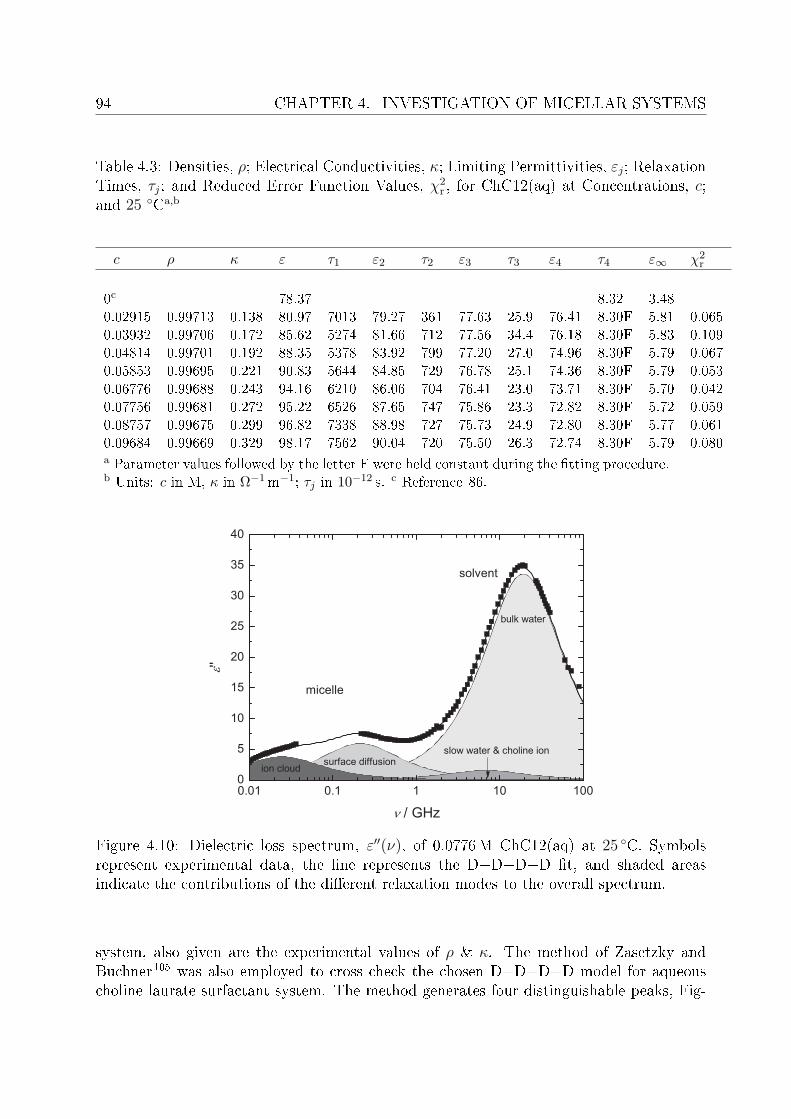
94 CHAPTER 4. INVESTIGATION OF MICELLAR SYSTEMS
Table 4.3: Densities, ρ; Electrical Conductivities, κ; Limiting Permittivities, εj; RelaxationTimes, τj; and Reduced Error Function Values, χ2
r , for ChC12(aq) at Concentrations, c;and 25 Ca,b
c ρ κ ε τ1 ε2 τ2 ε3 τ3 ε4 τ4 ε∞ χ2r
0c 78.37 8.32 3.480.02915 0.99713 0.138 80.97 7013 79.27 361 77.63 25.9 76.41 8.30F 5.81 0.0650.03932 0.99706 0.172 85.62 5274 81.66 712 77.56 34.4 76.18 8.30F 5.83 0.1090.04814 0.99701 0.192 88.35 5378 83.92 799 77.20 27.0 74.96 8.30F 5.79 0.0670.05853 0.99695 0.221 90.83 5644 84.85 729 76.78 25.1 74.36 8.30F 5.79 0.0530.06776 0.99688 0.243 94.16 6210 86.06 704 76.41 23.0 73.71 8.30F 5.70 0.0420.07756 0.99681 0.272 95.22 6526 87.65 747 75.86 23.3 72.82 8.30F 5.72 0.0590.08757 0.99675 0.299 96.82 7338 88.98 727 75.73 24.9 72.80 8.30F 5.77 0.0610.09684 0.99669 0.329 98.17 7562 90.04 720 75.50 26.3 72.74 8.30F 5.79 0.080a Parameter values followed by the letter F were held constant during the tting procedure.b Units: c in M, κ in Ω−1m−1; τj in 10−12 s. c Reference 86.
Figure 4.10: Dielectric loss spectrum, ε′′(ν), of 0.0776M ChC12(aq) at 25 C. Symbolsrepresent experimental data, the line represents the D+D+D+D t, and shaded areasindicate the contributions of the dierent relaxation modes to the overall spectrum.
system, also given are the experimental values of ρ & κ. The method of Zasetzky andBuchner105 was also employed to cross check the chosen D+D+D+D model for aqueouscholine laurate surfactant system. The method generates four distinguishable peaks, Fig-
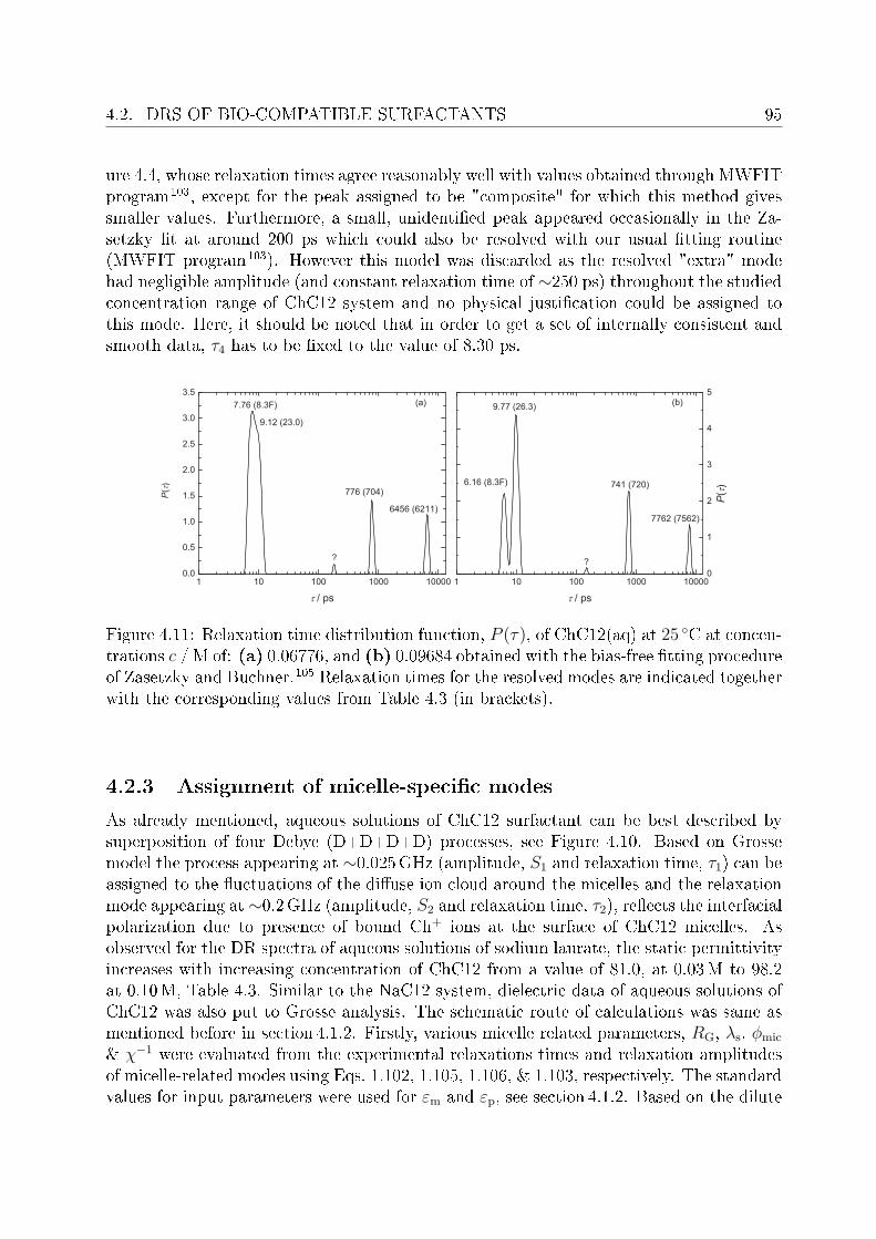
4.2. DRS OF BIO-COMPATIBLE SURFACTANTS 95
ure 4.4, whose relaxation times agree reasonably well with values obtained through MWFITprogram103, except for the peak assigned to be "composite" for which this method givessmaller values. Furthermore, a small, unidentied peak appeared occasionally in the Za-setzky t at around 200 ps which could also be resolved with our usual tting routine(MWFIT program103). However this model was discarded as the resolved "extra" modehad negligible amplitude (and constant relaxation time of ∼250 ps) throughout the studiedconcentration range of ChC12 system and no physical justication could be assigned tothis mode. Here, it should be noted that in order to get a set of internally consistent andsmooth data, τ4 has to be xed to the value of 8.30 ps.
Figure 4.11: Relaxation time distribution function, P (τ), of ChC12(aq) at 25 C at concen-trations c / M of: (a) 0.06776, and (b) 0.09684 obtained with the bias-free tting procedureof Zasetzky and Buchner.105 Relaxation times for the resolved modes are indicated togetherwith the corresponding values from Table 4.3 (in brackets).
4.2.3 Assignment of micelle-specic modes
As already mentioned, aqueous solutions of ChC12 surfactant can be best described bysuperposition of four Debye (D+D+D+D) processes, see Figure 4.10. Based on Grossemodel the process appearing at ∼0.025GHz (amplitude, S1 and relaxation time, τ1) can beassigned to the uctuations of the diuse ion cloud around the micelles and the relaxationmode appearing at∼0.2GHz (amplitude, S2 and relaxation time, τ2), reects the interfacialpolarization due to presence of bound Ch+ ions at the surface of ChC12 micelles. Asobserved for the DR spectra of aqueous solutions of sodium laurate, the static permittivityincreases with increasing concentration of ChC12 from a value of 81.0, at 0.03M to 98.2at 0.10M, Table 4.3. Similar to the NaC12 system, dielectric data of aqueous solutions ofChC12 was also put to Grosse analysis. The schematic route of calculations was same asmentioned before in section 4.1.2. Firstly, various micelle related parameters, RG, λs, ϕmic
& χ−1 were evaluated from the experimental relaxations times and relaxation amplitudesof micelle-related modes using Eqs. 1.102, 1.105, 1.106, & 1.103, respectively. The standardvalues for input parameters were used for εm and εp, see section 4.1.2. Based on the dilute
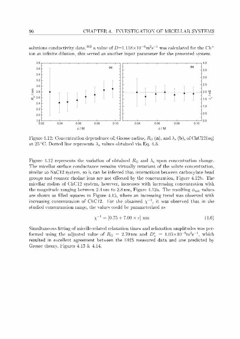
96 CHAPTER 4. INVESTIGATION OF MICELLAR SYSTEMS
solutions conductivity data,203 a value of D=1.118×10⁻⁹m2s−1 was calculated for the Ch+
ion at innite dilution, this served as another input parameter for the presented system.
Figure 4.12: Concentration dependence of; Grosse radius, RG (a), and λs (b), of ChC12(aq)at 25 C. Dotted line represents λs values obtained via Eq. 4.3.
Figure 4.12 represents the variation of obtained RG and λs upon concentration change.The micellar surface conductance remains virtually invariant of the solute concentration,similar to NaC12 system, so it can be inferred that interactions between carboxylate headgroups and counter choline ions are not eected by the concentration, Figure 4.12b. Themicellar radius of ChC12 system, however, increases with increasing concentration withthe magnitude ranging between 2.4 nm to 2.8 nm, Figure 4.12a. The resulting ϕmic valuesare shown as lled squares in Figure 4.15, where an increasing trend was observed withincreasing concentration of ChC12. For the obtained χ−1, it was observed that in thestudied concentration range, the values could be parameterized as
χ−1 = [0.75 + 7.00× c] nm (4.6)
Simultaneous tting of micelle-related relaxation times and relaxation amplitudes was per-formed using the adjusted value of RG = 2.70 nm and Ds
+ = 1.05×10⁻⁹m2s−1, whichresulted in excellent agreement between the DRS measured data and one predicted byGrosse theory, Figures 4.13 & 4.14.
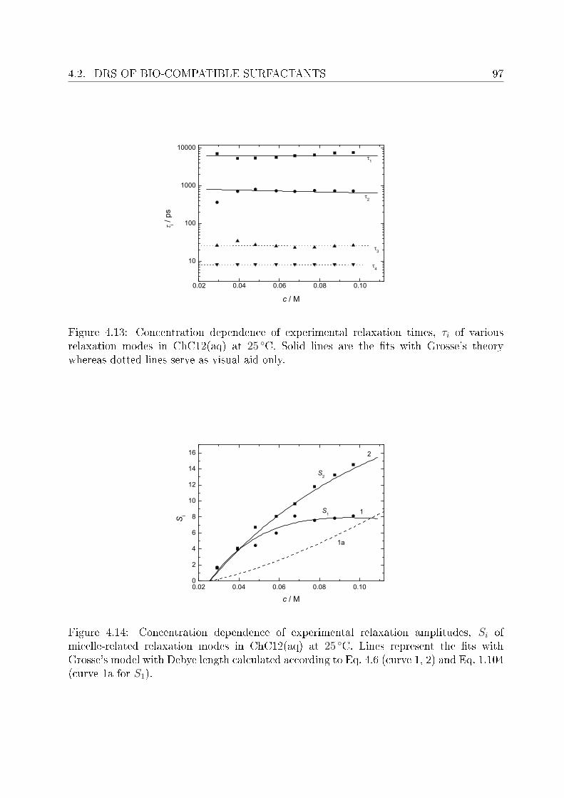
4.2. DRS OF BIO-COMPATIBLE SURFACTANTS 97
0.02 0.04 0.06 0.08 0.10
10
100
1000
10000
4
3
2
1
i / ps
c / M
Figure 4.13: Concentration dependence of experimental relaxation times, τi of variousrelaxation modes in ChC12(aq) at 25 C. Solid lines are the ts with Grosse's theorywhereas dotted lines serve as visual aid only.
0.02 0.04 0.06 0.08 0.100
2
4
6
8
10
12
14
16
1a
1
2
S1
S2
Si
c / M
Figure 4.14: Concentration dependence of experimental relaxation amplitudes, Si ofmicelle-related relaxation modes in ChC12(aq) at 25 C. Lines represent the ts withGrosse's model with Debye length calculated according to Eq. 4.6 (curve 1, 2) and Eq. 1.104(curve 1a for S1).
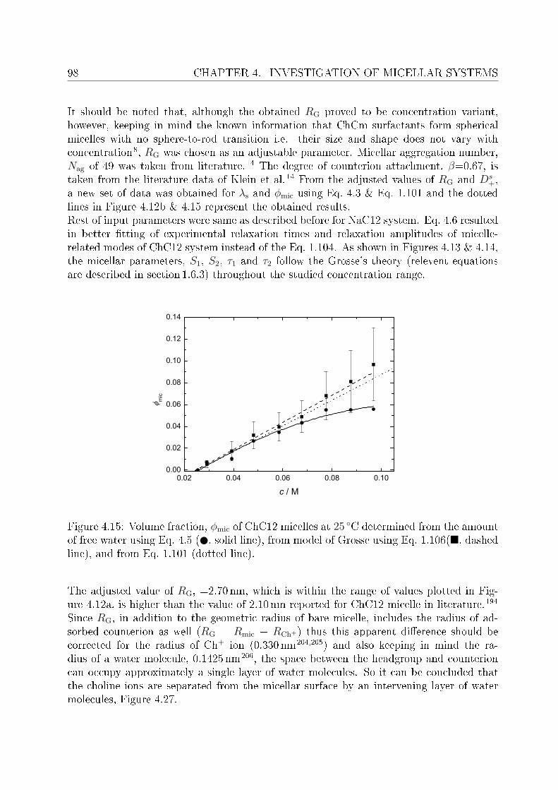
98 CHAPTER 4. INVESTIGATION OF MICELLAR SYSTEMS
It should be noted that, although the obtained RG proved to be concentration variant,however, keeping in mind the known information that ChCm surfactants form sphericalmicelles with no sphere-to-rod transition i.e. their size and shape does not vary withconcentration8, RG was chosen as an adjustable parameter. Micellar aggregation number,Nag of 49 was taken from literature.14 The degree of counterion attachment, β=0.67, istaken from the literature data of Klein et al.14 From the adjusted values of RG and Ds
+,a new set of data was obtained for λs and ϕmic using Eq. 4.3 & Eq. 1.101 and the dottedlines in Figure 4.12b & 4.15 represent the obtained results.Rest of input parameters were same as described before for NaC12 system. Eq. 4.6 resultedin better tting of experimental relaxation times and relaxation amplitudes of micelle-related modes of ChC12 system instead of the Eq. 1.104. As shown in Figures 4.13 & 4.14,the micellar parameters, S1, S2, τ1 and τ2 follow the Grosse's theory (relevent equationsare described in section 1.6.3) throughout the studied concentration range.
0.02 0.04 0.06 0.08 0.100.00
0.02
0.04
0.06
0.08
0.10
0.12
0.14
m
ic
c / M
Figure 4.15: Volume fraction, ϕmic of ChC12 micelles at 25 C determined from the amountof free water using Eq. 4.5 ( , solid line), from model of Grosse using Eq. 1.106(, dashedline), and from Eq. 1.101 (dotted line).
The adjusted value of RG, =2.70 nm, which is within the range of values plotted in Fig-ure 4.12a, is higher than the value of 2.10 nm reported for ChC12 micelle in literature.194
Since RG, in addition to the geometric radius of bare micelle, includes the radius of ad-sorbed counterion as well (RG = Rmic + RCh+) thus this apparent dierence should becorrected for the radius of Ch+ ion (0.330 nm204,205) and also keeping in mind the ra-dius of a water molecule, 0.1425 nm206, the space between the headgroup and counterioncan occupy approximately a single layer of water molecules. So it can be concluded thatthe choline ions are separated from the micellar surface by an intervening layer of watermolecules, Figure 4.27.

4.2. DRS OF BIO-COMPATIBLE SURFACTANTS 99
Volume fraction of ChC12 was calculated with the help of Eq. 1.106, 1.101 and 4.5,Figure 4.15. Upto 0.05M concentration ϕmic obtained from dierent equations agree wellbut after this concentration the curves deviate with slightly higher values coming from theGrosse model, Eq. 1.101 & 1.106.
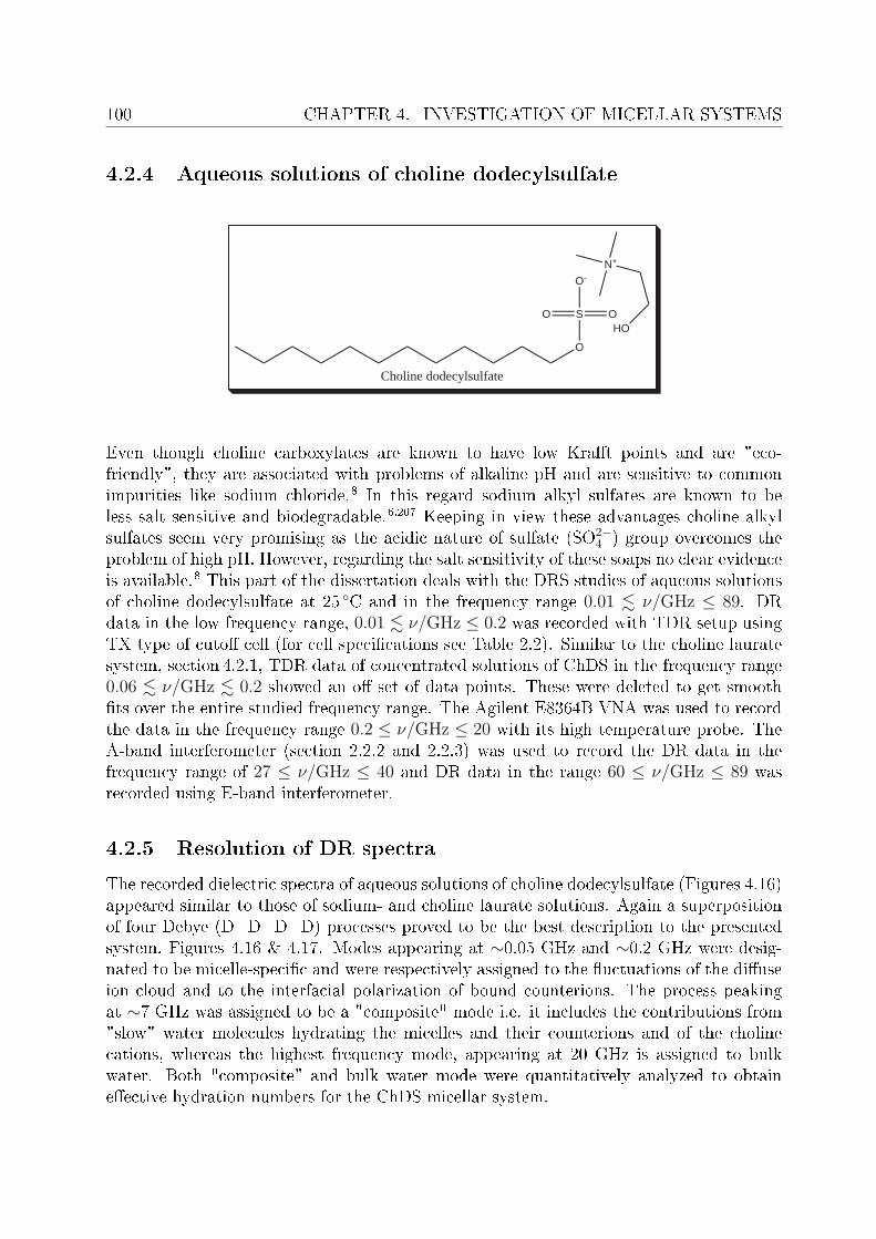
100 CHAPTER 4. INVESTIGATION OF MICELLAR SYSTEMS
4.2.4 Aqueous solutions of choline dodecylsulfate
HO
N+
SO O
O
O-
Choline dodecylsulfate
Even though choline carboxylates are known to have low Krat points and are "eco-friendly", they are associated with problems of alkaline pH and are sensitive to commonimpurities like sodium chloride.8 In this regard sodium alkyl sulfates are known to beless salt sensitive and biodegradable.6,207 Keeping in view these advantages choline alkylsulfates seem very promising as the acidic nature of sulfate (SO2−
4 ) group overcomes theproblem of high pH. However, regarding the salt sensitivity of these soaps no clear evidenceis available.8 This part of the dissertation deals with the DRS studies of aqueous solutionsof choline dodecylsulfate at 25 C and in the frequency range 0.01 . ν/GHz ≤ 89. DRdata in the low frequency range, 0.01 . ν/GHz ≤ 0.2 was recorded with TDR setup usingTX type of cuto cell (for cell specications see Table 2.2). Similar to the choline lauratesystem, section 4.2.1, TDR data of concentrated solutions of ChDS in the frequency range0.06 . ν/GHz . 0.2 showed an o set of data points. These were deleted to get smoothts over the entire studied frequency range. The Agilent E8364B VNA was used to recordthe data in the frequency range 0.2 ≤ ν/GHz ≤ 20 with its high temperature probe. TheA-band interferometer (section 2.2.2 and 2.2.3) was used to record the DR data in thefrequency range of 27 ≤ ν/GHz ≤ 40 and DR data in the range 60 ≤ ν/GHz ≤ 89 wasrecorded using E-band interferometer.
4.2.5 Resolution of DR spectra
The recorded dielectric spectra of aqueous solutions of choline dodecylsulfate (Figures 4.16)appeared similar to those of sodium- and choline laurate solutions. Again a superpositionof four Debye (D+D+D+D) processes proved to be the best description to the presentedsystem, Figures 4.16 & 4.17. Modes appearing at ∼0.05 GHz and ∼0.2 GHz were desig-nated to be micelle-specic and were respectively assigned to the uctuations of the diuseion cloud and to the interfacial polarization of bound counterions. The process peakingat ∼7 GHz was assigned to be a "composite" mode i.e. it includes the contributions from"slow" water molecules hydrating the micelles and their counterions and of the cholinecations, whereas the highest frequency mode, appearing at 20 GHz is assigned to bulkwater. Both "composite" and bulk water mode were quantitatively analyzed to obtaineective hydration numbers for the ChDS micellar system.
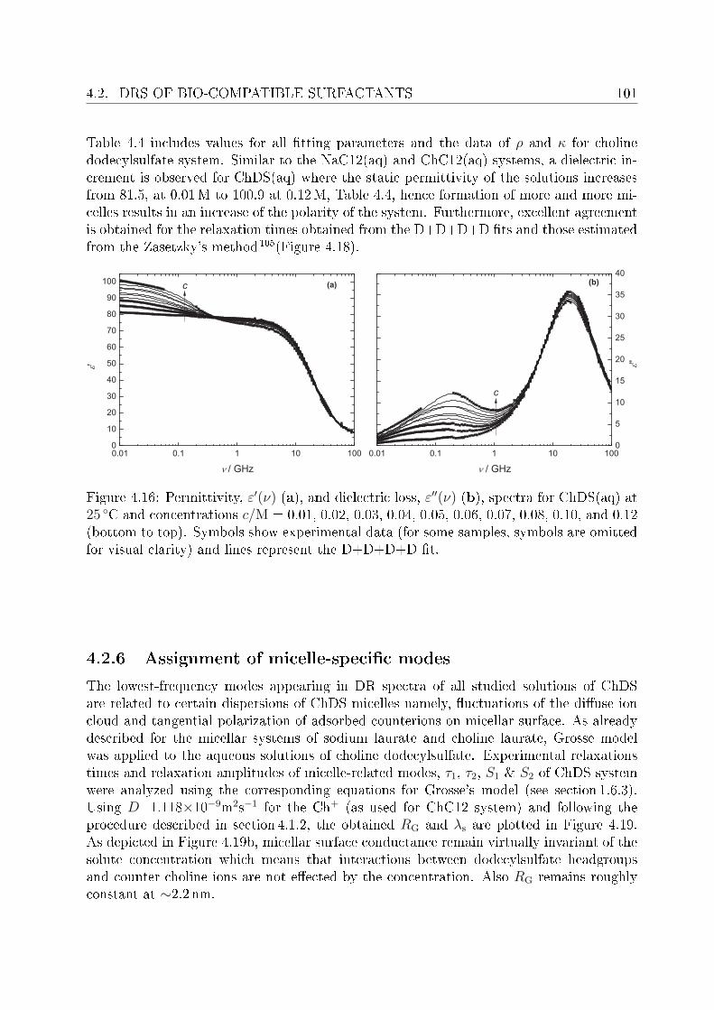
4.2. DRS OF BIO-COMPATIBLE SURFACTANTS 101
Table 4.4 includes values for all tting parameters and the data of ρ and κ for cholinedodecylsulfate system. Similar to the NaC12(aq) and ChC12(aq) systems, a dielectric in-crement is observed for ChDS(aq) where the static permittivity of the solutions increasesfrom 81.5, at 0.01M to 100.9 at 0.12M, Table 4.4, hence formation of more and more mi-celles results in an increase of the polarity of the system. Furthermore, excellent agreementis obtained for the relaxation times obtained from the D+D+D+D ts and those estimatedfrom the Zasetzky's method105(Figure 4.18).
Figure 4.16: Permittivity, ε′(ν) (a), and dielectric loss, ε′′(ν) (b), spectra for ChDS(aq) at25 C and concentrations c/M = 0.01, 0.02, 0.03, 0.04, 0.05, 0.06, 0.07, 0.08, 0.10, and 0.12(bottom to top). Symbols show experimental data (for some samples, symbols are omittedfor visual clarity) and lines represent the D+D+D+D t.
4.2.6 Assignment of micelle-specic modes
The lowest-frequency modes appearing in DR spectra of all studied solutions of ChDSare related to certain dispersions of ChDS micelles namely, uctuations of the diuse ioncloud and tangential polarization of adsorbed counterions on micellar surface. As alreadydescribed for the micellar systems of sodium laurate and choline laurate, Grosse modelwas applied to the aqueous solutions of choline dodecylsulfate. Experimental relaxationstimes and relaxation amplitudes of micelle-related modes, τ1, τ2, S1 & S2 of ChDS systemwere analyzed using the corresponding equations for Grosse's model (see section 1.6.3).Using D=1.118×10⁻⁹m2s−1 for the Ch+ (as used for ChC12 system) and following theprocedure described in section 4.1.2, the obtained RG and λs are plotted in Figure 4.19.As depicted in Figure 4.19b, micellar surface conductance remain virtually invariant of thesolute concentration which means that interactions between dodecylsulfate headgroupsand counter choline ions are not eected by the concentration. Also RG remains roughlyconstant at ∼2.2 nm.
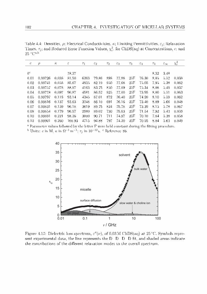
102 CHAPTER 4. INVESTIGATION OF MICELLAR SYSTEMS
Table 4.4: Densities, ρ; Electrical Conductivities, κ; Limiting Permittivities, εj; RelaxationTimes, τj; and Reduced Error Function Values, χ2
r , for ChDS(aq) at Concentrations, c; and25 Ca,b
c ρ κ ε τ1 ε2 τ2 ε3 τ3 ε4 τ4 ε∞ χ2r
0c 78.37 8.32 3.480.01 0.99726 0.038 81.50 6363 79.86 898 77.88 25F 76.30 8.05 5.52 0.0380.02 0.99741 0.058 85.67 4935 82.19 950 77.68 25F 75.05 7.95 5.38 0.0620.03 0.99757 0.078 88.97 4163 83.75 850 77.09 25F 75.34 8.08 5.49 0.0370.04 0.99778 0.097 90.87 4581 86.52 925 77.00 25F 73.95 8.00 5.51 0.0630.05 0.99797 0.118 93.14 4345 87.01 872 76.40 25F 74.20 8.10 5.59 0.0620.06 0.99816 0.137 93.63 3248 86.10 691 76.16 25F 73.40 8.09 5.66 0.0480.07 0.99831 0.159 96.18 3619 89.75 824 75.78 25F 73.39 8.15 5.78 0.0670.08 0.99854 0.179 96.57 2980 89.02 730 75.63 25F 71.54 7.92 5.43 0.0590.10 0.99891 0.221 98.36 3000 90.71 711 74.97 25F 70.10 7.84 5.38 0.0580.12 0.99921 0.260 100.93 4715 94.88 797 74.20 25F 70.25 8.04 5.63 0.049a Parameter values followed by the letter F were held constant during the tting procedure.b Units: c in M, κ in Ω−1m−1; τj in 10−12 s. c Reference 86.
Figure 4.17: Dielectric loss spectrum, ε′′(ν), of 0.03M ChDS(aq) at 25 C. Symbols repre-sent experimental data, the line represents the D+D+D+D t, and shaded areas indicatethe contributions of the dierent relaxation modes to the overall spectrum.
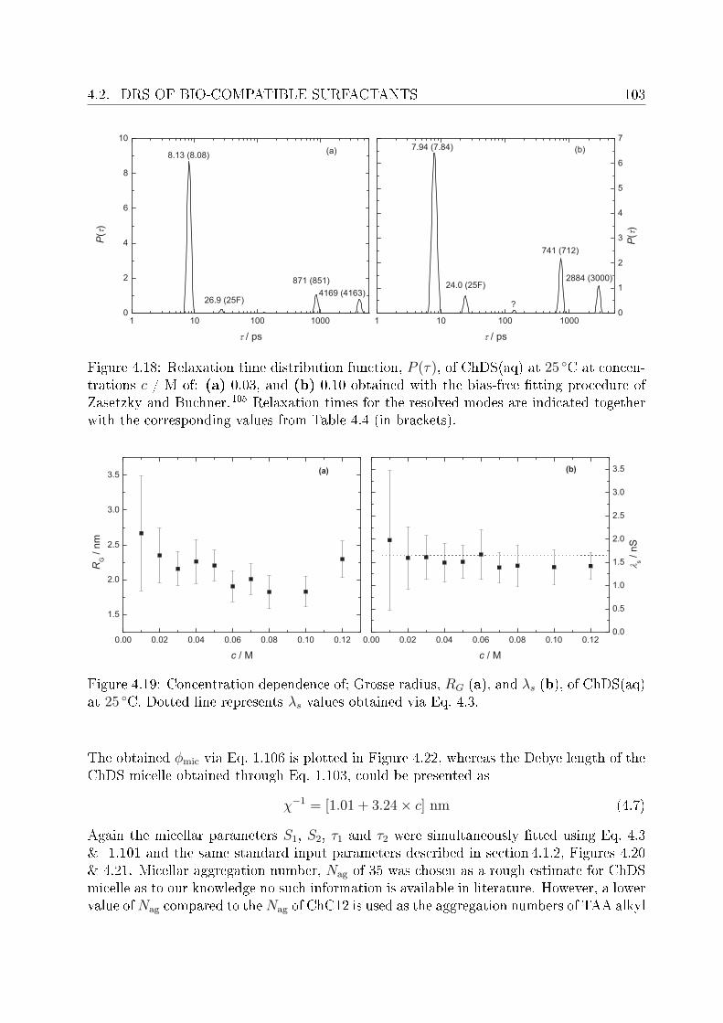
4.2. DRS OF BIO-COMPATIBLE SURFACTANTS 103
Figure 4.18: Relaxation time distribution function, P (τ), of ChDS(aq) at 25 C at concen-trations c / M of: (a) 0.03, and (b) 0.10 obtained with the bias-free tting procedure ofZasetzky and Buchner.105 Relaxation times for the resolved modes are indicated togetherwith the corresponding values from Table 4.4 (in brackets).
Figure 4.19: Concentration dependence of; Grosse radius, RG (a), and λs (b), of ChDS(aq)at 25 C. Dotted line represents λs values obtained via Eq. 4.3.
The obtained ϕmic via Eq. 1.106 is plotted in Figure 4.22, whereas the Debye length of theChDS micelle obtained through Eq. 1.103, could be presented as
χ−1 = [1.01 + 3.24× c] nm (4.7)
Again the micellar parameters S1, S2, τ1 and τ2 were simultaneously tted using Eq. 4.3& 1.101 and the same standard input parameters described in section 4.1.2, Figures 4.20& 4.21. Micellar aggregation number, Nag of 35 was chosen as a rough estimate for ChDSmicelle as to our knowledge no such information is available in literature. However, a lowervalue ofNag compared to theNag of ChC12 is used as the aggregation numbers of TAA alkyl
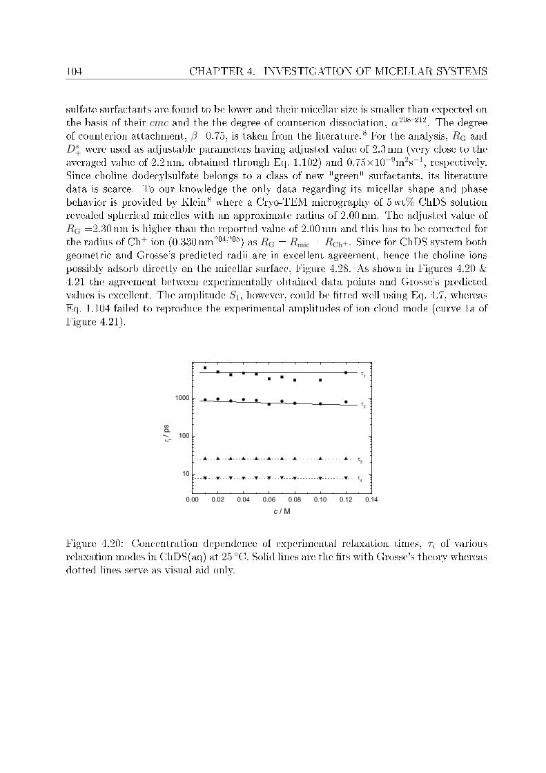
104 CHAPTER 4. INVESTIGATION OF MICELLAR SYSTEMS
sulfate surfactants are found to be lower and their micellar size is smaller than expected onthe basis of their cmc and the the degree of counterion dissociation, α208212. The degreeof counterion attachment, β=0.75, is taken from the literature.8 For the analysis, RG andDs
+ were used as adjustable parameters having adjusted value of 2.3 nm (very close to theaveraged value of 2.2 nm, obtained through Eq. 1.102) and 0.75×10⁻⁹m2s−1, respectively.Since choline dodecylsulfate belongs to a class of new "green" surfactants, its literaturedata is scarce. To our knowledge the only data regarding its micellar shape and phasebehavior is provided by Klein8 where a Cryo-TEM micrography of 5wt% ChDS solutionrevealed spherical micelles with an approximate radius of 2.00 nm. The adjusted value ofRG =2.30 nm is higher than the reported value of 2.00 nm and this has to be corrected forthe radius of Ch+ ion (0.330 nm204,205) as RG = Rmic + RCh+ . Since for ChDS system bothgeometric and Grosse's predicted radii are in excellent agreement, hence the choline ionspossibly adsorb directly on the micellar surface, Figure 4.28. As shown in Figures 4.20 &4.21 the agreement between experimentally obtained data points and Grosse's predictedvalues is excellent. The amplitude S1, however, could be tted well using Eq. 4.7, whereasEq. 1.104 failed to reproduce the experimental amplitudes of ion cloud mode (curve 1a ofFigure 4.21).
0.00 0.02 0.04 0.06 0.08 0.10 0.12 0.14
10
100
1000
4
3
2
i / ps
c / M
1
Figure 4.20: Concentration dependence of experimental relaxation times, τi of variousrelaxation modes in ChDS(aq) at 25 C. Solid lines are the ts with Grosse's theory whereasdotted lines serve as visual aid only.
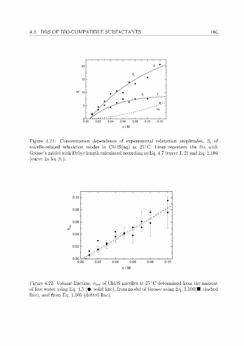
4.2. DRS OF BIO-COMPATIBLE SURFACTANTS 105
0.00 0.02 0.04 0.06 0.08 0.10 0.120
5
10
15
20
1a
1
2
S1
Si
c / M
S2
Figure 4.21: Concentration dependence of experimental relaxation amplitudes, Si ofmicelle-related relaxation modes in ChDS(aq) at 25 C. Lines represent the ts withGrosse's model with Debye length calculated according to Eq. 4.7 (curve 1, 2) and Eq. 1.104(curve 1a for S1).
0.00 0.02 0.04 0.06 0.08 0.100.00
0.02
0.04
0.06
0.08
0.10
m
ic
c / M
Figure 4.22: Volume fraction, ϕmic of ChDS micelles at 25 C determined from the amountof free water using Eq. 4.5 ( , solid line), from model of Grosse using Eq. 1.106(, dashedline), and from Eq. 1.101 (dotted line).

106 CHAPTER 4. INVESTIGATION OF MICELLAR SYSTEMS
Figure 4.22 shows ϕmic obtained from Eq. 1.106, 1.101 and 4.5. Excellent agreement isachieved between the values obtained from dierent approaches and this strongly supportsthe selection of D+D+D+D model for ChDS system. Table 4.5 includes adjusted valuesof Grosse's parameters pertaining to studied systems.
Table 4.5: Adjusted values of RG, literature values of radii, RLit, adjusted values ofDs+, and
values for the ratio, Ds+/D, for NaC12(aq), ChC12(aq), ChDS(aq) and SDS(aq) systems.
RG/ nm RLit/ nm Ds+/ m2s−1 Ds
+/ D
NaC12 2.5 2.37-2.58193 0.65×10⁻⁹ 0.49ChC12 2.7 2.1194 1.05×10⁻⁹ 0.94ChDS 2.3 2.08 0.75×10⁻⁹ 0.67SDS 2.64 (at cmc)15 2.23213 1.15×10−9,15 0.8615
Based on Collins's concept,17,18 ions are divided into two classes; kosmotropes, i.e., smallions with high charge density (hard) and chaotropes, i.e., big ions with low charge den-sity (soft). Accordingly, sodium can be considered as a "kosmotrope" and choline as"chaotrope". Interestingly, summarizing the results of presented chapter leads to a con-crete evidence that Collins's concept is obeyed by the studied micellar solutions. This canbe understood by analyzing the RG and RLit values reported in Table 4.5. It can be con-cluded that the interaction between Na+...RCO−
2 in NaC12 micelles and Ch+...ROSO−3 in
ChDS micelles is strong, hence, counterions are directly attached on the respective head-groups (see Figures 4.26 & 4.28). In case of ChC12 and SDS micelles,15 however, theinteractions between Ch+...RCO−
2 and Na+...ROSO−3 pairs is relatively weak and is water
mediated (see Figure 4.27).Furthermore, as shown in Figures 4.5b, 4.12b & 4.19b, surface conductance of the studiedmicellar systems varies with the order as λNaC12
s ∼ λChC12s > λChDS
s . Smaller size of sodiumcompared to choline ion is responsible for the larger λs of NaC12 compared to ChDS micelleswhereas weak binding of choline (compared to sodium) to the dodecanoate headgroup leadsto λNaC12
s ∼ λChC12s . Strong counterion-headgroup binding in NaC12 & ChDS (hard-hard
pairing) and weak counterion-headgroup interactions in ChC12 & SDS (soft-hard binding)micelles is also indicated by the ratio Ds
+/D (see Table 4.5) as this ratio value is highfor ChC12 compared to NaC12 micelles, similarly, Ds
+/D of SDS15 is larger than ChDSmicelle. Interestingly, all these observations conform to the Figure 4.1.
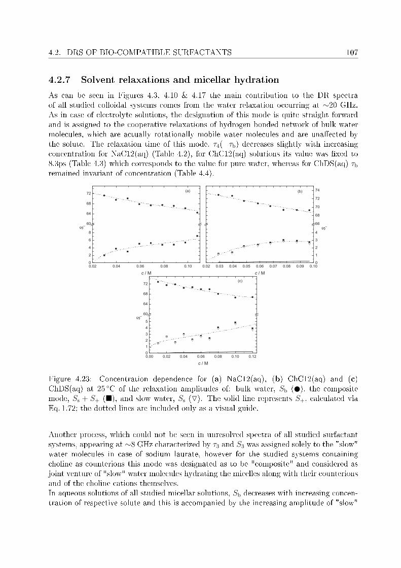
4.2. DRS OF BIO-COMPATIBLE SURFACTANTS 107
4.2.7 Solvent relaxations and micellar hydration
As can be seen in Figures 4.3, 4.10 & 4.17 the main contribution to the DR spectraof all studied colloidal systems comes from the water relaxation occurring at ∼20 GHz.As in case of electrolyte solutions, the designation of this mode is quite straight forwardand is assigned to the cooperative relaxations of hydrogen bonded network of bulk watermolecules, which are actually rotationally mobile water molecules and are unaected bythe solute. The relaxation time of this mode, τ4(=τb) decreases slightly with increasingconcentration for NaC12(aq) (Table 4.2), for ChC12(aq) solutions its value was xed to8.3ps (Table 4.3) which corresponds to the value for pure water, whereas for ChDS(aq) τbremained invariant of concentration (Table 4.4).
Figure 4.23: Concentration dependence for (a) NaC12(aq), (b) ChC12(aq) and (c)ChDS(aq) at 25 C of the relaxation amplitudes of: bulk water, Sb ( ), the compositemode, Ss + S+ (), and slow water, Ss (). The solid line represents S+, calculated viaEq. 1.72; the dotted lines are included only as a visual guide.
Another process, which could not be seen in unresolved spectra of all studied surfactantsystems, appearing at ∼8 GHz characterized by τ3 and S3 was assigned solely to the "slow"water molecules in case of sodium laurate, however for the studied systems containingcholine as counterions this mode was designated as to be "composite" and considered asjoint venture of "slow" water molecules hydrating the micelles along with their counterionsand of the choline cations themselves.In aqueous solutions of all studied micellar solutions, Sb decreases with increasing concen-tration of respective solute and this is accompanied by the increasing amplitude of "slow"

108 CHAPTER 4. INVESTIGATION OF MICELLAR SYSTEMS
water process, Ss in NaC12(aq) and "composite" mode, Sc = Ss + S+ in ChC12(aq) andChDS(aq) (Figure 4.23).Cavell equation (Eq. 1.72) was used to relate the amplitudes of various processes to theconcentration of species responsible for respective process and by using the solvent nor-malized Cavell equation, concentration of various types of water like cap,bs , cap,ss and cap,ts
was calculated by inserting the amplitudes of "bulk" water, S4, "slow" water, S3 or to-tal water amplitude, S3 + S4, respectively and the obtained values were compared to theanalytical water concentration, cs, that was obtained from the density data of solutions.For all studied surfactant systems, it was observed that at c >0, cs > cap,ts . This is inaccordance to what is already observed for some cationic surfactants (alkyltrimethylam-monium halides, CnTAX),80 however in contrast to SDS solutions where it was observedthat cap,ts = (1.002 ± 0.002) × cs.15 Hence in solutions of sodium laurate, choline laurateand choline dodecylsulfate some of the water is irrotationally bound, due to strong solute-solvent interactions and is unable to contribute to the dielectric spectrum. The quantityof such irrotationally bound or "frozen" water molecules was calculated.Since obtained Zib values through Eq. 3.12 correspond to total salt unit so in order toassign individual values to headgroups and counterions, these values should be partitionedusing the assumption of ionic additivity214. Figure 4.24 represents the Zib values per head-groups for respective micellar system. This means that the eective hydration numberof irrotationally bound water molecules is corrected for the Zib values for counterions asboth Na+,98 and Ch+,215 ions are known to freeze water molecules in there hydration shells.After correcting for Zib(Na+), a constant value of Zib ∼5 is obtained per dodecanoate head-group in sodium laurate micelle. It is interesting to note that in contrast to SDS solutionswhere no irrotational bounding was observed, Na+ ions keep their hydration in sodiumlaurate solutions. This observation receives support from the literature data provided byGustavsson and Lindman216 according to which sodium ions retain their primary hydrationwhen incorporated to alkanoate micelles. Despite the fact that Zib(-COO−, 0)=0, observedfor simple electrolyte solutions73, there is no reason to expect similar behavior of carboxy-late group in surfactant solutions where its connected to long alkyl chain. Moreover, itis not certain that obtained Zib ∼5 obtained per headgroup for sodium laurate systemcorresponds to headgroup only. Also the literature suggests existence of hydrogen bondingbetween a water molecule in the hydration shell of sodium and the carboxylate group217,thus irrotational bounding of water by NaC12 micelles could be classied as hydrophillicand at innite dilution (c→0), per NaC12 unit, 8-9 water molecules are frozen in DRS timescale.In case of choline dodecanoate, as can be seen in Figure 4.24, non-zero values of Zib
are obtained only for last three studied concentrations which range between 1-2 whereasfor all lower concentrations negative values are obtained, which is unreasonable. Thusconsidering the size of error bars Zib=0 could be assigned to per headgroup in cholinedodecanoate sytem. Whereas choline retains its hydration water (see chapter 3 for cholinehydration) with Zib(Ch+, 0)=5,215 so all the irrotational bounding observed in ChC12system corresponds solely to choline ions. The number of frozen water molecules perdodecylsulfate headgroup vary between 2-5 in ChDS micelles and similar to the ChC12system, choline as counterion retain its hydration in ChDS micelles with ve irrotationally

4.2. DRS OF BIO-COMPATIBLE SURFACTANTS 109
0.02 0.04 0.06 0.08 0.10 0.12-10
-5
0
5
10
15
20
Z ib
c / M
Figure 4.24: Concentration dependence of eective headgroup hydration numbers, Zib, at25 C for NaC12(aq) (H), ChC12(aq) ( ), and ChDS(aq) () (error bars174 are omitted forfew initial concentrations for visual clarity). Dotted lines are used only as a visual guide.
bound water molecules, whereas the whole ChDS unit, at innite dilution is able to freezeapproximately 10 water molecules.Similar to Zib, a hydration number, Zs can be dened for "slow" water molecules viaEq. 3.13. Motion of such water molecules is perturbed because of adjacent hydrophobicsurface.12 Sluggish dynamics of water molecules near the hydrophobic surface is explainedby screening eect of solute, that actually reduces the access of perturbing fth watermolecule that is required for the rearrangement of hydrogen bond network.80 Eectivenumber of slow water molecules have been calculated in the presented study for NaC12,ChC12 and ChDS micellar solutions and the values are plotted versus concentration inFigure 4.25. The presented data points however, correspond to per headgroup only asthe values are already corrected for Zib(Ch+).215 Here it should be noted that DRS stud-ies of aqueous solutions of electrolytes have revealed that Na+ does not slow down watermolecules in its hydration shell.142,218 At innite dilution, both dodecanoate and dode-cylsulfate headgroups (having choline as counterions) slow down ∼18 water molecules,whereas the number decreases with increasing concentration. This is in close agreementwith the DRS result, Zs=20, for aqueous SDS15 and higher then the values obtained forCnTAX micelles80.
The obtained Zs values for sodium laurate are rather scattered around a value of 50. Itis surprising that despite having same headgroup in choline laurate and sodium laurate,the dodecanoate could slow down more than double the number of water molecules insodium laurate compared to choline laurate. This observation on the one hand might
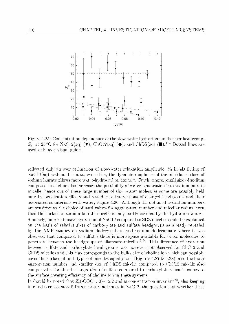
110 CHAPTER 4. INVESTIGATION OF MICELLAR SYSTEMS
0.02 0.04 0.06 0.08 0.10 0.120
10
20
30
40
50
60
70
Z s
c / M
Figure 4.25: Concentration dependence of the slow-water hydration number per headgroup,Zs, at 25 C for NaC12(aq) (H), ChC12(aq) ( ), and ChDS(aq) ().174 Dotted lines areused only as a visual guide.
reected only an over estimation of slow-water relaxation amplitude, S3 in 4D tting ofNaC12(aq) system. If not so, even then, the dynamic roughness of the micellar surface ofsodium laurate allows more water-hydrocarbon contact. Furthermore, small size of sodiumcompared to choline also increases the possibility of water penetration into sodium lauratemicelle, hence out of these large number of slow water molecules some are possibly heldonly by penetration eects and rest due to interactions of charged headgroups and theirassociated counterions with water, Figure 4.26. Although the obtained hydration numbersare sensitive to the choice of used values for aggregation number and micellar radius, eventhen the surface of sodium laurate micelle is only partly covered by the hydration water.Similarly, more extensive hydration of NaC12 compared to SDS micelles could be explainedon the basis of relative sizes of carboxylate and sulfate headgroups as already revealedby the NMR studies on sodium dodecylsulfate and sodium dodecanoate where it wasobserved that compared to sulfates there is more space available for water molecules topenetrate between the headgroups of alkanoate micelles219. This dierence of hydrationbetween sulfate and carboxylate head groups was however not observed for ChC12 andChDS micelles and this may corresponds to the bulky size of choline ion which can possiblycover the surface of both types of micelles equally well (Figures 4.27 & 4.28), also the loweraggregation number and smaller size of ChDS micelle compared to ChC12 micelle alsocompensates for the the larger size of sulfate compared to carboxylate when it comes tothe surface covering eciency of choline ion in these systems.It should be noted that Zs(-COO−, 0)∼ 5.2 and is concentration invariant73, also keepingin mind a constant ∼ 5 frozen water molecules in NaC12, the question that whether these
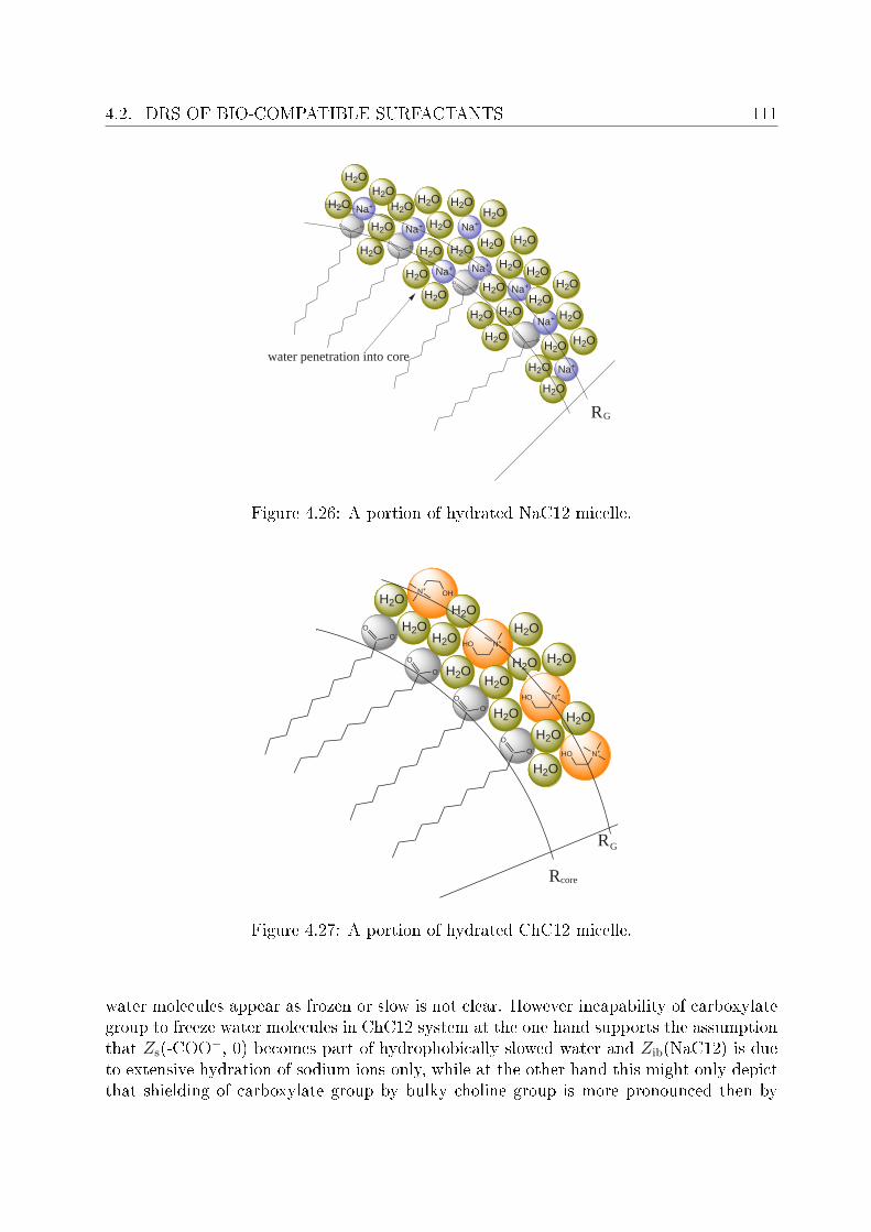
4.2. DRS OF BIO-COMPATIBLE SURFACTANTS 111
OO-
OO-
Na+
Na+
H2O
H2O
H2O
H2O
Na+
H2O
H2O
O
O-
Na+H2O H2O
H2O
Na+
H2O
H2O
H2O
H2O
Na+
Na+
H2O
H2O
H2O
H2O
O O-
Na+
H2O
H2O
H2OH2O
H2OH2O
RG
H2O
H2O
H2O
H2O
H2O
H2O
water penetration into core
Figure 4.26: A portion of hydrated NaC12 micelle.
O
O-
H2O
O
O-
HO N+
H2O
OO-
H2O
H2O
H2O
H2O
HO N+
OHN+
H2O
H2O
H2O
H2O
H2O
H2O
OO-
HO N+
H2O
Rcore
RG
Figure 4.27: A portion of hydrated ChC12 micelle.
water molecules appear as frozen or slow is not clear. However incapability of carboxylategroup to freeze water molecules in ChC12 system at the one hand supports the assumptionthat Zs(-COO−, 0) becomes part of hydrophobically slowed water and Zib(NaC12) is dueto extensive hydration of sodium ions only, while at the other hand this might only depictthat shielding of carboxylate group by bulky choline group is more pronounced then by

112 CHAPTER 4. INVESTIGATION OF MICELLAR SYSTEMS
SO
O
O
O
HO N+
H2O
SO
O
O
O
H2O
HO N+
SO
O
O
O
H2O
H2O
SO
O
O
O
HO N+
H2O
H2O
H2O
H2OHO N+
H2O
H2O
S
O
O
O
O
H2O
H2O
Rcore
RG
Figure 4.28: A portion of hydrated ChDS micelle.
small sodium ions.
4.2.8 Eect of added salt on dielectric properties of choline dode-
cylsulfate
In order to have qualitative information about the eect of added salt on the dielectricproperties of micellar systems, three dierent concentrations of each; common alkali salt,NaCl and ChCl were prepared in 0.03M ChDS(aq) solutions. Since the DR behavior andhydration of ChDS(aq) is already discussed (section 4.2.4), so stress will be given only onthe changes that occur in the dielectric spectra of 0.03M ChDS(aq) solutions containingthe added electrolyte. The obtained spectra are displayed in Figure 4.30. As mentionedbefore (section 4.2.4) the low frequency data resulted in o sets of data points in theregion where TDR and "high temperature" probe data joins, hence, in this frequencyrange few data points had to be removed in order to avoid biasing of results in terms ofnumber of modes and values of obtained dielectric parameters. For both types of systemsi.e. solutions of NaCl and ChCl in 0.03M ChDS(aq), dierent mathematical models weretested and similar to the aqueous solutions of ChDS the spectra were best described by asuperposition of four Debye (D+D+D+D) processes, see Figure 4.31 for resolved modes andTable 4.6 for the tting parameters. This is logical as added sodium is unable to produceany separate DR signal while the relaxation of added choline ions again seems to remainsubmerged with solvent relaxation peak. Compared to the solution of 0.03M ChDS(aq), thestatic permittivities of the solutions containing NaCl and ChCl are higher which indicates
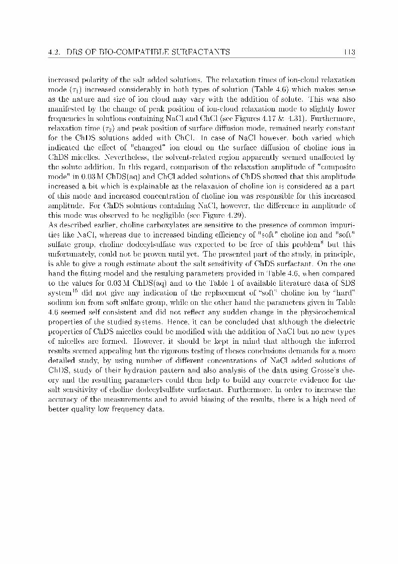
4.2. DRS OF BIO-COMPATIBLE SURFACTANTS 113
increased polarity of the salt added solutions. The relaxation times of ion-cloud relaxationmode (τ1) increased considerably in both types of solution (Table 4.6) which makes senseas the nature and size of ion cloud may vary with the addition of solute. This was alsomanifested by the change of peak position of ion-cloud relaxation mode to slightly lowerfrequencies in solutions containing NaCl and ChCl (see Figures 4.17 & 4.31). Furthermore,relaxation time (τ2) and peak position of surface diusion mode, remained nearly constantfor the ChDS solutions added with ChCl. In case of NaCl however, both varied whichindicated the eect of "changed" ion cloud on the surface diusion of choline ions inChDS micelles. Nevertheless, the solvent-related region apparently seemed unaected bythe solute addition. In this regard, comparison of the relaxation amplitude of "compositemode" in 0.03M ChDS(aq) and ChCl added solutions of ChDS showed that this amplitudeincreased a bit which is explainable as the relaxation of choline ion is considered as a partof this mode and increased concentration of choline ion was responsible for this increasedamplitude. For ChDS solutions containing NaCl, however, the dierence in amplitude ofthis mode was observed to be negligible (see Figure 4.29).As described earlier, choline carboxylates are sensitive to the presence of common impuri-ties like NaCl, whereas due to increased binding eciency of "soft" choline ion and "soft"sulfate group, choline dodecylsulfate was expected to be free of this problem8 but thisunfortunately, could not be proven until yet. The presented part of the study, in principle,is able to give a rough estimate about the salt sensitivity of ChDS surfactant. On the onehand the tting model and the resulting parameters provided in Table 4.6, when comparedto the values for 0.03M ChDS(aq) and to the Table 1 of available literature data of SDSsystem15 did not give any indication of the replacement of soft choline ion by hardsodium ion from soft sulfate group, while on the other hand the parameters given in Table4.6 seemed self consistent and did not reect any sudden change in the physicochemicalproperties of the studied systems. Hence, it can be concluded that although the dielectricproperties of ChDS micelles could be modied with the addition of NaCl but no new typesof micelles are formed. However, it should be kept in mind that although the inferredresults seemed appealing but the rigorous testing of theses conclusions demands for a moredetailed study, by using number of dierent concentrations of NaCl added solutions ofChDS, study of their hydration pattern and also analysis of the data using Grosse's the-ory and the resulting parameters could then help to build any concrete evidence for thesalt sensitivity of choline dodecylsulfate surfactant. Furthermore, in order to increase theaccuracy of the measurements and to avoid biasing of the results, there is a high need ofbetter quality low-frequency data.
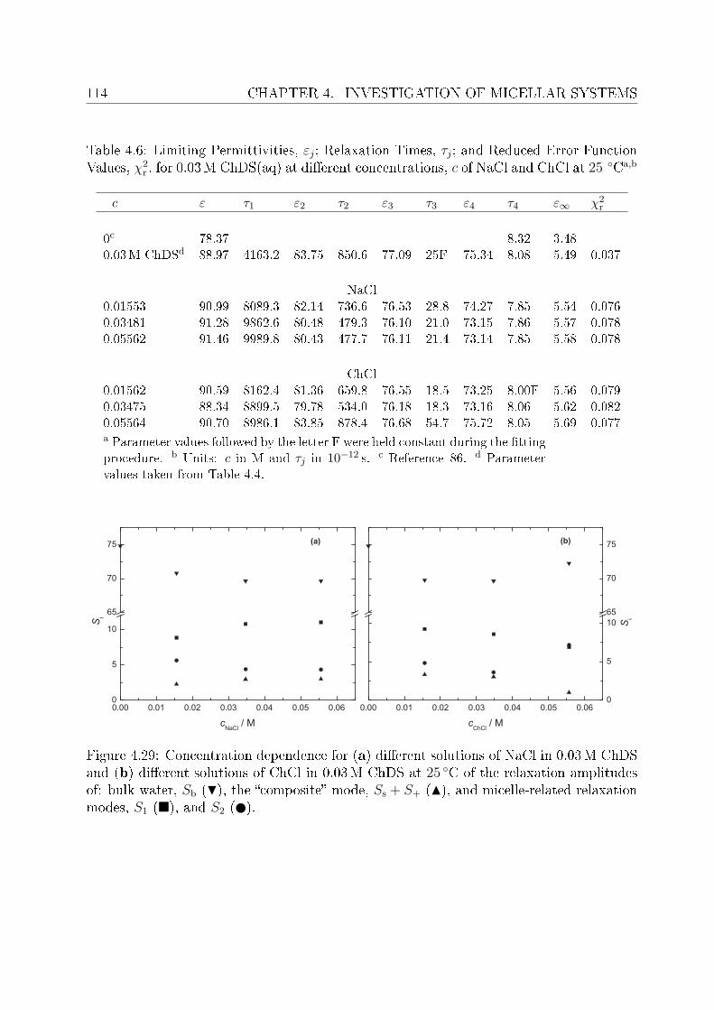
114 CHAPTER 4. INVESTIGATION OF MICELLAR SYSTEMS
Table 4.6: Limiting Permittivities, εj; Relaxation Times, τj; and Reduced Error FunctionValues, χ2
r , for 0.03M ChDS(aq) at dierent concentrations, c of NaCl and ChCl at 25 Ca,b
c ε τ1 ε2 τ2 ε3 τ3 ε4 τ4 ε∞ χ2r
0c 78.37 8.32 3.480.03M ChDSd 88.97 4163.2 83.75 850.6 77.09 25F 75.34 8.08 5.49 0.037
NaCl0.01553 90.99 8089.3 82.14 736.6 76.53 28.8 74.27 7.85 5.54 0.0760.03481 91.28 9862.6 80.48 479.3 76.10 21.0 73.15 7.86 5.57 0.0780.05562 91.46 9989.8 80.43 477.7 76.11 21.4 73.14 7.85 5.58 0.078
ChCl0.01562 90.59 8162.4 81.36 659.8 76.55 18.5 73.25 8.00F 5.56 0.0790.03475 88.34 8899.5 79.78 534.0 76.18 18.3 73.16 8.06 5.62 0.0820.05564 90.70 8986.1 83.85 878.4 76.68 54.7 75.72 8.05 5.69 0.077a Parameter values followed by the letter F were held constant during the ttingprocedure. b Units: c in M and τj in 10−12 s. c Reference 86. d Parametervalues taken from Table 4.4.
Figure 4.29: Concentration dependence for (a) dierent solutions of NaCl in 0.03M ChDSand (b) dierent solutions of ChCl in 0.03M ChDS at 25 C of the relaxation amplitudesof: bulk water, Sb (H), the composite mode, Ss + S+ (N), and micelle-related relaxationmodes, S1 (), and S2 ( ).
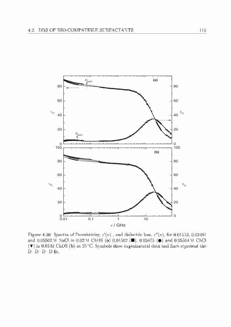
4.2. DRS OF BIO-COMPATIBLE SURFACTANTS 115
Figure 4.30: Spectra of Permittivity, ε′(ν) , and dielectric loss, ε′′(ν), for 0.01553, 0.03481and 0.05562M NaCl in 0.03M ChDS (a) 0.01562 (), 0.03475 ( ) and 0.05564M ChCl(H) in 0.03M ChDS (b) at 25 C. Symbols show experimental data and lines represent theD+D+D+D t.
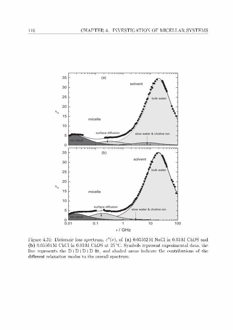
116 CHAPTER 4. INVESTIGATION OF MICELLAR SYSTEMS
Figure 4.31: Dielectric loss spectrum, ε′′(ν), of (a) 0.05562M NaCl in 0.03M ChDS and(b) 0.05564M ChCl in 0.03M ChDS at 25 C. Symbols represent experimental data, theline represents the D+D+D+D t, and shaded areas indicate the contributions of thedierent relaxation modes to the overall spectrum.

Summary and conclusions
The present thesis includes systematic broadband DRS study of choline-containing elec-trolytes and surfactants. Supplementary data for the physical properties of these systemsis also provided. For electrolyte solutions special emphasis is given to the study of ionpairing and ion hydration whereas micellar solutions are characterized on the basis of theirhydration behavior and headgroup-counterion binding. In this regard carboxylate (CO−
2 )and sulfate (OSO−
3 ) as headgroups, while Na+ and Ch+ as counterions were chosen. More-
over, salt sensitivity of choline dodecylsulfate was also studied qualitatively. In additionto the choline-based systems, aqueous solutions of NH4Cl(aq) and sodium dodecanoate(NaC12(aq)) were chosen as reference systems for the comparison purpose, hence, werestudied in detail.
Choline-based electrolytes
Electrical conductivities (at 25 C) and densities (in the range, 0-45 C) of aqueous solu-tions of choline chloride (ChCl), chlorocholine chloride (Cl-ChCl) and NH4Cl are reported.The dynamic viscosities (in the range, 0-45 C) are also provided for ChCl(aq) and Cl-ChCl(aq). The obtained data were compared with the available literature values for thestudied systems. Conductivities are well tted by the Casteel-Amis equation, Eq. 3.1,whereas low-order polynomials (Eq. 3.2) were used to t ρ(m) and η(m). Apparent molarvolumes calculated from ρ (only for ChCl(aq) and Cl-ChCl(aq)) are well described by theRedlich-Meyer approach, Eq. 3.4. The obtained sensitivity parameter, h, suggest at bestweak ion pairing for ChCl(aq) and Cl-ChCl(aq), whereas the Walden product at 25 Cpoints at signicant ion-ion interactions and/or changes in ion hydration with rising con-centration. The small but notable dierence in the h values of ChCl(aq) and Cl-ChCl(aq),as well as the dierent concentration dependence of the activation energy of viscous owmight indicate that solvation eects predominate.DRS data of all the studied electrolyte solutions did exhibit a small amplitude low fre-quency process (occurring at <1GHz), which is fairly assigned to the ion-pairs and/orion-cloud relaxation in each of these electrolyte solutions. Ion-pair association constantsare determined for the studied systems assuming that this lowest frequency process is solelydue to presence of ion-pairs in these systems, reasonable values are obtained for each ofthe studied systems which in practise could serve only as an upper limit for the possibleassociation in the studied systems.Two types of hydration are observed in aqueous solutions of ChCl and Cl-ChCl as thenumbers obtained for strongly bound, Zib, and moderately bound water molecules, Zs, are
117
118 SUMMARY AND CONCLUSIONS
non-zero for them. However, for aqueous solutions of NH4Cl no irrotational bounding ofwater molecules has been observed. For all three studied electrolyte systems Zs decreasesstrongly with increasing concentration of respective salt which indicates presence of labilehydration spheres, which is consistent with the Walden product results of ChCl and Cl-ChCl at 25 C. Also the relaxation time of bulk water mode, τb remains fairly constantfor ChCl(aq) and decreases for Cl-ChCl(aq) and NH4Cl(aq) which shows that bulk waterdynamics is not aected by the ChCl(aq) while Cl-Ch+ and NH+
4 ions aect the watermolecules beyond their primary hydration shells.
Choline-based surfactants
The DR spectra of post-micellar concentrations of sodium dodecanoate (NaC12(aq)),choline dodecanoate (ChC12(aq)) and choline dodecylsulfate (ChDS(aq)) over the fre-quency range 0.01 . ν/GHz ≤ 89 were recorded. Two types of micelle-related modescould be resolved for each of the studied surfactant systems. The lowest-frequency modewas assigned to the radial charge uctuations of the diuse ion cloud whereas next tothis appeared a relaxation, due to interfacial polarization of adsorbed counterions at themicellar surface. The dielectric properties of the studied colloidal systems were modeledwith the theory of Grosse and micelle-related parameters such as the radius (RG), surfaceconductance (λs), volume fraction (ϕmic) and Debye length (χ−1) were obtained throughthat analysis.Physico-chemical parameters obtained for all studied surfactant solutions were comparedwith the available literature data. Based on the dierence between RG and RLit values,it was observed that headgroup-counterion binding is strong between Na+...CO−
2 andCh+...OSO−
3 in NaC12(aq) and ChDS(aq) micelles, respectively. However, the bindingis weak for Ch+...CO−
2 and Na+...OSO−3 pairs in ChC12(aq) and SDS(aq) micelles, re-
spectively and is water mediated. This observation lead to the conclusion that for thepresented surfactants, Collins's law is obeyed.Hydration studies of the presented micellar solutions did reveal that in ChC12(aq) systemno irrotational bounding is observed for the carboxylate headgroup, whereas in NaC12(aq)and ChDS(aq) micelles, per headgroup, Zib ∼5 and ∼2-5 are obtained, respectively. Alsoit was observed that choline retains its individual hydration water, Zib(Ch+, 0)=5, inChC12(aq) and ChDS(aq) systems. After correcting for Zs(Ch+, 0)=18, the eective slow-water hydration number per headgroup were found to be ∼18 for both ChC12(aq) andChDS(aq) systems, this number decreases sharply with rising concentration of respectivesolute. The obtained Zs values for sodium laurate were rather scattered around a value of50. This might be, at the one hand, due to an over estimation of slow-water relaxationamplitude in 4D tting of NaC12(aq) system. On the other hand the `literature indi-cated' extensive hydration and surface roughness of sodium in NaC12(aq) micelle as wellas the smaller size of Na+ compared to Ch+ ion was used to argue for more hydration inNaC12(aq) micelles compared to choline-containing micelles.A rough estimate of salt sensitivity of ChDS was established by qualitatively analyzing thespectra of 0.03M ChDS(aq) with added NaCl and ChCl. The comparison of obtained DRdata with DR parameters of 0.03M ChDS(aq) and SDS(aq) did not give a clear hint for

SUMMARY AND CONCLUSIONS 119
the replacement of soft choline ion by hard sodium ion from soft sulfate group, whichconforms to the Collins's concept. However, the dielectric properties of ChDS(aq) micelleswere found to be modied with the addition of NaCl or ChCl. As a future prospect,better quality low-frequency data, which requires improved instrumentation, as well assystematically detailed DRS studies are needed to get more rigorous results of this issue.

Bibliography
[1] Lum, K.; Chandler, D.; Weeks, J. D. J. Phys. Chem. B 1999, 103, 4570.
[2] Food and Nutrition Board, Institute of Medicine, Dietary Reference Intakes for Thi-amin, Riboavin, Niacin, Vitamin B6, Folate, Vitamin B12, Pantothenic Acid, Bi-otin, and Choline, National Academic Press, Washington DC, 1998.
[3] Howe, J. C.; Williams, J. R.; Holden, J. M. USDA Database for the Choline Con-tent of Common Foods; National Academic Press: http://www.nal.usda.gov/fnic/foodcomp/Data/Choline/Choline.html, 2004.
[4] Zeisel, S. H.; Blusztajn, J. K. Ann. Rev. Nutr. 1994, 14, 269.
[5] Lindman, B. Handbook of Applied Surface and Colloid Chemistry ; ed. Holmberg, K.;John Wiley & Sons Ltd: Chichester, 2002.
[6] Schmalsteig, A.; Wasov, G. W. Handbook of Applied Surface and Colloid Chemistry ;ed. Holmberg, K.; John Wiley & Sons Ltd: England, 2002; Vol. 1.
[7] Kunz, W.; Kellermeier, R.; Klein, R.; Maurer, E.; Tourad, D. Biologically Accept-able Choline Compounds and their Use as Tensides, EP 2010-152626 (University ofRegensburg, Germany), 2010.
[8] Klein, R. Ph.D. Thesis, Regensburg, 2011.
[9] Abbott, A. P.; Barron, J. C.; Ryder, K. S.; Wilson, D. Chem. Eur. J. 2007, 13, 6495.
[10] Buchner, R.; Hefter, G. Phys. Chem. Chem. Phys. 2009, 11, 8954.
[11] Buchner, R. Pure Appl. Chem. 2008, 80, 1239.
[12] Buchner, R.; Hölzl, C.; Stauber, J.; Barthel, J. Phys. Chem. Chem. Phys. 2002, 4,2169.
[13] Mcbain, J. W.; Lee, W. W. Oil Soap 1943, 20, 17.
[14] Klein, R.; Tourad, D.; Kunz, W. Green Chem. 2008, 10, 433.
[15] Fernandez, P.; Schrödle, S.; Buchner, R.; Kunz, W. Chem. Phys. Chem. 2003, 4,1065.
121

122 BIBLIOGRAPHY
[16] Hofmeister, F. Arch. Exp. Path. Pharm. 1887, 24, 247.
[17] Collins, K. D.; Neilson, G. W.; Enderby, J. E. Biophys. Chem. 2007, 128, 95.
[18] Collins, K. D. Biophys. Chem. 2006, 119, 271.
[19] Maxwell, J. C. A Treatise on Electricity and Magnetism; Claredon Press: Oxford,1881.
[20] Greschner, G. S. Maxwellgleichungen; Hüthig: Basel, 1981.
[21] Böttcher, C. F. J.; Bordewijk, P. Theory of Electric Polarization; Elsevier: Amster-dam, 1978; Vol. 1 and 2.
[22] Falkenhagen, H. Theorie der Elektrolyte; Hirzel: Leipzig, 1971.
[23] Kremer, F.; Schönhals, A. Broadband Dielectric Spectroscopy ; Springer-Verlag: Ger-many, 2003.
[24] Barthel, J.; Buchner, R. Chem. Soc. Rev. 1992, 21, 263.
[25] Barthel, J.; Buchner, R.; Steger, H. Wiss. Zeitschr. THLM 1989, 31, 409.
[26] Cole, R. H. Ann. Rev. Phys. Chem. 1977, 28, 283.
[27] Debye, P. Polar Molecules ; Dover Publ.: New York, 1930.
[28] Pellat, H. Ann. Chim. Phys. 1899, 18, 150.
[29] Cole, K. S.; Cole, R. H. J. Chem. Phys. 1941, 9, 341.
[30] Cole, K. S.; Cole, R. H. J. Chem. Phys. 1942, 10, 98.
[31] Davidson, D. W.; Cole, R. H. J. Chem. Phys. 1950, 18, 1417.
[32] Davidson, D. W.; Cole, R. H. J. Chem. Phys. 1951, 19, 1484.
[33] Havriliak, S.; Negami, S. J. Polym. Sci., Part C 1966, 14, 99.
[34] Chalmers, J. M.; Griths, P. R. Handbook of Vibrational Spectroscopy ; WileyVCH:Weinheim, 2001.
[35] Onsager, L. J. Am. Chem. Soc. 1936, 58, 1486.
[36] Kirkwood, J. G. J. Chem. Phys. 1939, 7, 911.
[37] Fröhlich, H. Theory of Dielectrics, 2nd ed.; Oxford University Press: Oxford, 1965.
[38] Cavell, E. A. S.; Knight, P. C.; Sheikh, M. A. Trans. Faraday Soc. 1971, 67, 2225.
[39] Scholte, T. G. Physica 1949, 15, 437.

BIBLIOGRAPHY 123
[40] Barthel, J.; Hetzenauer, H.; Buchner, R. Ber. BunsenGes. Phys. Chem. 1992, 96,1424.
[41] Powles, J. G. J. Chem. Phys. 1953, 21, 633.
[42] Glarum, S. H. J. Chem. Phys. 1960, 33, 639.
[43] Madden, P.; Kivelson, D. Adv. Chem. Phys. 1984, 56, 467.
[44] Kivelson, D.; Madden, P. Annu. Rev. Phys. Chem. 1980, 31, 523.
[45] Dote, J. C.; Kivelson, D.; Schwartz, R. N. J. Phys. Chem. 1981, 85, 2169.
[46] Perrin, F. J. Phys. Radium 1934, 5, 497.
[47] Dote, J. C.; Kivelson, D. J. Phys. Chem. 1983, 87, 3889.
[48] Barthel, J.; Kleebauer, M.; Buchner, R. J. Solution Chem. 1995, 24, 1.
[49] Buchner, R.; Chen, T.; Hefter, G. J. Phys. Chem. B 2004, 108, 2365.
[50] Winkler, K.; Lindner, J.; Börsing, H.; Vöhringer, P. J. Chem. Phys. 2000, 113, 4674.
[51] Eisenberg, D.; Kauzmann, W. The structure and Properties of Water ; Clarendon:London, 1969.
[52] Rossky, P. J.; Karplus, M. J. Am. Chem. Soc. 1979, 101, 1913.
[53] Woutersen, S.; Emmerichs, U.; Bakker, H. J. Science 1997, 278, 658.
[54] Abragam, A. The Principles of Nuclear Magnetism; Clarendon: Oxford, UK, 1961.
[55] Teixeira, J.; Bellissent-Funel, M. C.; Chen, S. H.; Dianoux, A. J. Phys. Rev. A 1985,31, 1913.
[56] Barthel, J.; Bachhuber, K.; Buchner, R.; Hetzenauer, H. Chem. Phys. Lett. 1990,165, 369.
[57] Lawrence, C. P.; Skinner, J. L. J. Chem. Phys. 2003, 118, 264.
[58] Silvestrelli, P. L. J. Phys. Chem. B 2009, 113, 10728.
[59] Laage, D.; Stirnemann, G.; Sterpone, F.; Rey, J. T., R. Hynes Annu. Rev. Phys.Chem. 2011, 62, 395.
[60] Ivanov, E. N. Soviet Phys. JETP 1964, 18, 1041.
[61] Laage, D.; Hynes, J. T. J. Phys. Chem. B 2008, 112, 14230.
[62] Moore, W. J.; Hummel, D. O. Physikalische Chemie; de Gruyter: Berlin, 1986.

124 BIBLIOGRAPHY
[63] Glasstone, S.; Laidler, K. J.; Eyring, H. The Theory of Rate Processes ; McGraw Hill:New York, 1977.
[64] Buchner, R.; Barthel, J.; Stauber, J. Chem. Phys. Lett. 1999, 306, 57.
[65] Marcus, Y.; Hefter, G. Chem. Rev. 2006, 106, 4585.
[66] Buchner, R.; Samani, F.; May, P. M.; Sturm, P.; Hefter, G. Chem. Phys. Chem.2003, 4, 373.
[67] Eigen, M.; Tamm, K. Z. Electrochem. 1962, 66, 93 & 107.
[68] Hefter, G. Pure Appl. Chem. 2006, 98, 1571.
[69] Rudolph, W. W.; Irmer, G.; Hefter, G. T. Phys. Chem. Chem. Phys. 2003, 5, 5253.
[70] Robinson, R. A.; Stokes, R. H. Electrolyte Solutions, 2nd ed.; Butterworths: London,1970.
[71] Debye, P.; Falkenhagen, H. Phys. Z. 1928, 29, 121.
[72] Koryta, J.; Dvo°ák, J.; Kavan, L. Principles of Electrochemistry, 2nd ed.; John WileySons: Chichester, 1993.
[73] Rahman, H. M. A.; Hefter, G.; Buchner, R. J. Phys. Chem. B 2012, 116, 314.
[74] Fedotova, M. V.; Kruchinin, S. E.; Rahman, H. M. A.; Buchner, R. J. Mol. Liq.2011, 159, 9.
[75] Wachter, W.; Fernandez, S.; Buchner, R.; Hefter, G. J. Phys. Chem. B 2007, 111,9010.
[76] Yamaguchi, T.; Matsuoka, T.; Koda, S. J. Chem. Phys. 2009, 130, 094506.
[77] Yamaguchi, T.; Matsuoka, T.; Koda, S. J. Chem. Phys. 2007, 127, 234501.
[78] Eiberweiser, A.; Buchner, R. J. Mol. Liq. 2012, doi:10.1016/j.molliq.2012.03.025.
[79] Grosse, C. J. Phys. Chem. 1988, 92, 3905.
[80] Buchner, R.; Baar, C.; Fernandez, P.; Schrödle, S.; Kunz, W. J. Mol. Liq. 2005, 118,179.
[81] Göttmann, O.; Kaatze, U.; Petong, P. Meas. Sci. Technol. 1996, 7, 525.
[82] Buchner, R.; Barthel, J. Ber. BunsenGes. Phys. Chem. 1997, 101, 1509.
[83] Cole, R. H. J. Phys. Chem. 1975, 79, 1469.
[84] Cole, R. H.; Mashimo, S.; Winsor, P. J. Phys. Chem. 1980, 84, 786.
BIBLIOGRAPHY 125
[85] Hölzl, C. Ph.D. Thesis, Regensburg, 1998.
[86] Schrödle, S. Ph.D. Thesis, Regensburg, 2005.
[87] Barthel, J.; Buchner, R.; Eberspächer, P. N.; Münsterer, J., M. nad Stauber;Wurm, B. J. Mol. Liq. 1998, 78, 83.
[88] Grant, E. H.; Sheppard, R. J.; South, G. P. Dielectric Behaviour of BiologicalMolecules in Solution; Oxford University Press: Oxford, 1978.
[89] Kaatze, U.; Giese, K. J. Phys. E: Sci. Instrum. 1980, 13, 133.
[90] Birch, J. R.; O'Neil, G. P.; Yarwood, J.; Bennouna, M. J. Phys. E: Sci. Instrum.1982, 15, 684.
[91] Wan Abdullah, A. K.; Parker, T. J. Infrared. Phys. 1989, 29, 799.
[92] Barthel, J.; Bachhuber, K.; Buchner, R.; Hetzenauer, H.; Kleebauer, M. Ber. Bun-senGes. Phys. Chem. 1991, 95, 853.
[93] Hunger, J. Ph.D. Thesis, Regensburg, 2010.
[94] Levine, H.; Papas, C. H. J. Appl. Phys. 1951, 22, 29.
[95] Blackham, D. V.; Pollard, R. D. IEEE Trans. Instr. Meas. 1997, 46, 1093.
[96] Wölbl, J. Ph.D. Thesis, Regensburg, 1982.
[97] Schrödle, S.; Hefter, G.; Kunz, W.; Buchner, R. Langmuir 2006, 22, 924.
[98] Buchner, R.; Hefter, G.; May, P. M. J. Phys. Chem. A 1999, 103, 1.
[99] Feldman, Y.; Polygalov, E.; Ermolina, I.; Polevaya, Y.; Tsentsiper, B. Meas. Sci.Technol. 2001, 12, 1355.
[100] Bordi, F.; Cametti, C.; Gili, T. Bioelectrochemistry 2001, 54, 53.
[101] Hunger, J.; Stoppa, A.; Hefter, G.; Buchner, R. J. Phys. Chem. B 2008, 112, 12913.
[102] Gregory, A. P.; Clarke, R. N. Meas. Sci. Technol. 2007, 18, 1372.
[103] Bevington, P. R. Data Reduction and Error Analysis for the Physical Sciencies ;McGrawHill: New York, 1969.
[104] Steger, H. Ph.D. Thesis, Regensburg, 1988.
[105] Zasetsky, A. Y.; Buchner, R. J. Phys.: Condens. Matter 2011, 23, 025903.
[106] Tikhonov, A. Dokl. Acad. Nauk SSSR 1963, 151, 501.
[107] Kratky, O.; Leopold, H.; Stabinger, H. Z. Angew. Phys. 1969, 27, 273.
126 BIBLIOGRAPHY
[108] Lide, D. R., Ed. CRC Handbook of Chemistry and Physics, 85th ed.; CRC Press:Boca Raton, USA, 2004.
[109] Barthel, J.; Wachter, R.; Gores, H. J. In Modern Aspects of Electrochemistry ; Con-way, B. E., Bockris, J. O., Eds.; Plenum: New York, 1979; Vol. 13; pp 179.
[110] Barthel, J.; Graml, H.; Neueder, R.; Turq, P.; Bernard, O. Curr. Top. Solution Chem.1994, 1, 223.
[111] Stoppa, A.; Hunger, J.; Buchner, R. J. Chem. Eng. Data 2009, 54, 472.
[112] Barthel, J.; Feuerlein, F.; Neueder, R.; Wachter, R. J. Solution Chem. 1980, 9, 209.
[113] Hoover, T. B. J. Phys. Chem. 1964, 68, 876.
[114] Shaukat, S.; Buchner, R. J. Chem. Eng. Data 2011, 56, 4944.
[115] Stewart, J. J. P. MOPAC2009, Stewart Computational Chemistry, Colorado Springs,CO, USA.
[116] Stewart, J. J. P. J. Mol. Modeling 2007, 13, 1173.
[117] Baker, J. J. Com. Chem. 1986, 7, 385.
[118] Bondi, A. J. Phys. Chem. 1964, 68, 441.
[119] Senda, N. Winmostar, version 3.78f. http://winmostar.com.
[120] Marcus, Y., Ed. Ion Solvation; Wiley: Chichester, UK, 1985.
[121] Bockris, J. O.; Reddy, A. K. N. Modern Electrochemistry ; 2nd ed., Plenum: NewYork, 1998; Vol. 1.
[122] Smith, W. H. Chem. Eng. News 1991, 69, 31.
[123] Perrin, C. L.; Gipe, R. K. J. Am. Chem. Soc. 1984, 96, 5631.
[124] Perrin, C. L.; Gipe, R. K. J. Am. Chem. Soc. 1986, 108, 1088.
[125] Sharygin, A. V.; Wood, R. H. J. Chem. Thermodyn. 1996, 28, 851.
[126] Rooney, S. A. Environmental Health Perspectives 1984, 55, 205.
[127] Klein, R.; Tourad, D.; Kunz, W. Green Chem. 2008, 10, 433.
[128] Klein, R.; Kellermeier, M.; Drechsler, M.; Tourad, D.; Kunz, W. Colloids and surfacesA: Physicochem. Eng. Aspects 2009, 338, 129.
[129] Liao, J.-H.; Wu, P.-C.; Bai, Y.-H. Inorg. Chem. Commun. 2005, 8, 390.
[130] Tolbert, N. E. J. Biol. Chem. 1960, 235, 475.
BIBLIOGRAPHY 127
[131] Westhof, E. E. Water and Biological Macromolecules ; Macmillan: London, 1993.
[132] Bellissent-Funel, M.-C. E. Hydration Processes in Biology ; IOS Press: Amsterdam,1999.
[133] Billeter, M. Prog. Nucl. Mag. Res. Spectrosc. 1995, 27, 635.
[134] Wohlfarth, C. Enthalpy Data of Polymer-Solvent Systems ; CRC Press: Boca Raton,2006.
[135] Graziano, G. Can. J. Chem. 2001, 79, 1310.
[136] Wyttenbach, T.; Bowers, M. Chem. Phys. Lett. 2009, 480, 1.
[137] Buchner, R.; Barthel, J. Ann. Rep. Prog. Chem. Sect. C 2001, 97, 349.
[138] Buchner, R. Dielectric Spectroscopy of Solutions, in: J. Samios und V.A. Durov(Eds.), Novel Approaches to the Structure and Dynamics of Liquids: Experiments,Theories and Simulations, nato asi ser. ii ed.; Kluwer: Dordrecht, 2004; Vol. 133; pp. 265.
[139] Belleau, B. Ann. N. Y. Acad. Sci. 1967, 144, 705.
[140] Hefter, G.; Buchner, R. Dielectric spectroscopy: a new old tool for studying ions insolution. In : 235th National Meeting of the American Chemical Society ; AmericanChemical Society: 6 - 10 April, New Orleans, 2008.
[141] Casteel, J. F.; Amis, A. S. J. Chem. Eng. Data 1972, 17, 55.
[142] Buchner, R.; Capewell, S. G.; Hefter, G.; May, P. M. J. Phys. Chem. B 1999, 103,1185.
[143] Fleming, R. J. Chem. Soc. A 1960, 4914.
[144] Wishaw, B. F.; Stokes, R. H. J. Am. Chem. Soc. 1954, 76, 2065.
[145] McCleskey, R. B. J. Chem. Eng. Data 2011, 56, 317.
[146] Spieweck, F.; H., B. Technisches Messen 1992, 59, 285.
[147] Millero, F. J.; Hansen, W. D. J. Phys. Chem. 1968, 72, 1758.
[148] Motin, M. A. J. Chem. Eng. Data 2004, 49, 94.
[149] Pearce, J. N.; Pumplin, G. G. J. Am. Chem. Soc. 1937, 59, 1221.
[150] Albright, J. G.; Mitchell, J. P.; Miller, D. G. J. Chem. Eng. Data 1994, 39, 195.
[151] kaminsky, M. Z. Phys. Chem. N. F. 1955, 5, 154.
[152] Rashkovskaya, E. A.; Chernen'kaya, E. I. J. Appl. Chem. USSR 1967, 40, 301.
128 BIBLIOGRAPHY
[153] Desnoyers, J. E.; Arel, M. Can. J. Chem. 1967, 45, 359.
[154] Redlich, o.; Meyer, D. M. Chem. Rev. 1964, 64, 221.
[155] Millero, F. J. Chem. Rev. 1971, 71, 147.
[156] Archer, D. G.; Wang, P. J. Phys. Chem. Ref. Data 1990, 19, 371.
[157] Klofutar, C.; Horvat, J.; Rudan-Tasi£, D. Acta Chim. Slov. 2006, 53, 274.
[158] Hepler, L. G. Can. J. Chem. 1969, 47, 4613.
[159] Millero, F. J. J. Phys. Chem. 1970, 74, 356.
[160] Be²ter-Roga£, M.; Neueder, R.; Barthel, J. J. Solution Chem. 1999, 28, 1071.
[161] Wachter, W.; Buchner, R.; Hefter, G. J. Phys. Chem. B 2006, 110, 5147.
[162] Tromans, A.; May, P. M.; Hefter, G.; Sato, T.; Buchner, R. J. Phys. Chem. B 2004,108, 13789.
[163] Rønne, C.; Thrane, L.; Åstrand, P.-O.; Wallqvist, A.; Mikkelsen, K. V.; Keiding, S. R.J. Chem. Phys. 1997, 107, 5319.
[164] Morrow, T. I.; Maginn, E. Fluid Phase Equilib. 2004, 217, 97.
[165] Marlow, G. E.; Pettitt, B. Biopolymers 2003, 68, 192.
[166] Lee, H.; Wilmshurst, J. K. Aust. J. Chem. 1964, 17, 943.
[167] Impey, R. W.; Madden, P. A.; Mcdonald, I. R. J. Phys. Chem. 1993, 87, 5071.
[168] Korson., L.; Drost-Hansen., W.; Millero, F. J. J. Phys. Chem. 1969, 73, 34.
[169] Alavi, D. S.; Hartman, R. S.; Waldeck, D. H. J. Chem. Phys. 1991, 94, 4509.
[170] Hubbard, J. B.; Onsasager, L. J. Chem. Phys. 1977, 67, 4850.
[171] Hubbard, J. B. J. Chem. Phys. 1978, 68, 1649.
[172] Hubbard, J. B.; Colonomos, P.; Wolynes, P. G. J. Chem. Phys. 1979, 71, 2652.
[173] Mancinelli, R.; Botti, A.; Bruni, F.; Ricci, M. A.; Soper, A. K. Phys. Chem. Chem.Phys. 2007, 9, 2959.
[174] Error bars for Zib were calculated from the standard deviations of ts of the polyno-mial Sb(c) = Sb(0)− a1c+ a2c
3/2 with Sb(0) xed to the corresponding value of purewater taken from ref. 86, for Zs, the standard deviations were obtained via the tsof the polynomial Ss(c) = a1c+ a2c
3/2.
[175] Fleming, R. J. Chem. Soc. A 1966, 946.
BIBLIOGRAPHY 129
[176] Shao, Q.; He, Y.; White, A. D.; Jiang, S. J. Phys. Chem. B 2010, 114, 16625.
[177] Szász, G. I.; Heinzinger, K. Z. Naturforsch. 1979, 34a, 840.
[178] Bohm, H. J.; McDonald, I. R. Mol. Phys. 1984, 80, 887.
[179] Dang, L. X. Chem. Phys. Lett. 1993, 213, 541.
[180] Harmon, K.; Akin, A. C.; Avci, G. F.; Nowas, L. S. J. Mol. Struct. 1991, 244, 223.
[181] Intharathep, P.; Tongraar, A.; Sagarik, K. J. Comput. Chem. 2005, 26, 1329.
[182] Walrafen, G. E.; Fisher, M. R.; Hokmabadi, M. S.; Yang, W. H. J. Chem. Phys.1986, 85, 6970.
[183] Tanford, C. The Hydrophobic Eect-Formation of Micelles and Biological Mem-braness ; Wiley: New York, 1980.
[184] Laughlin, R. G. The Aqueous Phase Behavior of Surfactants ; Academic Press: SanDiego, 1994.
[185] Madelmont, C.; Perron, R. Colloid Polym. Sci. 1976, 254, 581.
[186] Lin, B.; McCormick, A. V.; Davis, H. T.; Strey, R. J. Colloid Interface Sci. 2005,291, 543.
[187] Preston, W. C. J. Phys. Chem. 1948, 52, 84.
[188] Shinoda, K.; Kunieda, H. J. Phys. Chem. 1976, 80, 2468.
[189] Jansson, M.; Jönsson, A.; Li, P.; Stilbs, P. Colloids Surfs. 1991, 59, 387.
[190] Zana, R. Langmuir 2004, 20, 5666.
[191] Vlachy, N.; Jagoda-Cwiklik, B.; Vácha, R.; Tourad, D.; Jungwirth, P.; Kunz, W.Adv. Colloid Interface Sci. 2009, 146, 42.
[192] Zhao, G.; Zhu, B. Princip. Surf. Action (Chin.) 2003, 242.
[193] Caponetti, E.; Martino, D. C.; Floriano, M. A.; Triolo, R. Langmuir 1993, 9, 1193.
[194] Klein, R. Diploma Thesis, Regensburg, 2006.
[195] Quina, F. H.; Nassar, P. M.; Bonilha, J. B. S.; Bales, B. L. J. Phys. Chem. 1995,99, 17028.
[196] Sasaki, T.; Hattori, M.; Sasaki, J.; Nukina, K. Bull. Chem. Soc. Jpn. 1975, 48, 1397.
[197] Baar, C.; Buchner, R.; Kunz, W. J. Phys. Chem. B 2001, 105, 2906.
[198] Pauly, H.; Schwan, H. P. Z. Naturforsch. B 1959, 14, 125.
130 BIBLIOGRAPHY
[199] R-Pulido, A.; Casado, A.; M-Úbeda, M.; Junquera, E.; Aicart, E. Langmuir 2010,26, 9378.
[200] King, D. T.; Warren, D. B.; Pouton, C. W.; Chalmers, D. K. Langmuir 2011, 27,11381.
[201] Bertolini, D.; Cassettari, M.; Salvetti, G.; Tombari, E.; Veronesi, S. Rev. Sci. In-strum. 1990, 61, 450.
[202] Hunger, J. Diploma Thesis, Regensburg, 2006.
[203] Spivey, H. O.; Snell, F. M. J. Phys. Chem. 1964, 68, 2126.
[204] Levitt, D. G.; Decker, E. R. Biophys. J. 1988, 53, 33.
[205] Abbott, A. P.; Boothby, D.; Capper, G.; Davies, D. L.; Rasheed, R. K. J. Am. Chem.Soc. 2004, 126, 9142.
[206] Gibbs, J. H.; Cohen, C.; Fleming III, P. H. i. The Physical Chemistry of AqueousSystems, ed. kay, r. l. ed.; Plenum: New York, 1973.
[207] Stache, H. W. Surfactant Science Series-Anionic Surfactants; Marcel Dekker: NewYork, 1996.
[208] Zana, R.; Benrrau, M.; Bales, B. L. J. Phys. Chem. B 2004, 108, 18195.
[209] Benrrau, M.; Bales, B. L.; Zana, R. J. Phys. Chem. B 2003, 107, 13432.
[210] Bales, B. L.; Tiguida, K.; Zana, R. J. Phys. Chem. B 2004, 108, 14948.
[211] Paul, A.; Griths, P. C.; Pettersson, E.; Stilbs, P.; Bales, B. L.; Zana, R.;Heenan, R. K. J. Phys. Chem. B 2005, 109, 15775.
[212] Tcacenco, C. M.; Zana, R.; Bales, B. L. J. Phys. Chem. B 2005, 109, 15997.
[213] Itri, R.; Amaral, L. Q. J. Phys. Chem. 1991, 95, 423.
[214] Although additivity rule is applicable only at innite dilution but due to the approx-imate nature of these calculations and consistent with previous experience,10,11,98 itis applied to nite concentrations as well.
[215] Shaukat, S. and Buchner, R. Unpublished results .
[216] Gustavsson, H.; Lindman, B. J. Am. Chem. Soc. 1978, 100, 4647.
[217] Gustavsson, H.; Lindman, B. J. Am. Chem. Soc. 1975, 97, 3923.
[218] Wachter, W.; Kunz, W.; Buchner, R.; Hefter, G. J. Phys. Chem. A 2005, 109, 8675.
[219] Halle, B.; Cariström, G. J. Phys. Chem. 1981, 85, 2142.
Regensburg, den 30.10.2012
Saadia Shaukat
131